$R^{p}$ Attractors Static Neutron Star Phenomenology

Abstract

In this work we study the neutron star phenomenology of $R^{p}$ attractor theories in the Einstein frame. The Einstein frame $R^{p}$ attractor theories have the attractor property that they originate from a large class of Jordan frame scalar theories with arbitrary non-minimal coupling. These theories in the Einstein frame provide a viable class of inflationary models, and in this work we investigate their implications on static neutron stars. We numerically solve the Tolman-Oppenheimer-Volkoff equations in the Einstein frame, for three distinct equations of state, and we provide the mass-radius diagrams for several cases of interest of the $R^{p}$ attractor theories. We confront the results with several timely constraints on the radii of specific mass neutron stars, and as we show, only a few cases corresponding to specific equations of state pass the stringent tests on neutron stars phenomenology.

Introduction

The direct gravitational wave observation GW170817 LIGO & Virgo Collaboration, et al. (2017, 2020) initiated what is nowadays known as gravitational wave astronomy. Neutron stars (NS) Haensel, Potekhin & Yakovlev (2007); (2013); Baym, et al. (2018); Lattimer & Prakash (2004); Olmo, Rubiera-Garcia & Wojnar (2020) are at the core of astrophysical gravitational wave observations, and numerous scientific areas are jointly studying NS from their perspective, for example nuclear theory Lattimer (2012); Steiner & Gandolfi (2012); Horowitz, et al. (2005); Watanabe, Iida & Sato (2000); Shen, et al. (1998); Xu, et al. (2009); Hebeler, et al. (2013); Mendoza-Temis, et al. (2014); Ho, et al. (2015); Kanakis-Pegios, Koliogiannis & Moustakidis (2020); Tsaloukidis et al. (2022), high energy physics Buschmann, et al. (2021); Safdi, Sun & Chen (2019); Hook, et al. (2018); Edwards, et al. (2020); Nurmi, Schiappacasse & Yanagida (2021), modified gravity Astashenok, et al. (2020, 2021); Capozziello, et al. (2016); Astashenok, Capozziello & Odintsov (2015, 2014, 2013); Arapoǧlu, Deliduman & Eksi (2011); Panotopoulos et al. (2021); Lobato et al. (2020); Numajiri et al. (2022) and astrophysics Altiparmak, Ecker & Rezzolla (2022); Bauswein, et al. (2020b); Vretinaris, Stergioulas & Bauswein (2020); Bauswein, et al. (2020a, 2017); Most, et al. (2018); Rezzolla, Most & Weih (2018); Nathanail, Most & Rezzolla (2021); Köppel, Bovard & Rezzolla (2019); Raaijmakers et al. (2021); Most, et al. (2021); Ecker & Rezzolla (2022); Jiang, et al. (2022). The perspective of modified gravity implications on NS has been for a long time in the mainstream of NS works, see for example Astashenok, Capozziello & Odintsov (2015, 2014) and also Refs. Pani & Berti (2003); Staykov, et al. (2014); Horbatsch, et al. (2015); Silva, et al. (2015); Doneva, et al. (2013); Xu, Gao & Shao (2020); Salgado, Sudarsky & Nucamendi (1998); Shibata, et al. (2014); Arapoğlu, Ekşi & Yükselci (2019); Ramazanoğlu & Pretorius (2016); Motahar, et al. (2019); Chew, et al. (2019); Blázquez-Salcedo, Scen Khoo & Kunz (2020); Motahar, et al. (2017); Odintsov & Oikonomou (2021, 2022a); Oikonomou (2021); Pretel et al. (2022); Pretel & Duarte (2022); Cuzinatto et al. (2016) for scalar-tensor descriptions of NS phenomenology. The main effect of modified gravity descriptions of NS is the significant elevation of the maximum NS masses, with modified gravity bringing this maximum mass near or inside the mass-gap region with $M\geq 2.5\,M_{\odot}$. Regarding non-minimally coupled scalar field theories, there exists a vast class of viable inflationary potentials which have the remarkable property of being attractors Kallosh, Linde & Roest (2014a); Kallosh & Linde (2013); Ferrara, et al. (2013); Kallosh, Linde & Roest (2013); Linde (2015); Cecotti & Kallosh (2014); Carrasco, Kallosh & Linde (2015); Carrasco, et al. (2015); Kallosh, Linde & Roest (2015); Roest & Scalisi (2015); Kallosh, Linde & Roest (2014b); Ellis, Nanopoulos & Olive (2013); Cai, Gong & Pi (2014); Yi & Gong (2016); Akrami, et al. (2018); Qummer, Jawad & Younas (2020); Fei, Yi & Yang (2020); Kanfon, Mavoa & Houndjo (2020); Antoniadis, et al. (2020); García-García, et al. (2019); Cedeño, et al. (2019); Karamitsos (2019); Canko, Gialamas & Kodaxis (2020); Miranda, et al. (2019); Karam, Pappas & Tamvakis (2019); Nozari & Rashidi (2018); García-García, et al. (2018); Rashidi & Nozari (2018); Gao, Gong & Fei (2018); Dimopoulos, Wood & Owen (2018); Miranda, Fabris & Piattella (2017); Karam, Pappas & Tamvakis (2017); Nozari & Rashidi (2017); Gao & Gong (2018); Geng, Lee & Wu (2017); Odintsov & Oikonomou (2020, 2016, 2017); Järv, et al. (2020). The attractor terminology is justified due to the fact that distinct non-minimally coupled scalar-tensor inflationary theories, lead to the same Einstein frame inflationary phenomenology, which is compatible with the latest Planck data Planck Collaboration (2020). The question always when studying these attractor models is whether these models can be distinguished in some way, phenomenologically. From an inflationary point of view, and regarding the large wavelength Cosmic Microwave Background modes, a discrimination between these models is impossible. However, this discrimination is possible if NS are studied. Indeed, the phenomenologically indistinguishable attractor models can be discriminated in NS and vice versa, with the latter feature being phenomenal. That is, if some models are indistinguishable with respect to their NS phenomenology, they can be distinguished if their inflationary properties are studied. To address these issues in a concrete way, in this work we shall study $R^{p}$ attractor theories. The inflationary phenomenology of these theories is studied in the recent literature Odintsov & Oikonomou (2022b) see also Motohashi (2015); Renzi, Shokri & Melchiorri (2009) for subcases of the original $R^{p}$ attractors theories. For a spherically symmetric metric we derive and solve numerically the Einstein frame Tolman-Oppenheimer-Volkoff (TOV) equations, using an LSODA based double shooting python 3 numerical integration Stergioulas (2019). We derive the Jordan frame $M-R$ graphs for the $R^{p}$ attractors, for three different piecewise polytropic Read, et al. (2009a, b) equations of state (EoS), WFF1 Wiringa, Fiks & Fabrocini (1988), the SLy Douchin & Haensel (2001), and the APR EoS Akmal, Pandharipande & Ravenhall (1998), using the Arnowitt-Deser-Misner (ADM) definition of Jordan frame masses of NS Arnowitt, Deser & Misner (1960). The NSs temperature is significantly lower than the Fermi energy of the constituent particles of NSs, thus NS matter can be in principle described by a single-parameter EoS that may describe perfectly cold matter at densities higher than the nuclear density. However, a serious problem emerges, having to do with the uncertainty in the EoS, which is larger, and the pressure as a function of the baryonic mass density cannot be accurately defined and is uncertain to one order of magnitude at least above the nuclear density. Moreover, the exact nature of the phase of matter at the NSs core is highly uncertain. Hence, a parameterized-type EoS at high densities is an optimal choice for an EoS, thus rendering the piecewise polytropic EoS a suitable choice. In order to construct the piecewise polytropic EoS, astrophysical constraints are taken into account, both observational and theoretical, like the causality constraints, see Read, et al. (2009a, b), to also confirm the causality fulfilment for all the piecewise polytropic EoS we shall use in this paper. For the construction of the piecewise polytropic EoS one uses a low-density part with $\rho<\rho_{0}$, which is basically chosen to be a tabulated and well-known EoS for the crust, and furthermore, the piecewise polytropic EoS also has a large density part with $\rho\gg\rho_{0}$. We finally confront the resulting NS phenomenologies with several recent constraints on the radii of specific mass NS Altiparmak, Ecker & Rezzolla (2022); Raaijmakers et al. (2021); Bauswein, et al. (2017) and as we show, only a few scenarios and EoS are compatible with the constraints on NS radii. Obviously, the gravitational wave astronomy era has changed the way of thinking on theoretical astrophysics, since several models of scalar-tensor gravity which in the recent past could be considered as viable, nowadays may no longer be valid.

1 Inflationary Phenomenology of $R^{p}$ Attractors

The full analysis of the generalized $R^{p}$ attractors is given in Ref. Odintsov & Oikonomou (2022b), so we refer the reader for details. Here we shall briefly discuss the inflationary phenomenological properties of $R^{p}$ attractors in order to stress their importance among other cosmological attractors Kallosh, Linde & Roest (2014a); Kallosh & Linde (2013); Ferrara, et al. (2013); Kallosh, Linde & Roest (2013); Linde (2015); Cecotti & Kallosh (2014); Carrasco, Kallosh & Linde (2015); Carrasco, et al. (2015); Kallosh, Linde & Roest (2015); Roest & Scalisi (2015); Kallosh, Linde & Roest (2014b); Ellis, Nanopoulos & Olive (2013); Cai, Gong & Pi (2014); Yi & Gong (2016); Akrami, et al. (2018); Qummer, Jawad & Younas (2020); Fei, Yi & Yang (2020); Kanfon, Mavoa & Houndjo (2020); Antoniadis, et al. (2020); García-García, et al. (2019); Cedeño, et al. (2019); Karamitsos (2019); Canko, Gialamas & Kodaxis (2020); Miranda, et al. (2019); Karam, Pappas & Tamvakis (2019); Nozari & Rashidi (2018); García-García, et al. (2018); Rashidi & Nozari (2018); Gao, Gong & Fei (2018); Dimopoulos, Wood & Owen (2018); Miranda, Fabris & Piattella (2017); Karam, Pappas & Tamvakis (2017); Nozari & Rashidi (2017); Gao & Gong (2018); Geng, Lee & Wu (2017); Odintsov & Oikonomou (2020, 2016, 2017); Järv, et al. (2020). The $R^{p}$ attractors constitute a class of their own among other attractors, and all the $R^{p}$ attractors in the Einstein frame correspond to generalizations of the following Einstein frame potential,

$$V(\varphi)=V_{0}\,M_{p}^{4}e^{-2\sqrt{\frac{2}{3}}\kappa\varphi}\left(e^{\sqrt{\frac{2}{3}}\kappa\varphi}-1\right)^{\frac{p}{p-1}}\,,$$ (1)

where $M_{p}=\frac{1}{\sqrt{8\pi G}}$ is the reduced Planck mass and $G$ is Newton’s gravitational constant. The inflationary properties of the above theory have been addressed in the recent literature, see for example Motohashi (2015); Renzi, Shokri & Melchiorri (2009). The scalar-tensor theory with the potential (1) corresponds to the Jordan frame $F(R)$ gravity,

$$F(R)=R+\beta R^{p}\,,$$ (2)

with $\beta$ is a free parameter with its physical dimensions in natural units being $[\beta]=[m]^{2-2p}$. The $R^{p}$ attractors have the following scalar potential in the Einstein frame,

$$V(\varphi)=V_{0}\,M_{p}^{4}e^{-2\sqrt{\frac{2}{3\alpha}}\kappa\varphi}\left(e^{\sqrt{\frac{2}{3\alpha}}\kappa\varphi}-1\right)^{\frac{p}{p-1}}\,,$$ (3)

where $M_{p}$ is the reduced Planck mass, and for $\alpha=1$ we obtain the scalar theory with scalar potential (3). Now the question is why these models are classified as attractor models, what justifies the terminology attractors? It is the class of scalar-tensor Jordan frame theories which correspond to the Einstein frame potential (3) that justify the use of the terminology attractors. Basically, the potential (3) can be the Einstein frame potential for a large class of Jordan frame scalar-tensor theories, as we now evince. The $\phi$-Jordan frame action is,

$$\mathcal{S}_{J}=\int d^{4}x\left(\frac{\Omega(\phi)}{2\kappa^{2}}R-\frac{\omega(\phi)}{2}g^{\mu\nu}\partial_{\mu}\phi\partial_{\nu}\phi-V_{J}(\phi)\right)\,,$$ (4)

with the scalar field describing a non-canonical scalar field in the Jordan frame, and the coupling function has the general form $\Omega(\phi)=1+\xi f(\phi)$ with $\xi$ and $f(\phi)$ being the arbitrary dimensionless coupling and an arbitrary dimensionless function respectively. The $R^{p}$ attractors have the following $\phi$-Jordan frame scalar potential,

$$V_{J}(\phi)=V_{0}\left(\Omega(\phi)-1\right)^{\frac{p}{p-1}}\,,$$ (5)

and more importantly, the kinetic term function $\omega(\phi)$ has the following form,

$$\omega(\phi)=\frac{1}{4\xi}\frac{\left(\frac{d\Omega(\phi)}{d\phi}\right)^{2}}{\Omega(\phi)}\,.$$ (6)

Hence the large class of the $R^{p}$-attractors correspond to the Jordan frame theories which are described by Eqs. (5) and (6). Notice that the Jordan frame functions $f(\phi)$ are arbitrary and we shall not need to specify these. By performing the conformal transformation of the Jordan frame metric $g_{\mu\nu}$,

$$\tilde{g}_{\mu\nu}=\Omega(\phi)g_{\mu\nu}\,,$$ (7)

we get the Einstein frame action,

$$\mathcal{S}_{E}=\sqrt{-\tilde{g}}\left(\frac{\tilde{R}}{2\kappa^{2}}-\tilde{g}^{\mu\nu}\partial_{\mu}\varphi\partial_{\nu}\varphi-V(\varphi)\right)\,,$$ (8)

with $\tilde{g}_{\mu\nu}$ denoting the Einstein frame metric tensor, and the “tilde” indicates Einstein frame quantities. Also the Einstein frame potential $V(\phi)$ and the Jordan frame potential $V_{J}(\phi)$ are related as follows,

$$V(\varphi)=\Omega^{-2}(\phi)V_{J}(\phi)\,.$$ (9)

Notice that the general relation which connects the Jordan frame scalar field $\phi$ with the canonical Einstein frame scalar field $\varphi$ is,

$$\left(\frac{d\varphi}{d\phi}\right)^{2}=\frac{3}{2}\frac{\left(\frac{d\Omega(\phi)}{d\phi}\right)^{2}}{\Omega(\phi)}+\frac{\omega(\phi)}{\Omega(\phi)}\,,$$ (10)

hence for the $R^{p}$ attractors, in which case the kinetic term function $\omega(\phi)$ is chosen to be that of Eq. (6), we finally have the important relation of the non-minimal scalar coupling function to gravity,

$$\Omega(\phi)=e^{\sqrt{\frac{2}{3\alpha}}\varphi}\,,$$ (11)

with the parameter $\alpha$ being defined to be,

$$\alpha=1+\frac{1}{6\xi}\,.$$ (12)

Notice that by substituting Eq. (11) in Eq. (9) we obtain the generalized $R^{p}$-attractor potential of Eq. (3).

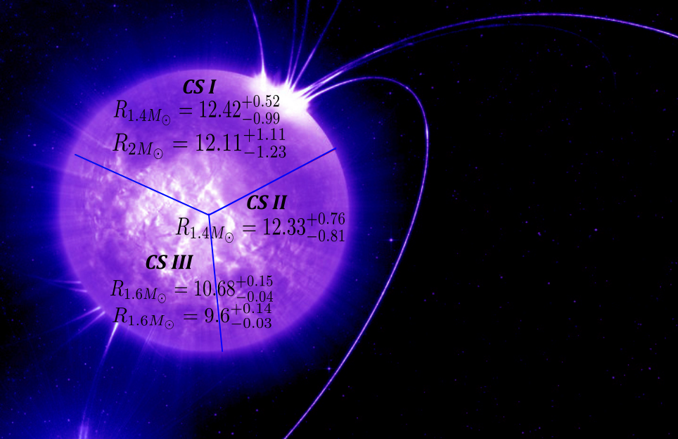
Figure 1: The constraints CSI, CSII and CSIII. This figure is inspired and based after editing on Credit: ESO/L.Calçada: https://www.eso.org/public/images/eso0831a/.

Furthermore, the important case with $\alpha=1$ is realized when $\xi\to\infty$, or similarly when $\Omega(\phi)\ll\frac{3}{2}\frac{\left(\frac{d\Omega(\phi)}{d\phi}\right)^{2}}{\omega(\phi)}$. The $R^{p}$ attractors yield a viable inflationary phenomenology, see Ref. Odintsov & Oikonomou (2022b), with the spectral index of the primordial scalar perturbations as a function of the canonical scalar field being,

$$n_{s}=\Big{(}\left(3\alpha+(3\alpha-2)p^{2}+(8-6\alpha)p-8\right)e^{2\sqrt{\frac{2}{3}}\sqrt{\frac{1}{\alpha}}\kappa\varphi}$$ (13)

$$-2(p-1)(-3\alpha+(3\alpha-2)p+8)e^{\sqrt{\frac{2}{3}}\sqrt{\frac{1}{\alpha}}\kappa\varphi}+(3\alpha-8)(p-1)^{2}\Big{)}$$

$$\times 3\alpha(p-1)^{2}\left(e^{\sqrt{\frac{2}{3}}\sqrt{\frac{1}{\alpha}}\kappa\varphi}-1\right)^{2}\,,$$

and the tensor-to-scalar ratio is,

$$r=\frac{16\left((p-2)e^{\sqrt{\frac{2}{3}}\sqrt{\frac{1}{\alpha}}\kappa\varphi}-2p+2\right)^{2}}{3\alpha(p-1)^{2}\left(e^{\sqrt{\frac{2}{3}}\sqrt{\frac{1}{\alpha}}\kappa\varphi}-1\right)^{2}}\,.$$ (14)

Also the free parameter $V_{0}$ of the potential is constrained to have values

$$V_{s}\sim 9.6\times 10^{-11}\,,$$ (15)

a results which originates from the constraints of the Planck data on the Einstein frame amplitude $\Delta_{s}^{2}$ of the scalar perturbations,

$$\Delta_{s}^{2}=\frac{1}{24\pi^{2}}\frac{V(\varphi_{f})}{M_{p}^{4}}\frac{1}{\epsilon(\varphi_{f})}\,.$$ (16)

For the purposes of this paper, we shall consider several limiting cases for the values of the parameter $\alpha$, mainly the cases $\alpha\neq 1$, and the case $\alpha=1$, which corresponds to the strong $\xi$ coupling theory. Also in order to have a viable inflationary phenomenology, the parameter $p$ which is the exponent in the $R^{p}$ attractors potential, has to take values in the range $1.91\leq p\leq 1.99$. It proves that this is irrelevant for NS studies, so we shall assume that $p=1.91$ without loss of generality. In the next section we shall specify the values of the various functions involved in the TOV equations of NS.

2 Neutron Stars with $R^{p}$ Attractors

For the purpose of studying NS in Einstein frame, we shall use the Geometrized physical units system $G=c=1$, and we shall adopt the notation of Ref. Pani & Berti (2003).

The Jordan frame scalar-tensor theory has the following form,

$$\mathcal{S}=\int d^{4}x\frac{\sqrt{-g}}{16\pi}\Big{[}\Omega(\phi)R-\frac{1}{2}g^{\mu\nu}\partial_{\mu}\phi\partial_{\nu}\phi-U(\phi)\Big{]}+S_{m}(\psi_{m},g_{\mu\nu})\,,$$ (17)

and by performing the following conformal transformation,

$$\tilde{g}_{\mu\nu}=A^{-2}g_{\mu\nu}\,,\,\,\,A(\phi)=\Omega^{-1/2}(\phi)\,,$$ (18)

we obtain the Einstein frame action,

$$\mathcal{S}=\int d^{4}x\sqrt{-\tilde{g}}\Big{(}\frac{\tilde{R}}{16\pi}-\frac{1}{2}\tilde{g}_{\mu\nu}\partial^{\mu}\varphi\partial^{\nu}\varphi-\frac{V(\varphi)}{16\pi}\Big{)}+S_{m}(\psi_{m},A^{2}(\varphi)g_{\mu\nu})\,,$$ (19)

with $\varphi$ denoting the Einstein frame canonical scalar field as in the previous section, and

$$V(\varphi)=\frac{U(\phi)}{\Omega^{2}}\,.$$ (20)

For the $R^{p}$ attractors with general $\alpha$, the important function $A(\varphi)$ has the following form,

$$A(\varphi)=e^{-\frac{1}{2}\sqrt{\frac{2}{3\alpha}}\varphi}\,,$$ (21)

therefore, the function $\alpha(\phi)$ which is defined as follows,

$$\alpha(\varphi)=\frac{d\ln A(\varphi)}{d\varphi}\,,$$ (22)

takes the form,

$$a(\varphi)=-\frac{1}{2}\sqrt{\frac{2}{3\alpha}}\,.$$ (23)

Table 1: CSI vs the $R^{p}$ Attractors for the SLy, APR and WFF1 EoSs for NS Masses $M\sim 2M_{\odot}$

$R^{p}$ Attractor Model	APR	SLy	WFF1
$\alpha=1$	$M=2.00\,M_{\odot}$	$M=2.01\,M_{\odot}$	$M=0.31\,M_{\odot}$
$\alpha=1$	$R=11.10$km	$R=11.17$km	$R=11.06$km
$\alpha=0.1$	$M=2.02\,M_{\odot}$	$M=2.00\,M_{\odot}$	$M=2.00\,M_{\odot}$
$\alpha=0.1$	$R=11.52$km	$R=11.818$km	$R=11.012$km
$\alpha=8$	$M=2.00\,M_{\odot}$	$M=2.09\,M_{\odot}$	$M=0.32\,M_{\odot}$
$\alpha=8$	$R=11.08$km	$R=10.983$km	$R=11.114$km

Finally, the Einstein frame scalar potential is given in Eq. (3), which we also quote it here for reading convenience,

$$V(\varphi)=V_{0}\,e^{-2\sqrt{\frac{2}{3\alpha}}\varphi}\left(e^{\sqrt{\frac{2}{3\alpha}}\varphi}-1\right)^{\frac{p}{p-1}}\,,$$ (24)

and in Geometrized units, the constraint on $V_{0}$ given in Eq. (15) becomes,

$$V_{0}\simeq 7.62\times 10^{-12}\,.$$ (25)

For the study of NS physics, we shall consider the following spherically symmetric metric,

$$ds^{2}=-e^{\nu(r)}dt^{2}+\frac{dr^{2}}{1-\frac{2m(r)}{r}}+r^{2}(d\theta^{2}+\sin^{2}\theta d\phi^{2})\,,$$ (26)

which describes a static NS, where the function $m(r)$ describes the total gravitational mass of the NS and $r$ stands for the circumferential radius. In the following, we shall calculate numerically the functions $\nu(r)$ and $\frac{1}{1-\frac{2m(r)}{r}}$ following a simple procedure, in which the central value of $\nu(r)$ and of the scalar field will be arbitrary and will be optimally calculated numerically by using a double shooting method.

The double shooting aims to find the optimal values of the central values of $\nu(r)$ and of the scalar field, which guarantee that the metric at numerical infinity becomes identical to the Schwarzschild metric.

Table 2: CSI vs the $R^{p}$ Attractors for the SLy, APR and WFF1 EoSs for NS Masses $M\sim 1.4M_{\odot}$

$R^{p}$ Attractors Model	APR	SLy	WFF1
$\alpha=1$	$M=0.58\,M_{\odot}$	$M=1.41\,M_{\odot}$	$M=0.25\,M_{\odot}$
$\alpha=1$	$R=11.48$km	$R=11.74$km	$R=11.89$km
$\alpha=0.1$	$M=1.39\,M_{\odot}$	$M=1.39\,M_{\odot}$	$M=0.07\,M_{\odot}$
$\alpha=0.1$	$R=11.55$km	$R=12.04$km	$R=11.79$km
$\alpha=8$	$M=0.64\,M_{\odot}$	$M=1.42\,M_{\odot}$	$M=0.28\,M_{\odot}$
$\alpha=8$	$R=11.45$km	$R=11.73$km	$R=11.46$km

This procedure is different compared to standard General Relativity (GR) NS, because in GR, the metric at the surface of the star abruptly becomes the Schwarzschild metric. This is not true in the scalar-tensor theories, because the scalar potential and the non-minimally coupling function $A(\varphi)$ have non-trivial effects on the NS beyond the surface of the star (scalarization). The Einstein frame TOV equations take the following form,

$$\frac{dm}{dr}=4\pi r^{2}A^{4}(\varphi)\varepsilon+\frac{r}{2}(r-2m(r))\omega^{2}+4\pi r^{2}V(\varphi)\,,$$ (27)

$$\frac{d\nu}{dr}=r\omega^{2}+\frac{2}{r(r-2m(r))}\Big{[}4\pi A^{4}(\varphi)r^{3}P-4\pi V(\varphi)r^{3}\Big{]}+\frac{2m(r)}{r(r-2m(r))}\,,$$ (28)

$$\frac{d\omega}{dr}=\frac{4\pi rA^{4}(\varphi)}{r-2m(r)}\Big{(}\alpha(\varphi)(\epsilon-3P)+r\omega(\epsilon-P)\Big{)}-\frac{2\omega(r-m(r))}{r(r-2m(r))}$$ (29)

$$+\frac{8\pi\omega r^{2}V(\varphi)+r\frac{dV(\varphi)}{d\varphi}}{r-2m(r)}\,,$$

$$\frac{dP}{dr}=-(\epsilon+P)\Big{[}\frac{1}{2}\frac{d\nu}{dr}+\alpha(\varphi)\omega\Big{]}\,,$$ (30)

$$\omega=\frac{d\varphi}{dr}\,,$$ (31)

with $\alpha(\varphi)$ being defined in Eq. (22). Also note that the energy density $\epsilon$ and the pressure $P$ of the matter fluid are Jordan frame quantities. We shall solve the TOV equations for both the interior and the exterior of the NS, with the following set of initial conditions being used,

$$P(0)=P_{c}\,,\,\,\,m(0)=0\,,\,\,\,\nu(0)\,,=-\nu_{c}\,,\,\,\,\varphi(0)=\varphi_{c}\,,\,\,\,\omega(0)=0\,.$$ (32)

Both $\nu_{c}$ and $\varphi_{c}$ will be determined using a double shooting method, and the numerical analysis shall be performed for three distinct piecewise polytropic EoS, with the central part being described by the SLy, WFF1 or the APR EoS.

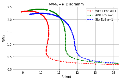
Figure 2: The $M-R$ graphs for the $R^{p}$ attractor model for the WFF1, APR and SLy EoSs, for $\alpha=1$

For the calculation of the ADM mass in the Jordan frame we shall use the following definition Odintsov & Oikonomou (2021, 2022a); Oikonomou (2021),

$$M=A(\varphi(r_{E}))\left(M_{E}-\frac{r_{E}^{2}}{2}\alpha(\varphi(r_{E}))\frac{d\varphi}{dr}\left(2+\alpha(\varphi(r_{E}))r_{E}\frac{d\varphi}{dr}\right)\left(1-\frac{2M_{E}}{r_{E}}\right)\right)\,.$$ (33)

where $r_{E}$ denotes the Einstein frame circumferential radius of the NS, and also we define $\frac{d\varphi}{dr}=\frac{d\varphi}{dr}\Big{|}_{r=r_{E}}$. Finally, the circumferential radii of the NS in the Jordan and Einstein frames are related as $R=A(\varphi(R_{s}))\,R_{s}$. We shall measure the Jordan frame mass in solar masses $M_{\odot}$ and the Jordan frame radius in kilometers.

2.1 Results of the Numerical Analysis

Let us now present the results of our numerical analysis on the NS phenomenology of the $R^{p}$ attractors. We considered three characteristic cases of attractors, corresponding to three values of $\alpha$, namely $\alpha=1$, $\alpha=0.1$ and $\alpha=8$.

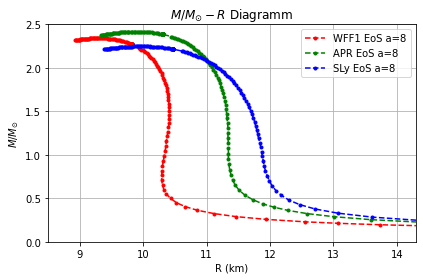
Figure 3: The $M-R$ graphs for the $R^{p}$ attractor model for the WFF1, APR and SLy EoSs, for $\alpha=8$.

All these values of $\alpha$ produce a viable inflationary phenomenology as was shown in Ref. Odintsov & Oikonomou (2022b). Here we shall present the $M-R$ graphs for the $R^{p}$ attractors for the three values of $\alpha$. Accordingly the results will be confronted with three distinct constraints on NS radii for specific mass NS. Specifically we shall use the following constraints, developed in Refs. Altiparmak, Ecker & Rezzolla (2022), Raaijmakers et al. (2021) and Bauswein, et al. (2017) to which we shall refer to as CSI, CSII and CSIII respectively. The CSI indicates that the radius of an $1.4M_{\odot}$ mass NS should be $R_{1.4M_{\odot}}=12.42^{+0.52}_{-0.99}$ and furthermore, the radius of an $2M_{\odot}$ mass NS should be $R_{2M_{\odot}}=12.11^{+1.11}_{-1.23}\,$km. Accordingly, CSII indicates that the radius of an $1.4M_{\odot}$ mass NS should be $R_{1.4M_{\odot}}=12.33^{+0.76}_{-0.81}\,\mathrm{km}$. Lastly, CSIII indicates that the radius of an $1.6M_{\odot}$ mass NS should be larger than $R_{1.6M_{\odot}}=12.42^{+0.52}_{-0.99}\,$km and the radius of a NS with maximum mass should be larger than $R_{M_{max}}>10.68^{+0.15}_{-0.04}\,$km.

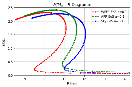
Figure 4: The $M-R$ graphs for the $R^{p}$ attractor model for the WFF1, APR and SLy EoSs, for $\alpha=0.1$.

The constraints CSI, CSII and CSIII are pictorially represented in Fig. 1. Using a double shooting LSODA python 3 numerical integration method Stergioulas (2019), and also by setting the numerical infinity at $r\sim 67.943$ km, at this point we shall present our results, which can be seen in the $M-R$ plots and the tables appearing in this work. Note that the numerical infinity plays an important role for the double shooting method, in order for the scalar field effects to be switched off at the numerical infinity.

To start with, in Figs. 2, 4 and 3 we present the $M-R$ graphs of the $R^{p}$ attractors for $\alpha=1$, $\alpha=0.1$ and $\alpha=8$ NS respectively, for the WFF1 EoS (red curve), the APR EoS (green curve) and the SLy EoS (blue curve). In all the cases, the maximum masses of the NS are larger compared to the GR case. Also it is notable that the $\alpha=1$ case is quite similar to the $\alpha=8$ case, however strong differences are observed for the $\alpha=0.1$ case.

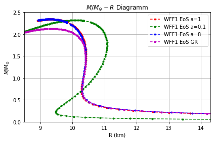
Figure 5: The $M-R$ graphs of the $R^{p}$ attractors for $\alpha=1$ (red curve), $\alpha=0.1$ (green curve), $\alpha=8$ (blue curve) and the GR (magenta curve) for the WFF1 EoS.

Also in Figs. 5, 6 and 7 we present for each EoS the $M-R$ graphs of the $R^{p}$ attractors for $\alpha=1$ (red curves), $\alpha=0.1$ (green curves), $\alpha=8$ (blue curves) and the GR (magenta curves) for the WFF1 EoS (upper left plot) the SLy EoS (upper right) and the APR EoS (bottom plot). Now let us present the confrontation of the $R^{p}$ attractor NS with the constraints CSI, CSII and CSIII.

The results of our analysis regarding the confrontation of the $R^{p}$ inflationary attractors models with the observational constraints on NS, namely CSI, CSII, AND CSIII are presented in Tables 1-5. For the case with $\alpha=1$, the SLy EoS is compatible with all the constraints, with regard to the APR, it is not compatible with CSII, the first constraint of CSI, but it is compatible with the second constraint of CSII and the CSIII constraints. Also the WFF1 case is incompatible with all the constraints. For the case with $\alpha=0.1$, the SLy EoS is compatible with all the constraints, and interestingly enough, for this case the APR is also compatible with all the constraints. However, in this case the WFF1 EoS satisfies the second constraint of CSI and also satisfies all the constraints of CSIII.

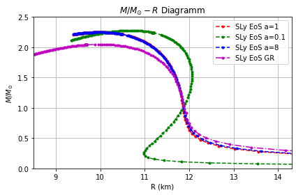
Figure 6: The $M-R$ graphs of the $R^{p}$ attractors for $\alpha=1$ (red curve), $\alpha=0.1$ (green curve), $\alpha=8$ (blue curve) and the GR (magenta curve) for the SLy EoS .

Finally, for the case with $\alpha=1$, the SLy EoS is compatible with all the constraints, with regard to the APR, it is not compatible with CSII, and the first constraint of CSI, but it is compatible with the second constraint of CSII and the CSIII constraints.

Also the WFF1 case is incompatible with all the constraints, save the first constraint of CSIII. Hence, the viable NS phenomenologies that pass all the tests imposed by the constraints CSI, CSII and CSIII, are provided by all the SLy cases for all the values of the parameter $\alpha$, and also by the APR EoS, only when $\alpha=0.1$. Thus apparently, obtaining a viable NS phenomenology nowadays is not as easy it was before the GW170817 event. Also regarding the $R^{p}$ attractors, these can be discriminated in NS, for different values of $\alpha$, especially for $0.1<\alpha<1$. However, as $\alpha$ grows larger than unity, it seems that $R^{p}$ attractors provide an almost identical NS phenomenology. This is a notable feature for the class of $R^{p}$ attractors.

Table 3: CSIII vs the $R^{p}$ Attractors for the SLy, APR and WFF1 EoSs for NS Masses $M\sim 1.6M_{\odot}$

$R^{p}$ Attractors Model	APR	SLy	WFF1
$\alpha=1$	$M=1.60\,M_{\odot}$	$M=1.60\,M_{\odot}$	$M=1.61\,M_{\odot}$
$\alpha=1$	$R=11.30$km	$R=11.63$km	$R=10.41$km
$\alpha=0.1$	$M=1.61\,M_{\odot}$	$M=1.60\,M_{\odot}$	$M=1.59\,M_{\odot}$
$\alpha=0.1$	$R=11.61$km	$R=12.05$km	$R=11.05$km
$\alpha=8$	$M=1.61\,M_{\odot}$	$M=1.60\,M_{\odot}$	$M=1.58\,M_{\odot}$
$\alpha=8$	$R=11.28$km	$R=12.05$km	$R=10.40$km

Before closing, we need to discuss an important issue, having to do with the NS phenomenology of inflationary potentials, with regard to the tidal deformability of NSs, the radial perturbations of static NSs and finally the overall stability of NSs, by also taking into account the constraints imposed by the GW170817 event. This issue however extends further from the aims and scopes of this article, since a whole article could be devoted to these issues, see for example Refs. Brown (2022) and Yang et al. (2022), in which these issues are addressed in the context of scalar-tensor gravity Brown (2022) and in unimodular gravity Yang et al. (2022).

Concluding Remarks

In this article we studied the NS phenomenology of the $R^{p}$ inflationary attractor scalar-tensor models in the Einstein frame. The $R^{p}$ attractors constitute a class of models in the Einstein frame, which originate from a large number of different models in the Jordan frame These distinct Jordan frame models result to the same phenomenology in the Einstein frame and this feature justifies the terminology inflationary attractors. Our aim was to investigate whether these attractor models can be distinguished when NSs are considered.

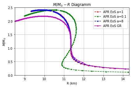
Figure 7: The $M-R$ graphs of the $R^{p}$ attractors for $\alpha=1$ (red curve), $\alpha=0.1$ (green curve), $\alpha=8$ (blue curve) and the GR (magenta curve) for the APR EoS.

As we showed the NS phenomenology corresponding to different values of the parameter $\alpha$ which characterizes the attractors, is in general different for $\alpha<1$, however the models for $\alpha>1$ show many similarities and generate almost identical $M-R$ diagrams. We also confronted the NS phenomenology of the $R^{p}$ attractors to several NS constraints, which we named CSI, CSII and CSIII. The constraint CSI was developed in Ref. Altiparmak, Ecker & Rezzolla (2022) and indicates that the radius of an $1.4M_{\odot}$ mass NS has to be $R_{1.4M_{\odot}}=12.42^{+0.52}_{-0.99}$ while the radius of an $2M_{\odot}$ mass NS has to be $R_{2M_{\odot}}=12.11^{+1.11}_{-1.23}\,$km. The constraint CSII was developed in Ref. Raaijmakers et al. (2021) and indicates that the radius of an $1.4M_{\odot}$ mass NS has to be $R_{1.4M_{\odot}}=12.33^{+0.76}_{-0.81}\,\mathrm{km}$ and the constraint CSIII was developed in Ref. Bauswein, et al. (2017) and indicates that the radius of an $1.6M_{\odot}$ mass NS has to be larger than $R_{1.6M_{\odot}}=12.42^{+0.52}_{-0.99}\,$km while the radius of the maximum mass NS has to be larger than $R_{M_{max}}>10.68^{+0.15}_{-0.04}\,$km. Our analysis indicated that for $R^{p}$ attractors, for the case with $\alpha=1$, only the SLy EoS is compatible with all the constraints, while the APR is not compatible with CSII, the first constraint of CSI, but it is compatible with the second constraint of CSII and the CSIII constraints. Also the WFF1 case is incompatible with all the constraints.

Table 4: CSII vs the $R^{p}$ Attractors for the SLy, APR and WFF1 EoSs for NS Masses $M\sim 1.4M_{\odot}$

$R^{p}$ Attractors Model	APR	SLy	WFF1
$\alpha=1$	$M=0.52\,M_{\odot}$	$M=1.41\,M_{\odot}$	$M=0.25\,M_{\odot}$
$\alpha=1$	$R=11.56$km	$R=11.74$km	$R=11.89$km
$\alpha=0.1$	$M=1.39\,M_{\odot}$	$M=1.39\,M_{\odot}$	$M=0.07\,M_{\odot}$
$\alpha=0.1$	$R=11.55$km	$R=12.04$km	$R=11.79$km
$\alpha=8$	$M=0.53\,M_{\odot}$	$M=1.42\,M_{\odot}$	$M=0.25\,M_{\odot}$
$\alpha=8$	$R=11.60$km	$R=11.738$km	$R=11.944$km

Table 5: CSIII vs the $R^{p}$ Attractors for the SLy, APR and WFF1 EoSs for Maximum NS Masses

$R^{p}$ Attractors Model	APR	SLy	WFF1
$\alpha=1$	$M=2.41\,M_{\odot}$	$M=2.24\,M_{\odot}$	$M=2.33\,M_{\odot}$
$\alpha=1$	$R=9.91$km	$R=9.99$km	$R=9.30$km
$\alpha=0.1$	$M=2.41\,M_{\odot}$	$M=2.27\,M_{\odot}$	$M=2.32\,M_{\odot}$
$\alpha=0.1$	$R=10.40$km	$R=10.09$km	$R=11.06$km
$\alpha=8$	$M=2.41\,M_{\odot}$	$M=2.27\,M_{\odot}$	$M=2.34\,M_{\odot}$
$\alpha=8$	$R=9.91$km	$R=10.72$km	$R=9.28$km

For the case with $\alpha=0.1$, which is the most interesting case phenomenologically, the SLy EoS is compatible with all the constraints, and for this case the APR is also compatible with all the constraints. However, in this case the WFF1 EoS satisfies the second constraint of CSI and also satisfies all the constraints of CSIII. Finally, for the case with $\alpha=1$, only the SLy EoS is compatible with all the constraints while the APR is not compatible with CSII, and the first constraint of CSI, but it is compatible with the second constraint of CSII and the CSIII constraints. Finally, the WFF1 case is incompatible with all the constraints, save the first constraint of CSIII. Our results indicate two main research lines, firstly that NS phenomenology for scalar-tensor theories is not easily rendered viable, since a large number of astrophysical and cosmological constraints have to be satisfied in order for the viability of the model to be guaranteed. Thus a simple parameter assigning is not the correct way to study NS nowadays, both cosmology and astrophysics constrain in a rigid way NSs. Secondly, several inflationary attractors which are indistinguishable at the cosmological level, may be discriminated to some extent when their NS phenomenology is considered. This research line is not the general rule though, so work is in progress toward comparing a large sample of cosmological attractors with respect to their NS phenomenology. Finally, let us note that the scalar-tensor inflationary framework we used in this work cannot be considered more advantageous compared to other modified gravity theories, it is one of the many possible modified gravity descriptions of the nature of NSs.

References

- LIGO & Virgo Collaboration, et al. (2017) Abbott, R., et al. 2017, PhRvL, 119, 161101
- LIGO & Virgo Collaboration, et al. (2020) Abbott, R., et al. 2020, ApJL, 896, L44
- Planck Collaboration (2020) Aghanim N., et al., 2020, A&A, 641, A6
- Akrami, et al. (2018) Akrami Y., Kallosh R., Linde A., Vardanyan V., 2018, JCAP, 06, 041
- Planck Collaboration (2020) Akrami Y., et al., 2020, A&A, 641, A10
- Akmal, Pandharipande & Ravenhall (1998) Akmal A., Pandharipande V.R., Ravenhall D.G., 1998, PhRvC, 58, 1804
- Altiparmak, Ecker & Rezzolla (2022) Altiparmak S., Ecker C. and Rezzolla L., [arXiv:2203.14974 [astro-ph.HE]].
- Antoniadis, et al. (2020) Antoniadis I., Karam A., Lykkas A., Pappas T., Tamvakis K., 2020, PoS CORFU2019, 073
- Arapoǧlu, Deliduman & Eksi (2011) Arapoǧlu A.S., Deliduman C., Eksi K. Y., 2011, JCAP, 2011, 020
- Arapoğlu, Ekşi & Yükselci (2019) Arapoğlu A.S., Ekşi K.Y., Yükselci A.E., 2019, PhRvD, 99, 064055
- Arnowitt, Deser & Misner (1960) Arnowitt R., Deser S., Misner C.W., 1960, PhRv, 118, 1100
- Astashenok, Capozziello & Odintsov (2013) Astashenok A. V., Capozziello S., Odintsov S. D., 2013, JCAP, 2013, 040
- Astashenok, Capozziello & Odintsov (2014) Astashenok A. V., Capozziello S., Odintsov S. D., 2014, PhRvD, 89, 103509
- Astashenok, Capozziello & Odintsov (2015) Astashenok A.V., Capozziello S., Odintsov S.D., 2015, JCAP, 01, 001
- Astashenok & Odintsov (2020) Astashenok A.V., Odintsov S.D., 2020, MNRAS, 498, 3616
- Astashenok, et al. (2020) Astashenok A.V., Capozziello S., Odintsov S.D., Oikonomou V.K., 2020, PhLB, 811, 135910
- Astashenok, et al. (2021) Astashenok A. V., Capozziello S., Odintsov S. D. and Oikonomou V. K., 2021, PhLB, 816, 136222, [arXiv:2103.04144 [gr-qc]].
- Bakopoulos, Kanti & Pappas (2020) Bakopoulos A., Kanti P., Pappas N., 2020, PhRvD, 101, 044026
- Bauswein, et al. (2020a) Bauswein A., et al., 2020, PhRvL, 125, 141103
- Bauswein, et al. (2020b) Bauswein A., Guo G., Lien J.H., Lin Y.H., Wu M.R., 2020, arXiv:2012.11908 [astro-ph.HE]
- Bauswein, et al. (2017) Bauswein A., Just O., Janka H.T., Stergioulas N., 2017, ApJL, 850, L34
- Baym, et al. (2018) Baym G., Hatsuda T., Kojo T., Powell P.D.,, Song Y., Takatsuka T., 2018, Rept. Prog. Phys., 81, 056902
- Biswas, et al. (2020) Biswas B., Nandi R., Char P., Bose S., Stergioulas N., 2020, arXiv:2010.02090 [astro-ph.HE]
- Blázquez-Salcedo, Scen Khoo & Kunz (2020) Blázquez-Salcedo J.L., Khoo F.S., Kunz J., 2020, EPL, 130, 50002
- Brown (2022) Brown S. M., [arXiv:2210.14025 [gr-qc]].
- Buschmann, et al. (2021) Buschmann M., Co R.T., Dessert C., Safdi B.R., 2021, PhRvL, 126, 021102
- Cai, Gong & Pi (2014) Cai Y.F., Gong J.O., Pi S., 2014, PhLB, 738, 20
- Caldwell, Kamionkowski & Weinberg (2003) Caldwell R.R., Kamionkowski M., Weinberg N.N., 2003, PhRvL, 91, 071301
- Canko, Gialamas & Kodaxis (2020) Canko D.D., Gialamas I.D., Kodaxis G.P., 2020, EPhC, 80, 458
- Capozziello, et al. (2016) Capozziello S., De Laurentis M., Farinelli R., Odintsov S.D., 2016, PhRvD, 93, 023501
- Capozziello & de Laurentis (2011) Capozziello S., de Laurentis M., 2011, PhR, 509, 167
- Carrasco, Kallosh & Linde (2015) Carrasco J.J.M., Kallosh R., Linde A., 2015, JHEP, 10, 147
- Carrasco, et al. (2015) Carrasco J.J.M., Kallosh R., Linde A., Roest D., 2015, PhRvD, 92, 041301
- Cecotti & Kallosh (2014) Cecotti S., Kallosh R., 2014, JHEP, 05, 114
- Cedeño, et al. (2019) Cedeño F.X.L., Montiel A., Hidalgo J.C., Germán G., 2019, JCAP 08, 02
- Chew, et al. (2019) Chew X.Y., Dzhunushaliev V., Folomeev V., Kleihaus B., Kunz J., PhRvD, 100, 044019
- Cuzinatto et al. (2016) Cuzinatto R. R., de Melo C. A. M., Medeiros L. G. and Pompeia P. J., Phys. Rev. D 93 (2016) no.12, 124034 , [arXiv:1603.01563 [gr-qc]].
- Dimopoulos, Wood & Owen (2018) Dimopoulos K., Wood L.D., Owen C., 2018, PhRvD, 97, 063525
- Doneva, et al. (2013) Doneva D.D., Yazadjiev S.S., Stergioulas N., Kokkotas K.D., 2013, PhRvD, 88, 084060
- Douchin & Haensel (2001) Douchin F., Haensel P., 2001, A&A, 380, 151
- Ecker & Rezzolla (2022) Ecker C., Rezzolla L., [arXiv:2209.08101 [astro-ph.HE]].
- Edwards, et al. (2020) Edwards T.D.P., Kavanagh B.J., Visinelli L. Weniger C., 2020, arXiv:2011.05378 [hep-ph]
- Ellis, Nanopoulos & Olive (2013) Ellis J., Nanopoulos D.V., Olive K.A., 2013, JCAP, 10, 009
- Faraoni & Capozziello (2010) Faraoni V., Capozziello S., 2010, Fundam. Theor. Phys., 170
- Fei, Yi & Yang (2020) Fei Q., Yi Z., Yang Y., 2020, Universe, 6, 213
- Ferrara, et al. (2013) Ferrara S., Kallosh R., Linde A., Porrati M., 2013, PhRvD, 88, 085038
- (47) Friedman, J.L., Stergioulas, N., 2013, Rotating Relativistic Stars, Cambridge University Press
- Gao, Gong & Fei (2018) Gao Q., Gong Y., Fei Q., 2018, JCAP, 05, 005
- Gao & Gong (2018) Gao Q., Gong Y., 2018, EPJP, 133, 491
- García-García, et al. (2019) García-García C., Ruíz-Lapuente P., Alonso D., Zumalacárregui M., 2019, JCAP, 07, 025
- García-García, et al. (2018) García-García C., Linder E.V., Ruíz-Lapuente P., Zumalacárregui M., 2018, JCAP, 08, 022
- Geng, Lee & Wu (2017) Geng C.Q., Lee C.C., Wu Y.P., 2017, EuPhJC, 77, 162
- Haensel, Potekhin & Yakovlev (2007) Haensel P., Potekhin A.Y., Yakovlev D.G., 2007, Astrophys. Space Sci. Libr. 326, 1
- Hebeler, et al. (2013) Hebeler K., Lattimer J.M., Pethick C.J., Schwenk A., 2013, ApJ, 773, 2013
- Hook, et al. (2018) Hook A., Kahn Y., Safdi B.R., Sun Z., 2018, PhRvL, 121, 241102
- Horbatsch, et al. (2015) Horbatsch M., et al., 2015, CQGra, 32, 204001
- Horowitz, et al. (2005) Horowitz C.J., Perez-Garcia M.A., Berry D.K., Piekarewicz J., 2005, PhRvC, 72, 035801
- Ho, et al. (2015) Ho W.C.G.,, Elshamouty K.G.,, Heinke C.O., Potekhin A.Y., 2015, PhRvC, 91, 015806
- Hwang & Noh (2005) Hwang J.C., Noh H., 2005, PhRvD, 71, 063536
- Järv, et al. (2020) Järv L., Karam A., Kozak A., Lykkas A., Racioppi A., Saal M., 2020, PhRvD, 102, 044029
- Jiang, et al. (2022) Jiang J. L., Ecker C., Rezzolla L., [arXiv:2211.00018 [gr-qc]].
- Kaiser (1994) Kaiser D.I., 1995, PhRvD, 52, 4295
- Kallosh & Linde (2013) Kallosh R., Linde A., 2013, JCAP, 07, 02
- Kallosh, Linde & Roest (2013) Kallosh R., Linde A., Roest D., 2013, JHEP, 11, 198
- Kallosh, Linde & Roest (2014b) Kallosh R., Linde A., Roest D., 2014, JHEP, 08, 052
- Kallosh, Linde & Roest (2014a) Kallosh R., Linde A. and Roest D., JHEP 09, 062, [arXiv:1407.4471 [hep-th]].
- Kallosh, Linde & Roest (2015) R. Kallosh, A. Linde and D. Roest, Phys. Rev. Lett. 112 (2014) no.1, 011303 doi:10.1103/PhysRevLett.112.011303 [arXiv:1310.3950 [hep-th]].
- Kanakis-Pegios, Koliogiannis & Moustakidis (2020) Kanakis-Pegios A., Koliogiannis P.S., Moustakidis C.C., 2020, arXiv:2012.09580 [astro-ph.HE]
- Kanfon, Mavoa & Houndjo (2020) Kanfon A.D., Mavoa F., Houndjo S.M.J., 2020, Astrophys. Space Sci., 365, 97
- Kanti, Gannouji & Dadhich (2015) Kanti P., Gannouji R., Dadhich N., 2015, PhRvD, 92, 041302
- Karam, Pappas & Tamvakis (2019) Karam A., Pappas T., Tamvakis K., 2019, JCAP, 02, 006
- Karam, Pappas & Tamvakis (2017) Karam A., Pappas T., Tamvakis K., 2017, PhRvD, 96, 064036
- Karamitsos (2019) Karamitsos S., 2019, JCAP, 09, 022
- Khadkikar, et al. (2021) Khadkikar S., Raduta A.R., Oertel M., Sedrakian A., 2021, arXiv:2102.00988 [astro-ph.HE].
- Kleihaus, Kunz & Kanti (2019) Kleihaus B., Kunz J., Kanti P., arXiv:1910.02121 [gr-qc]
- Komar (1958) Komar A., 1959, PhRvD, 113, 934
- Köppel, Bovard & Rezzolla (2019) Köppel S., Bovard L. and Rezzolla L., Astrophys. J. Lett. 872, no.1, L16 doi:10.3847/2041-8213/ab0210 [arXiv:1901.09977 [gr-qc]].
- Lattimer & Prakash (2004) Lattimer J.M., Prakash M., 2004, Science, 304, 536
- Lattimer (2012) Lattimer J.M., 2012, Ann. Rev. Nucl. Part. Sci., 62, 485
- Laurentis, Paolella & Capozziello (2015) Laurentis M., Paolella M., Capozziello S., 2015, PhRvD, 91, 083531
- Linde (2015) Linde A., 2015, JCAP, 05, 003
- Lobato et al. (2020) Lobato R., Louren O.ço, Moraes P. H. R. S., Lenzi C. H., de Avellar M., de Paula W., Dutra M. and Malheiro M., JCAP 12 (2020), 039, [arXiv:2009.04696 [astro-ph.HE]].
- Mendoza-Temis, et al. (2014) Mendoza-Temis J.J., Wu M.R., Martínez-Pinedo G., Langanke K., Bauswein A., Janka H.T., 2014, PhRvC, 92, 055805
- Miranda, et al. (2019) Miranda T., Escamilla-Rivera C., Piattella O.F., Fabris J.C., 2019, JCAP, 05, 028
- Miranda, Fabris & Piattella (2017) Miranda T., Fabris J.C., Piattella O.F., 2017, JCAP, 09, 041
- Motahar, et al. (2019) Motahar Z.A., Blázquez-Salcedo J.L., Doneva D.D., Kunz J., Yazadjiev S.S., 2019, PhRvD, 99, 104006
- Motahar, et al. (2017) Motahar Z.A., Blázquez-Salcedo J.L., Kleihaus B., Kunz J., 2017, PhRvD, 96, 064046
- Most, et al. (2018) Most E. R., Weih L. R., Rezzolla L and Schaffner-Bielich J., PhRvLet. 120 261103, [arXiv:1803.00549 [gr-qc]].
- Most, et al. (2021) Most E. R., Papenfort L. J., Tootle S. and Rezzolla L., Astrophys. J. 912, 80, [arXiv:2012.03896 [astro-ph.HE]].
- Motohashi (2015) Motohashi H., Phys. Rev. D 91 (2015), 064016, [arXiv:1411.2972 [astro-ph.CO]].
- Nathanail, Most & Rezzolla (2021) Nathanail A., Most E. R. and Rezzolla L., Astrophys. J. Lett. 908, no.2, L28, [arXiv:2101.01735 [astro-ph.HE]].
- Nojiri, Odintsov & Oikonomou (2017) Nojiri S., Odintsov S.D., Oikonomou V.K., 2017, PhR, 692, 1
- Nojiri & Odintsov (2006) Nojiri S., Odintsov S.D., 2006, Int. J. Geom. Meth. Mod. Phys., 4, 115
- Nojiri & Odintsov (2011) Nojiri S., Odintsov S. D., 2011, PhR, 505, 59
- Nozari & Rashidi (2018) Nozari K., Rashidi N., 2018, ApJ, 863, 133
- Nozari & Rashidi (2017) Nozari K., Rashidi N., 2017, PhRvD, 95, 123518
- Numajiri et al. (2022) Numajiri K., Katsuragawa T., Nojiri S., Phys. Lett. B 826 (2022), 136929 doi:10.1016/j.physletb.2022.136929 [arXiv:2111.02660 [gr-qc]].
- Nurmi, Schiappacasse & Yanagida (2021) S. Nurmi, E. D. Schiappacasse and T. T. Yanagida, [arXiv:2102.05680 [hep-ph]].
- Olmo (2011) Olmo G. J., 2011, IJMPD, 20, 413
- Odintsov & Oikonomou (2020) Odintsov S.D., Oikonomou V.K., 2020, PhLB, 807, 135576
- Odintsov & Oikonomou (2016) Odintsov S.D., Oikonomou V.K., 2016, PhRvD, 94, 124026
- Odintsov & Oikonomou (2017) Odintsov S.D., Oikonomou V.K., 2017, CQGra, 34, 105009
- Odintsov & Oikonomou (2021) Odintsov S. D. and Oikonomou V. K., Phys. Dark Univ. 32, 100805, [arXiv:2103.07725 [gr-qc]].
- Odintsov & Oikonomou (2022a) Odintsov S. D. and Oikonomou V. K., Annals Phys. 440, 168839, [arXiv:2104.01982 [gr-qc]].
- Odintsov & Oikonomou (2022b) S.D. Odintsov, V.K. Oikonomou, submitted for publication.
- Oikonomou (2021) Oikonomou V. K., Class. Quant. Grav. 38, 175005 doi:10.1088/1361-6382/ac161c [arXiv:2107.12430 [gr-qc]].
- Olmo, Rubiera-Garcia & Wojnar (2020) Olmo G. J., Rubiera-Garcia D., Wojnar A., 2020, Phys. Rept., 876, 1
- Pani & Berti (2003) Pani P., Berti E., 2014, PhRvD, 90, 024025
- Panotopoulos et al. (2021) Panotopoulos G. , Tangphati T. , Banerjee A. and Jasim M. K. , Phys.Lett.B, 817, 136330 [arXiv:2104.00590 [gr-qc]].
- Pretel et al. (2022) Pretel J. M. Z., Arbañil J. D. V., Duarte S. B., Jorás S. E. and Reis R. R. R. , [arXiv:2206.03878 [gr-qc]].
- Pretel & Duarte (2022) Pretel J. M. Z. and Duarte S. B., [arXiv:2202.04467 [gr-qc]].
- Qummer, Jawad & Younas (2020) Qummer S., Jawad A., Younas M., 2020, IJMPD, 29, 2050117
- Raaijmakers et al. (2021) Raaijmakers G., Greif S. K., Hebeler K., Hinderer T., Nissanke S., Schwenk A., Riley T. E., Watts A. L., Lattimer J. M. and Ho W. C. G., Astrophys. J. Lett. 918, L29, [arXiv:2105.06981]
- Ramazanoğlu & Pretorius (2016) Ramazanoğlu F.M., Pretorius F., 2016, PhRvD, 93, 064005
- Rashidi & Nozari (2018) Rashidi N., Nozari K., 2018, IJMPD, 27, 1850076
- Rezzolla, Most & Weih (2018) Rezzolla L., Most E. R. and Weih L. R., Astrophys. J. Lett. 852 (2018) no.2, L25, [arXiv:1711.00314 [astro-ph.HE]].
- Read, et al. (2009a) Read J.S., Lackey B.D., Owen B.J., Friedman J.L., 2009, PhRvD, 79, 124032
- Read, et al. (2009b) Read J.S., Markakis C., Shibata M., Uryu K., Creighton J.D.E., Friedman J.L., 2009, PhRvD, 79, 124033
- Renzi, Shokri & Melchiorri (2009) Renzi F., Shokri M. and Melchiorri A., Phys. Dark Univ. 27 (2020), 100450 doi:10.1016/j.dark.2019.100450 [arXiv:1909.08014 [astro-ph.CO]].
- Roest & Scalisi (2015) Roest D., Scalisi M., 2015, PhRvD, 92, 043525
- Salgado, Sudarsky & Nucamendi (1998) Salgado M., Sudarsky D., Nucamendi U., 1998, PhRvD, 58, 124003
- Safdi, Sun & Chen (2019) Safdi B. R., Sun Z., Chen A. Y., 2019, PhRvD, 99, 123021
- Sedrakian, Hayrapetyan & Shahabasyan (2006) Sedrakian D.M., Hayrapetyan M.V., Shahabasyan M.K., 2006, Astrophysics, 49, 194
- Sedrakian (2019) Sedrakian A., 2019, PhRvD, 99, 043011
- Sedrakian (2016) Sedrakian A., 2016, PhRvD, 93, 065044
- Shen, et al. (1998) Shen H., Toki H., Oyamatsu K., Sumiyoshi K., 1998, NuPhA, 637, 435
- Shibata, et al. (2014) Shibata M., Taniguchi K., Okawa H., Buonanno A., 2014, PhRvD, 89, 084005
- Shibata & Kawaguchi (2013) Shibata M., Kawaguchi K., 2013, PhRvD, 87, 104031
- Silva, et al. (2015) Silva H.O., Macedo C.F.B., Berti E., Crispino L.C.B., 2015, CQGra, 32, 145008
- Staykov, et al. (2014) Staykov K.V.,, Doneva D.D., Yazadjiev S.S., Kokkotas K.D., 2014, JCAP, 10, 006
- Steiner & Gandolfi (2012) Steiner A.W., Gandolfi S., 2012, PhRvL, 108, 081102
- Stergioulas (2019) Stergioulas Nikolaos , https://github.com/niksterg
- Tsaloukidis et al. (2022) Tsaloukidis L., Koliogiannis P. S.,Kanakis-Pegios A., Moustakidis C.C. , [arXiv:2210.15644 [astro-ph.HE]].
- Vretinaris, Stergioulas & Bauswein (2020) Vretinaris S., Stergioulas N., Bauswein A., 2020, PhRvD, 101, 084309
- Watanabe, Iida & Sato (2000) Watanabe G., Iida K., Sato K., 2000, NuPhA, 676, 455 [erratum: 2003, NuPhA, 726, 357]
- Wiringa, Fiks & Fabrocini (1988) Wiringa R.B., Fiks V., Fabrocini A., 1988, PhRvC, 38, 1010
- Xu, et al. (2009) Xu J., Chen L.W., Li B.A., Ma H.R., 2009, ApJ, 697, 1549
- Xu, Gao & Shao (2020) Xu R., Gao Y., Shao L., 2020, PhRvD, 102, 064057
- Yang et al. (2022) Yang R. X., Xie F., Liu D.J., [arXiv:2211.00278 [gr-qc]].
- Yi & Gong (2016) Yi Z., Gong Y., arXiv:1608.05922 [gr-qc]
- Yi & Gong (2018) Yi Z., Gong Y., 2019, Universe, 5, 200