AdaSfM: From Coarse Global to Fine Incremental Adaptive
Structure from Motion

Abstract

Despite the impressive results achieved by many existing Structure from Motion (SfM) approaches, there is still a need to improve the robustness, accuracy, and efficiency on large-scale scenes with many outlier matches and sparse view graphs. In this paper, we propose AdaSfM: a coarse-to-fine adaptive SfM approach that is scalable to large-scale and challenging datasets. Our approach first does a coarse global SfM which improves the reliability of the view graph by leveraging measurements from low-cost sensors such as Inertial Measurement Units (IMUs) and wheel encoders. Subsequently, the view graph is divided into sub-scenes that are refined in parallel by a fine local incremental SfM regularised by the result from the coarse global SfM to improve the camera registration accuracy and alleviate scene drifts. Finally, our approach uses a threshold-adaptive strategy to align all local reconstructions to the coordinate frame of global SfM. Extensive experiments on large-scale benchmark datasets show that our approach achieves state-of-the-art accuracy and efficiency.

I Introduction

Structure from Motion (SfM) is an important topic that has been studied intensively over the past two decades. It has wide applications in augmented reality and autonomous driving for visual localization [1, 2, 3], and in multi-view stereo [4, 5] and novel view synthesis [6] by providing camera poses and optional sparse scene structures.

Despite the impressive results from many existing works, SfM remains challenging in two aspects. The first challenge is outlier feature matches caused by the diversity of scene features, e.g. texture-less, self-similar, non-Lambertian, etc. These diverse features impose challenges in sparse feature extraction and matching which result in outliers that are detrimental to the subsequent reconstruction process. Incremental SfM [7, 8] is notoriously known to suffer from drift due to error accumulation, though is robust in handling outliers. Global SfM methods [9, 10, 11] are proposed to handle drift, but fail to solve the scale ambiguities [12] of camera positions and are not robust to outliers [13, 14].

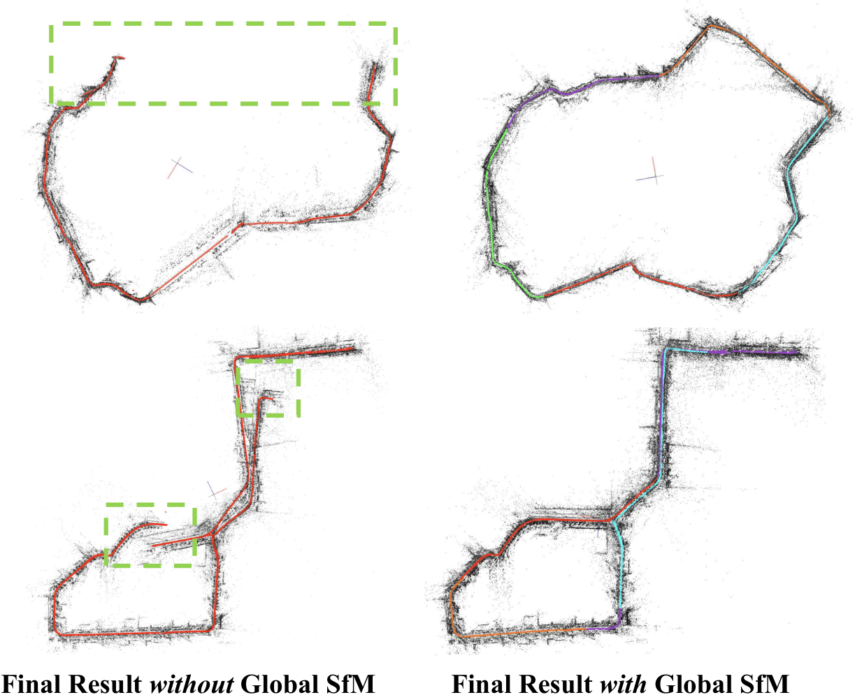
Figure 1: When combining with global SfM, our AdaSfM is more robust than traditional incremental SfM (tested on the public 4Seasons dataset [15]).

The second challenge is sparse view graphs from some large-scale datasets. Incremental SfM is known to be inefficient on large-scale datasets. Several works [16, 17, 18, 19] have been proposed to handle millions of images. These are divide-and-conquer SfM methods that deal with very large-scale datasets by grouping images into partitions. Each partition is processed by a cluster of servers that concurrently circumvents the memory limitation. However, these methods  [16, 17, 18, 19] are often limited to internet datasets or aerial images where the view graphs are very densely connected. The dense connections in the view graph ensure that there are sufficient constraints between the graph partitions. Nonetheless, divide-and-conquer methods often fail in datasets with weak associations between images for local reconstruction alignments or lack of visual constraints for stable camera registration. An example of such a dataset is autonomous self-driving cars where the interval between consecutive images can be large.

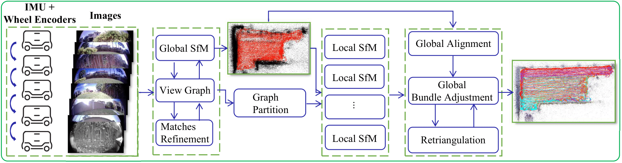
Figure 2: The pipeline of our proposed SfM method. Our method takes images and measurements from low-cost sensors as inputs. The view graph is built after feature matching and refined by the result of global SfM. The absolute poses from the global SfM are used as priors in the subsequent local SfM process. The final reconstruction result is merged into the global SfM reference frame.

In view of the challenges from the outlier feature matches and sparse view graphs on the existing SfM approaches, we propose AdaSfM: a coarse-to-fine adaptive SfM pipeline to enhance the robustness of SfM in dealing with large-scale challenging scenes. Specifically, we first solve the global SfM at a coarse scale, and then the result of the global SfM is used to enhance the scalability of the local incremental reconstruction. Both the scale ambiguities and outlier ratio in global SfM can be significantly reduced by incorporating measurements from the IMU and wheel encoder, which are often available in mobile devices or autonomous self-driving cars. We preintegrate [20] the IMU measurements to get the relative poses of consecutive frames $\mathcal{P}_{t}=\{\mathbf{P}_{t_{0}},\mathbf{P}_{t_{1}},\cdots\}$, and use the measurements from the wheel encoder to constrain scale drifts of the IMU preintegration [21]. We then replace the relative poses of the consecutive frames in the view graph formed by two-view geometry [22, 8] with $\mathcal{P}_{t}$ estimated by the IMU and wheel encoder. This augmented view graph is then used to estimate the global poses. Consequently, we obtain a coarse scene structure and camera poses, where the latter can be used to filter wrong feature matches. Since that, we partition the view graph with the existing graph cut method [23] and then extend the sub-graphs with a novel adaptive flood-fill method to enhance the constraints of separators [24]. We define separators as images that connect different sub-graphs. For each local SfM, the poses from the global SfM are used for camera registration and to constrain the global refinement of 3D points and camera poses. Finally, we design an adaptive global alignment strategy to merge local reconstructions with the coordinate frame of the global SfM set as the reference frame. We illustrate the pipeline of our method in Fig. 2.

We evaluate our method extensively on large-scale challenging scenes. Experimental results show that our AdaSfM is adaptive to different scene structures. Furthermore, we achieve better robustness and comparable efficiency in comparison to existing state-of-the-art SfM methods.

II Related Work

Incremental SfM. Agarwal et al. [7] apply preconditioned conjugate gradient [25] to accelerate large-scale BA [26]. The drift problem is alleviated in [27] with a re-triangulation (RT) step before global BA. Schönberger and Frahm [8] augment the view graph by estimating multiple geometric models in geometric verification and improve the image registration robustness with next best view selection. In addition to the RT before BA [27], RT is also performed after BA in [8]. To reduce the time complexity of repetitive image registration, Cui et al [28] select a batch of images for registration, and select a subset of good tracks for BA.

Global SfM. The simplest configuration of a global SfM method only requires 1) estimating the global rotations by rotation averaging (RA), 2) obtaining the global positions by TA, and 3) triangulating 3D points and performing a final global BA. Govindu [29] represents rotations by lie-algebra, and global rotations and global positions are estimated simultaneously. Chatterjee and Govindu [30, 31] improve the rotation estimation of  [29] by a robust $l_{1}$ initialization followed by a refinement of the rotations with iteratively reweighted least-squares (IRLS) [32]. To solve the TA problem, Wilson et al [33] project relative translations onto the 1D space to identify outliers. Relative translations that are inconsistent with the translation directions that have the highest consensus are removed. A nonlinear least-squares problem is then solved to get the global positions. Goldstein et al. [34] relax the scale constraints of  [33] to linear scale factors, and the convex linear programming problem is solved by ADMM [35]. Özyesil and Singer [12] utilize the parallel rigidity theory to select the images where positions can be estimated uniquely and solved as a constrained quadratic programming problem. By minimizing the $\sin\theta$ between two relative translations, Zhuang et al. [36] improve the insensitivity to narrow baselines of TA. The robustness of TA is also improved in [36] by incorporating global rotations.

Hybrid SfM. Cui et al. [37] obtain orientations by RA and then register camera centers incrementally with the perspective-2-point (P2P) algorithm. Bhomick et al. [16] propose to divide the scene graph, where the graph is built from the similarity scores between images. Feature matching and local SfM can then be executed in parallel and local reconstructions are merged [16]. Zhu et al. [18, 19] adopt a similar strategy to divide the scene and the graph is constructed after feature matching. The relative poses are collected after merging all local incremental reconstruction results. The outliers are filtered during local reconstruction, global rotations are fixed by RA, and camera centers are registered with TA at the cluster level. Based on [18], Chen et al. [17] find the minimum spanning tree (MST) to solve the final merging step. The MST is constructed at the cluster level, and the most accurate similarity transformations between clusters are given by the MST. Locher et al. [38] filtered wrong epipolar geometries by RA before applying the divide-and-conquer method [18]. Jiang et al. [39] use a visual-inertial navigation system (VINS)  [40] to first estimate the camera trajectories with loop detection and loop closure  [41]. Images are then divided into sequences according to timestamps. However, [39] requires two carefully designed systems: one for VINS with loop detection and the other for SfM. Loop detection is also a challenge in real-world scenes.

III Notations

We denote the absolute camera poses as $\mathcal{P}=\{\mathbf{P}_{i}=[\mathbf{R}_{i}|\mathbf{t}_{i}]\}$, where $\mathbf{R}_{i},\mathbf{t}_{i}$ are the rotation and translation of the $i$-th image, respectively. The absolute camera poses project 3D points $\mathcal{X}=\{\mathbf{X}_{k}\}$ from the world frame to the camera frame. The camera centers are denoted by $\{\mathbf{C}_{i}\}$. The relative pose from image $i$ to image $j$ are denoted as $\mathbf{P}_{ij}=[\mathbf{R}_{ij}|\mathbf{t}_{ij}]$, where $\mathbf{R}_{ij},\mathbf{t}_{ij}$ are the relative rotations and translations, respectively. We define the view graph as $\mathcal{G}=\{\mathcal{V},\mathcal{E}\}$, where $\mathcal{V}$ denotes the collection of images and $\mathcal{E}$ denotes the two view geometries, i.e. the relative poses and inlier matches between the image pairs. For two rotations $\mathbf{R}_{i},\mathbf{R}_{j}$, we use $\log(\mathbf{R}_{i},\mathbf{R}_{j})=\log(\mathbf{R}_{j}\mathbf{R}_{i}^{\top})$ to denote the angular error and $\|\mathbf{R}_{i}-\mathbf{R}_{j}\|_{F}$ to denote the chordal distance. Additionally, the keypoints and the normalized keypoints after applying the intrinsic matrix $\mathbf{K}$ are denoted by $\mathbf{u}$ and $\mathbf{\hat{u}}$, respectively.

IV Coarse Global to Fine Incremental SfM

In this section, we introduce our method in detail. In Sec. IV-A, we introduce our global SfM that can effectively cope with outliers in challenging scenes. A refinement step is also introduced to remove outlier matches after global SfM. In Sec. IV-B, we describe our parallel incremental SfM approach that utilizes the results from coarse global SfM to mitigate the problems from sparse view graphs.

IV-A Coarse Global SfM

We first obtain the absolute rotations $\mathbf{R}_{i}$ by solving the rotation averaging problem:

$$\operatorname*{arg\,min}_{\{\hat{\mathbf{R}}_{i}\}}\ \sum_{i\in\mathcal{V},\atop(i,j)\in\mathcal{E}}d(\hat{\mathbf{R}}_{j}\hat{\mathbf{R}}_{i}^{\top},\mathbf{R}_{ij}),$$ (1)

where $\hat{\mathbf{R}}_{i}$ denotes the absolute poses obtained by rotation averaging, and $d(\cdot)=\|\cdot\|_{F}$ denotes the chordal distance. Eq. (1) can be solved robustly and efficiently by [42]. We then obtain the absolute camera positions by solving the translation averaging problem. However, existing translation averaging methods often fail to recover the camera positions under challenging scenes due to two main factors: 1) The high ratio of outliers in the relative translations. 2) The view graph is solvable only when the parallel rigid graph condition [12] is satisfied. To alleviate the first problem, we first remove the erroneous matching pairs by checking the discrepancy of relative rotations: $\log(\mathbf{R}_{ij}^{\top}\hat{\mathbf{R}}_{j}\hat{\mathbf{R}}_{i}^{\top})>\epsilon_{\mathbf{R}}$, and then the relative translations [12] are refined in parallel by:

$$\operatorname*{arg\,min}_{\mathbf{t}_{ij}}\ \|\hat{\mathbf{u}}^{\prime\top}([\mathbf{t}_{ij}]_{\times}(\hat{\mathbf{R}}_{j}\hat{\mathbf{R}}_{i}^{\top}))\hat{\mathbf{u}}\|,\quad\text{s.t.}\quad\|\mathbf{t}_{ij}\|=1.$$ (2)

We do not extract the rigid parallel graph [12] to solve the scale ambiguities since it is time-consuming to solve polynomial equations. Furthermore, the state-of-the-art method to establish the solvability of a view graph is only limited to 90 nodes [43]. We improve the solvability of the view graph by augmenting the relative translations in $\mathcal{P}_{t}$ of the consecutive frames from the IMU and wheel encoder. We do not augment the relative rotations because they are more accurate from the image-based two-view geometry. Note that errors can accumulate increasingly in the augmented relative poses during the motion of the devices due to the bias of the accelerometers and gyroscopes in the IMU, and drifts in the wheel encoder caused by friction and wheel slippages. To circumvent this problem, we only use the relative poses where the time difference is below a threshold $\epsilon_{T}$.

Since we obtained the augmented view graph $\mathcal{G}_{\text{aug}}=\{\mathcal{V},\mathcal{E}_{\text{aug}}\}$, the rigidity of the original view graph is augmented and the scale ambiguities of some images can be eliminated. We can then further solve the translation averaging problem below:

$$\operatorname*{arg\,min}_{\begin{subarray}{c}\hat{\mathbf{C}}_{i},i\in\mathcal{V};\atop~{}s_{ij},(i,j)\in\mathcal{E}_{\text{aug}}\end{subarray}} \sum_{(i,j)\in\mathcal{E}_{\text{aug}}}\|s_{ij}(\hat{\mathbf{C}}_{i}-\hat{\mathbf{C}}_{j})-\mathbf{R}_{j}^{\top}\mathbf{t}_{ij}\|,$$ (3)

s.t. $$s_{ij}\geq 0,\quad\forall(i,j)\in\mathcal{E}_{\text{aug}};\quad\sum_{i\in\mathcal{V}}\hat{\mathbf{C}}_{i}=0.$$

(3) can be solved efficiently and robustly under the $l_{1}$-norm by collecting all the constraints. Note all the relative translations are normalized in $\mathcal{E}_{\text{aug}}$. The right of Fig. 3 shows our global SfM result by solving (3).

After translation averaging, we triangulate the 3D points and perform an iterative global bundle adjustment to refine camera poses. It is worth mentioning that, global SfM can generate more tracks than incremental SfM, as its camera poses are less accurate and thus it fails to merge some tracks that are physically the same. Besides, according to [28], tracks are redundant for optimisation. Therefore, we can reduce the computation and memory burden with fewer tracks. Though a well-designed algorithm may help with the selection of tracks, we simply create tracks with a stricter threshold: only when the angle between the two rays respectively go through the 3D point and the two camera centers are larger than 5 degrees, it is deemed as a valid track. Note that for numerical stability during optimization, the coordinates are normalized after each iteration.

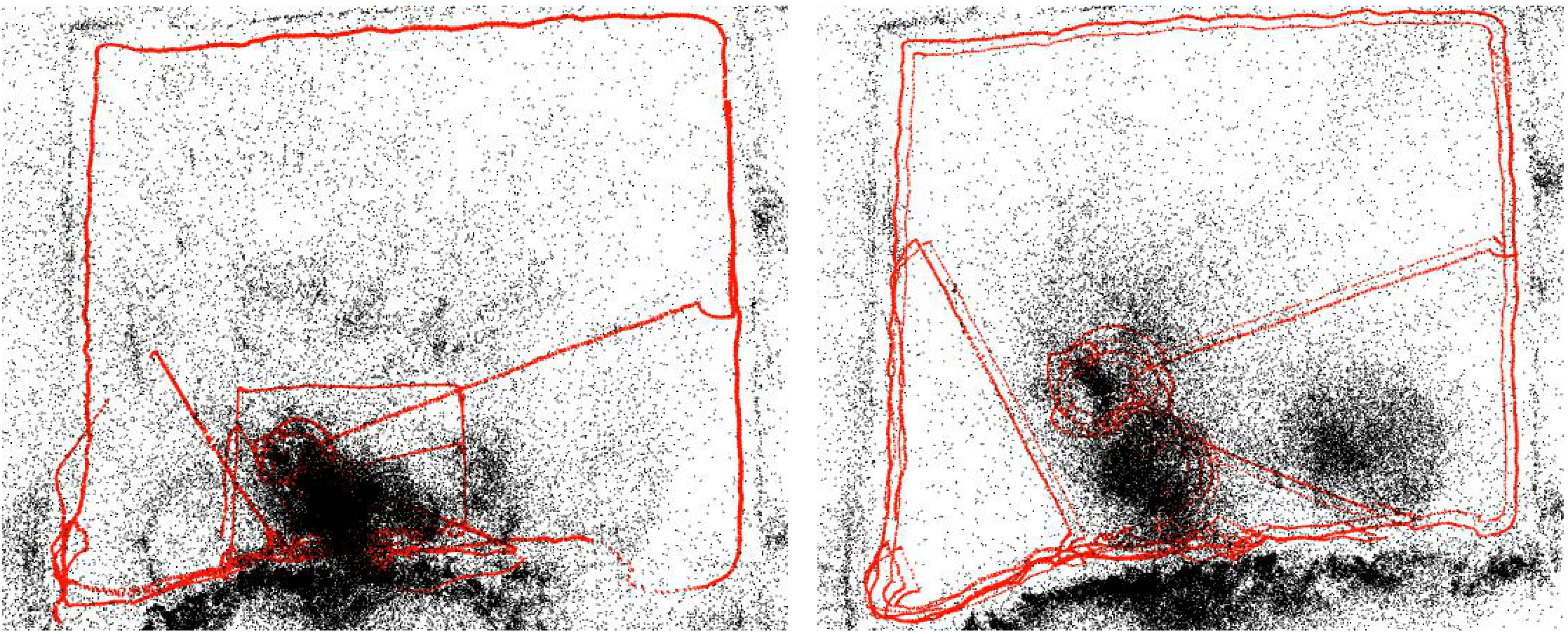
Figure 3: Comparison of global SfM results. Results from  [12] (left) and Eq. (3) (right). Red and black colors respectively denote vehicle trajectories and sparse point clouds.

IV-A1 Matches Refinement

The correct camera poses recovered by our global SfM with the relative poses from the low-cost sensors to eliminate the wrong two-view geometry estimates can be further utilized to filter out wrong image feature matches. For a calibrated camera with known intrinsics, we can recover the essential matrix between images i and j from $\hat{\mathbf{E}}=[\hat{\mathbf{t}}_{ij}]_{\times}\hat{\mathbf{R}}_{ij}$ with the absolute rotations $\hat{\mathbf{R}}_{i}$ and translations $\hat{\mathbf{t}}_{i}$ computed from rotation and translation averaging. $(\hat{\mathbf{t}}_{ij},\hat{\mathbf{R}}_{ij})$ are computed from $(\hat{\mathbf{R}}_{i},\hat{\mathbf{R}}_{j})$ and $(\hat{\mathbf{t}}_{i},\hat{\mathbf{t}}_{j})$. The true matches $\hat{\mathbf{u}}^{\prime}\leftrightarrow\hat{\mathbf{u}}$ must satisfy the check on the total point-to-epipolar line distance [22] over the two views, i.e.

$$d_{\bot}(\hat{\mathbf{u}},\mathbf{E}\hat{\mathbf{u}}^{\prime})+d_{\bot}(\hat{\mathbf{u}}^{\prime},\mathbf{E}\hat{\mathbf{u}})\leq\epsilon_{M}.$$ (4)

$d_{\bot}(\mathbf{x},\mathbf{l})$ gives the shortest distance between a point $\mathbf{x}$ and a line $\mathbf{l}$. The epipolar lines on the two images are given by $\mathbf{l}=\mathbf{E}\hat{\mathbf{u}}^{\prime}$ and $\mathbf{l}^{\prime}=\mathbf{E}\hat{\mathbf{u}}$. $\epsilon_{M}$ is the threshold for the check.

The effectiveness of global SfM to filter wrong matches can be seen in Fig. 7. We build a pseudo ground truth by COLMAP [8] to evaluate the accuracy of the global SfM. The ratio test is performed after NN by default. Fig. 4 shows the inlier ratio distribution after NN+RANSAC and matches refinement with relative poses obtained from global SfM and incremental SfM, respectively. Table. I gives the relative pose estimation AUC of NN+RANSAC and global SfM with respect to incremental SfM. It can be seen that our coarse global SfM can obtain comparable accuracy to COLMAP [8] in the refinement of the matches.

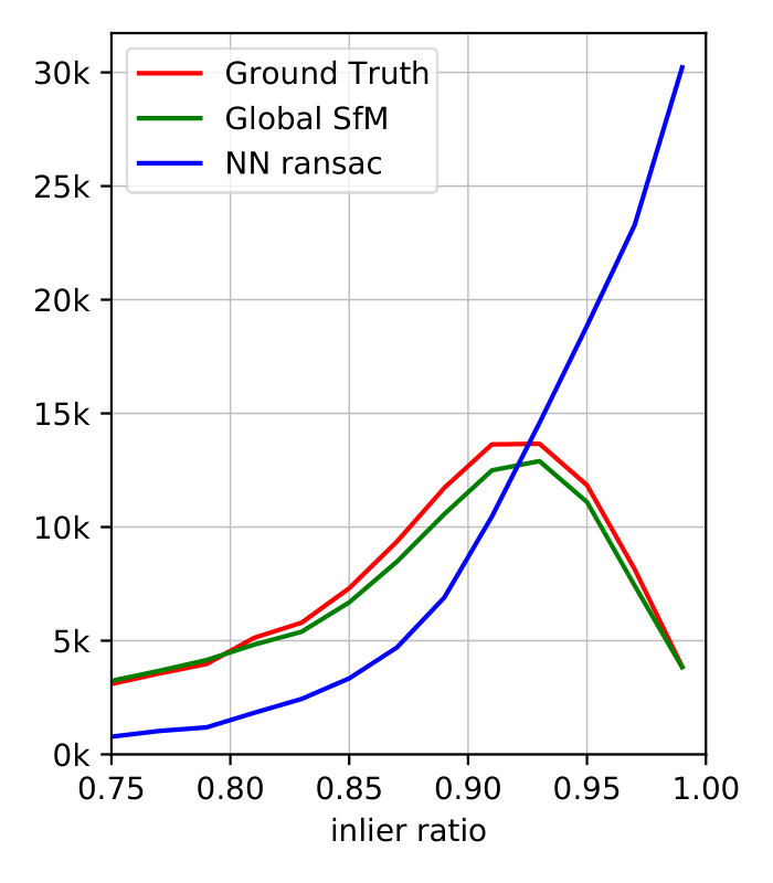
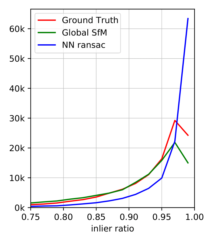
Figure 4: Inlier ratio distribution of NN+RANSAC, global SfM and
incremental SfM (ground truth) on the 711 (left) and B6 (right) datasets.

AUC	NN+RANSAC		Global SfM		NN+RANSAC		Global SfM
	$\mathbf{R}$	$\mathbf{t}$	$\mathbf{R}$	$\mathbf{t}$	$\mathbf{R}$	$\mathbf{t}$	$\mathbf{R}$	$\mathbf{t}$
$\text{@}0.1^{\circ}$	1.52	0.01	6.67	0.02	2.14	0.01	8.41	0.09
$\text{@}0.5^{\circ}$	14.74	0.25	44.87	0.48	21.47	0.36	44.14	1.96
$\text{@}1.0^{\circ}$	28.92	0.96	64.15	1.80	40.99	1.40	64.48	6.48
$\text{@}3.0^{\circ}$	55.75	5.85	84.76	9.60	68.08	9.18	86.89	24.00
$\text{@}5.0^{\circ}$	68.27	10.94	90.34	17.71	77.39	17.58	92.06	35.41
$\text{@}10.0^{\circ}$	81.71	20.21	94.99	33.03	86.81	32.46	96.01	51.07
$\text{@}20.0^{\circ}$	90.29	29.97	97.48	49.87	92.90	46.95	98.00	64.65

TABLE I: Relative pose estimation AUC of NN+RANSAC and global SfM with respect to incremental SfM on the B6 (column 2-5) and 711 (column 6-9) datasets.

IV-B Finer Parallel Incremental SfM

Although we have obtained the absolute camera poses by global SfM, these coarse poses are not accurate enough for localization. To improve the accuracy, we propose to refine the camera poses and scene structure with the divide-and-conquer incremental SfM.

IV-B1 Adaptive Graph Partition

Existing approaches [18, 17] used a cut-and-expand schema to create overlapping areas between partitions. However, these approaches have two main drawbacks: : 1) The overlapping areas are not enough for final merging when the view graph becomes too sparse. This can be seen from Fig. 5(a). Edges (3, 20), (7, 9), (8, 9), (8, 20), (16, 19), (17, 18) are collected after the graph cut, and then the images on these edges are added as separators of the partitions. In Fig. 5(a), only images $\{3,7,8,9,16,17,18,19,20\}$ can be used to create the overlapping areas (Fig. 5(b)). However, these separator images are insufficient to compute the similarity transformations for merging all local reconstructions due to the sparsity of the view graph. 2) Graph cut tends to separate partitions along edges with weak associations. This means the separators are often weakly constrained during reconstruction and thus their poses might not be accurate enough during reconstruction.

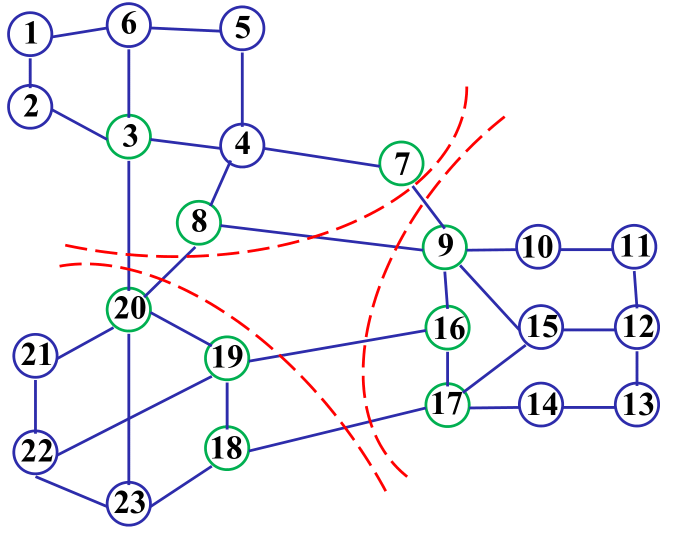
(a) Initial graph cut.

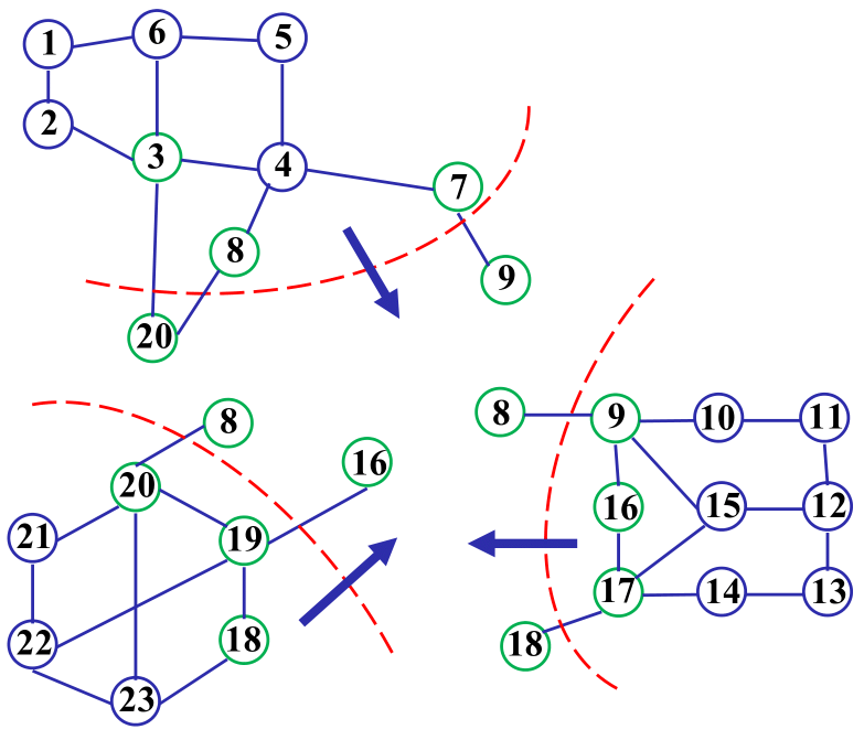
(b) The 1st graph expansion.

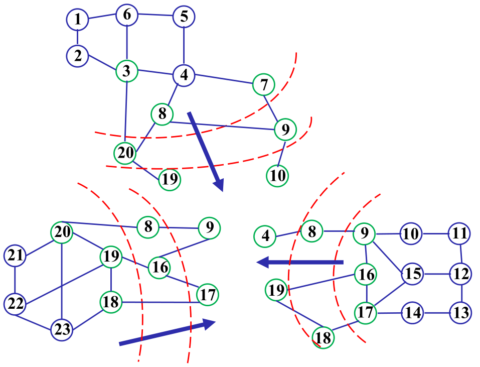
(c) The 2nd graph expansion.

Figure 5: Pipeline of adaptive flood-fill graph partition. In the view graph, nodes are denoted by blue circles, edges are denoted by blue solid lines. Separators are marked by green circles.

We propose a flood-fill graph partition algorithm to overcome the above-mentioned disadvantages. We refer to the added nodes in each cluster after an expansion operation as a layer. The separators are collected to form a layer after the graph cut on the complete view graph. Fig. 5(a) shows examples of the separators marked green. We have separators $\mathcal{S}_{1}=\{\{3,7,8\},\{9,16,17\},\{18,19,20\}\}$ in the first layer. We then collect all the adjacent images of every separator for each partition. We find one adjacent image that does not belong to partition $k$, and add it to the second layer of separators $\mathcal{S}_{2}$ in partition $k$. Adjacent images are sorted in descending order according to the weights of the edges, i.e. the number of inlier matches. Fig. 5(b) shows that the separators $\mathcal{S}_{2}=\{\{9,20\},\{8,18\},\{8,16\}\}$ at the second layer after traversing all separators in $\mathcal{S}_{1}$. The expansion step is repeated until the number of overlapping images reaches the overlapping threshold $\tau_{\text{ot}}$ (e.g. 30$\%$).Fig. 5(c) shows the separators $\mathcal{S}_{3}$ at the third layer.

IV-B2 Local Incremental SfM

We perform incremental SfM in parallel after graph partitioning. For local incremental SfM, we utilize the result of global SfM $\hat{\mathcal{P}}_{\text{global}}$ to improve the robustness of the image registration step, and to further constrain the camera poses during global optimization.

Image Registration

We follow [8] for the two-view initialization. We then select a batch of the next-best images to register, where any image that sees at least $v_{p}$ scene points are put into one batch and sorted in descending order. For each candidate image $i$, we first use the P3P [44] to compute the initial pose $\mathbf{P}_{i}^{\text{p3p}}$. However, images can be registered wrongly due to wrong matches or scene degeneration. We propose to also compute the image pose $\mathbf{P}_{i}^{\text{gb}}=[\mathbf{R}_{i}^{\text{gb}}\mid\mathbf{t}_{i}^{\text{gb}}]$ using $\hat{\mathcal{P}}_{\text{global}}$. We first collect the set of registered images that are co-visible to image $i$, and then the rotation of image $i$ can be computed by a single rotation averaging [45]:

$$\operatorname*{arg\,min}_{\mathbf{R}_{i}^{\text{gb}}} \sum_{k}\|\log(\hat{\mathbf{R}}_{ki}\mathbf{R}_{k},\mathbf{R}_{i}^{\text{gb}})\|,\quad\text{where}\quad\hat{\mathbf{R}}_{ki}=\hat{\mathbf{R}}_{i}\hat{\mathbf{R}}_{k}^{\top},$$ (5)

where $k$ is the index of images that are co-visible to image $i$. For image translation, we first compute the translation of image $i$ by each co-visible image and simply adopt the median of each dimension in translations $\mathbf{t}_{i}^{\text{gb}}$:

$$\mathbf{t}_{i}^{\text{gb}}=\text{median}\{\hat{\mathbf{t}}_{ki}+\hat{\mathbf{R}}_{ki}\mathbf{t}_{k}\},\quad\text{where}\quad\hat{\mathbf{t}}_{ki}=\hat{\mathbf{t}}_{i}-\hat{\mathbf{R}}_{ki}\hat{\mathbf{t}}_{k}.$$ (6)

To select the best initial pose, we reproject all visible 3D points of image $i$ to compute the reprojection errors and mark the 3D point with the reprojection error less than 8px as an inlier. Finally, we select the pose which has the most inliers.

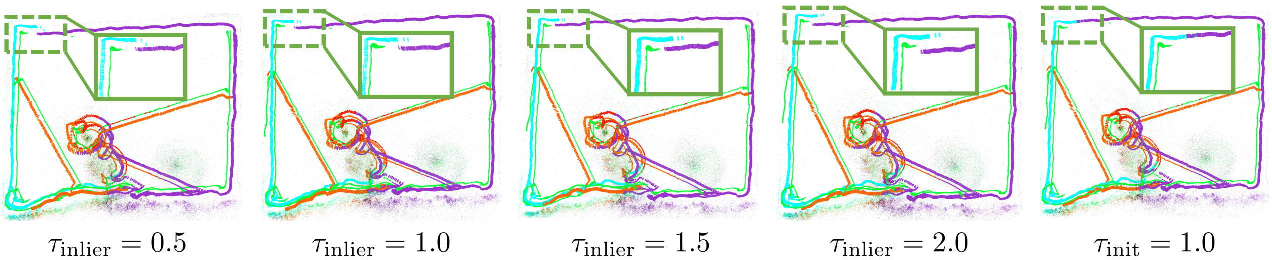
Figure 6: Vehicle trajectories of different threshold trials when merging sub-reconstructions. The last figure is obtained by our method which starts from an initial inlier threshold $\tau_{\text{init}}$. Others are the results of using a fixed threshold during the alignment to merge all local reconstructions.

Bundle Adjustment

To alleviate the drift problem for local incremental SfM, we perform global optimization using the classical bundle adjustment with the absolute poses obtained from global SfM as the supervision for the incrementally registered poses, i.e.

$$\operatorname*{arg\,min}_{\mathbf{R},\mathbf{C},\mathbf{X}} \Big{\{}\sum_{i}\sum_{k}\|\mathbf{\Pi}(\mathbf{R}_{i},\mathbf{C}_{i},\mathbf{X}_{k})-\mathbf{u}_{ik}\|~{}~{}~{}+$$ (7)

$$\sum_{(i,j)\in\mathcal{E}_{\text{aug}}}\Big{(}\|\log(\mathbf{R}_{ij},\hat{\mathbf{R}}_{ij}\|+d_{\angle}(\mathbf{t}_{ij},\hat{\mathbf{t}}_{ij})\Big{)}\Big{\}},$$

where $\mathbf{\Pi}(\cdot)$ reprojects a 3D point back to the image plane, $d_{\angle}(\cdot)$ denotes the angle between two vectors. Note that we do not make the hard constraint to force the translation part of $\hat{\mathbf{P}}_{ij}^{-1}\mathbf{P}_{ij}$ to be a zero-vector. Instead, we use $d_{\angle}(\mathbf{t}_{ij},\hat{\mathbf{t}}_{ij})=d_{\angle}(\mathbf{C}_{i}-\mathbf{C}_{j},\hat{\mathbf{C}}_{i}-\hat{\mathbf{C}}_{j})$ to constrain the translation direction of camera poses. This is because the absolute positions obtained from global SfM are not sufficiently accurate.

IV-B3 Adaptive Global Alignment

The global alignment step is crucial for the divide-and-conquer SfM since a wrong similarity transformation can cause catastrophic failure of the reconstruction. The difficulties in estimating a reliable similarity transformation are due to 1) The existence of outliers in registered camera poses. Although the outliers can be identified by RANSAC [46], the threshold that indicates outliers is hard to determine. This is due to the loss of the absolute scale of the real world in SfM without additional information such as GPS. It indicates that the optimal outlier threshold varies for each cluster. 2) The estimated similarity transformation can overfit wrongly with insufficient sample points. Existing divide-and-conquer methods  [16, 18, 19, 47, 17] suffer from the two issues because the similarity transformations can only be estimated from the overlapping areas between the pairwise local partitions.

To tackle the first issue, we propose an adaptive strategy to determine the inlier threshold $\tau_{\text{inlier}}$. Given an initial inlier threshold $\tau_{\text{init}}$, we first estimate the similarity transformation by RANSAC [46]. We then compute the inlier ratio $r_{\text{inlier}}$ and increase the inlier threshold if $r_{\text{inlier}}<r_{\min}$. Furthermore, we decrease the threshold if $r_{\text{inlier}}\geq r_{\max}$ to prevent the threshold from becoming too large. A large threshold allows more outliers to be falsely selected and thus harming the similarity transformation estimation. The second issue can be solved easily within our framework. We set the coordinate frame of the global SfM as the reference frame, and align each local SfM into the reference frame. Therefore, for each partition, we can have as many sample points as the number of common registered images between a global SfM and a local partition to compute the similarity transformation. We also show the effectiveness of the algorithm to merge local reconstructions in Fig. 6. When zooming in, we can observe that our adaptive strategy perfectly closed the loop while other fixed threshold trials failed.

V Experimental Results

In this section, we perform extensive experiments to demonstrate the accuracy, efficiency, and robustness of our proposed methods.

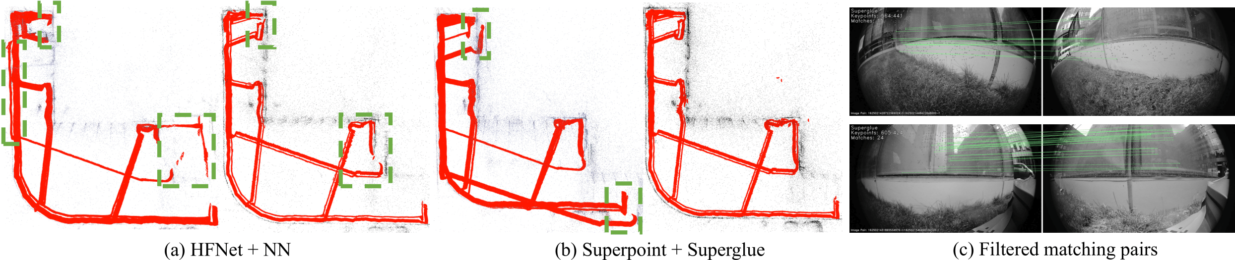
Figure 7: Vehicle trajectories after match refinement on B6 dataset. In Fig.(a) and Fig.(b), the visual results are respectively reconstructed without (left) and with (right) match refinement in each sub-figure. Fig.(c) shows some of the wrong matching pairs that are filtered by our method.

Dataset	$N$	COLMAP [8]					GraphSfM [17]					Ours(Global SfM)				Ours(Global+Inc.)
		$N_{c}$	$N_{p}$	$\bar{L}$	RMSE	$T$	$N_{c}$	$N_{p}$	$\bar{L}$	RMSE	$T$	$N_{c}$	$N_{p}$	$\bar{L}$	$T$	$N_{c}$	$N_{p}$	$\bar{L}$	RMSE	$T$
high free	48,753	48,733	567,030	21.59	1.47	597,171	48,491	540,711	22.73	1.38	88,896 ($\times 6.7\uparrow$)	48,758	521,080	14.51	5,177	48,694	540,942	22.79	1.66	105,163 ($\times 5.7\uparrow$)
711	29,619	27,175	303,352	25.35	1.64	160,322	29,618	259,292	33.37	1.46	33,514 ($\times 4.8\uparrow$)	29,629	249,673	18.86	3,499	29,619	256,495	33.79	1.61	38,682 ($\times 4.1\uparrow$)
yht	7,472	7,470	90,437	20.81	1.16	20,428	6,709	78,659	20.58	1.17	7,526 ($\times 2.7\uparrow$)	7,472	132,167	13.67	524	7,472	108,711	17.35	1.43	9,778 ($\times 2.1\uparrow$)
A4	5,184	5,132	33,694	41.92	1.69	18,104	4,285	28,726	49.79	1.55	12,670 ($\times 1.4\uparrow$)	5,184	24,193	26.59	1,349	5,184	34,007	48.30	1.43	6,924 ($\times 2.6\uparrow$)
Htbd	14,651	14,645	231,870	24.62	1.30	56,888	14,645	232,441	24.25	1.37	17,187 ($\times 3.3\uparrow$)	14,646	190,904	23.47	1,523	14,646	238,035	23.76	1.36	16,852 ($\times 3.4\uparrow$)
jy1	32,484	32,463	534,117	20.57	1.44	346,161	32,466	536,331	20.18	1.52	28,673 ($\times 12.1\uparrow$)	32,484	463052	16.12	3,077	32,466	621,437	17.77	1.53	33,555 ($\times 10.3\uparrow$)

TABLE II: Comparison of runtime and accuracy on real-world datasets. For runtime $T$ (seconds), the first, second and third The best results are highlighted in color. $N_{c},N_{p}$ denote the number of registered images and 3D points, respectively, $\bar{L}$ denotes the average track length , and RMSE denotes the root mean square error in pixel.

V-A Implementation Details

We use HFNet [48] as the default feature extractor and use the NN search for matching. A maximum of 500 feature points are extracted from each image and matched to the top 30 most similar images based on the global descriptors from HFNet. We assume cameras are pre-calibrated and use the ceres-solver [49] for bundle adjustment. We did not compare our method against [39], as VINs [40] fails to find the right loops in our datasets. All methods are run on the same computer with 40 CPU cores and 96 GB RAM.

Evaluation Datasets: We evaluate our method on our self-collected outdoor datasets and the 4seasons [15] datasets. Our self-collected datasets are collected by low-speed autonomous mowers, of which the running environments have many plants and texture-less areas. The 4seasons dataset is a cross-season dataset that includes multi-sensor data such as IMU, GNSS, and stereo images. It also provides camera poses computed by VI-Stereo-DSO [50, 51] and ground-truth camera poses by fusing multi-sensor data into a SLAM system. See our attached video for a more qualitative and quantitative evaluation of the 4Seasons dataset.

Running Parameters: Empirically, we use the time threshold $\epsilon_{T}=500~{}\text{ms}$ to adopt the fused relative poses in $\mathcal{G}_{\text{aug}}$, and $\epsilon_{\mathbf{R}}=5~{}\text{degree}$ to check to relative rotation discrepancy. The point-to-epipolar line distance is $\epsilon_{M}=4~{}\text{px}$. Besides, we set the overlapping ratio $\tau_{\text{ot}}=0.3$ in the graph partition, $v_{p}=10$ for an image to be a candidate to register, and $r_{\min}=0.7,r_{\max}=0.9,\tau_{\text{init}}=1.0,\alpha_{\text{inc}}=0.2,\alpha_{\text{dec}}=0.1$ in global alignment.

V-B How Matching Refinement Saves SfM?

In addition to running our experiments on HFNet, we also do evaluations on different trials. We first show the reconstruction results conducted on a challenging scene in Fig. 7, which is difficult for visual methods to identify the wrong feature matches due to specular issues.

We use two different combinations of methods for feature extraction and matching in each scene. In the first combination, we use HFNet [48] for feature extraction and NN search for feature matching. In the second combination, we use Superpoint [52] for feature extraction and Superglue [53] for feature matching. Both settings use RANSAC  [46] to remove matching outliers that do not satisfy the point-to-epipolar line constraint. In each sub-figure, the left and right images are the results without and with matching refinement, respectively. It can be seen that for HFNet + NN, while both methods fail to reconstruct the two datasets, the result after our result is visually better than without matches refinement. For Superpoint + Superglue, the state-of-the-art methods respectively on feature extraction and matching, also fails on the dataset without refining matches. In contrast, our method can correctly identify the wrong matching pairs and then leverage the refined matchings to greatly improve the reconstruction quality for both settings.

V-C Qualitative Evaluation on Real-World Datasets

We evaluated our full pipeline on several outdoor datasets. We use the registered images number $N_{c}$, the recovered 3D points $N_{p}$, the average track length $\bar{L}$, and the root mean square error (RMSE) to evaluate the qualitative accuracy. As shown in Table. II, our method shows the most number of registered images in almost all the datasets, while [17] shows the least number of registered images. In terms of efficiency, our method is moderately slower than GraphSfM [17] in most datasets since our method requires an additional global SfM reconstruction step. Interestingly, GraphSfM [17] is almost $1\times$ slower than our method on the A4 dataset. We conjecture that it is due to the frequent failure of GraphSfM in selecting suitable images to register and therefore more trials are required to register as many images as possible. On the other hand, our method is robust enough to deal with the case since we get the initial poses of the images from P3P or global SfM. Our explanation is validated in Table. II where GraphSfM [17] recovers only 4,235 poses out of 5,184 images, which is almost 20% less than our method. We can further notice that the average track length of global SfM is remarkably shorter than other methods, which means poses from global SfM are not accurate.

VI Conclusion

In this paper, we proposed a robust SfM method that is adaptive to scenes in different scales and environments. Integrating data from low-cost sensors, our initial global SfM can benefit from the augmented view graph, where the solvability of the original view graph is enhanced. The global SfM result is used as a reliable pose prior to improve the robustness of the subsequent local incremental SfM and the final global alignment steps. Comprehensive experiments on different challenging scenes demonstrated the robustness and adaptivity of our method, whilst taking more computation burden with an additional global SfM step.

Acknowledgement. This research/project is supported by the National Research Foundation, Singapore under its AI Singapore Programme (AISG Award No: AISG2-RP-2021-024), and the Tier 2 grant MOE-T2EP20120-0011 from the Singapore Ministry of Education.

VII APPENDIX

VII-A Adaptive Flood-Fill Graph Partition Algorithm

The pseudo-code of our adaptive flood-fill graph partition algorithm is given in Alg. 1.

Algorithm 1 Adaptive Flood-Fill Graph Partition Algorithm

1:Initial view graph $\mathcal{G}=\{\mathcal{V},\mathcal{E}\}$, Overlapping threshold $\tau_{\text{ot}}$, Partition number $K$

2:Sub-graphs $\{\mathcal{G}_{k}=\{\mathcal{V}_{i},\mathcal{E}_{i}\}\mid i\in[0,K]\}$

3:Overlapping ratio $\tau_{or}:=0$, Separators $\mathcal{V}^{s}:=\emptyset$, $\{\mathcal{G}_{k}\}:=\text{GraphCut}(\mathcal{G})$.

4:while $\tau_{\text{or}}<\tau_{\text{ot}}$ do

5:     Update separators $\mathcal{V}^{s}=\{\mathcal{V}^{s}_{0},\cdots,\mathcal{V}^{s}_{K}\}$.

6:     Edges $\mathcal{E}^{\text{dis}}:=\emptyset$.

7:     for $k\in[0,K]$ do

8:         $\mathcal{E}^{\text{dis}}_{k}=\mathcal{E}-\mathcal{E}_{k}$ and $\mathcal{E}^{\text{dis}}_{k}$ contains $\mathcal{V}^{s}_{k}$.

9:         $\mathcal{E}^{\text{dis}}+=\mathcal{E}^{\text{dis}}_{k}$.      

10:     Sort $\mathcal{E}^{\text{dis}}$ by descending order.

11:     for Edge $e\in\mathcal{E}^{\text{dis}}$ do

12:         Select a partition $\mathcal{G}_{k}$ contains one of the nodes in $e$ and has the smallest size.

13:         Add $e$ to $\mathcal{G}_{k}$.      

14:     Update $\tau_{\text{or}}$.

VII-B Adaptive Global Alignment Algorithm

The pseudo-code of our adaptive global alignment algorithm is given in Alg. 2.

Algorithm 2 Adaptive Global Alignment Algorithm

1:Local reconstructions $\mathcal{M}=\{\mathbf{M}_{i}\}$, $\tau_{\text{init}},r_{\min},r_{\max},\text{iterNum}_{\max},\alpha_{\text{inc}},\alpha_{\text{dec}}$

2:Final reconstruction

3:for $i<|\mathcal{M}|$ do

4:     $\tau_{\text{inlier}}:=\tau_{\text{init}},r_{\text{inlier}}:=0,\text{iterNum}:=0$

5:     while $r_{\text{inlier}}<r_{\min}$ & $\text{iterNum}<\text{iterNum}_{\max}$ do

6:         $\text{iterNum}:=\text{iterNum}+1$;

7:         Compute sim3 by $\tau_{\text{inlier}}$;

8:         Compute $r_{\text{inlier}}$ by sim3;

9:         if $r_{\text{inlier}}<r_{\min}$ then

10:              $\tau_{\text{inlier}}:=\tau_{\text{inlier}}+\alpha_{\text{inc}}$;

11:         else if $r_{\text{inlier}}\geq r_{\max}$ then

12:              $\tau_{\text{inlier}}:=\tau_{\text{inlier}}-\alpha_{\text{dec}}$;               

VII-C Visualization Results on Self-Collected Dataset

The qualitative visualization results are shown in Fig. 8. We can see that our reconstruction results are better than COLMAP [8] and GraphSfM [17], especially when we zoom in to see the image poses. Moreover, GraphSfM [17] fails to correctly merge the sub-reconstructions. The misalignment can be observed from the zoom-in areas of side-view images, which further validates the robustness of our method.

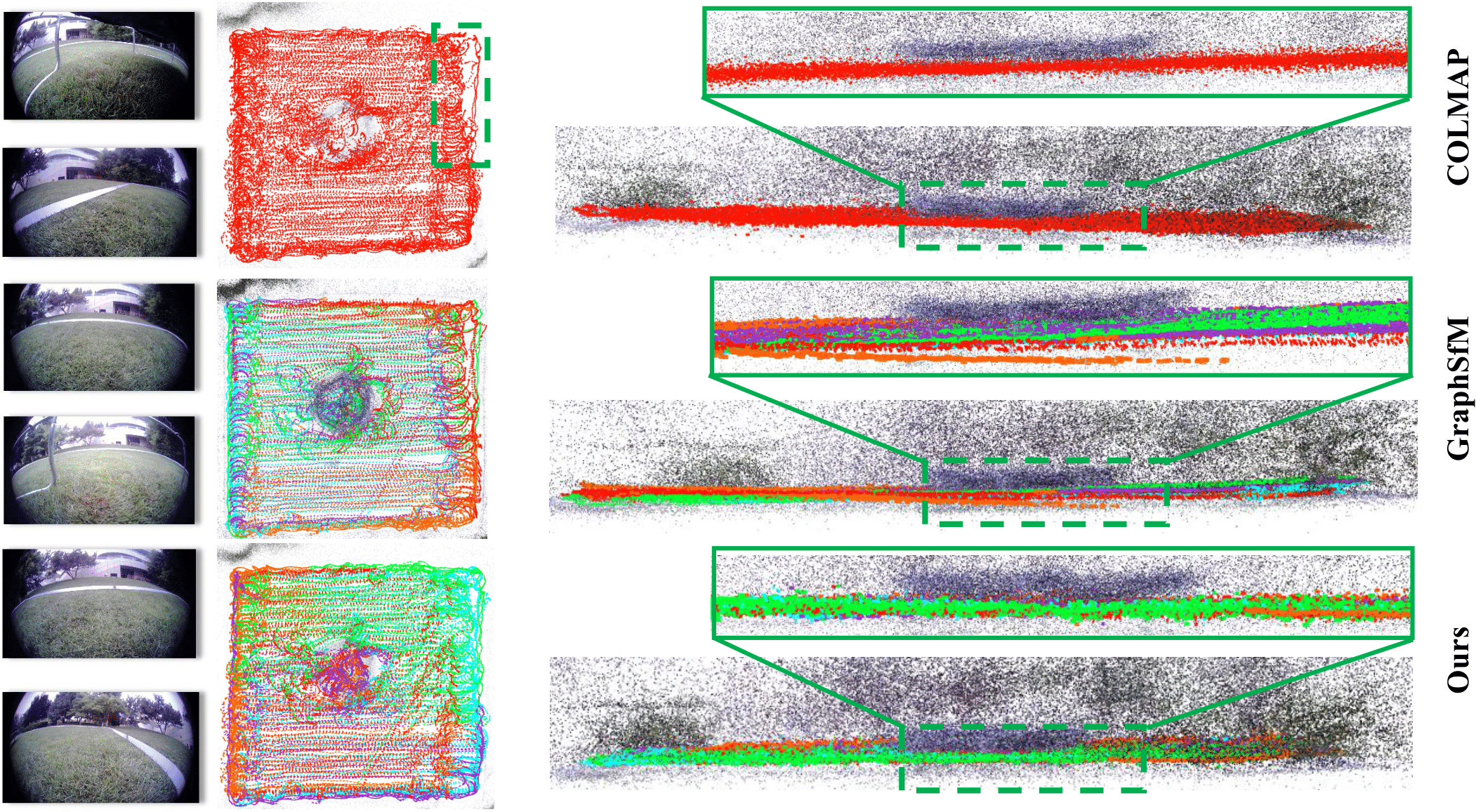
(a) Qualititve comparison on the 711 dataset.

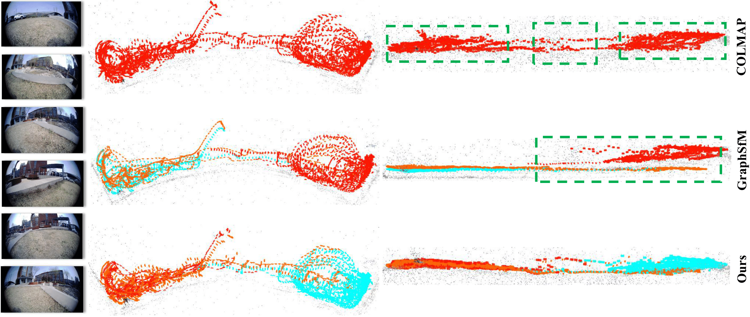
(b) Qualititve comparison on the A4 dataset.

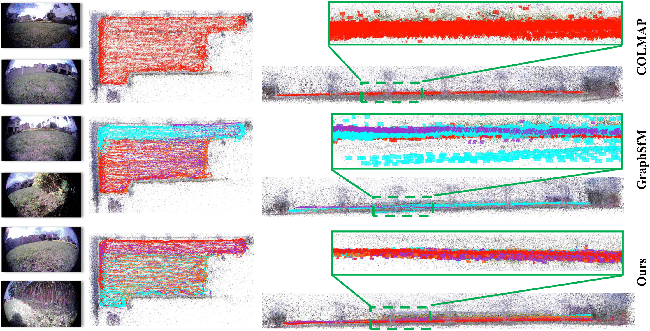
(c) Qualititve comparison on the high free dataset.

Figure 8: Reconstruction comparisons on our self-collected dataset. From left to right are the input images, top-view reconstruction, and side-view reconstruction.

VII-D Ablations of Augmented View Graph

We present more ablation of the augmented view graph on the 4Seasons dataset in Fig. 9. More visualization results on this dataset can be seen in our attached video.

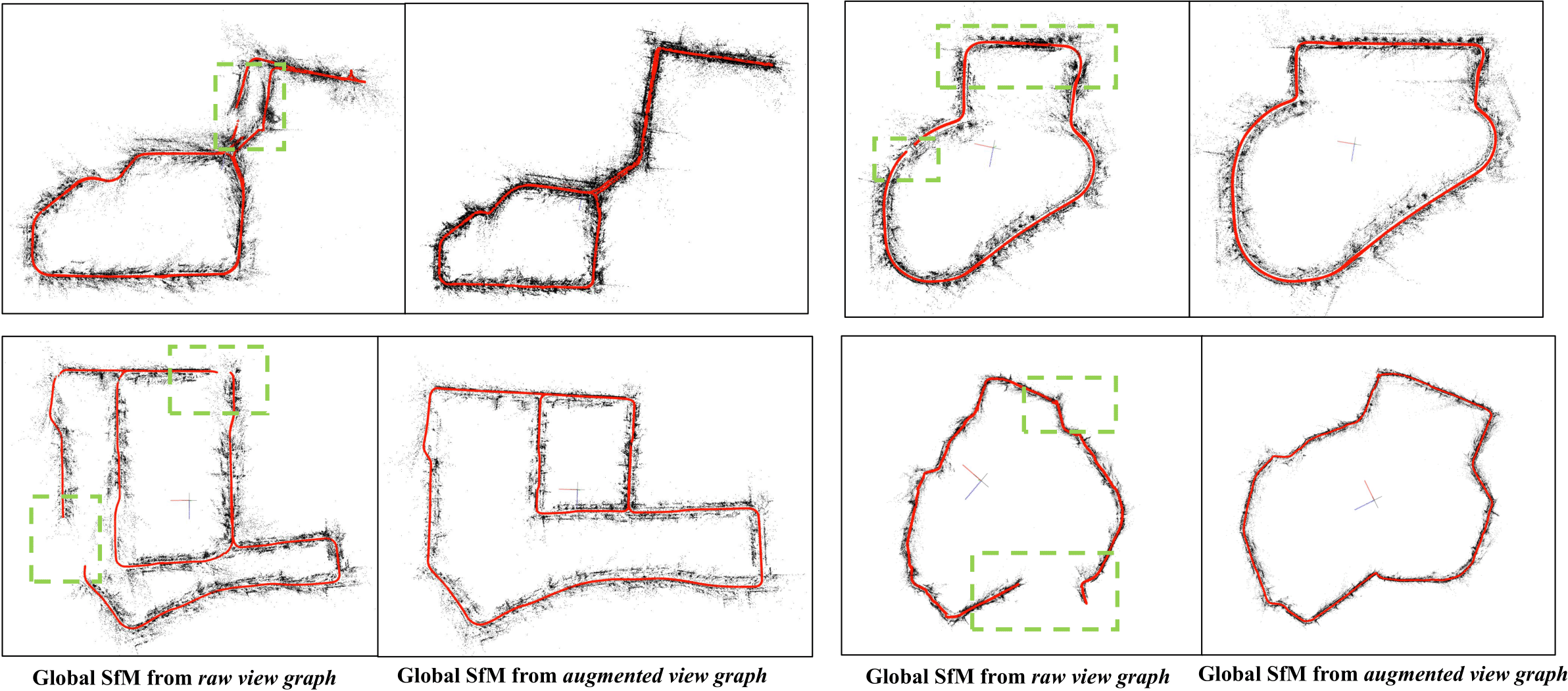
Figure 9: Ablations of our augmented view graph on the 4Seasons dataset.

VII-E Quantitative Results on 4Seasons dataset.

Scene	Sequence	COLMAP [8]					Ours (Global SfM)					Ours (final)
		$N_{c}$	$N_{p}$	$\Delta\mathbf{R}$	$\Delta\mathbf{t}$	$T$	$N_{c}$	$N_{p}$	$\Delta\mathbf{R}$	$\Delta\mathbf{t}$	$T$	$N_{c}$	$N_{p}$	$\Delta\mathbf{R}$	$\Delta\mathbf{t}$	$T$
Neighborhood	recording_2020-10-07_14-53-52	6,326	137,135	0.65	1.78	334.90	6,036	66,777	2.52	1.17	14.68	6,033	109,483	0.74	0.52	123.96
	recording_2020-12-22_11-54-24	6,518	127,892	0.55	3.68	354.35	6,144	64,405	1.10	0.86	15.83	6,144	102,857	0.51	0.62	151.88
	recording_2020-03-26_13-32-55	7,414	148,848	0.61	1.24	603.13	5,982	70,066	0.92	0.79	17.10	5,982	111,807	1.11	0.98	157.76
	recording_2020-10-07_14-47-51	6,688	152,307	0.56	1.67	359.03	6,248	76,305	2.20	1.17	15.70	6,248	121,657	0.75	0.74	152.85
	recording_2021-02-25_13-25-15	6,174	138,807	0.75	1.05	325.65	5,238	62,879	1.00	1.14	15.12	5,238	106,609	0.46	0.81	202.85
	recording_2021-05-10_18-02-12	7,784	149,528	3.04	9.57	444.85	5,834	61,889	1.49	1.38	12.76	5,834	101,102	0.47	0.59	153.36
	recording_2021-05-10_18-32-32	7,174	141,864	2.77	19.15	416.34	6,046	89,010	1.14	1.03	23.81	6,046	142,430	1.49	1.34	264.75
Business Park	recording_2021-01-07_13-12-23	8,016	109,399	0.72	0.75	643.22	9,010	72,096	1.76	1.60	56.16	9,010	100,057	0.66	0.51	465.34
	recording_2020-10-08_09-30-57	11,520	127,013	0.37	1.57	1284.44	8,278	66,087	1.59	1.51	48.72	8,278	108,000	0.63	0.45	366.81
	recording_2021-02-25_14-16-43	7,414	148,848	0.61	1.24	603.13	5,982	70,066	0.92	0.79	17.10	5,982	111,807	1.11	0.98	157.76
Old Town	recording_2020-10-08_11-53-41	19,332	279,989	-	-	2454	12,910	181,569	2.23	2.81	45.72	12,048	279,127	0.55	0.56	254.71
	recording_2021-01-07_10-49-45	16.420	307,383	8.63	360.51	1496.6	12,728	194,340	2.56	3.14	53.18	12,728	327,348	1.55	1.03	238.82
	recording_2021-02-25_12-34-08	18,950	305,461	-	-	2392.98	12,387	182,940	2.02	3.14	40.97	12,387	302,833	0.63	0.74	683.97
Office Loop	recording_2020-03-24_17-36-22	10,188	209,942	1.17	3.40	822.38	9,522	126,680	2.28	2.38	31.87	9,377	214,285	0.97	0.98	166.54
	recording_2020-03-24_17-45-31	8,582	195,738	0.92	3.04	865.48	9,186	122,713	2.79	2.20	33.91	8,940	205,790	0.84	0.85	209.06
	recording_2020-04-07_10-20-31	10,350	223.649	4.22	42.44	795.68	10,184	138,446	2.53	1.78	39.83	10,184	224,499	1.47	1.14	253.24
	recording_2020-06-12_10-10-57	9,990	236,593	18.97	83.94	705.93	10,150	164,062	1.92	1.61	37.32	10,150	246,516	0.76	0.87	206.48
	recording_2021-01-07_12-04-03	9,164	475,950	0.71	2.58	1000.75	10,300	143,715	3.32	2.39	48.68	10,300	223,676	1.08	0.67	249.42
	recording_2021-02-25_13-51-57	9,574	214,695	0.84	2.84	773.32	9,426	122,746	3.80	2.68	28.96	9,426	204,289	1.01	0.91	173.29

TABLE III: Comparison of runtime and accuracy on the 4Seasons datasets. $T$ denotes the runtime (in minutes), $N_{c},N_{p}$ denote the number of registered images and 3D points, respectively, $\Delta\mathbf{R},\Delta\mathbf{t}$ denotes the mean rotation error (in degrees) and translation error (in meters), respectively, and we highlight the best results in bold.

We present the quantitative results on the 4Seasons dataset in Table. III. The 4Seasons dataset provides ground truth camera poses and trajectories from VI-Stereo-DSO [50, 51]. The sensor data contain IMU, GNSS, and stereo images. In our experiment, we do not use the GNSS data. Besides, as this dataset does not provide wheel encode data, we perturb the VI-Stereo-DSO trajectories by Gaussian noise in the x-y-z axes to synthesize wheel encoder data. We strongly recommend readers refer to [15] for more details about the challenged dataset. As is expected, Our method outperforms COLMAP by a large margin in terms of both accuracy and efficiency. In the Old Town scene, COLMAP failed to reconstruct on sequence recording_2020-10-08_11-53-41 and sequence recording_2021-02-25_12-34-08 (we use - to denote the failed cases). As the two sequences contain severe motion blur and tunnels in images, which makes them very challenging to reconstruct. However, our method is also robust to these scenes since it can robustly fuse different sensor data.

References

- [1] P. Sarlin, A. Unagar, M. Larsson, H. Germain, C. Toft, V. Larsson, M. Pollefeys, V. Lepetit, L. Hammarstrand, F. Kahl, and T. Sattler, “Back to the feature: Learning robust camera localization from pixels to pose,” in IEEE Conference on Computer Vision and Pattern Recognition,, 2021, pp. 3247–3257.
- [2] E. Brachmann, M. Humenberger, C. Rother, and T. Sattler, “On the limits of pseudo ground truth in visual camera re-localisation,” in IEEE/CVF International Conference on Computer Vision (ICCV), 2021, pp. 6218–6228.
- [3] M. Dusmanu, O. Miksik, J. L. Schönberger, and M. Pollefeys, “Cross-descriptor visual localization and mapping,” in IEEE/CVF International Conference on Computer Vision (ICCV), 2021, pp. 6058–6067.
- [4] Y. Furukawa and C. Hernández, “Multi-view stereo: A tutorial,” Found. Trends Comput. Graph. Vis., vol. 9, no. 1-2, pp. 1–148, 2015.
- [5] Y. Yao, Z. Luo, S. Li, T. Fang, and L. Quan, “Mvsnet: Depth inference for unstructured multi-view stereo,” in Computer Vision - ECCV 2018 - 15th European Conference, vol. 11212, 2018, pp. 785–801.
- [6] B. Mildenhall, P. P. Srinivasan, M. Tancik, J. T. Barron, R. Ramamoorthi, and R. Ng, “Nerf: Representing scenes as neural radiance fields for view synthesis,” in Computer Vision - ECCV 2020 - 16th European Conference, vol. 12346, 2020, pp. 405–421.
- [7] S. Agarwal, Y. Furukawa, N. Snavely, I. Simon, B. Curless, S. M. Seitz, and R. Szeliski, “Building rome in a day,” Commun. ACM, vol. 54, no. 10, pp. 105–112, 2011.
- [8] J. L. Schönberger and J. Frahm, “Structure-from-motion revisited,” in IEEE Conference on Computer Vision and Pattern Recognition, 2016, pp. 4104–4113.
- [9] P. Moulon, P. Monasse, and R. Marlet, “Global fusion of relative motions for robust, accurate and scalable structure from motion,” in IEEE International Conference on Computer Vision, 2013, pp. 3248–3255.
- [10] Z. Cui and P. Tan, “Global structure-from-motion by similarity averaging,” in IEEE International Conference on Computer Vision, 2015, pp. 864–872.
- [11] C. Sweeney, T. Sattler, T. Höllerer, M. Turk, and M. Pollefeys, “Optimizing the viewing graph for structure-from-motion,” in IEEE International Conference on Computer Vision, 2015, pp. 801–809.
- [12] O. Özyesil and A. Singer, “Robust camera location estimation by convex programming,” in IEEE Conference on Computer Vision and Pattern Recognition, 2015, pp. 2674–2683.
- [13] V. M. Govindu, “Combining two-view constraints for motion estimation,” in IEEE Conference on Computer Vision and Pattern Recognition, 2001, pp. 218–225.
- [14] K. Wilson and N. Snavely, “Robust global translations with 1DSfM,” in European Conference on Computer Vision, vol. 8691, 2014, pp. 61–75.
- [15] P. Wenzel, R. Wang, N. Yang, Q. Cheng, Q. Khan, L. von Stumberg, N. Zeller, and D. Cremers, “4seasons: A cross-season dataset for multi-weather SLAM in autonomous driving,” in Pattern Recognition - 42nd DAGM German Conference, DAGM GCPR 2020, ser. Lecture Notes in Computer Science, vol. 12544. Springer, 2020, pp. 404–417.
- [16] B. Bhowmick, S. Patra, A. Chatterjee, V. M. Govindu, and S. Banerjee, “Divide and conquer: Efficient large-scale structure from motion using graph partitioning,” in Asian Conference on Computer Vision, 2014, pp. 273–287.
- [17] Y. Chen, S. Shen, Y. Chen, and G. Wang, “Graph-based parallel large scale structure from motion,” Pattern Recognition, vol. 107, p. 107537, 2020.
- [18] S. Zhu, T. Shen, L. Zhou, R. Zhang, J. Wang, T. Fang, and L. Quan, “Parallel structure from motion from local increment to global averaging,” arXiv: 1702.08601, 2017.
- [19] S. Zhu, R. Zhang, L. Zhou, T. Shen, T. Fang, P. Tan, and L. Quan, “Very large-scale global SfM by distributed motion averaging,” in IEEE Conference on Computer Vision and Pattern Recognition, 2018, pp. 4568–4577.
- [20] C. Forster, L. Carlone, F. Dellaert, and D. Scaramuzza, “IMU preintegration on manifold for efficient visual-inertial maximum-a-posteriori estimation,” in Robotics: Science and Systems XI,, L. E. Kavraki, D. Hsu, and J. Buchli, Eds., 2015.
- [21] K. Wu, C. X. Guo, G. A. Georgiou, and S. I. Roumeliotis, “VINS on wheels,” in IEEE International Conference on Robotics and Automation,, 2017, pp. 5155–5162.
- [22] R. Hartley and A. Zisserman, Multiple View Geometry in Computer Vision. Cambridge University Press, 2004.
- [23] J. Shi and J. Malik, “Normalized cuts and image segmentation,” IEEE Trans. Pattern Anal. Mach. Intell., vol. 22, no. 8, pp. 888–905, 2000.
- [24] R. J. Lipton, D. J. Rose, and R. E. Tarjan, “Generalized nested dissection,” SIAM Journal on Numerical Analysis, vol. 16, no. 2, pp. 346––358, 1979.
- [25] S. Agarwal, N. Snavely, S. M. Seitz, and R. Szeliski, “Bundle adjustment in the large,” in Computer Vision - ECCV 2010, 11th European Conference on Computer Vision, 2010, pp. 29–42.
- [26] B. Triggs, P. F. McLauchlan, R. I. Hartley, and A. W. Fitzgibbon, “Bundle adjustment - A modern synthesis,” in Vision Algorithms: Theory and Practice, International Workshop on Vision Algorithms, 1999, pp. 298–372.
- [27] C. Wu, “Towards linear-time incremental structure from motion,” in International Conference on 3D Vision, 2013, pp. 127–134.
- [28] H. Cui, S. Shen, X. Gao, and Z. Hu, “Batched incremental structure-from-motion,” in International Conference on 3D Vision, 2017, pp. 205–214.
- [29] V. M. Govindu, “Lie-algebraic averaging for globally consistent motion estimation,” in IEEE Conference on Computer Vision and Pattern Recognition, 2004, pp. 684–691.
- [30] A. Chatterjee and V. M. Govindu, “Efficient and robust large-scale rotation averaging,” in IEEE International Conference on Computer Vision, 2013, pp. 521–528.
- [31] ——, “Robust relative rotation averaging,” IEEE Trans. Pattern Anal. Mach. Intell., vol. 40, no. 4, pp. 958–972, 2018.
- [32] H. P. W and W. R. E, “Robust regression using iteratively reweighted least-squares,” Communications in Statistics-theory and Methods, vol. 9, no. 6, pp. 813–827, 1977.
- [33] K. Wilson, D. Bindel, and N. Snavely, “When is rotations averaging hard?” in Computer Vision - ECCV 2016 - 14th European Conference, vol. 9911, 2016, pp. 255–270.
- [34] T. Goldstein, P. Hand, C. Lee, V. Voroninski, and S. Soatto, “Shapefit and shapekick for robust, scalable structure from motion,” in European Conference on Computer Vision, 2016, pp. 289–304.
- [35] S. P. Boyd, N. Parikh, E. Chu, B. Peleato, and J. Eckstein, “Distributed optimization and statistical learning via the alternating direction method of multipliers,” Foundations and Trends in Machine Learning, vol. 3, no. 1, pp. 1–122, 2011.
- [36] B. Zhuang, L. Cheong, and G. H. Lee, “Baseline desensitizing in translation averaging,” in IEEE Conference on Computer Vision and Pattern Recognition, 2018, pp. 4539–4547.
- [37] H. Cui, X. Gao, S. Shen, and Z. Hu, “Hsfm: Hybrid structure-from-motion,” in IEEE Conference on Computer Vision and Pattern Recognition, 2017, pp. 2393–2402.
- [38] A. Locher, M. Havlena, and L. V. Gool, “Progressive structure from motion,” in Computer Vision - ECCV 2018 - 15th European Conference, 2018, pp. 22–38.
- [39] Z. Jiang, H. Taira, N. Miyashita, and M. Okutomi, “Vio-aided structure from motion under challenging environments,” in 22nd IEEE International Conference on Industrial Technology, 2021, pp. 950–957.
- [40] T. Qin, P. Li, and S. Shen, “Vins-mono: A robust and versatile monocular visual-inertial state estimator,” IEEE Trans. Robotics, vol. 34, no. 4, pp. 1004–1020, 2018.
- [41] R. Mur-Artal, J. M. M. Montiel, and J. D. Tardós, “ORB-SLAM: A versatile and accurate monocular SLAM system,” IEEE Trans. Robotics, vol. 31, no. 5, pp. 1147–1163, 2015.
- [42] Y. Chen, J. Zhao, and L. Kneip, “Hybrid rotation averaging: A fast and robust rotation averaging approach,” in IEEE Conference on Computer Vision and Pattern Recognition, 2021, pp. 10 358–10 367.
- [43] F. Arrigoni, A. Fusiello, E. Ricci, and T. Pajdla, “Viewing graph solvability via cycle consistency,” in IEEE/CVF International Conference on Computer Vision (ICCV), 2021, pp. 5540–5549.
- [44] L. Kneip, D. Scaramuzza, and R. Siegwart, “A novel parametrization of the perspective-three-point problem for a direct computation of absolute camera position and orientation,” in The 24th IEEE Conference on Computer Vision and Pattern Recognition, 2011, pp. 2969–2976.
- [45] R. I. Hartley, J. Trumpf, Y. Dai, and H. Li, “Rotation averaging,” International Journal of Computer Vision, vol. 103, no. 3, pp. 267–305, 2013.
- [46] M. A. Fischler and R. C. Bolles, “Random sample consensus: A paradigm for model fitting with applications to image analysis and automated cartography,” Commun. ACM, vol. 24, no. 6, pp. 381–395, 1981.
- [47] M. Fang, T. Pollok, and C. Qu, “Merge-sfm: Merging partial reconstructions,” in 30th British Machine Vision Conference 2019, 2019, p. 29.
- [48] P. Sarlin, C. Cadena, R. Siegwart, and M. Dymczyk, “From coarse to fine: Robust hierarchical localization at large scale,” in IEEE Conference on Computer Vision and Pattern Recognition, 2019, pp. 12 716–12 725.
- [49] S. Agarwal and K. Mierle, “Ceres solver,” http://ceres-solver.org.
- [50] R. Wang, M. Schwörer, and D. Cremers, “Stereo DSO: large-scale direct sparse visual odometry with stereo cameras,” in IEEE International Conference on Computer Vision. IEEE Computer Society, 2017, pp. 3923–3931.
- [51] L. von Stumberg, V. Usenko, and D. Cremers, “Direct sparse visual-inertial odometry using dynamic marginalization,” in 2018 IEEE International Conference on Robotics and Automation. IEEE, 2018, pp. 2510–2517.
- [52] D. DeTone, T. Malisiewicz, and A. Rabinovich, “Superpoint: Self-supervised interest point detection and description,” in 2018 IEEE Conference on Computer Vision and Pattern Recognition Workshops, 2018, pp. 224–236.
- [53] P. Sarlin, D. DeTone, T. Malisiewicz, and A. Rabinovich, “Superglue: Learning feature matching with graph neural networks,” in 2020 IEEE/CVF Conference on Computer Vision and Pattern Recognition, 2020, pp. 4937–4946.