Optimization of External Stimuli for Populations of Theta Neurons
via Mean-Field Feedback Control*

Abstract

We study a problem of designing “robust” external excitations for control and synchronization of an assembly of homotypic harmonic oscillators representing so-called theta neurons. The model of theta neurons (Theta model) captures, in main, the bursting behavior of spiking cells in the brain of biological beings, enduring periodic oscillations of the electric potential in their membrane.

We study the following optimization problem: to design an external stimulus (control), which steers all neurons of a given population to their desired phases (i.e., excites/slows down its spiking activity) with the highest probability.

This task is formulated as an optimal mean-field control problem for the local continuity equation in the space of probability measures. To solve this problem numerically, we propose an indirect deterministic descent method based on an exact representation of the increment (infinite-order variation) of the objective functional. We discuss some aspects of practical realization of the proposed method, and provide results of numerical experiments.

I INTRODUCTION

The phenomenon of synchronization of oscillatory processes arise in many physical and natural systems involving (relatively large) collections of structurally similar interacting objects. This type of behavior — typically manifested in practice by a formation of (desired or pathological) time-periodic patterns — is demonstrated, e.g., by semiconductors in laser physics [1], vibrating processes in mechanics [2], biochemical reactions [3, 4], as well as in cardiac and neural activity [5, 6, 7].

In connection with oscillatory processes, there naturally arise problems of designing artificial signals that can drive open systems towards (or away from) synchronous oscillations and frequency entrainment; important examples are clinical treatment of neurological and cardiac deceases (such as Parkinson’s disease, epilepsy, and cardiac arrhythmias), control of circadian rhythms [8], organization/destruction of patterns in complex dynamic structures [9], and in neurocomputing [10, 11].

Starting from the pioneer works of Y. Kuramoto and H. Araki, the mathematical imperative in the study of oscillatory ensembles is the mean field dynamics, which describes the behavior of an “averaged” representative of the population instead of tracking all individuals in person. This approach leads to a treatable (and elegant) mathematical representation of the ensemble dynamics even in the case when the cardinality of the population becomes very large, and is naturally translated to the control-theoretical context: in the most of applications, it is technically difficult (or even impossible) to “isolate” the control influence for a particular oscillatory unit; on the contrary, admissible signals usually affect a significant part of the system, or the system as a whole. The topic of control engineering which is focused on designing “simultaneous” control signals for multi-agent systems is familiar under the name ensemble control. “Adaptive” (distributed in the phase space) signals are called mean-field type controls.

In this paper, we address a particular optimal control problem of the type [12] based on a classical oscillatory model [13] from the mathematical neuroscience. Namely, we study the problem of in-phase synchronization of the mean field of so-called theta neurons: to steer a given probability distribution of harmonic phases towards a target one by a simultaneous (ensemble) or individual (mean-field) control.

To solve our problem numerically, we propose a deterministic iterative method of sequential “control improvement”, entailed by an an exact formula for the variation of the objective functional. The proposed approach is based on the optimal mean-field control theory (the dynamic optimization in the space of probability measures) and is quite flexible: it admits one to treat arbitrary statistical ensembles, and can be applied to any problem of a “state-linear” structure, far beyond the considered specific model.

II PROBLEM STATEMENT.
MEAN-FIELD CONTROL SETUP

Consider a population of homotypic oscillatory systems represented by the canonical Ermentrout-Kopell model [13, 14]. This model describes the time-evolution of excitable neurons (customary named “theta neurons”) which endure periodic oscillations of their membrane potential. Each theta neuron in the population is characterized by its phase

$$\theta(t)\in\mathbb{S}^{1}\doteq\mathbb{R}/2\pi\mathbb{Z}$$

which satisfies the ODEs

$$\frac{\,\mathrm{d}}{\,\mathrm{d}t}\theta\doteq\dot{\theta}=v_{u}(\theta,\eta)\doteq(1-\cos\theta)+(1+\cos\theta)\left(u+\eta\right).$$

Here, $\eta$ is the baseline current in the neuron membrane, which varies in a given interval $\mathbb{I}\doteq[a,b]$, and $u$ is an external stimulus.

Theta model provides a simple mathematical description of the so-called spiking behavior. By convention, we say that a neuron produces a spike at time $t$ if $\theta(t)=\pi$. If $\eta>0$ (and $u\equiv 0$) the neuron spikes periodically with the frequency $2\sqrt{\eta}$. If $\eta<0$, the neuron is excitable and can produce spikes after a sufficiently intensive stimulus $u$.

In what follows, $\eta$ is viewed as a parameter of the model fluctuation. In the simplest case, this parameter runs through a finite set $\{\eta_{k},\ k=\overline{1,N}\},$ which corresponds to a finite ensemble $\{\theta_{k},\ k=\overline{1,N}\}$ of theta neurons,

$$\dot{\theta}_{k}=v_{u}(\theta_{k},\eta_{k}),\quad k=\overline{1,N}.$$ (1)

In a more general setup to be discussed below, $\eta$ can be drawn from a given probability distribution.

Remark that (1) falls into the well-recognized Watanabe-Strogatz class of phase oscillators driven by complex functions $t\mapsto H_{k}(t)\in\mathbb{C}$,

$$\dot{\theta}_{k}=\omega_{k}+{\rm Im}\big{(}H_{k}(t)\,e^{-i\,\theta_{k}}\big{)},\quad k=\overline{1,N},$$

where $\omega_{k}$ is the natural (intrinsic) frequency of the $k$th oscillator in the population, and $H_{k}$ is the associated input, modulated by a sinusoidal function (sometimes, this model is called “sinusoidally coupled”); in general, both the natural frequencies and the inputs can be effected by an external driving parameter, furthermore, $H_{k}$ can model interactions between oscillators inside the population. Note that model (1) fits the general statement with

$$\omega_{k}=\omega_{k}(u)\doteq u+\eta_{k}+1,$$

$$H_{k}=H_{k}(u)\doteq i(u+\eta_{k}-1),$$

which does not involve interaction terms (formally, equations (1) are paired only by the common term $u$). In the context of applications, this non-interacting model can be viewed as a “first-order approximation” of a sufficiently sparsely connected neural network (such are real biological ones), especially, if the neurons’ activity is studied over relatively short time periods. The case of interacting neurons will be briefly discussed in section V.

II-A Mean-Field Limit

We are interested in the behavior of system (1) for the case when $N\to\infty$. Introduce extra, “fictitious” states $t\mapsto\eta_{k}(t)$ as solutions to

$$\dot{\eta}_{k}=0,$$ (2)

accompanying (1), and consider the empirical probability measure

$$\mu_{t}^{N}=\frac{1}{N}\sum_{k=1}^{N}\delta_{(\theta_{k}(t),\eta_{k}(t))},$$ (3)

($\delta_{x}$ stands for the Dirac probability measure concentrated at at a point $x$).

The measure-valued function $t\mapsto\mu_{t}^{N}$ designates the statistical behavior of the ensemble $\{(\theta_{k},\eta_{k}),\ k=\overline{1,N}\}$: for any Borel set $A\subset\mathbb{S}^{1}\times\mathbb{I}$, the value $\mu^{N}_{t}(A)$ shows the number of neurons whose phase belongs to $A$.

It is well-known that the curve $t\mapsto\mu_{t}^{N}$ satisfies, in the weak sense, the local continuity equation [15]

$$\partial_{t}\mu_{t}(\theta,\eta)+\partial_{\theta}\big{(}v_{u}(\theta,\eta)\,\mu_{t}(\theta,\eta)\big{)}=0.$$ (4)

Recall that the map $t\mapsto\mu_{t}$ is said to be a weak (distributional) solution of (4) iff

$$\begin{array}[]{c}0=\displaystyle\int_{0}^{T}\,\mathrm{d}t\int_{\mathbb{S}^{1}\times\mathbb{I}}\big{(}\partial_{t}\varphi+\nabla_{x}\varphi\cdot v_{u}\big{)}\,\mathrm{d}\mu_{t}\\[11.38092pt] \forall\,\varphi\in C^{1}_{c}((0,T)\times\mathbb{S}^{1}\times\mathbb{I}).\end{array}$$

($C^{1}_{c}((0,T)\times\mathbb{S}^{1}\times\mathbb{I})$ denotes the space of continuously differentiable functions $(0,T)\times\mathbb{S}^{1}\times\mathbb{I}\mapsto\mathbb{R}$ with compact support in $(0,T)\times\mathbb{S}^{1}\times\mathbb{I}$.) Under standard regularity assumptions, the weak solution exists, it is unique, and it is absolutely continuous as a function $[0,T]\mapsto\mathcal{P}(\mathbb{S}^{1}\times\mathbb{I})$; here $\mathcal{P}(\mathbb{S}^{1}\times\mathbb{I})$ denotes the space of probability measures on $\mathbb{S}^{1}\times\mathbb{I}$ endowed with any Wasserstein distance $W_{p}$, $p\geq 1$ [15].

Equation (4) provides the macroscopic description of the population of microscopic dynamical units (1) called the mean field. This representation remains valid in the limit $N\to\infty$, when $\mu^{N}$ converges to some $\mu\in\mathcal{P}(\mathbb{S}^{1}\times\mathbb{I})$ in $C([0,T];\mathcal{P}(\mathbb{S}^{1}\times\mathbb{I}))$. Moreover, (4) makes sense if phases $\theta$ and currents $\eta$ are drawn from an abstract probability distribution on the cylinder $\mathbb{S}^{1}\times\mathbb{I}$,

$$\mu_{0}=\vartheta\in\mathcal{P}(\mathbb{S}^{1}\times\mathbb{I}).$$ (5)

Indeed, one can immerse the system of ODEs (1) in a deterministic $(\mathbb{S}^{1}\times\mathbb{I})$-valued random process

$$(t,\omega)\mapsto\Theta_{t}(\omega),$$

defined on a probability space $(\Omega,\mathcal{F},\mathbb{P})$ of an arbitrary nature ($\Omega$ is an abstract set, $\mathcal{F}$ is a sigma-algebra on $\Omega$, and $\mathbb{P}$ is a probability measure $\mathcal{F}\mapsto[0,1]$), and satisfying the ODE

$$\frac{\,\mathrm{d}}{\,\mathrm{d}t}\Theta_{t}(\omega)=\left(\begin{array}[]{c}v_{u}\big{(}\Theta_{t}(\omega)\big{)}\\[5.69046pt] 0\end{array}\right).$$

It is a simple technical exercise to check that the function

$$t\mapsto\mu_{t}\doteq(\Theta_{t})_{\sharp}\mathbb{P}$$

solves the Cauchy problem (4), (5) with $\vartheta\doteq(\Theta_{0})_{\sharp}\mathbb{P}$, where the symbol $\sharp$ denotes the operation of pushforward of a measure by a (Borel) function $\Omega\mapsto\mathbb{S}^{1}\times\mathbb{I}$. Note that empirical ensembles (3) fit this setup if $\Omega=\{1,\ldots,N\}$ and $\mathbb{P}$ is the normalized counting measure.

Finally, observe that the variable $\eta$ enters PDE (4) as a parameter rather than state variable. This means that (4) can be regarded as an $\eta$-parametric family of continuity equations on the 1D space $\mathbb{S}^{1}$ rather than a PDE on the 2D space $\mathbb{S}^{1}\times\mathbb{I}$. This observation is essential for the numerical treatment of the problem (4) (see section IV).

II-B Control Signals

Now, we shall fix the class of admissible control signal $u$. Consider two options:

• $u=u(t)$, i.e., the control effects all neurons of the ensemble in the same way. We call this type of external influences the ensemble (simultaneous, common) control. Such a control is statistical in its spirit as it influences the whole ensemble “in average”. As a natural space of such controls we choose

  $$u\in\mathcal{U}\doteq L_{2}([0,T];\mathbb{R}).$$ (6)

• $u=w_{t}(\theta,\eta)$, i.e., the stimulus is adopted to the neuron’s individual characteristics and phase-dependent. The use of such a distributed, mean-field type control

  $$w\in{\mathcal{W}}\doteq L_{2}([0,T];C(\mathbb{S}^{1}\times\mathbb{I};\mathbb{R})),$$ (7)

  assumes some technical option to variate control signals over the spatial domain.

It is natural to expect that the second-type control should perform better. However, let us stress again that the practical implementation of “personalized” control signals is hardly realistic as soon as the number of driven objects is large enough (for experiments that pretend to mimic the biological neural tissue, this number should be astronomic!). In reality, a meaningful class of control signals is $\mathcal{U}$, or something “in the middle” between the mentioned two options.

II-C Performance Criterion

We study a generalization of the optimization problem [12]: to steer the neural population to a target phase distribution at a prescribed (finite) time moment $T>0$ with care about the total energy of the control action. Assuming that the target distribution is given by a (bounded continuous) function $\eta\mapsto\check{\theta}(\eta)$, our optimization problem reads:

$$(P_{1})\qquad\left\{\begin{array}[]{c}\min I[u]=\displaystyle\int F\big{(}\theta,\check{\theta}(\eta)\big{)}\,\mathrm{d}\mu_{T}(\theta,\eta)\\[8.5359pt] \ \ \qquad\displaystyle+\frac{\alpha}{2}\int_{0}^{T}u^{2}(t)\,\mathrm{d}t,\quad\alpha>0,\\[14.22636pt] \displaystyle\mbox{subject to \eqref{PDE}, \eqref{u}},\end{array}\right.$$

where

$$F(\theta,\omega)= \,\frac{1}{2}(\sin\theta-\sin\omega)^{2}+\frac{1}{2}(\cos\theta-\cos\omega)^{2}$$

$$= 1-\cos(\theta-\omega),$$

and

$$\int\doteq\int_{\mathbb{S}^{1}\times\mathbb{I}}.$$

In this problem, the part of state variable is played by the probability measure $\mu_{t}$.

Note that the functional $I$ and the dynamics (4) are linear in $\mu$ (despite the non-linearity of the map $(\theta,\eta)\mapsto v_{u}(\theta,\eta)$). At the same time, (4) contains a product of $\mu$ and $u$, which means that $(P_{1})$ is, in fact, a bi-linear (non-convex) problem.

Standard arguments from the theory of transport equations in the Wasserstein space [15] together with the classical Weierstrass theorem ensure that problem $(P_{1})$ is well posed, i.e., it does have a minimizer within the admissible class $\mathcal{U}$ of control signals (refer, e.g., to [16]).

An alternative version of problem $(P_{1})$ is formulated in terms of the mean-field type control:

$$(P_{2})\quad\left\{\begin{array}[]{c}\min J[w]=\displaystyle\int F\big{(}\theta,\check{\theta}(\eta)\big{)}\,\mathrm{d}\mu_{T}\\[8.5359pt] \qquad\qquad+\displaystyle\frac{\alpha}{2}\int_{0}^{T}\!\!\!\,\mathrm{d}t\int w_{t}^{2}\,\mathrm{d}\mu_{t},\\[14.22636pt] \displaystyle\mbox{subject to \eqref{PDE}, \eqref{w}}.\end{array}\right.$$

In what follows, we shall focus on the “more realistic” statement $(P_{1})$, though all the forthcoming results can be extended, at least formally, to problem $(P_{2})$.

III COST INCREMENT FORMULA.
NUMERICAL ALGORITHM

As it was remarked above, problem $(P_{1})$ is linear in state-measure. This fact allows us to represent the variation of the cost functional $I$ with respect to any variation of control $u$ exactly (without any residual terms). The announced representation follows from the duality with the co-state from Pontryagin’s maximum principle [17], and generalizes the classical exact increment formula for conventional state-linear optimal control problems [18].

Consider two arbitrary controls

$$\bar{u},u\in\mathcal{U},\quad u\neq\bar{u},$$

and let

$$t\mapsto\bar{\mu}_{t}\doteq\mu_{t}[\bar{u}]\mbox{ and }t\mapsto\mu_{t}\doteq\mu_{t}[u]$$

be the respective weak solutions to the continuity equation (4). Let also

$$\bar{p}\doteq p[\bar{u}]:\ (t,\theta,\eta)\mapsto\bar{p}_{t}(\theta,\eta)$$

be a classical solution to the following (non-conservative transport) equation:

$$\partial_{t}p_{t}(\theta,\eta)+ \ \partial_{\theta}p_{t}(\theta,\eta)\cdot v_{\bar{u}(t)}(\theta,\eta)=0.$$ (8)

PDE (8) is known to be dual to the (conservative transport equation) (4); the duality is formally established by the observation that the map

$$t\mapsto\displaystyle\int\bar{p}_{t}\,\mathrm{d}\bar{\mu}_{t}$$

is constant on $[0,T]$. One can check that, under the common regularity of the problem data, this map is an absolutely continuous function $[0,T]\mapsto\mathbb{R}$ (refer to [15] for further details).

As soon as $\bar{p}$ is chosen as a solution to (8) with the terminal condition

$$p_{T}(\theta,\eta)= -F\big{(}\theta,\check{\theta}(\eta)\big{)},$$ (9)

the discussed duality makes it possible to represent the increment (variation)

$$\Delta I\doteq I[u]-I[\bar{u}]$$

of the functional $I$ as follows:

$$-\Delta I=\int_{0}^{T}\big{(}H\left(\mu_{t},\partial_{\theta}\bar{p}_{t},u(t)\right)-H\left(\mu_{t},\partial_{\theta}\bar{p}_{t},\bar{u}(t)\right)\big{)}\,\mathrm{d}t,$$ (10)

where

$$H(\mu,\zeta,u)\doteq u\int\zeta(\theta,\eta)\cdot(1+\cos\theta)\,\mathrm{d}\mu(\theta,\eta)-\frac{\alpha}{2}u^{2}.$$

The derivation of this formula is dropped, since it is completely similar to [18].

Based on representation (10), we can treat problem $(P_{1})$ in the following iterative way: given a reference control $\bar{u}$, one looks for a new “target” signal $u$ that “improves” the functional value, i.e such that $\Delta I<0$. The best choice of the target control is provided by the maximization of the integrand of (10) in the variable $u$:

$$H\left(\mu_{t},\partial_{\theta}\bar{p}_{t},u\right)\to\max,\quad u\in\mathbb{R}.$$

The unique solution of the latter problem is obtain in the analytic form as

$$u_{t}[\mu]=\frac{1}{\alpha}\int\partial_{\theta}\bar{p}_{t}(\theta,\eta)\,(1+\cos\theta)\,\mathrm{d}\mu(\theta,\eta).$$ (11)

Here, it is worthwhile to mention that the reference dual state $\bar{p}$ enters formula (11) only in the form of the partial derivative

$$\bar{\xi}_{t}(\theta,\eta)\doteq\partial_{\theta}\bar{p}_{t}(\theta,\eta).$$

Differentiating (8) and (9) in $\theta$ one can easily check that $\bar{\xi}$ solves the $\eta$-parametric family of the same continuity equations (4) backward in time, starting from the terminal condition

$$\xi_{T}=-\partial_{\theta}F\big{(}\theta,\check{\theta}(\eta)\big{)}\doteq\sin\left(\check{\theta}(\eta)-\theta\right).$$ (12)

Now, (11) can be reformulated in terms of the variable $\bar{\xi}$:

$$u_{t}[\mu]=\frac{1}{\alpha}\int\bar{\xi}_{t}(\theta,\eta)\,(1+\cos\theta)\,\mathrm{d}\mu(\theta,\eta).$$ (13)

Note that the map $(t,\mu)\mapsto u_{t}[\mu]$ can be used as a feedback control

$$[0,T]\times\mathcal{P}(\mathbb{S}^{1}\times\mathbb{I})\mapsto\mathbb{R}$$

of system (4) in the space of probability measures. Injecting this control into (4), we obtain a nonlocal continuity equation

$$\partial_{t}\mu_{t}+\partial_{\theta}\big{(}v_{u[\mu_{t}]}\,\mu_{t}\big{)}=0,\quad\mu_{0}=\vartheta,$$ (14)

which is well-posed (thanks to the fact that function $(\theta,\eta)\mapsto v_{u}(\theta,\eta)$ is smooth and bounded). Solving the last equation numerically, and substituting its solution $t\mapsto\hat{\mu}_{t}\doteq\hat{\mu}_{t}[\bar{u}]$ into (11), we construct the “improved” signal:

$$u(t)=u_{t}[\hat{\mu}_{t}].$$

This idea gives rise to the following Algorithm 1.

Data: $\bar{u}\in\mathcal{U}$ (initial guess), $\varepsilon>0$ (tolerance)

Result: $\{u^{k}\}_{k\geq 0}\subset\mathcal{U}$ such that $I[u^{k+1}]<I[u^{k}]$

$k\leftarrow 0$;

$u^{0}\leftarrow\bar{u}$;

repeat

       $\mu^{k}\leftarrow\hat{\mu}[u^{k}]$;

       $u^{k+1}\leftarrow u[\mu^{k}]$;

       $k\leftarrow k+1$;

      

until $I[u^{k-1}]-I[u^{k}]<\varepsilon$;

Algorithm 1 Numerical algorithm for optimal ensemble control

By construction, Algorithm 1 generates a sequence $\{u^{k}\}_{k\geq 0}\subset\mathcal{U}$ of controls with the property:

$$I^{k+1}\doteq I[u^{k+1}]<I[u^{k}]\doteq I^{k}.$$

Since the sequence of numbers $(I^{k})_{k\geq 0}$ is bounded from below by $\min(P)$ it converges.

Finally, remark that the same line of arguments can be formally applied to problem $(P_{2})$. The respective mean-field type control takes the form

$$w_{t}(\theta,\eta)=\frac{1}{\alpha}\bar{\xi}_{t}(\theta,\eta)\,(1+\cos\theta).$$

This construction gives rise to an iterative method, similar to Algorithm 1.

IV NUMERICAL RESULTS

Let us discuss several aspects of the numerical implementation of Algorithm 1.

First, note that the method proposed here does not involve any intrinsic parametric optimization: the most of indirect algorithms for optimal control require the dynamic adjustment of some internal computational parameters; such are standard methods based on Pontryagin’s maximum principle [19, 20] that imply the internal such as line search for the specification of the “depth” of the needle-shaped (or weak) control variations.

Each iteration of Algorithm 1 requires numerical solution of two problems: one is the linear problem (4), (12) (integrated backward in time), and one for the nonlocal continuity equation (14) (solved numerically forward in time). Since both (4) and (14) have no terms involving partial derivatives in $\eta$, one can think of $\eta$ as a parameter and solve the corresponding parametric families of one-dimensional continuity equations.

Consider the problem $(P)$ with initial distribution of neurons $\mu_{0}$ given by the density function

$$\rho_{0}(\theta,\eta)=\big{(}2+3\cos(2\theta)-2\sin(2\theta)\big{)}\eta,$$

and with constant target function $\check{\theta}(\eta)\equiv\pi$. In other words, our goal is to bring neurons’ states as close as possible to the segment $0\times\mathbb{I}$ by the time moment $T$ with the aid of sufficiently small controls.

Parameters for the computation:

$$T=6,\quad\mathbb{I}=[0.0,1.0],\quad\alpha=1;$$

we used 512 Fourier harmonics in $\theta$ and grid steps

$$\Delta\eta=0.002,\quad\Delta t=0.002.$$

Equations (4) and (14) are integrated by the standard spectral method [21] using the trigonometric Fourier expansion in $\theta$ for each $\eta$ from the grid. Parameters of the algorithm: $\bar{u}\equiv 0$, $\varepsilon=0.01$.

Figure 1: Control input computed by the Algorithm 1

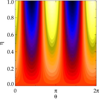
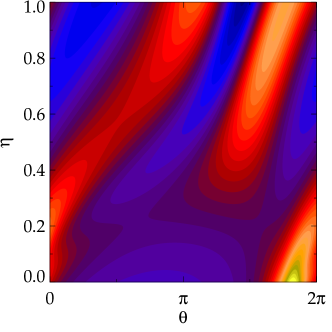
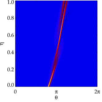
Figure 2: Trajectory $\mu_{t}(\theta,\mu)$ of (4) at time moments $t=0,3$ and 6 (from top to bottom) computed for the optimal control input shown in Fig. 1. The standard “rainbow” color table was used to code the isovalues: from black (minimal values), violet, …, to red (maximal values).

V CONCLUSION

The goal of this paper is to present an approach based on the mean-field control paradigm to solve problems of optimization and synchronization of oscillatory processes (here, the addressed Theta model is among the simplest but prominent examples). The proposed technique can be applied to any state-linear optimal control problem involving (finite or infinite) non-interacting statistical ensembles of an arbitrary nature. In particular, Algorithm 1 can be easily adapted to some other neural model such as SNIPER model, sinusoidal model etc. [12].

We plan to continue this study in the way of natural generalization of model (1) by admitting the interaction between theta neurons,

$$\dot{\theta}_{k}=v_{u}(\theta_{k},\eta_{k})+\frac{1}{N}\sum_{j=1}^{N}K(\theta_{k},\theta_{j}),\quad k=\overline{1,N},$$

where $K$ is certain interaction potential formalizing the spatial connectivity of neurons in the tissue. This will result in control problems of the sort $(P_{1,2})$ stated over the nonlocal continuity equation

$$\partial_{t}\mu_{t}+\partial_{\theta}\big{(}\left[v_{u}+K\star\mu_{t}\right]\,\mu_{t}\big{)}=0$$

involving the term

$$(K\star\mu)(\theta)\doteq\int K(\theta,\zeta)\,\mathrm{d}\mu(\zeta).$$

Such problems are not state-linear anymore, and the exact formula (10) becomes inapplicable. For this case, a promising alternative could be an approach based on Pontryagin’s maximum principle [16].

References

- [1] I. Fischer, Y. Liu, and P. Davis, “Synchronization of chaotic semiconductor laser dynamics on subnanosecond time scales and its potential for chaos communication,” Phys. Rev. A, vol. 62, p. 011801, Jun 2000. [Online]. Available: https://link.aps.org/doi/10.1103/PhysRevA.62.011801
- [2] I. Blekhman, I. Blekhman, and E. Rivin, Synchronization in Science and Technology, ser. ASME press translations. ASME Press, 1988. [Online]. Available: https://books.google.ru/books?id=ao1QAAAAMAAJ
- [3] T. Nishikawa, N. Gulbahce, and A. E. Motter, “Spontaneous reaction silencing in metabolic optimization,” PLOS Computational Biology, vol. 4, no. 12, pp. 1–12, 12 2008. [Online]. Available: https://doi.org/10.1371/journal.pcbi.1000236
- [4] Y. Kuramoto, Chemical Oscillations, Waves, and Turbulence, ser. Dover books on chemistry. Dover Publications, 2003. [Online]. Available: https://books.google.ru/books?id=4ADt7smO5Q8C
- [5] P. J. Uhlhaas and W. Singer, “Neural synchrony in brain disorders: Relevance for cognitive dysfunctions and pathophysiology,” Neuron, vol. 52, no. 1, pp. 155–168, 2006. [Online]. Available: https://www.sciencedirect.com/science/article/pii/S0896627306007276
- [6] S. J. Schiff, K. Jerger, D. H. Duong, T. Chang, M. L. Spano, and W. L. Ditto, “Controlling chaos in the brain,” Nature, vol. 370, no. 6491, pp. 615–620, Aug 1994. [Online]. Available: https://doi.org/10.1038/370615a0
- [7] L. Glass, “Cardiac arrhythmias and circle maps-a classical problem,” Chaos: An Interdisciplinary Journal of Nonlinear Science, vol. 1, no. 1, pp. 13–19, 1991. [Online]. Available: https://doi.org/10.1063/1.165810
- [8] A. Winfree, The Geometry of Biological Time, ser. Interdisciplinary Applied Mathematics. Springer New York, 2013. [Online]. Available: https://books.google.ru/books?id=7qjTBwAAQBAJ
- [9] I. Z. Kiss, C. G. Rusin, H. Kori, and J. L. Hudson, “Engineering complex dynamical structures: Sequential patterns and desynchronization,” Science, vol. 316, no. 5833, pp. 1886–1889, 2007. [Online]. Available: https://www.science.org/doi/abs/10.1126/science.1140858
- [10] F. C. Hoppensteadt and E. M. Izhikevich, “Synchronization of laser oscillators, associative memory, and optical neurocomputing,” Phys. Rev. E, vol. 62, pp. 4010–4013, Sep 2000. [Online]. Available: https://link.aps.org/doi/10.1103/PhysRevE.62.4010
- [11] F. Hoppensteadt and E. Izhikevich, “Synchronization of mems resonators and mechanical neurocomputing,” IEEE Transactions on Circuits and Systems I: Fundamental Theory and Applications, vol. 48, no. 2, pp. 133–138, 2001.
- [12] J.-S. Li, I. Dasanayake, and J. Ruths, “Control and synchronization of neuron ensembles,” IEEE Transactions on Automatic Control, vol. 58, no. 8, pp. 1919–1930, 2013.
- [13] G. B. Ermentrout and N. Kopell, “Parabolic bursting in an excitable system coupled with a slow oscillation,” SIAM Journal on Applied Mathematics, vol. 46, no. 2, pp. 233–253, 1986. [Online]. Available: http://www.jstor.org/stable/2101582
- [14] S. H. Strogatz, Nonlinear dynamics and chaos : with applications to physics, biology, chemistry, and engineering. Second edition. Boulder, CO : Westview Press, a member of the Perseus Books Group, [2015], [2015], includes bibliographical references and index. [Online]. Available: https://search.library.wisc.edu/catalog/9910223127702121
- [15] L. Ambrosio and G. Savaré, “Gradient flows of probability measures,” in Handbook of differential equations: evolutionary equations. Vol. III, ser. Handb. Differ. Equ. Elsevier/North-Holland, Amsterdam, 2007, pp. 1–136.
- [16] N. Pogodaev and M. Staritsyn, “Impulsive control of nonlocal transport equations,” Journal of Differential Equations, vol. 269, no. 4, pp. 3585–3623, 2020. [Online]. Available: https://www.sciencedirect.com/science/article/pii/S002203962030108X
- [17] N. Pogodaev, “Optimal control of continuity equations,” NoDEA Nonlinear Differential Equations Appl., vol. 23, no. 2, pp. Art. 21, 24, 2016.
- [18] M. Staritsyn, N. Pogodaev, R. Chertovskih, and F. L. Pereira, “Feedback maximum principle for ensemble control of local continuity equations: An application to supervised machine learning,” IEEE Control Systems Letters, vol. 6, pp. 1046–1051, 2022.
- [19] A. V. Arguchintsev, V. A. Dykhta, and V. A. Srochko, “Optimal control: Nonlocal conditions, computational methods, and the variational principle of maximum,” Russian Mathematics, vol. 53, no. 1, pp. 1–35, Jan 2009. [Online]. Available: https://doi.org/10.3103/S1066369X09010010
- [20] P. Drag, K. Styczen, M. Kwiatkowska, and A. Szczurek, “A review on the direct and indirect methods for solving optimal control problems with differential-algebraic constraints,” Studies in Computational Intelligence, vol. 610, pp. 91–105, 07 2016.
- [21] J. P. Boyd, Chebyshev and Fourier spectral methods., 2nd ed. Mineola, NY: Dover Publications, 2001.