Topological structures in unconventional scenario for 2D cuprates

Abstract

Numerous experimental data point to cuprates as d-d charge transfer unstable systems whose description implies the inclusion of the three many-electron valence states CuO${}_{4}^{7-,6-,5-}$ (nominally Cu^1+,2+,3+) on an equal footing as a well-defined charge triplet. We introduce a minimal model to describe the charge degree of freedom in cuprates with the on-site Hilbert space reduced to only the three states and make use of the S=1 pseudospin formalism. The formalism constitutes a powerful method to study complex phenomena in interacting quantum systems characterized by the coexistence and competition of various ordered states. Overall, such a framework provides a simple and systematic methodology to predict and discover new kinds of orders. In particular, the pseudospin formalism provides the most effective way to describe different topological structures, in particular, due to a possibility of a geometrical two-vector description of the on-site states. We introduce and analyze effective pseudospin Hamiltonian with on-site and inter-site charge correlations, two types of a correlated one-particle transfer and two-particle, or the composite boson transfer. The latter is of a principal importance for the HTSC perspectives. The 2D S=1 pseudospin system is prone to a creation of different topological structures, which form topologically protected inhomogeneous distributions of the eight local S=1 pseudospin order parameters. We present a short overview of localized topological structures, typical for S=1 (pseudo)spin systems, focusing on unexpected antiphase domain walls in parent cuprates and so-called quadrupole skyrmion, which are believed to be candidates for a topological charge excitation in parent or underdoped cuprates. Puzzlingly, these unconventional structures can be characterized by an uniform distribution of the mean on-site charge, that makes these invisible for X-rays. Quasiclassical approximation and computer simulation are applied to analyze localized topological defects and evolution of the domain structures in ”negative-$U$” model under charge order-superfluid phase transition.

1 Introduction

The origin of high-T_c superconductivity Muller is presently still a matter of great controversy. Both copper and novel non-copper based layered high-T_c materials reveal normal and superconducting state properties very different from that of standard electron-phonon coupled ”conventional”   superconductors.

Copper oxides start out life as insulators in contrast with BCS superconductors being conventional metals. Unconventional behavior of these materials under charge doping, in particular, a remarkable interplay of charge, lattice, orbital, and spin degrees of freedom, strongly differs from that of ordinary metals and merely resembles that of a doped Mott insulator. In addition to the occurrence of unconventional d-wave superconductivity the phase diagram of the high-T_c cuprates does reveal a flurry of various anomalous electronic properties. In normal state, these materials exhibit non-Fermi liquid properties and enter a mysterious pseudogap (PG) regime, characterized by the observation of multiple crossover PG temperatures T^∗’s.

The exotic superconductors differ from ordinary Bardeen-Cooper-Schrieffer (BCS) superconductors in many other points. Thus, muon spin relaxation ($\mu$SR) measurements of the magnetic field penetration depth revealed nearly linear relationship between T_c and the superfluid density in high-T_c cuprates and many other exotic superconductors that cannot be expected in BCS theory, but is typical for Bose-Einstein condensation (BEC) of preformed pairs Uemura . Bosonic scenario for high-T_c cuprates RMP has been elaborated by many authors, in particular, by Alexandrov (see, e.g., Ref. Alexandrov ) who considered real-space bipolarons. It is worth noting that many reasonable predictions of the bipolaronic theory are valid for any local bosons irrespective of its microscopic mechanism. Numerous observations point to the possibility that high-T_c cuprate superconductors may not be conventional BCS or BEC superconductors, but rather manifest a boson-fermion competition in a struggle for the electronic ground state, in particular, a competition between the two- and one-particle transport with resistivity $\propto$T and $\propto$T², respectively.

The most part of the current scenarios, including the Hubbard and $t-J$-models, spin fluctuations, Alexandrov-Mott bipolarons Alexandrov consider cuprates to be homogeneous systems and ignore numerous signatures of the electron and crystalline inhomogeneity Phillips .

Both the normal and high-transition-temperature (high-T_c) superconducting (SC) state in cuprates is believed to be electronically inhomogeneous, in particular, due to a quenched disorder, arising from dopants and/or nonisovalent substitution. However, the dopant-induced impurity potential, seemingly being a natural source of electron inhomogeneity, varies widely among the cuprates that cannot explain observation of an universal, scaling behavior evidencing for an intrinsic electronic tendency toward inhomogeneity in CuO₂ planes. This intrinsic propensity can be stimulated, firstly, by a local out-of-plane nonisovalent substitution, toward formation of in-plane universal inhomogeneity centers. Another stimulating factor of the intrinsic electronic inhomogeneity is related with a two-dimensionality and a competition and intertwinnig of charge, spin and orbital degrees of freedom in CuO₂ planes. Concept of phase separation and percolation phenomena PS ; EmeryKivelson1993 ; EmeryKivelson1995nature ; EmeryKivelson1995prl ; Furrer , stripes Tranquada ; Bianconi ; Zaanen , large polarons Dionne ; GBersuker , nucleation of the mixed valence PJT-(pseudo-Jahn-Teller) phase Moskvin-98 has appeared to be very fruitful for explanation of many puzzling properties of cuprates. Furthermore, some authors Wiegman ; Rodriguez ; Skyrme associate the anomalous properties of cuprates with quasi-2D structure of the active $CuO_{2}$ layers and different topological defects, or vortex-like solitons to be specific collective excitation modes of the 2D vector fields.

The topological order inherent in the doped cuprate endows it with tremendous amount of robustness to various unavoidable ”real-life” material complications Senthil , such as impurities and other coexisting broken symmetries. In general, such a complex, multiscale phase separation does challenge theories of high-temperature superconductivity that include complexity Bianconi2015 .

Recently Moskvin-11 we argued that an unique property of high-T_c cuprates is related with a dual nature of the Mott insulating state of the parent compounds that manifests itself in two distinct energy scales for the charge transfer (CT) reaction: Cu²⁺ + Cu²⁺ $\rightarrow$ Cu¹⁺ + Cu³⁺. Indeed, the $d$ - $d$ CT gap as derived from the optical measurements in parent cuprates such as La₂CuO₄ is 1.5-2.0 eV while the true (thermal) $d$ - $d$ CT gap, or effective correlation parameter $U_{d}$, appears to be as small as 0.4-0.5 eV. It means cuprates should be addressed to be d-d CT unstable systems whose description implies accounting of the three many-electron valence states CuO${}_{4}^{7-,6-,5-}$ (nominally Cu^1+,2+,3+) on an equal footing as a well-defined charge triplet. This allows us to introduce a minimal model for cuprates with the on-site Hilbert space reduced to only three states, three effective valence centers CuO${}_{4}^{7-,6-,5-}$ (Cu^1+,2+,3+) where the electronic and lattice degrees of freedom get strongly locked together, and make use of the S=1 pseudospin formalism Moskvin-11 ; Moskvin-LTP ; Moskvin-09 ; JPCM ; Moskvin-SCES ; Moskvin-JSNM-2016 . Such a formalism constitutes a powerful method to study complex phenomena in interacting quantum systems characterized by the coexistence and competition of various ordered states Batista . Overall, such a framework provides a simple and systematic methodology to predict and discover new kinds of orders. In particular, the pseudospin formalism provides the most effective way to describe different topological structures.

The paper is organized as follows. In Sec. 1 we introduce a working model for the CuO₄ centers based on assumption that the three many-electron valence states CuO${}_{4}^{7-,6-,5-}$ (nominally Cu^1+,2+,3+) form the “on-site” Hilbert space of the CuO₄ plaquettes. We restricted ourselves only by the consideration of the charge degree of freedom and have suggested simple geometrical vector representation for the on-site charge states. In Sec. 2 we have addressed an effectuve pseudospin Hamiltonian for the model cuprate. In Sec. 3 we have considered several simplified versions of the general Hamiltonian. Sec. 4 is devoted to description of unconventional localized topological structures typical for 2D S=1 (pseudo)spin systems. In Sec. 5 we considered localized topological structures in a limiting case of the model, or so-called ”negative-$U$”  model. A brief summary is given in Sec. 6.

2 Working model of the CuO₄ centers

Hereafter we consider the CuO₄ plaquette to be a main element of crystal and electron structure of high-T_c cuprates and introduce a simplified toy model with the “on-site” Hilbert space of the CuO₄ plaquettes reduced to states formed by only three effective valence centers [CuO₄]^7-,6-,5- (nominally Cu^1+,2+,3+, respectively). The centers are characterized by different conventional spin: s=1/2 for Cu²⁺ center and s=0 for Cu^1+,3+ centers, and different orbital symmetry:$B_{1g}$ for the ground states of the Cu²⁺ center, $A_{1g}$ for the Cu¹⁺ centers, and the Zhang-Rice (ZR) $A_{1g}$ or more complicated low-lying non-Zhang-Rice states for the Cu³⁺ center. Electrons of such configurations cannot be treated through a mean-field independent particle approach; therefore, their behavior is studied in terms of auxiliary neither Fermi nor Bose quasiparticles, representing combinations of atomic-like many-electron configurations Ashkenazi .

The key problem that arises from the strong correlations in the normal state of the copper-oxide superconductors is identifying the weakly interacting entities that make a particle interpretation of the current possible. All formulations of superconductivity are reduced to a pairing instability of such well-defined quasiparticles. However, there is good reason to believe that the construction of such entities may not be possible Phillips-2013 .

$$|\Psi\rangle=c_{-1}|Cu^{1+}\rangle+c_{0}|Cu^{2+}\rangle+c_{1}|Cu^{3+}\rangle,$$ (1)

Such an approach immediately implies introduction of the unconventional on-site quantum superpositions that points to many novel effects related with local CuO₄ centers. Validity of such a model implies well isolated ground states of the three centers. This surely holds for the ${}^{1}A_{1g}$ singlet ground state of the Cu¹⁺ centers with nominally filled 3d shell whose excitation energy does usually exceed 2 eV (see, e.g., Ref. Pisarev-2006 and references therein). The $b_{1g}\propto d_{x^{2}-y^{2}}$ character of the ground hole state in CuO${}_{4}^{6-}$ cluster (Cu²⁺ center) seems to be one of a few indisputable points in cuprate physics. A set of low-lying excited states with the energy $\geq$ 1.5 eV includes bonding molecular orbitals with $a_{1g}\propto d_{z^{2}}$, $b_{2g}\propto d_{xy}$, and $e_{g}\propto d_{yz},d_{xz}$ symmetry, as well as purely oxygen nonbonding orbitals with $a_{2g}(\pi)$ and $e_{u}(\pi)$ symmetry (see, e.g., Refs. Moskvin-PRB-02 ; Moskvin-PRL ).

In 1988 Zhang and Rice ZR have proposed that the doped hole in a parent cuprate forms a Cu³⁺ center with a well isolated local spin and orbital ${}^{1}A_{1g}$ singlet ground state which involves a phase coherent combination of the 2p$\sigma$ orbitals of the four nearest neighbor oxygens with the same $b_{1g}$ symmetry as for a bare Cu 3$d_{x^{2}-y^{2}}$ hole. The Zhang-Rice (ZR) singlet is a leading paradigm in modern theories of high-temperature superconductivity. However, both numerous experimental data and the cluster model calculations suggest the involvement of some other physics which introduces low-lying states into the excitation of the doped-hole state, or competition of conventional ZR singlet with another electron removal state(s), in particular, formed by the hole occupation of the oxygen nonbonding $a_{2g}(\pi)$ and $e_{u}(\pi)$ orbitals Moskvin-PRB-02 ; Moskvin-PRL ; NQR-NMR ; Moskvin-FNT-11 ; JETPLett-12 , the $a_{2g}(\pi)$ orbital to be the lowest in energy.

Unified selfconsistent description of the charge, spin, and orbital degrees of freedom for CuO₄ centers with mixed valence is a hardly solvable task so we are forced to address simplified model approaches focusing on the quantum description of the charge degree of freedom that is responsible for superconductivity in cuprates.

2.1 The charge triplet model: S=1 pseudospin formalism

To describe the diagonal and off-diagonal, or quantum local charge order we start with a simplified charge triplet model that implies a full neglect of spin and orbital degrees of freedom Moskvin-SCES . Three charge states of the CuO₄ plaquette: a bare center $M^{0}$=CuO${}_{4}^{6-}$, a hole center $M^{+}$=CuO${}_{4}^{5-}$, and an electron center $M^{-}$=CuO${}_{4}^{7-}$ are assigned to three components of the S=1 pseudospin (isospin) triplet with the pseudospin projections $M_{S}=0,+1,-1$, respectively. Obviously, the model resembles that of so-called semi-hard-core bosons Moskvin-JETP-2015 , which are described by extended Bose-Hubbard model that assumes a truncation of the on-site Hilbert space to the three lowest occupation states n = 0, 1, 2 with further mapping to an anisotropic spin-1 model (see, e.g., Refs.Altman2002 ; Berg2008 ; Berg2010 ). For 2D cuprates these states correspond to a ”electron”  CuO${}_{4}^{7-}$ (Cu¹⁺), ”bare”  CuO${}_{4}^{6-}$ (Cu²⁺), and ”hole”  CuO${}_{4}^{5-}$ (Cu³⁺) centers, respectively.

The S=1 (pseudo)spin algebra includes eight independent nontrivial pseudospin operators, three dipole and five quadrupole operators:

$${\hat{S}}_{z};\;\;{\hat{S}}_{\pm}=\mp\frac{1}{\sqrt{2}}(S_{x}\pm iS_{y});$$ (2)

$${\hat{S}}_{z}^{2};\;\;{\hat{T}}_{\pm}=\{S_{z},S_{\pm}\};\;\;{\hat{S}}^{2}_{\pm}=\frac{1}{2}({\hat{S}}_{x}^{2}-{\hat{S}}_{y}^{2}\pm i\{{\hat{S}}_{x},{\hat{S}}_{y}\}).$$

One should note a principal difference between the s=1/2 and S=1 quantum systems. The only on-site order parameter in the former case is an average spin moment $\langle S_{x,y,z}\rangle$, whereas in the latter one has five additional ”spin-quadrupole”, or spin-nematic order parameters described by traceless symmetric tensors

$$Q_{ij}=\langle\frac{1}{2}\{S_{i},S_{j}\}-\frac{2}{3}\delta_{ij}\rangle.$$ (3)

Interestingly, that in a sense, the $S=\frac{1}{2}$ quantum spin system is closer to a classic one ($S\rightarrow\infty$) with all the order parameters defined by a simple on-site vectorial order parameter $\langle{\bf S}\rangle$ than the S=1 quantum spin system with its eight independent on-site order parameters.

It is worth noting that the three spin-linear (dipole) operators $\hat{S}_{x,y,z}$ and five independent spin-quadrupole operators $Q_{ij}=\frac{1}{2}\{{\hat{S}_{i}},{\hat{S}_{j}}\}-\frac{1}{3}{\hat{\bf S}}^{2}\delta_{ij}$ at S=1 form eight Gell-Mann operators being the generators of the SU(3) group Nadya .

To describe different types of pseudospin ordering in a mixed-valence system we have to introduce eight local (on-site) order parameters: two classical ($diagonal$) order parameters: $\langle S_{z}\rangle$ being a ”valence”, or charge density with an electro-neutrality constraint, and $\langle S_{z}^{2}\rangle$ being the density of polar centers $M^{\pm}$, or ”ionicity”, and six off-diagonal order parameters. The off-diagonal order parameters describe different types of the valence mixing.

It should be emphasized that for the S=1 (pseudo)spin algebra there are two operators: $S_{\pm}$ and $T_{\pm}=\{S_{z},S_{\pm}\}$ that change the pseudo-spin projection by $\pm 1$, with slightly different properties

$$\langle 0|\hat{S}_{\pm}|\mp 1\rangle=\langle\pm 1|\hat{S}_{\pm}|0\rangle=\mp 1,$$ (4)

but

$$\langle 0|\hat{T}_{\pm}|\mp 1\rangle=-\langle\pm 1|(\hat{T}_{\pm}|0\rangle=+1.$$ (5)

It is worth noting the similar behavior of the both operators under the hermitian conjugation: ${\hat{S}}_{\pm}^{\dagger}=-{\hat{S}}_{\mp}$; ${\hat{T}}_{\pm}^{\dagger}=-{\hat{T}}_{\mp}$.

The ${\hat{S}}_{\pm}^{2}$ operator changes the pseudospin projection by $\pm 2$ with the local order parameter

$$\langle S_{\pm}^{2}\rangle = \frac{1}{2}(\langle S_{x}^{2}-S_{y}^{2}\rangle\pm i\langle\{S_{x},S_{y}\}\rangle)={}$$

$${}=c_{+}^{*}c_{-}=c_{x}^{2}-c_{y}^{2}\pm 2ic_{x}c_{y}.$$

Obviously, this on-site off-diagonal order parameter is nonzero only when both $c_{+}$ and $c_{-}$ are nonzero, or for the on-site ”electron-hole”  $M^{-}$(Cu¹⁺)-$M^{+}$(Cu³⁺) superpositions. It is worth noting that the ${\hat{S}}_{+}^{2}$ (${\hat{S}}_{-}^{2}$) operator creates an on-site hole (electron) pair, or composite boson, with a kinematic constraint $({\hat{S}}_{\pm}^{2})^{2}$ = 0, that underlines its ”hard-core”  nature.

Both ${\hat{S}}_{+}$(${\hat{S}}_{-}$) and ${\hat{T}}_{+}$(${\hat{T}}_{-}$) can be associated with the single particle creation (annihilation) operators, however, these are not standard fermionic ones, as well as ${\hat{S}}_{+}^{2}$(${\hat{S}}_{-}^{2}$) operators are not standard bosonic ones. Nevertheless, namely $\langle S_{\pm}^{2}\rangle$ can be addressed as a local superconducting order parameter

The two operators, $S_{\pm}$ and $T_{\pm}$ are related with the two different types of a correlated single-particle transport, these change the pseudospin projection by $\pm 1$. In lieu of these operators one may use two novel operators: ${\hat{P}}_{\pm}=\frac{1}{2}({\hat{S}}_{\pm}+{\hat{T}}_{\pm});\,{\hat{N}}_{\pm}=\frac{1}{2}({\hat{S}}_{\pm}-{\hat{T}}_{\pm})\,,$ which do realize transformations Cu²⁺$\leftrightarrow$Cu³⁺ and Cu¹⁺$\leftrightarrow$Cu²⁺, respectively. In other words, for parent cuprates these are the hole and electron creation operators, respectively. The boson-like pseudospin raising/lowering operators ${\hat{S}}_{\pm}^{2}$ do change the pseudo-spin projection by $\pm 2$ and define a local nematic order parameter

$$\langle S_{\pm}^{2}\rangle=\frac{1}{2}(\langle S_{x}^{2}-S_{y}^{2}\rangle\pm i\langle\{S_{x},S_{y}\}\rangle).$$ (7)

This on-site off-diagonal order parameter with the $d$-type symmetry is nonzero only for the on-site $M^{-}$(Cu¹⁺)-$M^{+}$(Cu³⁺) superpositions. It is worth noting that the ${\hat{S}}_{+}^{2}$ (${\hat{S}}_{-}^{2}$) operator creates an on-site hole (electron) pair, or composite boson, with a kinematic constraint $({\hat{S}}_{\pm}^{2})^{2}$ = 0, that underlines its ”hard-core”  nature. Obviously, the pseudospin nematic average $\langle S_{\pm}^{2}\rangle$ can be addressed to be a local complex superconducting order parameter:

$$\langle S_{\pm}^{2}\rangle=|\langle S_{\pm}^{2}\rangle|e^{\pm i\varphi}.$$ (8)

Both ${\hat{S}}_{+}$(${\hat{S}}_{-}$) and ${\hat{T}}_{+}$(${\hat{T}}_{-}$) can be anyhow related with conventional single particle creation (annihilation) operators, however, these are not standard fermionic ones, as well as ${\hat{S}}_{+}^{2}$(${\hat{S}}_{-}^{2}$) operators are not standard bosonic ones.

It should be noted again that the pseudospin operators are not to be confused with real physical spin operators; they act in a pseudo-space.

2.2 Simple ”geometrical”  representation of the on-site charge states

Making use of a simple classical representation of on-site spin states using arrows is a popular and useful method for describing spin structures through vector fields. However, such an approach works only for classical spins and, under certain limitations, for spin s=1/2. Indeed, for the classical spin all the on-site spin order parameters are derived through $\langle{\bf S}\rangle$, while for s=1/2 $\langle{\bf S}\rangle$ is the only local spin order parameter. At variance with s=1/2 systems for S=1 systems we have additional spin-quadrupole order parameters whose description cannot be realized within framework of a classical ”single-arrow”  representation. Nevertheless, hereafter we propose a novel ”geometrical”  representation that allows us to selfconsistently describe all the on-site S=1 states and make use of the 2D vector fields to describe uniform and nonuniform configurations for model 2D cuprate. In particular, the vector field patterns are of a great importance for physically clear representation of the complex topological structures.

Instead of the three $|1M\rangle$ states one may use the Cartesian basis set ${\bf\Psi}$, or $|x,y,z\rangle$:

$$|10\rangle=|z\rangle\,,\;|1\,{\pm}1\rangle=\mp\frac{1}{\sqrt{2}}(|x\rangle\pm i|y\rangle),$$ (9)

so that the on-site wave function can be written in the matrix form as follows Nadya :

$$\psi=\pmatrix{c_{1}\cr c_{2}\cr c_{3}}=\pmatrix{R_{1}\exp(i\Phi_{1})\cr R_{2}\exp(i\Phi_{2})\cr R_{3}\exp(i\Phi_{3})}\,;\qquad|\vec{R}|^{2}=1\,,$$ (10)

with ${\bf R}=\{\sin\Theta\cos\eta,\sin\Theta\sin\eta,\cos\Theta\}$. Obviously, the minimal number of dynamic variables describing an isolated on-site S=1 (pseudo)spin center equals to four, however, for a more general situation, when the (pseudo)spin system represents only the part of the bigger system, and we are forced to consider the coupling with the additional degrees of freedom, one should consider all the five non-trivial parameters.

The pseudospin matrix has a very simple form within the $|x,y,z\rangle$ basis set:

$$\langle i|\hat{S}_{k}|j\rangle=i\epsilon_{ikj}.$$ (11)

We start by introducing the following set of S=1 coherent states characterized by vectors $\bf a$ and $\bf b$ satisfying the normalization constraint Nadya

$$|{\bf c}\rangle=|{\bf a},{\bf b}\rangle={\bf c}\cdot{\bf\Psi}=({\bf a}+i{\bf b})\cdot{\bf\Psi},$$ (12)

where ${\bf a}$ and ${\bf b}$ are real vectors that are arbitrarily oriented with respect to some fixed coordinate system in the pseudospin space with orthonormal basis ${\bf e}_{1,2,3}$.

The two vectors are related by the normalization condition, so the minimal number of dynamic variables describing the S=1 (pseudo)spin system appears to be equal to four. Hereafter, we would like to emphasize the $director$ nature of the ${\bf c}$ vector field: $|{\bf c}\rangle$ and $|-{\bf c}\rangle$ describe the physically identical states.

It should be noted that in a real space the $|{\bf c}\rangle$ state corresponds to a quantum on-site superposition

$$|{\bf c}\rangle=c_{-1}|Cu^{1+}\rangle+c_{0}|Cu^{2+}\rangle+c_{+1}|Cu^{3+}\rangle\,.$$ (13)

Existence of such unconventional on-site superpositions is a princial point of our model.

Below instead of $\bf a$ and $\bf b$ we will make use of a pair of unit vectors $\bf m$ and $\bf n$, defined as follows Knig :

$$\bf a=\cos\varphi\,{\bf m},\;\bf b=\sin\varphi\,{\bf n}.$$ (14)

For the averages of the principal pseudospin operators we obtain

$$\langle{\bf S}\rangle = \sin 2\varphi\,[{\bf m}\times{\bf n}],$$ (15)

$$\langle\{S_{i},S_{j}\}\rangle = 2(\delta_{ij}-\cos^{2}\varphi\,m_{i}m_{j}-\sin^{2}\varphi\,n_{i}n_{j}).$$ (16)

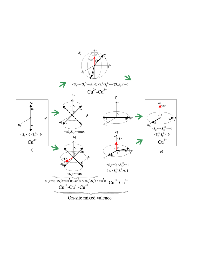
Figure 1: (Color online) Cartoon showing orientations of the ${\bf m}$ and ${\bf n}$ vectors which provide extremal values of different on-site pseudospin order parameters given $\varphi=\pi/4$ (see text for more detail).

Figure 1 shows orientations of the ${\bf m}$ and ${\bf n}$ vectors which provide extremal values of different on-site pseudospin order parameters given $\varphi=\pi/4$. The monovalent Cu²⁺, or $M^{0}$ center, is described by a pair of $\bf m$ and $\bf n$ vectors directed along Z-axis with $|m_{z}|=|n_{z}|$ = 1. We arrive at the Cu²⁺-Cu³⁺ ($M^{0}$-$M^{+}$) or Cu²⁺-Cu¹⁺ ($M^{0}$-$M^{-}$) mixtures if turn $c_{-1}$ or $c_{+1}$, respectively, into zero. The mixtures are described by a pair of $\bf m$ and $\bf n$ vectors whose projections on the XY-plane, ${\bf m}_{\perp}$ and ${\bf n}_{\perp}$, are of the same length and orthogonal to each other: ${\bf m}_{\perp}\cdot{\bf n}_{\perp}$ = 0, $m_{\perp}$ = $n_{\perp}$ with $[{\bf m}_{\perp}\times{\bf n}_{\perp}]$ = $\langle S_{z}\rangle$ = $\pm\sin^{2}\theta$ for $M^{0}$-$M^{\pm}$ mixtures, respectively (see Fig. 1).

It is worth noting that for ”conical”  configurations in Figs. 1b-1d:

$$\langle S_{z}\rangle=0,\;\langle S_{z}^{2}\rangle=\sin^{2}\theta,\;\langle S_{\pm}^{2}\rangle=-\frac{1}{2}\sin^{2}\theta\,e^{\pm 2i\varphi},$$

$$\langle S_{\pm}\rangle=-\frac{i}{\sqrt{2}}\sin 2\theta\,e^{\pm i\varphi},\;\langle T_{\pm}\rangle=0,$$ (17)

(Fig. 1b)

$$\langle S_{z}\rangle=0,\;\langle S_{z}^{2}\rangle=\sin^{2}\theta,\;\langle S_{\pm}^{2}\rangle=-\frac{1}{2}\sin^{2}\theta\,e^{\pm 2i\varphi},$$

$$\langle S_{\pm}\rangle=0,\;\langle T_{\pm}\rangle=\mp\frac{1}{\sqrt{2}}\sin 2\theta\,e^{\pm i\varphi},\;$$ (18)

(Fig. 1c)

$$\langle S_{z}\rangle=-\langle S_{z}^{2}\rangle=-\sin^{2}\theta,\;\langle S_{\pm}^{2}\rangle=0,$$

$$\langle S_{\pm}\rangle=\langle T_{\pm}\rangle=\pm\frac{1}{2}e^{\mp i\frac{\pi}{4}}\sin 2\theta\,e^{\pm i\varphi},$$ (19)

(Fig. 1d). Figures 1e,f do show the orientation of ${\bf m}$ and ${\bf n}$ vectors for the local binary mixture Cu¹⁺-Cu³⁺, and Fig.1g does for monovalent Cu³⁺ center. It is worth noting that for binary mixtures Cu¹⁺-Cu²⁺ and Cu³⁺-Cu²⁺ we arrive at the same algebra of the ${\hat{S}}_{\pm}$ and ${\hat{T}}_{\pm}$ operators with $\langle S_{\pm}\rangle=\langle T_{\pm}\rangle$, while for ternary mixtures Cu¹⁺-Cu²⁺-Cu³⁺ these operators describe different excitations. Interestingly that in all the cases the local Cu²⁺ fraction can be written as follows:

$$\rho(Cu^{2+})=1-\langle S_{z}^{2}\rangle=\cos^{2}\theta.$$ (20)

3 Effective S=1 pseudospin Hamiltonian

Effective S=1 pseudospin Hamiltonian which does commute with the z-component of the total pseudospin $\sum_{i}S_{iz}$ thus conserving the total charge of the system can be written to be a sum of potential and kinetic energies:

$${\hat{H}}={\hat{H}}_{pot}+{\hat{H}}_{kin}\,,$$ (21)

where

$${\hat{H}}_{pot}=\sum_{i}(\Delta_{i}S_{iz}^{2}-\mu S_{iz})+\sum_{i<j}V_{ij}S_{iz}S_{jz},$$ (22)

with a charge density constraint:

$$\frac{1}{2N}\sum_{i}\langle S_{iz}\rangle=\Delta n,$$ (23)

where $\Delta n$ is the deviation from a half-filling ($N_{M^{+}}$ = $N_{M^{-}}$). The first single-site term in ${\hat{H}}_{pot}$ describes the effects of a bare pseudo-spin splitting, or the local energy of $M^{0,\pm}$ centers and relates with the on-site density-density interactions, $\Delta=U/2$, $U$ being the correlation parameter. The second term may be related to a pseudo-magnetic field $\parallel$ $Z$ with $\mu$ being the hole chemical potential. The third term in ${\hat{H}}_{pot}$ describes the inter-site density-density interactions.

In general the Hamiltonian (22) describes so-called atomic limit of the model.

Kinetic energy ${\hat{H}}_{kin}={\hat{H}}_{kin}^{(1)}+{\hat{H}}_{kin}^{(2)}$ is a sum of one-particle and two-particle transfer contributions. In terms of ${\hat{P}}_{\pm}$ and ${\hat{N}}_{\pm}$ operators the Hamiltonian ${\hat{H}}_{kin}^{(1)}$ reads as follows:

$${\hat{H}}_{kin}^{(1)} = \frac{1}{2}\sum_{i\not=j}\big{[}t^{p}_{ij}P_{i+}P_{j-}+t^{n}_{ij}N_{i+}N_{j-}+{}$$ (24)

$${}+\frac{1}{2}t^{pn}_{ij}(P_{i+}N_{j-}+P_{i-}N_{j+})+h.c.\big{]}.$$

All the three terms here suppose a clear physical interpretation. The first $PP$-type term describes one-particle hopping processes: $Cu^{3+}+Cu^{2+}\leftrightarrow Cu^{2+}+Cu^{3+}$, that is a rather conventional motion of the hole $M^{+}$ ($Cu^{3+}$) centers in the lattice formed by $M^{0}$ ($Cu^{2+}$)-centers ($p$-type carriers, respectively) or the motion of the $M^{0}$ ($Cu^{2+}$)-centers in the lattice formed by hole $M^{+}$ ($Cu^{3+}$) centers ($n$-type carriers, respectively). The second $NN$-type term describes one-particle hopping processes: $Cu^{1+}+Cu^{2+}\leftrightarrow Cu^{2+}+Cu^{1+}$, that is a rather conventional motion of the electron $M^{-}$ ($Cu^{1+}$) centers in the lattice formed by $M^{0}$ ($Cu^{2+}$)-centers ($n$-type carriers) or the motion of the $M^{0}$ ($Cu^{2+}$)-centers in the lattice formed by electron $M^{-}$ ($Cu^{1+}$) centers ($p$-type carriers). These hopping processes are typical ones for heavily underdoped or heavily overdoped cuprates. The third $PN$ ($NP$) term in ${\hat{H}}_{kin}^{(1)}$ defines a very different one-particle hopping process: $Cu^{2+}+Cu^{2+}\leftrightarrow Cu^{3+}+Cu^{1+},Cu^{1+}+Cu^{3+}$, that is the local disproportionation/recombination, or the electron-hole pair creation/annihilation. Interestingly, the term can be related with a local pairing as the $Cu^{1+}$ center can be addressed to be an electron pair (= composite electron boson) localized on the $Cu^{3+}$ center or vice versa the $Cu^{3+}$ center can be addressed to be a hole pair (= composite hole boson) localized on the $Cu^{1+}$ center.

Hamiltonian ${\hat{H}}_{kin}^{(2)}$:

$${\hat{H}}_{kin}^{(2)}=\sum_{i<j}t_{ij}^{b}(S_{i+}^{2}S_{j-}^{2}+S_{i-}^{2}S_{j+}^{2})\,,$$ (25)

describes the two-particle (local composite boson) inter-site hopping, that is the motion of the electron (hole) center in the lattice formed by the hole (electron) centers, or the exchange reaction: $Cu^{3+}+Cu^{1+}\leftrightarrow Cu^{1+}+Cu^{3+}$. In other words, $t^{b}_{ij}$ is the transfer integral for the local composite boson that governs the Bose condensation temperature. Its value is believed to be of a particular interest in cuprate physics

The magnitude of the effective transfer integral $t_{B}$ can be written as follows:

$$t_{B}=\langle 20|V_{ee}|02\rangle-\sum_{11}\frac{\langle 20|\hat{h}|11\rangle\langle 11|\hat{h}|02\rangle}{\Delta_{dd}}\,,$$ (26)

where the first term describes a simultaneous tunnel transfer of the electron pair due to Coulomb coupling $V_{ee}$ and may be called as a ”potential”  contribution, while the second describes a two-step (20-11-02) electron-pair transfer via successive one-electron transfer due to the one-electron Hamiltonian, and may be called as ”kinetic”  contribution, $\Delta_{dd}$ is a Franck-Condon $d$-$d$ CT energy. As it is emphasized by P.W. Anderson PWA the value of the seemingly leading kinetic contribution to the composite boson transport is closely related to the respective contribution to the exchange integral, i.e. $t_{B}\approx$ 0.1 eV in cuprates. From the other hand, this parameter determines so-called S-P separation for electron-hole dimers Moskvin-11 and can be reliably estimated from different optical data, both conventional optical conductivity MIR ; Gruninger and unconventional nonlinear optics Kishida ; Ono-04 ; Maeda-04 . For different parent cuprates with corner-sharing CuO₄ plaquettes ( Sr₂CuO₃, Sr₂CuO₂Cl₂, YBa₂Cu₃O₆) the optical data point to surprisingly close values: $t_{B}\approx$ 0.1 eV.

These estimations point to a promising upper limit of $T\approx$ 1000 K for the local bosonic superfluidity in cuprates and leaves a hope for the realization in the cuprates of the room-temperature superconductivity.

Similar to conventional spin systems the S = 1 pseudospin formalism allows us to predict various types of diagonal and off-diagonal long-range order and pseudospin excitations, including commensurate and incommensurate charge orders (pseudospin density waves), superfluid and supersolid phases, different topological excitations typical for 2D systems Moskvin-JETP-2015 . However, at variance with typical spin systems, in particular, in 3d-oxides the pseudospin system appears to be strongly anisotropic one with an enhanced role of frustrative effects of the in-plane next-nearest neighbor couplings, inter-plane coupling, and different non-Heisenberg biquadratic interactions. Despite the difference we can translate many results of the spin S = 1 algebra to our pseudospin system. Turning to a classification of the possible homogeneous phases of the charge states of the model cuprates and its phase diagram we introduce $monovalent$ MV-1 (Cu¹⁺, Cu²⁺, Cu³⁺), $bivalent$ MV-2 (Cu^1+,2+, Cu^2+,3+, Cu^1+,3+), and $trivalent$ MV-3 (Cu^1+,2+,3+) phases in accordance with character of the on-site superpositions (13). Then, in accordance with the above nomenclature of spin phases and the charge triplet – S = 1 pseudospin correspondence we arrive at a parent monovalent (Cu²⁺) phase as an analogue of the quantum paramagnetic (QPM) phase to be a quantum analogue of the ”easy-plane” phase, the $XY^{13}$, $XY^{123}$, $XY$-$Z_{FM}^{13}$, $XY$-$Z_{FM}^{23}$, $XY$-$Z_{FM}^{12}$, $XY$-$Z_{FM}^{123}$, $XY$-$Z_{AFM}^{13}$, $XY$-$Z_{AFM}^{123}$, $XY$-$Z_{FIM}^{13}$, $XY$-$Z_{FIM}^{123}$, $Z_{FM}^{1}$, and $Z_{FM}^{3}$ phases as mono-, bi-, and trivalent analogues of respective spin phases. All the metallic phases with $XY^{13}$ and $XY^{123}$ components do admit in principle the pseudospin nematic order $\langle S_{\pm}^{2}\rangle\not=$ 0 related with the high-T_c superconductivity (HTSC). In all the trivalent phases the superconducting order competes with a spin ordering. Moreover, in $XY$-$Z_{FIM}^{123}$ phase we deal with a competition of superconducting, spin, and charge orders. It is worth noting that the $XY$-$Z$ nomenclature does strictly reflect an interplay of kinetic ($XY$-terms) and potential ($Z$-term) energies, or itineracy and localization.

For undoped model cuprate with $\sum_{i}\langle S_{iz}\rangle$ = 0 (half filling) given rather large positive $\Delta>\Delta_{1}$ we arrive at insulating monovalent quantum paramagnetic $M^{0}$ (Cu²⁺)-phase, a typical one for Mott-Hubbard insulators. In parent cuprates, such as La₂CuO₄, the Cu²⁺ ions form an antiferromagnetically (AF) coupled square lattice of s = 1/2 spins, which could possibly realize the resonant valence bond (RVB) liquid of singlet spin pairs. In the RVB state the large energy gain of the singlet pair state, resonating between the many spatial pairing configurations, drives strong quantum fluctuations strong enough to suppress long range AF order. However, by lowering the $\Delta$ below $\Delta_{1}$ the undoped cuprate can be turned first into metallic and superconducting $XY^{123}$ phase, and given $\Delta<\Delta_{2}$ into a fully disproportionated MV-2 system of electron $M^{-}$ and hole $M^{+}$ centers ($M^{\pm}$-phase) with $\langle S_{iz}^{2}\rangle$ = 1 (Fig. 1), or electron-hole Bose liquid (EHBL) Moskvin-11 ; Moskvin-LTP ; Moskvin-09 ; JPCM ; Moskvin-98 . There is no single particle transport: $\langle S_{\pm}\rangle=\langle T_{\pm}\rangle$ = 0, while the bosonic one may exist, and, in common, $\langle S_{\pm}^{2}\rangle\not=$ 0.

Strictly speaking the S=1 pseudospin Hamiltonian (21) describes an extended bosonic Hubbard model (EBHM) with truncation of the on-site Hilbert space to the three lowest occupation states n = 0, 1, 2, or the model of semi-hard-core bosons Moskvin-JETP-2015 . The EBHM Hamiltonian is a paradigmatic model for the highly topical field of ultracold gases in optical lattices, however, this is one of the working models to describe the insulator-metal transition and high-temperature superconductivity.

The pseudospin Hamiltonian (21) can be generalized for cuprates to include spin and orbital degrees of freedom Moskvin-JSNM-2016 , in particular, to take into account an intra-plaquette charge nematicity. Indeed, different orbital symmetry, $B_{1g}$ and $A_{1g}$ of the ground states for Cu²⁺ and Cu^1+,3+, respectively, unequivocally should result in a spontaneous orbital symmetry breaking accompanying the formation of the on-site superpositions with emergence of the on-site orbital order parameter of the $B_{1g}=B_{1g}\times A_{1g}$ ($\propto d_{x^{2}-y^{2}}$) symmetry. In frames of the CuO₄ cluster model the rhombic $B_{1g}$-type symmetry breaking may be realized both by the $b_{1g}$-$a_{1g}$ ($d_{x^{2}-y^{2}}$-$d_{z^{2}}$) mixing for central Cu ion or through the oxygen subsystem either by emergence of different charge densities on the oxygens placed symmetrically relative to the central Cu ion and/or by the $B_{1g}$-type distortion of the CuO₄ plaquette resulting in different Cu-O separations for these oxygens. The latter effect seems to be natural for Cu¹⁺ admixtures. Indeed, at variance with Cu²⁺ and Cu³⁺ ions the Cu¹⁺ ion due to a large intra-atomic $s$ - $d$ - hybridization does prefer a dumbbell O-Cu-O linear configuration thus making large rhombic distortions of the CuO₄ cluster. Taking into account two energetically equivalent $B_{1g}$-type charge imbalance/distortions of the isolated CuO₄ plaquette in both cases we can introduce a dichotomic nematic variable that can be build in into effective pseudospin Hamiltonian. The STM nematic and ¹⁷O NQR Haase measurements of a static nematic order in cuprates support a charge imbalance between the density of holes at the oxygen sites oriented along $a$- and $b$-axes, however, there are clear signatures of the $B_{1g}$-type distortion (half-breathing mode) instabilities even in hole-doped superconducting cuprates which can be addressed to be a true ”smoking gun” for electronic Cu¹⁺ centers. The two dynamically coexisting sets of CuO₄ clusters with different in-plane Cu-O interatomic distances have been really found by polarized Cu K-edge EXAFS in La_1.85Sr_0.15CuO₄ Bianconi . Giant phonon softening and line broadening of electronic origin of the longitudinal Cu-O bond stretching phonons near half-way to the zone boundary was observed in hole-doped cuprates (see, e.g., Ref. phonon and references therein). Their amplitude follows the superconducting dome that supports our message about a specific role of electron-hole Cu¹⁺-Cu³⁺ pairs in high-T_c superconductivity.

Conventional spin s=1/2 degree of freedom can be build in our effective Hamiltonian, if we transform conventional Heisenberg spin exchange Cu²⁺-Cu²⁺ coupling as follows

$${\hat{H}}_{ex}=\sum_{i<j}{\hat{I}}_{ij}(\hat{\bf s}_{i}\cdot\hat{\bf s}_{j}),$$ (27)

where

$${\hat{I}}_{ij}=(1-{\hat{S}}_{iz}^{2})I_{ij}(1-{\hat{S}}_{jz}^{2})$$ (28)

is an effective exchange integral, $(1-{\hat{S}}_{iz}^{2})$ is a projection operator which picks out the s=1/2 Cu²⁺ center, $I_{ij}$ is the conventional Cu²⁺-Cu²⁺ exchange integral. It is worth noting that $(1-\langle{\hat{S}}_{iz}^{2}\rangle)$ can be addressed to be a Cu²⁺ spin density. Obviously, the spin exchange provides an energy gain to the parent antiferromagnetic insulating (AFMI) phase with $\langle{\hat{S}}_{iz}^{2}\rangle$ = 0, while local superconducting order parameter is maximal given $\langle{\hat{S}}_{iz}^{2}\rangle$ = 1. In other words, the superconductivity and magnetism are nonsymbiotic phenomena with competing order parameters giving rise to an intertwinning, glassiness, and other forms of electronic heterogeneities, especially considering the same order of magnitude for $I_{ij}$ and $t^{B}_{ij}$. Simplified spin-pseudospin model describing a spin-charge competition in atomic limit with an unconventional spin-charge phase separation in cuprates has been studied by us recently spin-charge .

4 Typical simplified S=1 spin and pseudospin models

Despite many simplifications, the effective pseudospin Hamiltonian (21) is rather complex, and represents one of the most general forms of the anisotropic S=1 non-Heisenberg Hamiltonian. Its real spin counterpart corresponds to an anisotropic S=1 magnet with a single-ion (on-site) and two-ion (inter-site bilinear and biquadratic) symmetric anisotropy in an external magnetic field under conservation of the total $S_{z}$. Spin Hamiltonian (21) describes an interplay of the Zeeman, single-ion and two-ion anisotropic terms giving rise to a competition of an (anti)ferromagnetic order along Z-axis with an in-plane $XY$ magnetic order. Simplified versions of anisotropic S=1 Heisenberg Hamiltonian with bilinear exchange have been investigated rather extensively in recent years. Their analysis seems to provide an instructive introduction to description of our generalized pseudospin model.

4.1 Anisotropic S = 1 Heisenberg model with a single-ion anisotropy

Typical S = 1 spin Hamiltonian with uniaxial single-site and exchange anisotropies reads as follows:

Effective pseudospin Hamiltonian (21) can be reduced to a typical S = 1 spin Hamiltonian with uniaxial single-ion and bilinear exchange anisotropies:

$${\hat{H}} = \sum_{i<j}J_{ij}(S_{ix}S_{jx}+S_{iy}S_{jy}+\lambda S_{iz}S_{jz})+{}$$ (29)

$${}+\sum_{i}DS_{iz}^{2}-\sum_{i}hS_{iz},$$

if we neglect the two-particle transport term (25) and restrict ourselves by bilinear terms in the single-particle transport. Correspondence with our pseudospin Hamiltonian points to $D=\Delta$, $J_{ij}=t_{ij}$, $\lambda J_{ij}=V_{ij}$. Usually one considers the antiferromagnet with $J>0$ since, in general, this is the case of more interest. However, the Hamiltonian (29) is invariant under the transformation $J,\lambda\rightarrow-J,-\lambda$ and a shift of the Brillouin zone ${\bf k}\rightarrow{\bf k}+(\pi,\pi)$ for 2D square lattice. The system described by the Hamiltonian (29) can be characterized by local (on-site) spin-linear order parameters $\langle{\bf S}\rangle$ and spin-quadratic (quadrupole spin-nematic) order parameters $Q^{2}_{0}=Q_{zz}=\langle S_{z}^{2}-\frac{2}{3}\rangle$ and $Q^{2}_{\pm 2}=\langle S_{\pm 1}^{2}\rangle$.

The model has been studied rather extensively in recent years by several methods, e.g., molecular field approximation, spin-wave theories, exact numerical diagonalizations, nonlinear sigma model, quantum Monte Carlo, series expansions, variational methods, coupled cluster approach, self-consistent harmonic approximation, and generalized SU(3) Schwinger boson representation (see, e.g., Refs. Sengupta2007 ; Hamer2010 ; Lapa2013 and references therein).

The spectrum of the spin Hamiltonian (29) in the absence of external magnetic field changes drastically as $\Delta$ varies from very small to very large positive or negative values. A strong ”easy-plane”  anisotropy for large positive $\Delta>0$ favors a singlet phase where all the spins are in the $S_{z}=0$ ground state. This quadrupole ($Q_{zz}$ = -$\frac{2}{3}$) phase has no magnetic order, and is aptly referred to as a quantum paramagnetic phase (QPM), which is separated from the ”ordered”  state by a quantum critical point (QCP) at some $\Delta$ = $\Delta_{1}$. A strong ”easy-axis”  anisotropy for large negative $\Delta\leq\Delta_{2}$, favors a spin ordering along $Z$, the ”easy axis”, with the on-site $S_{z}=\pm 1$ ($Z$-phase). The order parameter will be ”Ising-like”  and long-range (staggered) diagonal order will persist at finite temperature, up to a critical line T${}_{c}(\Delta)$. For intermediate values $\Delta_{1}>\Delta>\Delta_{2}$ the Hamiltonian will have O(2) symmetry and the system is in a gapless $XY$ phase. At $T=0$ the O(2) symmetry will be spontaneously broken and the system will exhibit spin order in some direction. Although there will be no ordered phase at finite temperature one expects a finite temperature Kosterlitz-Thouless transition. At finite effective field $h_{z}$ but $\lambda$ = 1 the $XY$ phase transforms into a canted antiferromagnetic $XY$-$Z_{FM}$ phase, the spins acquire a uniform longitudinal component which increases with field and saturates at the fully polarized (FP) state (all $S_{z}$ = 1, $Z_{FM}$ phase) above the saturation field $h_{s}$. However, at $D>$ 0 and $\lambda>$ 1 the phase diagram contains an extended spin supersolid or conical phase $XY$-$Z_{FIM}$ with ferrimagnetic $z$-order that does exist over a range of magnetic fields Sengupta2007 ; Hamer2010 ; Lapa2013 .

4.2 ”Negative”-$U$ model and its relevance for 2D cuprates

At large negative values of the on-site correlation parameter $\Delta$ = $U$/2 we arrive at the ground state of our model cuprate to be a system of electron CuO${}_{4}^{7-}$ and hole CuO${}_{4}^{5-}$ centers coupled by inter-site correlations and two-particle transport, while single-particle transport described by ${\hat{H}}_{kin}^{(1)}$ is suppressed due to large value of the transfer energy. This electron-hole liquid is equivalent to the lattice hard-core ($hc$) Bose system with an inter-site repulsion and can be termed as electron-hole Bose liquid (EHBL). Indeed, one may address the electron $M^{-}$ center to be a system of a local composite boson ($e^{2}$) localized on the hole $M^{+}$ center: $M^{-}=M^{+}+e^{2}$. For such a system, the pseudo-spin Hamiltonian (21) can be mapped onto the Hamiltonian of $hc$ Bose gas on a lattice (see Refs. RMP ; bubble ; bubble-2 and references therein)

$$H_{hc} = -\sum\limits_{\langle ij\rangle}t_{ij}{\hat{P}}({\hat{b}}_{i}^{\dagger}{\hat{b}}_{j}+{\hat{b}}_{j}^{\dagger}{\hat{b}}_{i}){\hat{P}}+{}$$ (30)

$${}+\sum\limits_{\langle ij\rangle}V_{ij}n_{i}n_{j}-\mu\sum\limits_{i}n_{i},$$

where ${\hat{P}}$ is the projection operator which removes double occupancy of any site, ${\hat{b}}^{\dagger}({\hat{b}})$ are the Pauli creation (annihilation) operators which are Bose-like commuting for different sites $[{\hat{b}}_{i},{\hat{b}}_{j}^{\dagger}]=0,$ if $i\neq j,$ $[{\hat{b}}_{i},{\hat{b}}_{i}^{\dagger}]=1-2n_{i}$, $n_{i}={\hat{b}}_{i}^{\dagger}{\hat{b}}_{i}$; $N$ is a full number of sites, $\mu$ the chemical potential determined from the condition of fixed full number of bosons $\sum_{i}\langle n_{i}\rangle$ or concentration $n=\frac{1}{N}\sum_{i}\langle n_{i}\rangle\in[0,1]$. The $t_{ij}$ denotes an effective transfer integral, $V_{ij}$ is an intersite interaction between the bosons. Hereafter, we’ll consider only a nearest neighbor boson-boson repulsion, $V_{ij}=V_{nn}=V>$ 0, and $t_{ij}=t_{nn}=t>$ 0. It is worth noting that near half-filling ($n\approx 1/2$) one might introduce the renormalization $n_{i}\rightarrow(n_{i}-1/2)$, or neutralizing background, that immediately provides the particle-hole symmetry. The model of hard-core bosons with an intersite repulsion is equivalent to a system of s = 1/2 spins exposed to an external magnetic field in the $z$-direction Matsuda-1970 . For the system with neutralizing background we arrive at an effective pseudo-spin Hamiltonian

$$H_{hc}=\sum_{\langle ij\rangle}J^{xy}_{ij}({\hat{s}}_{i}^{+}{\hat{s}}_{j}^{-}+{\hat{s}}_{j}^{+}{\hat{s}}_{i}^{-})+\sum\limits_{\langle ij\rangle}J^{z}_{ij}{\hat{s}}_{i}^{z}{\hat{s}}_{j}^{z}-\mu\sum\limits_{i}{\hat{s}}_{i}^{z},$$ (31)

where $J^{xy}_{ij}=2t_{ij}$, $J^{z}_{ij}=V_{ij}$, $\hat{s}_{i}^{-}=\frac{1}{\sqrt{2}}\hat{b}_{i}$, $\hat{s}_{i}^{+}=-\frac{1}{\sqrt{2}}\hat{b}_{i}^{\dagger}$, $\hat{s}_{i}^{z}=-\frac{1}{2}+\hat{b}_{i}^{\dagger}\hat{b}_{i}$, $\hat{s}_{i}^{\pm}=\mp\frac{1}{\sqrt{2}}(\hat{s}_{i}^{x}\pm i\hat{s}_{i}^{y})$.

Local on-site order is characterized by the three order parameters: $\langle{\hat{s}}^{z}\rangle$ =$n$ - $\frac{1}{2}$; $\langle{\hat{s}}^{\pm}\rangle$ = $|\langle{\hat{s}}^{\pm}\rangle|e^{\pm i\varphi}$, related with the charge and superfluid degree of freedom, respectively.

The EHBL model exhibits many fascinating quantum phases and phase transitions. Early investigations RMP point to the $T=0$ charge order (CO=$Z_{AFM}^{13}$), Bose superfluid (BS=$XY$-$Z_{FM}^{13}$) and mixed (BS+CO=$XY$-$Z_{FIM}^{13}$) supersolid uniform phases with an Ising-type melting transition (CO-NO=$Z_{AFM}^{13}$-$Z_{FM}^{13}$) and Kosterlitz-Thouless-type (BS-NO=$XY$-$Z_{FM}^{13}$-$Z_{FM}^{13}$) phase transitions to a non-ordered normal fluid (NO=$Z_{FM}^{13}$) in 2D systems. At half-filling ($n_{B}=0.5,\Delta n=0$) given $t^{b}>V_{nn}$, $V_{nnn}$ = 0 the EHBL system obviously prefers a superconducting BS=$XY^{13}$ phase while at $t^{b}<V_{nn}$, $V_{nnn}$ = 0 it prefers an insulating checkerboard charge order CO=$Z_{AFM}^{13}$.

The mean-field phase diagram for the hard-core bosons is well-known (see, e.g., Ref. RMP ). First of all the MFA points to emergence of an uniform supersolid CO+SF phase with deviation away from half-filling. At a critical concentration:

$$\Delta n_{c}=\frac{1}{2}\left(\frac{V-2t}{V+2t}\right)^{\frac{1}{2}}$$ (32)

the supersolid phase does transform into the SF phase at $T$ = 0.

In Fig. 2 we present the phase diagram of the square lattice hc-boson model with the nearest neighbour ($nn$) transfer integral $t^{b}_{nn}=t$ (the Josephson coupling) and repulsion $V_{nn}=3t$, derived from the quantum Monte-Carlo (QMC) calculations by Schmid et al. Schmid . Different filling points to CO phase, BS phase, and phase separated supersolid BS+CO phase. The AB line $T_{KT}(x)$ points to 2D Kosterlitz-Thouless phase transition; the C-B-D-C^′ line points to the first order phase transition; the D-E line $T_{CO}(\Delta n)$ which can be termed as the pseudogap onset temperature $T^{*}(\Delta n)$ points to the second order Ising kind melting phase transition CO-NO=$Z_{AFM}^{13}$-$Z_{FM}^{13}$ into a nonordered, or normal fluid phase. It is worth noting that the QMC calculations Schmid show that under doping away from half filling, the checkerboard solid undergoes phase separation: the superfluid (BS) and solid (CO) phases coexist but not as a single thermodynamic BS+CO phase.

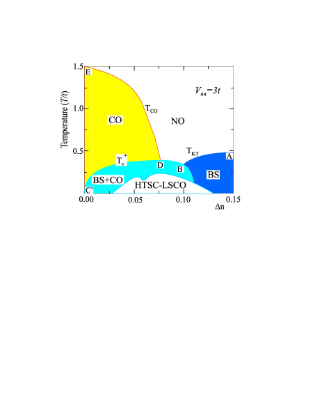
Figure 2: Fig. 2. (Color online) The QMC T-n phase diagram of the 2D hc-boson system (reconstruction of Fig. 2 from Ref.Schmid . Blank painting marks the HTSC phase for LSCO.

Simple uniform EHBL model truly reproduces many important aspects of the cuprate physics, in particular, the pseudogap phenomenon as a result of the charge ordering and high values of the critical temperatures for superconducting transition. Indeed, the phase diagram in Fig. 2 points to critical temperatures for 2D superconductivity as large as 0.5 $t$ that is on the order of 500 K, if we take into account reasonable estimations for the transfer integral in cuprates Moskvin-11 : $t\sim I\sim$ 1000 K. Thus, the model is very promising for finding paths to room-temperature superconductivity Kresin . At the same time the model cannot explain a number of well-known properties, in particular, manifestation of the Cu²⁺ valence states in doped cuprates over wide doping range Johnston and suppression of the superconductivity for overdoped cuprates. Such a behaviour cannot be derived from the EHBL scenario and points to realization of the more complicated ”boson-fermion”  dual XY-Z${}_{FIM}^{123}$ phase with coexisting spin and pseudospin (charge) orders in a wide doping range from parent to overdoped compounds including all the superconducting phase. The suppression of the superconductivity for the hole overdoped cuprates can be explained as a transition from the trivalent superconducting (M¹²³) phase to a bivalent nonsuperconducting M²³ phase. Indeed, the M^-=Cu¹⁺ centers could be energetically gainless under hole doping particularly for overscreened EH coupling. Some properties of nonsuperconducting phases M²³ and M¹², or $XY$-$Z_{FM}^{23}$ and $XY$-$Z_{FM}^{12}$, can be understood if we address limiting insulating phases $M^{+}$ or $M^{-}$ ($Z_{FM}^{1}$ or $Z_{FM}^{3}$) with precisely $M^{+}$ or $M^{-}$-centers on each of the lattice sites. In frames of the pseudospin formalism these phases correspond to fully polarized ferromagnetic states with $S_{z}^{tot}$ = $\pm$ N, where N is the number of Cu sites. Interestingly, in frames of the pseudospin formalism the ”heavily overdoped”  $XY$-$Z_{FM}^{23}$ and $XY$-$Z_{FM}^{12}$ phases with $x\approx$ 1 can be represented as ferromagnets where the charge constraint is realized through the occurrence of $(1-x)N$ non-interacting pseudospin magnons ($\Delta S_{z}$ = $\pm$ 1), that is Cu²⁺ centers, obeying Fermi statistics due to s=1/2 conventional spin. These heavily overdoped cuprates could be addressed to be conventional Fermi liquids. Indeed, the standard Fermi liquid theory hinges on the key assumption that although the electrons (holes) interact, the low-energy excitation spectrum stands in a one-to-one correspondence with that of a non-interacting system. In other words, the Fermi liquid behavior can be typical for overdoped $XY$-$Z_{FM}^{23}$ and $XY$-$Z_{FM}^{12}$ phases in a rather wide range of ”overdoping”. The phases are expected to manifest all the signatures of an $electron$ ($hole$) Fermi liquid with a large Fermi surface which contains $(1-x)$ electrons in the hole-doped cuprates such as La_2-xSr_xCuO₄ or $(1-x)$ holes in the electron-doped cuprates such as Nd_2-xCe_xCuO₄. However, this conventional Fermi liquid behavior can fail for hole or electron overdoped cuprates with a rather large content of Cu²⁺ centers and the electron pairing due to disproportionation reaction Cu²⁺+Cu²⁺$\rightarrow$Cu³⁺+Cu¹⁺ with formation of EH dimers and local bosons. In the framework of the pseudospin formalism we arrive at a binding of two pseudomagnons with $\Delta S_{z}$ = -1 to a single bimagnon $\Delta S_{z}$ = -2. In other words, we may think of the local boson as a long-lived virtual two-pseudomagnon bound state, or bimagnon, where the pseudomagnons are bound on the same site. Electron pairing due to formation of the EH dimers, or CT exciton concept offers a fruitful insight into challenging issues of the copper oxide superconductors Gorkov ; Gorkov-2 ; cofermion ; Phillips . The EH binding/unbinding energy $\Delta_{EH}$, that is the energy of the local boson binding in the EH dimer, can be identified with the pseudogap observed in the extended part of the cuprate phase diagram from heavily underdoped to overdoped systems. On the other hand, this energy defines an effective gap for the thermal activation of hole carriers which has been found from the high-temperature Hall data in La_2-xSr_xCuO₄ Gorkov ; Gorkov-2 ; Ando ; Ono . Effective number of hole carriers derived from $R_{H}(T)$ were excelently fitted by a simple two-component formula where the first component is related with the temperature independent itinerant carriers, while the second one bears the activation character. Interestingly, the activation energy was shown to coincide with the ARPES measured excitation energies needed to transfer electron from the antinodal points (0,$\pi$), ($\pi$, 0) in the Brillouin zone to the chemical potential Gorkov ; Gorkov-2 . The equal energy for creation of an electron (ARPES) and a hole (thermal activation) can be understood only in terms of bound states for electron-hole pairs Gorkov ; Gorkov-2 , EH-dimers, or condensation of the CT excitons whose coupling/decoupling energy is revealed in both types of experiments. These states, seen near antinodal points, according to ARPES, form quasi-periodic structures close to the double periodicity along the Cu-Cu bonds directions. The number of itinerant carriers rapidly increases with $x$ Gorkov ; Gorkov-2 ; Ando ; Ono that results in an effective screening of the $\Delta_{EH}(x)$ parameter with a sharp fall of the ”ionization”  energy of the EH dimers from $\Delta_{EH}(x)\approx$ 0.5 eV given $x$ = 0.01 up to values close to zero given $x>$ 0.2. Given zero values of the $\Delta_{EH}$ parameter the $XY$-$Z_{FIM}^{123}$ phase becomes energetically gainless as compared with $XY$-$Z_{FM}^{23}$ phase, hence we arrive at a QCP separating superconducting $XY$-$Z_{FIM}^{123}$ phase and nonsuperconducting $XY$-$Z_{FM}^{23}$ phase with a large Fermi surface (FS) and other attributes of a Fermi liquid. The onset of the pseudogap below QCP naturally explains the FS reconstruction with a number of unusual properties of the doped cuprates, such as the Fermi arc and/or pocket formation cofermion .

It should be noted that the ”negative-$U$”  model is a limiting case of more complicated model with suppressed single-particle transport but with finite, positive or negative, values of the on-site correlation parameter $U$. Such a model was analyzed recently both within the mean-field approximation and quantum Monte-Carlo calculation Acta .

5 Topological defects in 2D S=1 pseudospin systems

5.1 Short overview

In the framework of our charge triplet model the cuprates prove to be in the universality class of the (pseudo)spin 2D systems whose description incorporates static or dynamic topological defects to be natural element both of micro- and macroscopic physics. Like domain walls, the vortices and skyrmions are stable for topological reasons. Depending on the structure of effective pseudo-spin Hamiltonian in 2D-systems the latter could correspond to either in-plane and out-of-plane vortices or skyrmions BP . Under certain conditions either topological defects could determine the structure of the ground state. In particular, this could be a generic feature of electric multipolar systems with long-range multipolar interactions. Indeed, a Monte-Carlo simulation of a ferromagnetic Heisenberg model with dipolar interaction on a 2D square lattice $L\times L$ shows that, as $L$ is increased, the spin structure changes from a ferromagnetic one to a novel one with a vortex-like arrangement of spins even for rather small magnitude of dipolar anisotropy Sasaki .

Quasi-classical continuous description of the 2D magnetic systems reveals their striking features, namely, the collective localized inhomogeneous states with nontrivial topology and finite excitation energy. These include topological solitons BP ; Voronov1983 , magnon drops Ivanov1977 , in- and out-of-plane vortex-antivortex pairs Gouva1989 , and various spiral solutions Borisov2001 ; Bostrem2002 ; Borisov2004 . Basically these solutions have been obtained for the isotropic and anisotropic ferromagnet.

A vector representation is useful, if not a single instrument of a visual qualitative description of complex spin and pseudospin structures. A striking example of a single-vector representations are the Néel and Bloch domain walls in classic ferromagnets. Situation in quantum S=1 systems is more intricate, however, our ”two-vector”  (${\bf m}$, ${\bf n}$)-description of the on-site S=1 states can be successfully applied to predict and analyse different uniform and nonuniform, in particular, topological structures. One of the most surprising is the prediction of the existence of unusual antiphase $180^{\circ}$-domain walls for parent cuprates. Indeed, the bare on-site Cu²⁺ state in parent cuprate is described by the collinear pair of vectors ${\bf m}$ and ${\bf n}$, or $-{\bf m}$ and $-{\bf n}$ directed along $Z$-axis. It means that two ”parent”  domains can be separated by a domain wall in which a collinear pair of vectors ${\bf m}$ and ${\bf n}$ can rotate by 180 degrees (see Fig. 1). Deviation from $Z$-axis corresponds to emergence of the on-site electron-hole Cu¹⁺-Cu³⁺ component due to the gradual suppression of the bare parent Cu²⁺ component until its complete disappearance in the domain wall center with the maximum value of the electron-hole Cu¹⁺-Cu³⁺ component. which ensures the maximum value of the electron-hole component and, accordingly, the maximum value of the modulus of the superconducting order parameter $\langle{\hat{S}}^{2}_{\pm}\rangle$. In other words, such a domain wall can be considered as a potential source of filamentary superconductivity.

Interestingly, the domain wall structure is characterized by an uniform distribution of the mean on-site charge as $\langle{\hat{S}}_{z}\rangle$ = 0 for collinear (${\bf m}$, ${\bf n}$)-pair. In other words, the domain wall structure and bare parent Cu²⁺ monovalent (insulating) phase have absolutely the same distribution of the mean on-site charges. From the one hand, this point underlines an unconventional quantum nature of the on-site states indomain wall, while from the other hand it makes the domain wall textures to be invisible, in particular, for X-rays.

It is obvious that the formation of such domain walls in the parent cuprates is energetically unfavorable, however, the situation changes radically with electron/hole doping due to the fact that the doping into a domain wall stabilizes the domain configuration bubble ; bubble-2 . The antiphase domain wall in the parent cuprate appears to be a very efficient potential well for the localization of extra electron/hole pairs thus forming a novel type of a neutral or charged topological defect. We believe that the stripe structures in underdoped cuprates Tranquada ; Bianconi ; Zaanen can somehow be associated with these antiphase domain walls.

Topological defects are stable non-uniform spin structures with broken translational symmetry and non-zero topological charge (chirality, vorticity, winding number). Vortices are stable states of anisotropic 2D Heisenberg Hamiltonian

$${\hat{H}}=\sum_{i<j}J_{ij}(S_{ix}S_{jx}+S_{iy}S_{jy}+\lambda S_{iz}S_{jz}),$$ (33)

with the ”easy-plane” anisotropy when the anisotropy parameter $\lambda<1$. Classical in-plane vortex ($S_{z}=0$) appears to be a stable solution of classical Hamiltonian (33) at $\lambda<\lambda_{c}$ ($\lambda_{c}\approx 0.7$ for square lattice). At $1>\lambda>\lambda_{c}$ stable solution corresponds to the out-of-plane OP-vortex ($S_{z}\not=0$), at which center the spin vector appears to be oriented along $z$-axis, and at infinity it arranges within $xy$-plane. The in-plane vortex is described by the formulas $\Phi=q\varphi$, $\cos\theta=0$. The $\theta(r)$ dependence for the out-of-plane vortex cannot be found analytically. Both kinds of vortices have the energy logarithmically dependent on the size of the system.

The cylindrical domains, or bubble like solitons with spins oriented along the $z$-axis both at infinity and in the center (naturally, in opposite directions), exist for the ”easy-axis” anisotropy $\lambda>1$. Their energy has a finite value. Skyrmions are general static solutions of classical continuous limit of the isotropic ($\lambda=1$) 2D Heisenberg ferromagnet, obtained by Belavin and Polyakov BP from classical nonlinear sigma model. Belavin-Polyakov skyrmion and out-of-plane vortex represent the simplest toy model (pseudo)spin textures BP ; Borisov .

The simplest skyrmion spin texture looks like a bubble domain in ferromagnet and consists of a vortex-like arrangement of the in-plane components of spin with the $z$-component reversed in the centre of the skyrmion and gradually increasing to match the homogeneous background at infinity. The spin distribution within such a classical skyrmion with a topological charge $q$ is given as follows BP

$$\Phi=q\varphi+\varphi_{0};\quad\cos\Theta=\frac{r^{2q}-\lambda^{2q}}{r^{2q}+\lambda^{2q}},$$ (34)

where $r,\varphi$ are polar coordinates on plane, $q=\pm 1,\,\pm 2,...$ the chirality. For $q=1$, $\varphi_{0}$ = 0 we arrive at

$$n_{x}=\frac{2r\lambda}{r^{2}+\lambda^{2}}\cos\varphi;\,n_{y}=\frac{2r\lambda}{r^{2}+\lambda^{2}}\sin\varphi;\,n_{z}=\frac{r^{2}-\lambda^{2}}{r^{2}+\lambda^{2}}\,.$$

(35)

In terms of the stereographic variables the skyrmion with radius $\lambda$ and phase $\varphi_{0}$ centered at a point $z_{0}$ is identified with spin distribution $w(z)=\frac{\Lambda}{z-z_{0}}$, where $z=x+iy=re^{i\varphi}$ is a point in the complex plane, $\Lambda=\lambda e^{i\alpha}$. For a multicenter skyrmion we have BP

$$w(z)=\cot\frac{\Theta}{2}\,e^{i\Phi}=\prod_{i}\left(\frac{z-z_{j}}{\Lambda}\right)^{m_{j}}\prod_{j}\left(\frac{\Lambda}{z-z_{j}}\right)^{n_{j}}\,,$$

(36)

where $\sum m_{i}>\sum n_{j}$, $q=\sum m_{j}$. Skyrmions are characterized by the magnitude and sign of its topological charge, by its size (radius), and by the global orientation of the spin. The scale invariance of skyrmionic solution reflects in that its energy $E_{sk}=4\pi|q|IS^{2}$ is proportional to topological charge and does not depend on radius and global phase BP . Like domain walls, vortices and skyrmions are stable for topological reasons. Skyrmions cannot decay into other configurations because of this topological stability no matter how close they are in energy to any other configuration.

In a continuous field model, such as, e.g., the nonlinear $\sigma$-model, the ground-state energy of the skyrmion does not depend on its size BP , however, for the skyrmion on a lattice, the energy depends on its size. This must lead to the collapse of the skyrmion, making it unstable. Strong anisotropic interactions, in particular, long range dipole-dipole interactions may, in principle, dynamically stabilize the skyrmions in 2D lattices Abanov ; Ivanov2006 ; Galkina2009 .

Wave function of the spin system, which corresponds to a classical skyrmion, is a product of spin coherent states Perelomov1986 . In case of spin $S=\frac{1}{2}$

$$\Psi_{sk}(0)=\prod\limits_{i}[\cos\frac{\theta_{i}}{2}e^{i\frac{\varphi_{i}}{2}}\mid\uparrow\rangle+\sin\frac{\theta_{i}}{2}e^{-i\frac{\varphi_{i}}{2}}\mid\downarrow\rangle],$$ (37)

where $\theta_{i}=\arccos\frac{r_{i}^{2}-\lambda^{2}}{r_{i}^{2}+\lambda^{2}}$. Coherent state provides a maximal equivalence to classical state with minimal uncertainty of spin components. The motion of such skyrmions has to be of highly quantum mechanical nature. However, this may involve a semi-classical percolation in the case of heavy non-localized skyrmions or variable range hopping in the case of highly localized skyrmions in a random potential. Effective overlap and transfer integrals for quantum skyrmions are calculated analytically by Istomin and Moskvin Istomin . The skyrmion motion has a cyclotronic character and resembles that of electron in a magnetic field.

The interest in skyrmions in ordered spin systems received much attention soon after the discovery of high-temperature superconductivity in copper oxides skyrmion-cuprates ; skyrmion-cuprates-2 ; skyrmion-cuprates-3 ; skyrmion-cuprates-4 ; skyrmion-cuprates-5 ; skyrmion-cuprates-6 ; skyrmion-cuprates-7 ; skyrmion ; skyrmion-2 ; skyrmion-3 ; skyrmion-4 . Initially, there was some hope that interaction of electrons and holes with spin skyrmions could play some role in superconductivity, but this was never successfully demonstrated. Some indirect evidence of skyrmions in the magnetoresistance of the litium doped lanthanum copper oxide has been recently reported skyrmion-LaLiCuO but direct observation of skyrmions in 2D antiferromagnetic lattices is still lacking. In recent years the skyrmions and exotic skyrmion crystal (SkX) phases have been discussed in connection with a wide range of condensed matter systems including quantum Hall effect, spinor Bose condensates and especially chiral magnets Bogdanov ; Bogdanov-2 ; Nagaosa2013 . It is worth noting that the skyrmion-like structures for hard-core 2D boson system were considered by Moskvin et al. bubble ; bubble-2 in frames of the s=1/2 pseudospin formalism.

5.2 Unconventional skyrmions in S=1 (pseudo)spin systems

Different skyrmion-like topological defects for 2D (pseudo)spin S=1 systems as solutions of isotropic spin Hamiltonians were addressed in Ref. Knig and in more detail in Ref. Nadya . In general, isotropic non-Heisenberg spin-Hamiltonian for the S=1 quantum (pseudo)spin systems should include both bilinear Heisenberg exchange term and biquadratic non-Heisenberg exchange term:

$$\hat{H} = -\tilde{J}_{1}\sum_{i,\eta}\hat{\bf{S}}_{i}\hat{\bf{S}}_{i+\eta}-\tilde{J}_{2}\sum_{i,\eta}(\hat{\bf{S}}_{i}\hat{\bf{S}}_{i+\eta})^{2}=$$

$$= -J_{1}\sum_{i,\eta}\hat{\bf{S}}_{i}\hat{\bf{S}}_{i+\eta}-J_{2}\sum_{i,\eta}\sum_{k\geq j}^{3}(\{\hat{S}_{k}\hat{S}_{j}\}_{i}\{\hat{S}_{k}\hat{S}_{j}\}_{i+\eta}),$$

where $J_{i}$ are the appropriate exchange integrals, $J_{1}=\tilde{J}_{1}-\tilde{J}_{2}/2$, $J_{2}=\tilde{J}_{2}/2$, $i$ and $\eta$ denote the summation over lattice sites and nearest neighbours, respectively.

Having substituted our trial wave function (12) to $\langle{\hat{H}}\rangle$ provided $\langle\hat{\bf S}(1)\hat{\bf S}(2)\rangle=\langle\hat{\bf S}(1)\rangle\langle\hat{\bf S}(2)\rangle$ we arrive at the Hamiltonian of the isotropic classical spin-1 model in the continual approximation as follows:

$$H = J_{1}\int d^{2}{\bf r}\left[\sum_{i=1}^{3}(\vec{\nabla}\langle S_{i}\rangle)^{2}\right]+{}$$ (39)

$${}+J_{2}\int d^{2}{\bf r}\left[\sum_{i\leq j=1}^{3}(\vec{\nabla}a_{i}a_{j}+\vec{\nabla}b_{i}b_{j})^{2}\right]+{}$$

$${}+\frac{4(J_{2}-J_{1})}{c^{2}}\int|\langle\hat{\bf S}\rangle|^{2}d^{2}{\bf r},$$

where $\langle\hat{\bf S}\rangle=2[\bf a\times\bf b]$. It should be noted that the third ”gradientless” term in the Hamiltonian breaks the scaling invariance of the model.

5.2.1 Dipole (pseudo)spin skyrmions

Dipole, or magnetic skyrmions as the solutions of bilinear Heisenberg (pseudo)spin Hamiltonian when $J_{2}=0$ were obtained in Ref. Knig given the restriction $\bf a\perp\bf b$ and the lengths of these vectors were fixed.

The model reduces to the nonlinear O(3)-model with the solutions for $\bf a$ and $\bf b$ described by the following formulas (in polar coordinates):

$$\sqrt{2}{\bf a} = ({\bf e_{z}}\sin\theta-{\bf e}_{r}\cos\theta)\sin\varphi+{\bf e}_{\varphi}\cos\varphi,$$

$$\sqrt{2}{\bf b} = ({\bf e}_{z}\sin\theta-{\bf e}_{r}\cos\theta)\cos\varphi-{\bf e}_{\varphi}\sin\varphi.$$ (40)

For dipole ”magneto-electric” skyrmions the $\bf m,\bf n$ vectors are assumed to be perpendicular to each other ($\bf m\perp\bf n$) and the (pseudo)spin structure is determined by the skyrmionic distribution (34) of the ${\bf l}=[{\bf m}\times{\bf n}]$ vector Knig . In other words, the fixed-length spin vector $\langle{\bf S}\rangle=2[{\bf a}\times{\bf b}]$ is distributed in the same way as in the usual skyrmions (34). However, unlike the usual classic skyrmions, the dipole skyrmions in the S=1 theory have additional topological structure due to the existence of two vectors $\bf m$ and $\bf n$. Going around the center of the skyrmion the vectors can make $N$ turns around the ${\bf l}$ vector. Thus, we can introduce two topological quantum numbers: $N$ and $q$ Knig . In addition, it should be noted that $q$ number may be half-integer. The dipole-quadrupole skyrmion is characterized by nonzero both pseudospin dipole order parameter $\langle\bf S\rangle$ with usual skyrmion texture (34) and quadrupole order parameters

$$\langle\{{\hat{S}}_{i}{\hat{S}}_{j}\}\rangle=2\langle{\hat{S}}_{i}\rangle\langle{\hat{S}}_{j}\rangle=l_{i}l_{j}.$$ (41)

5.2.2 Quadrupole (pseudo)spin skyrmions

Hereafter we address another situation with purely biquadratic (pseudo)spin Hamiltonian ($J_{1}$=0) and treat the non-magnetic (“electric”) degrees of freedom. The topological classification of the purely electric solutions is simple because it is also based on the usage of subgroup instead of the full group. We address the solutions given $\vec{a}\parallel\vec{b}$ and the fixed lengths of the vectors, so we use for the classification the same subgroup as above.

After simple algebra the biquadratic part of the Hamiltonian can be reduced to the expression familiar for nonlinear O(3)-model:

$$H_{bq} = J_{2}\int d^{2}{\bf r}\left[\sum_{i,j=1}^{3}(\vec{\nabla}n_{i}n_{j})^{2}\right]={}$$ (42)

$$= 2J_{2}|{\bf n}|^{2}\int d^{2}{\bf r}\left[\sum_{i=1}^{3}(\vec{\nabla}n_{i})^{2}\right],$$

where ${\bf a}=\alpha{\bf n},{\bf b}=\beta{\bf n}$, and $\alpha+i\beta=\exp(i\kappa)$, $\kappa\in R$, $|{\bf n}|^{2}=$const. Its solutions are skyrmions, but instead of the spin distribution in magnetic skyrmion we have solutions with zero spin, but the non-zero distribution of five spin-quadrupole moments $Q_{ij}$, or $\langle\{S_{i}S_{j}\}\rangle$ which in turn are determined by the ”skyrmionic”  distribution of the ${\bf n}$ vector (34) with classical skyrmion energy: $E_{el}=16\pi qJ_{2}$. The distribution of the spin-quadrupole moments $\langle\{S_{i}S_{j}\}\rangle$ can be easily obtained:

$$\langle S_{z}^{2}\rangle=\frac{4r^{2q}\lambda^{2q}}{(r^{2q}+\lambda^{2q})^{2}},\;\langle{\hat{S}}_{\pm}^{2}\rangle=\frac{2r^{2q}\lambda^{2q}}{(r^{2q}+\lambda^{2q})^{2}}e^{\pm 2iq\varphi},$$

$$\langle{\hat{T}}_{\pm}\rangle=-i\sqrt{2}\frac{(\lambda^{2q}-r^{2q})r^{q}\lambda^{q}}{(r^{2q}+\lambda^{2q})^{2}}e^{\mp iq\varphi}.$$ (43)

One should be emphasized that the distribution of five independent quadrupole order parameters for the quadrupole skyrmion are straightforwardly determined by a single vector field ${\bf m}({\bf r})$ (${\bf n}({\bf r})$) while $\langle\hat{\bf S}\rangle$ = 0.

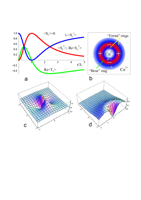
Figure 3: (Color online) a) Radial distribution of the diagonal and off-diagonal nematic order parameters (the Cu²⁺ spin density, the modulus of the SC order parameter, and the $T$-type order parameter) for a quadrupole pseudospin skyrmion (q=1): b) the ring shaped distribution of the Cu²⁺ spin density and off-diagonal order parameters describing the Fermi- and Bose-like transport, arrows point to opposite sign of the $T$-type order parameter for the ”internal”  and ”external”  rings, the $\pm$ signs point to the signs of the $Re\langle{\hat{S}}_{\pm}^{2}\rangle$: c) and d) the spatial distribution of $Re\langle{\hat{S}}_{\pm}^{2}\rangle$ and $\langle{\hat{S}}_{z}^{2}\rangle$, respectively. It should be noted the $d_{x^{2}-y^{2}}$ symmetry of the SC order parameter.

The quadrupole skyrmion supposedly can be a typical topological charge excitation for parent or underdoped cuprates. Fig.3 demonstrates the radial distribution of different order parameters for the quadrupole skyrmion, the modulus of the SC order parameter, the Cu²⁺ spin density, and the $T$-type order parameter. We see a circular layered structure with clearly visible anticorrelation effects due to a pseudospin kinematics. Interestingly, at the center ($r=0$) and far from the center ($r\rightarrow\infty$) for such a skyrmion we deal with a parent Cu²⁺ monovalent (insulating) state while for the domain wall center ($r=\lambda$) we arrive at a fully disproportionated ”superconducting”   Cu¹⁺-Cu³⁺ superposition whose weight diminishes with moving away from the center. In other words, the ring shaped domain wall is an area with a circular distribution of the superconducting order parameter, or circular ”bosonic”  supercurrent. Nonzero $T$-type order parameter distribution points to a circular ”fermionic” current with a puzzlingly opposite sign of the $\langle{\hat{T}}_{\pm}\rangle$ parameter for ”internal”  ($0<r<\lambda$) and ”external”  ($r>\lambda$) parts of the skyrmion. Given the simplest winding number $q=1$ we arrive at the $d$-wave ($d_{x^{2}-y^{2}}$/$d_{xy}$ symmetry of the superconducting order parameter.

First of all we should note that such a skyrmionic structure is characterized by an uniform distribution of the mean on-site charge as $\langle{\hat{S}}_{z}\rangle$ = 0, that is why it can be termed as a neutral skyrmion. Indeed, all over the skyrmion the ${\bf m}$ and ${\bf n}$ vectors form a collinear configuration, thus $\langle{\bf S}\rangle$ turns into zero. In other words, the quadrupole skyrmionic structure and bare parent Cu²⁺ monovalent (insulating) phase have absolutely the same distribution of the mean on-site charges. From the one hand, this point underlines an unconventional quantum nature of the quadrupole skyrmion under consideration, while from the other hand it makes the quadrupole skyrmion texture to be invisible, in particular, for X-rays. At the same time, the skyrmion has a well developed layered ring-shaped distribution of the $\langle{\hat{T}}_{\pm}\rangle$ and $\langle{\hat{S}}_{\pm}^{2}\rangle$ order parameters that points to its instability with regard to circular fermionic- and bosonic-like circular currents with maximal current density around the skyrmion radius. In this connection it is worth noting a scenario of the circulating charge currents for underdoped cuprates Varma ; JETPLett-12 .

An interesting example of a topological inhomogeneity is provided by a multi-center skyrmion BP which energy does not depend on the position of the centers. The latter are believed to be addressed as an additional degree of freedom, or positional order parameter. Fig. 4 shows an example of the in-plane distribution of the modulus of the SC order parameter $\langle{\hat{S}}^{2}_{\pm}\rangle$ for a multi-center quadrupole pseudospin skyrmion with a random distribution of the centers. An individual skyrmion in this multi-center entity can be characterized by its position (i.e., the center of a skyrmionic texture), its size (i.e., the radius of domain wall), and the orientation of the in-plane components of pseudospin (U(1) degree of freedom).

The domain wall center of the quadrupole skyrmion provides maximal values of the pseudospin susceptibility $\chi_{zz}$, or charge susceptibility bubble ; bubble-2 . It means the domain wall appears to form a very efficient ring-shaped potential well for the charge carrier localization thus giving rise to a novel type of a charged topological defect. In the framework of the pseudospin formalism the skyrmion charging corresponds to a single-magnon $\Delta S_{z}$ = $\pm$ 1 (single particle) or a two-magnon $\Delta S_{z}$ = $\pm$ 2 (two-particle) excitations. It is worth noting that for large negative $\Delta$ the single-magnon (single-particle) excitations may not be the lowest energy excitations of the strongly anisotropic pseudospin system. Their energy may surpass the energy of a two-magnon bound state (bimagnon), or two-particle, local boson-like, excitation, created at a particular site. Thus we arrive at a competition of the two types of charged quadrupole skyrmions. Such a charged topological defect can be addressed to be an extended skyrmion-like mobile quasiparticle. However, at the same time it should’nt be forgotten that skyrmion corresponds to a collective state (excitation) of the whole system.

Skyrmionic scenario allows us to make several important predictions for cuprates. First, the parent insulating antiferromagnetic monovalent Cu²⁺ phase may be unstable with regard to nucleation of a topological defect in the unconventional form of a single- or multi-center skyrmion-like object with ring-shaped superfluid regions. The parent Cu²⁺ phase may gradually lose its stability under non-isovalent substitution (electron/hole doping), while a novel topological self-organized texture is believed to become stable. The most probable possibility is that every domain wall accumulates single boson, or boson hole. Then, the number of centers in a multi-center skyrmion nucleated with doping has to be equal to the number of bosons/holes. In such a case, we anticipate the near-linear dependence of the total SC volume fraction on the doping. Generally speaking, one may assume scenario when the nucleation of a multi-center skyrmion occurs spontaneously with no doping. In such a case we should anticipate the existence of neutral multi-center skyrmion-like object with equal number of positively and negatively charged single skyrmions. However, in practice, namely the boson/hole doping is likely to be a physically clear driving force for a nucleation of a multi-center skyrmion-like self-organized collective mode which may be (not strictly correctly) referred to as multi-skyrmion system akin in a quantum Hall ferromagnetic state of a two-dimensional electron gas Green . It seems likely that for a light doping any doped particle results in a nucleation of a new single-skyrmion state, hence its density changes gradually with particle doping. Therefore, as long as the separation between skyrmionic centers is sufficiently large so that the inter-skyrmion coupling is negligible, the energy of the system per particle remains almost constant. This means that the chemical potential remains unchanged with doping.

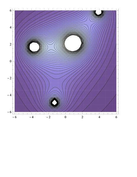
Figure 4: Contour plot of the in-plane distribution of the modulus of the off-diagonal SC order parameter $\langle{\hat{S}}^{2}_{\pm}\rangle$ for a multicenter quadrupole pseudospin skyrmion with a random distribution of the centers.

Nucleation of the skyrmionic textures eventually leads to the destruction of the antiferromagnetic Neél ordering which is known to exist even at very low doping. Furthermore, the skyrmion structure with insulating spin s=1/2 core isolated by spinless nonmagnetic Cu¹⁺-Cu³⁺ ring-shaped domain wall from surrounding Cu²⁺ entity provides a physically clear mechanism of the nucleation of a spin glass phase typical for underdoped cuprates. Furthermore, the nucleation of the unconventional quadrupole skyrmions does provide a physically clear mechanism for the unconventional vortex Nernst signal and local diamagnetism universally observed in many hole doped cuprates at the temperatures above T_c Nernst .

Meanwhile we discuss the quadrupole skyrmion to be a classical solution of the continual isotropic model, however, this idealized object is believed to preserve their main features for strongly anisotropic (pseudo)spin lattice quantum systems. Both quantum effects and the discreteness of skyrmion texture can result in substantial deviations from the predictions of a classical model. The continuous model is relevant for discrete lattices only if we deal with long-wave length inhomogeneities when their size is much bigger than the lattice spacing. In the discrete lattice the very notion of topological excitation seems to be inconsistent. At the same time, the discreteness of the lattice itself does not prohibit from considering the nanoscale (pseudo)spin textures whose topology and spin arrangement is that of a skyrmion skyrmion-cuprates-6 . It is worth to note that skyrmions cannot decay into other configurations because of the topological stability no matter how close they are in energy to any other configuration.

The boson addition or removal in the half-filled ($n=1$) boson system can be a driving force for a nucleation of a multi-center “charged” skyrmions. Such topological structures, rather than uniform phases predicted by the mean-field approximation, are believed to describe the evolution of the EBHM systems away from half-filling. It is worth noting that the multi-center skyrmions one considers as systems of skyrmion-like quasiparticles forming skyrmion liquids and skyrmion lattices, or crystals (see, e.g., Refs. Timm ; Green ).

5.2.3 Dipole-quadrupole (pseudo)spin skyrmions

In the continual limit for $J_{1}=J_{2}=J$ the Hamiltonian (39) can be transformed into the classical Hamiltonian of the fully $SU(3)$-symmetric scale-invariant model which can be rewritten as follows Nadya :

$$H_{isotr}=2J\int d^{2}{\bf r}\{(\vec{\nabla}\Theta)^{2}+\sin^{2}\Theta(\vec{\nabla}\eta)^{2}+{}$$

$${}+\sin^{2}\Theta\cos^{2}\Theta\left[\cos^{2}\eta(\vec{\nabla}\Psi_{1})^{2}+\sin^{2}\eta(\vec{\nabla}\Psi_{2})^{2}\right]+{}$$

$${}+\sin^{4}\Theta\cos^{2}\eta\sin^{2}\eta(\vec{\nabla}\Psi_{1}-\vec{\nabla}\Psi_{2})^{2}\},$$ (44)

where we have used the representation (10) and introduced $\Psi_{1}=\Phi_{1}-\Phi_{3},\Psi_{2}=\Phi_{3}-\Phi_{2}$. The topological solutions for the Hamiltonian (44) can be classified at least by three topological quantum numbers (winding numbers): phases $\eta,\Psi_{1,2}$ can change by $2\pi$ after the passing around the center of the defect. The appropriate modes may have very complicated topological structure due to the possibility for one defect to have several different centers (while one of the phases $\eta,\Psi_{1,2,3}$ changes by $2\pi$ given one turnover around one center $(r_{1},\varphi_{1})$, other phases may pass around other centers $(r_{i},\varphi_{i})$). It should be noted that for such a center the winding numbers may take half-integer values. Thus we arrive at a large variety of topological structures to be solutions of the model. Below we will briefly address two simplest classes of such solutions. One type of skyrmions can be obtained given the trivial phases $\Psi_{1,2}$. If these are constant, the ${\bf R}$ vector distribution (see (10)) represents the skyrmion described by the usual formula (34). All but one topological quantum numbers are zero for this class of solutions. It includes both dipole and quadrupole solutions: depending on selected constant phases one can obtain both ”electric” and different ”magnetic” skyrmions. The substitution $\Phi_{1}=\Phi_{2}=\Phi_{3}$ leads to the electric skyrmion which was obtained above as a solution of more general SU(3)-anisotropic model. Another example can be $\Phi_{1}=\Phi_{2}=0,\Phi_{3}=\pi/2$. This substitution implies ${\bf b}\|Oz,{\bf a}\|Oxy,{\bf S}\|Oxy$, and ${\bf S}=\sin\Theta\cos\Theta\{\sin\eta,-\cos\eta,0\}$. Nominally, this is the in-plane spin vortex with a varying length of the spin vector

$$|S|=\frac{2r\lambda|r^{2}-\lambda^{2}|}{(r^{2}+\lambda^{2})^{2}},$$ (45)

which is zero at the circle $r=\lambda$, at the center $r=0$ and at the infinity $r\rightarrow\infty$, and has maxima at $r=\lambda(\sqrt{2}\pm 1)$. In addition to the non-zero in-plane components of spin-dipole moment $\langle S_{x,y}\rangle$ this vortex is characterized by a non-zero distribution of (pseudo)spin-quadrupole moments. Here we would like to emphasize the difference between spin-1/2 systems in which there are such the solutions as in-plane vortices with the energy having a well-known logarithmic dependence on the size of the system and fixed spin length, and spin-1 systems in which the in-plane vortices also can exist but they may have a finite energy and a varying spin length. The distribution of quadrupole components associated with in-plane spin-1 vortex is non-trivial. Such solutions can be termed as ”in-plane dipole-quadrupole skyrmions”.

Other types of the simplest solutions with the phases $\Psi_{1}=Q_{1}\varphi,\Psi_{2}=Q_{2}\varphi$ governed by two integer winding numbers $Q_{1,2}$ and $\eta=\eta(r),\Theta=\Theta(r)$ are considered in Ref. Nadya .

6 Topological excitations in ”negative-$U$”  model

6.1 Quasi-classical approximation

Let start with the Hamiltonian of the ”negative-$U$”  model in terms of the pseudospin $\vec{\sigma}$, $\sigma_{z}=\pm 1$:

$$H=-t\sum_{\left\langle ij\right\rangle}\big{(}\sigma_{i+}\sigma_{j-}+\sigma_{i-}\sigma_{j+}\big{)}+V\sum_{\left\langle ij\right\rangle}\sigma_{iz}\sigma_{jz}.$$ (46)

Here $\sigma_{\alpha}$, $\alpha=x,y,z$ are Pauli matrices, $\sigma_{\pm}=(\sigma_{x}\pm i\sigma_{y})/2$. The $z$-component of the pseudospin describes the local density of composite bosons, so that antiferromagnetic $z$-$z$ exchange corresponds to the repulsive density-density interaction, while isotropic ferromagnetic planar exchange corresponds to the kinetic energy of the bosons. The constant total number of the bosons leads to the constraint on the total $z$-component of the pseudospin. We define the $n$, as the density of the total doped charge counted from the state with a zero total z-component, or parent Cu²⁺ state. Then $n$ is the sum of $z$-components of the pseudospin: $\sum_{i}\sigma_{iz}=nN$, where $N$ is the total number of sites. If $\rho$ is the density of hc bosons, then $n$ is the deviation from the half-filling: $\rho=(1+n)/2$.

The energy functional $E=\left\langle\Psi\left|H\right|\Psi\right\rangle$ in a quasi-classical approximation with

$$\left|\Psi\right\rangle=\prod_{i}\left(\cos\frac{\theta_{i}}{2}\,e^{-i\frac{\phi_{i}}{2}}\,|{+}1\rangle+\sin\frac{\theta_{i}}{2}\,e^{i\frac{\phi_{i}}{2}}\,|{-}1\rangle\right),$$ (47)

where $|\pm 1\rangle$ are the eigenfunctions of the $\sigma_{z}$ on $i$-th site, takes the form

$$\varepsilon = -\sum_{\langle ij\rangle}\sin\theta_{i}\,\sin\theta_{j}\,\cos(\phi_{i}-\phi_{j})+{}$$

$${}+\lambda\sum_{\langle ij\rangle}\cos\theta_{i}\,\cos\theta_{j}-\xi\Big{(}\sum_{i}\cos\theta_{i}-nN\Big{)}.$$

Here $\left\langle i,j\right\rangle$ denotes summation over nearest neighbors in a square lattice. The $\theta_{i}$ and $\phi_{i}$ are the polar and azimuthal angles of the quasiclassical pseudospin vector at an $i$-th site. We define $\varepsilon=2{E}/t$, $\lambda=2V/t$, $\xi=2\mu/t$, where the chemical potential $\mu$ takes into account the bosons density constraint.

Hereafter, we introduce two sublattices $A$ and $B$ with the checkerboard ordering. The first sum in the Exp.(6.1) has its lowest value if ${\cos(\phi_{i}-\phi_{j})=1}$. This allows us to make a simplifying assumption, that $\phi_{A}(\vec{r})=\phi_{B}(\vec{r})\equiv\phi(\vec{r})$. It is worth to note that this assumption is confirmed by the results of our numerical simulations. We define functions $u(\vec{r})\equiv\theta_{A}(\vec{r})$, $v(\vec{r})\equiv\theta_{B}(\vec{r})$, and their combinations $f=\cos u\cos v$, $F=-f+\lambda f_{uv}$, where subscripts $u$ and $v$ denote derivatives with respect to these quantities. Then the Euler equations in the continuous approximation take a compact form

$$\left\{\begin{array}[]{l}f_{uv}\phi_{kk}-2f_{v}u_{k}\phi_{k}=0,\\ f_{uv}\phi_{kk}-2f_{u}v_{k}\phi_{k}=0,\\ \displaystyle Fu_{kk}+F_{u}u_{k}u_{k}-f_{u}\phi_{k}\phi_{k}-4F_{u}+\xi\,\sin v=0,\\ \displaystyle Fv_{kk}+F_{v}v_{k}v_{k}-f_{v}\phi_{k}\phi_{k}-4F_{v}+\xi\,\sin u=0.\end{array}\right.$$ (49)

Here we assume summation over pair indices. These equations need to add the boson density constraint. With the relevant exchange constants, the equations (49) lead to the equations of Ref. Egorov2002 .

6.2 The asymptotic behavior of localized solutions

The system (49) along with the boson density constraint has uniform solutions, $\phi=\phi_{0}$, $u=u_{0}$, $v=v_{0}$, that determine the well-known ground-state phase diagram RMP of the hc boson system in the mean-field approximation.

Given $\lambda<1$ or $n^{2}>(\lambda-1)/(\lambda+1)$ the ground state of the system is a superfluid (SF) with $\cos u_{0}=\cos v_{0}=n$, $\varepsilon_{0}=-2+2\left(\lambda+1\right)n^{2}$. Given $n^{2}<(\lambda-1)/(\lambda+1)$ the ground state is a supersolid (SS) with $\cos u_{0}=n+z$, $\cos v_{0}=n-z$, where $z^{2}=1+n^{2}-2|n|\lambda/\sqrt{\lambda^{2}-1}$, and $\varepsilon_{0}=-2\lambda+4|n|\sqrt{\lambda^{2}-1}$. In all phases, the value of $\xi$ satisfies the regular expression $\xi_{0}=\partial\varepsilon_{0}/\partial n$. When $\lambda>1$ and $n=0$ the SS phase transforms into a conventional charge ordered (CO) phase with the checkerboard ordering.

The equations (49) in the case of $\lambda<0$ have localized solutions with nonzero topological charge and finite energy BP ; Voronov1983 ; Ivanov1977 ; Gouva1989 ; Borisov2001 ; Bostrem2002 ; Borisov2004 . However, in our case $\lambda>0$, the numerical calculations with the conjugate gradient method for minimizing of the energy functional (47) on the lattice 256$\times$256 indicate the existence of similar solutions, at least, as metastable states. The results are shown in Fig.5. The actual stability of these solutions in our calculation was different. The SF-phase solutions, similar to that of in Fig.5, cases a and b, quickly evolved to an uniform one. The SS- and CO-phase solutions, similar to that of in Fig.4, cases c and d, retained its form for more than $10^{6}$ iterations.

We investigated the asymptotic behavior of localized solutions, suggesting that at $r\rightarrow\infty$ they have the form $\phi(\vec{r})=\phi_{0}+\tilde{\phi}(\vec{r})$, $u(\vec{r})=u_{0}+\tilde{u}(\vec{r})$, $v(\vec{r})=v_{0}+\tilde{v}(\vec{r})$, where $\tilde{\phi},\tilde{u},\tilde{v}\rightarrow 0$ at $r\rightarrow\infty$. Hereinafter, the index 0 means the corresponding values for constant solutions. The linearized system (49) for the functions $\tilde{\phi},\tilde{u},\tilde{v}$ takes the form

$$\left\{\begin{array}[]{l}\displaystyle f_{uv0}\,\tilde{\phi}_{kk}=0,\\ \displaystyle F_{0}\,\tilde{u}_{kk}+4F_{0}\tilde{u}+4\left(-F_{uv0}+\frac{\xi_{0}}{4}\cos v_{0}\right)\tilde{v}=0,\\ \displaystyle F_{0}\,\tilde{v}_{kk}+4F_{0}\tilde{v}+4\left(-F_{uv0}+\frac{\xi_{0}}{4}\cos u_{0}\right)\tilde{u}=0.\end{array}\right.$$ (50)

In the case of the SF and SS phases, the solutions for the first equation can be written as

$$\tilde{\phi}(\vec{r})=\sum_{m=1}^{\infty}\frac{c_{m}}{r^{m}}\cos m(\varphi-\varphi_{m}),$$ (51)

with $c_{m}$ and $\varphi_{m}$ determined by the boundary conditions. In the case of the CO phase, the first equation reduces to an identity since $f_{uv0}=0$.

In the case of the SF phase, the second and the third equations become independent Helmholtz equations for the ferro- and antiferro-type combinations $U=\tilde{u}+\tilde{v}$, $V=\tilde{u}-\tilde{v}$:

$$U_{kk}+A_{1}\,U=0,\quad A_{1}=4\frac{(\lambda+1)(1-n^{2})}{\lambda-(\lambda+1)n^{2}};$$ (52)

$$V_{kk}+A_{2}\,V=0,\quad A_{2}=4\frac{\lambda-1-(\lambda+1)n^{2}}{\lambda-(\lambda+1)n^{2}}.$$ (53)

The corresponding solutions have the form

$$\Phi(\vec{r},r_{i}) = \sum_{l=0}^{\infty}a_{l}K_{l}(r/r_{i})\cos l(\varphi-\alpha_{l}),$$ (54)

$$\Psi(\vec{r},r_{i}) = \sum_{l=0}^{\infty}\Big{[}b_{1l}J_{l}(r/r_{i})\cos l(\varphi-\beta_{1l})+{}$$ (55)

$${}+b_{2l}Y_{l}(r/r_{i})\cos l(\varphi-\beta_{2l})\Big{]},$$

where $K_{l}$ are the Macdonald functions, $J_{l}$ and $Y_{l}$ are the Bessel functions of the first and second kind, and $a_{l}$, $\alpha_{l}$, $b_{kl}$, $\beta_{kl}$, $k=1,2$ are some constants. An analysis of the asymptotic behavior of solutions (54,55) and the requirement that the omitted nonlinear terms in equations (50) are small as compared with the remaining linear terms point to $\Psi=0$. The account in the lowest order of the mixing with the function $\tilde{\phi}$ does not change $V(\vec{r})$ and gives additional term in $U(\vec{r})$ having asymptotic behavior:

$$U_{1}(\vec{r})\approx-\frac{nc_{m}^{2}}{2(\lambda+1)\sqrt{1-n^{2}}}\frac{m^{2}}{r^{2m+2}},$$ (56)

where $m$ is the number that specifies first nonzero term in (51).

Line $n^{2}=\lambda/(\lambda+1)$ is the boundary of areas of the SF-phase with a different behavior of the $U$ and $V$ functions

$$n^{2}>\frac{\lambda}{\lambda+1}:\;U(\vec{r})=\Phi(\vec{r},r_{1})+U_{1}(\vec{r}),\;V(\vec{r})=0;$$ (57)

$$n^{2}<\frac{\lambda}{\lambda+1}:\;U(\vec{r})=U_{1}(\vec{r}),\;\;V(\vec{r})=\Phi(\vec{r},r_{2}).\quad\;$$ (58)

Here we define characteristic lengths $r_{i}^{-2}=|A_{i}|$.

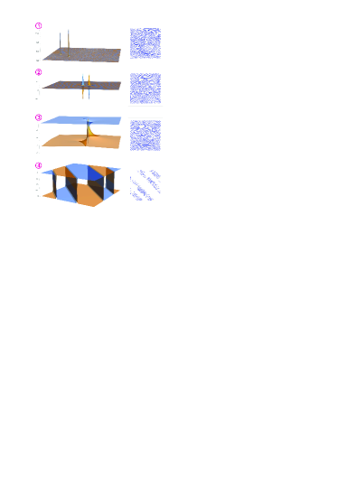
Figure 5: (color online) Nonuniform states in 2D system of charged hard-core bosons. The left panels show local charge density $n_{i}=\sigma_{zi}=\cos\theta_{i}$. The difference of sublattice states is clearly evident in the cases b, c and d. The right panels show phase flow of planar components of the pseudospin, $\sigma_{xi}$ and $\sigma_{yi}$. The phase flow reveals the vortex-antivortex pair structure in the core of inhomogeneity of the local charge density in the cases a, b and c. The parameters of the model are: a) $n=0.2$, $\lambda=0.5$ (SF phase); b) $n=0.1$, $\lambda=0.9$ (SF phase); c) $n=0.2$, $\lambda=1.5$ (SS phase); d) $n=0.0$, $\lambda=1.5$ (CO phase). These sets of parameters are denoted with letters a-d on the ground-state phase diagram in Fig.6.

In the case of the SS phase, we need to define the ferri-type combinations: $\tilde{U}=A\tilde{u}+\tilde{v}$ and $\tilde{V}=A\tilde{u}-\tilde{v}$, where $A=-F_{uv0}+\frac{\xi_{0}}{4}\cos u_{0}$. The equations (50) lead to Helmholtz equation for the $\tilde{U}$ function having solution $\Psi(\vec{r},r_{3})$, $r_{3}^{-2}=8$. As in previous case we have to put $\Psi=0$. The $\tilde{V}$ function obeys the Laplace equation. Taking into account the mixing in the lowest order with the function $\tilde{\phi}$ we come to the expressions as follows

$$\tilde{U}(\vec{r})=\frac{c_{m}^{2}}{8}\left(Af_{u0}+f_{v0}\right)\frac{m^{2}}{r^{2m+2}},$$ (59)

$$\tilde{V}(\vec{r}) = \sum_{l=1}^{\infty}\frac{C_{l}}{r^{l}}\cos l(\varphi-\gamma_{l})+{}$$ (60)

$${}+\frac{c_{m}^{2}}{4}\left(Af_{u0}-f_{v0}\right)\frac{1}{r^{2m}},$$

where $m$ is the number that specifies first non-zero term in (51), and the expressions $f_{u0}=-\sin u_{0}\cos v_{0}$, $f_{v0}=-\cos u_{0}\sin v_{0}$ are determined by the expressions for the uniform solutions.

Similarly the case of the CO phase, we obtain

$$\tilde{\phi}(\vec{r})=0,\quad U(\vec{r})=0,\quad V(\vec{r})=\Phi(\vec{r},r_{4}),$$ (61)

where $r_{4}^{-2}=4(\lambda-1)$.

The analysis of the asymptotic behavior of the localized states reveals qualitative differences of the finite energy excitations in the SF, SS, and CO phases.

In the SF phase an asymptotic of the polar angle of the pseudospin vector is determined by the expressions (57, 58). When comparing these results with numerical calculations it is worth to note that the characteristic lengths obey to inequality $r_{i}<1$ in the most part of the phase diagram in the SF phase except for the areas indicated shadowed in Fig.6, so the function $\Phi$ goes to zero value very fast with increasing of $r$. On the contrary, the asymptotic behavior of the azimuthal angle of the pseudospin (51) has no characteristic scale. This means that in the SF phase the main excitations are almost in-plane vortex-antivortex pairs. They have well localized out-of-plane core of the ferro-type, with $\sigma_{zA}=\sigma_{zB}$, as shown in Fig.5a, and become the pure in-plane ones at $n=0$ in accordance with expression (56). The same type of localized solutions was found by the authors of Ref. Gouva1989 .

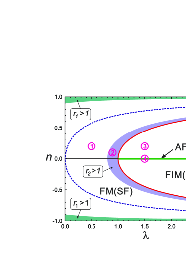
Figure 6: (color online) The ground state phase diagram of the hc bosons in the mean-field approximation. The solid line corresponds to SF-SS phase boundary, $n^{2}=(\lambda-1)/(\lambda+1)$. The thick line at $\lambda>1$, $n=0$ shows CO phase. The dotted line, $n^{2}=\lambda/(\lambda+1)$, separates the two types of the asymptotic behavior in accordance with the expressions (57) and (58). In the shaded areas inside the SF phase region the characteristic lengths satisfy to inequalities $r_{i}>1$. The letters a-d in the circles correspond to the parameter sets in Fig.5.

For the hc bosons, the polar angle is related with the density of bosons, while the azimuthal angle is responsible for the superfluid density, hence these states correspond to the excitation of the superfluid component with highly localized heterogeneity of bosons density in the foci of the vortex-antivortex pairs. In the shaded region in the SF phase near the border of the SF-SS phases in Fig.6, the antiferro type vortices (see Fig.5b), with $\sigma_{zA}\neq\sigma_{zB}$, begin to dominate, their inflation is preceded by a change of the homogeneous ground state from SF to SS phase.

The CO phase has no linear excitation of $\tilde{\phi}$. The characteristic lengths of the azimuthal excitations (61) are small except the region near $\lambda=1$. This results in a high stability of the homogeneous CO phase. A typical picture of the nonuniform state shown in Fig.5d is represented by linear domains of the CO phase. The non-zero values of the SF order parameter are realized within the domain walls, thus giving rise to appearance of a filamentary superfluidity for hc bosons.

In the SS phase the asymptotic behavior of the polar and azimuthal excitations is qualitatively the same without characteristic scales. Hence in this case there are skyrmion-like excitations as shown in Fig.5c. For the hc bosons these coherent states include both the excitations of the superfluid component and the boson density. In a center of skyrmion the difference $\sigma_{zA}-\sigma_{zB}$ has maximal magnitude, that corresponds to CO phase, and near there is a region where $\sigma_{zA}-\sigma_{zB}=0$, that corresponds to SF phase. So, the skyrmion-like excitations in the SS phase generate the topological phase separation. Note, that another type of instability in SS phase were also found by Quantum Monte Carlo calculations Batrouni2000 .

6.3 Computer simulation of the domain structures

Making use of a special algorithm for CUDA architecture for NVIDIA graphics cards that implies a nonlinear conjugate-gradient method to minimize energy functional and Monte-Carlo technique we have been able to directly observe formation of the ground state configuration for the 2D hard-core bosons with lowering the temperature and its transformation with increase the temperature and boson concentration, allowing us to examine earlier implications and uncover novel features of the phase transitions, in particular, look upon the nucleation of the odd domain structure, the localization of the bosons doped away from half-filling, and the phase separation regime. The accuracy of numerical calculations has been limited making it possible to reproduce the effect of minor inhomogeneities common to any real crystal.

We started with the hard-core boson Hamiltonian (30) on a 256$\times$256 square lattice at half-filling ($n\,{=}\,1/2$) given the value of the inter-site repulsion $V_{nn}=V=3t_{nn}$, which is the typical one for many papers with QMC calculations for 2D hard-core bosons Batrouni2000 ; Hebert2001 ; Schmid . It should be noted that hereafter we follow the notations in these papers.

First, we addressed the formation of the phase state under the annealing (thermalization) procedure. The algorithm starts initially with $T$ set to a high value $T\sim 2T_{cr}$. The annealing is accompanied by formation a fragile unstable CO domain structure with antiphase 180^∘ domain walls whose center is characterized by a large nonzero SF order parameter which is suppressed as one runs deep into the CO domain thus suggesting the presence of a fragile filamentary superfluidity (FLSF) nucleated at the antiphase domain walls. The term ”filamentary superfluidity” is a full analogue of a more familiar term ”filamentary superconductivity”. Here, in the paper, ”filamentary superfluidity” is related with an antiphase domain wall (the wall between two CO domains) which is characterized by a nonzero superfluid order parameter.

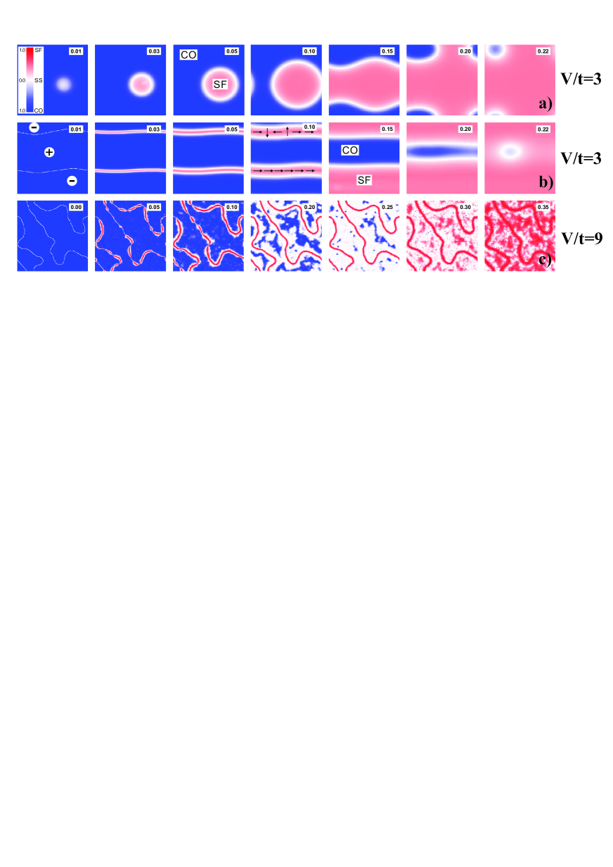
Figure 7: (Color online) Evolution of the hc-boson ground state configuration under doping away from half-filling. a) At $\Delta n$ = 0.01 one observes a sudden nucleation of a rather large ”blob” composed of a SF core and a ring shaped SS boundary that does accommodate all the ”injected” bosons. Under further deviation from half-filling the blob grows up to a full CO-SF phase transformation close to a critical value of $\Delta n$ = 0.225; b) Doped bosons do localize in narrow FLSF DWs of the striped CO phase leading to their broadening. In a well developed phase separation regime we arrive at a system of nearly parallel CO and SF domains separated by the SS DWs. The ”plus”  and ”minus”  signs point to different CO domains. Orientation of the phase angle $\varphi$ within domain walls is demonstrated schematically for $\Delta n$ = 0.1.; c) At $\Delta n$ $<$ 0.01 the doped bosons do localize in the center of the narrow DWs breaking the FLSF without any visible transformation of the domains. The regular DW shape breaks under further doping, these are nonuniformly ”swelled” with the emergence and rise of widenings. Step by step these widenings and ”blobs” nucleated inside domains spread until these cover all lattice. The CO domain topology survives up to very high doping. Different color in a), b), c) does highlight the value of the order parameters.

Typically for small and moderate anisotropy the annealing is finished by formation a system of domains with closed-loop domain walls which quickly collapse thus setting an uniform single-domain CO ground state with a hardly noticeable remnant inhomogeneity. At the lowest temperatures we can form an almost ideal charge ordered checkerboard structure at half-filling that does not modify with increasing the temperature up to $T_{CO}$. Weak deviation away from half-filling in such a case gives rise to nucleation of two types of topological defects. Unconventional small nanoscopic defects with an effective radius of several lattice separations accommodate a single boson and are characterized by a strong distortion of the CO order extended on the three-four coordination spheres with emergence of the local superfluid order. Large topological defects (droplets, ”blobs”) having mainly a circular shape can accommodate many bosons. These are comprised of a superfluid core and a ring shaped supersolid boundary. Computer simulation reveals occurrence of a critical radius for stability of the ”large” cylindrical defects. Given the increasing doping we arrive at the growing volume fraction of the large defects, the change of their shape and their confluence up to a full phase transformation. At the same time, it is worth noting the persistence of the decreasing volume fraction of the checkerboard charge order up to very large doping.

However, systematic studies have indicated that in some cases there occurs a low-temperature CO domain structure with stable stripe-like disconnected (within our lattice size) domain walls oriented along main lattice axes. Along with a simple uniform (”ferromagnetic”) SF phase parameter distribution these 1D walls can have unconventional multidomain topological structure of the SF phase order parameter with a high density of 2$\pi$ domain walls separating the 1D phase domains.

Evolution of the ”uniform”  and ”striped”  hc-boson ground state configurations under doping away from half-filling is shown in Fig. 7a and Fig. 7b, respectively, for a ”moderate”  anisotropy $V=3t$.

Minor deviation away from half-filling at $\Delta n\leq$ 0.01 practically does not lead to visible effects by slightly perturbing the remnant inhomogeneity of the initial ”uniform”  state. However, at $\Delta n\approx$ 0.01 we observe a sudden nucleation of rather large topological defect(s) (droplets, ”blobs”) having mainly a circular shape that can accommodate all the ”injected”  bosons thus making the surrounding CO phase more uniform. These droplets are comprised of a superfluid core and a ring shaped supersolid boundary. Given the increasing doping we arrive at a well developed phase separation with the growing volume fraction of the large defects, the change of their shape and their confluence up to a full CO-SF phase transformation close to a critical value of $\Delta n_{cr}\approx$ 0.22.

Evolution of the ”striped”  CO phase with a filamentary superfluidity under deviation away from half-filling goes in different scenario because of the doped bosons do localize in the center of the narrow domain walls leading to their uniform broadening up to formation of SF domains. Interestingly, the structure of the final SF phase in this case depends on the initial topological structure of the SF phase parameter ($\varphi$) within 1D domain walls. In Fig. 7b we started with the two 1D domain walls with an uniform distribution of the SF phase order parameter for lower wall and with 2$\pi$ domain wall separating the 1D phase domains for the upper wall. Orientation of the phase angle $\varphi$ within domain walls is demonstrated schematically in Fig. 7b for $\Delta n$ = 0.1. In a well developed phase separation regime we arrive at a system of nearly parallel CO and SF domains separated by supersolid domain walls. However, the regular domain structure becomes more and more unstable the nearer we get to the CO-SF phase transition point. Near $\Delta n\,{\approx}\Delta n_{cr}$ the CO ”remnants” do collapse to a 0D skyrmion-like topological defect obviously related with 2$\pi$ domain wall separating the 1D phase domains. This point defect survives up to a maximal doping. Interestingly, such evolution cannot be replicated under SF-CO transition with lowering the doping. The initial stripe structure does not restore, instead, we arrive at creation of an unconventional skyrmion-like cylindrical defect in the CO matrix that does collapse with approaching to the half-filling.

We have also performed computer modeling of the CO-SF phase transition in 2D hc-boson system with a strong Ising anisotropy $V=9t$. At variance with the previous situation of moderate anisotropy the thermalization procedure for strong anisotropy results in emergence of a well developed rigid domain structure with 180^∘ domain walls whose center is characterized by a large nonzero superfluid order parameter which is suppressed as one runs deep into the CO domain thus suggesting the presence of a filamentary superfluidity nucleated at the antiphase domain walls, that is a gossamer superfluidity, or superfluidity existing in the presence of the ”insulating”  charge order. It is worth noting that the wall width increases under rise of the boson transfer integral.

Weak deviation away from half-filling ($\Delta n\leq$ 0.01) does not give rise to visible modification of the domain structure (see Fig. 7c) because the doped bosons do localize in the center of the narrow domain walls breaking the filamentary superfluidity without any visible transformation of the domains. However, further rise of the domain wall loading results in their puzzling transformation in a very small doping range. Tiny amounts of excess bosons suffice to destroy regular narrow domain walls. At the very beginning, the overloading is accompanied by formation of different unstable in-wall structures, in particular, ladder-like patterns formed by bosonic dimers. However, then the ”completely filled”  domain wall becomes regularly broadened because extra bosons prefer to occupy delocalized states beyond the wall center thus forming a rather extended shell with an inhomogeneous distribution of the SF and SS order parameters. However, the regular wall shape breaks under further doping, these are nonuniformly ”swelled”  with the emergence and rise of widenings. Step by step these widenings and ”blobs”  nucleated inside domains spread until these cover all the lattice (see Fig. 7c). The Fig. 7c does well illustrate a peculiar ”memory”  effect: the CO domain topology survives up to very high doping though the domain wall structure changes significantly.

7 Conclusion

We addressed a minimal toy model to describe the charge degree of freedom in the CuO₂ planes with the on-site Hilbert space reduced to only a charge triplet of the three effective valence centers (nominally Cu^1+;2+;3+), and made use of the S=1 pseudospin formalism. It does introduce the on-site mixed valence quantum superpositions, that, at variance with classical spins or quantum s=1/2 spins, should be described by two classical vectors. The formalism provides an unified standpoint for classification of the ”myriad”  of electronic charge phases in cuprates and their evolution under a nonisovalent doping. Despite its simplicity the S=1 formalism is shown to constitute a powerful method to describe and study complex phenomena in parent and doped cuprates, in particular , a comprehensive description of the correlated one- and two-particle transport, coexistence of $p$- and $n$-type carriers, electron-hole asymmetry, anticorrelation of conventional spin and superconducting order parameters. Concept of the electron and hole centers, differing by a composite (two electrons/holes) local boson, is believed to explain central points of the cuprate puzzles, in particular, the HTSC itself as a condensation of composite bosons and the pseudogap phenomena to be result of the charge order. Our scenario points namely to a charge bosonic degree of freedom engaged by a strong electron-lattice polarization to be responsible for the high-T_c effect in cuprates while the spin degree of freedom does compete with it to reduce high-T_c’s. The 2D S=1 pseudospin system is prone to a creation of different topological structures which form topologically protected inhomogeneous distributions of the eight local S=1 pseudospin order parameters including charge density and superfluid order parameters. Pseudospin formalism with the two-vector geometrical representation of the on-site states is shown to be the most powerful technique to describe topological structures. We presented a short overview of different localized topological structures which are typical for the S=1 (pseudo)spin systems, in particular, localized topological excitations in “negative-$U$” model which is equivalent to s=1/2 pseudospin system. We argue that even the parent insulating cuprates may be unstable with regard to nucleation of topological defects such as “strange“  antiphase domain walls or unconventional localized single- or multi-center skyrmion-like objects with filamentary or ring-shaped superfluid regions. Puzzlingly these topological structures with complex distribution of the off-diagonal order parameters can be invisible for X-rays due to the same uniform distribution of the mean on-site charge density as in the bare parent monovalent (insulating) phase. Making use of the computer simulation we have demonstrated evolution of different starting charge ordered phases in a model cuprate with large “negative-$U$” under deviation from half-filling and a step-by-step transformation into superfluid phase.

In summary, the S=1 pseudospin formalism is believed to provide a conceptual framework for an in-depth understanding and a novel starting point for analytical and computational studies of high-T_c superconductivity and other puzzles in cuprates.

- (1) J.G. Bednorz, K.A. Müller, Zeitschrift für Physik B Condensed Matter 64(2), 189 (1986). DOI 10.1007/BF01303701
- (2) Y.J. Uemura, Physica C: Superconductivity 282-287, 194 (1997). DOI 10.1016/S0921-4534(97)00194-9
- (3) R. Micnas, J. Ranninger, S. Robaszkiewicz, Reviews of Modern Physics 62(1), 113 (1990). DOI 10.1103/RevModPhys.62.113
- (4) A.S. Alexandrov, Physica Scripta 83(3), 038301 (2011). DOI 10.1088/0031-8949/83/03/038301
- (5) P. Phillips, Philosophical Transactions of the Royal Society A: Mathematical, Physical and Engineering Sciences 369(1941), 1572 (2011). DOI 10.1098/rsta.2011.0005
- (6) V. Hizhnyakov, E. Sigmund, Physica C: Superconductivity 156(5), 655 (1988). DOI 10.1016/0921-4534(88)90141-4
- (7) V.J. Emery, S.A. Kivelson, Physica C: Superconductivity 209(4), 597 (1993). DOI 10.1016/0921-4534(93)90581-A
- (8) V.J. Emery, S.A. Kivelson, Nature 374(6521), 434 (1995). DOI 10.1038/374434a0
- (9) V.J. Emery, S.A. Kivelson, Physical Review Letters 74(16), 3253 (1995). DOI 10.1103/PhysRevLett.74.3253
- (10) A. Furrer, P. Allenspach, F. Fauth, M. Guillaume, W. Henggeler, J. Mesot, S. Rosenkranz, Physica C: Superconductivity 235-240, 261 (1994). DOI 10.1016/0921-4534(94)91363-3
- (11) J.M. Tranquada, B.J. Sternlieb, J.D. Axe, Y. Nakamura, S. Uchida, Nature 375(6532), 561 (1995). DOI 10.1038/375561a0
- (12) A. Bianconi, N.L. Saini, A. Lanzara, M. Missori, T. Rossetti, H. Oyanagi, H. Yamaguchi, K. Oka, T. Ito, Physical Review Letters 76(18), 3412 (1996). DOI 10.1103/PhysRevLett.76.3412
- (13) J. Zaanen, W. van Saarloos, Physica C: Superconductivity 282-287, 178 (1997). DOI 10.1016/S0921-4534(97)00186-X
- (14) G.F. Dionne, Journal of Applied Physics 69(8), 5194 (1991). DOI 10.1063/1.348096
- (15) G.I. Bersuker, J.B. Goodenough, Physica C: Superconductivity 274(3-4), 267 (1997). DOI 10.1016/S0921-4534(96)00636-3
- (16) A.S. Moskvin, Physica B: Condensed Matter 252(3), 186 (1998). DOI 10.1016/S0921-4526(98)00155-0
- (17) P.B. Wiegmann, Physical Review Letters 60(9), 821 (1988). DOI 10.1103/PhysRevLett.60.821
- (18) J.P. Rodriguez, Physical Review B 39(4), 2906 (1989). DOI 10.1103/PhysRevB.39.2906
- (19) A.S. Moskvin, A.S. Ovchinnikov, Physica B: Condensed Matter 259-261, 476 (1999). DOI 10.1016/S0921-4526(98)00929-6
- (20) T. Senthil, M.P.A. Fisher, Physical Review Letters 86(2), 292 (2001). DOI 10.1103/PhysRevLett.86.292
- (21) G. Campi, A. Bianconi, N. Poccia, G. Bianconi, L. Barba, G. Arrighetti, D. Innocenti, J. Karpinski, N.D. Zhigadlo, S.M. Kazakov, M. Burghammer, M.v. Zimmermann, M. Sprung, A. Ricci, Nature 525(7569), 359 (2015). DOI 10.1038/nature14987
- (22) A.S. Moskvin, Physical Review B 84(7), 075116 (2011). DOI 10.1103/PhysRevB.84.075116
- (23) A.S. Moskvin, Low Temperature Physics 33(2), 234 (2007). DOI 10.1063/1.2719961
- (24) A.S. Moskvin, Physical Review B 79(11), 115102 (2009). DOI 10.1103/PhysRevB.79.115102
- (25) A.S. Moskvin, Journal of Physics: Condensed Matter 25(8), 085601 (2013). DOI 10.1088/0953-8984/25/8/085601
- (26) A.S. Moskvin, Journal of Physics: Conference Series 592(1), 012076 (2015). DOI 10.1088/1742-6596/592/1/012076
- (27) A.S. Moskvin, Journal of Superconductivity and Novel Magnetism 29(4), 1057 (2016). DOI 10.1007/s10948-016-3376-7
- (28) C.D. Batista, G. Ortiz, Advances in Physics 53(1), 1 (2004). DOI 10.1080/00018730310001642086
- (29) J. Ashkenazi, Journal of Superconductivity and Novel Magnetism 24(4), 1281 (2011). DOI 10.1007/s10948-010-0823-8
- (30) P.W. Phillips, B.W. Langley, J.A. Hutasoit, Physical Review B 88(11), 115129 (2013). DOI 10.1103/PhysRevB.88.115129
- (31) R.V. Pisarev, A.S. Moskvin, A.M. Kalashnikova, A.A. Bush, T. Rasing, Physical Review B 74(13), 132509 (2006). DOI 10.1103/PhysRevB.74.132509
- (32) A.S. Moskvin, R. Neudert, M. Knupfer, J. Fink, R. Hayn, Physical Review B 65(18), 180512 (2002). DOI 10.1103/PhysRevB.65.180512. URL https://link.aps.org/doi/10.1103/PhysRevB.65.180512
- (33) A.S. Moskvin, J. Málek, M. Knupfer, R. Neudert, J. Fink, R. Hayn, S.L. Drechsler, N. Motoyama, H. Eisaki, S. Uchida, Physical Review Letters 91(3), 037001 (2003). DOI 10.1103/PhysRevLett.91.037001
- (34) F.C. Zhang, T.M. Rice, Physical Review B 37(7), 3759 (1988). DOI 10.1103/PhysRevB.37.3759
- (35) A.S. Moskvin, Journal of Experimental and Theoretical Physics Letters 80(11), 697 (2004). DOI 10.1134/1.1862797
- (36) A.S. Moskvin, Y.D. Panov, Low Temperature Physics 37(3), 261 (2011). DOI 10.1063/1.3580606
- (37) A.S. Moskvin, JETP Letters 96(6), 385 (2012). DOI 10.1134/S0021364012180087
- (38) A.S. Moskvin, Journal of Experimental and Theoretical Physics 121(3), 477 (2015). DOI 10.1134/S1063776115090095
- (39) E. Altman, A. Auerbach, Physical Review Letters 89(25), 250404 (2002). DOI 10.1103/PhysRevLett.89.250404
- (40) E. Berg, E.G. Dalla Torre, T. Giamarchi, E. Altman, Physical Review B 77(24), 245119 (2008). DOI 10.1103/PhysRevB.77.245119
- (41) L. Mazza, M. Rizzi, M. Lewenstein, J.I. Cirac, Physical Review A 82(4), 043629 (2010). DOI 10.1103/PhysRevA.82.043629
- (42) N.A. Mikushina, A.S. Moskvin, Physics Letters A 302(1), 8 (2002). DOI 10.1016/S0375-9601(02)01084-8
- (43) A. Knigavko, B. Rosenstein, Y.F. Chen, Physical Review B 60(1), 550 (1999). DOI 10.1103/PhysRevB.60.550
- (44) P.W. Anderson, Journal of Physics and Chemistry of Solids 59(10-12), 1675 (1998). DOI 10.1016/S0022-3697(98)00081-X
- (45) D. Nicoletti, P. Di Pietro, O. Limaj, P. Calvani, U. Schade, S. Ono, Y. Ando, S. Lupi, New Journal of Physics 13(12), 123009 (2011). DOI 10.1088/1367-2630/13/12/123009
- (46) M. Grüninger, D. van der Marel, A. Damascelli, A. Erb, T. Nunner, T. Kopp, Physical Review B 62(18), 12422 (2000). DOI 10.1103/PhysRevB.62.12422
- (47) H. Kishida, H. Matsuzaki, H. Okamoto, T. Manabe, M. Yamashita, Y. Taguchi, Y. Tokura, Nature 405(6789), 929 (2000). DOI 10.1038/35016036
- (48) M. Ono, K. Miura, A. Maeda, H. Matsuzaki, H. Kishida, Y. Taguchi, Y. Tokura, M. Yamashita, H. Okamoto, Physical Review B 70(8), 085101 (2004). DOI 10.1103/PhysRevB.70.085101. URL https://link.aps.org/doi/10.1103/PhysRevB.70.085101
- (49) A. Maeda, M. Ono, H. Kishida, T. Manako, A. Sawa, M. Kawasaki, Y. Tokura, H. Okamoto, Physical Review B 70(12), 125117 (2004). DOI 10.1103/PhysRevB.70.125117
- (50) M.J. Lawler, K. Fujita, J. Lee, A.R. Schmidt, Y. Kohsaka, C.K. Kim, H. Eisaki, S. Uchida, J.C. Davis, J.P. Sethna, E.A. Kim, Nature 466(7304), 347 (2010). DOI 10.1038/nature09169
- (51) J. Haase, M. Jurkutat, J. Kohlrautz, J. Haase, M. Jurkutat, J. Kohlrautz, Condensed Matter 2(2), 16 (2017). DOI 10.3390/condmat2020016
- (52) S.R. Park, T. Fukuda, A. Hamann, D. Lamago, L. Pintschovius, M. Fujita, K. Yamada, D. Reznik, Physical Review B 89(2), 020506 (2014). DOI 10.1103/PhysRevB.89.020506
- (53) Y.D. Panov, A.S. Moskvin, A.A. Chikov, I.L. Avvakumov, Journal of Low Temperature Physics 185(5-6), 409 (2016). DOI 10.1007/s10909-016-1506-z
- (54) P. Sengupta, C.D. Batista, Physical Review Letters 98(22), 227201 (2007). DOI 10.1103/PhysRevLett.98.227201
- (55) C.J. Hamer, O. Rojas, J. Oitmaa, Physical Review B 81(21), 214424 (2010). DOI 10.1103/PhysRevB.81.214424
- (56) R.S. Lapa, A.S.T. Pires, Journal of Magnetism and Magnetic Materials 327, 1 (2013). DOI 10.1016/j.jmmm.2012.09.006
- (57) A.S. Moskvin, I.G. Bostrem, A.S. Ovchinnikov, Journal of Experimental and Theoretical Physics Letters 78(12), 772 (2003). DOI 10.1134/1.1664002
- (58) A.S. Moskvin, Physical Review B 69(21), 214505 (2004). DOI 10.1103/PhysRevB.69.214505
- (59) H. Matsuda, T. Tsuneto, Progress of Theoretical Physics Supplement 46(0), 411 (1970). DOI 10.1143/PTPS.46.411
- (60) G. Schmid, S. Todo, M. Troyer, A. Dorneich, Physical Review Letters 88(16), 167208 (2002). DOI 10.1103/PhysRevLett.88.167208
- (61) V.Z. Kresin, Journal of Superconductivity and Novel Magnetism 31(3), 611 (2018). DOI 10.1007/s10948-017-4382-0
- (62) D.C. Johnston, Physical Review Letters 62(8), 957 (1989). DOI 10.1103/PhysRevLett.62.957
- (63) L.P. Gor’kov, G.B. Teitel’baum, Physical Review Letters 97(24), 247003 (2006). DOI 10.1103/PhysRevLett.97.247003
- (64) L.P. Gor’kov, G.B. Teitel’baum, Journal of Physics: Conference Series 108(1), 012009 (2008). DOI 10.1088/1742-6596/108/1/012009
- (65) Y. Yamaji, M. Imada, Physical Review Letters 106(1), 016404 (2011). DOI 10.1103/PhysRevLett.106.016404
- (66) Y. Ando, Y. Kurita, S. Komiya, S. Ono, K. Segawa, Physical Review Letters 92(19), 197001 (2004). DOI 10.1103/PhysRevLett.92.197001
- (67) S. Ono, S. Komiya, Y. Ando, Physical Review B 75(2), 024515 (2007). DOI 10.1103/PhysRevB.75.024515
- (68) Y.D. Panov, A.S. Moskvin, V.V. Konev, E.V. Vasinovich, V.A. Ulitko, Acta Physica Polonica A 133(3), 426 (2018). DOI 10.12693/APhysPolA.133.426
- (69) A.A. Belavin, A.M. Polyakov, Journal of Experimental and Theoretical Physics Letters 22(10), 245 (1975)
- (70) J. Sasaki, F. Matsubara, Journal of the Physical Society of Japan 66(7), 2138 (1997). DOI 10.1143/JPSJ.66.2138
- (71) V.P. Voronov, B.A. Ivanov, A.M. Kosevich, Journal of Experimental and Theoretical Physics 57(6), 1303 (1983)
- (72) B.A. Ivanov, A.M. Kosevich, Journal of Experimental and Theoretical Physics 45(5), 1050 (1977)
- (73) M.E. Gouva, G.M. Wysin, A.R. Bishop, F.G. Mertens, Physical Review B 39(16), 11840 (1989). DOI 10.1103/PhysRevB.39.11840
- (74) A.B. Borisov, Journal of Experimental and Theoretical Physics Letters 73(5), 242 (2001). DOI 10.1134/1.1371062
- (75) I.G. Bostrem, A.S. Ovchinnikov, Journal of Experimental and Theoretical Physics Letters 76(12), 716 (2002). DOI 10.1134/1.1556212
- (76) A.B. Borisov, I.G. Bostrem, A.S. Ovchinnikov, Journal of Experimental and Theoretical Physics Letters 80(2), 103 (2004). DOI 10.1134/1.1804218
- (77) A.B. Borisov, S.A. Zykov, N.A. Mikushina, A.S. Moskvin, Physics of the Solid State 44(2), 324 (2002). DOI 10.1134/1.1451023
- (78) A. Abanov, V.L. Pokrovsky, Physical Review B 58(14), R8889 (1998). DOI 10.1103/PhysRevB.58.R8889
- (79) B.A. Ivanov, A.Y. Merkulov, V.A. Stephanovich, C.E. Zaspel, Physical Review B 74(22), 224422 (2006). DOI 10.1103/PhysRevB.74.224422
- (80) E.G. Galkina, E.V. Kirichenko, B.A. Ivanov, V.A. Stephanovich, Physical Review B 79(13), 134439 (2009). DOI 10.1103/PhysRevB.79.134439
- (81) A. Perelomov, Generalized Coherent States and Their Applications (Springer Berlin Heidelberg, Berlin, Heidelberg, 1986). DOI 10.1007/978-3-642-61629-7
- (82) R.A. Istomin, A.S. Moskvin, Journal of Experimental and Theoretical Physics Letters 71(8), 338 (2000). DOI 10.1134/1.568346
- (83) P.B. Wiegmann, Physical Review Letters 60(9), 821 (1988). DOI 10.1103/PhysRevLett.60.821
- (84) B.I. Shraiman, E.D. Siggia, Physical Review Letters 61(4), 467 (1988). DOI 10.1103/PhysRevLett.61.467
- (85) X.G. Wen, A. Zee, Physical Review Letters 61(8), 1025 (1988). DOI 10.1103/PhysRevLett.61.1025
- (86) S. Chakravarty, B.I. Halperin, D.R. Nelson, Physical Review B 39(4), 2344 (1989). DOI 10.1103/PhysRevB.39.2344. URL https://link.aps.org/doi/10.1103/PhysRevB.39.2344
- (87) P. Voruganti, S. Doniach, Physical Review B 41(13), 9358 (1990). DOI 10.1103/PhysRevB.41.9358
- (88) R.J. Gooding, Physical Review Letters 66(17), 2266 (1991). DOI 10.1103/PhysRevLett.66.2266
- (89) S. Haas, F.C. Zhang, F. Mila, T.M. Rice, Physical Review Letters 77(14), 3021 (1996). DOI 10.1103/PhysRevLett.77.3021
- (90) E.C. Marino, M.B.S. Neto, Physical Review B 64(9), 092511 (2001). DOI 10.1103/PhysRevB.64.092511
- (91) T. Morinari, Physical Review B 65(6), 064513 (2002). DOI 10.1103/PhysRevB.65.064513
- (92) T. Morinari, Physical Review B 72(10), 104502 (2005). DOI 10.1103/PhysRevB.72.104502
- (93) Z. Nazario, D.I. Santiago, Physical Review Letters 97(19), 197201 (2006). DOI 10.1103/PhysRevLett.97.197201
- (94) I. Raičević, D. Popović, C. Panagopoulos, L. Benfatto, M.B. Silva Neto, E.S. Choi, T. Sasagawa, Physical Review Letters 106(22), 227206 (2011). DOI 10.1103/PhysRevLett.106.227206
- (95) A. Bogdanov, A. Hubert, Journal of Magnetism and Magnetic Materials 138(3), 255 (1994). DOI 10.1016/0304-8853(94)90046-9
- (96) U.K. Rößler, A.N. Bogdanov, C. Pfleiderer, Nature 442(7104), 797 (2006). DOI 10.1038/nature05056
- (97) N. Nagaosa, Y. Tokura, Nature Nanotechnology 8(12), 899 (2013). DOI 10.1038/nnano.2013.243
- (98) C.M. Varma, Physical Review B 73(15), 155113 (2006). DOI 10.1103/PhysRevB.73.155113
- (99) A.G. Green, Physical Review B 61(24), R16299 (2000). DOI 10.1103/PhysRevB.61.R16299
- (100) L. Li, Y. Wang, S. Komiya, S. Ono, Y. Ando, G.D. Gu, N.P. Ong, Physical Review B 81(5), 054510 (2010). DOI 10.1103/PhysRevB.81.054510
- (101) C. Timm, S.M. Girvin, H.A. Fertig, Physical Review B 58(16), 10634 (1998). DOI 10.1103/PhysRevB.58.10634
- (102) R.F. Egorov, I.G. Bostrem, A.S. Ovchinnikov, Physics Letters A 292(6), 325 (2002). DOI 10.1016/S0375-9601(01)00813-1
- (103) G.G. Batrouni, R.T. Scalettar, Physical Review Letters 84(7), 1599 (2000). DOI 10.1103/PhysRevLett.84.1599
- (104) F. Hébert, G.G. Batrouni, R.T. Scalettar, G. Schmid, M. Troyer, A. Dorneich, Physical Review B 65(1), 014513 (2001). DOI 10.1103/PhysRevB.65.014513