Training Full Spike Neural Networks via Auxiliary Accumulation Pathway

Abstract

Due to the binary spike signals making converting the traditional high-power multiply-accumulation (MAC) into a low-power accumulation (AC) available, the brain-inspired Spiking Neural Networks (SNNs) are gaining more and more attention. However, the binary spike propagation of the Full-Spike Neural Networks (FSNN) with limited time steps is prone to significant information loss. To improve performance, several state-of-the-art SNN models trained from scratch inevitably bring many non-spike operations. The non-spike operations cause additional computational consumption and may not be deployed on some neuromorphic hardware where only spike operation is allowed. To train a large-scale FSNN with high performance, this paper proposes a novel Dual-Stream Training (DST) method which adds a detachable Auxiliary Accumulation Pathway (AAP) to the full spiking residual networks. The accumulation in AAP could compensate for the information loss during the forward and backward of full spike propagation, and facilitate the training of the FSNN. In the test phase, the AAP could be removed and only the FSNN is remained. This not only keeps the lower energy consumption but also makes our model easy to deploy. Moreover, for some cases where the non-spike operations are available, the APP could also be retained in test inference and improve feature discrimination by introducing a little non-spike consumption. Extensive experiments on ImageNet, DVS Gesture, and CIFAR10-DVS datasets demonstrate the effectiveness of DST.

1 Introduction

In the past few years, Artificial Neural Networks (ANNs) have achieved great success in many tasks (Krizhevsky et al., 2012; Simonyan & Zisserman, 2015; Szegedy et al., 2015; Girshick et al., 2014; Liu et al., 2016; Redmon et al., 2016; Chen et al., 2021b, a, 2020; Ma et al., 2022; Chen & Chen, 2018). However, with ANNs getting deeper and larger, computational and power consumption are growing rapidly. Hence, Spiking Neural Networks (SNNs), inspired by biological neurons, have recently received surging attention and are regarded as a potential competitor of ANNs due to their high biological plausibility, event-driven property, and low power consumption (Roy et al., 2019) on neuromorphic hardware.

To obtain an effective SNN, several works (Kim et al., 2018; Xing et al., 2019; Hwang et al., 2021; Hu et al., 2018b; Sengupta et al., 2019; Han et al., 2020; Lee et al., 2020; Zheng et al., 2021; Samadzadeh et al., 2020; Rathi & Roy, 2020; Rathi et al., 2020) are proposed to convert the trained ANN to SNN by replacing the raw activation layers (such as ReLU) with spiking neurons. Although this type of method could achieve state-of-the-art accuracy on many image classification datasets, they often require a large number of time steps which causes high computational consumption and also limit the application of SNN, and the direct promotion of exploring the characteristics of SNN is limited. Hence, a series of methods are proposed to train SNN from scratch. Based on the surrogate gradient backpropagation method (Tavanaei et al., 2019), several recent works train deep SNN by improving the Batchnorm (Zheng et al., 2021) or residual connection structure (Fang et al., 2021a; Zhou et al., 2023; Xiao et al., 2022; Deng et al., 2022), and narrow the gap between SNN and ANN effectively. To obtain high performance, several SOTA SNN models (Fang et al., 2021a; Zheng et al., 2021; Zhou et al., 2023) inevitably bring many non-spike operations with ADD residual connections. Although effective, these methods may suffer two main drawbacks: Firstly, the energy efficiency advantage of SNNs mainly comes from the fact that the binary spike signals make converting the traditional high-power multiply-accumulation (MAC) into a low-power accumulation (AC) available, the non-spike operations don’t fit this characteristic and will bring high computation consumption. Secondly, several neuromorphic hardware only supports spiking operation, and these models cannot be deployed directly (Horowitz, 2014).

Hence, it is necessary to develop a full-spike neural network (FSNN) that only contains spike operations. However, the binary spike propagation with limited time steps is prone to significant information loss, and limits the performance of FSNN. For example, the Spiking ResNet in Figure 1 is prone to vanishing gradient problems in deep networks (Fang et al., 2021a). To compensate for the loss of information forward and backward from full spike propagation, we propose a novel Dual-stream Training (DST) method, where the whole network contains a full spike propagation stream and a auxiliary spike accumulation stream. The former includes full-spike inference of FSNN, while the latter is a plug-and-play Auxiliary Accumulation Pathway (AAP) to the FSNN. In training, the AAP is able to compensate for the loss of information forward and backward from full spike propagation by spike accumulation, which could help alleviate the vanishing gradient problem of the Spiking ResNet and improve the performance of the FSNN. Although the accumulation in APP causes non-spike operation, the AAP could be removed and only the FSNN remains in the test phase. In other words, our model could act as an FSNN inference in practical application. This not only keeps the lower energy consumption but also makes our model easy to deploy in the neuromorphic hardware. Moreover, for some cases where the non-spike operations are available, the AAP could also be retained in test inference and further improve feature discrimination by introducing a small number of non-spike MAC operations. It is notable that FSNN+AAP only brings a linear rise in the non-spike AC computation with the model depth, resulting in less computational consumption.

We evaluate DSNN on both the static ImageNet dataset (Deng et al., 2009) and the neuromorphic DVS Gesture dataset (Amir et al., 2017), CIFAR10-DVS dataset (Li et al., 2017), CIFAR100  (Krizhevsky et al., 2009). The experiment results are consistent with our analysis, indicating that the DST could improve the previous ResNet-based and Transformer-based FSNNs to higher performance by simply increasing the network’s depth, and keeping efficient computation consumption simultaneously.

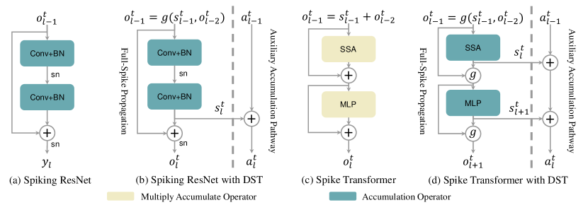
Figure 1: Residual blocks and Dual-stream blocks in Spiking ResNet (Fang et al., 2021a) and Spike Transformer (Zhou et al., 2023). (a) the Spiking ResNet by replacing ReLU activation layers with spiking neurons. (b) The Spiking ResNet with Dual-stream training. (c) The input of the Spike Transformer with Spiking Self-Attention (SSA) is non-spike data due to residual addition between blocks, which brings additional multiply accumulative computation to SNN. (d) Spike Transformer with a dual-stream structure is divided into a spike propagation pathway and a plug-and-play auxiliary accumulation pathway (AAP), which could compensate for full spike propagation. Note AAP could be either retained or removed in model inference.

2 Related Work

2.1 Spiking Neural Networks

To train deep SNNs, ANN to SNN conversion (ANN2SNN) (Hunsberger & Eliasmith, 2015; Cao et al., 2015; Rueckauer et al., 2017; Sengupta et al., 2019; Han et al., 2020; Han & Roy, 2020; Deng & Gu, 2021; Stöckl & Maass, 2021; Li et al., 2021) and backpropagation with surrogate gradient  (Neftci et al., 2019) are the two mainstream methods. For ANN2SNN, an ANN with ReLU activation is first trained, then converts the ANN to an SNN by replacing ReLU with spiking neurons and adding scaling operations like weight normalization and threshold balancing. Recently, several ANN2SNN methods (Han et al., 2020; Han & Roy, 2020; Deng & Gu, 2021; Li et al., 2021) have achieved near loss-less accuracy for VGG-16 and ResNet. However, the converted SNN needs longer time steps to rival the original ANN, and increases the SNN’s computational consumption  (Rueckauer et al., 2017). One of the backpropagation methods (Kim et al., 2020) computes the gradients of the timings of existing spikes with respect to the membrane potential at the spike timing (Comsa et al., 2020; Mostafa, 2017; Kheradpisheh & Masquelier, 2020; Zhou et al., 2021; Zhang & Li, 2020). Another kind of backpropagation method gets the gradient by unfolding the network over the simulation time-steps (Lee et al., 2016; Huh & Sejnowski, 2018; Wu et al., 2018; Shrestha & Orchard, 2018; Lee et al., 2020; Neftci et al., 2019). As the gradient with respect to the threshold-triggered firing is non-differentiable, the surrogate gradient is often used.

2.2 Spiking Residual Networks

For ANN2SNN with ResNet, several methods made specific normalizations for conversion. The residual structure in ANN2SNN with scaled shortcuts is applied in SNN to match the activations of the original ResNet (Hu et al., 2018a). Previous ANN2SNN methods noticed the distinction between plain feedforward ANNs and residual ANNs, and made specific normalizations for conversion. Then, Spike-Norm (Sengupta et al., 2019) is proposed to balance the threshold of the Spiking Neural Model and verified their method by converting ResNet to SNNs. Moreover, existing backpropagation-based methods use nearly the same structure as ResNet. Several custom surrogate methods (Sengupta et al., 2019) are evaluated on shallow ResNets. Threshold-dependent batch normalization (td-BN) is proposed to replace naive batch normalization (BN) (Ioffe & Szegedy, 2015) and successfully trained Spiking ResNet-34/50 directly with surrogate gradient by adding td-BN in shortcuts. SEW ResNet is the first method to increase the SNNs to more than 100 layers, but its use of additive operations in residual connections leads to a none-spike structure in the deep layer of the network bringing higher computational consumption. (Deng et al., 2022) introduces the temporal efficient training approach to compensate for the loss of momentum in the gradient descent with SG so that the training process can converge into flatter minima with better generalizability. (Xiao et al., 2022) proposes online training through time for SNNs, which enables forward-in-time learning by tracking presynaptic activities and leveraging instantaneous loss and gradients. Recently, (Zhou et al., 2023) considers leveraging both self-attention capability and biological properties of SNNs and proposes the Spiking Transformer (Spikformer).

3 Preliminaries

3.1 Spiking Neuron Model

The spiking neuron is the fundamental computing unit of SNNs. The dynamics of all kinds of spiking neurons can be described as follow:

$$H_{t} =SN(V_{t-1},X_{t}),$$ (1)

$$S_{t} =\Theta(H_{t}-V_{th}),$$ (2)

$$V_{t} =H_{t}~{}\left(1-S_{t}\right)+V_{reset}~{}S_{t},$$ (3)

where $X_{t}$ is the input at time-step $t$, $H_{t}$ and $V_{t}$ denote the membrane potential after neuronal dynamics and after the trigger of a spike at time-step $t$, respectively. $V_{th}$ is the firing threshold, $\Theta(x)$ is the Heaviside step function and is defined by $\Theta(x)=1$ for $x\geq 0$ and $\Theta(x)=0$ for $x<0$. $S_{t}$ is the output spike at time-step $t$, which equals 1 if there is a spike and 0 otherwise. $V_{reset}$ denotes the reset potential. The function $SN(\cdot)$ in Eq. (1) describes the neuronal dynamics and takes different forms for different spiking neuron models, which include the Integrate-and-Fire (IF) model (Eq. (4)) and Leaky Integrate-and-Fire (LIF) model (Eq. (5)):

$$H_{t} =V_{t-1}+X_{t},$$ (4)

$$H_{t} =V_{t-1}+\frac{1}{\tau}(X_{t}-(V_{t-1}-V_{reset})),$$ (5)

where $\tau$ represents the membrane time constant. Eq. (2) and Eq. (3) describe the spike generation and resetting processes, which are the same for all kinds of spiking neuron models.

3.2 Computational Consumption

With the sparsity of firing and the short simulation period, SNN can achieve the calculation with about the same number of synaptic operations (SyOPs) (Rueckauer et al., 2017) rather than FLOPs, The number of synaptic operations per layer of the network can be easily estimated for an ANN from the architecture of the convolutional and linear layers. For the ANN, a multiply-accumulate (MAC) computation takes place per synaptic operation. On the other hand, specialized SNN hardware would perform an accumulated computation (AC) per synaptic operation only upon the receipt of an incoming spike. Hence, the total number of AC operations occurring in the SNN would be represented by the dot-product of the average cumulative neural spike count for a particular layer and the corresponding number of synaptic operations. With the deepening of SNN and ANN, the relative energy ratio gradually approaches a fixed value, which could be calculated as follows:

$$\frac{E(\mathrm{SNN})}{E(\mathrm{ANN})}\thickapprox T\cdot fr\cdot\frac{E_{ac}}{E_{mac}},$$ (6)

where $T$ and $fr$ represent the simulation time and the average firing rate.

Eq. (6) assumes the SNN only contains $\{0,1\}$ spike AC operators. However, several SOTA SNNs employ many non-spike MAC and their computation consumption could not be estimated by Eq. (6) accurately. To estimate the computation consumption of different SNNs more accurately, we calculate the number of computations required in terms of AC and MAC synaptic operations, respectively. The main energy consumption of non-spike signals comes from the MAC between neurons. The contribution from one neuron to another requires a MAC for each timestep, multiplying each non-spike activation with the respective weight before adding it to the internal sum. In contrast, a transmitted spike requires only an accumulation at the target neuron, adding weight to the potential, and where spikes may be quite sparse. Therefore, for any SNN network $\mathcal{F}$, the theoretical computational consumption can be determined by the number of AC and MAC operations ($O_{ac},O_{mac}$):

$$\mathrm{E}(\mathcal{F}) =T\cdot(fr\cdot E_{ac}\cdot O_{ac}+E_{mac}\cdot O_{mac}).$$ (7)

Moreover, we developed and open-sourced a tool to calculate the dynamic consumption of SNNs as syops-counter, which can compute the theoretical amount of AC and MAC operations.

3.3 Spiking Residual Blocks

There are two main types of residual blocks for existing SNNs. The one replaces ReLU activation layers with spiking neurons, which constructs FSNN but is prone to vanishing gradient problems. The second uses the same addition operation as the ANN, but leads to additional computation consumption due to the appearance of non-spike signals.

Vanishing Gradient Problems of Spiking ResNet.

Consider a Spiking ResNet with $k$ sequential blocks to transmit $s_{l}^{t}$, and the identity mapping condition is met by using the IF neurons for residual connection with $0<V_{th}\leq 1$, then we have $s_{l}^{t}=s_{l+1}^{t}=...=s_{l+k-1}^{t}=o_{l+k-1}^{t}$. The gradient of the output of the $(l+k-1)$-th residual block with respect to the input of the $l$-th residual block could be calculated layer by layer:

$$\frac{\partial o_{l+k-1}^{t}}{\partial s_{l}^{t}} =\prod_{i=0}^{k-1}\frac{\partial o_{l+i}^{t}}{\partial s_{l+i}^{t}}=\prod_{i=0}^{k-1}\Theta^{\prime}(s_{l+i}^{t}-V_{th})$$ (8)

$$\to\begin{cases}0,\text{if}~{}0<\Theta^{\prime}(s_{l}^{t}-V_{th})<1\\ 1,\text{if}~{}\Theta^{\prime}(s_{l}^{t}-V_{th})=1\\ \end{cases},$$

where $\Theta(x)$ is the Heaviside step function and $\Theta^{\prime}(x)$ is defined by the surrogate gradient. The second equality hold as $o_{l+i}^{t}={\rm SN}(s_{l+i}^{t})$. In view of the fact that $s_{l}^{t}$ could only take $0$ or $1$ with identity mapping, $\Theta^{\prime}(s_{l}^{t}-V_{th})=1$ is not satisfied for commonly used surrogate functions mentioned in (Neftci et al., 2019). When using the common $Sigmoid$ (Neftci et al., 2019) function as the Heaviside step function, the gradient vanishing problem would be prone be happen.

Spiking Residual Blocks with ADD.

As illustrated in Figure 1(c), the residual block for SNN can be formulated with an ADD function (Fang et al., 2021a; Zhou et al., 2023), which can implement identity mapping and overcome the vanishing and exploding gradient problems.

$$o_{l}^{t}=\mathrm{SN}(f_{l}(o_{l-1}^{t}))+o_{l-1}^{t}=s_{l}^{t}+o_{l-1}^{t},$$ (9)

where $s_{l}^{t}$ denotes the residual mapping learned as $s_{l}^{t}=\mathrm{SN}(f_{l}(o_{l-1}^{t}))$. While this design brings performance improvements, it inevitably brings in non-spike data and thus MAC operations. In particular, for the ADD function, if both $s_{l}^{t}$ and $o_{l-1}^{t}$ are spike signals, its output $o_{l}^{t}$ will be a non-spike signal whose value range is $\{0,1,2\}$. As the depth of the network increases, the range of signals transmitted to the next layer of the network will also expand. Convolution requires much more computational overhead of multiplication and addition when dealing with these non-spiking signals as shown in Figure 1(b). In this case, the network will incur additional high computational consumption.

4 Dual-stream Training

4.1 Dual-stream SNN

Basic Block.

Instead of the residual Block containing only one path with respect to the input spike $x$, we initialize the input to two consistent paths $s_{0}^{t}=a_{0}^{t}=x$, where $s_{l}^{t}$ represents the spike signal propagated between blocks, and $a_{l}^{t}$ represents the spike accumulation carried out on the output of each block. As illustrated in Figure 1(b) and (d), the Dual-stream Block can be formulated as:

$$o_{l}^{t} =\begin{cases}\mathrm{SN}(f_{l}(o_{l-1}^{t})+o_{l-1}^{t})=SN(s_{l}^{t}+o_{l-1}^{t})\\ g(\mathrm{SN}(f_{l}(o_{l-1}^{t})),o_{l-1}^{t})=g(s_{l}^{t},o_{l-1}^{t})\\ \end{cases}$$ (10)

$$a_{l}^{t} =s_{l}^{t}+a_{l-1}^{t},$$ (11)

where $g$ represents an element-wise function with two spikes tensors as inputs. Note that here we restrict $g$ to be only the corresponding logical operation function as shown in Table 1, so as to ensure that the input and output of $g$ function are spike trains. Here, Eq.(10) is the full-spike propagation pathway, which could be either of two types of spiking ResNet. Eq.(11) denotes the plug-and-play Auxiliary Accumulation Pathway (AAP). During the inference phase, the auxiliary accumulation could be removed as needed.

Downsampling Block.

Remarkably, when the input and output of one block have different dimensions, the shortcut is set as convolutional layers with stride $>1$, rather than the identity connection, to perform downsampling. The Spiking ResNet utilize {Conv-BN} without ReLU in the shortcut. SEW ResNet (Fang et al., 2021a) adds an SN in shortcut as shown in Figure 2(b). Figure 2(b) shows the downsampling of auxiliary accumulation, that the overhead of multiply accumulation in Dual-stream Blocks mainly comes from the downsampling of the spike accumulation signal. Fortunately, the number of downsampling in a network is always fixed, so the MAC-based downsampling operation of the spike accumulation pathway will not increase with the increase of network depth. Therefore, the increased computational overhead of DSNN with the increase of network depth mainly comes from the accumulation calculation.

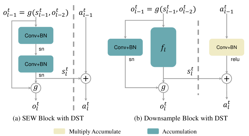
Figure 2: The SEW Block (Fang et al., 2021a) and its Downsample blocks with a dual-stream structure.

Training. For backpropagation, the gradient could be backpropagated to these spiking neurons through the auxiliary accumulation to prevent the vanishing gradient caused by deeper layers. Therefore, in the training phase, the outputs of both auxiliary accumulation and spike propagation are used as the final output and the gradient is calculated according to a consistent objective function $\mathcal{L}_{c}$:

$$\mathcal{L}(x,y)=\mathcal{L}_{c}(\mathcal{O}_{s},y)+\mathcal{L}_{c}(\mathcal{O}_{a},y),$$ (12)

where $\mathcal{O}_{s}$ and $\mathcal{O}_{a}$ are the final outputs of auxiliary accumulation and spike propagation respectively.

4.2 Identity Mapping

As stated in (He et al., 2016b), satisfying identity mapping is crucial to training a deep network.

Auxiliary Accumulation Pathway.

For auxiliary accumulation of Eq.(11), identity mapping is achieved by when $s_{l}^{t}\equiv 0$, which can be implemented by setting the weights and the bias of the last BN layer in $f_{l}$ to zero.

The Spiking Neurons Residuals.

The first spike propagation of Eq.(10) based on Spiking ResNet could implement identity mapping by partial spiking neurons. When $f_{l}(o_{l}^{t-1})\equiv 0$, $o_{l}^{t}={\rm SN}(o_{l}^{t-1})\neq o_{l}^{t-1}$. To transmit $o_{l}^{t-1}$ and make ${\rm SN}(o_{l}^{t-1})=o_{l}^{t-1}$, the last spiking neuron (SN) in the $l$-th residual block needs to fire a spike after receiving a spike and keep silent after receiving no spike at time-step $t$. It works for IF neurons described by Eq. (4). Specifically, we can set $0<V_{th}\leq 1$ and $V_{t-1}=0$ to ensure that $o_{t}=1$ leads to $H_{t}\geq V_{th}$, and $o_{t}=0$ leads to $H_{t}<V_{th}$. Hence, we replaced all the spiking neurons at the residual connections with IF neurons.

Table 1: List of element-wise functions $g$.

Operator $g(x_{l}^{t},s_{l}^{t})$ $\mathrm{AND}$ $s_{l}^{t}\land x_{l}^{t}$ = $s_{l}^{t}\cdot x_{l}^{t}$ $\mathrm{IAND}$ $(\neg s_{l}^{t})\land x_{l}^{t}$ = $(1-s_{l}^{t})\cdot x_{l}^{t}$ $\mathrm{OR}$ $s_{l}^{t}\lor x_{l}^{t}$ = $s_{l}^{t}+x_{l}^{t}-(s_{l}^{t}\cdot x_{l}^{t})$ $\mathrm{XOR}$ $s_{l}^{t}\oplus x_{l}^{t}$ = $s_{l}^{t}\cdot(1-x_{l}^{t})+x_{l}^{t}\cdot(1-s_{l}^{t})$

The Element-wise Logical Residuals.

For the second spike propagation of Eq.(10), different element-wise functions $g$ in Table 1 satisfy identity mapping. Specifically, for $\mathrm{IAND}$, $\mathrm{OR}$ and $\mathrm{XOR}$ as element-wise functions $g$, identity mapping could be achieved by setting $s_{l}^{t}\equiv 0$. Then $o_{l}^{t}=g(s_{l}^{t},o_{l-1}^{t})=g({\rm SN}(0),o_{l-1}^{t})=g(0,o_{l-1}^{t})=o_{l-1}^{t}$. This is consistent with the conditions for auxiliary accumulation Eq.(11) to achieve identity mapping and is applicable to all neuron models. In contrast, for $\mathrm{AND}$ as the element-wise function $g$, $s_{l}^{t}$ should be ones to get identity mapping. Then $o_{l}^{t}=1\land o_{l-1}^{t}=o_{l-1}^{t}$. Although the input parameters of spiking neuron models can be adjusted to practice identity mapping, it is conflicted with the auxiliary accumulation pathway for identity mapping. This is not conducive to maintaining the consistency of signal propagation between the two pathways, thus affecting the effects of training and final recognition. Meanwhile, it is hard to control some spiking neuron models with complex neuronal dynamics to generate spikes at a specified time step.

4.3 Vanishing Gradient Problem

Auxiliary Accumulation Pathway.

The gradient for the auxiliary accumulation pathway is calculated as $\frac{\partial a_{l+k-1}^{t}}{\partial a_{l}^{t}}=\frac{\partial a_{l}^{t}}{\partial a_{l}^{t}}=1$ with identity mapping. Since the above gradient is a constant, the auxiliary accumulation path of Eq. (11) could also overcome the vanishing gradient problems.

The Spiking Neurons Residuals.

Moreover, consider a Spiking ResNet with AAP, the gradient of the output of the $(l+k-1)$-th residual block with respect to the input of the $l$-th residual block with identity mapping could be calculated:

$$\frac{\partial o_{l+k-1}^{t}}{\partial s_{l}^{t}} +\frac{\partial a_{l+k-1}^{t}}{\partial a_{l}^{t}}=\prod_{i=0}^{k-1}\frac{\partial o_{l+i}^{t}}{\partial s_{l+i}^{t}}+\frac{\partial a_{l}^{t}}{\partial a_{l}^{t}}$$ (13)

$$=\prod_{i=0}^{k-1}\Theta^{\prime}(s_{l+i}^{t}-V_{th})+\frac{\partial a_{l}^{t}}{\partial a_{l}^{t}}$$

$$\to\begin{cases}1,\text{if}~{}0<\Theta^{\prime}(s_{l}^{t}-V_{th})<1\\ 2,\text{if}~{}\Theta^{\prime}(s_{l}^{t}-V_{th})=1\\ \end{cases},$$

Since the above gradient is a constant, the Spiking ResNet with AAP could alleviate the vanishing gradient problems.

The Element-wise Logical Residuals.

When the identity mapping is implemented for the spiking propagation path of Eq.(10), the gradient of the output of the $(l+k)$-th dual-stream block with respect to the input of the $l$-th DSNN block could be calculated layer by layer:

$$\frac{\partial o_{l+k-1}^{t}}{\partial x_{l}^{t}} =\prod_{i=0}^{k}\frac{\partial g(s_{l+i}^{t},x_{l+i}^{t})}{\partial x_{l+i}^{t}}$$ (14)

$$=\begin{cases}\prod_{i=0}^{k}\frac{\partial(1\cdot x_{l+i}^{t})}{\partial x_{l+i}^{t}},\text{if}~{}~{}g=\mathrm{AND}\\ \prod_{i=0}^{k}\frac{\partial((1-0)\cdot x_{l+i}^{t})}{\partial x_{l+i}^{t}},\text{if}~{}~{}g=\mathrm{IAND}\\ \prod_{i=0}^{k}\frac{\partial((1+0-0)\cdot x_{l+i}^{t})}{\partial x_{l+i}^{t}},\text{if}~{}~{}g=\mathrm{OR}\\ \prod_{i=0}^{k}\frac{\partial((1+0)\cdot x_{l+i}^{t})}{\partial x_{l+i}^{t}},\text{if}~{}~{}g=\mathrm{XOR}\end{cases}=1.$$

The second equality holds as identity mapping is achieved by setting $s_{l+i}^{t}\equiv 1$ for $g=\mathrm{AND}$, and $s_{l+i}^{t}\equiv 0$ for $g=\mathrm{IAND/OR/XOR}$. Since the gradient in Eq. (14) is a constant, the spiking propagation path of Eq.(10) overcomes the vanishing gradient problems.

5 Experiments

5.1 Computational Consumption

To estimate the computational consumption of different SNNs, we calculate the number of computations required in terms of AC and MAC synaptic operations, respectively. Moreover, (Rueckauer et al., 2017) integrates batch normalization (BN) layers into the weights of the preceding layer with loss-less conversion. Therefore, we ignore BN operations when calculating the number of MAC operations, resulting in a more efficient inference consumption. See Appendix A for details of the fusion process of convolution with BN. To quantitatively estimate energy consumption, we evaluate the computational consumption based on the number of AC and MAC operations and the data for various operations in $45nm$ technology (Horowitz, 2014), where $\mathrm{E}_{\mathrm{MAC}}$ and $\mathrm{E}_{\mathrm{AC}}$ are $4.6pJ$ and $0.9pJ$ respectively. Here, we calculate the Dynamic Consumption (DC) of the SNN by Eq.(8) based on its spike firing rate on the target dataset. Moreover, we use the Estimated Consumption (EC) to estimate the theoretical consumption range from $[0,100\%]$ spike firing rate, that is

$$\mathrm{E}(\mathcal{F})\in[T\cdot E_{mac}\cdot O_{mac},T\cdot(E_{ac}\cdot O_{ac}+E_{mac}\cdot O_{mac})].$$ (15)

5.2 ImageNet Classification

We validate the effectiveness of our Dual-stream Training method on image classification of ImageNet (Deng et al., 2009) dataset. The IF neuron model is adopted for the static ImageNet dataset. For a fair comparison, all of our training parameters are consistent with SEW ResNet (Fang et al., 2021a). As shown in Table 2, two variations of our DST are evaluated: “FSNN (DST)” means the FSNN is trained by the proposed DST and AAP is removed in the test phase, and “DSNN” means the APP is retained to improve the discrimination of features. “FSNN-18” and ”DSNN-18” represents the SNN is designed based on ResNet-18, and so on. Three types of methods are compared respectively: “A2S” represents ANN2SNN methods, “FSNN” and “MPSNN” means Full Spike Neural Networks and Mixed-Precision Spike Neural Networks respectively. These notations keep the same in the below.

Table 2: Comparison with previous Spiking ResNet on ImageNet. $\dagger$ denotes the estimated dynamic consumption based on the spike firing rate provided in the corresponding paper. A2S represents ANN2SNN methods, FSNN and MPSNN mean Full Spike Neural Networks and Mixed-Precision Spike Neural Networks respectively. FSNN (DST) represent the FSNN is trained by the proposed DST and DSNN means APP is retained in the test phase.

Network Methods Acc@1 $T$ EC(mJ) $O_{ac}$(G) $O_{mac}$(G) DC(mJ) PreAct-ResNet-18 (Meng et al., 2022) A2S 67.74 50 $[1.43,77.84]$ - - - Spiking ResNet-34 (Rathi et al., 2020) A2S 61.48 250 $[7.31,805.79]$ - - - Spiking ResNet-34 (Li et al., 2021) A2S 74.61 256 $[7.45,825.29]$ - - - Spiking ResNet-34 with td-BN (Zheng et al., 2021) FSNN 63.72 6 $[0.69,19.85]$ 5.34 0.15 5.50 ^† Spiking ResNet-50 with td-BN (Zheng et al., 2021) FSNN 64.88 6 $[1.10,22.59]$ 6.01 0.24 6.52 ^† Spiking ResNet-34 (Deng et al., 2022) FSNN 64.79 6 $[0.69,19.85]$ 5.34 0.15 5.50 ^† FSNN-18 (DST) FSNN 62.16 4 $[0.55,4.31]$ 1.69 0.12 2.07 FSNN-34 (DST) FSNN 66.45 4 $[0.55,7.64]$ 3.42 0.12 3.63 FSNN-50 (DST) FSNN 67.69 4 $[0.55,10.42]$ 3.14 0.12 3.38 FSNN-101 (DST) FSNN 68.38 4 $[0.55,20.64]$ 4.42 0.12 4.53 SEW ResNet-18 (ADD) (Fang et al., 2021a) MPSNN 63.18 4 $[12.65,16.40]$ 0.51 2.75 13.11 SEW ResNet-34 (ADD) (Fang et al., 2021a) MPSNN 67.04 4 $[29.72,36.78]$ 0.86 6.46 30.50 SEW ResNet-50 (ADD) (Fang et al., 2021a) MPSNN 67.78 4 $[23.64,33.50]$ 2.01 5.14 25.45 SEW-ResNet-34 (ADD) (Deng et al., 2022) MPSNN 68.00 4 $[29.72,36.78]$ 0.86 6.46 30.50 ^† SEW ResNet-101 (ADD) (Fang et al., 2021a) MPSNN 68.76 4 $[39.88,59.97]$ 3.07 8.67 42.65 DSNN-18 MPSNN 63.46 4 $[0.92,4.67]$ 1.69 0.20 2.44 DSNN-34 MPSNN 67.52 4 $[0.92,8.00]$ 3.42 0.20 4.00 DSNN-50 MPSNN 69.56 4 $[6.30,16.17]$ 3.20 1.37 9.18 DSNN-101 MPSNN 71.12 4 $[6.30,26.39]$ 4.48 1.37 10.33

As shown in Table 2, we can obtain 3 following key findings:

First, the SOTA ANN2SNN methods (Li et al., 2021; Hu et al., 2018b) achieve higher accuracies than FSNN as well as other SNNs trained from scratch, but they use 64 and 87.5 times as many time-steps as FSNN respectively, which means that they require more computational consumption. Since most of these methods do not provide the trained models and their DCs are not available, we only used EC to evaluate the consumption. From Table 2, these models with larger time steps also have larger computational consumption. (Meng et al., 2022) also achieves good performance with ResNet-18, but its SNN acquisition process is relatively complex. It needs ANN to pre-train the model first and then retrain the SNN. Although its time steps are less than other ANN2SNN methods, it is still 12.5 times that of DSNN. Due to ANN2SNN being a different type of method from ours, the comparisons are listed just for reference.

Second, for full-spike neural networks, FSNN (DST) outperforms Spiking ResNet (Zheng et al., 2021; Deng et al., 2022) even with lower computational consumption. The performance of FSNN (DST) has a major advantage over other FSNNs and also improves with the increasing depth of the network. It indicates that the proposed DST is indeed helpful to train FSNN.

Finally, the performance of DSNN is further improved when AAP is added to FSNN at the inference phase. At the same time, the DSNN offers superior performance compared to the mixed-precision SEW ResNet (Fang et al., 2021a). Note that the performance gap between SEW ResNet-34 and SEW ResNet-50 is not big, and the computational consumption of SEW ResNet-34 is higher than SEW ResNet-50. This phenomenon comes from that ResNet-34 and ResNet-50 use BasicBlock (He et al., 2016a) and Bottleneck (He et al., 2016a) as blocks respectively. As shown in Figure 1 (b), the first-layer convolution of each block is regarded as a MAC computation operation due to the non-spike data generated by ADD function. However, the first-layer convolution of BasicBlock is much larger than the synaptic operation of Bottleneck, which causes the computational consumption of SEW ResNet-34 to be greater than that of ResNet-50. In contrast, DSNN ensures that the input and output of each block are spike data through the dual-stream mechanism, so that the theoretical computational consumption increases linearly with the increase of network depth.

5.3 DVS Classification

DVS Gesture.

We also compare our method with SEW ResNet-7B-Net (Fang et al., 2021a) on the DVS Gesture dataset (Amir et al., 2017), which contains 11 hand gestures from 29 subjects under 3 illumination conditions. We use the similar network structure 7B-Net in (Fang et al., 2021a). As shown in Table 3, FSNN-7 (DST) with $\mathrm{IAND}$ obtains better performance than other FSNN methods, such as SEW with $\mathrm{IAND}$ and td-BN, demonstrating the DST is effective to train FSNN. In addition, even though SEW utilizes $\mathrm{IAND}$ as $g(\cdot)$ which brings non-spike operations, our FSNN-7 (DST) still achieves comparable performance, and only requires a tenth of the computational consumption of SEW.

CIFAR10-DVS.

We also evaluate Spiking ResNet models on the CIFAR10-DVS dataset (Li et al., 2017), which is obtained by recording the moving images of the CIFAR-10 dataset on an LCD monitor by a DVS camera. We use Wide-7B-DSNN which is a similar network structure Wide-7B-Net in (Fang et al., 2021a). As shown in Table 3, FSNN-7 (DST) achieves better performance and lower computational consumption than the previous Spiking ResNet (Zheng et al., 2021) and SEW ResNet (Fang et al., 2021a).

Table 3: Comparison with Spiking ResNet methods on DVS Gesture and CIFAR10-DVS. Once the ADD function is used as $g(\cdot)$, it will bring non-spiking operation to SEW (Fang et al., 2021a). The comparison with it is listed just for reference.

Networks $g(\cdot)$ DVS Gesture CIFAR10-DVS $T$ ACC/DC(mJ) SEW (Fang et al., 2021a) $\mathrm{ADD}$ 97.92/17.09 74.4/16.71 16 SEW (Fang et al., 2021a) $\mathrm{IAND}$ 95.49/1.48 - 16 td-BN (Zheng et al., 2021) - 96.87/- 67.8/- 40/10 FSNN-7 (DST) $\mathrm{AND}$ 55.56/2.59 70.9/3.57 16 FSNN-7 (DST) $\mathrm{OR}$ 96.18/1.04 74.8/3.51 16 FSNN-7 (DST) $\mathrm{XOR}$ 96.53/1.19 74.0/3.41 16 FSNN-7 (DST) $\mathrm{IAND}$ 97.57/1.10 73.1/4.65 16

5.4 Further Analysis

Computational Consumption

Here, we analyze the computational consumption advantages of DSNN. First, the networks in most ANN2SNN methods are full-spike, where few MAC operations are from batch normalization and conversion of images to spikes. However, their computational consumption is still very large due to the large time steps. DSNN and FSNN has fewer time steps than ANN2SNN methods, which means that its theoretical maximum consumption is much smaller than ANN2SNN as shown in Table 2. Second, the DSNN has lower EC and DC than Spiking ResNet based on addition (SEW ResNet), and achieves better performance. The additive-based SEW ResNet will increase its AC and MAC as the network gets deeper, which will bring about a multifold increase in computational consumption. In contrast, the main MAC operation for DSNN comes from the downsampling process of accumulated signals in spike accumulation. Therefore, a deeper DSNN only increases the AC operation, and its MAC operation is constant as shown in Table 2. Finally, it also reveals for the first time the positive relationship between computational consumption and the performance of SNNs. In addition, the performance of DSNN increases gradually with the increase in computational consumption. It indicates the added computational consumption of deeper DSNN is meaningful.

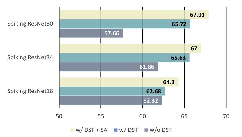
Figure 3: Training Spiking ResNet from scratch on ImageNet with/without Dual-Stream Training.

Vanishing Gradient Problem.

As mentioned in Section 3.3, Spiking ResNet suffers from a vanishing gradient problem. As shown in Figure 3, the performance of the Spiking ResNet gradually decreases as the number of network layers increases. Network depth did not bring additional gain to the original Spiking ResNet. With the addition of DST, the performance of the Spiking ResNet gradually increases with increasing network depth. Also, the performance is superior with the addition of AAP. As demonstrated in Eq.(13), DST could help alleviate the vanishing gradient problem of the Spiking ResNet.

Feature Enhancement.

Here, we analyze the effects of auxiliary accumulation in terms of improving feature discrimination. Moreover, AAP increases the feature discriminant of forward as shown in Figure 4. Under fewer time steps, the spike feature is almost a binary feature, because its discrete property limits the discriminant of its feature. The discrimination of features from spike propagation is not enough, which affects the overall performance. On the other hand, we could increase the number of deep spike features by increasing time steps, so as to improve the discrimination by increasing the number of features, which often leads to too high computational consumption as shown in Table 2. More importantly, AAP separates the computation of AC operations from the MAC computation of recognition, allowing SNN to take full advantage of its low computational consumption.

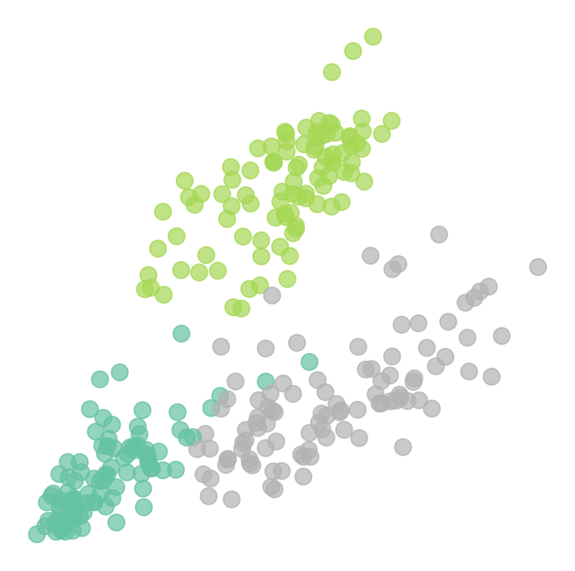
(a) FSNN (DST)

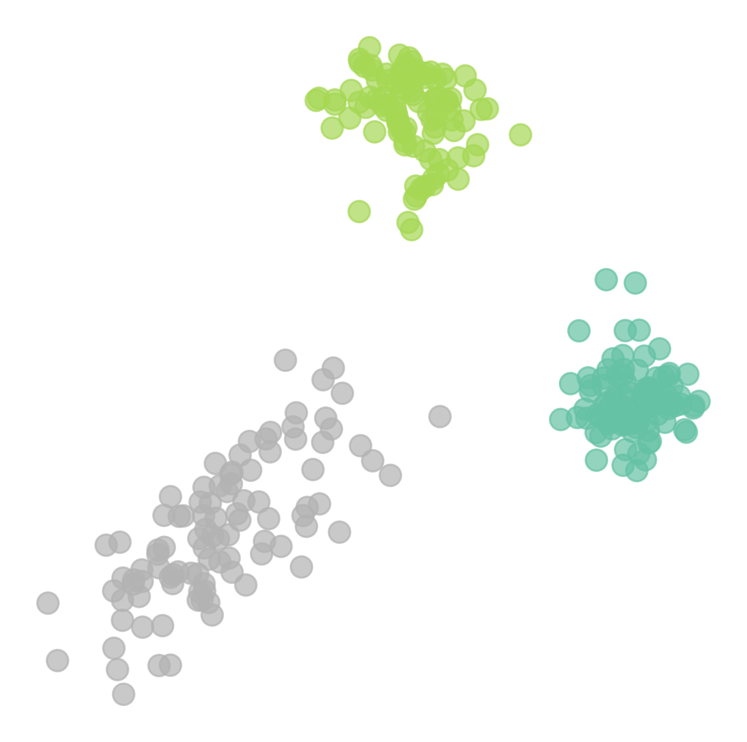
(b) DSNN

Figure 4: The the t-SNE (Maaten & Hinton, 2008) plots of embedding features on DVS Gesture.

Spike Transformer.

We also test the role of DST on the Transformer on CIFAR100. The latest method Spikeformer (Zhou et al., 2023) utilizes $\mathrm{ADD}$ as its residual connection and achieve SOTA performance. However, the $\mathrm{ADD}$ introduces additional computational consumption from non-spike data. As shown in Table 4, once the $\mathrm{IAND}$ is replaced by $\mathrm{IAND}$, the performance of the full-spike Spikeformer will drop. After introducing APP as shown in Figure 1, the Spikeformer with a full-spike signal achieves similar performance to the original mixed-precision Spikeformer. Notably, there is no downsampling in the Spikeformer, which further exploits the advantages of AAP while not introducing additional MAC operations. The small amount of MAC operations comes mainly from the image-to-spike conversion and the classifier operations.

Table 4: Learning Spike Transformer (Zhou et al., 2023) with DST. ADD will bring additional computational consumption from non-spike data. Spikformer (IAND) is the full-spike version of Spikformer, and Spikformer (IAND) w/ DST means the full-spike Spikformer is trained by our DST.

Networks Method Acc DC(mJ) Spikformer (ADD) MPSNN 77.21 5.27 Spikformer (IAND) FSNN 75.54 0.82 Spikformer (IAND) w/ DST FSNN 76.96 0.84

6 Conclusion & Outlook

In this paper, we point out that the main contradiction of FSNNs comes from information loss of full spike propagation. Therefore, we propose the Auxiliary Accumulation Pathway with consistent identity mapping which is able to compensate for the loss of information forward and backward from full spike propagation, so as to keep computationally efficient and high-performance recognition simultaneously. The experiments on the ImageNet, DVS Gesture, and CIFAR10-DVS indicate that DST could improve the ResNet-based and Transformer-baed SNNs trained from scratch in both accuracy and computation consumption. Looking forward, this SNN with a dual-stream structure may provide a reference for the design of neuromorphic hardware, which could improve computational efficiency by separating spike and non-spike computation. In addition, the proposed dual-streams mechanism is similar to the dual-streams object recognition pathway in the human brain, which may provide a new potential direction for SNN structure design.

Appendix A The Fusion of $\mathrm{Conv}+\mathrm{BN}$

The fusion of convolution and batch normalization. It should be noted that the spike signal becomes the floating point once it has passed through the convolution layer, which leads to subsequent MAC operations from the Batch Normalization (BN). However, the homogeneity of convolution allows the following BN and linear scaling transformation to be equivalently fused into the convolutional layer with an added bias (Ding et al., 2019, 2021). Specifically, each BN and its preceding convolution layer into a convolution with a bias vector. Let $\{\mathrm{W}^{\prime},\mathrm{B}^{\prime}\}$ be the kernel and bias converted from $\{\mathrm{W},\boldsymbol{\mathbf{\mu}},\boldsymbol{\mathbf{\sigma}},\boldsymbol{\mathbf{\gamma}},\boldsymbol{\mathbf{\beta}}\}$, we have

$$\mathrm{W}^{\prime}=\frac{\boldsymbol{\mathbf{\gamma}}_{i}}{\boldsymbol{\mathbf{\sigma}}_{i}}\mathrm{W}\,,\quad\mathrm{B}^{\prime}_{i}=-\frac{\boldsymbol{\mathbf{\mu}}_{i}\boldsymbol{\mathbf{\gamma}}_{i}}{\boldsymbol{\mathbf{\sigma}}_{i}}+\boldsymbol{\mathbf{\beta}}_{i}\,.$$ (16)

Then it is easy to verify that,

$$\text{bn}(\mathrm{M}\ast\mathrm{W},\boldsymbol{\mathbf{\mu}},\boldsymbol{\mathbf{\sigma}},\boldsymbol{\mathbf{\gamma}},\boldsymbol{\mathbf{\beta}})=(\mathrm{X}\ast\mathrm{W}^{\prime})+\mathrm{B}^{\prime}\,.$$ (17)

Therefore, when calculating the theoretical computational consumption, ignore the consumption of the BN could be ignored.

Appendix B Implementation Details

All experiments are implemented with SpikingJelly (Fang et al., 2022), which is an open-source deep learning framework for SNNs based on PyTorch (Paszke et al., 2019). The source code is included in the supplementary. The hyper-parameters of the DSNN for different datasets are shown in Table 5. The pre-processing data methods for three datasets are as follows:

Table 5: Hyper-parameters of the DSNN for ImageNet, DVS Gesture, and CIFAR10-DVS datasets. CA denotes the Cosine Annealing (Loshchilov & Hutter, 2017).

Dataset Learning Rate Scheduler Epochs $\boldsymbol{lr}$ Batch Size $\boldsymbol{T}$ ImageNet CA, $T_{max}=320$ 320 0.1 128 4 DVS Gesture Step, $T_{step}=64.\gamma=0.1$ 192 0.005 16 16 CIFAR10-DVS CA, $T_{max}=64$ 64 0.01 16 16 CIFAR100 CA 310 $5e-4$ 128 4

ImageNet. The data augmentation methods used in (He et al., 2016a) are also applied in our experiments. A 224×224 crop is randomly sampled from an image or its horizontal flip with data normalization for train samples. A 224×224 resize and central crop with data normalization are applied for test samples.

DVS Gesture. We utilize random temporal delete (Fang et al., 2021a) to relieve overfitting. Denote the sequence length as $T$, we randomly delete $T-T_{train}$ slices in the original sequence and use $T_{train}$ slices during training. During inference we use the whole sequence, that is, $T_{test}=T$. We set $T_{train}=12,T=16$ in all experiments on DVS Gesture.

CIFAR10-DVS. We use the AER data pre-processing in (Fang et al., 2021b) for DVS128 Gesture. We do not use random temporal delete because CIFAR10-DVS is obtained by static images.

CIFAR100. All hyperparameters are consistent with (Zhou et al., 2023).

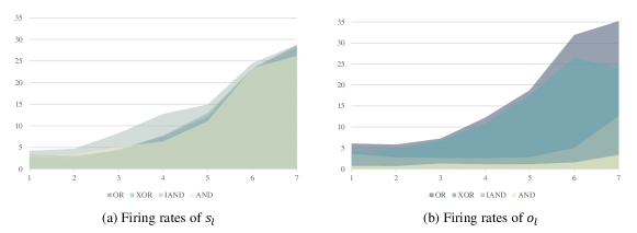
Figure 5: Firing rates of Dual-stream Blocks on DVS Gesture.

Appendix C More Analysis

C.1 Analysis of Spiking Response of Dual-Stream Block

Furthermore, we analyze the firing rates of DSNN, which are closely related to computational power consumption. Figure 5(a) shows the firing rates of $o_{l}$ for the Dual-Stream Block on DVS Gesture, where all spiking neurons in dual-stream blocks have low firing rates, and the spiking neurons in the first two blocks even have firing rates of almost zero. All firing rates in the dual-stream blocks are not larger than 0.5, indicating that all neurons fire on average not more than two spikes. The firing rates of $o_{l}$ in the first few blocks are at a low level, verifying that most dual-stream blocks act as identity mapping. As the depth of the network accelerates, the fire rate increases, increasing the ability to express features for better recognition.

C.2 Evaluation of Different Element-wise Functions

We evaluate all kinds of element-wise functions $g$ on CIFAR10-DVS and DVS Gesture as shown in Table 3. As mentioned above, both pathways of DSNN should achieve identity mapping under the same conditions, and $\mathrm{IAND}$, $\mathrm{OR}$, and $\mathrm{XOR}$ (except $\mathrm{AND}$) satisfy this. As shown in Table 3, the performance of $\mathrm{AND}$ is lower than other functions as expected. It also indicates the necessity of identity mapping. Moreover, $\mathrm{IAND}$, $\mathrm{OR}$, and $\mathrm{XOR}$ all achieved relatively good performance on CIFAR10-DVS and DVS Gesture. On the other hand, Figure 5 shows the fire rates for different element-wise $g(\cdot)$ functions. For different element-wise $g(\cdot)$ functions, the output $s_{l}$ of each block is not obviously different. However, for the fire rate after the element-wise $g(\cdot)$ function, the output $o_{l}$ gap of each block is obvious. As shown in Figure 5(b), $\mathrm{OR}>\mathrm{XOR}>\mathrm{IAND}>\mathrm{AND}$ for the firing rate. For datasets with different complexity, different firing rates can be needed for better recognition. For example, $\mathrm{IAND}$ achieves the best performance for a simple DVS dataset. However, for the slightly complex CIFAR10-DVS, $\mathrm{OR}$ has a higher rate to improve the feature expression ability, thus achieving the best performance.

C.3 Gradients Check on Deeper DSNN

Eq. (11) and Eq. (12) analyze the gradients of multiple blocks with identity mapping. To verify that DSNN can overcome the vanishing/exploding gradient, we check the gradients of the deeper DSNN with 50 layers. In this paper, the surrogate gradient method (Neftci et al., 2019) is used to define $\Theta^{\prime}(x)\triangleq\sigma^{\prime}(x)$ during error back-propagation, with $\sigma(x)$ denote the surrogate function. The surrogate gradient function we used in all experiments is $\sigma(x)=\frac{1}{\pi}\arctan(\frac{\pi}{2}\alpha x)+\frac{1}{2}$, thus $\sigma^{\prime}(x)=\frac{\alpha}{2(1+(\frac{\pi}{2}\alpha x)^{2})}$.

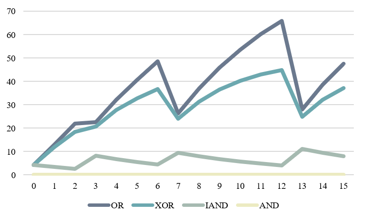
(a) Firing rate of $o_{l}$

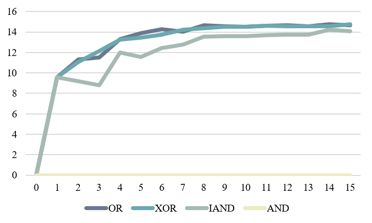
(b) Firing rate of $s_{l}$

Figure 6: The initial firing rates of output $o_{l}$ and $s_{l}$ in $l$-th block on 50 layer network.

Initial Firing Rates

As the gradients of SNNs are significantly influenced by initial firing rates (Fang et al., 2021a), he we analyze the firing rate. Figure 6 shows the initial firing rate of $l$-th block’s output $o_{l}$, where the mutations occur due to downsampling blocks. As shown in Figure 6(a), the silence problem happens in the DSNN with $\mathrm{AND}$ (yellow curve). When using $\mathrm{AND}$, $o_{l}^{t}={\rm SN}(f^{l}(o_{l-1}^{t}))\land o_{l-1}^{t}\leq o_{l-1}^{t}$. Since it is hard to keep ${\rm SN}(f^{l}(o_{l-1}^{t}))=1$ at each time-step $t$, the silence problem may frequently happen in DSNN with $\mathrm{AND}$. In contrast, compared with $\mathrm{AND}$, using $\mathrm{OR}$, $\mathrm{XOR}$ and $\mathrm{IAND}$ could easily maintain a certain firing rate. Figure 6(b) shows the firing rate of $s_{l}={\rm SN}(f^{l}(o_{l-1}^{t}))$, which represents the output of the last SN in $l$-th block. It shows that although the firing rate of $o_{l}$ in DSNN with $\mathrm{OR}$, $\mathrm{XOR}$ and $\mathrm{IAND}$ could increase constantly with the depth of networks in theory, the last SN in each block still maintains a stable firing rate in practice.

Vanishing Gradient

To analysis the vanishing gradient, we set $V_{th}=1$ and $\alpha=2$ in the surrogate function $\sigma(x)$. In this case, $\sigma^{\prime}(x)\leq\sigma^{\prime}(0)=\sigma^{\prime}(1-V_{th})=1$ and $\sigma^{\prime}(0-V_{th})=0.092<1$, and transmitting spikes to SNs is prone to causing vanishing gradient. The gradient amplitude $\left\|\frac{\partial L}{\partial S^{l}}\right\|$ of each block is shown in Figure 7(a-d), and DSNN do not be affected no matter what $g$ we choose.This is caused that in the identity mapping areas, $s_{l}$ is constant for all index $l$, and the gradient also becomes a constant as it will not flow through SNs. Compared with the case where only spike propagation exists (Figure 7(e-h)), the gradient in DSNN is more stable. In addition, DSNN even could significantly improve $\mathrm{AND}$ which would limit the neuron firing and affect the gradient. It indicates the effectiveness of the DSNN for the vanishing gradient.

Exploding Gradient

Similar, here we set $V_{th}=1,\alpha=3$ in the surrogate function $\sigma(x)$ to analysis the exploding gradient, where $\sigma^{\prime}(1-V_{th})=1.5>1$ and transmitting spikes to SNs is prone to causing exploding gradient. As shown in Figure 8 (a-d), exploding gradient problem in DSNN with $\mathrm{OR}$, $\mathrm{XOR}$, $\mathrm{IAND}$, and $\mathrm{AND}$ is not serious. Compared to Spiking ResNet without spike accumulation (Figure 8 (d-h)), DSNN has a more gradual gradient.

Silence Problem of AND

Moreover, some vanishing gradient happens in the Spiking ResNet with $\mathrm{AND}$ as shown in Figure 7(h) and 8(h) (The gradient of $\mathrm{AND}$ is $0$), which is caused by the silence problem. The attenuation of the gradient caused by the silent problem can be alleviated by the backpropagation of the spike accumulation path as shown in igure 7 and 8. The gradients of DSNN with $\mathrm{OR}$, $\mathrm{XOR}$, $\mathrm{IAND}$, and $\mathrm{AND}$ increase slowly when propagating from deeper layers to shallower layers.

In general, DSNN could overcome the vanishing or exploding gradient problem well through spike accumulation. At the same time, spike accumulation accumulates the output spikes of each block, thus increasing the discriminability of the features in network inference.

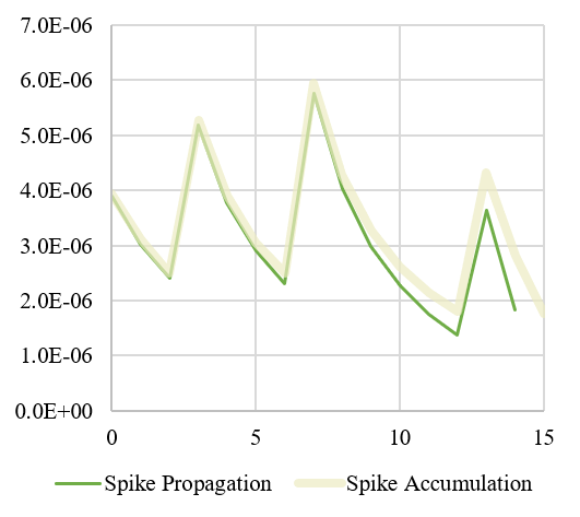
(a) $\mathrm{OR}$

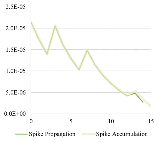
(b) $\mathrm{XOR}$

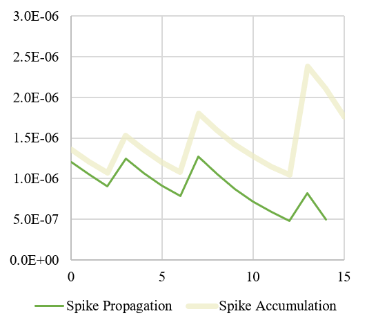
(c) $\mathrm{IAND}$

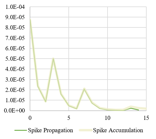
(d) $\mathrm{AND}$

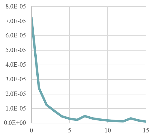
(e) $\mathrm{OR}$ w/o SA

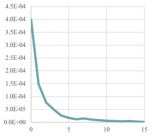
(f) $\mathrm{XOR}$ w/o SA

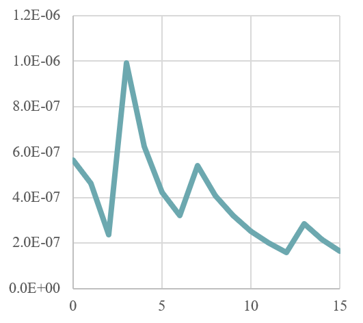
(g) $\mathrm{IAND}$ w/o SA

(h) $\mathrm{AND}$ w/o SA

Figure 7: Gradient amplitude $\left\|\frac{\partial L}{\partial s_{l}}\right\|$ of $l$-th block when $V_{th}=1,\alpha=2$ in the surrogate function $\sigma(x)$.

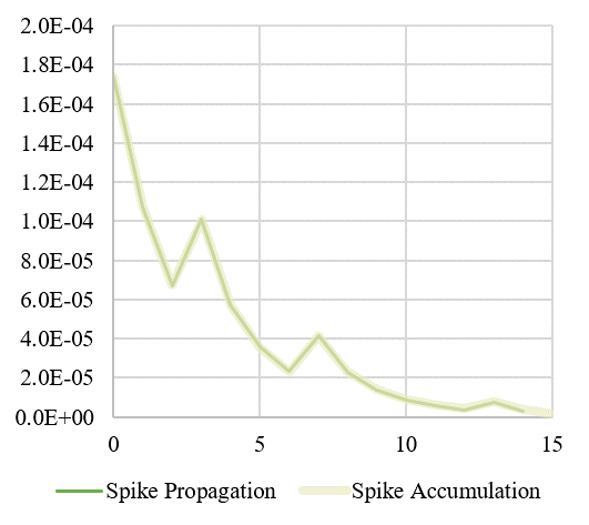
(a) $\mathrm{OR}$

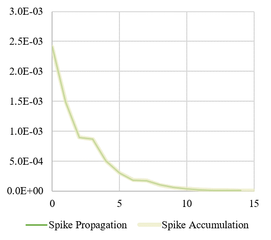
(b) $\mathrm{XOR}$

(c) $\mathrm{IAND}$

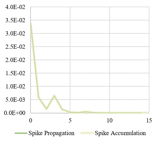
(d) $\mathrm{AND}$

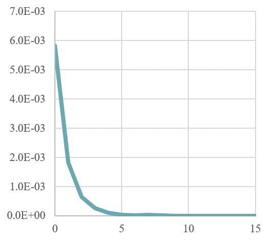
(e) $\mathrm{OR}$ w/o SA

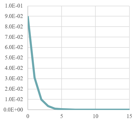
(f) $\mathrm{XOR}$ w/o SA

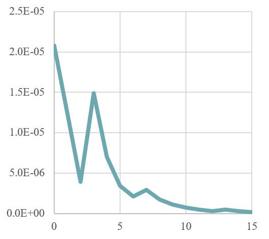
(g) $\mathrm{IAND}$ w/o SA

(h) $\mathrm{AND}$ w/o SA

Figure 8: Gradient amplitude $\left\|\frac{\partial L}{\partial s_{l}}\right\|$ of $l$-th block when $V_{th}=1,\alpha=3$ in the surrogate function $\sigma(x)$.

References

- Amir et al. (2017) Amir, A., Taba, B., Berg, D., Melano, T., McKinstry, J., Di Nolfo, C., Nayak, T., Andreopoulos, A., Garreau, G., Mendoza, M., Kusnitz, J., Debole, M., Esser, S., Delbruck, T., Flickner, M., and Modha, D. A low power, fully event-based gesture recognition system. In Proceedings of the IEEE Conference on Computer Vision and Pattern Recognition (CVPR), pp. 7243–7252, 2017.
- Cao et al. (2015) Cao, Y., Chen, Y., and Khosla, D. Spiking deep convolutional neural networks for energy-efficient object recognition. International Journal of Computer Vision, 113(1):54–66, 2015.
- Chen & Chen (2018) Chen, G. and Chen, Z. Saliency detection by superpixel-based sparse representation. In Advances in Multimedia Information Processing–PCM 2017: 18th Pacific-Rim Conference on Multimedia, Harbin, China, September 28-29, 2017, Revised Selected Papers, Part II 18, pp. 447–456. Springer, 2018.
- Chen et al. (2020) Chen, G., Qiao, L., Shi, Y., Peng, P., Li, J., Huang, T., Pu, S., and Tian, Y. Learning open set network with discriminative reciprocal points. In Computer Vision–ECCV 2020: 16th European Conference, Glasgow, UK, August 23–28, 2020, Proceedings, Part III 16, pp. 507–522. Springer, 2020.
- Chen et al. (2021a) Chen, G., Peng, P., Ma, L., Li, J., Du, L., and Tian, Y. Amplitude-phase recombination: Rethinking robustness of convolutional neural networks in frequency domain. In Proceedings of the IEEE/CVF International Conference on Computer Vision, pp. 458–467, 2021a.
- Chen et al. (2021b) Chen, G., Peng, P., Wang, X., and Tian, Y. Adversarial reciprocal points learning for open set recognition. IEEE transactions on pattern analysis and machine intelligence, 2021b. doi: 10.1109/TPAMI.2021.3106743.
- Comsa et al. (2020) Comsa, I. M., Potempa, K., Versari, L., Fischbacher, T., Gesmundo, A., and Alakuijala, J. Temporal coding in spiking neural networks with alpha synaptic function. In International Conference on Acoustics, Speech and Signal Processing (ICASSP), pp. 8529–8533. IEEE, 2020.
- Deng et al. (2009) Deng, J., Dong, W., Socher, R., Li, L.-J., Li, K., and Fei-Fei, L. Imagenet: A large-scale hierarchical image database. In 2009 IEEE conference on computer vision and pattern recognition, pp. 248–255. Ieee, 2009.
- Deng & Gu (2021) Deng, S. and Gu, S. Optimal conversion of conventional artificial neural networks to spiking neural networks. In International Conference on Learning Representations (ICLR), 2021. URL https://openreview.net/forum?id=FZ1oTwcXchK.
- Deng et al. (2022) Deng, S., Li, Y., Zhang, S., and Gu, S. Temporal efficient training of spiking neural network via gradient re-weighting. In International Conference on Learning Representations, 2022.
- Ding et al. (2019) Ding, X., Guo, Y., Ding, G., and Han, J. Acnet: Strengthening the kernel skeletons for powerful cnn via asymmetric convolution blocks. In Proceedings of the IEEE International Conference on Computer Vision, pp. 1911–1920, 2019.
- Ding et al. (2021) Ding, X., Zhang, X., Ma, N., Han, J., Ding, G., and Sun, J. Repvgg: Making vgg-style convnets great again. In Proceedings of the IEEE/CVF Conference on Computer Vision and Pattern Recognition, pp. 13733–13742, 2021.
- Fang et al. (2021a) Fang, W., Yu, Z., Chen, Y., Huang, T., Masquelier, T., and Tian, Y. Deep residual learning in spiking neural networks. Advances in Neural Information Processing Systems, 34:21056–21069, 2021a.
- Fang et al. (2021b) Fang, W., Yu, Z., Chen, Y., Masquelier, T., Huang, T., and Tian, Y. Incorporating learnable membrane time constant to enhance learning of spiking neural networks. In Proceedings of the IEEE/CVF International Conference on Computer Vision (ICCV), pp. 2661–2671, 2021b.
- Fang et al. (2022) Fang, W., Chen, Y., Ding, J., Chen, D., Yu, Z., Zhou, H., Tian, Y., and other contributors. Spikingjelly. https://github.com/fangwei123456/spikingjelly, 2022.
- Girshick et al. (2014) Girshick, R., Donahue, J., Darrell, T., and Malik, J. Rich feature hierarchies for accurate object detection and semantic segmentation. In Proceedings of the IEEE Conference on Computer Vision and Pattern Recognition (CVPR), pp. 580–587, 2014.
- Han & Roy (2020) Han, B. and Roy, K. Deep spiking neural network: Energy efficiency through time based coding. In European Conference on Computer Vision (ECCV), pp. 388–404, 2020.
- Han et al. (2020) Han, B., Srinivasan, G., and Roy, K. Rmp-snn: Residual membrane potential neuron for enabling deeper high-accuracy and low-latency spiking neural network. In Proceedings of the IEEE/CVF Conference on Computer Vision and Pattern Recognition (CVPR), pp. 13558–13567, 2020.
- He et al. (2016a) He, K., Zhang, X., Ren, S., and Sun, J. Deep residual learning for image recognition. In Proceedings of the IEEE/CVF Conference on Computer Vision and Pattern Recognition (CVPR), pp. 770–778, 2016a.
- He et al. (2016b) He, K., Zhang, X., Ren, S., and Sun, J. Identity mappings in deep residual networks. In European Conference on Computer Vision (ECCV), pp. 630–645. Springer, 2016b.
- Horowitz (2014) Horowitz, M. 1.1 computing’s energy problem (and what we can do about it). In 2014 IEEE International Solid-State Circuits Conference Digest of Technical Papers (ISSCC), pp. 10–14. IEEE, 2014.
- Hu et al. (2018a) Hu, Y., Tang, H., and Pan, G. Spiking deep residual networks. IEEE Transactions on Neural Networks and Learning Systems, 2018a.
- Hu et al. (2018b) Hu, Y., Tang, H., Wang, Y., and Pan, G. Spiking deep residual network. arXiv preprint arXiv:1805.01352, 2018b.
- Huh & Sejnowski (2018) Huh, D. and Sejnowski, T. J. Gradient descent for spiking neural networks. In Advances in Neural Information Processing Systems (NeurIPS), pp. 1440–1450, 2018. URL https://proceedings.neurips.cc/paper/2018/file/185e65bc40581880c4f2c82958de8cfe-Paper.pdf.
- Hunsberger & Eliasmith (2015) Hunsberger, E. and Eliasmith, C. Spiking deep networks with lif neurons. arXiv preprint arXiv:1510.08829, 2015.
- Hwang et al. (2021) Hwang, S., Chang, J., Oh, M.-H., Min, K. K., Jang, T., Park, K., Yu, J., Lee, J.-H., and Park, B.-G. Low-latency spiking neural networks using pre-charged membrane potential and delayed evaluation. Frontiers in Neuroscience, 15:135, 2021.
- Ioffe & Szegedy (2015) Ioffe, S. and Szegedy, C. Batch normalization: Accelerating deep network training by reducing internal covariate shift. In International conference on machine learning, pp. 448–456. PMLR, 2015.
- Kheradpisheh & Masquelier (2020) Kheradpisheh, S. R. and Masquelier, T. Temporal backpropagation for spiking neural networks with one spike per neuron. International Journal of Neural Systems, 30(06):2050027, 2020.
- Kim et al. (2018) Kim, J., Kim, H., Huh, S., Lee, J., and Choi, K. Deep neural networks with weighted spikes. Neurocomputing, 311:373–386, 2018.
- Kim et al. (2020) Kim, J., Kim, K., and Kim, J.-J. Unifying activation- and timing-based learning rules for spiking neural networks. In Advances in Neural Information Processing Systems (NeurIPS), pp. 19534–19544, 2020. URL https://proceedings.neurips.cc/paper/2020/file/e2e5096d574976e8f115a8f1e0ffb52b-Paper.pdf.
- Krizhevsky et al. (2009) Krizhevsky, A., Hinton, G., et al. Learning multiple layers of features from tiny images. 2009.
- Krizhevsky et al. (2012) Krizhevsky, A., Sutskever, I., and Hinton, G. E. Imagenet classification with deep convolutional neural networks. In Advances in Neural Information Processing Systems (NeurIPS), pp. 1097–1105, 2012. URL https://proceedings.neurips.cc/paper/2012/file/c399862d3b9d6b76c8436e924a68c45b-Paper.pdf.
- Lee et al. (2020) Lee, C., Sarwar, S. S., Panda, P., Srinivasan, G., and Roy, K. Enabling spike-based backpropagation for training deep neural network architectures. Frontiers in Neuroscience, 14, 2020.
- Lee et al. (2016) Lee, J. H., Delbruck, T., and Pfeiffer, M. Training deep spiking neural networks using backpropagation. Frontiers in Neuroscience, 10:508, 2016.
- Li et al. (2017) Li, H., Liu, H., Ji, X., Li, G., and Shi, L. Cifar10-dvs: An event-stream dataset for object classification. Frontiers in Neuroscience, 11:309, 2017. ISSN 1662-453X. doi: 10.3389/fnins.2017.00309. URL https://www.frontiersin.org/article/10.3389/fnins.2017.00309.
- Li et al. (2021) Li, Y., Deng, S., Dong, X., Gong, R., and Gu, S. A free lunch from ann: Towards efficient, accurate spiking neural networks calibration. In International Conference on Machine Learning (ICML), volume 139, pp. 6316–6325, 2021. URL https://proceedings.mlr.press/v139/li21d.html.
- Liu et al. (2016) Liu, W., Anguelov, D., Erhan, D., Szegedy, C., Reed, S., Fu, C.-Y., and Berg, A. C. Ssd: Single shot multibox detector. In European Conference on Computer Vision (ECCV), pp. 21–37. Springer, 2016.
- Loshchilov & Hutter (2017) Loshchilov, I. and Hutter, F. SGDR: stochastic gradient descent with warm restarts. In International Conference on Learning Representations (ICLR), 2017. URL https://openreview.net/forum?id=Skq89Scxx.
- Ma et al. (2022) Ma, L., Peng, P., Chen, G., Zhao, Y., Dong, S., and Tian, Y. Picking up quantization steps for compressed image classification. IEEE Transactions on Circuits and Systems for Video Technology, 2022.
- Maaten & Hinton (2008) Maaten, L. v. d. and Hinton, G. Visualizing data using t-sne. Journal of machine learning research, 9(Nov):2579–2605, 2008.
- Meng et al. (2022) Meng, Q., Xiao, M., Yan, S., Wang, Y., Lin, Z., and Luo, Z.-Q. Training high-performance low-latency spiking neural networks by differentiation on spike representation. In Proceedings of the IEEE/CVF Conference on Computer Vision and Pattern Recognition, pp. 12444–12453, 2022.
- Mostafa (2017) Mostafa, H. Supervised learning based on temporal coding in spiking neural networks. IEEE Transactions on Neural Networks and Learning Systems, 29(7):3227–3235, 2017.
- Neftci et al. (2019) Neftci, E. O., Mostafa, H., and Zenke, F. Surrogate gradient learning in spiking neural networks: Bringing the power of gradient-based optimization to spiking neural networks. IEEE Signal Processing Magazine, 36(6):51–63, 2019.
- Paszke et al. (2019) Paszke, A., Gross, S., Massa, F., Lerer, A., Bradbury, J., Chanan, G., Killeen, T., Lin, Z., Gimelshein, N., Antiga, L., Desmaison, A., Kopf, A., Yang, E., DeVito, Z., Raison, M., Tejani, A., Chilamkurthy, S., Steiner, B., Fang, L., Bai, J., and Chintala, S. Pytorch: An imperative style, high-performance deep learning library. In Advances in Neural Information Processing Systems (NeurIPS), pp. 8026–8037, 2019. URL https://proceedings.neurips.cc/paper/2019/file/bdbca288fee7f92f2bfa9f7012727740-Paper.pdf.
- Rathi & Roy (2020) Rathi, N. and Roy, K. Diet-snn: Direct input encoding with leakage and threshold optimization in deep spiking neural networks. arXiv preprint arXiv:2008.03658, 2020.
- Rathi et al. (2020) Rathi, N., Srinivasan, G., Panda, P., and Roy, K. Enabling deep spiking neural networks with hybrid conversion and spike timing dependent backpropagation. In International Conference on Learning Representations (ICLR), 2020. URL https://openreview.net/forum?id=B1xSperKvH.
- Redmon et al. (2016) Redmon, J., Divvala, S., Girshick, R., and Farhadi, A. You only look once: Unified, real-time object detection. In Proceedings of the IEEE Conference on Computer Vision and Pattern Recognition (CVPR), pp. 779–788, 2016.
- Roy et al. (2019) Roy, K., Jaiswal, A., and Panda, P. Towards spike-based machine intelligence with neuromorphic computing. Nature, 575(7784):607–617, 2019.
- Rueckauer et al. (2017) Rueckauer, B., Lungu, I.-A., Hu, Y., Pfeiffer, M., and Liu, S.-C. Conversion of continuous-valued deep networks to efficient event-driven networks for image classification. Frontiers in Neuroscience, 11:682, 2017.
- Samadzadeh et al. (2020) Samadzadeh, A., Far, F. S. T., Javadi, A., Nickabadi, A., and Chehreghani, M. H. Convolutional spiking neural networks for spatio-temporal feature extraction. arXiv preprint arXiv:2003.12346, 2020.
- Sengupta et al. (2019) Sengupta, A., Ye, Y., Wang, R., Liu, C., and Roy, K. Going deeper in spiking neural networks: Vgg and residual architectures. Frontiers in neuroscience, 13:95, 2019.
- Shrestha & Orchard (2018) Shrestha, S. B. and Orchard, G. Slayer: Spike layer error reassignment in time. Advances in neural information processing systems, 31, 2018.
- Simonyan & Zisserman (2015) Simonyan, K. and Zisserman, A. Very deep convolutional networks for large-scale image recognition. In International Conference on Learning Representations (ICLR), 2015. URL http://arxiv.org/abs/1409.1556.
- Stöckl & Maass (2021) Stöckl, C. and Maass, W. Optimized spiking neurons can classify images with high accuracy through temporal coding with two spikes. Nature Machine Intelligence, 3(3):230–238, 2021.
- Szegedy et al. (2015) Szegedy, C., Liu, W., Jia, Y., Sermanet, P., Reed, S., Anguelov, D., Erhan, D., Vanhoucke, V., and Rabinovich, A. Going deeper with convolutions. In Proceedings of the IEEE/CVF Conference on Computer Vision and Pattern Recognition (CVPR), pp. 1–9, 2015. doi: 10.1109/CVPR.2015.7298594.
- Tavanaei et al. (2019) Tavanaei, A., Ghodrati, M., Kheradpisheh, S. R., Masquelier, T., and Maida, A. Deep learning in spiking neural networks. Neural Networks, 111:47–63, 2019.
- Wu et al. (2018) Wu, Y., Deng, L., Li, G., Zhu, J., and Shi, L. Spatio-temporal backpropagation for training high-performance spiking neural networks. Frontiers in Neuroscience, 12:331, 2018.
- Xiao et al. (2022) Xiao, M., Meng, Q., Zhang, Z., He, D., and Lin, Z. Online training through time for spiking neural networks. In Advances in Neural Information Processing Systems, 2022.
- Xing et al. (2019) Xing, F., Yuan, Y., Huo, H., and Fang, T. Homeostasis-based cnn-to-snn conversion of inception and residual architectures. In International Conference on Neural Information Processing, pp. 173–184. Springer, 2019.
- Zhang & Li (2020) Zhang, W. and Li, P. Temporal spike sequence learning via backpropagation for deep spiking neural networks. In Advances in Neural Information Processing Systems (NeurIPS), pp. 12022–12033, 2020. URL https://proceedings.neurips.cc/paper/2020/file/8bdb5058376143fa358981954e7626b8-Paper.pdf.
- Zheng et al. (2021) Zheng, H., Wu, Y., Deng, L., Hu, Y., and Li, G. Going deeper with directly-trained larger spiking neural networks. In Proceedings of the AAAI Conference on Artificial Intelligence, volume 35, pp. 11062–11070, 2021. URL https://ojs.aaai.org/index.php/AAAI/article/view/17320.
- Zhou et al. (2021) Zhou, S., Li, X., Chen, Y., Chandrasekaran, S. T., and Sanyal, A. Temporal-coded deep spiking neural network with easy training and robust performance. In Proceedings of the AAAI Conference on Artificial Intelligence, volume 35, pp. 11143–11151, 2021. URL https://ojs.aaai.org/index.php/AAAI/article/view/17329.
- Zhou et al. (2023) Zhou, Z., Zhu, Y., He, C., Wang, Y., Yan, S., Tian, Y., and Yuan, L. Spikformer: When spiking neural network meets transformer. 2023.