Deep Quantum Error Correction
Abstract
Quantum error correction codes (QECC) are a key component for realizing the potential of quantum computing. QECC, as its classical counterpart (ECC), enables the reduction of error rates, by distributing quantum logical information across redundant physical qubits, such that errors can be detected and corrected. In this work, we efficiently train novel end-to-end deep quantum error decoders. We resolve the quantum measurement collapse by augmenting syndrome decoding to predict an initial estimate of the system noise, which is then refined iteratively through a deep neural network. The logical error rates calculated over finite fields are directly optimized via a differentiable objective, enabling efficient decoding under the constraints imposed by the code. Finally, our architecture is extended to support faulty syndrome measurement, by efficient decoding of repeated syndrome sampling. The proposed method demonstrates the power of neural decoders for QECC by achieving state-of-the-art accuracy, outperforming for small distance topological codes, the existing end-to-end neural and classical decoders, which are often computationally prohibitive. Our code is added as supplementary material.
Introduction
Error Correcting Codes (ECC) are required in order to overcome computation and transmission corruption in almost every computation device (Shannon 1948; MacKay 2003). Quantum systems are known for being extremely noisy, thereby requiring the use of error correction (Lidar and Brun 2013; Ballance et al. 2016; Huang et al. 2019; Foxen et al. 2020). However, adapting existing classical ECC methods to the quantum domain (QECC) is not straightforward (Raimond and Haroche 1996).
The first difficulty in applying ECC-based knowledge to QECC arises from the no-cloning theorem for quantum states (Wootters and Zurek 1982), which asserts that it is impossible to clone a quantum state and thus add arbitrarily redundant parity information, as done in classical ECC. The second challenge is the need to detect and correct quantum continuous bit-flips, as well as phase-flips (Cory et al. 1998; Schindler et al. 2011), while classical ECC addresses only bit-flip errors. A third major challenge is the wave function collapse phenomenon: any direct measurements (while being standard in ECC) of the qubits would cause the wave function to collapse and erase the encoded quantum information (Neumann, Wigner, and Hofstadter 1955).
Shor (Shor 1995) proposed the first quantum error correction scheme, demonstrating that these challenges can be overcome. Subsequently, threshold 111A threshold is the minimal error rate such that adding more physical qubits results in fewer logical errors. theorems have shown that increasing the distance of a code will result in a corresponding reduction in the logical error rate, signifying that quantum error correction codes can arbitrarily suppress the logical error rate (Aharonov and Ben-Or 1997; Kitaev 1997a; Preskill 1998). This distance increase is obtained by developing encoding schemes that reliably store and process information in a logical set of qubits, by encoding it redundantly on top of a larger set of less reliable physical qubits (Nielsen and Chuang 2002).
Most current QECC methods fall in the category of stabilizer codes, which can be seen as a generalization of the classical linear codes (Gottesman 1997). Similarly to the classical parity check constraints, a group of stabilizer operators can provide a syndrome, while preserving the logical quantum states and enabling error detection.
Optimal decoding is defined by the unfeasible NP-hard maximum likelihood rule (Dennis et al. 2002; Kuo and Lu 2020). Considerable research dedicated to the design of codes with some additional algebraic structure have been done in order to support efficient decoding (Calderbank and Shor 1996; Schindler et al. 2011). One of the most promising categories of codes are topological codes, particularly surface codes, which originated from Toric codes (Bravyi and Kitaev 1998; Kitaev 1997a, b; Dennis et al. 2002; Kitaev 2003). Given boundary conditions, the idea is to encode every logical qubit in a 2D lattice of physical qubits. This local design of the code via nearest-neighbors coupled qubits allows the correction of a wide range of errors,and, under certain assumptions, surface codes provide an exponential reduction in the error rate (Kitaev 1997a, c).
In this work, we present a novel end-to-end neural quantum decoding algorithm that can be applied to any stabilizer code. We first predict an approximation of the system noise, turning the quantum syndrome decoding task into a form that is compliant with the classical ECC Transformer decoder (Choukroun and Wolf 2022), which is based on the parity-check matrix. This initial estimate of the noise is reminiscent of Monte Carlo Markov Chains methods (Wootton and Loss 2012), which start the decoding process with a random error that is compatible with the syndrome, and then refine it iteratively. Second, in order to support logical error optimization, we develop a novel differentiable way of learning under the Boolean algebra constraints of the logical error rate metric. Finally, we propose a new architecture that is capable of performing quantum error correction under faulty syndrome measurements. As far as we can ascertain, this is the first time that (i) a Transformer architecture (Vaswani et al. 2017) is applied to the quantum syndrome decoding setting by augmenting syndrome decoding with noise prediction, (ii) a decoding algorithm is optimized directly over a highly non-differentiable finite field metric, (iii) a deep neural network is applied to the faulty syndrome decoding task in a time-invariant fashion.
Applied to a variety of code lengths, noise, and measurement errors, our method outperforms the state-of-the-art method. This holds even when employing shallow architectures, providing a sizable speedup over the existing neural decoders, which remain computationally inefficient (Edmonds 1965; Dennis et al. 2002; Higgott 2022).
Related Work
Maximum Likelihood quantum decoding is an NP-hard problem (Kuo and Lu 2020) and several approximation methods have been developed as practical alternatives, trading off the accuracy for greater complexity. The Minimum-Weight Perfect Matching (MWPM) algorithm runs in polynomial time and is known to nearly achieve the optimal threshold for independent noise models (Bose and Dowling 1969; Micali and Vazirani 1980). It is formulated as a problem of pairing excitation and can be solved using Blossom’s algorithm (Kolmogorov 2009). Approximations of this algorithm have been developed by parallelizing the group processing or removing edges that are unlikely to contribute to the matching process. However, MWPM implementations and modifications generally induce degradation in accuracy or remain too slow even for the current generation of superconducting qubits (Fowler, Whiteside, and Hollenberg 2012; Fowler 2013; Meinerz, Park, and Trebst 2022).
Among other approaches, methods based on Monte Carlo Markov Chains (MCMC) (Wootton and Loss 2012; Hutter, Wootton, and Loss 2014) iteratively modify the error estimate, to increase its likelihood with respect to the received syndrome. Renormalization Group methods (Duclos-Cianci and Poulin 2010, 2013) perform decoding by dividing the lattice into small cells of qubits. Union-Find decoders (Huang, Newman, and Brown 2020; Delfosse and Nickerson 2021) iteratively turn Pauli errors into losses that are corrected by the Union-Find data structure and are more suited to other types of noise.
Multiple neural networks-based quantum decoders have emerged in the last few years (Varsamopoulos, Criger, and Bertels 2017; Torlai and Melko 2017; Krastanov and Jiang 2017; Chamberland and Ronagh 2018; Andreasson et al. 2019; Wagner, Kampermann, and Bruß 2020; Sweke et al. 2020; Varona and Martin-Delgado 2020; Meinerz, Park, and Trebst 2022). These methods are amendable to parallelization and can offer a high degree of adaptability. Current contributions make use of multi-layer perceptrons (Varsamopoulos, Criger, and Bertels 2017; Torlai and Melko 2017; Krastanov and Jiang 2017; Wagner, Kampermann, and Bruß 2020) or relatively shallow convolutional NNs (Andreasson et al. 2019; Sweke et al. 2020), or couple local neural decoding with classical methods for boosting the decoding accuracy (Meinerz, Park, and Trebst 2022).
In parallel, deep learning methods have been improving steadily for classical ECC, reaching state-of-the-art results for several code lengths. Many of these methods rely on augmenting the Belief-propagation algorithm with learnable parameters (Pearl 1988; Nachmani, Be’ery, and Burshtein 2016; Lugosch and Gross 2017; Nachmani and Wolf 2019; Buchberger et al. 2020), while others make use of more general neural network architectures (Cammerer et al. 2017; Gruber et al. 2017; Kim et al. 2018; Bennatan, Choukroun, and Kisilev 2018; Choukroun and Wolf 2023).
Recently, (Choukroun and Wolf 2022) have proposed a transformer-based architecture (Vaswani et al. 2017) that is currently the state of the art in neural decoders for classical codes. We address QECC by expanding the ECCT architecture to account for the challenges arising from the transition from classical to quantum neural decoding.
By using adapted masking obtained from the stabilizers, the Transformer based decoder is able to learn dependencies between related qubits. However, it is important to note that analogous expansions can be straightforward to apply to other neural decoder architectures.
Background
We provide the necessary background on classical and quantum error correction coding and a description of the state-of-the-art Error Correction Code Transformer (ECCT) decoder.
Classical Error Correction Code
A linear code is defined by a binary generator matrix of size and a binary parity check matrix of size defined such that over the order 2 Galois field .
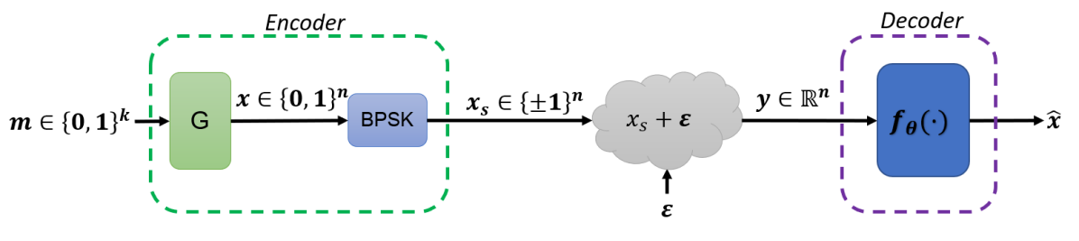
The input message is encoded by to a codeword satisfying and transmitted via a symmetric (potentially binary) channel,e.g., an additive white Gaussian noise (AWGN) channel. Let denote the channel output represented as , where denotes the modulation of , e.g. Binary Phase Shift Keying (BPSK), and is random noise independent of the transmitted . The main goal of the decoder is to provide an approximation of the codeword .
An important notion in ECC is the syndrome, which is obtained by multiplying the binary mapping of with the parity check matrix over such that
| (1) |
where denotes the XOR operator, and and denote the hard-decision vectors of and , respectively.
Quantum Error Correction Code The fundamental transition to the quantum realm is defined by the shift from the classical bit to the quantum bit (qubit), whose quantum state is defined by
| (2) |
A coherent quantum error process can be decomposed into a sum of operators from the Pauli set , where the Pauli basis is defined by the identity mapping , the quantum bit-flip and the phase-flip , such that
| (3) | ||||
and where the single-qubit error is defined as
| (4) |
with being the expansion coefficients of the noise process.
According to the no-cloning theorem, a quantum state cannot be copied redundantly (i.e. ), where denotes the -fold tensor product. However, quantum information redundancy is possible through a logical state encoding of a given state via quantum entanglement and a unitary operator such that . An example of such a unitary operator is the GHZ state (Greenberger, Horne, and Zeilinger 1989), which is generated with CNOT gates. In , the logical state is defined within a subspace of the expanded Hilbert space, which determines both the codespace and its orthogonal error space defined such that .
The orthogonality of and makes it possible to determine the subspace occupied by the logical qubit through projective measurement, without compromising the encoded quantum information. In the context of quantum coding, the set of non-destructive measurements of this type are called stabilizer measurements and are performed via additional qubits (ancilla bits). The result of all of the stabilizer measurements on a given state is called the syndrome, such that for a given stabilizer generator we have , and , given an anti-commuting (i.e. eigenvalue) and thus detectable error . If the syndrome measurement is faulty, it might be necessary to repeat it to improve confidence in the outcome (Dennis et al. 2002, Section IV.B).
An important class of Pauli operators is the class of logical operators. These operators are not elements of the stabilizer group but commute with every stabilizer. While stabilizers operators act trivially in the code space, i.e. , logical operators act non-trivially in it, i.e. . Such operators commute with the stabilizers but can also represent undetectable errors (Brun 2020). Thus, similarly to the classical information bits, QECC benchmarks generally adopt logical error metrics, which measure the discrepancy between the predicted projected noise and the real one , where is the discrete logical operators’ matrix.
QECC from the ECC perspective Another way to represent stabilizer codes is to split the stabilizer operators into two independent parity check matrices, defining the block parity check matrix such that , separating phase-flip checks and bit-flip checks . The syndrome is then computed as , being the check-matrix defined according to the code stabilizers in , and the binary noise. The main goal of the quantum decoder is to provide a noise approximation given only the syndrome.
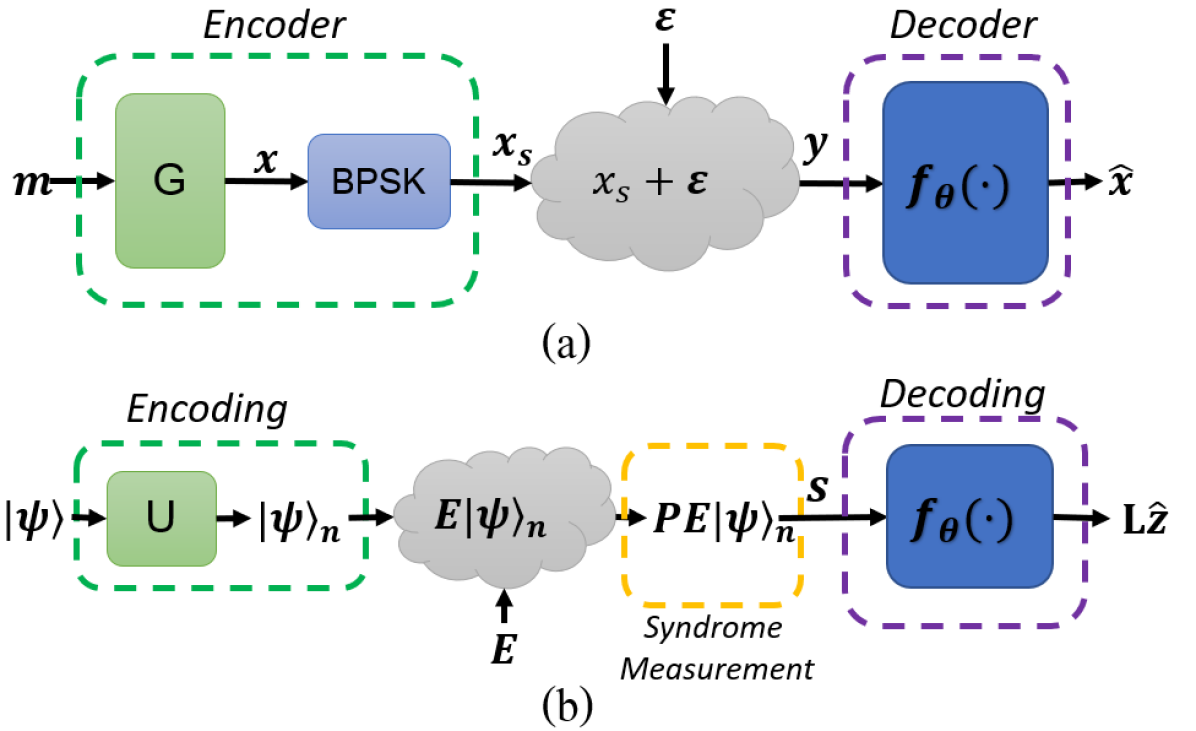
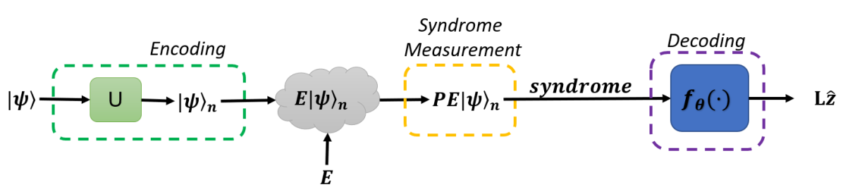
Therefore, the quantum setting can be reduced to its classical counterpart as follows. The logical qubits are similar to the classical information bits, and the physical qubits are similar to the classical codeword. The syndrome of the quantum state can be computed or simulated similarly to the classical way, by defining the binary parity check matrix built upon the code quantum stabilizers. The main differences from classical ECC are: (i) no access to the current state is possible, while arbitrary measurement of is standard in the classical world; (ii) we are interested in the logical qubits, predicting the code up to the logical operators mapping ; and finally, (iii) repetitive sampling of the syndrome due to the syndrome measurement error. These differences are at the core of our contributions. An illustration of the classical and quantum coding and decoding framework is given in Figure 1. The goal of our method is to learn a decoder parameterized by weights such that .
Error Correction Code Transformer The SOTA ECCT (Choukroun and Wolf 2022) has been recently proposed for classical error decoding. It consists of a transformer architecture (Vaswani et al. 2017) with several modifications.
Following (Bennatan, Choukroun, and Kisilev 2018), the model’s input is defined by the concatenation of the codeword-independent magnitude and syndrome, such that where denotes vector concatenation. Each element is then embedded into a high-dimensional space for more expressivity, such that the initial positional embedding is given by , where is the learnable embedding matrix and is the Hadamard product.
The interaction between the bits is performed naturally via the self-attention modules coupled with a binary mask derived from the parity-check matrix
| (5) |
where is a binary masking function designed according to the parity-check matrix , and are the classical self-attention projection matrices. Masking enables the incorporation of sparse and efficient information about the code while avoiding the loop vulnerability of belief propagation-based decoders (Pearl 1988). Finally, the transformed embedding is projected onto a one-dimensional vector for noise prediction. The computational complexity is , where denotes the number of layers, and is the code length. Here, denotes the number of elements in the mask, generally very small for sparse codes, including Toric and Surface codes.
Method
We present in this Section the elements of the proposed decoding framework, the complete architecture, and the training procedure. From now on, the binary block parity check matrix is denoted by , the binary noise by , the syndrome by , and the logical operators’ binary matrix by .
Overcoming Measurement Collapse by Prediction
While syndrome decoding is a well-known procedure in ECC, most popular decoders, and especially neural decoders, assume the availability of arbitrary measurements of the channel’s output. In the QECC setting, only the syndrome is available, since classical measurements are not allowed due to the wave function collapse phenomenon.
We thus propose to extend ECCT, by replacing the magnitude of the channel output with an initial estimate of the noise to be further refined by the code-aware network. In other words, we replace the channel’s output magnitude measurement by .
Denoting the ECCT decoder by we have
| (6) |
where is the initial noise estimator, given by a shallow neural network parameterized by . This way, the ECCT can process the estimated input and perform decoding by analyzing the input-syndrome interactions via the masking. As a non-linear transformation of the syndrome, is also independent of the quantum state/codeword and thus robust to overfitting. The estimator is trained via the following objective
| (7) |
where BCE is the binary cross entropy loss. This shift from magnitude to initial error estimation is crucial for overcoming quantum measurement collapse and, as explored in the analysis section, leads to markedly better performance.
Logical Decoding
Contrary to classical ECC, quantum error correction aims to restore the noise up to a logical generator of the code, such that several solutions can be valid error correction. Accordingly, the commonly used metric is the logical error rate (LER), which provides valuable information on the practical decoding performance (Lidar and Brun 2013). Given the code’s logical operator in its matrix form , we wish to minimize the following LER objective
| (8) |
where the multiplications are performed over (i.e. binary modulo 2) and are thus highly non-differentiable.
We propose to optimize the objective using a differentiable equivalence mapping of the XOR (i.e., sum over ) operation as follows. Defining the bipolar mapping over as , we obtain the following property . Thus, with the -th row of and a binary vector, we have
| (9) |
Thus, as a composition of differentiable functions is differentiable and we can redefine our objective as folllows
| (10) |
where denotes the binarization of the soft prediction of the trained model. While many existing works make use of the straight-through estimator (STE) (Bengio, Léonard, and Courville 2013) for the binary quantization of the activations, we opt for its differentiable approximation with the sigmoid function (i.e., ). As shown in our ablation analysis, the performance of the STE is slightly inferior to the sigmoid approach.
In addition to directly minimizing the LER metric, we are interested in noise prediction solutions that are close to the real system noise. We, therefore, suggest regularizing the objective with the classical and popular Bit Error Rate (BER) objective defined as . Combining the loss terms, the overall objective is given by
| (11) |
where denote the weights of each objective.
Noisy Syndrome Measurements
In the presence of measurement errors, each syndrome measurement is repeated times. This gives the decoder input an additional time dimension. Formally, given binary system noises and binary measurement noises , we have the syndrome at a given time defined as
| (12) |
To remain invariant to the number of measurements, we first analyze each measurement separately and then perform global decoding by applying a symmetric pooling function, e.g. an average, in the middle of the neural decoder.
Given a NN decoder with layers and the hidden activation tensor at layer , the new pooled embedding is given by summation along the first dimension . The loss is thus defined as the distance between the pooled embedding and the noise, i.e.,
| (13) |
with the cumulative binary system noise.
Since we extend the ECCT architecture to its quantum counterpart (QECCT), the hidden activation tensor is now of shape with the number of self-attention heads, and pooling is performed at the Transformer block. An advantage of this approach is its low computational cost since the analysis and comparison are performed in parallel at the embedding level.
Architecture and Training
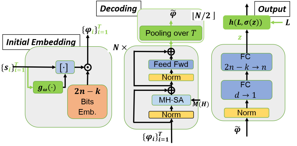
The initial encoding is defined as a dimensional one-hot encoding of the input elements where is the number of physical qubits and the length of the syndrome. The network is defined as a shallow network with two fully connected layers of hidden dimensions equal to and with a GELU non-linearity. The decoder is defined as a concatenation of decoding layers composed of self-attention and feed-forward layers interleaved with normalization layers. In case of faulty syndrome measurements, the th layer performs average pooling over the time dimension.
The output is obtained via two fully connected layers. The first layer reduces the element-wise embedding to a one-dimensional vector and the second to an dimensional vector representing the soft decoded noise, trained over the objective given Eq. 11. An illustration of the proposed QECCT is given in Figure 2.
The complexity of the network is linear with the code length and quadratic with the embedding dimension and is defined by for sparse (e.g. topological) codes. The acceleration of the proposed method (e.g. pruning, quantization, distillation, low-rank approximation) (Wang et al. 2020; Lin et al. 2021) is out of the scope of this paper and left for future work. For example, low-rank approximation would make the complexity also linear in (Wang et al. 2020). Also, no optimization of the sparse self-attention mechanism was employed in our implementation.
The Adam optimizer (Kingma and Ba 2014) is used with 512 samples per minibatch, for 200 to 800 epochs depending on the code length, with 5000 minibatches per epoch. The training is performed by randomly sampling noise in the physical error rate testing range. The default weight parameters are . Other configurations and longer training can be beneficial but were not tested due to a lack of computational resources. The default architecture is .
We initialized the learning rate to coupled with a cosine decay scheduler down to at the end of training. No warmup (Xiong et al. 2020) was employed.
Training and experiments were performed on a 12GB Titan V GPU. The training time ranges from 153 to 692 seconds per epoch for the 32 to 400 code lengths, respectively with the default architecture. Test time is in the range of 0.1 to 0.6 milliseconds per sample. The number of testing samples is set to , enough to obtain a small standard deviation () between experiments.
Application to Topological Codes
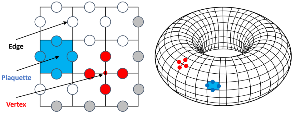
While our framework is universal in terms of the code, we focus on the popular Surface codes and, more specifically, on Toric codes (Kitaev 1997a, b, 2003), which are their variant with periodic boundary conditions. These codes are among the most attractive candidates for quantum computing experimental realization, as they can be implemented on a two-dimensional grid of qubits with local check operators (Bravyi et al. 2018). The physical qubits are placed on the edges of a two-dimensional lattice of length , such that the stabilizers are defined with respect to the code lattice architecture that defines the codespace, where .
The stabilizers are defined in two groups: vertex operators are defined on each vertex as the product of operators on the adjacent qubits and plaquette operators are defined on each face as the product of operators on the bordering qubits. Therefore, there exist a total of stabilizers, for each stabilizer group. Assuming that a qubit is associated with every edge of the lattice, for a given vertex we have the vertex operator defined as , and for a given plaquette , the plaquette operator defined as . An illustration is given in Appendix G.
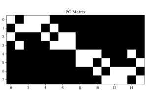
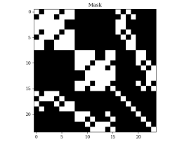
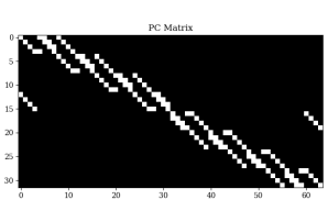
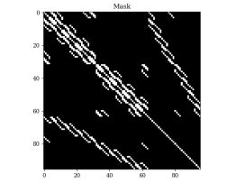
The mask is defined such that the self-attention mechanism only takes into consideration bits related to each other in terms of the stabilizers (i.e., the parity-check matrix). The parity-check matrices and their corresponding masks for several Toric codes are provided in Figure 3, where one can observe the high locality induced by the code architecture (the mask only reflects stabilizers-related elements).
 |
 |
 |
 |
| (a) | (b) | (c) | (d) |
Experiments
We evaluate our method on various Toric code lengths, considering the two common noise models: independent and depolarization. In independent (uncorrelated) noise, and errors occur independently and with equal probabilities; therefore, decoding can be performed on the or stabilizers separately. Depolarization noise assigns equal probability to all three Pauli operators , where is the Pauli operator defined as .
In the experiments where measurement errors are incorporated, each syndrome measurement is repeated times and the probability of the measurement error is the same as the probability of the syndrome error, i.e., the distributions of and in Eq. 12 are the same as in (Dennis et al. 2002; Higgott 2022; Wang, Harrington, and Preskill 2003).
The implementation of the Toric codes is taken from (Krastanov and Jiang 2017). As a baseline, we consider the Minimum-Weight Perfect Matching (MWPM) algorithm with the complexity of , also known as the Edmond or Blossom algorithm, which is the most popular decoder for topological codes. Its implementation is taken from (Higgott and Gidney 2022; Higgott 2022) and is close to quadratic average complexity. In the experiments, we employ code lengths similar to those for which the existing end-to-end neural decoders were tested, i.e., (Varsamopoulos, Criger, and Bertels 2017; Torlai and Melko 2017; Krastanov and Jiang 2017; Chamberland and Ronagh 2018; Andreasson et al. 2019; Wagner, Kampermann, and Bruß 2020). It is worth noting that none of these previous methods outperform MWPM. The physical error ranges are taken around the thresholds of the different settings, as reported in (Dennis et al. 2002; Wang, Harrington, and Preskill 2003; Krastanov and Jiang 2017). On the tested codes and settings, the Union-find decoder (Park and Meinerz 2022) was not better than the MWPM algorithm.
As metrics, we present both the bit error rates (BER) and the logical error rate (LER), see the Logical Decoding section. The LER metric here is a word-level error metric, meaning there is an error if at least one qubit is different from the ground truth.
Results
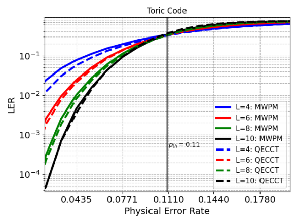
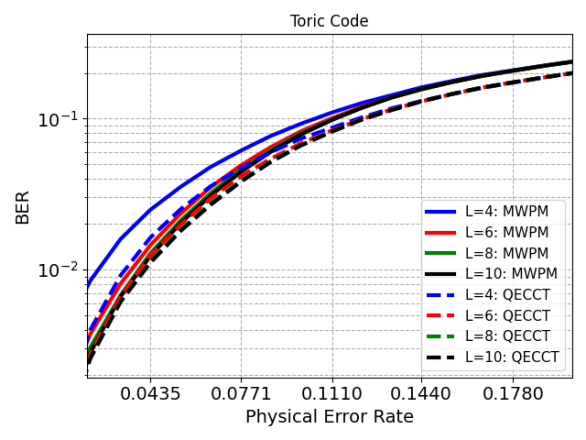
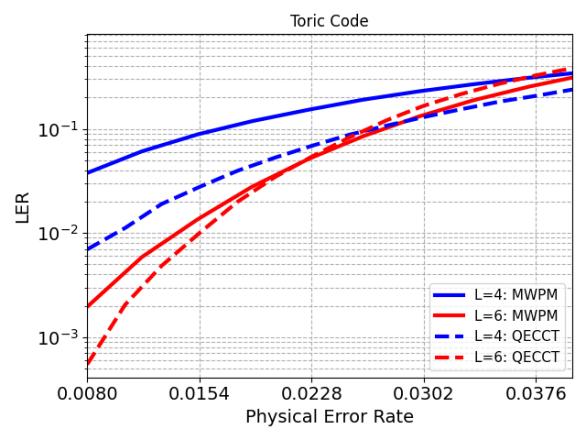
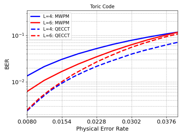
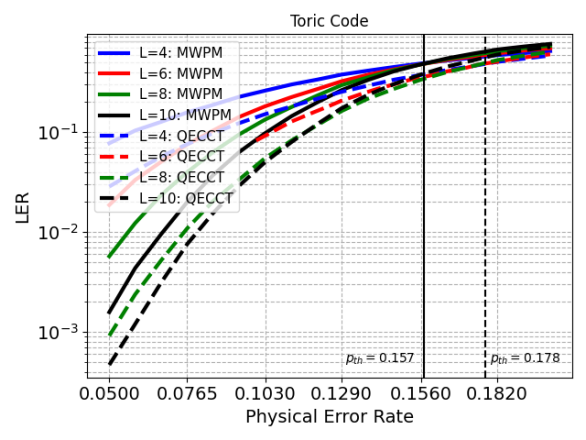
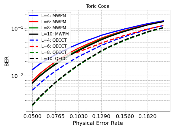
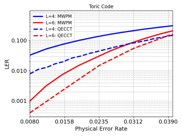
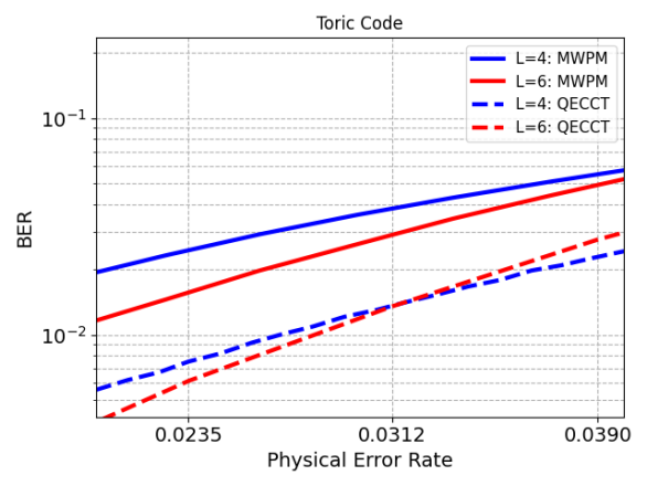
Figure 4 depicts the performance of the proposed method and the MWPM algorithm for different Toric code lengths under the independent noise model and without noisy measurements. Figure 5 presents a similar comparison with noisy measurements with and uniformly distributed syndrome error. Figure 6 and 7 compare our method with MWPM for the depolarized noise model, with and without noisy measurements, respectively. We also provide the obtained threshold values.
As can be seen, the proposed QECCT outperforms the SOTA MWPM algorithm by a large margin: (i) QECCT outperforms the MWPM algorithm on independent noise, where MWPM is known to almost reach ML’s threshold (Dennis et al. 2002), and (ii) QECCT outperforms the SOTA MWPM on the challenging depolarization noise setting by a large margin, where the obtained threshold is 0.178 compared to 0.157 for MWPM and 0.189 for ML (Bombin et al. 2012). The very large gaps in BER imply that the proposed method is able to better detect exact corruptions. The threshold is slightly lower for with depolarization noise while the BER is much lower, denoting a potential need for tuning the regularization parameter for larger code. In Appendix B we present performance statistics for the vanilla MLP decoder with similar capacity, highlighting both the contribution of our architecture and the importance of the proposed regularization term.
 |
 |
 |
 |
 |
 |
 |
 |
 |
 |
 |
 |
| (a) | (b) |
Further Validation and an Ablation Study
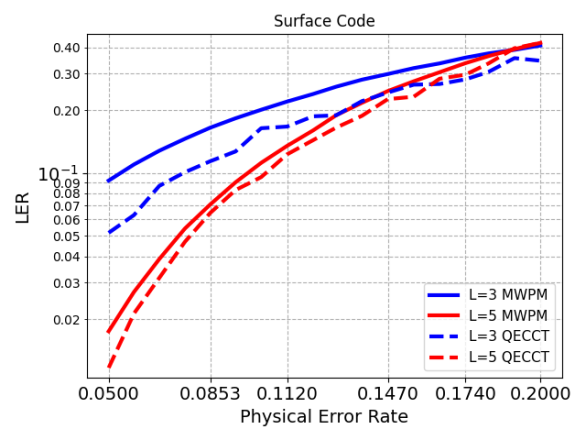
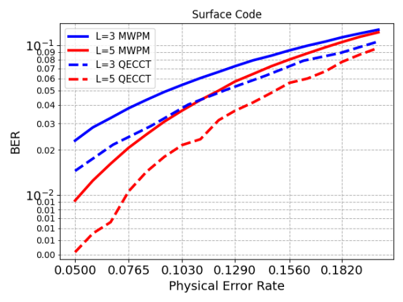
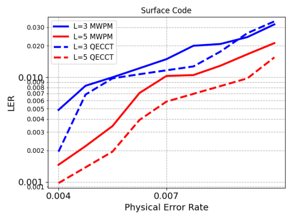
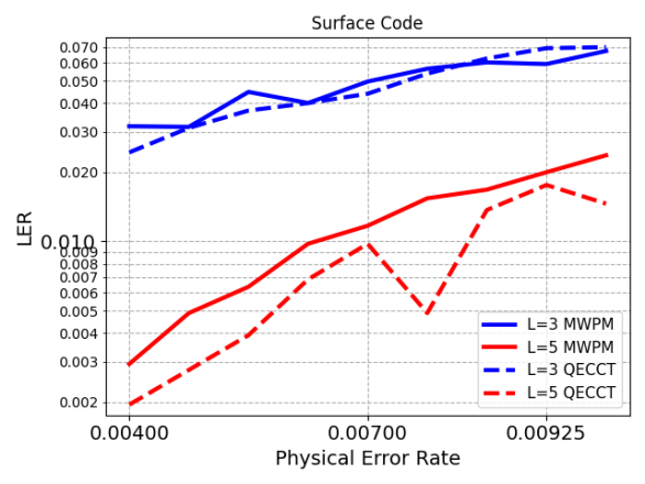
We extend our experiments beyond what is commonly done in the relevant ML work. To check that the method is applicable not just for Toric codes, Figure 8 shows the performance for different Surface code lengths of the proposed method and the MWPM algorithm under the depolarization noise model. The same parameters as were used for Toric codes are used here. As can be seen, the method is able to similarly outperform MWPM for other codes as well. The large gap in BER in favor of the QECCT probably means that the gap in LER can be made larger with other hyperparameters of the objective.
To explore the generality with respect to noise models, Figure 9 shows the performance under the circuit noise model of the proposed method and the MWPM algorithm for different Surface code lengths. The channel is simulated using the STIM (Gidney 2021) simulator of quantum stabilizer circuits where the same depolarization error probability is applied after every single and two-qubit Clifford operation, before every stabilizer measurement, and before the syndrome measurement. Evidently, the proposed method is able to consistently outperform MWPM for this type of channel noise as well.
The impact of the noise estimator is studied in Appendix C, where it is shown that the initial noise estimator is critical for performance. The impact of the various objectives in Eq. 11 is provided in Appendix D. It is demonstrated via the gradient norm that training solely with the objective converges rapidly to a bad local minimum. Training with only produces far worse results than combining it with the objective. For high SNR, a model trained with objective yields a 27 times higher LER than the model trained with combined objectives. Moreover, optimizing with the noise estimator objective results, for high SNR, in a 46% improvement over not employing regularization. The impact of Pooling is explored in Appendix E, where various scenarios are compared. Empirical evidence is provided to support pooling in the middle layer, as suggested. Finally, the impact of the mask and the architecture is explored in Appendix F. Specifically, masking, the model’s capacity, and the STE as function from Eq 10 are being evaluated. We can observe that while less important than with classical codes (Choukroun and Wolf 2022), the mask still substantially impacts performance. Also, we note increasing the capacity of the network enables better representation and decoding.
Limitations While the proposed method has a smaller complexity than classical SOTA, its implementation in a straightforward way makes it difficult to train for larger codes or more repetitions, e.g. unstructured sparse self-attention is not easy to implement on general-purpose DL accelerators. Larger architectures and longer training times would enable larger code correction and are expected to also improve accuracy, deepening the gap from other methods. As a point of reference, GPT-3 (Brown et al. 2020) successfully operates on 2K inputs with a similar Transformer model but with .
Conclusion
We present a novel Transformer-based framework for decoding quantum codes, offering multiple technical contributions enabling the effective representation and training under the QECC constraints. First, the framework helps overcome the measurement collapse phenomenon by predicting the noise and then refining it. Second, we present a novel paradigm for differentiable training of highly non-differentiable functions, with far-reaching implications for ML-based error correction. Finally, we propose a time-efficient and size-invariant pooling for faulty measurement scenarios. Since the lack of effective and efficient error correction is a well-known limiting factor for the development of quantum computers, our contribution can play a role in using machine learning tools for overcoming the current technological limitations of many-qubit systems.
References
- Aharonov and Ben-Or (1997) Aharonov, D.; and Ben-Or, M. 1997. Fault-tolerant quantum computation with constant error. In Proceedings of the twenty-ninth annual ACM symposium on Theory of computing, 176–188.
- Andreasson et al. (2019) Andreasson, P.; Johansson, J.; Liljestrand, S.; and Granath, M. 2019. Quantum error correction for the toric code using deep reinforcement learning. Quantum, 3: 183.
- Ballance et al. (2016) Ballance, C.; Harty, T.; Linke, N.; Sepiol, M.; and Lucas, D. 2016. High-fidelity quantum logic gates using trapped-ion hyperfine qubits. Physical review letters, 117(6): 060504.
- Bengio, Léonard, and Courville (2013) Bengio, Y.; Léonard, N.; and Courville, A. 2013. Estimating or propagating gradients through stochastic neurons for conditional computation. arXiv preprint arXiv:1308.3432.
- Bennatan, Choukroun, and Kisilev (2018) Bennatan, A.; Choukroun, Y.; and Kisilev, P. 2018. Deep learning for decoding of linear codes-a syndrome-based approach. In 2018 IEEE International Symposium on Information Theory (ISIT), 1595–1599. IEEE.
- Bombin et al. (2012) Bombin, H.; Andrist, R. S.; Ohzeki, M.; Katzgraber, H. G.; and Martin-Delgado, M. A. 2012. Strong resilience of topological codes to depolarization. Physical Review X, 2(2): 021004.
- Bose and Dowling (1969) Bose, R. C.; and Dowling, T. 1969. Combinatorial mathematics and its applications: proceedings of the conference held at the University of North Carolina at Chapel Hill, April 10-14, 1967. 4. University of North Carolina Press.
- Bravyi et al. (2018) Bravyi, S.; Englbrecht, M.; König, R.; and Peard, N. 2018. Correcting coherent errors with surface codes. npj Quantum Information, 4(1): 1–6.
- Bravyi and Kitaev (1998) Bravyi, S. B.; and Kitaev, A. Y. 1998. Quantum codes on a lattice with boundary. arXiv preprint quant-ph/9811052.
- Brown et al. (2020) Brown, T.; Mann, B.; Ryder, N.; Subbiah, M.; Kaplan, J. D.; Dhariwal, P.; Neelakantan, A.; Shyam, P.; Sastry, G.; Askell, A.; et al. 2020. Language models are few-shot learners. Advances in neural information processing systems, 33: 1877–1901.
- Brun (2020) Brun, T. A. 2020. Quantum Error Correction.
- Buchberger et al. (2020) Buchberger, A.; Häger, C.; Pfister, H. D.; Schmalen, L.; et al. 2020. Learned Decimation for Neural Belief Propagation Decoders. arXiv preprint arXiv:2011.02161.
- Calderbank and Shor (1996) Calderbank, A. R.; and Shor, P. W. 1996. Good quantum error-correcting codes exist. Physical Review A, 54(2): 1098.
- Cammerer et al. (2017) Cammerer, S.; Gruber, T.; Hoydis, J.; and ten Brink, S. 2017. Scaling deep learning-based decoding of polar codes via partitioning. In GLOBECOM 2017-2017 IEEE Global Communications Conference, 1–6. IEEE.
- Chamberland and Ronagh (2018) Chamberland, C.; and Ronagh, P. 2018. Deep neural decoders for near term fault-tolerant experiments. Quantum Science and Technology, 3(4): 044002.
- Choukroun and Wolf (2022) Choukroun, Y.; and Wolf, L. 2022. Error Correction Code Transformer. Advances in Neural Information Processing Systems (NeurIPS).
- Choukroun and Wolf (2023) Choukroun, Y.; and Wolf, L. 2023. Denoising Diffusion Error Correction Codes. International Conference on Learning Representations (ICLR).
- Cory et al. (1998) Cory, D. G.; Price, M.; Maas, W.; Knill, E.; Laflamme, R.; Zurek, W. H.; Havel, T. F.; and Somaroo, S. S. 1998. Experimental quantum error correction. Physical Review Letters, 81(10): 2152.
- Delfosse and Nickerson (2021) Delfosse, N.; and Nickerson, N. H. 2021. Almost-linear time decoding algorithm for topological codes. Quantum, 5: 595.
- Dennis et al. (2002) Dennis, E.; Kitaev, A.; Landahl, A.; and Preskill, J. 2002. Topological quantum memory. Journal of Mathematical Physics, 43(9): 4452–4505.
- Duclos-Cianci and Poulin (2010) Duclos-Cianci, G.; and Poulin, D. 2010. Fast decoders for topological quantum codes. Physical review letters, 104(5): 050504.
- Duclos-Cianci and Poulin (2013) Duclos-Cianci, G.; and Poulin, D. 2013. Fault-tolerant renormalization group decoder for abelian topological codes. arXiv preprint arXiv:1304.6100.
- Edmonds (1965) Edmonds, J. 1965. Paths, trees, and flowers. Canadian Journal of mathematics, 17: 449–467.
- Fowler (2013) Fowler, A. G. 2013. Minimum weight perfect matching of fault-tolerant topological quantum error correction in average parallel time. arXiv preprint arXiv:1307.1740.
- Fowler, Whiteside, and Hollenberg (2012) Fowler, A. G.; Whiteside, A. C.; and Hollenberg, L. C. 2012. Towards practical classical processing for the surface code. Physical review letters, 108(18): 180501.
- Foxen et al. (2020) Foxen, B.; Neill, C.; Dunsworth, A.; Roushan, P.; Chiaro, B.; Megrant, A.; Kelly, J.; Chen, Z.; Satzinger, K.; Barends, R.; et al. 2020. Demonstrating a continuous set of two-qubit gates for near-term quantum algorithms. Physical Review Letters, 125(12): 120504.
- Gidney (2021) Gidney, C. 2021. Stim: a fast stabilizer circuit simulator. Quantum, 5: 497.
- Gottesman (1997) Gottesman, D. 1997. Stabilizer codes and quantum error correction. California Institute of Technology.
- Greenberger, Horne, and Zeilinger (1989) Greenberger, D. M.; Horne, M. A.; and Zeilinger, A. 1989. Going beyond Bell’s theorem. In Bell’s theorem, quantum theory and conceptions of the universe, 69–72. Springer.
- Gruber et al. (2017) Gruber, T.; Cammerer, S.; Hoydis, J.; and ten Brink, S. 2017. On deep learning-based channel decoding. In 2017 51st Annual Conference on Information Sciences and Systems (CISS), 1–6. IEEE.
- Higgott (2022) Higgott, O. 2022. PyMatching: A Python package for decoding quantum codes with minimum-weight perfect matching. ACM Transactions on Quantum Computing, 3(3): 1–16.
- Higgott and Gidney (2022) Higgott, O.; and Gidney, C. 2022. PyMatching v2. https://github.com/oscarhiggott/PyMatching.
- Huang, Newman, and Brown (2020) Huang, S.; Newman, M.; and Brown, K. R. 2020. Fault-tolerant weighted union-find decoding on the toric code. Physical Review A, 102(1): 012419.
- Huang et al. (2019) Huang, W.; Yang, C.; Chan, K.; Tanttu, T.; Hensen, B.; Leon, R.; Fogarty, M.; Hwang, J.; Hudson, F.; Itoh, K. M.; et al. 2019. Fidelity benchmarks for two-qubit gates in silicon. Nature, 569(7757): 532–536.
- Hutter, Wootton, and Loss (2014) Hutter, A.; Wootton, J. R.; and Loss, D. 2014. Efficient Markov chain Monte Carlo algorithm for the surface code. Physical Review A, 89(2): 022326.
- Kim et al. (2018) Kim, H.; Jiang, Y.; Rana, R.; Kannan, S.; Oh, S.; and Viswanath, P. 2018. Communication algorithms via deep learning. In Sixth International Conference on Learning Representations (ICLR).
- Kingma and Ba (2014) Kingma, D. P.; and Ba, J. 2014. Adam: A method for stochastic optimization. arXiv preprint arXiv:1412.6980.
- Kitaev (1997a) Kitaev, A. Y. 1997a. Quantum computations: algorithms and error correction. Russian Mathematical Surveys, 52(6): 1191.
- Kitaev (1997b) Kitaev, A. Y. 1997b. Quantum computations: algorithms and error correction. Russian Mathematical Surveys, 52(6): 1191.
- Kitaev (1997c) Kitaev, A. Y. 1997c. Quantum error correction with imperfect gates. In Quantum communication, computing, and measurement, 181–188. Springer.
- Kitaev (2003) Kitaev, A. Y. 2003. Fault-tolerant quantum computation by anyons. Annals of Physics, 303(1): 2–30.
- Kolmogorov (2009) Kolmogorov, V. 2009. Blossom V: a new implementation of a minimum cost perfect matching algorithm. Mathematical Programming Computation, 1(1): 43–67.
- Krastanov and Jiang (2017) Krastanov, S.; and Jiang, L. 2017. Deep neural network probabilistic decoder for stabilizer codes. Scientific reports, 7(1): 1–7.
- Kuo and Lu (2020) Kuo, K.-Y.; and Lu, C.-C. 2020. On the hardnesses of several quantum decoding problems. Quantum Information Processing, 19(4): 1–17.
- Lidar and Brun (2013) Lidar, D. A.; and Brun, T. A. 2013. Quantum error correction. Cambridge university press.
- Lin et al. (2021) Lin, T.; Wang, Y.; Liu, X.; and Qiu, X. 2021. A survey of transformers. arXiv preprint arXiv:2106.04554.
- Lugosch and Gross (2017) Lugosch, L.; and Gross, W. J. 2017. Neural offset min-sum decoding. In 2017 IEEE International Symposium on Information Theory (ISIT), 1361–1365. IEEE.
- MacKay (2003) MacKay, D. J. 2003. Information theory, inference and learning algorithms. Cambridge university press.
- Meinerz, Park, and Trebst (2022) Meinerz, K.; Park, C.-Y.; and Trebst, S. 2022. Scalable neural decoder for topological surface codes. Physical Review Letters, 128(8): 080505.
- Micali and Vazirani (1980) Micali, S.; and Vazirani, V. V. 1980. An O (v— v— c— E—) algoithm for finding maximum matching in general graphs. In 21st Annual Symposium on Foundations of Computer Science (sfcs 1980), 17–27. IEEE.
- Nachmani, Be’ery, and Burshtein (2016) Nachmani, E.; Be’ery, Y.; and Burshtein, D. 2016. Learning to decode linear codes using deep learning. In 2016 54th Annual Allerton Conference on Communication, Control, and Computing (Allerton), 341–346. IEEE.
- Nachmani and Wolf (2019) Nachmani, E.; and Wolf, L. 2019. Hyper-graph-network decoders for block codes. In Advances in Neural Information Processing Systems, 2326–2336.
- Neumann, Wigner, and Hofstadter (1955) Neumann, J.; Wigner, E. P.; and Hofstadter, R. 1955. Mathematical foundations of quantum mechanics. Princeton university press.
- Nielsen and Chuang (2002) Nielsen, M. A.; and Chuang, I. 2002. Quantum computation and quantum information.
- Park and Meinerz (2022) Park, C.-Y.; and Meinerz, K. 2022. Open-source C++ implementation of the Union-Find decoder, https://github.com/chaeyeunpark/UnionFind. Physical Review Letters, 128(8): 080505.
- Pearl (1988) Pearl, J. 1988. Probabilistic reasoning in intelligent systems: networks of plausible inference. Morgan kaufmann.
- Preskill (1998) Preskill, J. 1998. Reliable quantum computers. Proceedings of the Royal Society of London. Series A: Mathematical, Physical and Engineering Sciences, 454(1969): 385–410.
- Raimond and Haroche (1996) Raimond, J.; and Haroche, S. 1996. Quantum computing: dream or nightmare. DARK MATTER IN COSMOLOGY QUANTUM MEASUREMENTS EXPERIMENTAL GRA VITA Tl ON, 341.
- Schindler et al. (2011) Schindler, P.; Barreiro, J. T.; Monz, T.; Nebendahl, V.; Nigg, D.; Chwalla, M.; Hennrich, M.; and Blatt, R. 2011. Experimental repetitive quantum error correction. Science, 332(6033): 1059–1061.
- Shannon (1948) Shannon, C. E. 1948. A mathematical theory of communication. The Bell system technical journal, 27(3): 379–423.
- Shor (1995) Shor, P. W. 1995. Scheme for reducing decoherence in quantum computer memory. Physical review A, 52(4): R2493.
- Sweke et al. (2020) Sweke, R.; Kesselring, M. S.; van Nieuwenburg, E. P.; and Eisert, J. 2020. Reinforcement learning decoders for fault-tolerant quantum computation. Machine Learning: Science and Technology, 2(2): 025005.
- Torlai and Melko (2017) Torlai, G.; and Melko, R. G. 2017. Neural decoder for topological codes. Physical review letters, 119(3): 030501.
- Varona and Martin-Delgado (2020) Varona, S.; and Martin-Delgado, M. A. 2020. Determination of the semion code threshold using neural decoders. Physical Review A, 102(3): 032411.
- Varsamopoulos, Criger, and Bertels (2017) Varsamopoulos, S.; Criger, B.; and Bertels, K. 2017. Decoding small surface codes with feedforward neural networks. Quantum Science and Technology, 3(1): 015004.
- Vaswani et al. (2017) Vaswani, A.; Shazeer, N.; Parmar, N.; Uszkoreit, J.; Jones, L.; Gomez, A. N.; Kaiser, Ł.; and Polosukhin, I. 2017. Attention is all you need. In Advances in neural information processing systems, 5998–6008.
- Wagner, Kampermann, and Bruß (2020) Wagner, T.; Kampermann, H.; and Bruß, D. 2020. Symmetries for a high-level neural decoder on the toric code. Physical Review A, 102(4): 042411.
- Wang, Harrington, and Preskill (2003) Wang, C.; Harrington, J.; and Preskill, J. 2003. Confinement-Higgs transition in a disordered gauge theory and the accuracy threshold for quantum memory. Annals of Physics, 303(1): 31–58.
- Wang et al. (2020) Wang, S.; Li, B. Z.; Khabsa, M.; Fang, H.; and Ma, H. 2020. Linformer: Self-attention with linear complexity. arXiv preprint arXiv:2006.04768.
- Wootters and Zurek (1982) Wootters, W. K.; and Zurek, W. H. 1982. A single quantum cannot be cloned. Nature, 299(5886): 802–803.
- Wootton and Loss (2012) Wootton, J. R.; and Loss, D. 2012. High threshold error correction for the surface code. Physical review letters, 109(16): 160503.
- Xiong et al. (2020) Xiong, R.; et al. 2020. On layer normalization in the transformer architecture. arXiv:2002.04745.
Appendix A A. Classical vs. Quantum Error Correction
We present in Fig. 10 a more detailed version of Fig.1 in the main paper, illustrating the differences between classical and quantum error correction. These differences are detailed in the main text.
 |
| (a) |
 |
| (b) |
Appendix B B. MLP Decoder
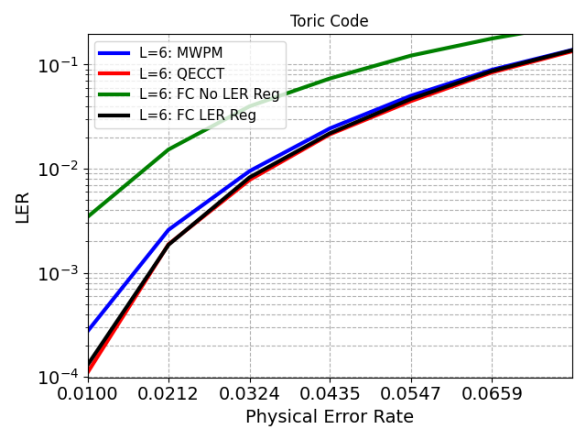
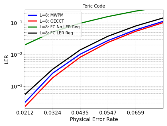
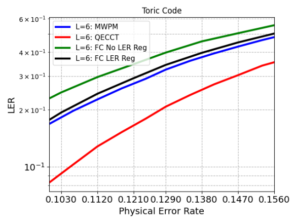
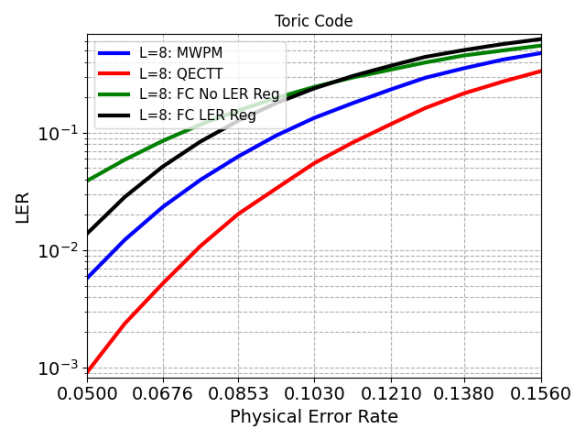
We present below the results obtained with Fully-Connected (FC) models on the L=6 and L=8 codes under the same training and capacity budgets as the QECCT. We present the best FC results, obtained using 10 layers and d=256-dimensional embedding on high SNRs.
These results are obtained after experimenting with different architecture parameters. The use of CNN and RNN is not well defined in our one-dimensional input setting and thus not experimented with.
We can observe in Figures 11 and 12 that our model outperforms the deep FCNN and is especially suitable for larger codes and depolarization noise where the correlation between the X and Z errors can be considered via the pairwise self-attention mechanism. Also, we can observe the advantage of the LER regularization which can bring orders of magnitude in the improvement of the accuracy and make the MLP model comparable to MWPM.
 |
 |
 |
 |
Appendix C C. Impact of the noise estimator
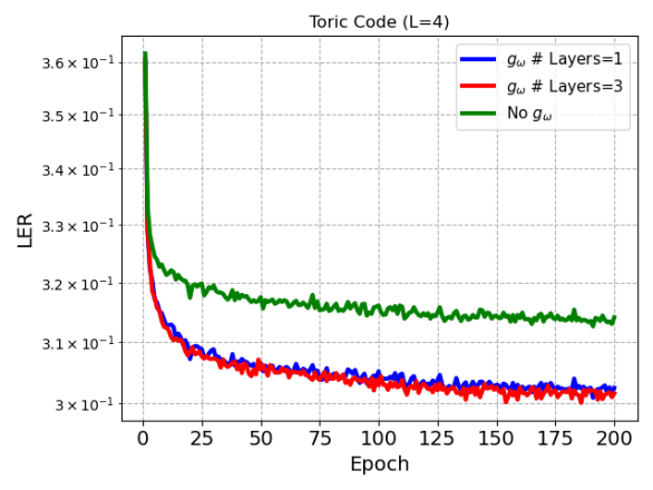
Figure 13(a) explores the impact of on performance. Since in order to use the QECCT the initial scaling estimate needs to be defined, we compare our approach to constant scaling with ones, meaning . We further explore two architectures for : one with a single hidden layer and one with three hidden layers. Evidently, the initial noise estimator is critical for performance. However, the network architecture is less impactful. Given more resources, one can check the impact of additional architectures.
 |
 |
|
| (a) | (b) |
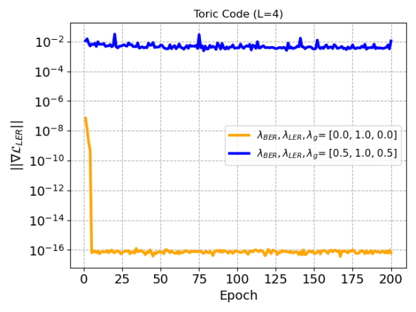
Appendix D D. Impact of the various objectives
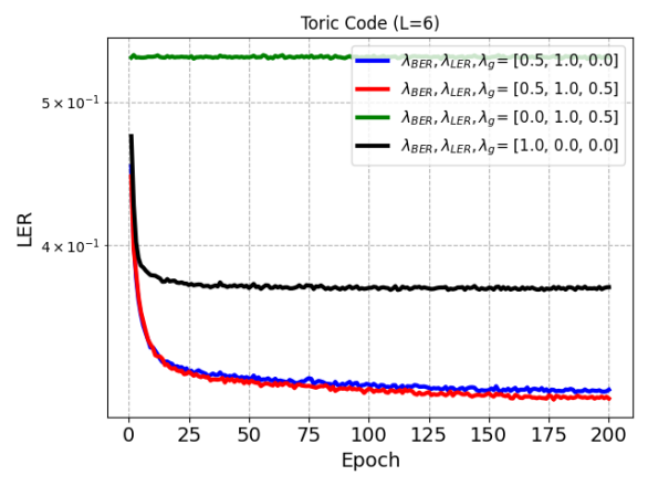
Figure 14(a) depicts the impact of the different loss terms of the training objective. First, we can observe that training solely with the objective converges rapidly to a bad local minimum. This is illustrated in Figure 14(b) where we display the gradient norm average over the network layers.
We hypothesize that this issue may be due to the fact that the dimension of the LER objective is rather small and the gradients can collapse in the product of the code elements in Eq 9, since . Also, the product of the elements allows the creation of a saddle point objective.
Evidently, training with only produces far worse results than combining it with the objective. For high SNR, a model trained with objective yields a 27 times higher LER than the model trained with combined objectives. Moreover, optimizing with the noise estimator objective results, for high SNR, in a 46% improvement over not employing regularization.
 |
 |
|
| (a) | (b) |
Appendix E E. Impact of Pooling
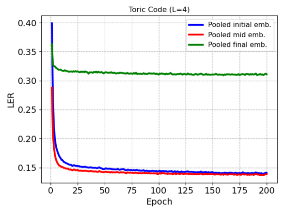
Figure 13(b) depicts the impact of different pooling (averaging) scenarios. Pooling is performed either after the initial embedding, in the middle of the network, or over the final embedding. Evidently, performing pooling in the middle layer allows better decoding. Pooling the final embedding (similarly to voting) is not effective.
 |
 |
|
| (a) | (b) |
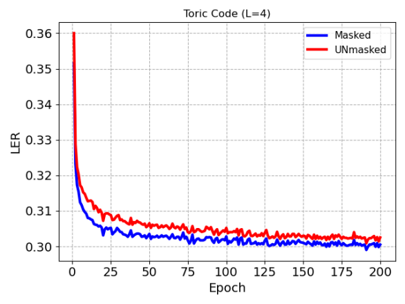
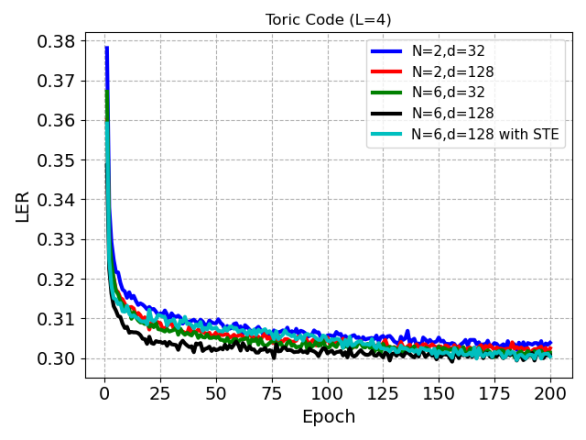
Appendix F F. Impact of the Mask and the Architecture
Finally, we present the impact of masking in Figure 15(a) and the impact of the model’s capacity and the performance of the STE as function in Figure 15(b). We can observe that while less important than with classical codes (Choukroun and Wolf 2022), the mask still substantially impacts performance. Also, we note that increasing the capacity of the network enables better representation and decoding.
Appendix G G. Toric Codes
We provide an illustration of the Toric code in Figure 16.