High-frequency complex impedance analysis of the two-dimensional semiconducting MXene-$\bf{Ti_{2}CO_{2}}$

Abstract

The two-dimensional compound group of MXenes, which exhibit unique optical, electrical, chemical, and mechanical properties, are an exceptional class of transition metal carbides and nitrides. In addition to traditional applications in Li-S, Li-ion batteries, conductive electrodes, hydrogen storage, and fuel cells, the low lattice thermal conductivity coupled with high electron mobility in the semiconducting oxygen-functionalized MXene Ti₂CO₂ has led to the recent interests in high-performance thermoelectric and nanoelectronic devices. Apart from the above dc- transport applications, it is crucial to also understand ac- transport across them, given the growing interest in applications surrounding wireless communications and transparent conductors. In this work, we investigate using our recently developed $ab\leavevmode\nobreak\ initio$ transport model, the real and imaginary components of electron mobility and conductivity to conclusively depict carrier transport beyond the room temperature for frequency ranges upto the terahertz range. We also contrast the carrier mobility and conductivity with respect to the Drude’s model to depict its inaccuracies for a meaningful comparison with experiments. Our calculations show the effect of acoustic deformation potential scattering, piezoelectric scattering, and polar optical phonon scattering mechanisms. Without relying on experimental data, our model requires inputs calculated from first principles using density functional theory. Our results set the stage for providing ab-initio based ac- transport calculations given the current research on MXenes for high frequency applications.

I Introduction

Two-dimensional (2D) materials Mas-Balleste et al. (2011); Novoselov et al. (2004); Geim (2009); Geim and Novoselov (2010); Neto et al. (2009); Novoselov et al. (2005); Akinwande et al. (2017) have unique optical, electrical, chemical, and mechanical properties and have received much attention over the last two decades due to their utility in optoelectronics Cheng et al. (2019), flexible electronics Kim et al. (2015), nanogenerators Wang and Song (2006), nanoelectromechanical systems Lee et al. (2018), sensing Cai et al. (2018) and terahertz (THz) frequency devices Lin and Liu (2013). The 2D compound group of MXenes Barsoum (2000); Barsoum and Radovic (2011); Naguib et al. (2011, 2012a, 2014); Ghidiu et al. (2014) are an exceptional class of transition metal carbides and nitrides. In addition to traditional applications in Li-S Liang et al. (2015), Li-ion batteries (LIBs) Naguib et al. (2012b); Tian et al. (2019); Xie et al. (2014); Tang et al. (2012); Liang et al. (2015); Er et al. (2014), conductive electrodes, Halim et al. (2014), hydrogen storage Hu et al. (2013); Kumar et al. (2021); Lei et al. (2015); Li et al. (2018); Hu et al. (2014), optics Wang et al. (2020); Jiang et al. (2020); Fu et al. (2021); Xue et al. (2017), and fuel cells Xie et al. (2013), the narrow bandgap, improved thermodynamic stability, high Seebeck coefficient, high figure of merit, and the low lattice thermal conductivity coupled with high electron mobility in semiconducting and oxygen-functionalized 2D MXene Ti₂CO₂ has led to the recent interests in high-performance thermoelectric (TE) Gandi et al. (2016); Zha et al. (2016); Sarikurt et al. (2018) and nanoelectronic devices Kim and Alshareef (2019); Sarycheva et al. (2018). In the past few years, different modules Madsen and Singh (2006); Poncé et al. (2016); Faghaninia et al. (2015); Ganose et al. (2021) have been developed to predict dc transport properties of such materials with inputs calculated from the first-principles methods.
The importance of high-frequency analysis is growing due to the applicability of MXenes in developing thin and flexible antennas and for wearable and transparent electronic devices Sindhu et al. (2022); Lee et al. (2021); Ma et al. (2021); Zhang and Nicolosi (2019); Kim and Alshareef (2019). There are several aspects that function as restrictions, which makes it more challenging to fabricate such an antenna for wireless communication. The skin depth is one of them, which is frequency dependent. Apart from this, impedance matching is necessary, which further helps in determining the voltage standing wave ratio (VSWR). Typically, MXenes can match impedance at extremely small antenna thicknesses Sarycheva et al. (2018); Pozar (2009). Furthermore, the gain value depends on the thickness, and the gain values of all the MXene antennas decreases with decreasing thickness, which further emphasizes on accurate computation of frequency-dependent transport parameters. With the thickness and electrical conductivity, contributing majorly towards absorption, it is also possible to estimate the absorption loss for non-magnetic and conducting shielding materials Iqbal et al. (2020).
Given the myriad possibilities for high frequency operation of MXenes, and the paucity in the development of theoretical models, we advance an extended version of our previously developed module AMMCR Mandia et al. (2021) to obtain the highly accurate frequency-dependent electrical conductivity and other high frequency transport characteristics, which paves the way for the manufacturing of a variety of flexible, wearable, and nanoelectronic devices. Our model is based on the Rode’s iterative method Rode (1970a, 1973, 1975) evolved from the conventional semi-classical Boltzmann transport equation (BTE) Lundstrom (2002). We have included various scattering mechanisms explicitly. The variations in the characteristics across a wide range of temperatures, carrier concentrations, and frequencies are admirably captured by our model. Since our model does not rely on experimental data, it can predict the transport parameters of any new emerging semiconducting material that is currently being developed and for which the experimental data is unavailable. The potential capabilities of our model Mandia et al. (2021, 2019, 2022); Kumar et al. (2023) include lower computational time, less complexity, more precision & accuracy, minimal computational expense, independent of experimental data, user-friendly, and faster convergence.
First, we will outline the Rode’s iterative methodology used in this study to evaluate the electron transport coefficients while taking into consideration the various scattering mechanisms at play in this semiconducting 2D material for high-frequency applications. Then, we will discuss the findings about Ti₂CO₂ MXene’s electron mobility and conductivity for ac electric field. In the upcoming sections, we will outline Rode’s iterative methodology developed here to evaluate the electron transport coefficients while taking into consideration the various scattering mechanisms for high-frequency applications. Then, we will discuss the findings about Ti₂CO₂ MXene’s electron mobility and conductivity for AC electric fields. All necessary $ab\leavevmode\nobreak\ initio$ inputs required for simulations are calculated from first-principles density functional theory (DFT) using the Vienna ab-initio Simulation Package (VASP) module without using any experimental data. Further, we investigate the temperature, carrier concentration and frequency dependence of mobility and conductivity in Ti₂CO₂.

II Methodology

II.1 Calculation of the ab initio parameters

We use density functional theory (DFT) to calculate the ab initio parameters, and DFT implemented in the plane wave code Vienna ab-initio Simulation Package (VASP) Kresse and Furthmüller (1996a, b) is used to carry out the electronic structure calculations. The projector augmented wave (PAW) Blöchl (1994); Kresse and Joubert (1999) method is used to calculate the pseudo-potentials, and the generalized gradient approximation (GGA) is used to treat the exchange-correlation functional, which is parameterized by the Perdew-Burke-Ernzerhof (PBE) formalism Perdew et al. (1996). The cut-off energy for plane waves is set at $500\>eV$, and for the structural optimization, the conjugate gradient algorithm is used. The energy and force convergence criteria are $10^{-6}\>eV$ and $-0.01\>eV/$Å, respectively. The parameters needed for simulations are shown in table 1. For more details on band structure and parameters needed for simulations, DOS and phonon dispersion, refer to our previous study Mandia et al. (2022).

Table 1: Material Parameters used for Ti₂CO₂

Parameters	Values
PZ constant, $e_{11}$ (C/m)	$3\times 10^{-13}$
Acoustic deformation potentials, $D_{A}(ev):$
$D_{A,LA}$	8.6
$D_{A,TA}$	3.5
$D_{A,ZA}$	0.7
Elastic modulus, $C_{A}(N/m):$
$C_{A,LA}$	$301.7$
$C_{A,TA}$	$391.6$
$C_{A,ZA}$	$59.3$
Polar optical phonon frequency $\omega_{{}_{POP}}(THz):$
$\omega_{{}_{POP,LO}}$	3.89
$\omega_{{}_{POP,TO}}$	3.89
$\omega_{{}_{POP,HP}}$	8.51
High frequency dielectric constant, $\kappa_{{}_{\infty}}$	23.57
Low frequency dielectric constant, $\kappa_{{}_{0}}$	23.6

II.2 Solution of the Boltzmann transport equation

Our model, which is a more evolved and advanced version of our previously developed tool AMMCR, is used to compute the transport parameters Mandia et al. (2021, 2019). The brief methodology for solving the BTE is presented below. The BTE for the electron distribution function $f$ is given by

$$\frac{\partial f(\textbf{k})}{\partial t}+\textbf{v}\cdot\nabla_{r}f-\frac{e\textbf{F}}{\hbar}\cdot\nabla_{k}f=\frac{\partial f}{\partial t}\Bigr{|}_{\begin{subarray}{c}coll\end{subarray}},$$ (1)

where v is the carrier velocity, $e$ is the electronic charge, F is the applied electric field, and $f$ represents the probability distribution function of carrier in the real and the momentum space as a function of time, $\frac{\partial f}{\partial t}\Bigr{|}_{\begin{subarray}{c}coll\end{subarray}}$ denotes the change in the distribution function with time due to the collisions. Under steady-state, $\frac{\partial f(\textbf{k})}{\partial t}=0$ and spatial homogeneous condition $\nabla_{r}f=0$, Eq. (1) can be written as

$$\begin{split}\frac{-e{\textbf{F}}}{\hbar}\cdot\nabla_{k}f=\int\Big{[}s(\textbf{k${}^{\prime}$, k})\;f^{\prime}(1-f)\\ -s(\textbf{k, k${}^{\prime}$})f(1-f^{\prime})\Big{]}d\textbf{k${}^{\prime}$},\end{split}$$ (2)

where $s(\textbf{k},\textbf{k}^{\prime})$ denotes the transition rate of an electron from a state k to a state $\textbf{k}^{\prime}$. For better understanding of the Rode’s algorithm Rode (1970a, b, 1975, 1973), refer to our previous studies Mandia et al. (2021, 2019).

II.3 Complex mobility and conductivity

For an ac electric field ${\textbf{F}=F_{0}}$ $e^{j\omega t}$, the distribution function can be expressed as Ghosal et al. (1982); Nag (2012); Nag and Dutta (1975)

$$f(\textbf{k})=f_{0}(k)-{evF}\Big{[}\phi_{r}+j\phi_{i}\Big{]}\>\Big{(}\frac{\partial f_{0}}{\partial E}\Big{)}\>cos\>\theta_{c}\>,$$ (3)

where k is the Bloch vector for energy $E$, $\theta_{c}$ is the angle between F and k. Here, $k$=$|\textbf{k}|$, $F$=$|\textbf{F}|$, and $\phi_{r}$ and $\phi_{i}$ are functions that can be calculated using the Boltzmann equation. Substituting Eq. (3) in the BTE and equating the coefficient of $\phi_{r}$ and $\phi_{i}$ on two sides, we get

$$L_{c}\phi_{r}=1+\phi_{i}\omega$$ (4)

$$L_{c}\phi_{i}+\omega\phi_{r}=0\>,$$ (5)

where $L_{c}$ is the collision operator, and it is given by Nag (1975); Howarth and Sondheimer (1953)

$$\begin{split}L_{c}\>\phi(E)=S_{o}(E)\>\phi(E)-S_{e}(E)\>\phi(E+\hbar\>\omega_{pop})\\ -S_{a}(E)\>\phi(E-\hbar\>\omega_{pop})\>,\end{split}$$ (6)

where $\hbar\>\omega_{pop}$ is the polar optical phonon (POP) energy. The term $S_{o}(E)$ is the sum the of out-scattering rates due to the POP scattering interaction and the out-scattering and in-scattering contributions from the elastic scattering processes. Here, $S_{e}(E)$ and $S_{a}(E)$ are the in-scattering rates due to the emission and the absorption processes of the POP scattering mechanism. Separating $\phi_{r}$ and $\phi_{i}$ from (4) and (5), we get

$$\begin{split}\phi_{r}(E)=\frac{S_{o}(E)}{S_{o}^{{}^{2}}(E)+\omega^{2}}\left[1+S_{ar}(E)+S_{er}(E)\right]\\ +\frac{\omega}{S_{o}^{{}^{2}}(E)+\omega^{2}}\left[S_{ai}(E)+S_{ei}(E)\right]\end{split}$$ (7)

$$\begin{split}\phi_{i}(E)=\frac{-\omega}{S_{o}^{{}^{2}}(E)+\omega^{2}}\left[1+S_{ar}(E)+S_{er}(E)\right]\\ +\frac{S_{o}(E)}{S_{o}^{2}(E)+\omega^{2}}\left[S_{ai}(E)+S_{ei}(E)\right]\>,\end{split}$$ (8)

where $S_{ar}(E)=S_{a}(E)\ \phi_{r}(E-\hbar\>\omega_{pop})$, $S_{er}(E)=S_{e}(E)\ \phi_{r}(E+\hbar\>\omega_{pop})$, $S_{ai}(E)=S_{a}(E)\ \phi_{i}(E-\hbar\>\omega_{pop})$ and $S_{ei}(E)=S_{e}(E)\ \phi_{i}(E+\hbar\>\omega_{pop})$. Equations (7) and (8) are to be solved by the Rode’s iterative method Rode (1973, 1975).
After determining $\phi_{r}$ and $\phi_{i}$, the real and imaginary components of complex conductivity are determined using the following expressions Nag and Dutta (1975); Nag (1975)

$$\sigma_{r}=\frac{e^{2}\int v^{2}(E)D_{s}(E)\phi_{r}(E)(\frac{\partial f_{0}}{\partial E})dE}{2F}$$ (9)

$$\sigma_{i}=\frac{e^{2}\int v^{2}(E)D_{s}(E)\phi_{i}(E)(\frac{\partial f_{0}}{\partial E})dE}{2F}\>,$$ (10)

where $D_{s}(E)$ is the density of states (DOS). The complex mobility can be expressed as $\mu_{r}-j\mu_{i}$. The real and imaginary components of mobility are then calculated by using the following equation

$$\mu_{r}=\frac{\sigma_{r}}{N_{{}_{D}}e}\times t_{{}_{Z}}$$ (11)

$$\mu_{i}=\frac{\sigma_{i}}{N_{{}_{D}}e}\times t_{{}_{Z}}\>,$$ (12)

where $N_{{}_{D}}$ is the electron doping concentration and $t_{{}_{z}}$ denotes the thickness of the material along the z-direction, which is taken to be 4.45 Å  in our calculations.

II.4 Scattering Mechanisms

1.   Acoustic deformation potential scattering

The scattering rate of the acoustic deformation potential (ADP) scattering is defined as Zha et al. (2016); Hwang and Sarma (2008); Lin et al. (2014)

$$\frac{1}{\tau_{{}_{ADP}}^{\kappa}(E)}=\frac{D_{\kappa A}^{2}k_{B}Tk}{\hbar^{2}C_{A}^{\kappa}v}\>,$$ (13)

where $k$ is the wave vector, $C_{A}$ is the elastic modulus, $T$ is the temperature, $\hbar$ is the reduced Planck’s constant, $D_{\kappa A}$ is acoustic deformation potential and $k_{B}$ denotes the Boltzmann constant. The term $v$ is the group velocity of the electrons, and $\kappa\in LA,TA,ZA$. The energy dependence is introduced here, via the wave vector $k$. We fit the lowest conduction band analytically with a six-degree polynomial to obtain a smooth curve for the group velocity. This allows us to obtain a one-to-one mapping between the wave vector $k$ and the band energies.

2.   Piezoelectric scattering

The scattering rates due to piezoelectric (PZ) scattering can be expressed as Kaasbjerg et al. (2013)

$$\frac{1}{\tau_{{}_{PZ}}(E)}=\frac{1}{\tau_{{}_{ADP}}(E)}\times\frac{1}{2}\times\left(\frac{e_{11}e}{\epsilon_{0}D_{A}}\right)^{2}\>,$$ (14)

where $\epsilon_{0}$ is vacuum permeability, and $e_{11}$ is a piezoelectric constant (unit of C/m).

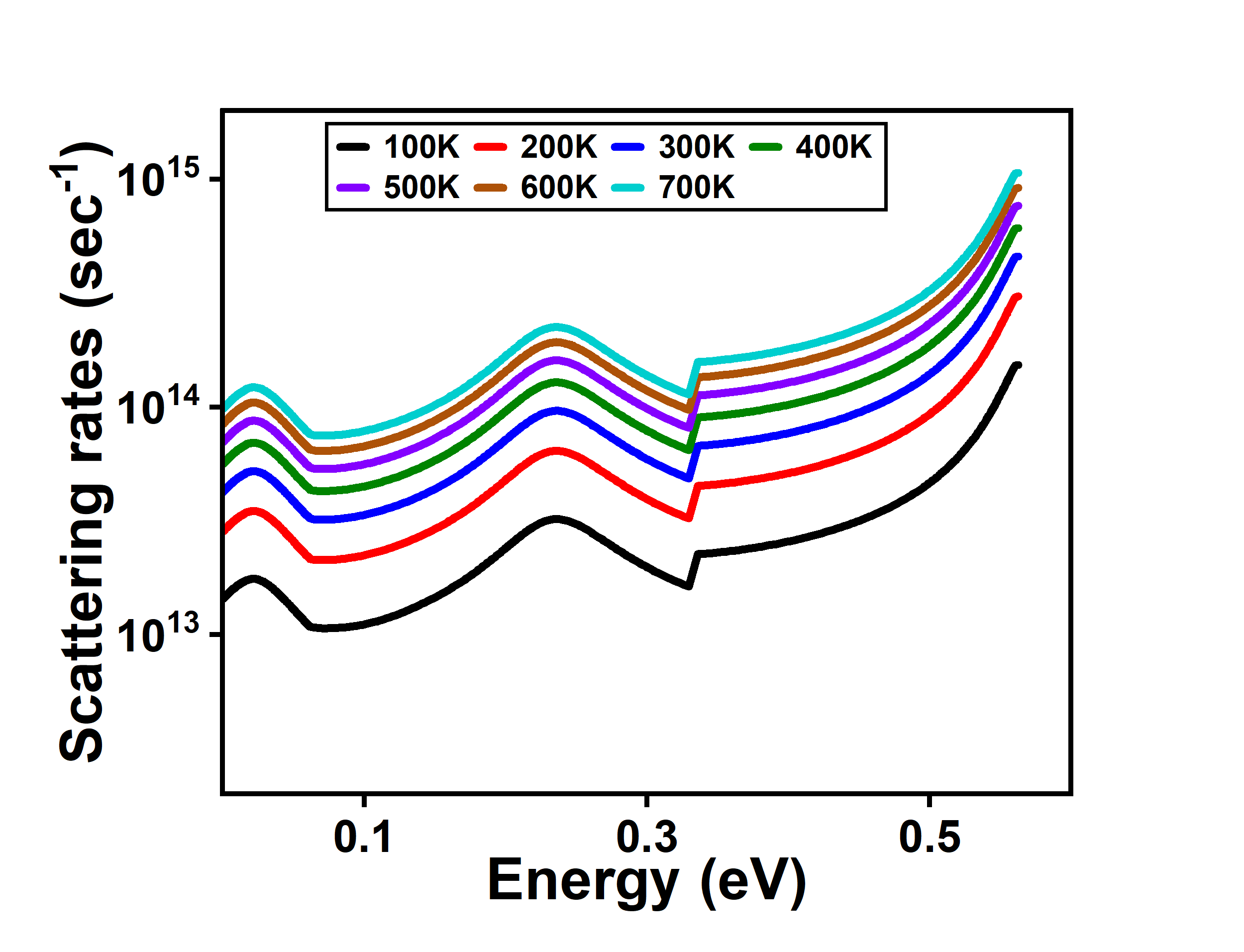
Fig. 1: Scattering rates vs. carrier energy at various temperatures with a doping concentration of $1\times 10^{12}\>cm^{-2}$.

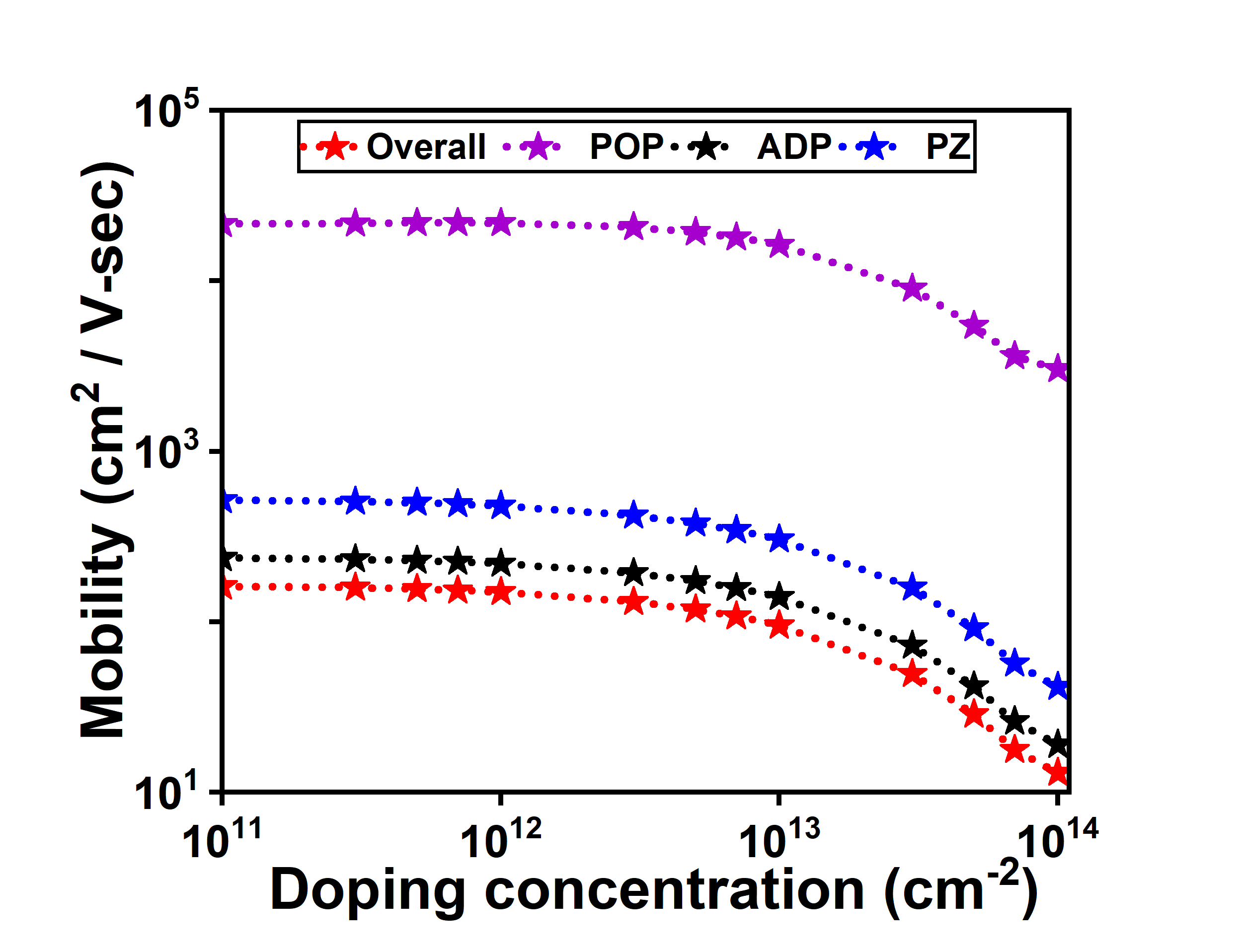
Fig. 2: Contribution to the mobility by different scattering mechanisms vs. doping concentration at room temperature with zero Hz frequency.

3.   Polar optical phonon scattering

The inelastic scattering in the system is caused by POP scattering mechanism. The POP scattering contribution to the out-scattering is given by Nag (2012); Kawamura and Sarma (1992)

$$\begin{split}S_{o}^{in}(k)=\frac{C_{{}_{POP}}}{(1-f_{0}(E))}[P+Q]\>,\end{split}$$ (15)

where

$$P=N_{V}(1-f_{0}(E+\hbar\omega_{{}_{POP}})I^{+}(E)\frac{k^{+}}{v(E+\hbar\omega_{{}_{POP}})}$$ (16)

$$\begin{split}Q=(N_{V}+1)(1-f_{0}(E-\hbar\omega_{{}_{POP}})\\ \times\leavevmode\nobreak\ I^{-}(E)\frac{k^{-}}{v(E-\hbar\omega_{{}_{POP}})}\end{split}$$ (17)

$$I^{+}(E)=\int_{0}^{2\pi}\frac{1}{q_{a}}d\theta$$ (18)

$$I^{-}(E)=\int_{0}^{2\pi}\frac{1}{q_{e}}d\theta$$ (19)

$$q_{a}=\left(k^{2}+\left(k^{+}\right)^{2}-2kk^{+}cos\>\theta\right)$$ (20)

$$q_{e}=\left(k^{2}+\left(k^{-}\right)^{2}-2kk^{-}cos\>\theta\right)\>,$$ (21)

where $k^{+}$ denotes the wave vector at energy $E+\hbar\>\omega$ and $k^{-}$ represents the wave vector at energy $E-\hbar\>\omega$. The angle between the initial wave vector k and the final wave vector $\textbf{k}^{{}^{\prime}}$ is defined as $\theta$.

$$C_{{}_{POP}}=\frac{e^{2}\omega_{{}_{POP}}}{8\pi\hbar\epsilon_{0}}\times\left(\frac{1}{\kappa_{{}_{\infty}}}-\frac{1}{\kappa_{{}_{0}}}\right)\>,$$ (22)

where $\kappa_{{}_{\infty}}$ and $\kappa_{{}_{0}}$ are the high and low-frequency dielectric constants, respectively.

The sum of in-scattering rates due to the POP absorption and the emission can be used to represent the in-scattering contribution due to the POP, an inelastic and anisotropic scattering mechanism.

$$S_{i}^{in}(k)=S_{a}^{in}(k)+S_{e}^{in}(k)\>,$$ (23)

where $S_{a}^{in}(k)$ denotes the in-scattering of electrons from energy $E-\hbar\>\omega_{{}_{POP}}$ to energy $E$ due to the absorption of polar optical phonons and $S_{e}^{in}(k)$ denotes the in-scattering of electrons from energy $E+\hbar\omega_{{}_{POP}}$ to energy $E$ due to the emission of polar optical phonons.

$$S_{a}^{in}(k)=C_{{}_{POP}}(N_{V}+1)f_{0}(E)J^{-}(E)\times A$$ (24)

$$A=\frac{k^{-}}{v(E-\hbar\>\omega_{{}_{POP}})f_{0}(E-\hbar\>\omega_{{}_{POP}})}$$ (25)

$$S_{e}^{in}(k)=C_{{}_{POP}}(N_{V})f_{0}(E)J^{+}(E)\times B$$ (26)

$$B=\frac{k^{+}}{v(E+\hbar\>\omega{{}_{{}_{POP}}})f_{0}(E+\hbar\>\omega_{{}_{{}_{POP}}})}$$ (27)

$$N_{V}=\frac{1}{exp(\hbar\>\omega_{{}_{POP}}/k_{B}T)-1}$$ (28)

$$J^{+}(E)=\int_{0}^{2\pi}\frac{cos\theta}{q_{{}_{i,e}}}d\theta$$ (29)

$$J^{-}(E)=\int_{0}^{2\pi}\frac{cos\theta}{q_{{}_{i,a}}}d\theta$$ (30)

$$q_{{}_{i,a}}=\Big{[}\left(k^{-}\right)^{2}+k^{2}-2kk^{-}cos\>\theta\Big{]}$$ (31)

$$q_{{}_{i,e}}=\Big{[}\left(k^{+}\right)^{2}+k^{2}-2kk^{+}cos\>\theta\Big{]}\>.$$ (32)

We replace the term $\frac{\hbar k}{m^{*}}$ by the group velocity Mandia et al. (2021, 2019) while deriving the expression for different scattering rates, which we calculate using the DFT band structure Mandia et al. (2019, 2021).

III Results and Discussion

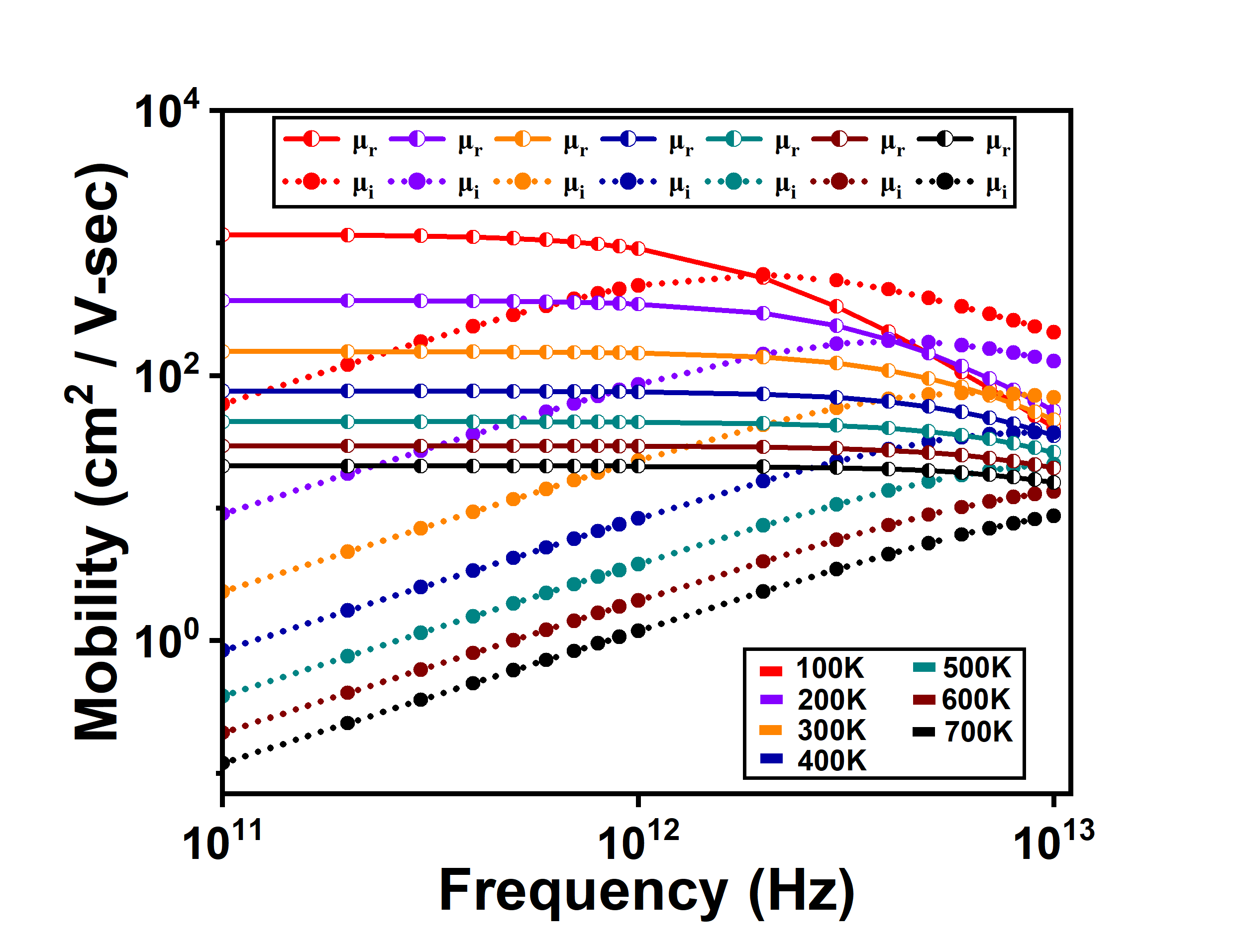
Fig. 3: Variation of the real and the imaginary components of mobility as a function of frequency for various temperatures with a doping concentration of $1\times 10^{12}\leavevmode\nobreak\ cm^{-2}$.

In Fig. 1, we show the total scattering rates, which is the sum of three scattering mechanisms we have considered in Ti₂CO₂. These three scattering mechanisms are the POP scattering, the PZ scattering, and the ADP scattering mechanisms. Scattering rates increase as we increase the temperature and hence the mobility decreases with an increase in the temperature.
In Fig. 2 we show the contribution to the mobility due to the ADP, the POP, and the PZ scattering mechanisms. Here, in Ti₂CO₂, the ADP scattering makes the most significant contribution followed by the PZ scattering mechanism and the POP scattering mechanism has the least effect. Therefore, the mobility and the conductivity in Ti₂CO₂ is mainly limited by the ADP scattering and hence acoustic phonons are the primary limiters of the conductivity and the mobility. Refer to our previous study Mandia et al. (2022) where we have computed the scattering rates due to the individual acoustic phonons for better understanding the nature of acoustic phonons that limit the conductivity in Ti₂CO₂.
In our previous study, we demonstrated that the longitudinal acoustic (LA) phonons play an important role in Ti₂CO₂. Therefore, the ADP and the PZ scattering are the two primary carrier scattering processes involved in Ti₂CO₂. As expected, the mobility decrease with increasing electron concentration. The mobility values are not significantly different for low electron concentrations, i.e., within the range [$1\times 10^{11}\leavevmode\nobreak\ cm^{-2}-1\times 10^{13}\leavevmode\nobreak\ cm^{-2}$]. However, there is a sharp reduction in the mobility, as shown in Fig. 2, at electron concentrations greater than $1\times 10^{13}\leavevmode\nobreak\ cm^{-2}$. Consider Matthiessen’s rule (33) to understand the mobility trend in relation to temperature and the carrier concentration, which can be expressed as

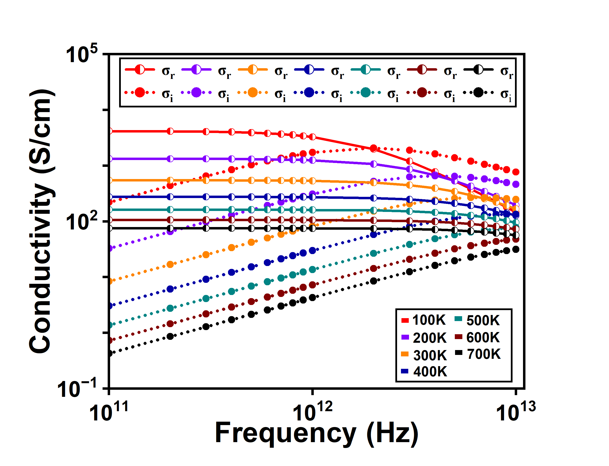
Fig. 4: Variation of the real and the imaginary components of conductivity as a function of frequency for various temperatures with a doping concentration of $1\times 10^{12}\leavevmode\nobreak\ cm^{-2}$.

$$\frac{1}{\mu}=\frac{1}{\mu_{{}_{ADP}}}+\frac{1}{\mu_{{}_{PZ}}}+\frac{1}{\mu_{{}_{POP}}}\>,$$ (33)

where $\mu$ stands for total mobility. Equation (33) states that the circumstance where the component with the lowest value is the most significant derives from the reciprocal relationship between the overall mobility and individual components. In Fig. 2, we show that the acoustic mode has the dominant contribution at all doping concentrations however, as demonstrated in Fig. 2, the PZ scattering mechanism significantly contributes across the entire doping range.

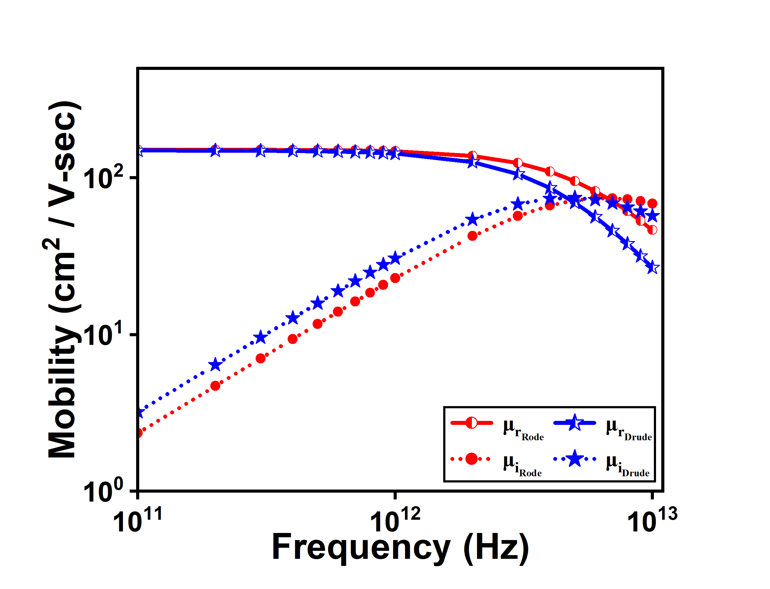
Fig. 5: Comparison of mobility (i.e., the real and the imaginary components) with the Rode’s and the Drude’s method at 300 K for doping concentration of $1\times 10^{12}\leavevmode\nobreak\ cm^{-2}$.

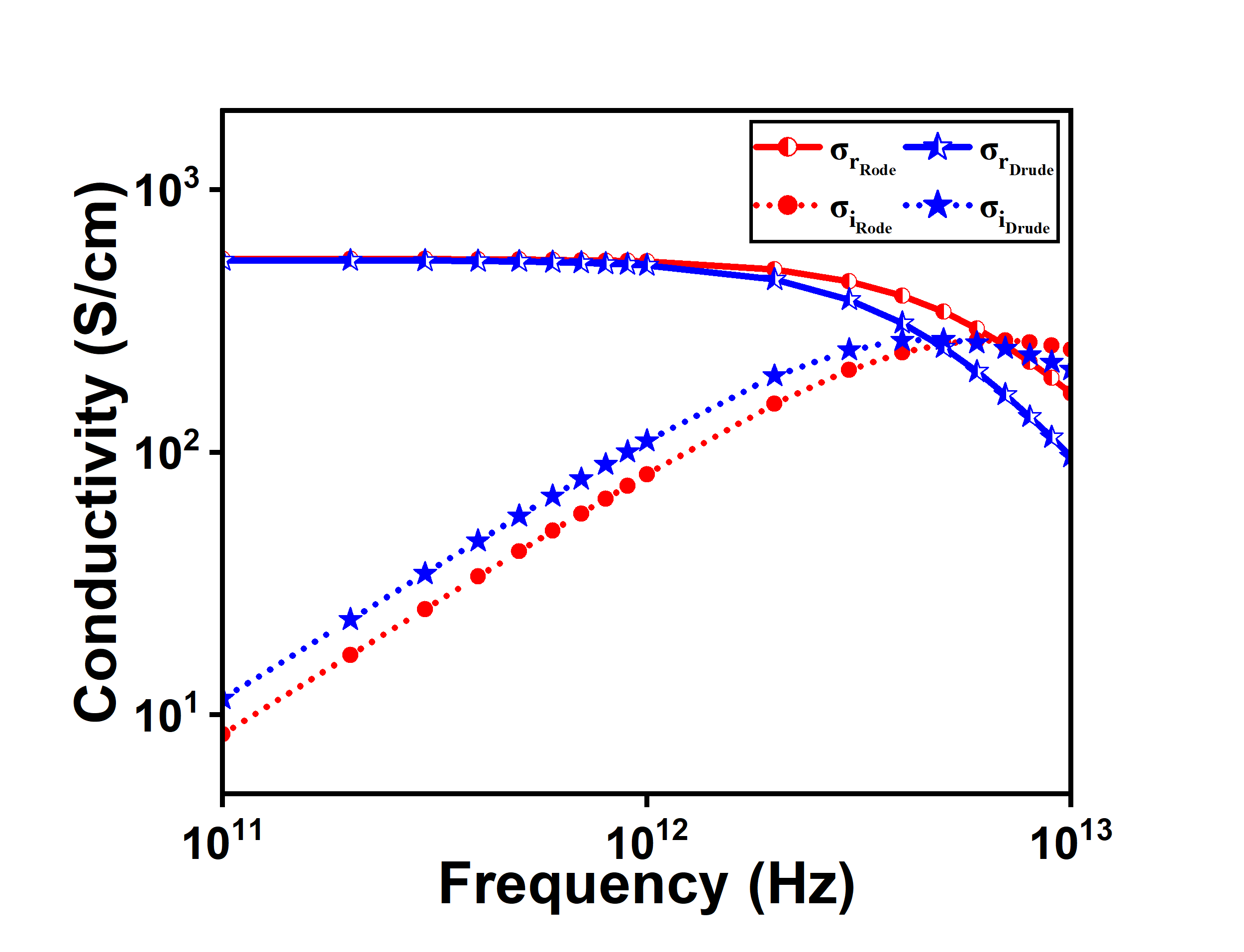
Fig. 6: Comparison of conductivity (i.e., the real and the imaginary components) with the Rode’s and the Drude’s method at 300 K for doping concentration of $1\times 10^{12}\leavevmode\nobreak\ cm^{-2}$.

In Fig. 3, we show that as the temperature rises from 100 K to 700 K, both $\mu_{r}$ and $\mu_{i}$ for $N_{D}=1\times 10^{12}\leavevmode\nobreak\ cm^{-2}$ decreases and these findings are explained by the fact that the scattering rate increases with increasing temperature. Figure 3 depicts the crossover between $\mu_{r}$ and $\mu_{i}$ at a specific frequency for each temperature, with the crossover shifting towards a higher frequency as the temperature increases. It is worth pointing that high-frequency effects are stronger at temperatures below the room temperature. Figure 4 shows the decrease in the conductivity caused by a reduction in mobility with an increase in temperature. In Fig. 5, we compare the mobility calculated using the Rode’s iterative method to the mobility calculated using the Drude’s theory. The Drude’s mobility can be expressed as Chattopadhyay (1980)

$$\mu_{r}=\frac{(e\tau/m^{*})}{(1+\omega^{2}\tau^{2})}$$ (34)

$$\mu_{i}=\frac{(e\omega\tau^{2}/m^{*})}{(1+\omega^{2}\tau^{2})}$$ (35)

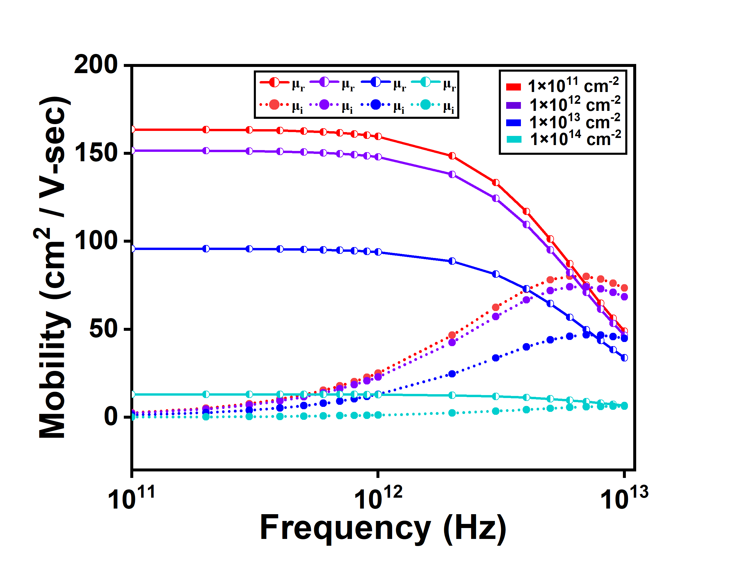
Fig. 7: Variation of the real and the imaginary components of the room temperature mobility as a function of frequency for various doping concentrations.

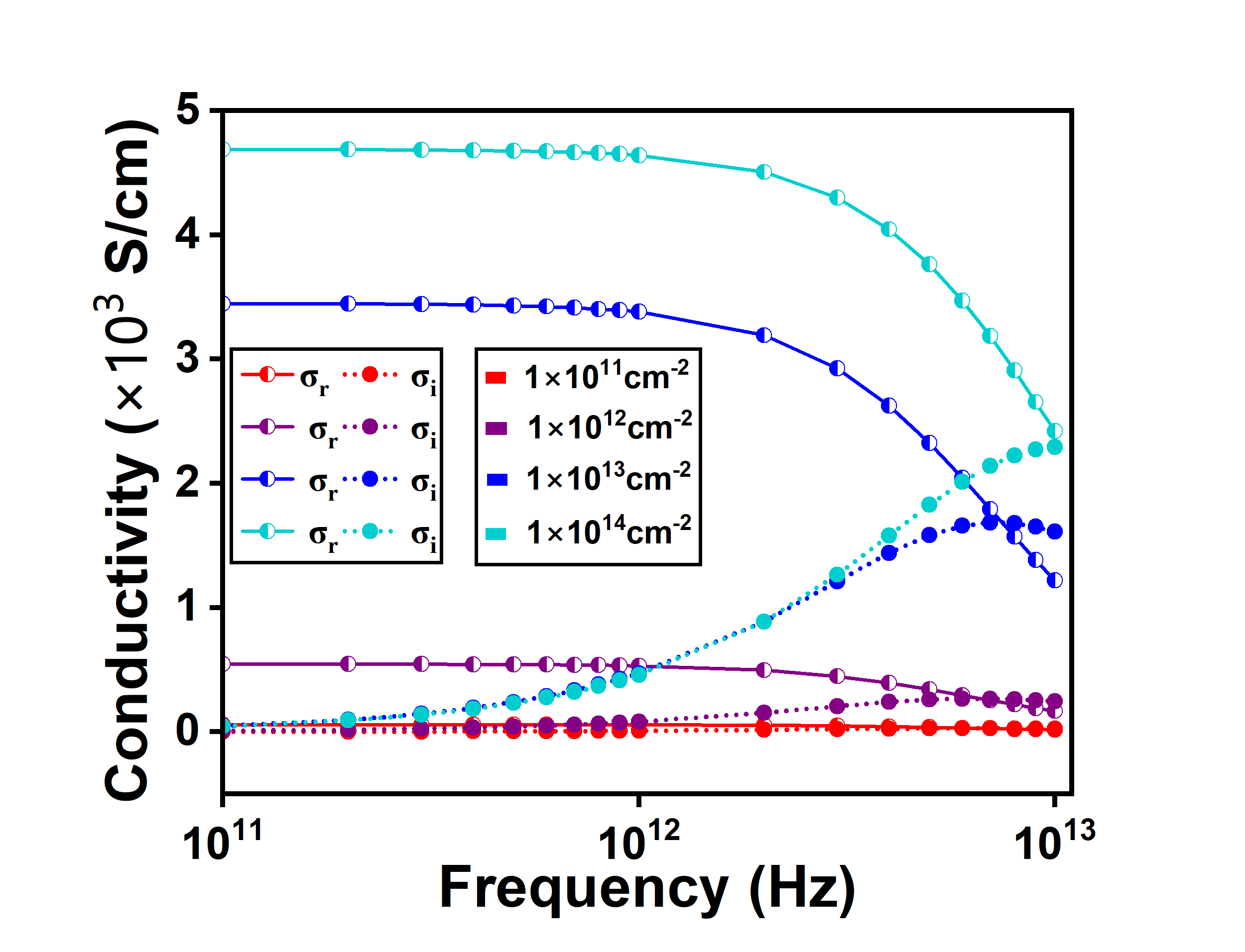
Fig. 8: Variation of the real and the imaginary components of conductivity as a function of frequency for various doping concentrations at room temperature.

Using the DFT, we calculate $m^{*}/m_{0}$, which is 0.4010, where $m_{0}$ is the rest mass of an electron. In order to determine the mobility using the Drude’s approach, we first determine $\tau$ value at $\omega=0$ using $\mu_{r}$ as $1.496985\times 10^{2}$ $cm^{2}/V-sec$, calculated at T =300 K and doping value of $1\times 10^{12}\leavevmode\nobreak\ cm^{-2}$. The calculated $\tau$ value is $3.4134\times 10^{-14}$ seconds. By adjusting the value of $\omega$ while keeping $\tau$ fixed at $3.4134\times 10^{-14}$ seconds, we calculate the real and the imaginary components of mobility.

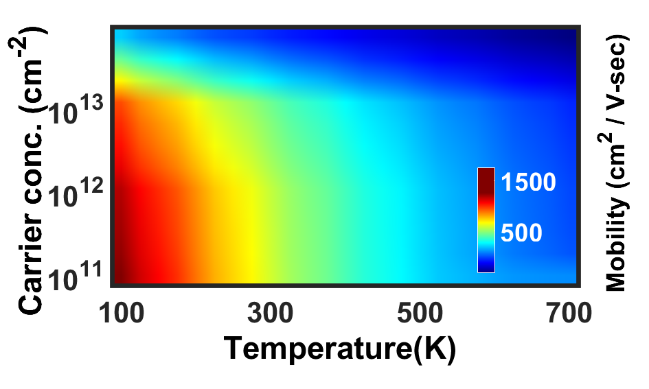
Fig. 9: Mobility vs. temperature and carrier concentration at 100 GHz frequency.

Figure 5 shows that the Drude’s values are close to exact values and that mobility can be estimated using the Drude’s model unless high accuracy is required. But at higher frequencies, there is a significant deviation in the real component of mobility, and the Rode’s method provides more accurate results. We also show the comparison of conductivity in Ti₂CO₂ calculated using the Rode’s and the Drude’s approach in a manner similar to that of the mobility. The calculation of Drude’s conductivity is straight forward using Eqs. (11) & (12). As shown in Fig. 6, Drude’s values for the real conductivity are relatively close to the exact values for the conductivity and hence the Drude’s method can be used to predict the mobility unless a high degree of accuracy is not required. At higher frequencies, a considerable variation has been seen, as a result the Rode’s approach is more faithful at higher frequencies.
In the Drude’s model, the effect of all scattering mechanisms is merged together in a single constant relaxation time. This simplification makes all the calculations easy however, this method has some disadvantages (i) $\tau$ is obtained by fitting the experimental results to the mobility, which limits the predictability of this model. (ii) Due to over simplification of scattering mechanisms, it may lead to inaccurate results. (iii) It does not provide any insight into which scattering mechanisms are playing the major role. Instead, we have calculated all required inputs from the DFT without relying on any experimental data, included all scattering mechanisms explicitly and provided an insight regarding which scattering mechanisms are physically relevant to the considered semiconductor. Hence, our approach can be used to predict the mobility and the conductivity of even new emerging materials accurately. This paves the way for researchers in designing semiconductors with highly accurate transport properties based on theoretical predictions.

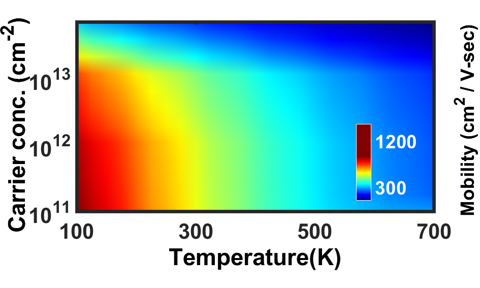
Fig. 10: Mobility vs. temperature and carrier concentration at 1 THz frequency.

Figure 7 shows that $\mu_{r}$ remains constant at room temperature up to a frequency of around 500 GHz. Beyond this frequency, $\mu_{r}$ falls while $\mu_{i}$ rises to a maximum and then falls. The simple Drude’s expressions easily predict this type of behavior. Figure 7 also shows that the mobility decreases as doping concentration increases. Figure 8 depicts the increase in the conductivity caused by an increase in carrier concentration. For low values of frequency, $\sigma_{r}$ and $\sigma_{i}$ are nearly constant whereas at higher frequencies, above $10^{12}$ Hz, $\sigma_{r}$ decreases significantly while $\sigma_{i}$ increases. Figures 9 and 10 depict the mobility vs. temperature and carrier concentration at frequencies of $100$ GHz and $1$ THz, respectively. It is clear from both the figures that the mobility decreases as the frequency value increases and mobility increases as the carrier concentration and temperature decrease.

IV Conclusion

In this work, we investigated using our recently developed $ab\leavevmode\nobreak\ initio$ transport model, the real and imaginary components of electron mobility and conductivity to conclusively depict carrier transport beyond the room temperature for frequency ranges upto the terahertz range. We also contrasted the carrier mobility and conductivity with respect to the Drude model to depict its inaccuracies for a meaningful comparison with experiments. Our calculations showed the effect of acoustic deformation potential scattering, piezoelectric scattering, and polar optical phonon scattering mechanisms. Without relying on experimental data, our model requires inputs calculated from first principles using density functional theory. Our results set the stage for providing ab-initio based ac- transport calculations given the current research on MXenes for high frequency applications.

Code Availability

The code used in this work is made available at https://github.com/anup12352/AMMCR.

References

- Mas-Balleste et al. (2011) R. Mas-Balleste, C. Gomez-Navarro, J. Gomez-Herrero, and F. Zamora, Nanoscale 3, 20 (2011).
- Novoselov et al. (2004) K. S. Novoselov, A. K. Geim, S. V. Morozov, D.-e. Jiang, Y. Zhang, S. V. Dubonos, I. V. Grigorieva, and A. A. Firsov, science 306, 666 (2004).
- Geim (2009) A. K. Geim, science 324, 1530 (2009).
- Geim and Novoselov (2010) A. K. Geim and K. S. Novoselov, in Nanoscience and technology: a collection of reviews from nature journals (World Scientific, 2010), pp. 11–19.
- Neto et al. (2009) A. C. Neto, F. Guinea, N. M. Peres, K. S. Novoselov, and A. K. Geim, Reviews of modern physics 81, 109 (2009).
- Novoselov et al. (2005) K. S. Novoselov, D. Jiang, F. Schedin, T. Booth, V. Khotkevich, S. Morozov, and A. K. Geim, Proceedings of the National Academy of Sciences 102, 10451 (2005).
- Akinwande et al. (2017) D. Akinwande, C. J. Brennan, J. S. Bunch, P. Egberts, J. R. Felts, H. Gao, R. Huang, J.-S. Kim, T. Li, Y. Li, et al., Extreme Mechanics Letters 13, 42 (2017).
- Cheng et al. (2019) J. Cheng, C. Wang, X. Zou, and L. Liao, Advanced Optical Materials 7, 1800441 (2019).
- Kim et al. (2015) S. J. Kim, K. Choi, B. Lee, Y. Kim, and B. H. Hong, Annual Review of Materials Research 45, 63 (2015).
- Wang and Song (2006) Z. L. Wang and J. Song, Science 312, 242 (2006).
- Lee et al. (2018) J. Lee, Z. Wang, K. He, R. Yang, J. Shan, and P. X.-L. Feng, Science advances 4, eaao6653 (2018).
- Cai et al. (2018) Y. Cai, J. Shen, G. Ge, Y. Zhang, W. Jin, W. Huang, J. Shao, J. Yang, and X. Dong, ACS nano 12, 56 (2018).
- Lin and Liu (2013) I.-T. Lin and J.-M. Liu, IEEE Journal of Selected Topics in Quantum Electronics 20, 122 (2013).
- Barsoum (2000) M. W. Barsoum, Progress in solid state chemistry 28, 201 (2000).
- Barsoum and Radovic (2011) M. W. Barsoum and M. Radovic, Annual review of materials research 41, 195 (2011).
- Naguib et al. (2011) M. Naguib, M. Kurtoglu, V. Presser, J. Lu, J. Niu, M. Heon, L. Hultman, Y. Gogotsi, and M. W. Barsoum, Advanced materials 23, 4248 (2011).
- Naguib et al. (2012a) M. Naguib, O. Mashtalir, J. Carle, V. Presser, J. Lu, L. Hultman, Y. Gogotsi, and M. W. Barsoum, ACS nano 6, 1322 (2012a).
- Naguib et al. (2014) M. Naguib, V. N. Mochalin, M. W. Barsoum, and Y. Gogotsi, Advanced materials 26, 992 (2014).
- Ghidiu et al. (2014) M. Ghidiu, M. Naguib, C. Shi, O. Mashtalir, L. Pan, B. Zhang, J. Yang, Y. Gogotsi, S. J. Billinge, and M. W. Barsoum, Chemical communications 50, 9517 (2014).
- Liang et al. (2015) X. Liang, A. Garsuch, and L. F. Nazar, Angewandte Chemie 127, 3979 (2015).
- Naguib et al. (2012b) M. Naguib, J. Come, B. Dyatkin, V. Presser, P.-L. Taberna, P. Simon, M. W. Barsoum, and Y. Gogotsi, Electrochemistry Communications 16, 61 (2012b).
- Tian et al. (2019) Y. Tian, Y. An, and J. Feng, ACS applied materials & interfaces 11, 10004 (2019).
- Xie et al. (2014) Y. Xie, M. Naguib, V. N. Mochalin, M. W. Barsoum, Y. Gogotsi, X. Yu, K.-W. Nam, X.-Q. Yang, A. I. Kolesnikov, and P. R. Kent, Journal of the American Chemical Society 136, 6385 (2014).
- Tang et al. (2012) Q. Tang, Z. Zhou, and P. Shen, Journal of the American Chemical Society 134, 16909 (2012).
- Er et al. (2014) D. Er, J. Li, M. Naguib, Y. Gogotsi, and V. B. Shenoy, ACS applied materials & interfaces 6, 11173 (2014).
- Halim et al. (2014) J. Halim, M. R. Lukatskaya, K. M. Cook, J. Lu, C. R. Smith, L.-Å. Näslund, S. J. May, L. Hultman, Y. Gogotsi, P. Eklund, et al., Chemistry of Materials 26, 2374 (2014).
- Hu et al. (2013) Q. Hu, D. Sun, Q. Wu, H. Wang, L. Wang, B. Liu, A. Zhou, and J. He, The Journal of Physical Chemistry A 117, 14253 (2013).
- Kumar et al. (2021) P. Kumar, S. Singh, S. Hashmi, and K.-H. Kim, Nano Energy 85, 105989 (2021).
- Lei et al. (2015) J.-C. Lei, X. Zhang, and Z. Zhou, Frontiers of Physics 10, 276 (2015).
- Li et al. (2018) X. Li, C. Wang, Y. Cao, and G. Wang, Chemistry–An Asian Journal 13, 2742 (2018).
- Hu et al. (2014) Q. Hu, H. Wang, Q. Wu, X. Ye, A. Zhou, D. Sun, L. Wang, B. Liu, and J. He, International journal of hydrogen energy 39, 10606 (2014).
- Wang et al. (2020) Y. Wang, Y. Xu, M. Hu, H. Ling, and X. Zhu, Nanophotonics 9, 1601 (2020).
- Jiang et al. (2020) X. Jiang, A. V. Kuklin, A. Baev, Y. Ge, H. Ågren, H. Zhang, and P. N. Prasad, Physics Reports 848, 1 (2020).
- Fu et al. (2021) B. Fu, J. Sun, C. Wang, C. Shang, L. Xu, J. Li, and H. Zhang, Small 17, 2006054 (2021).
- Xue et al. (2017) Q. Xue, H. Zhang, M. Zhu, Z. Pei, H. Li, Z. Wang, Y. Huang, Y. Huang, Q. Deng, J. Zhou, et al., Advanced Materials 29, 1604847 (2017).
- Xie et al. (2013) X. Xie, S. Chen, W. Ding, Y. Nie, and Z. Wei, Chemical Communications 49, 10112 (2013).
- Gandi et al. (2016) A. N. Gandi, H. N. Alshareef, and U. Schwingenschlögl, Chemistry of Materials 28, 1647 (2016).
- Zha et al. (2016) X.-H. Zha, Q. Huang, J. He, H. He, J. Zhai, J. S. Francisco, and S. Du, Scientific reports 6, 1 (2016).
- Sarikurt et al. (2018) S. Sarikurt, D. Çakır, M. Keçeli, and C. Sevik, Nanoscale 10, 8859 (2018).
- Kim and Alshareef (2019) H. Kim and H. N. Alshareef, ACS Materials Letters 2, 55 (2019).
- Sarycheva et al. (2018) A. Sarycheva, A. Polemi, Y. Liu, K. Dandekar, B. Anasori, and Y. Gogotsi, Science advances 4, eaau0920 (2018).
- Madsen and Singh (2006) G. K. Madsen and D. J. Singh, Computer Physics Communications 175, 67 (2006).
- Poncé et al. (2016) S. Poncé, E. R. Margine, C. Verdi, and F. Giustino, Computer Physics Communications 209, 116 (2016).
- Faghaninia et al. (2015) A. Faghaninia, J. W. Ager III, and C. S. Lo, Physical Review B 91, 235123 (2015).
- Ganose et al. (2021) A. M. Ganose, J. Park, A. Faghaninia, R. Woods-Robinson, K. A. Persson, and A. Jain, Nature communications 12, 1 (2021).
- Sindhu et al. (2022) B. Sindhu, V. Adepu, P. Sahatiya, and S. Nandi, FlatChem 33, 100367 (2022).
- Lee et al. (2021) S. Lee, E. H. Kim, S. Yu, H. Kim, C. Park, S. W. Lee, H. Han, W. Jin, K. Lee, C. E. Lee, et al., ACS nano 15, 8940 (2021).
- Ma et al. (2021) C. Ma, M.-G. Ma, C. Si, X.-X. Ji, and P. Wan, Advanced Functional Materials 31, 2009524 (2021).
- Zhang and Nicolosi (2019) C. J. Zhang and V. Nicolosi, Energy Storage Materials 16, 102 (2019).
- Pozar (2009) D. M. Pozar (2009).
- Iqbal et al. (2020) A. Iqbal, P. Sambyal, and C. M. Koo, Advanced Functional Materials 30, 2000883 (2020).
- Mandia et al. (2021) A. K. Mandia, B. Muralidharan, J.-H. Choi, S.-C. Lee, and S. Bhattacharjee, Computer Physics Communications 259, 107697 (2021).
- Rode (1970a) D. Rode, Physical Review B 2, 1012 (1970a).
- Rode (1973) D. Rode, physica status solidi (b) 55, 687 (1973).
- Rode (1975) D. Rode, in Semiconductors and semimetals (Elsevier, 1975), vol. 10, pp. 1–89.
- Lundstrom (2002) M. Lundstrom, Fundamentals of carrier transport (2002).
- Mandia et al. (2019) A. K. Mandia, R. Patnaik, B. Muralidharan, S.-C. Lee, and S. Bhattacharjee, Journal of Physics: Condensed Matter 31, 345901 (2019).
- Mandia et al. (2022) A. K. Mandia, N. A. Koshi, B. Muralidharan, S. C. Lee, and S. Bhattacharjee, Journal of Materials Chemistry C (2022).
- Kumar et al. (2023) R. Kumar, A. K. Mandia, A. Singh, and B. Muralidharan, arXiv preprint arXiv:2301.04858 (2023).
- Kresse and Furthmüller (1996a) G. Kresse and J. Furthmüller, Computational materials science 6, 15 (1996a).
- Kresse and Furthmüller (1996b) G. Kresse and J. Furthmüller, Physical Review B 54, 11169 (1996b).
- Blöchl (1994) P. E. Blöchl, Physical Review B 50, 17953 (1994).
- Kresse and Joubert (1999) G. Kresse and D. Joubert, Physical Review B 59, 1758 (1999).
- Perdew et al. (1996) J. P. Perdew, K. Burke, and M. Ernzerhof, Physical Review Letters 77, 3865 (1996).
- Rode (1970b) D. Rode, Physical Review B 2, 4036 (1970b).
- Ghosal et al. (1982) A. Ghosal, D. Chattopadhyay, and N. Purkait, physica status solidi (a) 73, K119 (1982).
- Nag (2012) B. R. Nag, Electron transport in compound semiconductors, vol. 11 (Springer Science & Business Media, 2012).
- Nag and Dutta (1975) B. Nag and G. Dutta, physica status solidi (b) 71, 401 (1975).
- Nag (1975) B. Nag, Journal of Applied Physics 46, 4819 (1975).
- Howarth and Sondheimer (1953) D. Howarth and E. H. Sondheimer, Proceedings of the Royal Society of London. Series A. Mathematical and Physical Sciences 219, 53 (1953).
- Hwang and Sarma (2008) E. Hwang and S. D. Sarma, Physical Review B 77, 115449 (2008).
- Lin et al. (2014) I.-T. Lin, Y.-P. Lai, K.-H. Wu, and J.-M. Liu, Applied Sciences 4, 28 (2014).
- Kaasbjerg et al. (2013) K. Kaasbjerg, K. S. Thygesen, and A.-P. Jauho, Physical Review B 87, 235312 (2013).
- Kawamura and Sarma (1992) T. Kawamura and S. D. Sarma, Physical review B 45, 3612 (1992).
- Chattopadhyay (1980) D. Chattopadhyay, Journal of Applied Physics 51, 1850 (1980).