fnets: An R Package for Network Estimation and Forecasting via Factor-Adjusted VAR Modelling

Abstract

The package fnets for the R language implements the suite of methodologies proposed by Barigozzi et al. (2022) for the network estimation and forecasting of high-dimensional time series under a factor-adjusted vector autoregressive model, which permits strong spatial and temporal correlations in the data. Additionally, we provide tools for visualising the networks underlying the time series data after adjusting for the presence of factors. The package also offers data-driven methods for selecting tuning parameters including the number of factors, order of autoregression and thresholds for estimating the edge sets of the networks of interest in time series analysis. We demonstrate various features of fnets on simulated datasets as well as real data on electricity prices.

Introduction

Vector autoregressive (VAR) models are popularly adopted for modelling time series datasets collected in many disciplines including economics (Koop, 2013), finance (Barigozzi and Brownlees, 2019), neuroscience (Kirch et al., 2015) and systems biology (Shojaie and Michailidis, 2010), to name a few. By fitting a VAR model to the data, we can infer dynamic interdependence between the variables and forecast future values. In particular, estimating the non-zero elements of the VAR parameter matrices recovers directed edges between the components of vector time series in a Granger causality network. Besides, by estimating the precision matrix (inverse of the covariance matrix) of the VAR innovations, we can define a network representing their contemporaneous dependencies by means of partial correlations. Finally, the inverse of the long-run covariance matrix of the data simultaneously captures lead-lag and contemporaneous co-movements of the variables. For further discussions on the network interpretation of VAR modelling, we refer to Dahlhaus (2000), Eichler (2007), Billio et al. (2012) and Barigozzi and Brownlees (2019).

Fitting VAR models to the data quickly becomes a high-dimensional problem as the number of parameters grows quadratically with the dimensionality of the data. There exists a mature literature on $\ell_{1}$-regularisation methods for estimating VAR models in high dimensions under suitable sparsity assumptions on the VAR parameters (Basu and Michailidis, 2015; Han et al., 2015; Kock and Callot, 2015; Medeiros and Mendes, 2016; Nicholson et al., 2020; Liu and Zhang, 2021). Consistency of such methods is derived under the assumption that the spectral density matrix of the data has bounded eigenvalues. However, in many applications, the datasets exhibit strong serial and cross-sectional correlations which leads to the violation of this assumption. As a motivating example, we introduce a dataset of node-specific prices in the PJM (Pennsylvania, New Jersey and Maryland) power pool area in the United States, see Energy price data for further details. Figure 1 demonstrates that the leading eigenvalue of the long-run covariance matrix (i.e. spectral density matrix at frequency $0$) increases linearly as the dimension of the data increases, which implies the presence of latent common factors in the panel data (Forni et al., 2000). Additionally, the left panel of Figure 2 shows the inadequacy of fitting a VAR model to such data under the sparsity assumption via $\ell_{1}$-regularisation methods, unless the presence of strong correlations is accounted for by a factor-adjustment step as in the right panel.

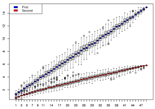
Figure 1: Box plots of the two largest eigenvalues ($y$-axis) of the long-run covariance matrix estimated from the energy price data collected between 01/01/2021 and 19/07/2021 ($n=200$), see Data example for further details. Cross-sections of the data are randomly sampled $100$ times for each given dimension $p\in\{2,\dots,50\}$ ($x$-axis) to produce the box plots.

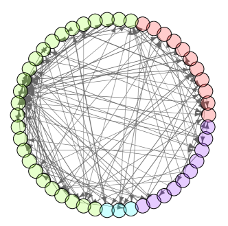
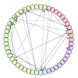
Figure 2: Granger causal networks defined in (5) obtained from fitting a VAR($1$) model to the energy price data analysed in Figure 1, without (left) and with (right) the factor adjustment step outlined in FNETS: Network estimation. Edge weights (proportional to the size of coefficient estimates) are visualised by the width of each edge, and the nodes are coloured according to their groupings, see Data example for further details.

Barigozzi et al. (2022) propose the FNETS methodology for factor-adjusted VAR modelling of high-dimensional, second-order stationary time series. Under their proposed model, the data is decomposed into two latent components such that the factor-driven component accounts for pervasive leading, lagging or contemporaneous co-movements of the variables, while the remaining idiosyncratic dynamic dependence between the variables is modelled by a sparse VAR process. Then, FNETS provides tools for inferring the networks underlying the latent VAR process and forecasting.

In this paper, we present an R package named fnets which implements the FNETS methodology. It provides a range of user-friendly tools for estimating and visualising the networks representing the interconnectedness of time series variables, and for producing forecasts. In addition, fnets thoroughly addresses the problem of selecting tuning parameters ranging from the number of factors and the VAR order, to regularisation and thresholding parameters adopted for producing sparse and interpretable networks. As such, a simple call of the main routine of fnets requires the input data only, and it outputs an object of S3 class fnets which is supported by a plot method for network visualisation and a predict method for time series forecasting.

There exist several packages for fitting VAR models and their extensions to high-dimensional time series, see lsvar (Bai, 2021), sparsevar (Vazzoler, 2021), nets (Brownlees, 2020), mgm (Haslbeck and Waldorp, 2020), graphicalVAR (Epskamp et al., 2018), bigVAR (Nicholson et al., 2017), and bigtime (Wilms et al., 2021). There also exist R packages for time series factor modelling such as dfms (Krantz and Bagdziunas, 2023) and sparseDFM (Mosley et al., 2023), and FAVAR (Bernanke et al., 2005) for Bayesian inference of factor-augmented VAR models. The package fnets is clearly distinguished from, and complements, the above list by handling strong cross-sectional and serial correlations in the data via factor-adjustment step performed in frequency domain. In addition, the FNETS methodology operates under the most general approach to high-dimensional time series factor modelling termed the Generalised Dynamic Factor (GDFM), first proposed in Forni et al. (2000) and further investigated in Forni et al. (2015). Accordingly, fnets is the first R package to provide tools for high-dimensional panel data analysis under the GDFM, such as fast computation of spectral density and autocovariance matrices via the Fast Fourier Transform, but it is flexible enough to allow for more restrictive static factor models. While there exist some packages for network-based time series modelling (e.g. GNAR, Knight et al., 2020), we highlight that the goal of fnets is to learn the networks underlying a time series and does not require a network as an input.

FNETS methodology

In this section, we introduce the factor-adjusted VAR model and describe the FNETS methodology proposed in Barigozzi et al. (2022) for network estimation and forecasting of high-dimensional time series. We limit ourselves to describing the key steps of FNETS and refer to the above paper for its comprehensive treatment, both methodologically and theoretically.

Factor-adjusted VAR model

A zero-mean, $p$-variate process $\bm{\xi}_{t}$ follows a VAR($d$) model if it satisfies

$$\bm{\xi}_{t} =\sum_{\ell=1}^{d}\mathbf{A}_{\ell}\bm{\xi}_{t-\ell}+\bm{\Gamma}^{1/2}\bm{\varepsilon}_{t},$$ (1)

where $\mathbf{A}_{\ell}\in R^{p\times p},\,1\leq\ell\leq d$, determine how future values of the series depend on their past. For the $p$-variate random vector $\bm{\varepsilon}_{t}=(\varepsilon_{1t},\ldots,\varepsilon_{pt})^{\top}$, we assume that $\varepsilon_{it}$ are independently and identically distributed (i.i.d.) for all $i$ and $t$ with $\mathop{\operator@font IE\hskip 0.13pt}(\varepsilon_{it})=0$ and $\mathsf{Var}(\varepsilon_{it})=1$. Then, the positive definite matrix $\bm{\Gamma}\in R^{p\times p}$ is the covariance matrix of the innovations $\bm{\Gamma}^{1/2}\bm{\varepsilon}_{t}$.

In the literature on factor modelling of high-dimensional time series, the factor-driven component exhibits strong cross-sectional and/or serial correlations by ‘loading’ finite-dimensional vectors of factors linearly. Among many time series factor models, the GDFM (Forni et al., 2000) provides the most general approach where the $p$-variate factor-driven component $\bm{\chi}_{t}$ admits the following representation

$$\bm{\chi}_{t} =\mathcal{B}(L)\mathbf{u}_{t}=\sum_{\ell=0}^{\infty}\mathbf{B}_{\ell}\mathbf{u}_{t-\ell}\text{ \ with \ }\mathbf{u}_{t}=(u_{1t},\ldots,u_{qt})^{\top}\text{ and }\mathbf{B}_{\ell}\in R^{p\times q},$$ (2)

for some fixed $q$, where $L$ stands for the lag operator. The $q$-variate random vector $\mathbf{u}_{t}$ contains the common factors which are loaded across the variables and time by the filter $\mathcal{B}(L)=\sum_{\ell=0}^{\infty}\mathbf{B}_{\ell}L^{\ell}$, and it is assumed that $u_{jt}$ are i.i.d. with $\mathop{\operator@font IE\hskip 0.13pt}(u_{jt})=0$ and $\mathsf{Var}(u_{jt})=1$. The model (2) reduces to a static factor model (Bai, 2003; Stock and Watson, 2002; Fan et al., 2013), when $\mathcal{B}(L)=\sum_{\ell=0}^{s}\mathbf{B}_{\ell}L^{\ell}$ for some finite integer $s\geq 0$. Then, we can write

$$\bm{\chi}_{t}=\bm{\Lambda}\mathbf{F}_{t}\text{ \ where \ }\mathbf{F}_{t}=(\mathbf{u}_{t}^{\top},\ldots,\mathbf{u}_{t-s}^{\top})^{\top}\text{ \ and \ }\bm{\Lambda}=[\mathbf{B}_{0},\ldots,\mathbf{B}_{s}]$$ (3)

with $r=q(s+1)$ as the dimension of static factors $\mathbf{F}_{t}$. Throughout, we refer to the models (2) and (3) as unrestricted and restricted to highlight that the latter imposes more restrictions on the model.

Barigozzi et al. (2022) propose a factor-adjusted VAR model under which we observe a zero-mean, second-order stationary process $\mathbf{X}_{t}=(X_{1t},\ldots,X_{pt})^{\top}$ for $t=1,\ldots,n$, that permits a decomposition into the sum of the unobserved components $\bm{\xi}_{t}$ and $\bm{\chi}_{t}$, i.e.

$$\mathbf{X}_{t}=\bm{\xi}_{t}+\bm{\chi}_{t}.$$ (4)

We assume that $\mathop{\operator@font IE\hskip 0.13pt}(\varepsilon_{it}u_{jt^{\prime}})=0$ for all $i$, $j$, $t$ and $t^{\prime}$ as is commonly assumed in the literature, such that $\mathop{\operator@font IE\hskip 0.13pt}(\xi_{it}\chi_{i^{\prime}t^{\prime}})=0$ for all $1\leq i,i^{\prime}\leq p$ and $t,t^{\prime}\in\mathbb{Z}$.

Networks

Under (4), it is of interest to infer three types of networks representing the interconnectedness of $\mathbf{X}_{t}$ after factor adjustment. Let $\mathcal{V}=\{1,\ldots,p\}$ denote the set of vertices representing the $p$ cross-sections. Then, the VAR parameter matrices, $\mathbf{A}_{\ell}=[A_{\ell,ii^{\prime}},\,1\leq i,i^{\prime}\leq p]$, encode the directed network $\mathcal{N}^{\text{{G}}}=(\mathcal{V},\mathcal{E}^{\text{{G}}})$ representing Granger causal linkages, where the set of edges are given by

$$\mathcal{E}^{\text{{G}}}=\left\{(i,i^{\prime})\in\mathcal{V}\times\mathcal{V}:\,A_{\ell,ii^{\prime}}\neq 0\text{ for some }1\leq\ell\leq d\right\}.$$ (5)

Here, the presence of an edge $(i,i^{\prime})\in\mathcal{E}^{\text{{G}}}$ indicates that $\xi_{i^{\prime},t-\ell}$ Granger causes $\xi_{it}$ at some lag $1\leq\ell\leq d$ (Dahlhaus, 2000).

The second network contains undirected edges representing contemporaneous cross-sectional dependence in VAR innovations $\bm{\Gamma}^{1/2}\bm{\varepsilon}_{t}$, denoted by $\mathcal{N}^{\text{{C}}}=(\mathcal{V},\mathcal{E}^{\text{{C}}})$. We have $(i,i^{\prime})\in\mathcal{E}^{\text{{C}}}$ if and only if the partial correlation between the $i$-th and $i^{\prime}$-th elements of $\bm{\Gamma}^{1/2}\bm{\varepsilon}_{t}$ is non-zero, which in turn is given by $-\delta_{ii^{\prime}}/\sqrt{\delta_{ii}\cdot\delta_{i^{\prime}i^{\prime}}}$ where $\bm{\Gamma}^{-1}=\bm{\Delta}=[\delta_{ii^{\prime}},\,1\leq i,i^{\prime}\leq p]$ (Peng et al., 2009). Hence, the set of edges for $\mathcal{N}^{\text{{C}}}$ is given by

$$\mathcal{E}^{\text{{C}}}=\left\{(i,i^{\prime})\in\mathcal{V}\times\mathcal{V}:\,i\neq i^{\prime}\text{ and }-\frac{\delta_{ii^{\prime}}}{\sqrt{\delta_{ii}\cdot\delta_{i^{\prime}i^{\prime}}}}\neq 0\right\},$$ (6)

Finally, we can summarise the aforementioned lead-lag and contemporaneous relations between the variables in a single, undirected network $\mathcal{N}^{\text{{L}}}=(\mathcal{V},\mathcal{E}^{\text{{L}}})$ by means of the long-run partial correlations of $\bm{\xi}_{t}$. Let $\bm{\Omega}=[\omega_{ii^{\prime}},\,1\leq i,i^{\prime}\leq p]$ denote the inverse of the zero-frequency spectral density (a.k.a. long-run covariance) of $\bm{\xi}_{t}$, which is given by $\bm{\Omega}=2\pi\mathcal{A}^{\top}(1)\bm{\Delta}\mathcal{A}(1)$ with $\mathcal{A}(z)=\mathbf{I}-\sum_{\ell=1}^{d}\mathbf{A}_{\ell}z^{\ell}$. Then, the long-run partial correlation between the $i$-th and $i^{\prime}$-th elements of $\bm{\xi}_{t}$, is obtained as $-\omega_{ii^{\prime}}/\sqrt{\omega_{ii}\cdot\omega_{i^{\prime}i^{\prime}}}$ (Dahlhaus, 2000), so the edge set of $\mathcal{N}^{\text{{L}}}$ is given by

$$\mathcal{E}^{\text{{L}}}=\left\{(i,i^{\prime})\in\mathcal{V}\times\mathcal{V}:\,i\neq i^{\prime}\text{ and }-\frac{\omega_{ii^{\prime}}}{\sqrt{\omega_{ii}\cdot\omega_{i^{\prime}i^{\prime}}}}\neq 0\right\}.$$ (7)

FNETS: Network estimation

We describe the three-step methodology for estimating the networks $\mathcal{N}^{\text{{G}}}$, $\mathcal{N}^{\text{{C}}}$ and $\mathcal{N}^{\text{{L}}}$. Throughout, we assume that the number of factors, either $q$ under the more general model in (2) or $r$ under the restricted model in (3), and the VAR order $d$ are known, and discuss its selection in Tuning parameter selection.

Step 1: Factor adjustment

The autocovariance (ACV) matrices of $\bm{\xi}_{t}$, denoted by $\bm{\Gamma}_{\xi}(\ell)=\mathop{\operator@font IE\hskip 0.13pt}(\bm{\xi}_{t-\ell}\bm{\xi}_{t}^{\top})$ for $\ell\geq 0$ and $\bm{\Gamma}_{\xi}(\ell)=(\bm{\Gamma}_{\xi}(-\ell))^{\top}$ for $\ell<0$, play a key role in network estimation. Since $\bm{\xi}_{t}$ is not directly observed, we propose to adjust for the presence of the factor-driven $\bm{\chi}_{t}$ and estimate $\bm{\Gamma}_{\xi}(\ell)$. For this, we adopt a frequency domain-based approach and perform dynamic principal component analysis (PCA). Spectral density matrix $\bm{\Sigma}_{x}(\omega)$ of a time series $\{\mathbf{X}_{t}\}_{t\in\mathbb{Z}}$ aggregates information of its ACV $\bm{\Gamma}_{x}(\ell),\,\ell\in\mathbb{Z}$, at a specific frequency $\omega\in[-\pi,\pi]$, and is obtained by the Fourier transform $\bm{\Sigma}_{x}(\omega)=(2\pi)^{-1}\sum_{\ell=-\infty}^{\infty}\bm{\Gamma}_{x}(\ell)\exp(-\iota\ell\omega)$ where $\iota=\sqrt{-1}$. Denoting the sample ACV matrix of $\mathbf{X}_{t}$ at lag $\ell$ by

$$\widehat{\bm{\Gamma}}_{x}(\ell)=\frac{1}{n}\sum_{t=\ell+1}^{n}\mathbf{X}_{t-\ell}\mathbf{X}_{t}^{\top}\text{ when }\ell\geq 0\quad\text{and}\quad\widehat{\bm{\Gamma}}_{x}(\ell)=(\widehat{\bm{\Gamma}}_{x}(-\ell))^{\top}\text{ when }\ell<0,$$

we estimate the spectral density of $\mathbf{X}_{t}$ by

$$\widehat{\bm{\Sigma}}_{x}(\omega_{k})=\frac{1}{2\pi}\sum_{\ell=-m}^{m}K\left(\frac{\ell}{m}\right)\widehat{\bm{\Gamma}}_{x}(\ell)\exp(-\iota\ell\omega_{k}),$$ (8)

where $K(\cdot)$ denotes a kernel, $m$ the kernel bandwidth (for its choice, see Tuning parameter selection) and $\omega_{k}=2\pi k/(2m+1)$ the Fourier frequencies. We adopt the Bartlett kernel as $K(\cdot)$ which ensures positive semi-definiteness of $\widehat{\bm{\Sigma}}_{x}(\omega)$ and also $\widehat{\bm{\Gamma}}_{\xi}(\ell)$ estimating $\bm{\Gamma}_{\xi}(\ell)$ obtained as described below.

Performing PCA on $\widehat{\bm{\Sigma}}_{x}(\omega_{k})$ at each $\omega_{k}$, we obtain the estimator of the spectral density matrix of $\bm{\chi}_{t}$ as $\widehat{\bm{\Sigma}}_{\chi}(\omega_{k})=\sum_{j=1}^{q}\widehat{\mu}_{x,j}(\omega_{k})\widehat{\mathbf{e}}_{x,j}(\omega_{k})(\widehat{\mathbf{e}}_{x,j}(\omega_{k}))^{*}$, where $\widehat{\mu}_{x,j}(\omega_{k})$ denotes the $j$-th largest eigenvalue of $\widehat{\bm{\Sigma}}_{x}(\omega_{k})$, $\widehat{\mathbf{e}}_{x,j}(\omega_{k})$ its associated eigenvector, and for any vector $\mathbf{a}\in\mathbb{C}^{n}$, we denote its transposed complex conjugate by $\mathbf{a}^{*}$. Then taking the inverse Fourier transform of $\widehat{\bm{\Sigma}}_{\chi}(\omega_{k}),\,-m\leq k\leq m$, leads to an estimator of $\bm{\Gamma}_{\chi}(\ell)$, the ACV matrix of $\bm{\chi}_{t}$, as

$$\widehat{\bm{\Gamma}}_{\chi}(\ell)=\frac{2\pi}{2m+1}\sum_{k=-m}^{m}\widehat{\bm{\Sigma}}_{\chi}(\omega_{k})\exp(\iota\ell\omega_{k})\quad\text{for \ }-m\leq\ell\leq m.$$

Finally, we estimate the ACV of $\bm{\xi}_{t}$ by

$$\widehat{\bm{\Gamma}}_{\xi}(\ell)=\widehat{\bm{\Gamma}}_{x}(\ell)-\widehat{\bm{\Gamma}}_{\chi}(\ell).$$ (9)

When we assume the restricted factor model in (3), the factor-adjustment step is simplified as it suffices to perform PCA in the time domain, i.e. eigenanalysis of the sample covariance matrix $\widehat{\bm{\Gamma}}_{x}(0)$. Denoting the eigenvector of $\widehat{\bm{\Gamma}}_{x}(0)$ associated with its $j$-th largest eigenvalue by $\widehat{\mathbf{e}}_{x,j}$, we obtain $\widehat{\bm{\Gamma}}_{\xi}(\ell)=\widehat{\bm{\Gamma}}_{x}(\ell)-\widehat{\mathbf{E}}_{x}\widehat{\mathbf{E}}_{x}^{\top}\widehat{\bm{\Gamma}}_{x}(\ell)\widehat{\mathbf{E}}_{x}\widehat{\mathbf{E}}_{x}^{\top}$ where $\widehat{\mathbf{E}}_{x}=[\widehat{\mathbf{e}}_{x,j},\,1\leq j\leq r]$.

Step 2: Estimation of $\mathcal{N}^{\text{{G}}}$

Recall from (5) that $\mathcal{N}^{\text{{G}}}$ representing Granger causal linkages, has its edge set determined by the VAR transition matrices $\mathbf{A}_{\ell},\,1\leq\ell\leq d$. By the Yule-Walker equation, we have $\bm{\beta}=[\mathbf{A}_{1},\dots,\mathbf{A}_{d}]^{\top}={\mathbf{G}(d)}^{-1}\mathbf{g}(d)$, where

$$\mathbf{G}(d)=\begin{bmatrix}\bm{\Gamma}_{\xi}(0)&\bm{\Gamma}_{\xi}(-1)&\ldots&\bm{\Gamma}_{\xi}(-d+1)\\ \bm{\Gamma}_{\xi}(1)&\bm{\Gamma}_{\xi}(0)&\ldots&\bm{\Gamma}_{\xi}(-d+2)\\ &&\ddots&\\ \bm{\Gamma}_{\xi}(d-1)&\bm{\Gamma}_{\xi}(d-2)&\ldots&\bm{\Gamma}_{\xi}(0)\end{bmatrix}\quad\text{and}\quad\mathbf{g}(d)=\begin{bmatrix}\bm{\Gamma}_{\xi}(1)\\ \bm{\Gamma}_{\xi}(2)\\ \vdots\\ \bm{\Gamma}_{\xi}(d)\end{bmatrix}.$$ (10)

We propose to estimate $\bm{\beta}$ as a regularised Yule-Walker estimator based on $\widehat{\mathbf{G}}(d)$ and $\widehat{\mathbf{g}}(d)$, each of which is obtained by replacing $\bm{\Gamma}_{\xi}(\ell)$ with $\widehat{\bm{\Gamma}}_{\xi}(\ell)$ (see (9)) in the definition of $\mathbf{G}(d)$ and $\mathbf{g}(d)$.

For any matrix $\mathbf{M}=[m_{ij}]\in R^{n_{1}\times n_{2}}$, let $|\mathbf{M}|_{1}=\sum_{i=1}^{n_{1}}\sum_{j=1}^{n_{2}}|m_{ij}|$, $|\mathbf{M}|_{\infty}=\max_{1\leq i\leq n_{1}}\max_{1\leq j\leq n_{2}}|m_{ij}|$ and $\mathsf{tr}(\mathbf{M})=\sum_{i=1}^{n_{1}}m_{ii}$ when $n_{1}=n_{2}$. We consider two estimators of $\bm{\beta}$. Firstly, we adopt a Lasso-type estimator which solves an $\ell_{1}$-regularised $M$-estimation problem

$$\widehat{\bm{\beta}}^{\text{{las}}}=\underset{\mathbf{M}\in\mathbb{R}^{pd\times p}}{\arg\min}\ \mathsf{tr}\left(\mathbf{M}^{\top}\widehat{\mathbf{G}}(d)\mathbf{M}-2\mathbf{M}^{\top}\widehat{\mathbf{g}}(d)\right)+\lambda|\mathbf{M}|_{1}$$ (11)

with a tuning parameter $\lambda>0$. In the implementation, we solve (11) via the fast iterative shrinkage-thresholding algorithm (FISTA, Beck and Teboulle, 2009). Alternatively, we adopt a constrained $\ell_{1}$-minimisation approach closely related to the Dantzig selector (DS, Candes and Tao, 2007):

$$\widehat{\bm{\beta}}^{\text{{DS}}}=\underset{\mathbf{M}\in\mathbb{R}^{pd\times p}}{\arg\min}\ |\mathbf{M}|_{1}\quad\text{subject to}\quad\left|\widehat{\mathbf{G}}(d)\mathbf{M}-\widehat{\mathbf{g}}(d)\right|_{\infty}\leq\lambda$$ (12)

for some tuning parameter $\lambda>0$. We divide (12) into $p$ sub-problems and obtain each column of $\widehat{\bm{\beta}}^{\text{{DS}}}$ via the simplex algorithm (using the function lp in lpSolve).

Barigozzi et al. (2022) establish the consistency of both $\widehat{\bm{\beta}}^{\text{{las}}}$ and $\widehat{\bm{\beta}}^{\text{{DS}}}$ but, as is typically the case for $\ell_{1}$-regularisation methods, they do not achieve exact recovery of the support of $\bm{\beta}$. Hence we propose to estimate the edge set of $\mathcal{N}^{\text{{G}}}$ by thresholding the elements of $\widehat{\bm{\beta}}$ with some threshold $\mathfrak{t}>0$, where either $\widehat{\bm{\beta}}=\widehat{\bm{\beta}}^{\text{{las}}}$ or $\widehat{\bm{\beta}}=\widehat{\bm{\beta}}^{\text{{DS}}}$, i.e.

$$\widetilde{\bm{\beta}}(\mathfrak{t}) =\begin{bmatrix}\widehat{\beta}_{ij}\cdot\mathbb{I}_{\{|\widehat{\beta}_{ij}|>\mathfrak{t}\}},\,1\leq i\leq pd,\,1\leq j\leq p\end{bmatrix}.$$ (13)

We discuss cross validation and information criterion methods for selecting $\lambda$, and a data-driven choice of $\mathfrak{t}$, in Tuning parameter selection.

Step 3: Estimation of $\mathcal{N}^{\text{{C}}}$ and $\mathcal{N}^{\text{{L}}}$

From the definitions of $\mathcal{N}^{\text{{C}}}$ and $\mathcal{N}^{\text{{L}}}$ given in (6) and (7), their edge sets are obtained by estimating $\bm{\Delta}=\bm{\Gamma}^{-1}$ and $\bm{\Omega}=2\pi\mathcal{A}^{\top}(1)\bm{\Delta}\mathcal{A}(1)$. Given $\widehat{\bm{\beta}}=[\widehat{\mathbf{A}}_{1},\ldots,\widehat{\mathbf{A}}_{d}]^{\top}$, some estimator of the VAR parameter matrices obtained as in either (11) or (12), a natural estimator of $\bm{\Gamma}$ arises from the Yule-Walker equation $\bm{\Gamma}=\bm{\Gamma}_{\xi}(0)-\sum_{\ell=1}^{d}\mathbf{A}_{\ell}\bm{\Gamma}_{\xi}(\ell)=\bm{\Gamma}_{\xi}(0)-\bm{\beta}^{\top}{\mathbf{g}}$, as $\widehat{\bm{\Gamma}}=\widehat{\bm{\Gamma}}_{\xi}(0)-\widehat{\bm{\beta}}^{\top}\widehat{\mathbf{g}}$. In high dimensions, it is not feasible or recommended to directly invert $\widehat{\bm{\Gamma}}$ to estimate $\bm{\Delta}$. Therefore, we adopt a constrained $\ell_{1}$-minimisation method motivated by the CLIME methodology of Cai et al. (2011).

Specifically, the CLIME estimator of $\bm{\Delta}$ is obtained by first solving

$$\check{\bm{\Delta}} ={\arg\min}_{\mathbf{M}\in\mathbb{R}^{p\times p}}|\mathbf{M}|_{1}\quad\text{subject to}\quad\left|\widehat{\bm{\Gamma}}\mathbf{M}-\mathbf{I}\right|_{\infty}\leq\eta,$$ (14)

and applying a symmetrisation step to $\check{\bm{\Delta}}=[\check{\delta}_{ii^{\prime}},\,1\leq i,j\leq p]$ as

$$\widehat{\bm{\Delta}} =[\widehat{\delta}_{ii^{\prime}},\,1\leq i,i^{\prime}\leq p]\text{ with }\widehat{\delta}_{ii^{\prime}}=\check{\delta}_{ii^{\prime}}\cdot\mathbb{I}_{\{|\check{\delta}_{ii^{\prime}}|\leq|\check{\delta}_{i^{\prime}i}|\}}+\check{\delta}_{i^{\prime}i}\cdot\mathbb{I}_{\{|\check{\delta}_{i^{\prime}i}|<|\check{\delta}_{ii^{\prime}}|\}}.$$ (15)

for some tuning parameter $\eta>0$. Cai et al. (2016) propose ACLIME, which improves the CLIME estimator by selecting the parameter $\eta$ in (15) adaptively. It first produces the estimators of the diagonal entries $\delta_{ii},1\leq i\leq p$, as in (15) with $\eta_{1}=2\sqrt{\log(p)/n}$ as the tuning parameter. Then these estimates are used for adaptive tuning parameter selection in the second step. We provide the full description of the ACLIME estimator along with the details of its implementation in ACLIME estimator of the Appendix.

Given the estimators $\widehat{\mathcal{A}}(1)=\mathbf{I}-\sum_{\ell=1}^{d}\widehat{\mathbf{A}}_{\ell}$ and $\widehat{\bm{\Delta}}$, we estimate $\bm{\Omega}$ by $\widehat{\bm{\Omega}}=2\pi\widehat{\mathcal{A}}^{\top}(1)\widehat{\bm{\Delta}}\widehat{\mathcal{A}}(1)$. In Barigozzi et al. (2022), $\widehat{\bm{\Delta}}$ and $\widehat{\bm{\Omega}}$ are shown to be consistent in $\ell_{\infty}$- and $\ell_{1}$-norms under suitable sparsity assumptions. However, an additional thresholding step as in (13) is required to guarantee consistency in estimating the support of $\bm{\Delta}$ and $\bm{\Omega}$ and consequently the edge sets of $\mathcal{N}^{\text{{C}}}$ and $\mathcal{N}^{\text{{L}}}$. We discuss data-driven selection of these thresholds and $\eta$ in Tuning parameter selection.

FNETS: Forecasting

Following the estimation procedure, FNETS performs forecasting by estimating the best linear predictor of $\mathbf{X}_{n+a}$ given $\mathbf{X}_{t},\,t\leq n$, for a fixed integer $a\geq 1$. This is achieved by separately producing the best linear predictors of $\bm{\chi}_{n+a}$ and $\bm{\xi}_{n+a}$ as described below, and then combining them.

Forecasting the factor-driven component

For given $a\geq 0$, the best linear predictor of $\bm{\chi}_{n+a}$ given $\mathbf{X}_{t},\,t\leq n$, under (2) is

$$\bm{\chi}_{n+a|n}=\sum_{\ell=0}^{\infty}\mathbf{B}_{\ell+a}\mathbf{u}_{n-\ell}.$$

Forni et al. (2015) show that the model (2) admits a low-rank VAR representation with $\mathbf{u}_{t}$ as the innovations under mild conditions, and Forni et al. (2017) propose the estimators of $\mathbf{B}_{\ell}$ and $\mathbf{u}_{t}$ based on this representation which make use of the estimators of the ACV of $\bm{\chi}_{t}$ obtained as described in Step 1. Then, a natural estimator of $\bm{\chi}_{n+a|n}$ is

$$\widehat{\bm{\chi}}^{\text{{unr}}}_{n+a|n}=\sum_{\ell=0}^{K}\widehat{\mathbf{B}}_{\ell+a}\widehat{\mathbf{u}}_{n-\ell}$$ (16)

for some truncation lag $K$. We refer to $\widehat{\bm{\chi}}^{\text{{unr}}}_{n+a|n}$ as the unrestricted estimator of $\bm{\chi}_{n+a|n}$ as it is obtained without imposing any restrictions on the factor model (2).

When $\bm{\chi}_{t}$ admits the static representation in (3), we can show that $\bm{\chi}_{n+a|n}=\bm{\Gamma}_{\chi}(-a)\mathbf{E}_{\chi}\bm{\mathcal{M}}_{\chi}^{-1}\mathbf{E}_{\chi}^{\top}\bm{\chi}_{n}$, where $\bm{\mathcal{M}}_{\chi}\in R^{r\times r}$ is a diagonal matrix with the $r$ eigenvalues of $\bm{\Gamma}_{\chi}(0)$ on its diagonal and $\mathbf{E}_{\chi}\in R^{p\times r}$ the matrix of the corresponding eigenvectors; see Section 4.1 of Barigozzi et al. (2022) and also Forni et al. (2005). This suggests an estimator

$$\widehat{\bm{\chi}}^{\text{{res}}}_{n+a|n}=\widehat{\bm{\Gamma}}_{\chi}(-a)\widehat{\mathbf{E}}_{\chi}\widehat{\bm{\mathcal{M}}}_{\chi}^{-1}\widehat{\mathbf{E}}_{\chi}^{\top}\mathbf{X}_{n},$$ (17)

where $\widehat{\bm{\mathcal{M}}}_{\chi}$ and $\widehat{\mathbf{E}}_{\chi}$ are obtained from the eigendecomposition of $\widehat{\bm{\Gamma}}_{\chi}(0)$. We refer to $\widehat{\bm{\chi}}^{\text{{res}}}_{n+a|n}$ as the restricted estimator of $\bm{\chi}_{n+a|n}$. As a by-product, we obtain the in-sample estimators of $\bm{\chi}_{t},\,t\leq n$, as $\widehat{\bm{\chi}}_{t|n}=\widehat{\bm{\chi}}_{t}$, with either of the two estimators in (16) and (17).

Forecasting the latent VAR process

Once the VAR parameters are estimated either as in (11) or (12), we produce an estimator of $\bm{\xi}_{n+a|n}=\sum_{\ell=1}^{d}\mathbf{A}_{\ell}\bm{\xi}_{n+a-\ell}$, the best linear predictor of $\bm{\xi}_{n+a}$ given $\mathbf{X}_{t},\,t\leq n$, as

$$\widehat{\bm{\xi}}_{n+a|n}=\sum_{\ell=1}^{\max(1,a)-1}\widehat{\mathbf{A}}_{\ell}\widehat{\bm{\xi}}_{n+a-\ell|n}+\sum_{\ell=\max(1,a)}^{d}\widehat{\mathbf{A}}_{\ell}\widehat{\bm{\xi}}_{n+a-\ell}.$$ (18)

Here, $\widehat{\bm{\xi}}_{n+1-\ell}=\mathbf{X}_{n+1-\ell}-\widehat{\bm{\chi}}_{n+1-\ell}$ denotes the in-sample estimator of $\bm{\xi}_{n+1-\ell}$, which may be obtained with either of the two (in-sample) estimators of the factor-driven component in (16) and (17).

Tuning parameter selection

Factor numbers $q$ and $r$

The estimation and forecasting tools of the FNETS methodology require the selection of the number of factors, i.e. $q$ under the unrestricted factor model in (2), and $r$ under the restricted, static factor model in (3). Under (2), there exists a large gap between the $q$ leading eigenvalues of the spectral density matrix of $\mathbf{X}_{t}$ and the remainder which diverges with $p$ (see also Figure 1 We provide two methods for selecting the factor number $q$, which make use of the postulated eigengap using $\widehat{\mu}_{x,j}(\omega_{k}),\,1\leq j\leq p$, the eigenvalues of the spectral density estimator of $\mathbf{X}_{t}$ in (8) at a given Fourier frequency $\omega_{k},\,-m\leq k\leq m$.

Hallin and Liška (2007) propose an information criterion for selecting the number of factors under the model (2) and further, a methodology for tuning the multiplicative constant in the penalty. Define

$$\text{IC}(b,c)=\log\left(\frac{1}{p}\sum_{j=b+1}^{p}\frac{1}{2m+1}\sum_{k=-m}^{m}\widehat{\mu}_{x,j}(\omega_{k})\right)+b\cdot c\cdot\text{pen}(n,p),$$ (19)

where $\text{pen}(n,p)=\min(p,m^{2},\sqrt{n/m})^{-1/2}$ by default (for other choices of the information criterion, see Appendix A) and $c>0$ a constant. Provided that $\text{pen}(n,p)\to 0$ sufficiently slowly, for an arbitrary value of $c$, the factor number $q$ is consistently estimated by the minimiser of $\text{IC}(b,c)$ over $b\in\{0,\ldots,\bar{q}\}$, with some fixed $\bar{q}$ as the maximum allowable number of factors. However, this is not the case in finite sample, and Hallin and Liška (2007) propose to simultaneously select $q$ and $c$. First, we identify $\widehat{q}(n_{l},p_{l},c)=\arg\min_{0\leq b\leq\bar{q}}\text{IC}(n_{l},p_{l},b,c)$ where $\text{IC}(n_{l},p_{l},b,c)$ is constructed analogously to $\text{IC}(b,c)$, except that it only involves the sub-sample $\{X_{it},\,1\leq i\leq p_{l},\,1\leq t\leq n_{l}\}$, for sequences $0<n_{1}<\ldots<n_{L}=n$ and $0<p_{1}<\ldots<p_{L}=p$. Then, denoting the sample variance of $\widehat{q}(n_{l},p_{l},c),\,1\leq l\leq L$, by $S(c)$, we select $\widehat{q}=\widehat{q}(n,p,\widehat{c})$ with $\widehat{c}$ corresponding to the second interval of stability with $S(c)=0$ for the mapping $c\mapsto S(c)$ as $c$ increases from $0$ to some $c_{\max}$ (the first stable interval is where $\bar{q}$ is selected with a very small value of $c$). Figure 3 plots $\widehat{q}(n,p,c)$ and $S(c)$ for varying values of $c$ obtained from a dataset simulated in Data generation. In the implementation of this methodology, we set $n_{l}=n-(L-l)\lfloor n/20\rfloor$ and $p_{l}=\lfloor 3p/4+lp/40\rfloor$ with $L=10$, and $\bar{q}=\min(50,\lfloor\sqrt{\min(n-1,p)}\rfloor)$.

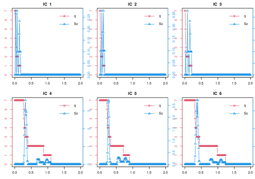
Figure 3: Plots of $c$ against $\widehat{q}(n,p,c)$ (in circle, $y$-axis on the left) and $S(c)$ (in triangle, $y$-axis on the right) with the six IC (see Appendix A) implemented in the function factor.number of fnets, on a dataset simulated as in Data generation (with $n=500$, $p=50$ and $q=2$). With the default choice of IC in (19) (IC₅), we obtain $\widehat{q}=\widehat{q}(n,p,\widehat{c})=2$ correctly estimating $q=2$.

Alternatively, we can adopt the ratio-based estimator $\widehat{q}=\arg\min_{1\leq b\leq\bar{q}}\text{ER}(b)$ proposed in Avarucci et al. (2022), where

$$\text{ER}(b)=\left(\sum_{k=-m}^{m}\widehat{\mu}_{x,b+1}(\omega_{k})\right)^{-1}\left(\sum_{k=-m}^{m}\widehat{\mu}_{x,b}(\omega_{k})\right).$$ (20)

These methods are readily modified to select the number of factors $r$ under the restricted factor model in (3), by replacing $(2m+1)^{-1}\sum_{k=-m}^{m}\widehat{\mu}_{x,j}(\omega_{k})$ with $\widehat{\mu}_{x,j}$, the $j$-th largest eigenvalues of the sample covariance matrix $\widehat{\bm{\Gamma}}_{x}(0)$. We refer to Bai and Ng (2002) and Alessi et al. (2010) for the discussion of the information criterion-based method in this setting, and Ahn and Horenstein (2013) for that of the eigenvalue ratio-based method.

Threshold $\mathfrak{t}$

Motivated by Liu et al. (2021), we propose a method for data-driven selection of the threshold $\mathfrak{t}$, which is applied to the estimators of $\mathbf{A}_{\ell},\,1\leq\ell\leq d$, $\bm{\Delta}$ or $\bm{\Omega}$ for estimating the edge sets of $\mathcal{N}^{\text{{G}}}$, $\mathcal{N}^{\text{{C}}}$ or $\mathcal{N}^{\text{{L}}}$, respectively; see also (13).

Let $\mathbf{B}=[b_{ij}]\in R^{m\times n}$ denote a matrix for which a threshold is to be selected, i.e. $\mathbf{B}$ may be either $\widehat{\bm{\beta}}=[\widehat{\mathbf{A}}_{1},\ldots,\widehat{\mathbf{A}}_{d}]^{\top}$, $\widehat{\bm{\Delta}}_{0}$ ($\widehat{\bm{\Delta}}$ with diagonals set to zero) or $\widehat{\bm{\Omega}}_{0}$ ($\widehat{\bm{\Omega}}$ with diagonals set to zero) obtained from Steps 2 and 3 of FNETS. We work with $\widehat{\bm{\Delta}}_{0}$ and $\widehat{\bm{\Omega}}_{0}$ since we do not threshold the diagonal entries of $\widehat{\bm{\Delta}}$ and $\widehat{\bm{\Omega}}$. As such estimators have been shown to achieve consistency in $\ell_{\infty}$-norm, we expect there exists a large gap between the entries of $\mathbf{B}$ corresponding to true positives and false positives. Further, it is expected that the number of edges reduces at a faster rate when increasing the threshold from $0$ towards this (unknown) gap, compared to when increasing the threshold from the gap to $|\mathbf{B}|_{\infty}$. Therefore, we propose to identify this gap by casting the problem as that of locating a single change point in the trend of the ratio of edges to non-edges,

$$\text{Ratio}_{k}=\frac{|\mathbf{B}(\mathfrak{t}_{k})|_{0}}{\max(N-|\mathbf{B}(\mathfrak{t}_{k})|_{0},1)},\quad k=1,\dots,M.$$

Here, $\mathbf{B}(\mathfrak{t})=[b_{ij}\cdot\mathbb{I}_{\{|b_{ij}|>\mathfrak{t}\}}]$, $|\mathbf{B}(\mathfrak{t})|_{0}=\sum_{i=1}^{m_{1}}\sum_{j=1}^{m_{2}}\mathbb{I}_{\{|b_{ij}|>\mathfrak{t}\}}$ and $\{\mathfrak{t}_{k},\,1\leq k\leq M:\,0=\mathfrak{t}_{1}<\mathfrak{t}_{2}<\dots<\mathfrak{t}_{M}=|\mathbf{B}|_{\infty}\}$ denotes a sequence of candidate threshold values. We recommend using an exponentially growing sequence for $\{\mathfrak{t}_{k}\}_{k=1}^{M}$ since the size of the false positive entries tends to be very small. The quantity $N$ in the denominator of Ratio_k is set as $N=p^{2}d$ when $\mathbf{B}=\widehat{\bm{\beta}}$, and $N=p(p-1)$ when $\mathbf{B}=\widehat{\bm{\Delta}}_{0}$ or $\mathbf{B}=\widehat{\bm{\Omega}}_{0}$. Then, from the difference quotient

$$\text{Diff}_{k}=\frac{\text{Ratio}_{k}-\text{Ratio}_{k-1}}{\mathfrak{t}_{k}-\mathfrak{t}_{k-1}},\quad k=2,\ldots,M,$$

we compute the cumulative sum (CUSUM) statistic

$$\text{CUSUM}_{k}=\sqrt{\frac{k(M-k)}{M}}\left|\frac{1}{k}\sum_{l=2}^{k}\text{Diff}_{l}-\frac{1}{M-k}\sum_{l=k+1}^{M}\text{Diff}_{l}\right|,\quad k=2,\ldots,M-1,$$

and select $\mathfrak{t}_{\text{ada}}=\mathfrak{t}_{k^{*}}$ with $k^{*}={\arg\max}_{2\leq k\leq M-1}\text{CUSUM}_{k}$. For illustration, Figure 4 plots Ratio_k and CUSUM_k against candidate thresholds for the dataset simulated in Data generation.

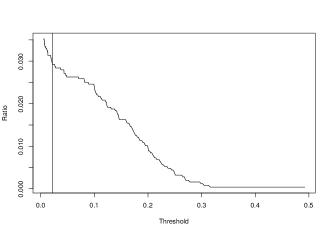
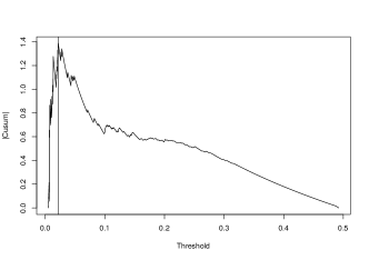
Figure 4: Ratio_k (left) and CUSUM_k (right) plotted against $\mathfrak{t}_{k}$ when $\mathbf{B}=\widehat{\bm{\beta}}^{\text{{las}}}$ obtained from the data simulated in Data generation with $n=500$ and $p=50$, as a Lasso estimator of the VAR parameter matrix, with the selected $\mathfrak{t}_{\text{ada}}$ denoted by the vertical lines.

VAR order $d$, $\lambda$ and $\eta$

Step 2 and Step 3 of the network estimation methodology of FNETS involve the selection of the tuning parameters $\lambda$ and $\eta$ (see (11), (12) and (14)) and the VAR order $d$. While there exist a variety of methods available for VAR order selection in fixed dimensions (Lütkepohl, 2005, Chapter 4), the data-driven selection of $d$ in high dimensions remains largely unaddressed with a few exceptions (Nicholson et al., 2020; Krampe and Margaritella, 2021; Zheng, 2022). We suggest two methods for jointly selecting $\lambda$ and $d$ for Step 2. The first method is also applicable for selecting $\eta$ in Step 3.

Cross validation

Cross validation (CV) methods have popularly been adopted for tuning parameter and model selection. While some works exist which justify the usage of conventional CV procedure in time series setting in the absence of model mis-specification (Bergmeir et al., 2018), such arguments do not apply to our problem due to the latency of component time series. Instead, we propose to adopt a modified CV procedure that bears resemblance to out-of-sample evaluation or rolling forecasting validation (Wang and Tsay, 2021), for simultaneously selecting $d$ and $\lambda$ in Step 2. For this, the data is partitioned into $L$ folds, $\mathcal{I}_{l}=\{n^{\circ}_{l}+1,\ldots,n^{\circ}_{l+1}\}$ with $n^{\circ}_{l}=\min(l\lceil n/L\rceil,n),\,1\leq l\leq L$, and each fold is split into a training set $\mathcal{I}^{\text{train}}_{l}=\{n^{\circ}_{l}+1,\ldots,\lceil(n^{\circ}_{l}+n^{\circ}_{l+1})/2\rceil\}$ and a test set $\mathcal{I}^{\text{test}}_{l}=\mathcal{I}_{l}\setminus\mathcal{I}^{\text{train}}_{l}$. On each fold, $\bm{\beta}$ is estimated from $\{\mathbf{X}_{t},\,t\in\mathcal{I}^{\text{train}}_{l}\}$ as either the Lasso (11) or the Dantzig selector (12) estimators with $\lambda$ as the tuning parameter and some $b$ as the VAR order, say $\widehat{\bm{\beta}}^{\text{train}}_{l}(\lambda,b)$, using which we compute the CV measure

$$\text{CV}(\lambda,b) =\sum_{l=1}^{L}\mathsf{tr}\left(\widehat{\bm{\Gamma}}^{\text{test}}_{\xi,l}(0)-(\widehat{\bm{\beta}}_{l}^{\text{train}}(\lambda,b))^{\top}\widehat{\mathbf{g}}_{l}^{\text{test}}(b)-\right.$$

$$\qquad\qquad\qquad\left.(\widehat{\mathbf{g}}_{l}^{\text{test}}(b))^{\top}\widehat{\bm{\beta}}_{l}^{\text{train}}(\lambda,b)+(\widehat{\bm{\beta}}_{l}^{\text{train}}(\lambda,b))^{\top}\widehat{\mathbf{G}}_{l}^{\text{test}}(b)\widehat{\bm{\beta}}_{l}^{\text{train}}(\lambda,b)\right),$$

where $\widehat{\bm{\Gamma}}_{\xi,l}^{\text{test}}(\ell),\widehat{\mathbf{G}}_{l}^{\text{test}}(b)$ and $\widehat{\mathbf{g}}_{l}^{\text{test}}(b)$ are generated analogously as $\widehat{\bm{\Gamma}}_{\xi}(\ell)$, $\widehat{\mathbf{G}}(b)$ and $\widehat{\mathbf{g}}(b)$, respectively, from the test set $\{\mathbf{X}_{t},\,t\in\mathcal{I}^{\text{test}}_{l}\}$. Although we do not directly observe $\bm{\xi}_{t}$, the measure $\text{CV}(\lambda,b)$ gives an approximation of the prediction error. Then, we select $(\widehat{\lambda},\widehat{d})=\arg\min_{\lambda\in\Lambda,1\leq b\leq\bar{d}}\text{CV}(\lambda,b)$, where $\Lambda$ is a grid of values for $\lambda$, and $\bar{d}\geq 1$ is a pre-determined upper bound on the VAR order. A similar approach is taken for the selection of $\eta$ with a Burg matrix divergence-based CV measure:

$$\text{CV}(\eta)=\sum_{l=1}^{L}\mathsf{tr}\left(\widehat{\bm{\Delta}}_{l}^{\text{train}}(\eta)\widehat{\bm{\Gamma}}_{l}^{\text{test}}\right)-\log\left|\widehat{\bm{\Delta}}_{l}^{\text{train}}(\eta)\widehat{\bm{\Gamma}}_{l}^{\text{test}}\right|-p.$$

Here, $\widehat{\bm{\Delta}}_{l}^{\text{train}}(\eta)$ denotes the estimator of $\bm{\Delta}$ with $\eta$ as the tuning parameter from $\{\mathbf{X}_{t},\,t\in\mathcal{I}^{\text{train}}_{l}\}$, and $\widehat{\bm{\Gamma}}_{l}^{\text{test}}$ the estimator of $\bm{\Gamma}$ from $\{\mathbf{X}_{t},\,t\in\mathcal{I}^{\text{test}}_{l}\}$, see Step 3 for the descriptions of the estimators. In the numerical results reported in Simulations, the sample size is relatively small (ranging between $n=200$ and $n=500$ while $p\in\{50,100,200\}$ and the number of parameters increasing with $p^{2}$), and we set $L=1$ which returns reasonably good performance. When a larger number of observations are available relative to the dimensionality, we may use the number of folds greater than one.

Extended Bayesian information criterion

Alternatively, to select the pair $(\lambda,d)$ in Step 2, we propose to use the extended Bayesian information criterion (eBIC) of Chen and Chen (2008), originally proposed for variable selection in high-dimensional linear regression. Let $\widetilde{\bm{\beta}}(\lambda,b,\mathfrak{t}_{\text{ada}})$ denote the thresholded version of $\widehat{\bm{\beta}}(\lambda,b)$ as in (13) with the threshold $\mathfrak{t}_{\text{ada}}$ chosen as described in Threshold $\mathfrak{t}$. Then, letting $s(\lambda,b)=|\widetilde{\bm{\beta}}(\lambda,b,\mathfrak{t}_{\text{ada}})|_{0}$, we define

$$\text{eBIC}_{\alpha}(\lambda,b) =\frac{n}{2}\log\left(\mathcal{L}(\lambda,b)\right)+s(\lambda,b)\log(n)+2\alpha\log{bp^{2}\choose s(\lambda,b)},\quad\text{where}$$ (21)

$$\mathcal{L}(\lambda,b) =\mathsf{tr}\left(\widehat{\mathbf{G}}(b)-(\widetilde{\bm{\beta}}(\lambda,b))^{\top}\widehat{\mathbf{g}}(b)-(\widehat{\mathbf{g}}(b))^{\top}\widetilde{\bm{\beta}}(\lambda,b)+(\widetilde{\bm{\beta}}(\lambda,b))^{\top}\widehat{\mathbf{G}}(b)\widetilde{\bm{\beta}}(\lambda,b)\right).$$

Then, we select $(\widehat{\lambda},\widehat{d})=\arg\min_{\lambda\in\Lambda,1\leq b\leq\bar{d}}\text{eBIC}_{\alpha}(\lambda,b)$. The constant $\alpha\in(0,1)$ determines the degree of penalisation which may be chosen from the relationship between $n$ and $p$. Preliminary simulations suggest that $\alpha=0$ is a suitable choice for the dimensions $(n,p)$ considered in our numerical studies.

Other tuning parameters

Motivated by theoretical results reported in Barigozzi et al. (2022), we select the kernel bandwidth for Step 1 of FNETS as $m=\lfloor 4(n/\log(n))^{1/3}\rfloor$. In forecasting the factor-driven component as in (16), we set the truncation lag at $K=20$, as it is expected that the elements of $\mathbf{B}_{\ell}$ decay rapidly as $\ell$ increases for short-memory processes.

Package overview

fnets is available from the Comprehensive R Archive Network (CRAN). The main function, fnets, implements the FNETS methodology for the input data and returns an object of S3 class fnets. fnets.var implements Step 2 of the FNETS methodology estimating the VAR parameters only, and is applicable directly for VAR modelling of high-dimensional time series; its outputs are of class fnets. fnets.factor.model performs factor modelling under either of the two models (2) and (3), and returns an object of class fm. We provide predict methods for the objects of classes fnets and fm, and a plot method for the objects of the fnets class. We recommend that the input time series for the above functions are to be transformed to stationarity (if necessary) after a unit root test. In this section, we demonstrate how to use the functions included with the package.

Data generation

For illustration, we generate an example dataset of $n=500$ and $p=50$ following the model (4). fnets provides functions for this purpose. For given $n$ and $p$, the function sim.var generates the VAR($1$) process following (1) with $d=1$, $\bm{\Gamma}$ as supplied to the function ($\bm{\Gamma}=\mathbf{I}$ by default), and $\mathbf{A}_{1}$ generated as described in Simulations. The function sim.unrestricted generates the factor-driven component under the unrestricted factor model in (2) with $q$ dynamic factors ($q=2$ by default) and the filter $\mathcal{B}(L)$ generated as in model (C1) of Simulations.

set.seed(111)n <- 500p <- 50x <- sim.var(n, p)$data + sim.unrestricted(n, p)$dataThroughout this section, we use the thus-generated dataset in demonstrating fnets unless specified otherwise. There also exists sim.restricted which generates the factor-driven component under the restricted factor model in (3). For all data generation functions, the default is to use the standard normal distribution for generating $\mathbf{u}_{t}$ and $\bm{\varepsilon}_{t}$, while supplying the argument heavy = TRUE, the innovations are generated from $\sqrt{3/5}\cdot t_{5}$, the $t$-distribution with $5$ degrees of freedom scaled to have unit variance. The package also comes attached with pre-generated datasets data.restricted and data.unrestricted.

Calling fnets with default parameters

The function fnets can be called with the $n\times p$ data matrix x as the only input, which sets all other arguments to their default choices. Then, it performs the factor-adjustment under the unrestricted model in (2) with $q$ estimated by minimising the IC in (19). The VAR parameter matrix is estimated via the Lasso estimator in (11) with $d=1$ as the VAR order and the tuning parameters $\lambda$ and $\eta$ chosen via CV, and no thresholding is performed. This returns an object of class fnets whose entries are described in Table 1, and is supported by a print method as below.

fnets(x)Factor-adjusted vector autoregressive model withn: 500, p: 50Factor-driven common component ---------Factor model: unrestrictedFactor number: 2Factor number selection method: icInformation criterion: IC5Idiosyncratic VAR component ---------VAR order: 1VAR estimation method: lassoTuning method: cvThreshold: FALSENon-zero entries: 95/2500Long-run partial correlations ---------LRPC: TRUE

Table 1: Entries of S3 objects of class fnets

Name	Description	Type
q	Factor number	integer
spec	Spectral density matrices for $\mathbf{X}_{t}$, $\bm{\chi}_{t}$ and $\bm{\xi}_{t}$ (when fm.restricted = FALSE)	list
acv	Autocovariance matrices for $\mathbf{X}_{t}$, $\bm{\chi}_{t}$ and $\bm{\xi}_{t}$	list
loadings	Estimates of $\mathbf{B}_{\ell},\,0\leq\ell\leq K$ (when fm.restricted = FALSE)	array
	or $\bm{\Lambda}$ (when fm.restricted = TRUE)
factors	Estimates of $\{\mathbf{u}_{t}\}$ (when fm.restricted = FALSE)	array
	or $\{\mathbf{F}_{t}\}$ (when fm.restricted = TRUE)
idio.var	Estimates of $\mathbf{A}_{\ell},\,1\leq\ell\leq d$, and $\bm{\Gamma}$, and $d$ and $\lambda$ used	list
lrpc	Estimates of $\bm{\Delta}$, $\bm{\Omega}$, (long-run) partial correlations and $\eta$ used	list
mean.x	Sample mean vector	vector
var.method	Estimation method for $\mathbf{A}_{\ell}$ (input parameter)	string
do.lrpc	Whether to estimate the long-run partial correlations (input parameter)	Boolean
kern.bw	Kernel bandwidth (when fm.restricted = FALSE, input parameter)	double

Calling fnets with optional parameters

We can also specify the arguments of fnets to control how Steps 1–3 of FNETS are to be performed. The full model call is as follows:

out <- fnets(x, center = TRUE, fm.restricted = FALSE,  q = c("ic", "er"), ic.op = NULL, kern.bw = NULL,  common.args = list(factor.var.order = NULL, max.var.order = NULL, trunc.lags = 20,  n.perm = 10), var.order = 1, var.method = c("lasso", "ds"),  var.args = list(n.iter = NULL, n.cores = min(parallel::detectCores() - 1, 3)),  do.threshold = FALSE, do.lrpc = TRUE, lrpc.adaptive = FALSE,  tuning.args = list(tuning = c("cv", "bic"), n.folds = 1, penalty = NULL,  path.length = 10))Here, we discuss a selection of input arguments. The center argument will de-mean the input. fm.restricted determines whether to perform the factor-adjustment under the restricted factor model in (3) or not. If the number of factors is known, we can specify q with a non-negative integer. Otherwise, it can be set as "ic" or "er" which selects the factor number estimator to be used between (19) and (20). When q = "ic", setting the argument ic.op as an integer between $1$ and $6$ specifies the choice of the IC (see Appendix A) where the default is ic.op = 5. kern.bw takes a positive integer which specifies the bandwidth to be used in Step 1 of FNETS. The list common.args specifies arguments for estimating $\mathbf{B}_{\ell}$ and $\mathbf{u}_{t}$ under (2), and relates to the low-rank VAR representation of $\bm{\chi}_{t}$ under the unrestricted factor model. var.order specifies a vector of positive integers to be considered in VAR order selection. var.method determines the method for VAR parameter estimation, which can be either "lasso" (for the estimator in (11)) or "ds" (for that in (12)). The list var.args takes additional parameters for Step 2 of FNETS, such as the number of gradient descent steps (n.iter, when var.method = "lasso") or the number of cores to use for parallel computing (n.cores, when var.method = "ds"). do.threshold selects whether to threshold the estimators of $\mathbf{A}_{\ell},\,1\leq\ell\leq d$, $\bm{\Delta}$ and $\bm{\Omega}$. It is possible to perform Steps 1–2 of FNETS only without estimating $\bm{\Delta}$ and $\bm{\Omega}$ by setting do.lrpc = FALSE. If do.lrpc = TRUE, lrpc.adaptive specifies whether to use the non-adaptive estimator in (14) or the ACLIME estimator. The list tuning.args supplies arguments to the CV or eBIC procedures, including the number of folds $L$ (n.folds), the eBIC parameter $\alpha$ (penalty, see (21)) and the length of the grid of values for $\lambda$ and/or $\eta$ (path.length). Finally, it is possible to set only a subset of the arguments of common.args, var.args and tuning.args whereby the unspecified arguments are set to their default values.

The factor adjustment (Step 1) and VAR parameter estimation (Step 2) functionalities can be accessed individually by calling fnets.factor.model and fnets.var, respectively. The latter is equivalent to calling fnets with q = 0 and do.lrpc = FALSE. The former returns an object of class fm which contains the entries of the fnets object in Table 1 that relate to the factor-driven component only.

Network visualisation

Using the plot method available for the objects of class fnets, we can visualise the Granger network $\mathcal{N}^{\text{{G}}}$ induced by the estimated VAR parameter matrices, see the left panel of Figure 5.

plot(out, type = "granger", display = "network")With display = "network", it plots an igraph object from igraph (Csardi et al., 2006). Setting the argument type to "pc" or "lrpc", we can visualise $\mathcal{N}^{\text{{C}}}$ given by the partial correlations of VAR innovations or $\mathcal{N}^{\text{{L}}}$ given by the long-run partial correlations of $\bm{\xi}_{t}$. We can instead visualise the networks as a heat map, with the edge weights colour-coded by setting display = "heatmap". We plot $\mathcal{N}^{\text{{L}}}$ as a heat map in the right panel of Figure 5 using the following command.

plot(out, type = "lrpc", display = "heatmap")It is possible to directly produce an igraph object from the objects of class fnets via network method as:

g <- network(out, type = "granger")$networkplot(g, layout = igraph::layout_in_circle(g),     vertex.color = grDevices::rainbow(1, alpha = 0.2), vertex.label = NA,     main = "Granger causal network")This produces a plot identical to the left panel of Figure 5 using the igraph object g.

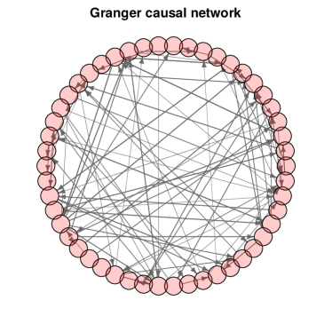
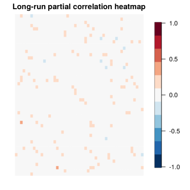
Figure 5: Estimated networks for data simulated as in Data generation. Left: Granger causal network $\mathcal{N}^{\text{{G}}}$. A directed arrow from node $i$ to node $i^{\prime}$ indicates that variable $i$ Granger causes node $i^{\prime}$, and the edge weights proportional to the size of estimated coefficients are visualised by the edge width. Right: Long-run partial correlation network $\mathcal{N}^{\text{{L}}}$ where the edge weights (i.e. partial correlations) are visualised by the colour.

Forecasting

The fnets objects are supported by the predict method with which we can forecast the input data n.ahead steps. For example, we can produce a one-step ahead forecast of $\mathbf{X}_{n+1}$ as

pr <- predict(out, n.ahead = 1, fc.restricted = TRUE)pr$forecastThe argument fc.restricted specifies whether to use the estimator $\widehat{\bm{\chi}}^{\text{{res}}}_{n+h|n}$ in (17) generated under a restricted factor model (3), or $\widehat{\bm{\chi}}^{\text{{unr}}}_{n+h|n}$ in (16) generated without such a restriction. Table 2 lists the entries from the output from predict.fnets. We can similarly produce forecasts from fnets objects output from fnets.var, or fm objects from fnets.factor.model.

Table 2: Entries of the output from predict.fnets

Name	Description	Type
forecast	$h\times p$ matrix containing the $h$-step ahead forecasts of $\mathbf{X}_{t}$	matrix
common.predict	A list containing	list
$is	$n\times p$ matrix containing the in-sample estimator of $\bm{\chi}_{t}$
$fc	$h\times p$ matrix containing the $h$-step ahead forecasts of $\bm{\chi}_{t}$
$h	Input parameter
$r	Factor number (only produced when fc.restricted = TRUE)
idio.predict	A list containing is, fc and h, see common.predict	list
mean.x	Sample mean vector	vector

Factor number estimation

It is of independent interest to estimate the number of factors (if any) in the input dataset. The function factor.number provides access to the two methods for selecting $q$ described in Factor numbers $q$ and $r$. The following code calls the information criterion-based factor number estimation method in (19), and prints the output:

fn <- factor.number(x, fm.restricted = FALSE)print(fn)Factor number selectionFactor model: unrestrictedMethod: Information criterionNumber of factors:IC1: 2IC2: 2IC3: 3IC4: 2IC5: 2IC6: 2Calling plot(fn) returns Figure 3 which visualises the factor number estimators from six information criteria implemented. Alternatively, we call the eigenvalue ratio-based method in (20) as

fn <- factor.number(x, method = "er", fm.restricted = FALSE)In this case, plot(fn) produces a plot of $\text{ER}(b)$ against the candidate factor number $b\in\{1,\ldots,\bar{q}\}$.

Visualisation of tuning parameter selection procedures

The method for threshold selection discussed in Threshold $\mathfrak{t}$ is implemented by the threshold function, which returns objects of threshold class supported by print and plot methods.

th <- threshold(out$idio.var$beta)thThresholded matrixThreshold: 0.0297308643Non-zero entries: 62/2500The call plot(th) generates Figure 4. Additionally, we provide tools for visualising the tuning parameter selection results adopted in Steps 2 and 3 of FNETS (see VAR order $d$, $\lambda$ and $\eta$). These tools are accessible from both fnets and fnets.var by calling the plot method with the argument display = "tuning", e.g.

set.seed(111)n <- 500p <- 10x <- sim.var(n, p)$dataout1 <- fnets(x, q = 0, var.order = 1:3, tuning.args = list(tuning = "cv"))plot(out1, display = "tuning")This generates the two plots reported in Figure 6 which visualise the CV errors computed as described in Cross validation and, in particular, the left plot shows that the VAR order is correctly selected by this approach. When tuning.args contains tuning = "bic", the results from the eBIC method described in Extended Bayesian information criterion adopted in Step 2, is similarly visualised in place of the left panel of Figure 6.

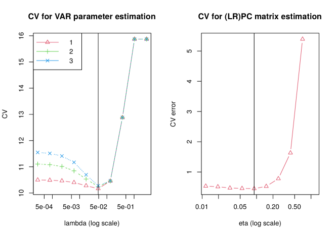
Figure 6: Plots of CV$(\lambda,b)$ against $\lambda$ with $b\in\{1,2,3\}$ (left) and CV$(\eta)$ against $\eta$ (right). Vertical lines denote where the minimum CV measure is attained with respect to $\lambda$ and $\eta$, respectively.

Simulations

Barigozzi et al. (2022) provide comprehensive simulation results on the estimation and forecasting performance of FNETS in comparison with competing methodologies. Therefore in this paper, we focus on assessing the performance of the methods for selecting tuning parameters such as the threshold and VAR order discussed in Tuning parameter selection. Additionally in Appendix B, we compare the adaptive and the non-adaptive estimators in estimating $\bm{\Delta}$ and also investigate how their performance is carried over to estimating $\bm{\Omega}$.

Settings

We consider the following data generating processes for the factor-driven component $\bm{\chi}_{t}$:

1. Taken from Forni et al. (2017), $\chi_{it}$ is generated as a sum of AR processes $\chi_{it}=\sum_{j=1}^{q}a_{ij}(1-\alpha_{ij}L)^{-1}u_{jt}$ with $q=2$, where $u_{jt}\sim_{\text{iid}}\mathcal{N}(0,1)$, $a_{ij}\sim_{\text{iid}}\mathcal{U}[-1,1]$ and $\alpha_{ij}\sim_{\text{iid}}\mathcal{U}[-0.8,0.8]$ with $\mathcal{U}[a,b]$ denoting a uniform distribution. Then, $\bm{\chi}_{t}$ does not admit a static representation in (3).

2. $\bm{\chi}_{t}=\mathbf{0}$, i.e. the VAR process is directly observed as $\mathbf{X}_{t}=\bm{\xi}_{t}$.

For generating a VAR($d$) process $\bm{\xi}_{t}$, we first generate a directed Erdős-Rényi random graph $\mathcal{N}=(\mathcal{V},\mathcal{E})$ on $\mathcal{V}=\{1,\ldots,p\}$ with the link probability $1/p$, and set entries of $\mathbf{A}_{d}$ such that $A_{d,ii^{\prime}}=0.275$ when $(i,i^{\prime})\in\mathcal{E}$ and $A_{d,ii^{\prime}}=0$ otherwise. Also, we set $\mathbf{A}_{\ell}=\mathbf{O}$ for $\ell<d$. The VAR innovations are generated as below.

1. Gaussian with the covariance matrix $\bm{\Gamma}=\bm{\Delta}^{-1}=\mathbf{I}$.

2. Gaussian with the covariance matrix $\bm{\Gamma}=\bm{\Delta}^{-1}$ such that $\delta_{ii}=1$, $\delta_{i,i+1}=\delta_{i+1,i}=0.6$, $\delta_{i,i+2}=\delta_{i+2,i}=0.3$, and $\delta_{ii^{\prime}}=0$ for $|i-i^{\prime}|\geq 3$.

For each setting, we generate $100$ realisations.

Results: Threshold selection

We assess the performance of the adaptive threshold. We generate $\bm{\chi}_{t}$ as in (C1) and fix $d=1$ for generating $\bm{\xi}_{t}$ and further, treat $d$ as known. We consider $(n,p)\in\{(200,50),(200,100),(500,100),(500,200)\}$. Then we estimate $\bm{\Omega}$ using the thresholded Lasso estimator of $\mathbf{A}_{1}$ (see (11) and (13)) with two choices of thresholds, $\mathfrak{t}=\mathfrak{t}_{\text{ada}}$ generated as described in Threshold $\mathfrak{t}$ and $\mathfrak{t}=0$. To assess the performance of $\widehat{\bm{\Omega}}=[\widehat{\omega}_{ii^{\prime}}]$ in recovering of the support of $\bm{\Omega}=[\omega_{ii^{\prime}}]$, i.e. $\{(i,i^{\prime}):\,\omega_{ii^{\prime}}\neq 0\}$, we plot the receiver operating characteristic (ROC) curves of true positive rate (TPR) against false positive rate (FPR), where

$$\text{TPR}=\frac{|\{(i,i^{\prime}):\,\widehat{\omega}_{ii^{\prime}}\neq 0\text{ and }\omega_{ii^{\prime}}\neq 0\}|}{|\{(i,i^{\prime}):\,\omega_{ii^{\prime}}\neq 0\}|}\quad\text{and}\quad\text{FPR}=\frac{|\{(i,i^{\prime}):\,\widehat{\omega}_{ii^{\prime}}\neq 0\text{ and }\omega_{ii^{\prime}}=0\}|}{|\{(i,i^{\prime}):\,\omega_{ii^{\prime}}=0\}|}.$$

Figure 7 plots the ROC curves averaged over $100$ realisations when $\mathfrak{t}=\mathfrak{t}_{\text{ada}}$ and $\mathfrak{t}=0$. When $\bm{\Delta}=\mathbf{I}$ under (E1), we see little improvement from adopting $\mathfrak{t}_{\text{ada}}$ as the support recovery performance is already good even without thresholding. However, when $\bm{\Delta}\neq\mathbf{I}$ under (E2), the adaptive threshold leads to improved support recovery especially when the sample size is large. Tables 3 and 4 in Appendix C additionally report the errors in estimating $\mathbf{A}_{1}$ and $\bm{\Omega}$ with and without thresholding, where we see little change is brought by thresholding. In summary, we conclude that the estimators already perform reasonably well without thresholding, and the adaptive threshold $\mathfrak{t}_{\text{ada}}$ brings marginal improvement in support recovery which is of interest in network estimation.

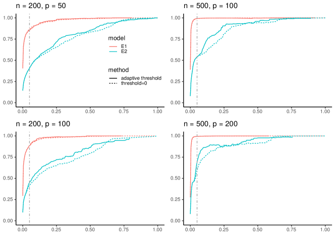
Figure 7: ROC curves of TPR against FPR for $\widetilde{\bm{\beta}}(\mathfrak{t})$ (13) (with $\widehat{\bm{\beta}}=\widehat{\bm{\beta}}^{\text{{las}}}$) when $\mathfrak{t}=\mathfrak{t}_{ada}$ and $\mathfrak{t}=0$ in recovering the support of $\bm{\Omega}$, averaged over $100$ realisations. Vertical lines indicate FPR $=0.05$

Results: VAR order selection

We compare the performance of the CV and eBIC methods proposed in VAR order $d,\lambda$ and $\eta$ for selecting the order of the VAR process. Here, we consider the case when $\bm{\chi}_{t}=\mathbf{0}$ (setting (C2)) and when $\bm{\xi}_{t}$ is generated under (E1) with $d\in\{1,3\}$. We set $(n,p)\in\{(200,10),(200,20),(500,10),(500,20)\}$ where the range of $p$ is in line with the simulation studies conducted in the relevant literature (see e.g. Zheng (2022)). We consider $\{1,2,3,4\}$ as the candidate VAR orders. Figure 8 and Table 5 in Appendix C show that CV works reasonably well regardless of $d\in\{1,3\}$, with slightly better performance observed together with the DS estimator. On the other hand, eBIC tends to over-estimate the VAR order when $d=1$ while under-estimating it when $d=3$, and hence is less reliable compared to the CV method.

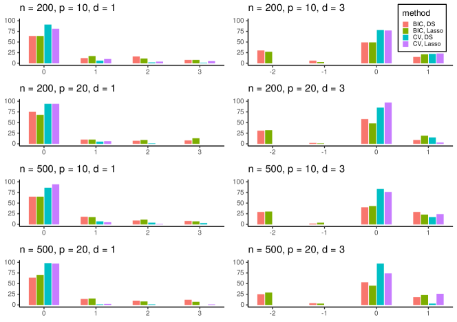
Figure 8: Box plots of $\widehat{d}-d$ over $100$ realisations when the VAR order is selected by the CV and eBIC methods in combination with the Lasso (11) and the DS (12) estimators.

Data example

Energy price data

Electricity is more difficult to store than physical commodities which results in high volatility and seasonality in spot prices (Han et al., 2022). Global market deregulation has increased the volume of electricity trading, which promotes the development of better forecasting and risk management methods. We analyse a dataset of node-specific prices in the PJM (Pennsylvania, New Jersey and Maryland) power pool area in the United States, accessed using dataminer2.pjm.com. There are four node types in the panel, which are Zone, Aggregate, Hub and Extra High Voltage (EHV); for their definitions, see Table 8 and for the names and types of $p=50$ nodes, see Table 9, all found in Appendix D. The series we model is the sum of the real time congestion price and marginal loss price or, equivalently, the difference between the spot price at a given location and the overall system price, where the latter can be thought of as an observed factor in the local spot price. These are obtained as hourly prices and then averaged over each day as per Maciejowska and Weron (2013). We remove any short-term seasonality by subtracting a separate mean for each day of the week. Since the energy prices may take negative values, we adopt the inverse hyperbolic sine transformation as in Uniejewski et al. (2017) for variance stabilisation.

Network estimation

We analyse the data collected between 01/01/2021 and 19/07/2021 ($n=200$). The information criterion in (19) returns a single factor ($\widehat{q}=1$), and $\widehat{d}=1$ is selected by CV. See Figure 9 for the heat maps visualising the three networks $\mathcal{N}^{\text{{G}}}$, $\mathcal{N}^{\text{{C}}}$ and $\mathcal{N}^{\text{{L}}}$ described in Networks, which are produced by fnets.

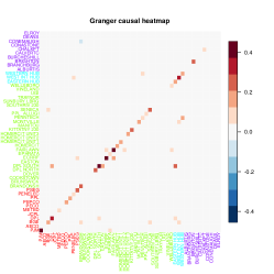
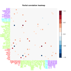
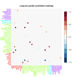
Figure 9: Heat maps of the three networks underlying the energy price data collected over the period 01/01/2021–19/07/2021. Left: $\mathcal{N}^{\text{{G}}}$ obtained with the Lasso estimator (11) combined with the adaptive threshold $\mathfrak{t}_{\text{ada}}$. Middle: $\mathcal{N}^{\text{{C}}}$ obtained with the ACLIME estimator of $\bm{\Delta}$. Right: $\mathcal{N}^{\text{{L}}}$ obtained by combining the estimators of VAR parameters and $\bm{\Delta}$. In the axis labels, Zone-type nodes are coloured in red, Aggregate-types in green, Hub-types in blue and EHV-types in purple.

The non-zero entries of the VAR parameter matrix estimates tend to take positive values, indicating that high energy prices are persistent and spill over to other nodes. Considering the node types, Hub-type nodes (blue) tend to have out-going edges to nodes of different types, which reflects the behaviour of the electrical transmission system. Some Zone-type nodes (red) have several in-coming edges from Aggregate-types (green) and Hub-types, while EHV-types (purple) have few edges in $\mathcal{N}^{\text{{G}}}$, which carries forward to $\mathcal{N}^{\text{{L}}}$ where we observe that those Zone-type nodes have strong long-run correlations with other nodes while EHV-types do not.

Summary

We introduce the R package fnets which implements the FNETS methodology proposed by Barigozzi et al. (2022) for network estimation and forecasting of high-dimensional time series exhibiting strong correlations. It further implements data-driven methods for selecting tuning parameters, and provides tools for high-dimensional time series factor modelling under the GDFM which are of independent interest. The efficacy of our package is demonstrated on both real and simulated datasets.

Dom Owens
School of Mathematics, University of Bristol
Supported by EPSRC Centre for Doctoral Training (EP/S023569/1)
dom.owens@bristol.ac.uk

Haeran Cho
School of Mathematics, University of Bristol
Supported by the Leverhulme Trust (RPG-2019-390)
haeran.cho@bristol.ac.uk

Matteo Barigozzi
Department of Economics, Università di Bologna
Supported by MIUR (PRIN 2017, Grant 2017TA7TYC)
matteo.barigozzi@unibo.it

Appendix A: Information criteria for factor number selection

Here we list information criteria for factor number estimation which are implemented in fnets and accessible by the functions fnets, fnets.factor.model and factor.number by setting the argument ic.op at an integer belonging to $\{1,\ldots,6\}$. When fm.restricted = FALSE, we have

• $\left(\frac{1}{p}\sum_{j=b+1}^{p}\frac{1}{2m+1}\sum_{k=-m}^{m}\widehat{\mu}_{x,j}(\omega_{k})\right)+b\cdot c\cdot(m^{-2}+\sqrt{m/n}+p^{-1})\cdot\log(\min(p,m^{2},\sqrt{n/m}))$,

• $\left(\frac{1}{p}\sum_{j=b+1}^{p}\frac{1}{2m+1}\sum_{k=-m}^{m}\widehat{\mu}_{x,j}(\omega_{k})\right)+b\cdot c\cdot(\min(p,m^{2},\sqrt{n/m}))^{-1/2}$,

• $\left(\frac{1}{p}\sum_{j=b+1}^{p}\frac{1}{2m+1}\sum_{k=-m}^{m}\widehat{\mu}_{x,j}(\omega_{k})\right)+b\cdot c\cdot(\min(p,m^{2},\sqrt{n/m}))^{-1}\cdot\log(\min(p,m^{2},\sqrt{n/m}))$,

• $\log\left(\frac{1}{p}\sum_{j=b+1}^{p}\frac{1}{2m+1}\sum_{k=-m}^{m}\widehat{\mu}_{x,j}(\omega_{k})\right)+b\cdot c\cdot(m^{-2}+\sqrt{m/n}+p^{-1})\cdot\log(\min(p,m^{2},\sqrt{n/m}))$,

• $\log\left(\frac{1}{p}\sum_{j=b+1}^{p}\frac{1}{2m+1}\sum_{k=-m}^{m}\widehat{\mu}_{x,j}(\omega_{k})\right)+b\cdot c\cdot(\min(p,m^{2},\sqrt{n/m}))^{-1/2}$,

• $\log\left(\frac{1}{p}\sum_{j=b+1}^{p}\frac{1}{2m+1}\sum_{k=-m}^{m}\widehat{\mu}_{x,j}(\omega_{k})\right)+b\cdot c\cdot(\min(p,m^{2},\sqrt{n/m}))^{-1}\cdot\log(\min(p,m^{2},\sqrt{n/m}))$ .

When fm.restricted = TRUE, we use one of

• $\left(\frac{1}{p}\sum_{j=b+1}^{p}\widehat{\mu}_{x,j}\right)+b\cdot c\cdot(n+p)/(np)\cdot\log(np/(n+p))$,

• $\left(\frac{1}{p}\sum_{j=b+1}^{p}\widehat{\mu}_{x,j}\right)+b\cdot c\cdot(n+p)/(np)\cdot\log(np/(n+p))$,

• $\left(\frac{1}{p}\sum_{j=b+1}^{p}\widehat{\mu}_{x,j}\right)+b\cdot c\cdot\log(\min(n,p))/(\min(n,p))$,

• $\log\left(\frac{1}{p}\sum_{j=b+1}^{p}\widehat{\mu}_{x,j}\right)+b\cdot c\cdot(n+p)/(np)\cdot\log(np/(n+p))$,

• $\log\left(\frac{1}{p}\sum_{j=b+1}^{p}\widehat{\mu}_{x,j}\right)+b\cdot c\cdot(n+p)/(np)\cdot\log(np/(n+p))$,

• $\log\left(\frac{1}{p}\sum_{j=b+1}^{p}\widehat{\mu}_{x,j}\right)+b\cdot c\cdot\log(\min(n,p))/(\min(n,p))$.

Whether fm.restricted = FALSE or not, the default choice is ic.op = 5.

Appendix B: ACLIME estimator

We provide a detailed description of the adaptive extension of the CLIME estimator of $\bm{\Delta}$ in (14), extending the methodology proposed in Cai et al. (2016) for precision matrix estimation in the independent setting. Let $\widehat{\bm{\Gamma}}^{*}=\widehat{\bm{\Gamma}}+n^{-1}{\mathbf{I}}$ and $\eta_{1}=2\sqrt{{\log(p)}/{n}}$ .

1. Let $\check{\bm{\Delta}}^{(1)}=[\check{\delta}_{ii^{\prime}}^{(1)}]$ be the solution to

   $$\check{\bm{\Delta}}^{(1)}_{\cdot i^{\prime}}={\arg\min}_{\mathbf{m}\in R^{p}}|\mathbf{m}|_{1}\quad\text{subject to}$$ (22)

   $$\left|(\widehat{\bm{\Gamma}}^{*}\mathbf{m}-\mathbf{e}_{i^{\prime}})_{i}\right|\leq\eta_{1}(\widehat{\gamma}_{ii}\vee\widehat{\gamma}_{i^{\prime}i^{\prime}})m_{i^{\prime}}\ \forall\ 1\leq i\leq p\text{ \ and \ }m_{i^{\prime}}>0,$$

   for $i^{\prime}=1,\ldots,p$. Then we obtain truncated estimates

   $$\widehat{\delta}_{ii}^{(1)}=\check{\delta}_{ii}^{(1)}\cdot\mathbb{I}_{\{|\widehat{\gamma}_{ii}|\leq\sqrt{n/\log(p)}\}}+\sqrt{\frac{\log(p)}{n}}\cdot\mathbb{I}_{\{|\widehat{\gamma}_{ii}|>\sqrt{n/\log(p)}\}}.$$

2. We obtain

   $$\check{\bm{\Delta}}^{(2)}_{\cdot i^{\prime}} ={\arg\min}_{\mathbf{m}\in\mathbb{R}^{p}}|\mathbf{m}|_{1}\quad\text{subject to}\quad\left|(\widehat{\bm{\Gamma}}^{*}\mathbf{m}-\mathbf{e}_{i^{\prime}})_{i}\right|\leq\eta_{2}\sqrt{\widehat{\gamma}_{ii}\widehat{\delta}_{i^{\prime}i^{\prime}}^{(1)}}\quad\forall\ 1\leq i\leq p,$$

   where $\eta_{2}>0$ is a tuning parameter. Since $\check{\bm{\Delta}}^{(2)}$ is not guaranteed to be symmetric, the final estimator is obtained after a symmetrisation step:

   $$\widehat{\bm{\Delta}}_{ada} =[\widehat{\delta}_{ii^{\prime}},\,1\leq i,i^{\prime}\leq p]\text{ with }\widehat{\delta}_{ii^{\prime}}^{(2)}=\check{\delta}_{ii^{\prime}}^{(2)}\cdot\mathbb{I}_{\{|\check{\delta}_{ii^{\prime}}^{(2)}|\leq|\check{\delta}_{i^{\prime}i}^{(2)}|\}}+\check{\delta}_{i^{\prime}i}^{(2)}\cdot\mathbb{I}_{\{|\check{\delta}_{i^{\prime}i}^{(2)}|<|\check{\delta}_{ii^{\prime}}^{(2)}|\}}.$$ (23)

The constraints in (22) incorporate the parameter in the right-hand side. To use linear programming software to solve this, we formulate the constraints for each $1\leq i^{\prime}\leq p$ as

$$\forall 1\leq i\leq p,\quad((\widehat{\bm{\Gamma}}^{*}-\bm{Q}^{i^{\prime}})\mathbf{m}-\mathbf{e}_{i^{\prime}})_{i}\leq 0,$$

$$\forall 1\leq i\leq p,\quad-((\widehat{\bm{\Gamma}}^{*}+\bm{Q}^{i^{\prime}})\mathbf{m}-\mathbf{e}_{i^{\prime}})_{i}\leq 0,$$

$$m_{i^{\prime}}>0.$$

where $\bm{Q}^{i^{\prime}}$ has entries $q_{ii^{\prime}}=\eta_{1}(\widehat{\gamma}_{ii}\vee\widehat{\gamma}_{i^{\prime}i^{\prime}})$ in column $i^{\prime}$ and $0$ elsewhere.

Appendix C: Additional simulation results

Threshold selection

Tables 3 and 4 report the errors in estimating $\mathbf{A}_{1}$ and $\bm{\Omega}$ when the threshold $\mathfrak{t}=\mathfrak{t}_{\text{ada}}$ or $\mathfrak{t}=0$ is applied to the estimator of $\mathbf{A}_{1}$ obtained by either the Lasso (11) or the DS (12) estimators. With a matrix $\bm{\gamma}$ as an estimand we measure the estimation error of its estimator $\widehat{\bm{\gamma}}$ using the following (scaled) matrix norms:

$$L_{F}=\frac{\|\widehat{\bm{\gamma}}-\bm{\gamma}\|_{F}}{\|\bm{\gamma}\|_{F}}\quad\text{and}\quad L_{2}=\frac{\|\widehat{\bm{\gamma}}-\bm{\gamma}\|}{\|\bm{\gamma}\|}.$$

Table 3: Errors in estimating $\mathbf{A}_{1}$ with $\mathfrak{t}\in\{0,\mathfrak{t}_{\text{ada}}\}$ in combination with the Lasso (11) and the DS (12) estimators, measured by $L_{F}$ and $L_{2}$, averaged over $100$ realisations (with standard errors reported in brackets). We also report the average TPR when FPR $=0.05$ and the corresponding standard error. See Results: Threshold selection in the main text for further information.

			$\mathfrak{t}=0$						$\mathfrak{t}=\mathfrak{t}_{\text{ada}}$
			$\widehat{\bm{\beta}}^{\text{{las}}}$			$\widehat{\bm{\beta}}^{\text{{DS}}}$			$\widehat{\bm{\beta}}^{\text{{las}}}$			$\widehat{\bm{\beta}}^{\text{{DS}}}$
Model	n	p	TPR	$L_{F}$	$L_{2}$	TPR	$L_{F}$	$L_{2}$	TPR	$L_{F}$	$L_{2}$	TPR	$L_{F}$	$L_{2}$
(E1)	200	50	0.9681	0.6234	0.7204	0.8991	0.4299	0.3747	0.9413	0.6226	0.7204	0.6932	0.4487	0.3960
			(0.050)	(0.081)	(0.118)	(0.096)	(0.280)	(0.225)	(0.112)	(0.088)	(0.121)	(0.216)	(0.256)	(0.206)
	200	100	0.9398	0.6696	0.8113	0.8810	0.5772	0.4362	0.8832	0.6710	0.8132	0.6491	0.6025	0.4642
			(0.091)	(0.096)	(0.096)	(0.094)	(0.449)	(0.271)	(0.182)	(0.108)	(0.100)	(0.246)	(0.418)	(0.250)
	500	100	0.9990	0.4648	0.6682	0.9304	0.2740	0.2604	0.9971	0.4608	0.6645	0.7237	0.2806	0.2699
			(0.003)	(0.054)	(0.094)	(0.065)	(0.158)	(0.138)	(0.010)	(0.056)	(0.095)	(0.199)	(0.133)	(0.111)
	500	200	0.9986	0.5068	0.7729	0.9167	0.3680	0.3882	0.9964	0.5023	0.7637	0.7095	0.3889	0.4014
			(0.003)	(0.058)	(0.081)	(0.076)	(0.196)	(0.134)	(0.006)	(0.061)	(0.082)	(0.256)	(0.187)	(0.126)
(E2)	200	50	0.9595	0.6375	0.7075	0.8828	0.4673	0.4280	0.9442	0.6356	0.7079	0.6720	0.4835	0.4433
			(0.053)	(0.077)	(0.094)	(0.107)	(0.324)	(0.255)	(0.064)	(0.079)	(0.096)	(0.212)	(0.303)	(0.241)
	200	100	0.9624	0.6200	0.6909	0.8093	0.4519	0.4090	0.9435	0.6175	0.6913	0.5903	0.4765	0.4324
			(0.072)	(0.079)	(0.089)	(0.100)	(0.385)	(0.251)	(0.093)	(0.082)	(0.090)	(0.182)	(0.371)	(0.243)
	500	100	0.9970	0.4657	0.5533	0.9304	0.3434	0.3621	0.9958	0.4638	0.5525	0.8384	0.3370	0.3634
			(0.006)	(0.056)	(0.076)	(0.089)	(0.158)	(0.153)	(0.008)	(0.058)	(0.077)	(0.182)	(0.140)	(0.144)
	500	200	0.9981	0.4702	0.5658	0.9205	0.3684	0.3740	0.9945	0.4686	0.5665	0.8154	0.3663	0.3803
			(0.003)	(0.065)	(0.091)	(0.088)	(0.182)	(0.162)	(0.014)	(0.068)	(0.093)	(0.205)	(0.159)	(0.145)

Table 4: Errors in estimating $\bm{\Omega}$ with $\mathfrak{t}\in\{0,\mathfrak{t}_{\text{ada}}\}$ applied to the estimator of $\mathbf{A}_{1}$ in combination with the Lasso (11) and the DS (12) estimators, measured by $L_{F}$ and $L_{2}$, averaged over $100$ realisations (with standard errors reported in brackets). We also report the average TPR when FPR $=0.05$ and the corresponding standard error. See Results: Threshold selection in the main text for further information.

			$\mathfrak{t}=0$						$\mathfrak{t}=\mathfrak{t}_{\text{ada}}$
			$\widehat{\bm{\beta}}^{\text{{las}}}$			$\widehat{\bm{\beta}}^{\text{{DS}}}$			$\widehat{\bm{\beta}}^{\text{{las}}}$			$\widehat{\bm{\beta}}^{\text{{DS}}}$
Model	n	p	TPR	$L_{F}$	$L_{2}$	TPR	$L_{F}$	$L_{2}$	TPR	$L_{F}$	$L_{2}$	TPR	$L_{F}$	$L_{2}$
(E1)	200	50	0.8714	0.4143	0.5553	0.8622	0.4217	0.5691	0.8685	0.4145	0.5559	0.8640	0.4217	0.5695
			(0.108)	(0.048)	(0.066)	(0.119)	(0.054)	(0.070)	(0.118)	(0.049)	(0.067)	(0.121)	(0.055)	(0.070)
	200	100	0.8827	0.4320	0.5890	0.8961	0.4379	0.5949	0.8684	0.4326	0.5892	0.8867	0.4386	0.5960
			(0.084)	(0.050)	(0.072)	(0.080)	(0.046)	(0.065)	(0.139)	(0.052)	(0.074)	(0.120)	(0.048)	(0.066)
	500	100	0.9909	0.3311	0.4916	0.9886	0.3391	0.4989	0.9928	0.3303	0.4901	0.9901	0.3380	0.4975
			(0.016)	(0.031)	(0.069)	(0.021)	(0.036)	(0.065)	(0.015)	(0.032)	(0.069)	(0.018)	(0.037)	(0.066)
	500	200	0.9942	0.3520	0.5287	0.9916	0.3511	0.5400	0.9954	0.3512	0.5273	0.9672	0.3528	0.5399
			(0.009)	(0.038)	(0.054)	(0.018)	(0.045)	(0.065)	(0.008)	(0.039)	(0.055)	(0.129)	(0.055)	(0.072)
(E2)	200	50	0.4074	0.7831	0.8353	0.4027	0.7942	0.8335	0.4063	0.7832	0.8353	0.4045	0.7943	0.8336
			(0.073)	(0.089)	(0.072)	(0.087)	(0.079)	(0.034)	(0.072)	(0.089)	(0.072)	(0.089)	(0.079)	(0.034)
	200	100	0.4178	0.8406	0.8690	0.3541	0.9119	0.8879	0.4486	0.8407	0.8690	0.4038	0.9120	0.8880
			(0.091)	(0.108)	(0.036)	(0.107)	(0.126)	(0.045)	(0.091)	(0.108)	(0.036)	(0.123)	(0.126)	(0.045)
	500	100	0.5405	0.8267	0.8118	0.5632	0.7910	0.7953	0.5406	0.8267	0.8117	0.5628	0.7910	0.7951
			(0.111)	(0.125)	(0.047)	(0.122)	(0.166)	(0.062)	(0.111)	(0.125)	(0.047)	(0.123)	(0.166)	(0.062)
	500	200	0.5951	0.8713	0.8519	0.6487	0.8184	0.8259	0.6918	0.8713	0.8519	0.7101	0.8184	0.8258
			(0.175)	(0.165)	(0.088)	(0.159)	(0.182)	(0.090)	(0.148)	(0.165)	(0.088)	(0.122)	(0.182)	(0.090)

VAR order selection

Table 5 reports the results of VAR order estimation over $100$ realisations.

Table 5: Distribution of $\widehat{d}-d$ over $100$ realisations when the VAR order is selected by the CV and eBIC methods in combination with the Lasso (11) and the DS (12) estimators, see Results: VAR order selection in the main text for further information.

			CV								eBIC
			$\widehat{\bm{\beta}}^{\text{{las}}}$				$\widehat{\bm{\beta}}^{\text{{DS}}}$				$\widehat{\bm{\beta}}^{\text{{las}}}$				$\widehat{\bm{\beta}}^{\text{{DS}}}$
$d$	$n$	$p$	0	1	2	3	0	1	2	3	0	1	2	3	0	1	2	3
1	200	10	81	10	4	5	91	6	2	1	64	17	11	8	64	12	16	8
	200	20	94	6	0	0	94	5	1	0	68	10	9	13	75	10	7	8
	500	10	94	5	1	0	86	7	4	3	65	17	11	7	65	18	9	8
	500	20	97	2	0	1	98	1	1	0	70	15	8	7	64	14	10	12
			-2	-1	0	1	-2	-1	0	1	-2	-1	0	1	-2	-1	0	1
3	200	10	0	0	77	23	0	0	78	22	27	3	49	21	30	6	49	15
	200	20	0	0	97	3	0	0	85	15	32	1	48	19	31	2	58	9
	500	10	0	0	76	24	0	0	83	17	30	4	43	23	29	2	40	29
	500	20	0	0	74	26	0	0	97	3	29	3	45	23	25	4	53	18

CLIME vs. ACLIME estimators

We compare the performance of the adaptive and non-adaptive estimators for the VAR innovation precision matrix $\bm{\Delta}$ and its impact on the estimation of $\bm{\Omega}$, the inverse of the long-run covariance matrix of the data (see Step 3). We generate $\bm{\chi}_{t}$ as in (C1), fix $d=1$ and treat it as known and consider $(n,p)\in\{(200,50),(200,100),(500,100),(500,200)\}$.

In Tables 6 and 7, we report the errors of $\bm{\Delta}$ and $\bm{\Omega}$. We consider both the Lasso (11) and DS (12) estimators of VAR parameters, and CLIME and ACLIME estimators for $\bm{\Delta}$, which lead to four different estimators for $\bm{\Delta}$ and $\bm{\Omega}$, respectively. Overall, we observe that with increasing $n$, the performance of all estimators improve according to all metrics regardless of the scenarios (E1) or (E2), while increasing $p$ has an adverse effect. The two methods perform similarly in setting (E1) when $\bm{\Delta}=\mathbf{I}$. There is marginal improvement for adopting the ACLIME estimator noticeable under (E2), particularly in TPR. Figures 10 and 11 shows the ROC curves for the support recovery of $\bm{\Delta}$ and $\bm{\Omega}$ when the Lasso estimator is used.

Table 6: Errors in estimating $\bm{\Delta}$ using CLIME and ACLIME estimators, measured by $L_{F}$ and $L_{2}$, averaged over $100$ realisations (with standard errors reported in brackets). We also report the average TPR when FPR $=0.05$ and the corresponding standard errors.

			CLIME						ACLIME
			$\widehat{\bm{\beta}}^{\text{{las}}}$			$\widehat{\bm{\beta}}^{\text{{DS}}}$			$\widehat{\bm{\beta}}^{\text{{las}}}$			$\widehat{\bm{\beta}}^{\text{{DS}}}$
Model	n	p	TPR	$L_{F}$	$L_{2}$	TPR	$L_{F}$	$L_{2}$	TPR	$L_{F}$	$L_{2}$	TPR	$L_{F}$	$L_{2}$
(E1)	200	50	1.000	0.215	0.489	1.000	0.220	0.497	1.000	0.207	0.472	1.000	0.209	0.469
			(0.000)	(0.047)	(0.223)	(0.000)	(0.047)	(0.182)	(0.002)	(0.043)	(0.173)	(0.000)	(0.041)	(0.116)
	200	100	1.000	0.235	0.513	1.000	0.241	0.521	1.000	0.223	0.507	1.000	0.228	0.518
			(0.000)	(0.036)	(0.089)	(0.000)	(0.036)	(0.107)	(0.000)	(0.033)	(0.084)	(0.000)	(0.034)	(0.099)
	500	100	1.000	0.181	0.458	1.000	0.183	0.466	1.000	0.176	0.452	1.000	0.178	0.458
			(0.000)	(0.022)	(0.062)	(0.000)	(0.029)	(0.087)	(0.000)	(0.022)	(0.052)	(0.000)	(0.028)	(0.069)
	500	200	1.000	0.198	0.510	1.000	0.193	0.492	1.000	0.187	0.505	1.000	0.182	0.489
			(0.000)	(0.027)	(0.066)	(0.000)	(0.035)	(0.065)	(0.000)	(0.026)	(0.056)	(0.000)	(0.033)	(0.057)
(E2)	200	50	0.659	0.422	0.816	0.662	0.391	0.608	0.682	0.397	0.706	0.687	0.380	0.600
			(0.058)	(0.101)	(0.654)	(0.057)	(0.031)	(0.144)	(0.055)	(0.056)	(0.351)	(0.054)	(0.030)	(0.176)
	200	100	0.639	0.417	0.695	0.637	0.420	0.720	0.669	0.404	0.663	0.668	0.405	0.684
			(0.044)	(0.039)	(0.205)	(0.042)	(0.043)	(0.249)	(0.041)	(0.037)	(0.162)	(0.039)	(0.037)	(0.193)
	500	100	0.730	0.372	0.764	0.726	0.499	1.708	0.735	0.358	0.650	0.734	0.361	0.718
			(0.035)	(0.097)	(0.828)	(0.039)	(1.101)	(7.586)	(0.032)	(0.038)	(0.322)	(0.031)	(0.056)	(0.517)
	500	200	0.729	0.370	0.711	0.728	0.362	0.736	0.737	0.363	0.647	0.737	0.354	0.673
			(0.028)	(0.035)	(0.355)	(0.028)	(0.035)	(0.384)	(0.023)	(0.026)	(0.239)	(0.024)	(0.028)	(0.279)

Table 7: Errors in estimating $\bm{\Omega}$ using CLIME and ACLIME estimators of $\bm{\Delta}$, measured by $L_{F}$ and $L_{2}$, averaged over $100$ realisations (with standard errors reported in brackets). We also report the average TPR when FPR $=0.05$ and the corresponding standard errors.

			CLIME						ACLIME
			$\widehat{\bm{\beta}}^{\text{{las}}}$			$\widehat{\bm{\beta}}^{\text{{DS}}}$			$\widehat{\bm{\beta}}^{\text{{las}}}$			$\widehat{\bm{\beta}}^{\text{{DS}}}$
Model	n	p	TPR	$L_{F}$	$L_{2}$	TPR	$L_{F}$	$L_{2}$	TPR	$L_{F}$	$L_{2}$	TPR	$L_{F}$	$L_{2}$
(E1)	200	50	0.871	0.415	0.557	0.862	0.422	0.571	0.867	0.411	0.558	0.856	0.417	0.570
			(0.108)	(0.050)	(0.070)	(0.119)	(0.055)	(0.080)	(0.106)	(0.051)	(0.088)	(0.114)	(0.053)	(0.083)
	200	100	0.883	0.432	0.589	0.896	0.438	0.595	0.868	0.423	0.583	0.883	0.429	0.587
			(0.084)	(0.050)	(0.072)	(0.080)	(0.046)	(0.065)	(0.088)	(0.048)	(0.077)	(0.085)	(0.045)	(0.061)
	500	100	0.991	0.331	0.492	0.989	0.339	0.499	0.991	0.328	0.490	0.989	0.337	0.498
			(0.016)	(0.031)	(0.069)	(0.021)	(0.036)	(0.065)	(0.015)	(0.033)	(0.070)	(0.019)	(0.036)	(0.067)
	500	200	0.994	0.352	0.529	0.992	0.351	0.540	0.994	0.344	0.525	0.990	0.342	0.537
			(0.009)	(0.038)	(0.054)	(0.018)	(0.045)	(0.065)	(0.009)	(0.038)	(0.056)	(0.014)	(0.044)	(0.068)
(E2)	200	50	0.509	0.532	0.724	0.510	0.514	0.664	0.504	0.518	0.679	0.507	0.506	0.658
			(0.078)	(0.071)	(0.243)	(0.068)	(0.043)	(0.137)	(0.071)	(0.055)	(0.162)	(0.063)	(0.043)	(0.141)
	200	100	0.511	0.541	0.683	0.513	0.542	0.695	0.509	0.531	0.674	0.504	0.531	0.679
			(0.059)	(0.047)	(0.082)	(0.065)	(0.051)	(0.093)	(0.062)	(0.045)	(0.084)	(0.061)	(0.046)	(0.084)
	500	100	0.640	0.450	0.655	0.624	0.544	1.099	0.642	0.441	0.597	0.637	0.440	0.617
			(0.066)	(0.072)	(0.402)	(0.079)	(0.866)	(3.714)	(0.059)	(0.036)	(0.118)	(0.060)	(0.047)	(0.204)
	500	200	0.670	0.461	0.630	0.658	0.450	0.630	0.677	0.456	0.612	0.661	0.445	0.605
			(0.045)	(0.041)	(0.116)	(0.043)	(0.040)	(0.117)	(0.041)	(0.036)	(0.075)	(0.037)	(0.037)	(0.082)

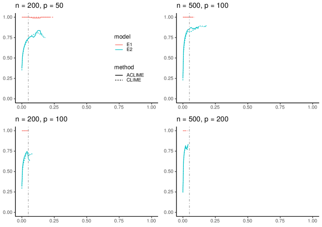
Figure 10: ROC curves of TPR against FPR for $\widehat{\bm{\Delta}}$ with CLIME and ACLIME estimators in recovering the support of $\bm{\Delta}$, averaged over $100$ realisations. Vertical lines indicate FPR $=0.05$.

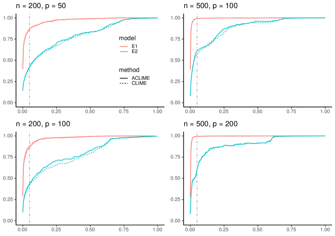
Figure 11: ROC curves of TPR against FPR for $\widehat{\bm{\Omega}}$ with CLIME and ACLIME estimators in recovering the support of $\bm{\Omega}$, averaged over $100$ realisations. Vertical lines indicate FPR $=0.05$.

Appendix D: Dataset information

Table 8 defines the four node types in the panel. Table 9 describes the dataset analysed in Data example.

Table 8: Node type definitions for energy price data.

Name	Definition
Zone	A transmission owner’s area within the PJM Region.
Aggregate	A group of more than one individual bus into a pricing node (pnode)
	that is considered as a whole in the Energy Market and other various systems
	and Markets within PJM.
Hub	A group of more than one individual bus into a regional pricing node (pnode)
	developed to produce a stable price signal in the Energy Market
	and other various systems and Markets within PJM.
Extra High Voltage (EHV)	Nodes at 345kV and above on the PJM system.

Table 9: Names, IDs and Types for the $50$ power nodes in the energy price dataset.

Name	Node ID	Node Type
PJM	1	ZONE
AECO	51291	ZONE
BGE	51292	ZONE
DPL	51293	ZONE
JCPL	51295	ZONE
METED	51296	ZONE
PECO	51297	ZONE
PEPCO	51298	ZONE
PPL	51299	ZONE
PENELEC	51300	ZONE
PSEG	51301	ZONE
BRANDONSH	51205	AGGREGATE
BRUNSWICK	51206	AGGREGATE
COOKSTOWN	51211	AGGREGATE
DOVER	51214	AGGREGATE
DPL NORTH	51215	AGGREGATE
DPL SOUTH	51216	AGGREGATE
EASTON	51218	AGGREGATE
ECRRF	51219	AGGREGATE
EPHRATA	51220	AGGREGATE
FAIRLAWN	51221	AGGREGATE
HOMERCIT	51229	AGGREGATE
HOMERCIT UNIT1	51230	AGGREGATE
HOMERCIT UNIT2	51231	AGGREGATE
HOMERCIT UNIT3	51232	AGGREGATE
KITTATNY 230	51238	AGGREGATE
MANITOU	51239	AGGREGATE
MONTVILLE	51241	AGGREGATE
PENNTECH	51246	AGGREGATE
PPL_ALLUGI	51252	AGGREGATE
SENECA	51255	AGGREGATE
SOUTHRIV 230	51261	AGGREGATE
SUNBURY LBRG	51270	AGGREGATE
TRAYNOR	51277	AGGREGATE
UGI	51279	AGGREGATE
VINELAND	51280	AGGREGATE
WELLSBORO	51285	AGGREGATE
EASTERN HUB	51217	HUB
WEST INT HUB	51287	HUB
WESTERN HUB	51288	HUB
ALBURTIS	52443	EHV
BRANCHBURG	52444	EHV
BRIGHTON	52445	EHV
BURCHESHILL	52446	EHV
CALVERTC	52447	EHV
CHALKPT	52448	EHV
CONASTONE	52449	EHV
CONEMAUGH	52450	EHV
DEANS	52451	EHV
ELROY	52452	EHV

References

- Ahn and Horenstein (2013) S. C. Ahn and A. R. Horenstein. Eigenvalue ratio test for the number of factors. Econometrica, 81(3):1203–1227, 2013.
- Alessi et al. (2010) L. Alessi, M. Barigozzi, and M. Capasso. Improved penalization for determining the number of factors in approximate factor models. Statistics & Probability Letters, 80(23-24):1806–1813, 2010.
- Avarucci et al. (2022) M. Avarucci, M. Cavicchioli, M. Forni, and P. Zaffaroni. The main business cycle shock(s): Frequency-band estimation of the number of dynamic factors. CEPR Discussion Paper No. DP17281, 2022.
- Bai (2003) J. Bai. Inferential theory for factor models of large dimensions. Econometrica, 71(1):135–171, 2003.
- Bai and Ng (2002) J. Bai and S. Ng. Determining the number of factors in approximate factor models. Econometrica, 70:191–221, 2002.
- Bai (2021) P. Bai. LSVAR: Estimation of Low Rank Plus Sparse Structured Vector Auto-Regressive (VAR) Model, 2021. URL https://CRAN.R-project.org/package=LSVAR. R package version 1.2.
- Barigozzi and Brownlees (2019) M. Barigozzi and C. Brownlees. Nets: Network estimation for time series. Journal of Applied Econometrics, 34:347–364, 2019.
- Barigozzi et al. (2022) M. Barigozzi, H. Cho, and D. Owens. Fnets: Factor-adjusted network estimation and forecasting for high-dimensional time series. arXiv preprint arXiv:2201.06110, 2022.
- Basu and Michailidis (2015) S. Basu and G. Michailidis. Regularized estimation in sparse high-dimensional time series models. The Annals of Statistics, 43:1535–1567, 2015.
- Beck and Teboulle (2009) A. Beck and M. Teboulle. A fast iterative shrinkage-thresholding algorithm for linear inverse problems. SIAM Journal on Imaging Sciences, 2(1):183–202, 2009.
- Bergmeir et al. (2018) C. Bergmeir, R. J. Hyndman, and B. Koo. A note on the validity of cross-validation for evaluating autoregressive time series prediction. Computational Statistics & Data Analysis, 120:70–83, 2018.
- Bernanke et al. (2005) B. S. Bernanke, J. Boivin, and P. Eliasz. Measuring the effects of monetary policy: a factor-augmented vector autoregressive (favar) approach. The Quarterly journal of economics, 120(1):387–422, 2005.
- Billio et al. (2012) M. Billio, M. Getmansky, A. W. Lo, and L. Pelizzon. Econometric measures of connectedness and systemic risk in the finance and insurance sectors. Journal of Financial Economics, 104(3):535–559, 2012.
- Brownlees (2020) C. Brownlees. nets: Network Estimation for Time Series, 2020. URL https://CRAN.R-project.org/package=nets. R package version 0.9.1.
- Cai et al. (2011) T. Cai, W. Liu, and X. Luo. A constrained minimization approach to sparse precision matrix estimation. Journal of the American Statistical Association, 106(494):594–607, 2011.
- Cai et al. (2016) T. T. Cai, W. Liu, and H. H. Zhou. Estimating sparse precision matrix: Optimal rates of convergence and adaptive estimation. The Annals of Statistics, 44(2):455–488, 2016.
- Candes and Tao (2007) E. Candes and T. Tao. The dantzig selector: Statistical estimation when p is much larger than n. The Annals of Statistics, 35(6):2313–2351, 2007.
- Chen and Chen (2008) J. Chen and Z. Chen. Extended bayesian information criteria for model selection with large model spaces. Biometrika, 95(3):759–771, 2008.
- Csardi et al. (2006) G. Csardi, T. Nepusz, et al. The igraph software package for complex network research. InterJournal, complex systems, 1695(5):1–9, 2006.
- Dahlhaus (2000) R. Dahlhaus. Graphical interaction models for multivariate time series. Metrika, 51(2):157–172, 2000.
- Eichler (2007) M. Eichler. Granger causality and path diagrams for multivariate time series. Journal of Econometrics, 137(2):334–353, 2007.
- Epskamp et al. (2018) S. Epskamp, L. J. Waldorp, R. Mõttus, and D. Borsboom. The gaussian graphical model in cross-sectional and time-series data. Multivariate Behavioral Research, 53(4):453–480, 2018.
- Fan et al. (2013) J. Fan, Y. Liao, and M. Mincheva. Large covariance estimation by thresholding principal orthogonal complements. Journal of the Royal Statistical Society: Series B (Statistical Methodology), 75(4), 2013.
- Forni et al. (2000) M. Forni, M. Hallin, M. Lippi, and L. Reichlin. The generalized dynamic-factor model: Identification and estimation. Review of Economics and Statistics, 82(4):540–554, 2000.
- Forni et al. (2005) M. Forni, M. Hallin, M. Lippi, and L. Reichlin. The generalized dynamic factor model: one-sided estimation and forecasting. Journal of the American statistical association, 100(471):830–840, 2005.
- Forni et al. (2015) M. Forni, M. Hallin, M. Lippi, and P. Zaffaroni. Dynamic factor models with infinite-dimensional factor spaces: One-sided representations. Journal of Econometrics, 185(2):359–371, 2015.
- Forni et al. (2017) M. Forni, M. Hallin, M. Lippi, and P. Zaffaroni. Dynamic factor models with infinite-dimensional factor space: Asymptotic analysis. Journal of Econometrics, 199(1):74–92, 2017.
- Hallin and Liška (2007) M. Hallin and R. Liška. Determining the number of factors in the general dynamic factor model. Journal of the American Statistical Association, 102(478):603–617, 2007.
- Han et al. (2015) F. Han, H. Lu, and H. Liu. A direct estimation of high dimensional stationary vector autoregressions. Journal of Machine Learning Research, 16(97):3115–3150, 2015.
- Han et al. (2022) L. Han, I. Cribben, and S. Trueck. Extremal dependence in australian electricity markets. arXiv preprint arXiv:2202.09970, 2022.
- Haslbeck and Waldorp (2020) J. M. Haslbeck and L. J. Waldorp. mgm: Estimating time-varying mixed graphical models in high-dimensional data. Journal of Statistical Software, 93:1–46, 2020.
- Kirch et al. (2015) C. Kirch, B. Muhsal, and H. Ombao. Detection of changes in multivariate time series with application to eeg data. Journal of the American Statistical Association, 110:1197–1216, 2015.
- Knight et al. (2020) M. Knight, K. Leeming, G. Nason, and M. Nunes. Generalized network autoregressive processes and the gnar package. Journal of Statistical Software, 96:1–36, 2020.
- Kock and Callot (2015) A. B. Kock and L. Callot. Oracle inequalities for high dimensional vector autoregressions. Journal of Econometrics, 186(2):325–344, 2015.
- Koop (2013) G. M. Koop. Forecasting with medium and large bayesian vars. Journal of Applied Econometrics, 28(2):177–203, 2013.
- Krampe and Margaritella (2021) J. Krampe and L. Margaritella. Dynamic factor models with sparse var idiosyncratic components. arXiv preprint arXiv:2112.07149, 2021.
- Krantz and Bagdziunas (2023) S. Krantz and R. Bagdziunas. dfms: Dynamic Factor Models, 2023. URL https://sebkrantz.github.io/dfms/. R package version 0.2.1.
- Liu et al. (2021) B. Liu, X. Zhang, and Y. Liu. Simultaneous change point inference and structure recovery for high dimensional gaussian graphical models. Journal of Machine Learning Research, 22(274):1–62, 2021.
- Liu and Zhang (2021) L. Liu and D. Zhang. Robust estimation of high-dimensional vector autoregressive models. arXiv preprint arXiv:2109.10354, 2021.
- Lütkepohl (2005) H. Lütkepohl. New Introduction to Multiple Time Series Analysis. Springer Science & Business Media, 2005.
- Maciejowska and Weron (2013) K. Maciejowska and R. Weron. Forecasting of daily electricity spot prices by incorporating intra-day relationships: Evidence from the uk power market. In 2013 10th International Conference on the European Energy Market (EEM), pages 1–5. IEEE, 2013.
- Medeiros and Mendes (2016) M. C. Medeiros and E. F. Mendes. -regularization of high-dimensional time-series models with non-gaussian and heteroskedastic errors. Journal of Econometrics, 191(1):255–271, 2016.
- Mosley et al. (2023) L. Mosley, T.-S. Chan, and A. Gibberd. sparseDFM: An R Package to Estimate Dynamic Factor Models with Sparse Loadings. arXiv preprint arXiv:2303.14125, 2023.
- Nicholson et al. (2017) W. Nicholson, D. Matteson, and J. Bien. Bigvar: Tools for modeling sparse high-dimensional multivariate time series. arXiv preprint arXiv:1702.07094, 2017.
- Nicholson et al. (2020) W. B. Nicholson, I. Wilms, J. Bien, and D. S. Matteson. High dimensional forecasting via interpretable vector autoregression. Journal of Machine Learning Research, 21(166):1–52, 2020.
- Peng et al. (2009) J. Peng, P. Wang, N. Zhou, and J. Zhu. Partial correlation estimation by joint sparse regression models. Journal of the American Statistical Association, 104(486):735–746, 2009.
- Shojaie and Michailidis (2010) A. Shojaie and G. Michailidis. Discovering graphical granger causality using the truncating lasso penalty. Bioinformatics, 26(18):i517–i523, 2010.
- Stock and Watson (2002) J. H. Stock and M. W. Watson. Forecasting using principal components from a large number of predictors. Journal of the American Statistical Association, 97(460):1167–1179, 2002.
- Uniejewski et al. (2017) B. Uniejewski, R. Weron, and F. Ziel. Variance stabilizing transformations for electricity spot price forecasting. IEEE Transactions on Power Systems, 33(2):2219–2229, 2017.
- Vazzoler (2021) S. Vazzoler. sparsevar: Sparse VAR/VECM Models Estimation, 2021. URL https://CRAN.R-project.org/package=sparsevar. R package version 0.1.0.
- Wang and Tsay (2021) D. Wang and R. S. Tsay. Rate-optimal robust estimation of high-dimensional vector autoregressive models. arXiv preprint arXiv:2107.11002, 2021.
- Wilms et al. (2021) I. Wilms, S. Basu, J. Bien, and D. Matteson. bigtime: Sparse estimation of large time series models, 2021. R package version 0.2.1.
- Zheng (2022) Y. Zheng. An interpretable and efficient infinite-order vector autoregressive model for high-dimensional time series. arXiv preprint arXiv:2209.01172, 2022.