Abstract

This note presents Monte Carlo generator comparisons of the $t\bar{t}b\bar{b}$ and $t\bar{t}W$ processes at particle level. The aim is to compare the modelling of important backgrounds to $t\bar{t}H$ measurements in multi-lepton final states and in the $t\bar{t}H(H\rightarrow b\bar{b})$ decay channel and the treatment of the associated theory uncertainties for a combination of the full Run-2 $t\bar{t}H$ results from ATLAS and CMS. As a first step, modelling and theory uncertainties as used in ATLAS an CMS are compared in the relevant analysis regions. Significant differences in the treatment of systematic uncertainties between the experiments have been observed in $t\bar{t}b\bar{b}$ and $t\bar{t}W.$ As a first step, ATLAS and CMS agreed on a common reference value of the inclusive $t\bar{t}W$ cross section to allow direct comparisons between experiments.

1 Introduction

The search for Higgs boson production in association with a top quark pair ($t\bar{t}H$) has been performed in the $H\rightarrow b\bar{b}$ [1, 2, 3, 4] decay channel and in multi-lepton final states [5, 6] which are primarily sensitive to the decays of H$\rightarrow WW^{*}$, H$\rightarrow\tau\tau$ and H$\rightarrow ZZ^{*}$. These searches are limited by the modelling uncertainties of the main backgrounds, $t\bar{t}b\bar{b}$ and $t\bar{t}W,$ respectively. Examples of tree-level diagrams of the background processes are shown in Fig. 1.

A comparison of Monte Carlo (MC) generators used by ATLAS and CMS is thus performed to compare the background modelling and the estimates of modelling uncertainties in view of future combinations of the experimental results. The goals is to provide input to a discussion between the experiments and between experiments and theorists to define modelling uncertainties. Furthermore, the experiments aim to develop a common strategy for combination of the $t\bar{t}H(H\rightarrow b\bar{b})$ and $t\bar{t}H$(multi-lepton) analyses of the full Run-2 data set. Comparisons of observables relevant for the analyses are made at stable particle level, in a phase space similar to the reference measurements using the Rivet analysis toolkit [7].

The note is structured as follows: comparisons of $t\bar{t}b\bar{b}$ distributions will be presented in Section 2 and comparisons of $t\bar{t}W$ distributions in Section 3.

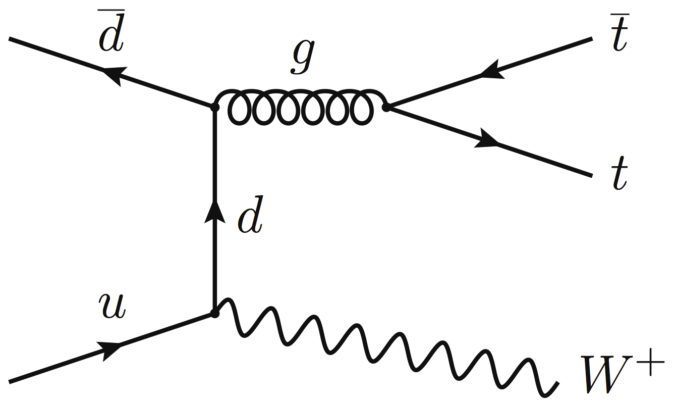
Figure 1: Examples of tree-level Feynman diagrams for $t\bar{t}b\bar{b}$ (left) and $t\bar{t}W$ (right).

2 Comparisons of Monte Carlo predictions for the $t\bar{t}b\bar{b}$ process

In the following section $t\bar{t}b\bar{b}$ background predictions and variations considered to estimate their uncertainties used by ATLAS and CMS in published and future analyses of $t\bar{t}H(H\rightarrow b\bar{b})$ are compared. The first Run-2 $t\bar{t}H(H\rightarrow b\bar{b})$ analyses of both experiments [2, 4] based on partial data sets predicted the $t\bar{t}+jets$ background with a $t\bar{t}$ matrix element (ME) calculated at next-to-leading-order (NLO) accuracy in QCD in the five-flavour scheme (5FS) and matched to the Pythia8 parton shower (PS) [8] in the Powheg framework  [9, 10, 11, 12, 13]. In this set-up, $b$-quarks not originating in the top quark decay chain are produced by Pythia8.

The first predictions using a $t\bar{t}b\bar{b}$ ME at NLO have been performed with stable top quarks in 5FS some time ago [14, 15, 16]. They have been matched subsequently to parton shower programs [17]. Very recently complete calculations for the $t\bar{t}b\bar{b}$ process in di-lepton top quark decay channel have been carried out in 5FS without matching to PS by two independent groups [18, 19, 20]. Such computations are based on $e^{+}\nu_{e}\mu^{-}\overline{\nu}_{\mu}b\overline{b}b\overline{b}$ matrix elements and include all resonant and non-resonant Feynman diagrams, interferences and off-shell effects of the top quark and the W gauge boson.

The first $t\bar{t}H(H\rightarrow b\bar{b})$ analysis based on the full Run-2 data set from ATLAS [1] (”first full Run-2 analysis”) used as nominal generator a calculation where the $t\bar{t}b\bar{b}$ ME is calculated at NLO with massive $b$-quarks in the four-flavour scheme (4FS) [21] and matched to Pythia8 in the Powheg-Box-Res framework [21], referred to as $t\bar{t}b\bar{b}$-Powheg in the following.

For future analyses both experiments consider to use the calculations of $t\bar{t}b\bar{b}$-Powheg matched to Pythia8 as nominal generator however with different settings of the renormalisation and factorisation scale compared to the original paper [21] and slightly different settings of the internal parameters based on more recent studies [22] as will be discussed below.

The estimation of systematic uncertainties differs significantly between the two experiments for the published analyses. ATLAS considered uncertainties due the particular choice of matching algorithm and of the parton shower generator. For the analyses based on partial and first full Run-2 data set, these differences were derived from 5FS $t\bar{t}$ sample predicted by MG5_aMC@NLO [23, 24] matched to Pythia8 for the first and a sample where Powheg is matched to Herwig7 [25] for the latter. Since the nominal generator in the first full Run-2 analysis was based on a $t\bar{t}b\bar{b}$-Powheg calculation, the relative uncertainties derived from the 5FS $t\bar{t}$ samples were used. Uncertainties due to higher order effects were estimated by varying the renormalisation and factorisation scales in the ME, $\mu_{\text{R}}$ and $\mu_{\text{F}}$, simultaneously up and down by a factor of two. Correlations between the scale settings in the ME and $\alpha_{s}$ in the PS ISR were considered by simultaneous variation with $\mu_{\text{R}}$ and $\mu_{\text{F}}$ to cover the effects of PS variations in the presence of matching [26].

In the first Run-2 analysis, CMS considered the uncertainty due to the choice of generator settings by varying the $h_{\text{damp}}$ parameter in Powheg which controls the transverse momentum ($p_{\text{T}}$) of the first additional emission beyond the leading-order Feynman diagram in the PS and therefore regulates the high-$p_{\text{T}}$ emission against which the $t\bar{t}$ system recoils. Comparisons with Sherpa were done internally but not added to the list of systematic uncertainties. The renormalisation and factorisation scales $\mu_{\text{R}}$ and $\mu_{\text{F}}$ as well as $\alpha_{s}$ in both the PS ISR and FSR were varied independently, i.e. one parameter was changed at a time while keeping the other parameters at their nominal values.

For future analyses, both experiments consider predictions with varied $\mu_{\text{R}}$ and $\mu_{\text{F}}$ scales and varied PS $\alpha_{s}$ as well as different settings of $t\bar{t}b\bar{b}$-Powheg internal parameters, however ATLAS studies additional uncertainties due to parton shower and matching. To estimate the dependence on $t\bar{t}b\bar{b}$-Powheg internal parameters, ATLAS varies the parameter $h_{\text{bzd}}$ which regulates the splitting into the finite and the singular part of the real emission in the Powheg framework. Variations of the parameter $h_{\text{damp}}$ were studied in Ref. [22] but no significant differences were found and therefore this variation is not further considered for uncertainty estimates. Uncertainties due to the particular setting of PS are estimated with set-ups of $t\bar{t}b\bar{b}$-Powheg matched to Herwig7 and Pythia8 with a dipole recoil. The dependence on the particular choice of generator and the NLO matching algorithm is studied by comparing to NLO 4FS predictions of $t\bar{t}b\bar{b}$ generated with Sherpa 2.2.10 [27, 28, 29]. Details of the studies are given in Ref. [22].

In case of CMS, the dependence on $t\bar{t}b\bar{b}$-Powheg internal parameters is estimated by varying the matching parameter $h_{\text{damp}}$.

Both experiments consider PDF uncertainties in the published and future analyses, however they are neglected in the studies presented here due to the smallness of the effect. Finally, in order to get comparable results, the scale uncertainties are treated the same way for both experiments in all studies presented here, i.e.  $\mu_{\text{R}}$ and $\mu_{\text{F}}$, PS ISR and PS FSR are changed individually by a factor 0.5 (2) while keeping the other parameters at their nominal values.

All comparisons are performed using stable final-state particles in a fiducial phase space similar to the experimental measurements implemented in a dedicated routine in the Rivet analysis toolkit [7, 30].

The chapter is organised as follows. Section 2.1 describes the samples used for the comparison and the technical set-up of their generation. Section 2.2 describes the observables and the fiducial phase space used for the comparison and finally, Sec. 2.3 displays the resulting comparisons.

2.1 MC generator set-ups

The set-ups used to generate $t\bar{t}b\bar{b}$ predictions with $t\bar{t}b\bar{b}$-Powheg, Powheg, MG5_aMC@NLO and Sherpa are described in the following. The generator configurations and version numbers are summarised in Table 1 and their scale settings are given in Table 2. The systematic uncertainty estimates due to scale and $\alpha_{s}$ variations are summarised in Table 3.

The $b$-quark mass is set to $4.75\text{\,}\mathrm{GeV}$ for CMS samples and for Sherpa, and to $4.95\text{\,}\mathrm{GeV}$ for all other ATLAS samples. The top quark mass is set to $172.5\text{\,}\mathrm{GeV}$. The decay of the top quark is calculated by the corresponding generators (Powheg, Sherpa) respecting the spin correlation. The PDF sets used in the ME calculation are selected from the NNPDF family for all samples, where ATLAS uses version 3.0 while CMS uses version 3.1. The ATLAS $t\bar{t}b\bar{b}$-Powheg, Powheg and MG5_aMC@NLO samples use EvtGen [31] for simulation of the $B$-hadron decays, while the Sherpa sample and all CMS samples calculate the decays within the corresponding PS codes. All samples were produced for final states with one or two leptons.

$t\bar{t}b\bar{b}$-Powheg samples:

Nominal $t\bar{t}b\bar{b}$ predictions are calculated using the Powheg-Box-Res framework at NLO with massive $b$-quarks [21] with the “4FS NLO as 0118” PDF sets. The renormalisation scale is set to half of the geometric average of the transverse mass of top- and $b$-quarks defined as $m_{\text{T},i}=\sqrt{m^{2}_{i}+p^{2}_{\text{T},i}}$, where $m_{i}$ refers to the mass, $p_{\text{T},i}$ to the transverse momentum and $i$ to the top or $b$-quark. The factorisation scale is related to the average of the transverse mass of the outgoing partons in the ME calculation, see Table 2. For ATLAS, it follows Ref. [21], while it is set to a factor two smaller in CMS following Ref. [32]. The $t\bar{t}b\bar{b}$-Powheg internal parameters differ between the experiments: $h_{\text{bzd}}$ is set to 5 for ATLAS and to 2 for CMS, $h_{\text{damp}}$ is set to $H_{\text{T}}$/2 for ATLAS and to 1.379 times the top quark mass for CMS. The Pythia8 parameters for PS and hadronisation modelling are set to the A14 [33] and CP5 [34] tunes for ATLAS and CMS and the samples are referred to as ATLAS and CMS PP8 $t\bar{t}b\bar{b}$ samples, respectively.

To vary $t\bar{t}b\bar{b}$-Powheg internal parameters, ATLAS sets the parameter $h_{\text{bzd}}$ to 2. CMS varies in its set-up the $h_{\text{damp}}$ parameter to 2.305 times the top quark mass for the “$h_{\text{damp}}$ up” variation and to 0.8738 times the top quark mass for the “$h_{\text{damp}}$ down” variation.

The ATLAS $t\bar{t}b\bar{b}$-Powheg calculation was performed using a special option where virtual corrections are switched off and then reweighted with virtual corrections switched on, while the CMS samples used default calculation.

For the PS variations, ATLAS uses the set of LHE files which store the results of the ME calculation by $t\bar{t}b\bar{b}$-Powheg for the PP8 $t\bar{t}b\bar{b}$ sample and matches them to a different PS prediction. For the prediction with the Pythia8 dipole shower only the treatment of the recoil of the radiated parton in the shower is changed and all other parameters are kept as the A14 tuned values. Another sample is produced where Herwig7 is used with the default tune provided with this generator version.

Sherpa $t\bar{t}b\bar{b}$ samples:

A $t\bar{t}b\bar{b}$ sample was generated using Sherpa version 2.2.10 [27, 28, 29]. The $t\bar{t}b\bar{b}$ MEs were calculated with massive $b$-quarks at NLO, using the COMIX [35] and Openloops [29] ME generators, and merged with the Sherpa PS, tuned by the authors [36]. The same renormalisation and factorisation scales and PDFs are used as for the ATLAS PP8 $t\bar{t}b\bar{b}$ prediction.

Inclusive $t\bar{t}$ samples:

The inclusive $t\bar{t}$ samples are generated with the Powheg v2 NLO event generator [9, 10, 12, 13, 37] and MG5_aMC@NLO using a 5FS PDF set. The renormalisation and factorisation scales were set to the average transverse mass of the top quark and antiquark.

For the Powheg samples of both experiments, the PS and hadronisation is modeled by Pythia8 with the same versions and settings as for the PP8 $t\bar{t}b\bar{b}$ samples above. The $h_{\text{damp}}$ parameter was set to the 1.5 times the top quark mass for ATLAS and to 1.379 times the top quark mass for CMS. Another ATLAS sample is generated using Herwig7 for the PS and hadronization. These samples are referred to as ATLAS (CMS) PP8 $t\bar{t}$ and ATLAS PH7 $t\bar{t}$ samples.

The inclusive MG5_aMC@NLO $t\bar{t}$ sample uses the same scale settings and the same Pythia8 version as the ATLAS PP8 $t\bar{t}$ sample and is referred to as ATLAS aMC+P8 $t\bar{t}$ sample.

Table 1: Configurations used for the event generation of the $t\bar{t}b\bar{b}$ process and the predicted total cross section for events with at least one lepton.

	name	ME	Generator	ME order	Shower	Tune	NNPDF PDF set (ME)	$h_{\text{damp}}$	$h_{\text{bzd}}$	$\sigma^{\geq 1\text{lep}}$ [$\mathrm{pb}$]
ATLAS	PP8 $t\bar{t}b\bar{b}$	$t\bar{t}b\bar{b}$	$t\bar{t}b\bar{b}$-Powheg	NLO	Pythia 8.224	A14	4FS 3.0 NLO as 0118	$H_{T}/2$	5	18.72
CMS	PP8 $t\bar{t}b\bar{b}$	$t\bar{t}b\bar{b}$	$t\bar{t}b\bar{b}$-Powheg	NLO	Pythia 8.230	CP5	4FS 3.1 NLO as 0118	$1.379\cdot m_{t}$	2	23.86
ATLAS	PP8 $t\bar{t}b\bar{b}$ $h_{\text{bzd}}$ 2	$t\bar{t}b\bar{b}$	$t\bar{t}b\bar{b}$-Powheg	NLO	Pythia 8.224	A14	4FS 3.0 NLO as 0118	$H_{\text{T}}/2$	2	18.46
ATLAS	PP8 $t\bar{t}b\bar{b}$ dipole	$t\bar{t}b\bar{b}$	$t\bar{t}b\bar{b}$-Powheg	NLO	Pythia 8.224	A14, dipoleRecoil	4FS 3.0 NLO as 0118	$H_{\text{T}}/2$	2	18.72
ATLAS	PH7 $t\bar{t}b\bar{b}$	$t\bar{t}b\bar{b}$	$t\bar{t}b\bar{b}$-Powheg	NLO	Herwig 7.1.6	default	4FS 3.0 NLO as 0118	$H_{\text{T}}/2$	5	18.47
ATLAS	Sherpa $t\bar{t}b\bar{b}$	$t\bar{t}b\bar{b}$	Sherpa 2.2.10	NLO	Sherpa	default	4FS 3.0 NNLO as 0118	—	—	20.24
CMS	PP8 $t\bar{t}b\bar{b}$ $h_{\text{damp}}$ up	$t\bar{t}b\bar{b}$	$t\bar{t}b\bar{b}$-Powheg	NLO	Pythia 8.230	CP5	4FS 3.1 NLO as 0118	$2.305\cdot m_{t}$	5	23.86
CMS	PP8 $t\bar{t}b\bar{b}$ $h_{\text{damp}}$ down	$t\bar{t}b\bar{b}$	$t\bar{t}b\bar{b}$-Powheg	NLO	Pythia 8.230	CP5	4FS 3.1 NLO as 0118	$0.8738\cdot m_{t}$	5	23.86
ATLAS	PP8 $t\bar{t}$	$t\bar{t}$	Powheg v2	NLO	Pythia 8.210	A14	5FS 3.0 NLO	$1.5\cdot m_{t}$	5	451.78
CMS	PP8 $t\bar{t}$	$t\bar{t}$	Powheg v2	NLO	Pythia 8.230	CP5	5FS 3.1 NLO	$1.5\cdot m_{t}$	5	451.78c
ATLAS	PH7 $t\bar{t}$	$t\bar{t}$	Powheg v2	NLO	Herwig 7.13	default	5FS 3.0 NLO	$1.5\cdot m_{t}$	5	451.78c
ATLAS	aMC+P8 $t\bar{t}$	$t\bar{t}$	MG5_aMC@NLO	NLO	Pythia 8.210	A14	5FS 3.0 NLO	—	—	451.78c
CMS	PP8 $t\bar{t}$ $h_{\text{damp}}$ up	$t\bar{t}$	Powheg v2	NLO	Pythia 8.230	CP5	5FS 3.1 NLO	$2.305\cdot m_{t}$	5	451.78c
CMS	PP8 $t\bar{t}$ $h_{\text{damp}}$ down	$t\bar{t}$	Powheg v2	NLO	Pythia 8.230	CP5	5FS 3.1 NLO	$0.8738\cdot m_{t}$	5	451.78c

Table 2: Scale choices used in the event generation of $t\bar{t}b\bar{b}$ and $t\bar{t}$ processes for the different generators.

ME Generator	$\mu_{\text{R}}$	$\mu_{\text{F}}$
ATLAS $t\bar{t}b\bar{b}$-Powheg $t\bar{t}b\bar{b}$	$\frac{1}{2}\sqrt[4]{m_{\text{T},t}\cdot m_{\text{T},\bar{t}}\cdot m_{\text{T},b}\cdot m_{\text{T},\bar{b}}}$	$\frac{1}{2}(m_{\text{T},t}+m_{\text{T},\bar{t}}+m_{\text{T},b}+m_{\text{T},\bar{b}}+m_{\text{T},g})$
CMS $t\bar{t}b\bar{b}$-Powheg $t\bar{t}b\bar{b}$	$\frac{1}{2}\sqrt[4]{m_{\text{T},t}\cdot m_{\text{T},\bar{t}}\cdot m_{\text{T},b}\cdot m_{\text{T},\bar{b}}}$	$\frac{1}{4}(m_{\text{T},t}+m_{\text{T},\bar{t}}+m_{\text{T},b}+m_{\text{T},\bar{b}}+m_{\text{T},g})$
Sherpa 2.2.10	$\frac{1}{2}\sqrt[4]{m_{\text{T},t}\cdot m_{\text{T},\bar{t}}\cdot m_{\text{T},b}\cdot m_{\text{T},\bar{b}}}$	$\frac{1}{2}(m_{\text{T},t}+m_{\text{T},\bar{t}}+m_{\text{T},b}+m_{\text{T},\bar{b}}+m_{\text{T},g})$
ATLAS Powheg $t\bar{t}$	$\sqrt{0.5\cdot(m_{\text{T},t}^{2}+m_{\text{T},\bar{t}}^{2})}$	$\sqrt{0.5\cdot(m_{\text{T},t}^{2}+m_{\text{T},\bar{t}}^{2})}$
CMS Powheg $t\bar{t}$	$\sqrt{0.5\cdot(m_{\text{T},t}^{2}+m_{\text{T},\bar{t}}^{2})}$	$\sqrt{0.5\cdot(m_{\text{T},t}^{2}+m_{\text{T},\bar{t}}^{2})}$
ATLAS aMC $t\bar{t}$	$\sqrt{0.5\cdot(m_{\text{T},t}^{2}+m_{\text{T},\bar{t}}^{2})}$	$\sqrt{0.5\cdot(m_{\text{T},t}^{2}+m_{\text{T},\bar{t}}^{2})}$

Table 3: Systematic variations of scales in the ME and PS codes used for all comparisons presented here.

Variation
Scale variation ME	$\mu_{\text{R}}$ $\times$ 0.5, $\mu_{\text{F}}$ $\times$ 0.5; $\mu_{\text{R}}$ $\times$ 2, $\mu_{\text{F}}$ $\times$ 2
ISR variation (PS)	$\alpha_{\text{s}}^{\text{ISR}}\times 0.5;{\alpha_{\text{s}}}^{\text{ISR}}\times 2.0$
FSR variation (PS)	$\alpha_{\text{s}}^{\text{FSR}}\times 0.5;{\alpha_{\text{s}}}^{\text{FSR}}\times 2.0$

2.2 Object reconstruction, fiducial volume and observables

The object definition and event selection applied in this comparison study is defined at particle level and is the same for ATLAS and CMS. All objects are defined using stable final-state particles with a mean lifetime of $\tau>$3\text{\times}{10}^{-11}\text{\,}\mathrm{s}$$. Jets are reconstructed from all stable final-state particles (but excluding leptons and neutrinos from the top quark decay chain) using the anti-$k_{\mathrm{t}}$ jet algorithm [38, 39] with a radius parameter of $R=0.4$. Jets which contain at least one ghost-associated [40] $B$-hadron with $p_{\text{T}}>$5\text{\,}\mathrm{GeV}$$ are defined as $b$-jets, all other jets are considered “light” jets. The four-momentum of the bare leptons from top quark decay are modified (“dressed”) by adding the four-momenta of all radiated photons within a cone of size $\Delta R=0.1$. All objects are considered within pseudo-rapidity $|\eta|<2.5$ and with $p_{\text{T}}>$27\text{\,}\mathrm{GeV}$$ for leptons and $p_{\text{T}}>$25\text{\,}\mathrm{GeV}$$ for jets and $b$-jets.

Leptons are removed if they are separated from a jet by less than $\Delta R=0.4$, where $\Delta R=\sqrt{(\Delta\eta)^{2}+(\Delta\phi)^{2}}$. Events are selected with at least four $b$-jets, and further separated into two analysis regions: events with exactly one lepton and at least six jets (single lepton channel) and events with exactly two leptons and at least four jets (dilepton channel).

A set of observables relevant for the $t\bar{t}H(H\rightarrow b\bar{b})$ analysis is studied within this fiducial phase space. All observables are studied for both the single lepton and the dilepton channel, however only the variables listed in Table 4 are shown in the following figures, as no significant qualitative difference is observed between the different top quark decay channels.

Table 4: The list of observables used for the comparison of the generators for the $t\bar{t}b\bar{b}$ process.

Variable	Description	Channel
$\Delta R_{bb}^{\text{min}\Delta R}$	$\Delta R$ of the two $b$-jets in the event which are closest in $\Delta R$	dilepton
$m_{bb}^{\text{min}\Delta R}$	Invariant mass of the two $b$-jets closest in $\Delta R$	dilepton
$N_{\text{jets}}$	Number of jets in the event (all jet flavours)	dilepton
Light jet $p_{\text{T}}$	Transverse momentum of the light jets in the event	dilepton
$N_{\text{$b$-jets}}$	Number of $b$-jets in the event	single lepton
$H_{\text{T}}^{\text{jets}}$	Scalar sum of $p_{\text{T}}$ of jets in the event (all jet flavours)	single lepton
Leading $b$-jet $p_{\text{T}}$	$p_{\text{T}}$ of $b$-jet with largest $p_{\text{T}}$ in the event	single lepton
Fourth $b$-jet $p_{\text{T}}$	$p_{\text{T}}$ of $b$-jet with fourth largest $p_{\text{T}}$ in the event	single lepton

2.3 Results

Three sets of generator predictions are compared for the observables given in Table 4 as follows. All comparisons are performed with respect to the $t\bar{t}b\bar{b}$ PP8 sample. The PP8 $t\bar{t}b\bar{b}$ sample and the alternative predictions are normalised to an integral of one, after all selections and in each histogram individually for a shape-only comparison. The scale uncertainty variations on PP8 $t\bar{t}b\bar{b}$ are derived as listed in Table 3 and the differences are added in quadrature to the statistical uncertainties to form the shaded area displayed in the figures.

Figure 2 shows the nominal $t\bar{t}b\bar{b}$ predictions from ATLAS and CMS to be used in future analyses compared to the nominal predictions used in the early Run-2 analyses. The differences between ATLAS and CMS set-ups cause only minor differences between the predictions. However, significant differences between the PP8 $t\bar{t}b\bar{b}$ predictions and the PP8 $t\bar{t}$ predictions are observed in $\Delta R_{b\bar{b}}^{\text{min}\Delta R}$, the jet multiplicity and in the number of events with more than four $b$-jets. Furthermore, the uncertainty band is slightly larger in the CMS $t\bar{t}b\bar{b}$ predictions, potentially caused by the lower factorisation scale.

In Fig. 3, the ATLAS nominal PP8 $t\bar{t}b\bar{b}$ prediction is compared to all generator variations potentially considered as modelling uncertainties for future ATLAS $t\bar{t}H(H\rightarrow b\bar{b})$ analyses, i.e. variations in $t\bar{t}b\bar{b}$-Powheg and Pythia8 parameter settings as well as Sherpa as alternative generator. As already discussed in Ref. [22], the parameter $h_{\text{bzd}}$ has only a minor influence on the observables. Interestingly, predictions of $t\bar{t}b\bar{b}$-Powheg matched to Pythia8 using the dipole shower and matched to the Herwig7 PS both show a significant decrease with respect to the nominal PP8 $t\bar{t}b\bar{b}$ in the jet multiplicity and $H_{\text{T}}$. Sherpa differs up to 10–20 % in all distributions with significant differences in shape.

In Fig. 4, the CMS nominal PP8 $t\bar{t}b\bar{b}$ prediction is compared to generator variations potentially considered for the CMS $t\bar{t}H(H\rightarrow b\bar{b})$ analysis. The scale uncertainties, which include the scale variations in the ME and the PS, are significantly larger than the differences observed for the different $h_{\text{damp}}$ variations, except at very low $H_{\text{T}}$ and low leading $b$-jet $p_{\text{T}}$ where the $h_{\text{damp}}$ down variations shows up to 20 % differences. Significant statistical fluctuations are observed at regions of low event yields, which are, however, not expected to be relevant for the analysis.

Finally, Fig. 5 shows the distributions used to estimate the systematic modelling uncertainties of the first Run-2 analysis by CMS [4] and of the first full Run-2 analysis by ATLAS [1]. In addition to the scale and PS $\alpha_{s}$ variations, the uncertainty on the $t\bar{t}b\bar{b}$ PP8 prediction is estimated in case of ATLAS by assigning the relative difference between PP8 $t\bar{t}$ and alternative $t\bar{t}$ predictions listed in Table 1 to the $t\bar{t}b\bar{b}$ prediction, and in case of CMS by the $h_{\text{damp}}$ variations, where also a cross check with Sherpa $t\bar{t}$ has been made but was not included in the fit. Due to displaying purposes, the ATLAS PP8 $t\bar{t}$ prediction, which is very similar to the CMS $t\bar{t}$ prediction as demonstrated in Fig. 2, is not shown.

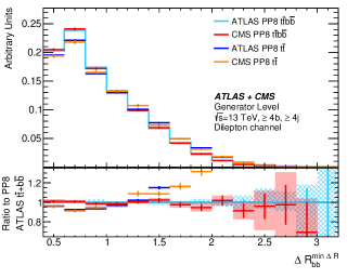
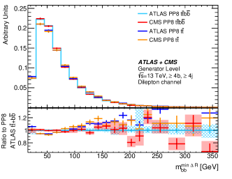
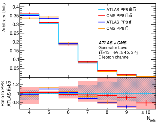
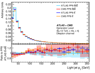
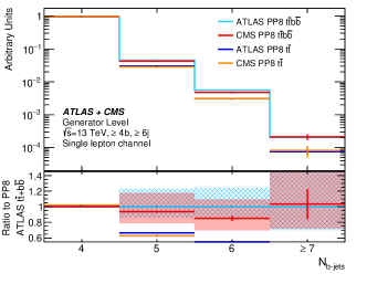
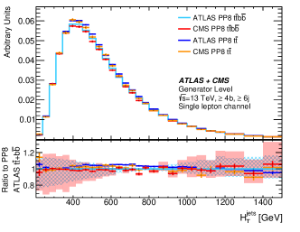
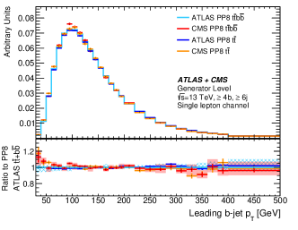
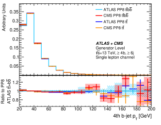
Figure 2: Comparison of PP8 predictions for $t\bar{t}b\bar{b}$ and $t\bar{t}$ with the described settings using the observables defined in Table 4 in the fiducial analysis phase space. All predictions are normalised to one. The error bands are constructed from the statistical uncertainties and the scale variations (ME and PS) for the ATLAS PP8 $t\bar{t}b\bar{b}$ (blue) and the CMS PP8 $t\bar{t}b\bar{b}$ (red) samples. Statistical uncertainties are indicated by vertical lines. The ratio shows the different curves divided by the ATLAS PP8 $t\bar{t}b\bar{b}$ prediction.

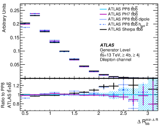
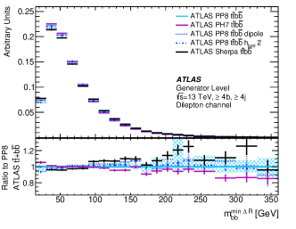
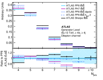
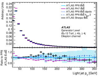
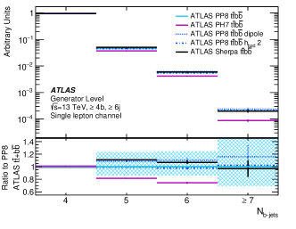
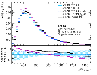
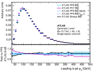
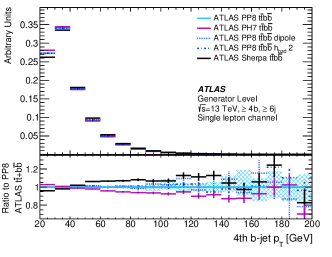
Figure 3: Comparison of ATLAS PP8 predictions for $t\bar{t}b\bar{b}$ with different matching and PS settings and Sherpa. All distributions are normalised to one. The ratio shows the different curves divided by PP8 $t\bar{t}b\bar{b}$. The error band contains the statistical uncertainty and the scale variations (ME and PS) for the ATLAS PP8 $t\bar{t}b\bar{b}$ sample. Statistical uncertainties are indicated by vertical lines.

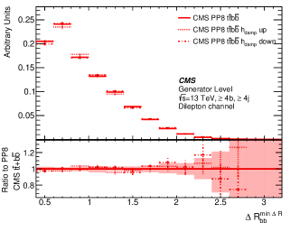
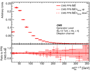
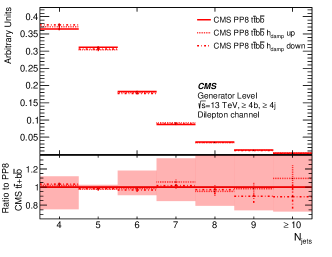
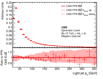
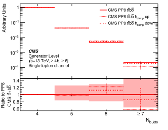
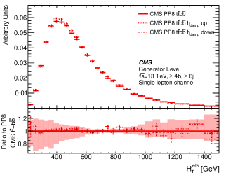
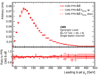
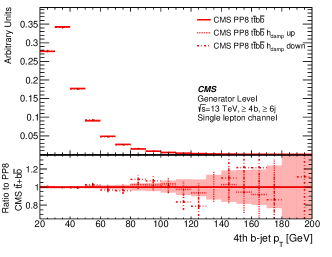
Figure 4: Comparison of CMS PP8 predictions for $t\bar{t}b\bar{b}$ with different settings of the parameter $h_{\text{damp}}$. All predictions are normalised to one. The ratio shows the different curves divided by PP8 $t\bar{t}b\bar{b}$. The error band contains the statistical uncertainty and the scale variations (ME and PS) for the CMS PP8 $t\bar{t}b\bar{b}$ sample. Statistical uncertainties are indicated by vertical lines.

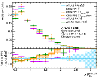
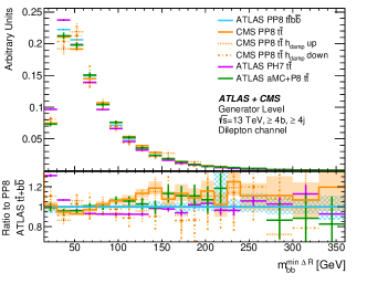
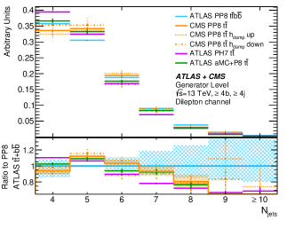
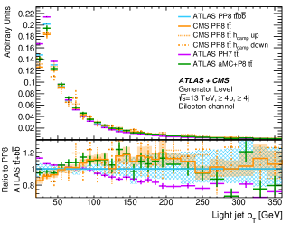
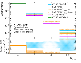
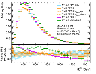
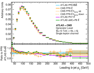
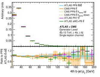
Figure 5: Comparison of predictions used for the systematic uncertainties of the first Run-2 analysis by CMS [4] and of the first full Run-2 analysis by ATLAS [1]. All distributions are normalised to one. The ratio shows the different curves divided by ATLAS PP8 $t\bar{t}b\bar{b}$. The error bands are constructed from the statistical uncertainties and the scale variations (ME and PS) for the ATLAS PP8 $t\bar{t}b\bar{b}$ (blue) and the CMS PP8 $t\bar{t}b\bar{b}$ (red) samples. Statistical uncertainties are indicated by vertical lines.

2.4 Conclusions

Comparisons of generator predictions used by ATLAS and CMS in a typical phase space of the $t\bar{t}H(H\rightarrow b\bar{b})$ measurement were presented. Two sets are used for comparison: the generators used in the most recent published analyses involving $t\bar{t}$ inclusive predictions based on 5FS PDFs to estimate uncertainties and the set of generators in the future effort using $t\bar{t}b\bar{b}$ calculations at NLO based on 4FS PDFs.

The difference between the predictions exceeds the uncertainties from the scale variations both for the uncertainties considered in the published $t\bar{t}H(H\rightarrow b\bar{b})$ analysis and for the future analyses. The uncertainties due to the choice of PS and NLO generator are reduced when estimating them based on $t\bar{t}b\bar{b}$ ME predictions compared to the previously used $t\bar{t}$ ME matched predictions.

Despite differences in the set-ups between the experiments for the nominal PP8 $t\bar{t}b\bar{b}$ generator, only small differences are observed in the predictions. However, the considerations of the modelling uncertainties differs significantly: CMS considers inherent variations of the chosen model as uncertainty, while ATLAS studied inherent variations and differences obtained with alternative generator choices and the latter dominates the uncertainties. Scale variations are applied by both experiments, however the details of the estimates differ between ATLAS and CMS in the published analysis but the effect of the different treatment are not yet studied for the future analyses.

The presented studies shall be used as input to discussions between the experiments and theorists to define theory uncertainties for future combinations of ATLAS and CMS.

3 Comparisons of Monte Carlo predictions for the $t\bar{t}W$ process

The ATLAS [5] and CMS [6] experiments measured the $t\bar{t}H$ production cross section in multi-lepton final states, which are primarily sensitive to the decays of $H\rightarrow WW^{*}$, $H\rightarrow\tau\tau$ and $H\rightarrow ZZ^{*}$. The dominant background in these measurements stems from $t\bar{t}W$ production. These measurements along with the recent CMS measurement of $t\bar{t}W$ production [41] show some tension with the SM $t\bar{t}W$ predictions which were used to calculate the inclusive cross section and the acceptance in the analysis phase space.

Different nominal MC predictions were used by the experiments for these measurements, ATLAS used Sherpa 2.2.1 [27] and CMS used MG5_aMC@NLO 2.4.2 matched to Pythia8 using the FxFx merging scheme [24] and including sub-leading electroweak (EW) corrections of the order $\alpha_{s}\alpha^{3}$ where $\alpha$ ($\alpha_{s}$) refers to the EW (QCD) coupling constant. The experiments applied different corrections to predict the theoretical inclusive $t\bar{t}W$ cross section that entered the calculation of the scale factor to data, resulting in a value of $727\text{\,}\mathrm{fb}$ for ATLAS [5] and $650\text{\,}\mathrm{fb}$ for CMS [6]. Both experiments estimate the uncertainty of the MC prediction related to missing higher order corrections by varying the renormalisation and factorisation scales in the ME. However, ATLAS considers additionally uncertainties associated with the modelling of additional QCD radiation by comparing the nominal $t\bar{t}W$ prediction with that of MG5_aMC@NLO+Pythia8 as alternative MC generator differing in particular in the number of additional partons in the ME calculation, the parton shower and merging algorithm.

In recent times there have been significant theoretical developments in $t\bar{t}W$ modelling despite the challenges associated with calculations of $t\bar{t}W$ with higher order corrections in the QCD, $\alpha_{s}$, and EWK, $\alpha$, couplings. Even at LO in $\alpha_{s}$, complications arise because $t\bar{t}W$ is a $q\overline{q}$-initiated process in which the radiation of the $W$-boson from one of the initial state quarks polarises the incoming quark, making spin correlations all the more important [42]. Initial calculations of $t\bar{t}W$ production at next-to-leading order (NLO) in QCD at fixed order [43] and later matched to a parton shower [44, 45] were later augmented with NLO EWK corrections (of order $\alpha^{2}\alpha_{s}^{2}$) [46] to provide the higher order cross sections used across the LHC programme for a number of years [47]. Furthermore, full NLO calculations including fixed-order corrections matched to parton shower in the POWHEG-BOX framework and accounting for LO spin-correlation of decay product have recently been provided in [48].

Since then there has been significant theoretical progress in calculating more complex and precise predictions. Higher order QCD corrections including $t\bar{t}W$ production with additional partons open gluon-initiated production modes with significant contributions to the total cross section. Recent studies show that these contributions also have large next-to-leading order (NLO) corrections [23] and that $t\bar{t}W$ $jj$ can be large [49], both of which require NLO-merged calculations [50] for such effects to be properly included. Furthermore, beyond the traditionally “leading” NLO EWK corrections (of order $\alpha^{2}\alpha_{s}^{2}$) there are even larger contributions from traditionally “sub-leading” NLO corrections (of order $\alpha^{3}\alpha_{s}$) [51, 52, 48] due to the existence of $tW$ scattering contributions embedded in to the $t\bar{t}W$$j$ process. Calculations at NLO in QCD accounting for next-to-next-to-leading logarithmic effects (NNLL) are also available [53] as well as recent predictions at NLO+NNLL in QCD also with NLO EWK corrections [54, 55]. Full off-shell calculations at NLO in QCD [56, 57, 58] are also now available and more recently the NLO EWK corrections have also been incorporated [59] into these calculations, along with the development of procedures to apply the off-shell corrections to NLO+PS setups [60].

A first attempt to formulate an uncertainty estimate in view of these theoretical predictions has been made in [48] where different generator codes at NLO QCD are compared with fixed order calculations to demonstrate that a robust theoretical prediction of hadronic $t\bar{t}W$ production cannot be expressed as a simple recipe covering the specifics of all experimental observables. Therefore the value of comparing several well tested tools is emphasised.

For future analyses, updated MC models will be used and the estimate of systematic uncertainty is under development. In particular, ATLAS is considering Sherpa predictions including several higher order EW corrections in addition to the predictions at NLO in the strong coupling, namely of the order $\alpha^{3}$, $\alpha^{2}\alpha_{s}^{2}$ and $\alpha^{3}\alpha_{s}$. Furthermore, calculations of MG5_aMC@NLO+Pythia8 employing the FxFx merging scheme will be considered. For inclusive predictions, Powheg predictions [48] are also considered. CMS will continue to use MG5_aMC@NLO+Pythia8 with the FxFx merging scheme including subleading EW corrections however the EW corrections are not included in the present document in order to facilitate the comparison between the setups used by each experiment. The samples will be described in the following and an overview with detailed information on the samples is given in Table 5. The use of other theoretical developments, already outlined, will also be considered in future but are beyond the scope of this document.

Comparisons are performed using stable final-state particles in a fiducial phase space similar to the experimental measurements in the two same-sign leptons (2lSS) channel as implemented in a dedicated routine in the Rivet analysis toolkit [7]. Two sets of distributions are presented, one where the histograms are normalised to unit area to asses shape differences in the differential distributions and another set where the generator cross sections are set to $600.8\text{\,}\mathrm{fb}$ the value reported in Ref. [47]. This allows to study differences in acceptance for the different generator predictions.

The chapter is organised as follows: Section 3.1 gives the detailed set-up for the generator samples, Section 3.2 describes the object reconstruction and event selection, Section 3.3 gives the two sets of results and finally conclusions are drawn in Section 3.4.

3.1 MC generator set-ups

This chapter describes in detail the set-up of the MC generator set-ups used for the ATLAS and CMS samples.

ATLAS setup

The nominal sample for the comparison of this note was generated using the Sherpa 2.2.10 [27, 61] generator with the NNPDF3.0 NLO PDF set. The $t\bar{t}W$ matrix element was calculated for up to one additional parton at NLO and up to two partons at leading order (LO) accuracy using Comix [35] and OpenLoops [29], and merged with the Sherpa parton shower [36] using the MEPs@NLO prescription [62] with a merging scale of $30\text{\,}\mathrm{GeV}$. The choice of renormalisation and factorisation scales of the core process is $\mu_{\text{R}}=\mu_{\text{F}}=H_{\text{T}}/2$, where $H_{\text{T}}$ is defined as the scalar sum of the transverse masses $\sqrt{p_{\text{T}}^{2}+m^{2}}$ of all final state particles. Systematic uncertainties due to missing higher-order QCD corrections are estimated in the nominal sample by varying the factorisation and renormalisation scales together with $\alpha_{s}$ in the parton shower by a factor of 0.5 (2.0) with respect to the central value.

In addition to this nominal prediction at NLO in the strong coupling, a separate sample is produced which contains also higher order corrections relating to EW contributions. These are added in two ways. First, event-by-event correction factors are applied that provide virtual NLO EW corrections of the order $\alpha^{2}\alpha_{s}^{2}$ derived using the formalism described in Ref. [63] along with LO corrections of order $\alpha^{3}$, both are implemented using the prescription outlined in Refs. [27, 64]. Second, sub-leading EW corrections at order $\alpha^{3}\alpha_{s}$ [52] are partially accounted for (only the real emission contribution) via the addition of an independent Sherpa 2.2.10 sample produced at LO in QCD for this final state. This sample is marked as “QCD+EW” in the following.

Alternative $t\bar{t}W$ predictions are produced using the MG5_aMC@NLO 2.3.3 program to generate $t\bar{t}W$ production with up to one additional parton in the final state at NLO accuracy in the strong coupling. The renormalisation and factorisation scales are the same as in the nominal sample. Another sample is generated using MG5_aMC@NLO 2.9.3 for up to one additional parton at NLO accuracy and up to two additional partons at LO accuracy in the ME and merging the different jet multiplicities using the FxFx NLO matrix-element and parton-shower merging prescription [24], see detailed description in [65]. As part of the FxFx merging algorithm, scales are dynamically chosen and set to the characteristic scale of the hard process. In both samples, spin correlation effects between the ME decay products are accounted for by Madspin [66] and the showering and subsequent hadronization is performed using Pythia 8.210 and Pythia 8.245 [8], respectively, with the A14 tune [33]. These samples are referred to as “ATLAS MG5_aMC+Py8” and “ATLAS MG5_aMC+Py8 FxFx” in the following.

CMS setup

CMS simulates proton-proton to $t\bar{t}\ell\nu$ processes at NLO accuracy in the matrix element calculation using MG5_aMC@NLO 2.4.2. Spin correlation effects between the ME decay products are accounted for by Madspin [66]. The ME calculation includes diagrams with up to one additional parton at NLO and any further partons are generated by the parton shower. The renormalisation and factorisation scales are set to the characteristic scale of the hard process. They are chosen dynamically and are dependent kinematics of the event after the FxFx merging prescription.

Theoretical uncertainties associated with missing higher-order QCD corrections from the ME calculation are estimated by varying the renormalisation and factorisation scale by a factor of 0.5 and 2.0. All possible combinations of these variations, implemented using a dedicated set of per-event weights, are then used to construct the uncertainty envelope.

The parton shower, hadronization processes and decays of $\tau$  leptons (including polarisation effects) are modelled using Pythia 8.226 with the CP5 tune. The samples is called “CMS MG5_aMC+Py8 FxFx” in the following.

Table 5: The configurations used for the event generation of the $t\bar{t}W$ processes. Scale settings given in terms of $H_{\text{T}}=\sum_{i=0}^{N}\sqrt{p_{T,i}^{2}+m_{i}^{2}}$, where N corresponds to the number of final state particles.

Label	ATLAS Sherpa 2.2.10	ATLAS Sherpa 2.2.10	ATLAS MG5_aMC+Py8 FxFx	ATLAS MG5_aMC+Py8	CMS MG5_aMC+Py8 FxFx
		QCD+EW
Process	$t\bar{t}W$ inclusive	$t\bar{t}W$ inclusive	$t\bar{t}W$ inclusive	$t\bar{t}W$ inclusive	$t\bar{t}\ell\nu$ ($t\bar{t}W$ inclusive)
Generator	Sherpa 2.2.10 [27]	Sherpa 2.2.10 [27]	MG5_aMC@NLO 2.9.3 [69]	MG5_aMC@NLO 2.3.3 [70]	MG5_aMC@NLO 2.4.2
order of QCD ME	0,1 $j$@NLO	0,1 $j$@NLO	0,1 $j$@NLO	NLO	0,1 $j$@NLO
ME or core scale	$\mu_{\text{R}}=\mu_{\text{F}}=H_{\text{T}}/2$	$\mu_{\text{R}}=\mu_{\text{F}}=H_{\text{T}}/2$	dynamic scale choice [24, 67, 68]	$\mu_{\text{R}}=\mu_{\text{F}}=H_{\text{T}}/2$	dynamic scale choice [24, 67, 68]
order of EW corr.	-	$\alpha^{3}$, $\alpha^{2}\alpha_{s}^{2}$, $\alpha^{3}\alpha_{s}$	-	-	-
Parton Shower	Sherpa 2.2.10	Sherpa 2.2.10	Pythia 8.245 [8]	Pythia 8.210 [8]	Pythia 8.226
Merging Scheme	MEPs@NLO [62]	MEPs@NLO [62]	FxFx [24]	-	FxFx
Merging Scale	$30\text{\,}\mathrm{GeV}$	$30\text{\,}\mathrm{GeV}$	$30\text{\,}\mathrm{GeV}$	-	$42\text{\,}\mathrm{GeV}$
PDF	NNPDF3.0 NNLO [71]	NNPDF3.0 NNLO	NNPDF3.0 NLO	NNPDF3.0 NLO	NNPDF3.1 NLO [72]
Tune	Sherpa default	Sherpa default	A14 [33]	A14	CP5 [34]
Cross section	$597\text{\,}\mathrm{fb}$	$615\text{\,}\mathrm{fb}$	$613\text{\,}\mathrm{fb}$	$548\text{\,}\mathrm{fb}$	$220\text{\,}\mathrm{fb}$ (666 fb)

3.2 Object reconstruction, fiducial volume and observables

Object and event selection is defined at stable particle-level that closely matches the detector-level described in reference [5] (ATLAS) and [6] (CMS). Jets are reconstructed from all stable final state particles with a mean lifetime of $\tau>$3\text{\times}{10}^{-11}\text{\,}\mathrm{s}$$ (but excluding leptons and neutrinos from the top quark decay chain), using the anti-$k_{t}$ algorithm with a radius parameter of $R=0.4$. Jets are required to satisfy $p_{\text{T}}>$25\text{\,}\mathrm{GeV}$$ and $|\eta|<2.5$. Jets that are matched to a $b$-hadron by ghost matching [40] are referred to as $b$-jets. Electrons and muons, referred to as light leptons $\ell$, are required to be separated from selected jets by $\Delta R>0.4$ and are otherwise removed. Hadronically decaying $\tau$ leptons are required to satisfy $p_{\text{T}}>$25\text{\,}\mathrm{GeV}$$ and $|\eta|<2.5$. Events are selected with exactly two light leptons. The four-momentum of the bare leptons from top quark decay are modified (”dressed”) by adding the four-momenta of all radiated photons within a cone of size $\Delta R=0.1$. Leptons are required to have $|\eta|<2.5$ and $p_{\text{T}}>25(20)\,$\mathrm{GeV}$$ for leading $\ell_{0}$ (subleading $\ell_{1}$) lepton ($p_{\text{T}}$ ordered). Leptons are required to have same charge, targeting the semi-leptonic $t\bar{t}$ decay and leptonic $W$ decay.

Events with at least 3 jets and at least one of them being a $b$-jet are considered in the fiducial volume. The object definition and event selection is summarised in Tables 6 and 7. These are then split into five regions, categorized by the number of jets of any flavour (three or $\geq$4), $N_{b-\text{jets}}$ (one or $\geq$2) as well as the presence of hadronically decaying $\tau$ lepton, as summarised in Table 8.

Table 6: The object reconstruction used in the Rivet analysis of the $t\bar{t}W$ processes. Leptons are ordered in $p_{\text{T}}$.

Object	reconstruction and selection
jets	stable final state particles with anti-kt algorithm, radius R = 0.4
	prompt ”dressed” leptons and neutrinos are vetoed from jet
	$p_{\text{T}}>$25\text{\,}\mathrm{GeV}$$ and $|\eta|<2.5$
$b$-jets	jets ghost matched to $B$-hadrons
	$p_{\text{T}}>$25\text{\,}\mathrm{GeV}$$ and $|\eta|<2.5$
light leptons (electrons and muons)	dressed with photons within $\Delta R<0.1$
	$|\eta|<2.5$ and $p_{\text{T}}>25(20)\,$\mathrm{GeV}$$ for leading (subleading) lepton
overlap removal	remove light lepton if $\Delta R(\text{jet},\text{lepton})<0.4$
hadronicaly decaying $\tau$ leptons (before decay)	$p_{\text{T}}>$25\text{\,}\mathrm{GeV}$$ and $|\eta|<2.5$

Table 7: The event selection used in the Rivet analysis for the $t\bar{t}W$ processes. $N_{\text{jets}}$ refers to all jets independent of jet flavour, i.e. $b$-jets are included.

Event selection for 2$\ell$SS
exactly 2 leptons with same charge
$N_{\text{jets}}\geq$3
$N_{b-\text{jets}}\geq$1

Table 8: The region definitions used in the Rivet analysis for the $t\bar{t}W$ processes.

Region	Selection
1	$N_{b-\text{jets}}=$1, $N_{\text{jets}}\geq$4, 0-$\tau_{\text{had}}$
2	$N_{b-\text{jets}}\geq$2, $N_{\text{jets}}\geq$4, 0-$\tau_{\text{had}}$
3	$N_{b-\text{jets}}=$1, $N_{\text{jets}}$=3, 0-$\tau_{\text{had}}$
4	$N_{b-\text{jets}}\geq$2, $N_{\text{jets}}$=3, 0-$\tau_{\text{had}}$
5	$N_{b-\text{jets}}\geq$1, $N_{\text{jets}}\geq$3, 1-$\tau_{\text{had}}$

The definitions of the regions are motivated by the $t\bar{t}H$ multi-lepton analysis strategy. Regions 1 and 2 corresponds to the signal regions and Regions 3 and 4 are used as control regions in the 2$\ell$ same-sign 0-$\tau_{\text{had}}$ $t\bar{t}H$ channel. Definition of Region 5 is closely followed by the selections in the 2$\ell$ same-sign 1-$\tau_{\text{had}}$ $t\bar{t}H$ channel.

Table 9: List of the observables for the comparison of $t\bar{t}W$ predictions. Leptons and $b$-jets are ordered in $p_{\text{T}}$.

Variable	Description	Regions
$N_{\text{jets}}$	Jet multiplicity	1,2,5
$N_{b-\text{jets}}$	Number of $b$-jets	1,2,5
$H_{\text{T}}^{\text{jets}}$	Scalar sum of transverse momentum of all jets in the event	1,2,3,4
$p_{\text{T}}^{b0}$	Leading $b$-jet transverse momentum	1,2
$p_{T}^{\ell 0}$	Leading lepton transverse momentum	1,2,5
$\Delta R_{\ell 0\text{jets}}$	Minimum angular separation between the leading lepton $\ell 0$ and the nearest jet	1,2
$\Delta R_{\ell 0\ell 1}$	Angular distance between the two leptons	1,2,5
$max|\eta_{\ell}|$	Value of the highest lepton’s pseudorapidity in the event	1,2

The list of variables for the comparison of the $t\bar{t}W$ generators presented in this note are summarised in Table 9.

3.3 Results

The samples described in Table 5 are compared in the following. The ratio plots show the ratios of the all MC samples with respect to ATLAS Sherpa 2.2.10, the shaded band represents scale variations. The same set of distributions are presented twice with different focus: in Sect. 3.3.1 shapes are compared and in Sect. 3.3.2 acceptance effects are studied.

3.3.1 Shape comparison

In the following, shape comparisons between nominal and alternative generators will be presented, i.e. the distributions are normalised to unit area. The modelling of jet based distributions are presented in Fig. 6 for the regions without hadronic $\tau$ leptons. Sizeable discrepancies in the modelling of high jet multiplicities can be observed between the ATLAS and CMS MG5_aMC@NLO FxFx predictions which are in opposite direction compared to Sherpa $t\bar{t}W$. All predictions except ATLAS MG5_aMC@NLO+Pythia8 agree well on $H_{\text{T}}$ in regions with at least four jets, but larger discrepancies are observed for the three jet regions. The distributions of $b$-jet $p_{\text{T}}$ differ more in the regions with one $b$-jet, as shown in Fig. 7.

Only ATLAS MG5_aMC@NLO+Pythia8 shows significant differences for the angular distance between the two leptons and the value of lepton’s pseudo-rapidity as demonstrated in Fig. 8. The lepton $p_{\text{T}}$ distributions are similar, but their distance to the closest jet vary at as seen in Fig. 9.

Distributions of the jet multiplicity, number of $b$-jets, the leading lepton transverse momentum and the angular distance between the two leptons $\Delta R_{\ell 0\ell 1}$ for the Region 5 with $N_{\tau_{\text{had}}}$ = 1 selection are presented in Fig. 10. The jet multiplicity predictions of MG5_aMC+Py8 FxFx with the ATLAS and CMS set-ups differ most from the other predictions in this region.

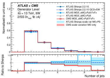
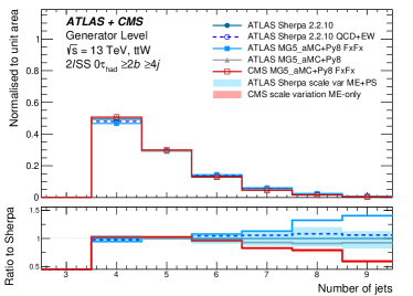
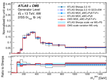
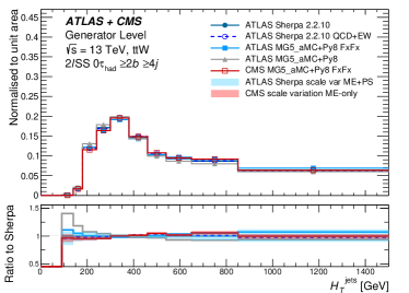
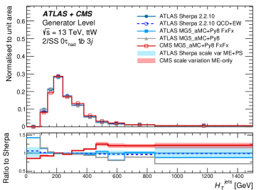
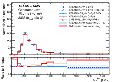
Figure 6: Distribution of the jet multiplicities (top) and the scalar sum of jets transverse momentum, $H_{\text{T}}^{\text{jets}}$ (middle), for the Region 1 with $N_{b-\text{jets}}=$1 (left) and Region 2 with $N_{b-\text{jets}}\geq$2 (right) selection requiring four and more jets, and for the Region 3 $N_{b-\text{jets}}$ = 1 (bottom, left) and Region 4 with $N_{b-\text{jets}}\geq$2 (bottom, right) selection requiring exactly three jets.

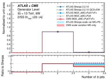
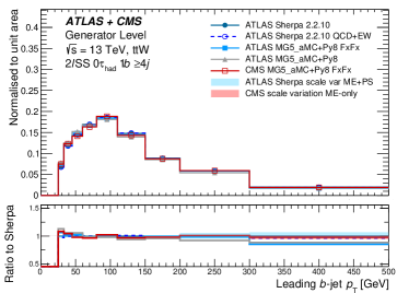
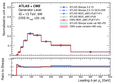
Figure 7: Distribution of the $b$-jet multiplicities (top) and the leading $b$-jet transverse momentum (bottom), for the Region 1 with $N_{b-\text{jets}}$=1 (left) and Region 2 with $N_{b-\text{jets}}\geq$2 (right) selection requiring four and more jets.

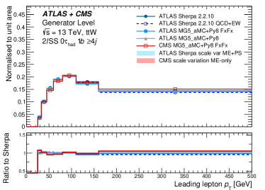
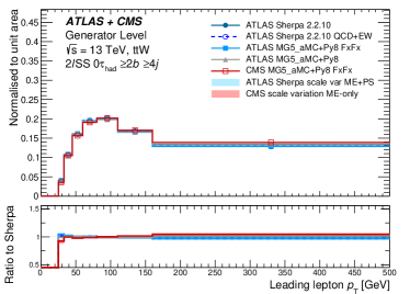
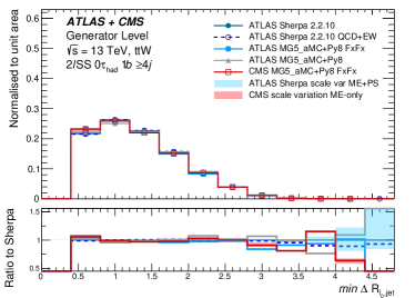
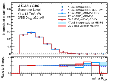
Figure 8: Distribution of the leading lepton transverse momentum (top) and the minimum angular separation between the leading lepton and the nearest jet (bottom), for the Region 1 with $N_{b-\text{jets}}$=1 (left) and Region 2 with $N_{b-\text{jets}}\geq$2 (right) selection requiring four and more jets.

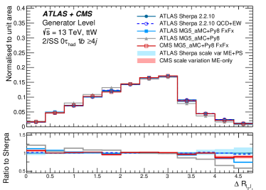
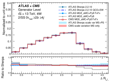
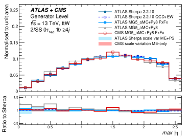
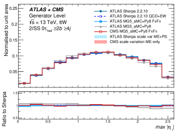
Figure 9: Distribution of the angular distance between the two leptons (top), maximum of lepton $|\eta_{\ell 0}|$ and $|\eta_{\ell 1}|$ (bottom) , for the Region 1 with $N_{b-\text{jets}}$=1 (left) and Region 2 with $N_{b-\text{jets}}\geq$2 (right) selection requiring four and more jets.

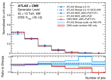
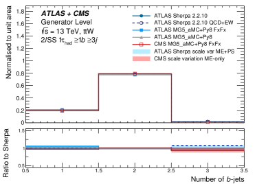
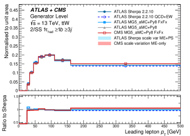
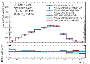
Figure 10: Distribution of the the jet multiplicity, number of $b$-jets, the leading lepton transverse momentum and the angular distance between the two leptons $\Delta R_{\ell\ell}$ for the Region 5 with 1$\tau_{\text{had}}$ selection.

3.3.2 Comparisons of predictions including acceptance effects

In the following section, a comparison of the generators will be given in the fiducial phase space, i.e. the predicted distributions include acceptance effects. For this comparison, all distributions are normalised to a common total cross section value of $\sigma_{\text{tot}}^{\text{YR4}}=$600.8\text{\,}\mathrm{fb}$$ as given in the Yellow Report 4 [47], except the distributions of Sherpa 2.2.10 QCD+EW which is normalised to its generator cross section of $614.7\text{\,}\mathrm{fb}$. The same set of distributions as discussed in Section 3.3.1 are presented. In all distributions, a significant increase of scale uncertainties is observed, reaching up to 50 % at high jet multiplicity. The observables related to jet multiplicity and $H_{\text{T}}$ show similar trends as in the shape comparisons, see Fig. 11. Only the discrepancy of the jet multiplicity prediction in MG5_aMC+Py8 FxFx is significantly enhanced.

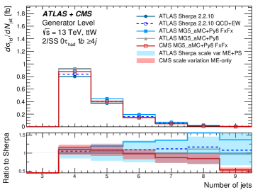
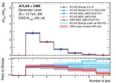
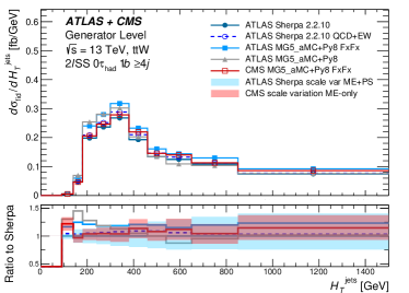
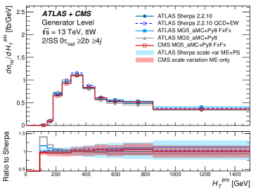
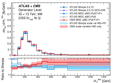
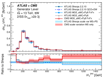
Figure 11: Distribution of jet multiplicities (top) and scalar sum of jets transverse momentum, $H_{\text{T}}^{\text{jets}}$ (middle), for the Region 1 with $N_{b-\text{jets}}$=1 (middle, left) and Region 2 with $N_{b-\text{jets}}\geq$2 (middle, right) selection requiring four and more jets. $H_{\text{T}}^{\text{jets}}$, for the Region 3 with $N_{b-\text{jets}}$=1 (bottom, left) and Region 4 with $N_{b-\text{jets}}\geq$2 (bottom, right) selection requiring exactly three jets. All distributions are normalised to the YR4 cross section of $600.8\text{\,}\mathrm{fb}$, except Sherpa 2.2.10 QCD+EW which is normalised to $614.7\text{\,}\mathrm{fb}$.

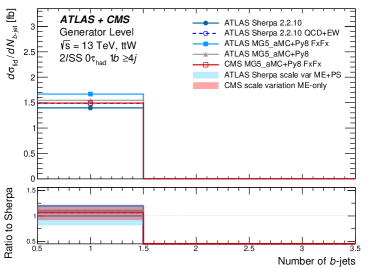
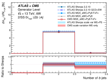
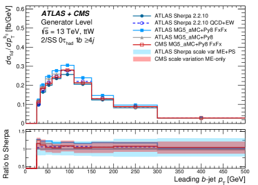
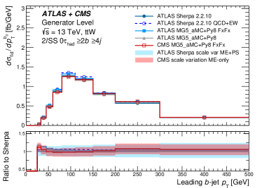
Figure 12: Distribution of the $b$-jet multiplicities (top) and the leading $b$-jet transverse momentum (bottom), for the Region 1 with $N_{b-\text{jets}}$=1 (left) and Region 2 with $N_{b-\text{jets}}\geq$2 (right) selection requiring four and more jets. All distributions are normalised to the YR4 cross section of $600.8\text{\,}\mathrm{fb}$ except Sherpa 2.2.10 QCD+EW which is normalised to $614.7\text{\,}\mathrm{fb}$.

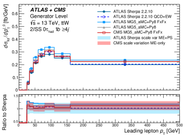
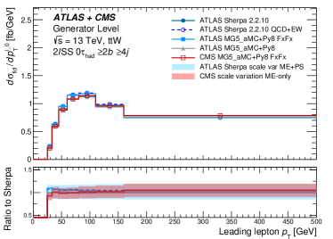
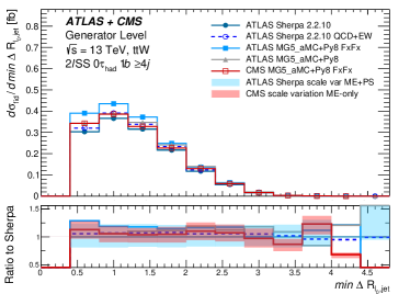
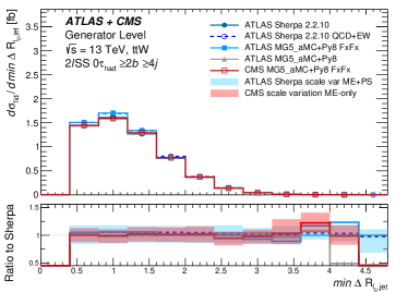
Figure 13: Distribution of the leading lepton transverse momentum (top) and the minimum angular separation between the leading lepton and the nearest jet (bottom), for the Region 1 with $N_{b-\text{jets}}$=1 (left) and Region 2 with $N_{b-\text{jets}}\geq$2 (right) selection requiring four and more jets. All distributions are normalised to the YR4 cross section of $600.8\text{\,}\mathrm{fb}$ except Sherpa 2.2.10 QCD+EW which is normalised to $614.7\text{\,}\mathrm{fb}$.

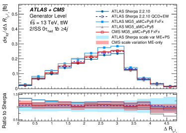
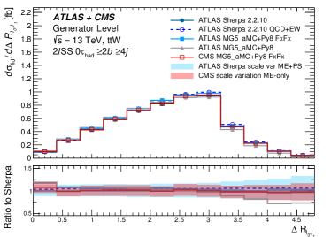
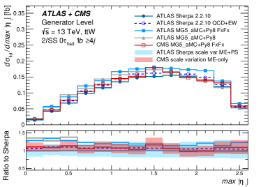
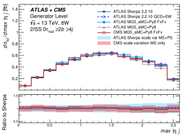
Figure 14: Distribution of the angular distance between the two leptons (top), maximum between lepton $|\eta_{\ell 0}|$ and $|\eta_{\ell 1}|$ (centre), for the Region 1 with $N_{b-\text{jets}}$=1 (left) and Region 2 with $N_{b-\text{jets}}\geq$2 (right) selection requiring four and more jets. All distributions are normalised to the YR4 cross section of $600.8\text{\,}\mathrm{fb}$ except Sherpa 2.2.10 QCD+EW which is normalised to $614.7\text{\,}\mathrm{fb}$.

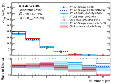
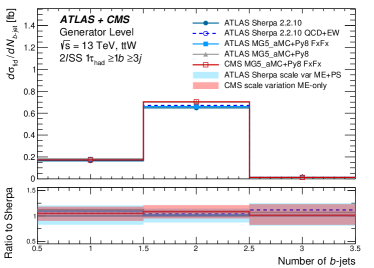
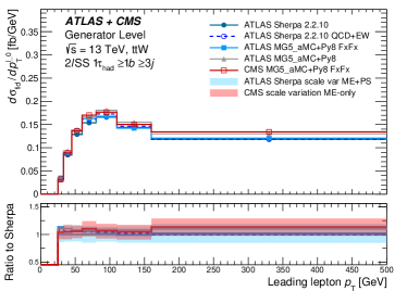
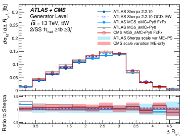
Figure 15: Distribution of the the jet multiplicity, number of $b$-jets, the leading lepton transverse momentum and the angular distance between the two leptons $\Delta R_{\ell\ell}$ for the Region 5 with 1$\tau_{\text{had}}$ selection. All distributions are normalised to the YR4 cross section of $600.8\text{\,}\mathrm{fb}$ except Sherpa 2.2.10 QCD+EW which is normalised to $614.7\text{\,}\mathrm{fb}$.

3.4 Conclusions

The $t\bar{t}W$ preditions of Sherpa and MG5_aMC@NLO+Pythia8 with different settings have been compared with respect to their inclusive ttW cross section predictions and their differential cross section predictions in regions and observables relevant for the measurement of $t\bar{t}H$ in the multi-lepton final state.

For the inclusive $t\bar{t}W$ cross section slightly different values are predicted [27, 50] for calculations with similar theoretical accuracy which is subject to ongoing theoretical studies. Based on the studies presented in this note, additional studies and discussions in the LHC Higgs Working Group and the LHC Top Working Group [73], ATLAS and CMS agreed to use the inclusive $t\bar{t}W$ cross section of $722^{+70}_{-78}$ (scale) $\pm 7$ (PDF) fb [50] as a reference inclusive cross section to allow direct comparisons between experiments.

The normalised distributions sensitive to shape differences have very small scale uncertainties, below 10 % in most of the phase space, while these scale uncertainties are significant when the acceptance effects are included, i.e. the distributions are normalised to the $t\bar{t}W$ cross section. The inclusion of tree-level EW effects only causes minor shape effects but can lead to up to 20 % difference in the cross section at high jet multiplicity. As expected, including the FxFx algorithm into the MG5_aMC@NLO+Pythia8 prediction leads to significant effects in all regions, especially at low $H_{\text{T}}$. Significant differences between the MG5_aMC@NLO+Pythia8 FxFx predictions of ATLAS and CMS are observed, especially in the jet multiplicity. Further studies are required to investigate the origin of these differences. Given that both setups consider the same perturbative accuracy such differences could be attributed to the choice of merging scale value or Pythia8 tune, so this could be an area of future study.

For many observables the shape differences between the various model predictions are within the scale uncertainties of each prediction. Observables relating to jet activity such as the jet multiplicity and $H_{\text{T}}$ are notable exceptions to this. This is especially the case for Region 3 where the differences in shape between predictions for $H_{\text{T}}$ is particlularly large. This region is important to constrain the interplay between ttW background and backgrounds arising from ttbar production where at least one lepton is mis-identified. It represents a phase space where one of the jets in the ttW decay is not reconstructed or is out of acceptance and is not expected to be as sensitive to the additional jet modelling as Regions 1 and 2. Therefore, it is somewhat surprising that such large differences are observed between predictions. This should be investigated in future studies.

The inclusion of EW corrections shows only a small shape and normalisation effects for most observables. One place where a notable effect on the shape of a distribution can be observed is for the jet multiplicity, however the effect is small enough to be covered by the QCD scale variations. Future studies could specifically target the sub-leading EW contribution with cuts related to the rapidity difference between jets which has been shown [51] to be different with respect to the central ttW QCD process.

These distributions shall be used as a starting point to derive a strategy for the theory uncertainty estimates for a combination of the expected measurement results based on the full Run-2 data set. Beyond what has been shown in the comparisons included in this document, this strategy is expected to take into consideration the latest developments on the theoretical models. For example, the NLO+PS calculations provided in Powheg [48] can act as systematic variation with respect to the MG5_aMC@NLO+Pythia8 and Sherpa calculations for more inclusive phase-spaces. They can also be used to understand parton shower, hadronisation and underlying event effects through interfaces to Pythia and Herwig. In addition, recent off-shell calculations [56, 57, 58, 59] and in particular the single-resonant contributions could be of importance. In the absence of explicit parton shower-matched calculations, corrections can be applied through the procedure outlined in Ref. [60]. It would also be important to extend existing calculations to additional final states, such as 2$\ell$SS. Finally, given the current discrepancy between ATLAS and CMS, the strategy must address how different model predictions are considered in addition to the scale uncertainties as part of the theoretical uncertainties on the measurement.

References

- [1] ATLAS Collaboration, “Measurement of Higgs boson decay into -quarks in associated production with a top-quark pair in collisions at TeV with the ATLAS detector”, arXiv:2111.06712. Submitted to JHEP (2021).
- [2] ATLAS Collaboration, “Search for the standard model Higgs boson produced in association with top quarks and decaying into a pair in collisions at with the ATLAS detector”, Phys. Rev. D 97 (2018) 072016, arXiv:1712.08895. doi:10.1103/PhysRevD.97.072016.
- [3] CMS Collaboration, “Measurement of production in the decay channel in of proton-proton collision data at ”. CMS-PAS-HIG-18-030, 2019.
- [4] CMS Collaboration, “Search for production in the H decay channel with leptonic decays in proton–proton collisions at TeV”, JHEP 03 (2019) 026, arXiv:1804.03682. doi:10.1007/JHEP03(2019)026.
- [5] ATLAS Collaboration, “Analysis of ttH and ttW production in the multilepton final states with the ATLAS detector”. ATLAS-CONF-2019-045, 2019.
- [6] CMS Collaboration, “Measurement of the Higgs boson production rate in association with top quarks in final states with electrons, muons, and hadronically decaying tau leptons at TeV”, Eur. Phys. J. C 81 (2021) 378, arXiv:2011.03652. doi:10.1140/epjc/s10052-021-09014-x.
- [7] A. Buckley, J. Butterworth, D. Grellscheid et al., “Rivet user manual”, Comput. Phys. Commun. 184 (2013) 2803–2819, arXiv:1003.0694. doi:10.1016/j.cpc.2013.05.021.
- [8] T. Sjöstrand, S. Ask, J. R. Christiansen et al., “An Introduction to PYTHIA 8.2”, Comput. Phys. Commun. 191 (2015) 159, arXiv:1410.3012. doi:10.1016/j.cpc.2015.01.024.
- [9] P. Nason, “A new method for combining NLO QCD with shower Monte Carlo algorithms”, JHEP 11 (2004) 040, arXiv:hep-ph/0409146. doi:10.1088/1126-6708/2004/11/040.
- [10] S. Frixione, P. Nason, and C. Oleari, “Matching NLO QCD computations with parton shower simulations: the POWHEG method”, JHEP 11 (2007) 070, arXiv:0709.2092. doi:10.1088/1126-6708/2007/11/070.
- [11] S. Frixione, G. Ridolfi, and P. Nason, “A positive-weight next-to-leading-order Monte Carlo for heavy flavour hadroproduction”, Journal of High Energy Physics 2007 (2007), no. 09, 126–126. doi:10.1088/1126-6708/2007/09/126.
- [12] S. Alioli, P. Nason, C. Oleari et al., “A general framework for implementing NLO calculations in shower Monte Carlo programs: the POWHEG BOX”, JHEP 06 (2010) 043, arXiv:1002.2581. doi:10.1007/JHEP06(2010)043.
- [13] J. M. Campbell, R. K. Ellis, P. Nason et al., “Top-Pair Production and Decay at NLO Matched with Parton Showers”, JHEP 04 (2015) 114, arXiv:1412.1828. doi:10.1007/JHEP04(2015)114.
- [14] A. Bredenstein, A. Denner, S. Dittmaier et al., “NLO QCD Corrections to Top Anti-Top Bottom Anti-Bottom Production at the LHC: 2. full hadronic results”, JHEP 03 (2010) 021, arXiv:1001.4006. doi:10.1007/JHEP03(2010)021.
- [15] A. Bredenstein, A. Denner, S. Dittmaier et al., “NLO QCD corrections to at the LHC”, Phys. Rev. Lett. 103 (2009) 012002, arXiv:0905.0110. doi:10.1103/PhysRevLett.103.012002.
- [16] G. Bevilacqua, M. Czakon, C. Papadopoulos et al., “Assault on the NLO wishlist:”, Journal of High Energy Physics 2009 (2009), no. 09, 109–109. doi:10.1088/1126-6708/2009/09/109.
- [17] M. V. Garzelli, A. Kardos, and Z. Trócsányi, “Hadroproduction of final states at LHC: predictions at NLO accuracy matched with Parton Shower”, JHEP 03 (2015) 083, arXiv:1408.0266. doi:10.1007/JHEP03(2015)083.
- [18] G. Bevilacqua, H.-Y. Bi, H. B. Hartanto et al., “ttbb at the LHC: on the size of corrections and b-jet definitions”, Journal of High Energy Physics 2021 (2021), no. 8,. doi:10.1007/jhep08(2021)008.
- [19] A. Denner, J.-N. Lang, and M. Pellen, “Full NLO QCD corrections to off-shell ttbb production”, Physical Review D 104 (2021), no. 5,. doi:10.1103/physrevd.104.056018.
- [20] G. Bevilacqua, H.-Y. Bi, H. B. Hartanto et al., “ at the LHC: On the size of off-shell effects and prompt -jet identification”, 2022. doi:10.48550/ARXIV.2202.11186.
- [21] T. Ježo, J. M. Lindert, N. Moretti et al., “New NLOPS predictions for -jet production at the LHC”, Eur. Phys. J. C78 (2018) 502, arXiv:1802.00426. doi:10.1140/epjc/s10052-018-5956-0.
- [22] ATLAS Collaboration, “Studies of Monte Carlo predictions for the process”. ATL-PHYS-PUB-2022-006, 2022.
- [23] J. Alwall, R. Frederix, S. Frixione et al., “The automated computation of tree-level and next-to-leading order differential cross sections, and their matching to parton shower simulations”, JHEP 07 (2014) 079, arXiv:1405.0301. doi:10.1007/JHEP07(2014)079.
- [24] R. Frederix and S. Frixione, “Merging meets matching in MC@NLO”, JHEP 12 (2012) 061, arXiv:1209.6215. doi:10.1007/JHEP12(2012)061.
- [25] J. Bellm, S. Gieseke, D. Grellscheid et al., “Herwig 7.0/Herwig++ 3.0 release note”, The European Physical Journal C 76 (2016), no. 4,. doi:10.1140/epjc/s10052-016-4018-8.
- [26] B. Cooper, J. Katzy, M. L. Mangano et al., “Importance of a consistent choice of alpha(s) in the matching of AlpGen and Pythia”, Eur. Phys. J. C 72 (2012) 2078, arXiv:1109.5295. doi:10.1140/epjc/s10052-012-2078-y.
- [27] Sherpa Collaboration, “Event Generation with Sherpa 2.2”, SciPost Phys. 7 (2019) 034, arXiv:1905.09127. doi:10.21468/SciPostPhys.7.3.034.
- [28] F. Cascioli, P. Maierhöfer, N. Moretti et al., “NLO matching for production with massive -quarks”, Phys. Lett. B734 (2014) 210–214, arXiv:1309.5912. doi:10.1016/j.physletb.2014.05.040.
- [29] F. Cascioli, P. Maierhofer, and S. Pozzorini, “Scattering Amplitudes with Open Loops”, Phys. Rev. Lett. 108 (2012) 111601, arXiv:1111.5206. doi:10.1103/PhysRevLett.108.111601.
- [30] The routine will be released as MC-ttbb routine in the Rivet analysis toolkit [7].
- [31] A. Ryd, D. Lange, N. Kuznetsova et al., “EvtGen: A Monte Carlo Generator for B-Physics”. EVTGEN-V00-11-07, 2005.
- [32] F. Buccioni, S. Kallweit, S. Pozzorini et al., “NLO QCD predictions for production in association with a light jet at the LHC”, JHEP 12 (2019) 015, arXiv:1907.13624. doi:10.1007/JHEP12(2019)015.
- [33] ATLAS Collaboration, “ATLAS Pythia 8 tunes to data”. ATL-PHYS-PUB-2014-021, 2014.
- [34] CMS Collaboration, “Extraction and validation of a new set of CMS Pythia tunes from underlying-event measurements”, Eur. Phys. J. C 80 (2020) 4, arXiv:1903.12179. doi:10.1140/epjc/s10052-019-7499-4.
- [35] T. Gleisberg and S. Höche, “Comix, a new matrix element generator”, JHEP 12 (2008) 039, arXiv:0808.3674. doi:10.1088/1126-6708/2008/12/039.
- [36] S. Schumann and F. Krauss, “A Parton shower algorithm based on Catani-Seymour dipole factorisation”, JHEP 03 (2008) 038, arXiv:0709.1027. doi:10.1088/1126-6708/2008/03/038.
- [37] T. Ježo and P. Nason, “On the Treatment of Resonances in Next-to-Leading Order Calculations Matched to a Parton Shower”, JHEP 12 (2015) 065, arXiv:1509.09071. doi:10.1007/JHEP12(2015)065.
- [38] M. Cacciari, G. P. Salam, and G. Soyez, “The anti- jet clustering algorithm”, JHEP 04 (2008) 063, arXiv:0802.1189. doi:10.1088/1126-6708/2008/04/063.
- [39] M. Cacciari, G. P. Salam, and G. Soyez, “FastJet user manual”, Eur. Phys. J. C 72 (2012) 1896, arXiv:1111.6097. doi:10.1140/epjc/s10052-012-1896-2.
- [40] M. Cacciari, G. P. Salam, and G. Soyez, “The Catchment Area of Jets”, JHEP 04 (2008) 005, arXiv:0802.1188. doi:10.1088/1126-6708/2008/04/005.
- [41] CMS Collaboration, “Measurement of the cross section of top quark-antiquark pair production in association with a W boson in proton-proton collisions at ”. CMS-PAS-TOP-21-011, 2022.
- [42] F. Maltoni, M. L. Mangano, I. Tsinikos et al., “Top-quark charge asymmetry and polarization in production at the LHC”, Phys. Lett. B 736 (2014) 252–260, arXiv:1406.3262. doi:10.1016/j.physletb.2014.07.033.
- [43] J. M. Campbell and R. K. Ellis, “ production and decay at NLO”, JHEP 07 (2012) 052, arXiv:1204.5678. doi:10.1007/JHEP07(2012)052.
- [44] M. V. Garzelli, A. Kardos, C. G. Papadopoulos et al., “t and t Z Hadroproduction at NLO accuracy in QCD with Parton Shower and Hadronization effects”, JHEP 11 (2012) 056, arXiv:1208.2665. doi:10.1007/JHEP11(2012)056.
- [45] F. Maltoni, D. Pagani, and I. Tsinikos, “Associated production of a top-quark pair with vector bosons at NLO in QCD: impact on searches at the LHC”, JHEP 02 (2016) 113, arXiv:1507.05640. doi:10.1007/JHEP02(2016)113.
- [46] S. Frixione, V. Hirschi, D. Pagani et al., “Electroweak and QCD corrections to top-pair hadroproduction in association with heavy bosons”, JHEP 06 (2015) 184, arXiv:1504.03446. doi:10.1007/JHEP06(2015)184.
- [47] D. de Florian et al., “Handbook of LHC Higgs Cross Sections: 4. Deciphering the Nature of the Higgs Sector”, arXiv:1610.07922. (2017). doi:10.23731/CYRM-2017-002.
- [48] F. Febres Cordero, M. Kraus, and L. Reina, “Top-quark pair production in association with a gauge boson in the POWHEG-BOX”, Phys. Rev. D 103 (2021), no. 9, 094014, arXiv:2101.11808. doi:10.1103/PhysRevD.103.094014.
- [49] S. von Buddenbrock, R. Ruiz, and B. Mellado, “Anatomy of inclusive production at hadron colliders”, Phys. Lett. B 811 (2020) 135964, arXiv:2009.00032. doi:10.1016/j.physletb.2020.135964.
- [50] R. Frederix and I. Tsinikos, “On improving NLO merging for production”, JHEP 11 (2021) 029, arXiv:2108.07826. doi:10.1007/JHEP11(2021)029.
- [51] J. A. Dror, M. Farina, E. Salvioni et al., “Strong tW Scattering at the LHC”, JHEP 01 (2016) 071, arXiv:1511.03674. doi:10.1007/JHEP01(2016)071.
- [52] R. Frederix, D. Pagani, and M. Zaro, “Large NLO corrections in and hadroproduction from supposedly subleading EW contributions”, JHEP 02 (2018) 031, arXiv:1711.02116. doi:10.1007/JHEP02(2018)031.
- [53] A. Kulesza, L. Motyka, D. Schwartländer et al., “Associated production of a top quark pair with a heavy electroweak gauge boson at NLONNLL accuracy”, Eur. Phys. J. C 79 (2019), no. 3, 249, arXiv:1812.08622. doi:10.1140/epjc/s10052-019-6746-z.
- [54] A. Broggio, A. Ferroglia, R. Frederix et al., “Top-quark pair hadroproduction in association with a heavy boson at NLO+NNLL including EW corrections”, JHEP 08 (2019) 039, arXiv:1907.04343. doi:10.1007/JHEP08(2019)039.
- [55] A. Kulesza, L. Motyka, D. Schwartländer et al., “Associated top quark pair production with a heavy boson: differential cross sections at NLO+NNLL accuracy”, Eur. Phys. J. C 80 (2020), no. 5, 428, arXiv:2001.03031. doi:10.1140/epjc/s10052-020-7987-6.
- [56] G. Bevilacqua, H.-Y. Bi, H. B. Hartanto et al., “The simplest of them all: at NLO accuracy in QCD”, JHEP 08 (2020) 043, arXiv:2005.09427. doi:10.1007/JHEP08(2020)043.
- [57] A. Denner and G. Pelliccioli, “NLO QCD corrections to off-shell production at the LHC”, JHEP 11 (2020) 069, arXiv:2007.12089. doi:10.1007/JHEP11(2020)069.
- [58] G. Bevilacqua, H.-Y. Bi, H. B. Hartanto et al., “NLO QCD corrections to off-shell production at the LHC: correlations and asymmetries”, Eur. Phys. J. C 81 (2021), no. 7, 675, arXiv:2012.01363. doi:10.1140/epjc/s10052-021-09478-x.
- [59] A. Denner and G. Pelliccioli, “Combined NLO EW and QCD corrections to off-shell production at the LHC”, Eur. Phys. J. C 81 (2021), no. 4, 354, arXiv:2102.03246. doi:10.1140/epjc/s10052-021-09143-3.
- [60] G. Bevilacqua, H. Y. Bi, F. Febres Cordero et al., “Modeling uncertainties of multilepton signatures”, Phys. Rev. D 105 (2022), no. 1, 014018, arXiv:2109.15181. doi:10.1103/PhysRevD.105.014018.
- [61] T. Gleisberg, S. Höche, F. Krauss et al., “Event generation with SHERPA 1.1”, JHEP 02 (2009) 007, arXiv:0811.4622. doi:10.1088/1126-6708/2009/02/007.
- [62] S. Höche, F. Krauss, M. Schönherr et al., “QCD matrix elements + parton showers: The NLO case”, JHEP 04 (2013) 027, arXiv:1207.5030. doi:10.1007/JHEP04(2013)027.
- [63] S. Kallweit, J. M. Lindert, P. Maierhofer et al., “NLO QCD+EW predictions for V + jets including off-shell vector-boson decays and multijet merging”, JHEP 04 (2016) 021, arXiv:1511.08692. doi:10.1007/JHEP04(2016)021.
- [64] C. Gütschow, J. M. Lindert, and M. Schönherr, “Multi-jet merged top-pair production including electroweak corrections”, Eur. Phys. J. C 78 (2018), no. 4, 317, arXiv:1803.00950. doi:10.1140/epjc/s10052-018-5804-2.
- [65] ATLAS Collaboration, “Modelling of rare top quark processes at TeV”. ATL-PHYS-PUB-2020-024, 2020.
- [66] P. Artoisenet, R. Frederix, O. Mattelaer et al., “Automatic spin-entangled decays of heavy resonances in Monte Carlo simulations”, JHEP 03 (2013) 015, arXiv:1212.3460. doi:10.1007/JHEP03(2013)015.
- [67] S. Catani, F. Krauss, R. Kuhn et al., “QCD matrix elements + parton showers”, JHEP 11 (2001) 063, arXiv:hep-ph/0109231. doi:10.1088/1126-6708/2001/11/063.
- [68] K. Hamilton, P. Nason, and G. Zanderighi, “MINLO: Multi-Scale Improved NLO”, JHEP 10 (2012) 155, arXiv:1206.3572. doi:10.1007/JHEP10(2012)155.
- [69] J. Alwall et al., “A Standard format for Les Houches event files”, Comput. Phys. Commun. 176 (2007) 300–304, arXiv:hep-ph/0609017. doi:10.1016/j.cpc.2006.11.010.
- [70] J. Alwall, R. Frederix, S. Frixione et al., “The automated computation of tree-level and next-to-leading order differential cross sections, and their matching to parton shower simulations”, Journal of High Energy Physics 2014 (2014). doi:10.1007/jhep07(2014)079.
- [71] NNPDF Collaboration, “Parton distributions for the LHC Run II”, JHEP 04 (2015) 040, arXiv:1410.8849. doi:10.1007/JHEP04(2015)040.
- [72] NNPDF Collaboration, “Parton distributions from high-precision collider data”, Eur. Phys. J. C 77 (2017), no. 10, 663, arXiv:1706.00428. doi:10.1140/epjc/s10052-017-5199-5.
- [73] LHC Higgs and Top Working Groups, “ttW modeling in light of ttH measurements”, 2022. https://indico.cern.ch/event/1219500/.