Predator Extinction arose from Chaos of the Prey: the Chaotic Behavior of a Homomorphic Two-Dimensional Logistic Map in the Form of Lotka-Volterra Equations

Abstract

A two-dimensional homomorphic logistic map that preserves features of Lotka-Volterra Equations was proposed. In order to examine the Lotka-Volterra chaos, in addition to ordinary iteration plots of population, Lyapunov exponents either calculated directly from eigenvalues of Jacobian of the $2$D logistic mapping, or from time-series algorithms of both Rosenstein and Eckmann et al. were calculated, among which discrepancies were compared. Bifurcation diagrams may be divided into five categories depending on different topological shapes, among which flip bifurcation and Neimark-Sacker bifurcation were observed, the latter showing closed orbits around limit circles in the phase portrait and phase space diagram. Our model restored the $1$D logistic map of the prey at the absence of the predator, as well as the normal competing behavior between two species when the initial population of the two is equal. In spite of the possibility for two species going into chaos simultaneously, it is also possible that with the same inter-species parameters as normal but with predator population $10$ times more than that of the prey, under certain growth rate the latter becomes chaotic, and former dramatically reduces to zero, referring to total annihilation of the predator species. Interpreting humans as the predator and natural resources as the prey in the ecological system, the aforementioned conclusion may imply that not only excessive consumption of the natural resources, but its chaotic state triggered by overpopulation of humans may also backfire in a manner of total extinction on human species. Fortunately, a little chance may exist for survival of human race, as isolated fixed points in bifurcation diagram of the predator reveals.

Keywords Chaos, Neimark-Sacker Bifurcation, Logistic Map, Lyapunov Exponents, Lotka-Volterra Equations, Extinction of Species

1 Introduction

Understanding interactions between human beings and natural resources plays an important role in establishing sustainable economy and society. Relationships of these two may be studied by the prey and predator model after we realize that humans beings may be regarded as the predator while natural resources may be thought of as the prey[1]. Afterwards, researches on the prey-predator models may be implemented to this field instinctively[2]-[3].

Generally speaking, there are two main approaches of studies in the literature to this prey and predator model. The first is to study differential equations, while the other is to study the iterations in difference equations, whose forms may be inspired by directly applying the forward Euler’s Scheme to acquire counterpart of the former[4]-[10]. The discrete model could be more promising than the continuous one, because it has more abundant dynamic characteristics in chaotic behaviors[8], whereas it would be more difficult for solutions to continuous models to reach chaos in low dimensional cases. Taking some examples about the first approach, studies[11]-[12] have performed on chaos of Lotka-Volterra differential equations with dimensions higher than three, and researchers[13] claimed that it is impossible to reach chaos for two species in the form of differential Lotka-Volterra Equations, whose general solutions were obtained in sinusoidal forms by Evans and Findley[14]. Additionally, based on the Lotka-Volterra model, Dunbar[15] confirmed the existence of traveling wave solutions for two reaction diffusion systems. Besides that, Das and Gupta[16] proposed solutions to the fractional-order time derivative Lotka-Volterra equations using an analytical approach for nonlinear problems known as the homotopy perturbation method (HPM).

On the other hand, there are also several studies on the discrete difference equations. For instance, Bessoir and Wolf [17] made pioneering contributions to the application of $1$D logistic equation on biological and ecological studies. The same equation was also used to interpret, analyze and predict data according to the COVID-19 by many researchers[18]. Mareno and English[19] implemented the $1$D logistic equation to the coupled $2$D logistic one, and demonstrated that for large growth rate the system underwent a Neimark-Sacker bifurcation. Li et al.[20] imposed an equal individual effect intensity, corresponding to equal growth rate in the $1$D logistic map, on the two oligopolists in the homomorphic Kopel model and observed three different kinds of bifurcation. Furthermore, Elhadi and Sprott[21] proposed a two-dimensional mapping, one of which is the ordinary $1$D logistic map while the other consists of a perturbation term of the former and is also modulated by the first. Shilnikov and Rulkov[22] studied chaos behaviors in two-dimensional difference equations that reproduced spike-bursting activities in biological neurons, improving further on the previous research based on the three-dimensional system of ODEs. In spite of applying the forward Euler’s Scheme to acquire the difference equation, researchers also made use of exponential forms corresponding to solutions on the differential equations. For example, Ishaque et al.[23] studied a three dimensional predator-prey-parasite model with an exponential form describing interactions among healthy or infected Tilapia fish as the prey, and Pelican birds as the predator. Tassaddiq et al.[24] worked on discrete-time exponential difference equation of Leslie-Gower predator-prey model together with a Holling type III functional response, and indicated the advantage on this type of discretization method. Previous study[25] suggested a heteromorphic term describing the decreasing effects on the predator that was only linear to the population of that species, contrary to the corresponding quadratic term in the prey. Hassell et al[26] applied the predator-prey model to insect parasitoids and anthropods, and found out that local movements of the two species may cause extermination of the entire ecological system with chaos, and it is difficult to maintain population stability for large growth rate of anthropods. Besides, researchers[27] also pointed out that human misbehavior may be the reason for an ecological system to go into chaotic states.

However, there is no convincing reason for the prey and the predator to have different forms in the difference equations. Intuition in mathematical symmetry naturally came to our mind that a successful predator-prey difference model should resemble the symmetry structure as in Lotka-Volterra differential equations. Moreover, solutions to Lotka-Volterra Equations in sinusoidal forms cannot explain extinction of species.

We proposed homomorphic two-dimensional logistic maps that preserve both forms of Lotka-Volterra Equations and the $1$D logistic equation. In our model, we conjectured a quadractic form in both corresponding terms of the prey and the predator, treating both species on the equal stance. Structures of Bifurcation diagrams showed that there could be six different categories in our dynamic system. For each categories, we examined population iterations, phase portraits, phase space diagrams, and topological types of fixed points. Lyapunov exponents either calcaulted from eigenvalues of Jacobian of the $2$D mapping or from time-series algorithms either Rosenstein[28] or Eckmann et al.[29] were also calculated. Comparisons among those results were also discussed.

The advantages of our model include the following. First, we may be able to establish a standard bifurcation diagram of $1$D logistic map about the prey with nonzero initial predator population, growth rates in both species, and predation parameters. Second, our model may also describe the normal behavior of rise and fall on the population of the two species when interacting with each other. Third, besides simultaneous chaos in both species, the main discovery in our research was that the predator may go extinct under the circumstance of chaos in the prey that the predator overpopulation should be blamed.

2 Theorems

We first review the one-dimensional logistic equation and the two-dimensional Lotka-Volterra Equations, comparing the similarity and difference between the two sets of equations, which inspires us on the idea to establish two-dimensional logistic equations that maintain important features about both of the above equations.

2.1 Review on the $1$D logistic equation and Litka-Volterra Equations

To begin with, the one-dimensional logistic equation may be written as

$$x_{n+1}=\mu_{0}x_{n}(1-x_{n}),$$ (1)

where $\mu_{0}$ denotes to the growth rate.

On the other hand, the two-dimensional Lotka-Volterra Equations$\cite[cite]{[\@@bibref{}{Lotka}{}{}]},\cite[cite]{[\@@bibref{}{Volterra}{}{}]}$ describe interactions between the prey and predator in an environment where there is sufficient food supply for the prey, whose only natural enemy is the predator. The formula may be written as follows:

$$\frac{dx}{dt} =\mu_{0}x-\mu_{1}xy;$$ (2a)

$$\frac{dy}{dt} =-\nu_{0}y+\nu_{1}xy,$$ (2b)

where $\mu_{0}$, $\mu_{1}$, $\nu_{0}$, and $\nu_{1}$ are all positive inter-species parameters. $x$ denotes population of the prey while $y$, population of the predator, both being positive real numbers. $\mu_{0}$ and $\nu_{1}$ are, respectively, growth rate of the prey and the predator. While $\mu_{1}$ refers to the parameter for predation to occur upon the prey at the presence of predator, $\nu_{0}$ refers to all effects that decrease population of the predator, which may include disease, death, or emigration[32]. With forward Euler’s scheme, one may immediately write the difference version of Eq.(2) as follows

$$x_{n+1}-x_{n} =\mu_{0}x_{n}-\mu_{1}x_{n}y_{n};$$ (3a)

$$y_{n+1}-y_{n} =-\nu_{0}y_{n}+\nu_{1}x_{n}y_{n}.$$ (3b)

However, there is an obvious drawback about the above simultaneous equations: it does not preserve the feature of $1$D logistic equation, because the first term on the right hand side is either linear to $x_{n}$ or $y_{n}$, whereas the right hand side in Eq.(1) is quadratic to $x_{n}$.

We now discuss our idea on establishing the two-dimensional map that resembles interaction terms of the prey and the predator as in Lotka-Volterra. First, we may rewrite the linear term of $x$ on the right hand side of Eq.(2a) into quadratic, which looks like $\mu_{0}x(1-x)$, together with the homomorphic corresponding term in Eq.(2b) as $\nu_{0}y(1-y)$. Thus, the modified Lotka-Volterra Equations[33] are

$$\frac{dx}{dt} =\mu_{0}x(1-x)-\mu_{1}xy;$$ (4a)

$$\frac{dy}{dt} =-\nu_{0}y(1-y)+\nu_{1}xy,$$ (4b)

whose resemblance in the form of difference equations are, therefore,

$$x_{n+1}-x_{n} =\mu_{0}x_{n}(1-x_{n})-\mu_{1}x_{n}y_{n};$$ (5a)

$$y_{n+1}-y_{n} =-\nu_{0}y_{n}(1-y_{n})+\nu_{1}x_{n}y_{n}.$$ (5b)

Even though it seems more reasonable to direct resemblance of Lotka-Volterra Equations, Eq.(5) fails to restore Eq.(1) when parameters other than $\mu_{0}$ are all set to be zero. Fortunately, we may modify this by dropping $x_{n}$ and $y_{n}$ terms on the left hand side of the above equations

$$x_{n+1} =\mu_{0}x_{n}(1-x_{n})-\mu_{1}x_{n}y_{n};$$ (6a)

$$y_{n+1} =-\nu_{0}y_{n}(1-y_{n})+\nu_{1}x_{n}y_{n},$$ (6b)

which is the desired form. We divided into two cases to study further about properties of Eq.(5) and Eq.(6) in Sec. 2.3 and Sec. 2.4. But before that, in next subsection we first discuss a very important lemma that allows us to study stability behaviors of fixed points.

2.2 Stability of fixed points

Suppose a mapping of two-dimensional iterations $x_{n+1}$ and $y_{n+1}$ are written as $x_{n+1}=f(x,y)$ and $y_{n+1}=g(x,y)$. The Jacobian is, therefore,

$$J =\frac{\partial(f,g)}{\partial(x,y)}$$ (7a)

$$=\begin{pmatrix}\frac{\partial f}{\partial x}&\frac{\partial f}{\partial y}\\ \frac{\partial g}{\partial x}&\frac{\partial g}{\partial y}\end{pmatrix},$$ (7b)

whose eigenvalus are $\omega_{0}$ and $\omega_{1}$. It is well known[6], [8] that a fixed point may be divided into the following four topological types based on their stability behaviors. First, it could be a sink and locally asymptotic stable if eigenvalues of Eq.(7) satisfy $|\omega_{0}|<1$ and $|\omega_{1}|<1$. Second, it could be a source and locally unstable if eigenvalues satisfy $|\omega_{0}|>1$ and $|\omega_{1}|>1$. Third, a fixed point could be a saddle if one of the absolute values of the eigenvalues is greater than $1$ while the other is smaller than $1$. At last, a fixed point could be non-hyperbolic if one of the absolute values of the eigenvalues is equal to $1$. The stability of a non-hyperbolic fixed point is fragile[34], which means that its stability is easily influenced by the small nonlinear terms.

Instead of calculating the range of eigenvalues directly, most of the time it is more convenient to work with the quadratic formula consisting of eigenvalues $\omega_{0}$ and $\omega_{1}$, namely, $\Omega(\omega)=\omega^{2}-\mathrm{Tr(J)}\omega+\mathrm{det(J)},$ where $\mathrm{Tr(J)}$ and $\mathrm{det(J)}$ are trace and determinant of Jacobian in Eq.(7), respectively, and there could be a correspondence on the stability behavior around a fixed point between the roots of the quadratic formual, $\omega_{0}$ and $\omega_{1}$, which are also eigenvalues of Jacobian, through the following Lemma

Lemma 1.

Let $\Omega(\omega)=\omega^{2}-\mathrm{Tr(J)}\omega+\mathrm{det(J)},$ be a quadratic formula where where $\mathrm{Tr(J)}$ and $\mathrm{det(J)}$ are trace and determinant of Jacobian in Eq.$\mathrm{(\ref{eq:Jacobian general case})}$, respectively. Then

1. If $\Omega(1)>0$, then

   1. $|\omega_{0}|<1$ and $|\omega_{1}|<1$ and hence the fixed point is a sink if and only if $\Omega(-1)>0$ and $\mathrm{det(J)}<1$;

   2. $|\omega_{0}|>1$ and $|\omega_{1}|>1$ and hence the fixed point is a source if and only if $\Omega(-1)>0$ and $\mathrm{det(J)}>1$;

   3. One of $|\omega_{0}|$ and $|\omega_{1}|$ is smaller than $1$ while the other greater than $1$ and hence the fixed point is a saddle if and only if $\Omega(-1)<0$;

   4. Either $|\omega_{0}|$ or $|\omega_{1}|$ is equal to $1$ and hence the fixed point is a non-hyperbolic whenever

      1. $\omega_{0}=-1$ and $\omega_{1}\neq-1$ if and only if $\Omega(-1)=0$ and $\mathrm{Tr(J)}\neq 2$.

      2. $\omega_{0}$ and $\omega_{1}$ are a pair of complex conjugates and $|\omega_{0}|=|\omega_{1}|=1$ if and only if $|\mathrm{Tr(J)}|<2$ and $\mathrm{det(J)}=1$.

      3. $\omega_{0}=\omega_{1}=-1$ if and only if $\Omega(-1)=0$ and $\mathrm{Tr(J)}=2$.

2. If $\Omega(1)=0$, then either $|\omega_{0}|$ or $|\omega_{1}|$ has to be equal to $1$. Therefore the fixed point is a non-hyperbolic. Absolute value of the other root is greater than, equal to, or smaller than $1$ if and only if, correspondingly, absolute value of $\mathrm{det(J)}$ is greater than, equal to, or smaller than $1$.

3. If $\Omega(1)<0$, then either $|\omega_{0}|$ or $|\omega_{1}|$ has to be real and greater than $1$. Therefore, the fixed point is a saddle. Further,

   1. the other root is smaller or equal to $-1$ if and only if, correspondingly, $\Omega(-1)<-1$ or $\Omega(-1)=-1$.

   2. absolute value of the other root is smaller than $1$ if and only if $\Omega(-1)>0$.

1 makes it easier for us to study analytically the stability of fixed points.

2.3 Properties of Eq.(5)

Setting up $x_{n+1}=f(x,y)$ and $y_{n+1}=g(x,y)$, the two-dimensional logistic equations in Eq.(5) have the mappings

$$f(x,y) =\mu_{0}x(1-x)-\mu_{1}xy+x;$$ (8a)

$$g(x,y) =-\nu_{0}y(1-y)+\nu_{1}xy+y.$$ (8b)

Eq.(8) has Jacobian, as indicated in Eq.(7),

$$J=\begin{pmatrix}\mu_{0}(1-2x)-\mu_{1}y+1&-\mu_{1}x\\ \nu_{1}y&\nu_{0}(-1+2y)+\nu_{1}x+1\end{pmatrix},$$ (9)

with eigenvalues $\omega_{0}$ and $\omega_{1}$ being, respectively,

$$\omega_{0} =-\mu_{0}x+\nu_{0}y+1+\frac{1}{2}(x\nu_{1}-y\mu_{1})+\frac{1}{2}(\mu_{0}-\nu_{0})+\frac{\omega}{2}$$ (10a)

$$\omega_{1} =-\mu_{0}x+\nu_{0}y+1+\frac{1}{2}(x\nu_{1}-y\mu_{1})+\frac{1}{2}(\mu_{0}-\nu_{0})-\frac{\omega}{2}$$ (10b)

where

$$\omega =\Bigg{[}4(\nu_{0}+\frac{\mu_{1}}{2})^{2}y^{2}+\Bigg{(}\bigg{(}(4\mu_{0}-2\nu_{1})\mu_{1}+8\nu_{0}(\mu_{0}+\frac{\nu_{1}}{2})\bigg{)}x-4(\nu_{0}+\mu_{0})(\nu_{0}+\frac{\mu_{1}}{2})\Bigg{)}y$$ (11)

$$+4\bigg{(}(\mu_{0}+\frac{\nu_{1}}{2})x-\frac{\mu_{0}}{2}-\frac{\nu_{0}}{2}\bigg{)}^{2}\Bigg{]}^{\frac{1}{2}}$$

Further, fixed points, at which pairs of $x$ and $y$ stay still irrespective of time-series iterations[34], are those pairs of points $(x^{*},y^{*})$ such that

$$x^{*} =\mu_{0}x^{*}(1-x^{*})-\mu_{1}x^{*}y^{*}+x^{*}$$ (12a)

$$y^{*} =\nu_{0}y^{*}(1-y^{*})-\nu_{1}x^{*}y^{*}+y^{*},$$ (12b)

from which four pairs of fixed points $(x^{*},y^{*})$ may be derived as

$$E_{0}=(0,0)$$ (13a)

$$E_{1}=(0,1)$$ (13b)

$$E_{2}=(1,0)$$ (13c)

$$E_{3}=\bigg{(}\frac{\nu_{0}(\mu_{1}-\mu_{0})}{-\mu_{0}\nu_{0}+\mu_{1}\nu_{1}},\frac{\mu_{0}(\nu_{1}-\nu_{0})}{-\mu_{0}\nu_{0}+\mu_{1}\nu_{1}}\bigg{)},$$ (13d)

provided that the denominator in Eq.(13d) is not zero. On the contrary, however, when $\mu_{0}\nu_{0}=\mu_{1}\nu_{1}$, Eq.(5) has fixed points $E_{0}$, $E_{1}$,and $E_{2}$.

Keeping Lamma 1 in Sec. 2.2 in mind, we may be able to examine the topological type of each fixed point in Eq.(13) as in Theorem 1:

Theorem 1.

The topological types of fixed points in Eq.(13) are

1. For $E_{0}=(0,0)$,

   $$\Omega(1) =-\mu_{0}\nu_{0}$$

   $$\Omega(-1) =(2+\mu_{0})(2-\nu_{0})$$

   $$\mathrm{det(J)} =(1+\mu_{0})(1-\nu_{0})$$

   $$\mathrm{Tr(J)} =2+\mu_{0}-\nu_{0}.$$

   Because $\Omega(1)<0$, therefore, $E_{0}$ is always a saddle.

2. For $E_{1}=(0,1)$,

   $$\Omega(1) =\nu_{0}(\mu_{0}-\mu_{1})$$

   $$\Omega(-1) =(2+\nu_{0})(2+\mu_{0}-\mu_{1})$$

   $$\mathrm{det(J)} =(1+\nu_{0})(1+\mu_{0}-\mu_{1})$$

   $$\mathrm{Tr(J)} =2+\mu_{0}-\mu_{1}+\nu_{0}.$$

   In this case,

   1. $E_{1}$ cannot be a sink;

   2. if $\mu_{0}>\mu_{1}$, then $E_{1}$ is a source;

   3. if $\mu_{0}<\mu_{1}$, then $E_{1}$ is a saddle.

   4. if $\mu_{0}=\mu_{1}$, then $E_{1}$ is a non-hyperbole;

3. For $E_{2}=(1,0)$,

   $$\Omega(1) =-\mu_{0}(\nu_{1}-\nu_{0})$$

   $$\Omega(-1) =(2-\mu_{0})(2+\nu_{1}-\nu_{0})$$

   $$\mathrm{det(J)} =(1-\mu_{0})(1+\nu_{1}-\nu_{0})$$

   $$\mathrm{Tr(J)} =2-\mu_{0}+(\nu_{1}-\nu_{0}).$$

   In this case,

   1. if $\mu_{0}<2$ and $\nu_{1}<\nu_{0}<\nu_{1}+1$ and $\nu_{1}<\nu_{0}$, or $\mu_{0}<2$ and $\nu_{0}=\nu_{1}+1$, or $\mu_{0}<2$ and $\nu_{1}+1<\nu_{0}<\nu_{1}+2$, then $E_{2}$ is a sink;

   2. if $\mu_{0}>2$ and $\nu_{0}>\nu_{1}+2$, then $E_{2}$ is a source;

   3. if $\mu_{0}>2$ and $\nu_{1}<\nu_{0}<\nu_{1}+2$, or $\mu_{0}<2$ and $\nu_{0}>\nu_{1}+2$, or $\nu_{1}>\nu_{0}$, then $E_{2}$ is a saddle;

   4. if $\nu_{1}=\nu_{0}$, then $E_{2}$ is a non-hyperbole.

4. For $E_{3}=\bigg{(}\frac{\nu_{0}(\mu_{1}-\mu_{0})}{-\mu_{0}\nu_{0}+\mu_{1}\nu_{1}},\frac{\mu_{0}(\nu_{1}-\nu_{0})}{-\mu_{0}\nu_{0}+\mu_{1}\nu_{1}}\bigg{)}$,

   $$\Omega(1) =-\frac{\mu_{0}\nu_{0}(\nu_{0}-\nu_{1})(\mu_{0}-\mu_{1})}{\mu_{0}\nu_{0}-\mu_{1}\nu_{1}}$$

   $$\Omega(-1) =\frac{-\nu_{0}(\nu_{0}-\nu_{1}+2)\mu_{0}^{2}+\nu_{0}(\mu_{1}+2)(\nu_{0}-\nu_{1}+2)\mu_{0}-4\mu_{1}\nu_{1}}{\mu_{0}\nu_{0}-\mu_{1}\nu_{1}}$$

   $$\mathrm{det(J)} =\frac{-\nu_{0}(\nu_{0}-\nu_{1}+1)\mu_{0}^{2}+\nu_{0}(\mu_{1}+1)(\nu_{0}-\nu_{1}+1)\mu_{0}-\mu_{1}\nu_{1}}{\mu_{0}\nu_{0}-\mu_{1}\nu_{1}}$$

   $$\mathrm{Tr(J)} =\frac{-\mu_{0}^{2}\nu_{0}+\nu_{0}(\nu_{0}+\mu_{1}-\nu_{1}+2)\mu_{0}-2\mu_{1}\nu_{1}}{\mu_{0}\nu_{0}-\mu_{1}\nu_{1}}.$$

   In this case,

   1. if $\mu_{0}<\mu_{1}$ and $\mu_{0}^{2}\nu_{0}<\mu_{1}^{2}\nu_{1}$, or $\mu_{0}>\mu_{1}$ and $\mu_{0}^{2}\nu_{0}>\mu_{1}^{2}\nu_{1}$, then it is a saddle;

   2. if $\mu_{0}^{2}/\mu_{1}^{2}=\nu_{1}/\nu_{0}$, we have a non-hyperbole in the interior region.

In order to plot bifurcation diagrams, we further assume that $\mu_{1}=\alpha\mu_{0}$, $\nu_{0}=\beta\mu_{0}$, and $\nu_{1}=\gamma\mu_{0}$, where $\alpha$, $\beta$, and $\gamma$ are parameters. In this case the original $\mu_{1}$, $\nu_{0}$, and $\nu_{1}$ vary with $\mu_{0}$. Under this circumstance, the nontrivial fixed points $E_{3}$ becomes

$$E_{3}=\bigg{(}\frac{\beta(\alpha-1)}{\alpha\gamma-\beta},\frac{\gamma-\beta}{\alpha\gamma-\beta}\bigg{)},$$

which is independent of the growth rate parameter $\mu_{0}$. Eigenvalues of Jacobian at $E_{3}$ in Eq.(9) is

$$\omega_{0} =\frac{1}{2\alpha\gamma-2\beta}\bigg{(}\Xi_{0}+\frac{\alpha\gamma-\beta}{|\alpha\gamma-\beta|}\Xi_{1}\bigg{)}$$ (18a)

$$\omega_{1} =\frac{1}{2\alpha\gamma-2\beta}\bigg{(}\Xi_{0}-\frac{\alpha\gamma-\beta}{|\alpha\gamma-\beta|}\Xi_{1}\bigg{)},$$ (18b)

where

$$\Xi_{0} =2\alpha\gamma-\beta^{2}\mu_{0}-\big{(}2+(\alpha-\gamma-1)\mu_{0}\big{)}\beta$$ (19a)

$$\Xi_{1} =\mu_{0}\Bigg{[}\beta\bigg{(}(4\beta\gamma-4\gamma^{2}+\beta)\alpha^{2}-(2\beta^{2}+2\beta\gamma-4\gamma^{2}+2\beta)\alpha+\beta(\beta-\gamma+1)^{2}\bigg{)}\Bigg{]}^{\frac{1}{2}}$$ (19b)

2.4 Properties of Eq.(6)

Similar to Eq.(8), the two-dimensional logistic equations in Eq.(6) have the mappings

$$f(x,y) =\mu_{0}x(1-x)-\mu_{1}xy;$$ (20a)

$$g(x,y) =-\nu_{0}y(1-y)+\nu_{1}xy.$$ (20b)

Eq.(20) has Jacobian that is slightly different from Eq.(9)

$$J=\begin{pmatrix}\mu_{0}(1-2x)-\mu_{1}y&-\mu_{1}x\\ \nu_{1}y&\nu_{0}(-1+2y)+\nu_{1}x\end{pmatrix},$$ (21)

with eigenvalues $\omega_{0}$ and $\omega_{1}$ being, respectively,

$$\omega_{0} =-\mu_{0}x+\nu_{0}y+\frac{1}{2}(x\nu_{1}-y\mu_{1})+\frac{1}{2}(\mu_{0}-\nu_{0})+\frac{\omega}{2}$$ (22a)

$$\omega_{1} =-\mu_{0}x+\nu_{0}y+\frac{1}{2}(x\nu_{1}-y\mu_{1})+\frac{1}{2}(\mu_{0}-\nu_{0})-\frac{\omega}{2}$$ (22b)

where $\omega$ is the same as in Eq.(11). Fixed points for Eq.(6) are

$$E_{0}^{\prime}=(0,0)$$ (23a)

$$E_{1}^{\prime}=(0,1+\frac{1}{\nu_{0}})$$ (23b)

$$E_{2}^{\prime}=(1-\frac{1}{\mu_{0}},0)$$ (23c)

$$E_{3}^{\prime}=\bigg{(}\frac{-\mu_{0}\nu_{0}+\mu_{1}\nu_{0}+\mu_{1}+\nu_{0}}{-\mu_{0}\nu_{0}+\mu_{1}\nu_{1}},\frac{-\mu_{0}\nu_{0}+\mu_{0}\nu_{1}-\mu_{0}-\nu_{1}}{-\mu_{0}\nu_{0}+\mu_{1}\nu_{1}}\bigg{)}$$ (23d)

However, when $\mu_{0}\nu_{0}=\mu_{1}\nu_{1}$, Eq.(6) has fixed points $E_{0}^{\prime}$, $E_{1}^{\prime}$, and $E_{2}^{\prime}$.

We may also make use of Lamma 1 in Sec. 2.2 to examine the topological type of each fixed point in Eq.(6) as in Theorem 2:

Theorem 2.

The topological types of fixed points in Eq.(23) are

1. For $E_{0}^{\prime}=(0,0)$,

   $$\Omega(1) =-(\mu_{0}-1)(\nu_{0}+1)$$

   $$\Omega(-1) =-(\mu_{0}+1)(\nu_{0}-1)$$

   $$\mathrm{det(J)} =-\mu_{0}\nu_{0}$$

   $$\mathrm{Tr(J)} =\mu_{0}-\nu_{0}.$$

   In this case,

   1. if $\mu_{0}<1$ and $\nu_{0}<1$, then $E_{0}^{\prime}$ is a sink.

   2. $E_{0}^{\prime}$ cannot be a source.

   3. if $\mu_{0}>1$, then $E_{0}^{\prime}$ is a saddle.

   4. if $\mu_{0}=1$, then $E_{0}^{\prime}$ is a non-hyperbole.

2. For $E_{1}^{\prime}=(0,1+\frac{1}{\nu_{0}})$,

   $$\Omega(1) =\frac{(\nu_{0}+1)((\mu_{0}-\mu_{1}-1)\nu_{0}-\mu_{1})}{\nu_{0}}$$

   $$\Omega(-1) =\frac{(\nu_{0}+3)((\mu_{0}-\mu_{1}+1)\nu_{0}-\mu_{1})}{\nu_{0}}$$

   $$\mathrm{det(J)} =\frac{(\nu_{0}+2)((\mu_{0}-\mu_{1})\nu_{0}-\mu_{1})}{\nu_{0}}$$

   $$\mathrm{Tr(J)} =\frac{\nu_{0}^{2}+(\mu_{0}-\mu_{1}+2)\nu_{0}-\mu_{1}}{\nu_{0}}.$$

   In this case,

   1. $E_{1}^{\prime}$ cannot be a sink.

   2. if $\mu_{0}>\frac{\mu_{1}\nu_{0}+\mu_{1}+\nu_{0}}{\nu_{0}}$, then $E_{1}^{\prime}$ is a source.

   3. if $\mu_{0}<\frac{\mu_{1}\nu_{0}+\mu_{1}+\nu_{0}}{\nu_{0}}$, then $E_{1}^{\prime}$ is a saddle.

   4. if $\mu_{0}=\frac{\mu_{1}\nu_{0}+\mu_{1}+\nu_{0}}{\nu_{0}}$, then $E_{1}^{\prime}$ is a non-hyperbole.

3. For $E_{2}^{\prime}=(1-\frac{1}{\mu_{0}},0)$,

   $$\Omega(1) =\frac{(\mu_{0}-1)((\nu_{0}-\nu_{1}+1)\mu_{0}+\nu_{1})}{\mu_{0}}$$

   $$\Omega(-1) =\frac{(\mu_{0}-3)((\nu_{0}-\nu_{1}-1)\mu_{0}+\nu_{1})}{\mu_{0}}$$

   $$\mathrm{det(J)} =\frac{(\mu_{0}-2)((\nu_{0}-\nu_{1})\mu_{0}+\nu_{1})}{\mu_{0}}$$

   $$\mathrm{Tr(J)} =-\frac{\mu_{0}^{2}+(\nu_{0}-\nu_{1}-2)\mu_{0}+\nu_{1}}{\mu_{0}}.$$

   In this case,

   1. if $1<\mu_{0}<2$ and $\frac{\nu_{1}\mu_{0}-\mu_{0}-\nu_{1}}{\mu_{0}}<\nu_{0}<\frac{\nu_{1}\mu_{0}+\mu_{0}-\nu_{1}}{\mu_{0}}$ or $\mu_{0}=2$ and $\frac{\nu_{1}}{2}-1<\nu_{0}<\frac{\nu_{1}}{2}+1$ with $\nu_{1}>2$, or $2<\mu_{0}<3$ and $\frac{\nu_{1}\mu_{0}-\mu_{0}-\nu_{1}}{\mu_{0}}<\nu_{0}<\frac{\nu_{1}\mu_{0}+\mu_{0}-\nu_{1}}{\mu_{0}}$, then $E_{2}^{\prime}$ is a sink;

   2. if $0<\mu_{0}<1$ and $\nu_{0}<\frac{\nu_{1}\mu_{0}-\mu_{0}-\nu_{1}}{\mu_{0}}$, or $\mu_{0}>3$ and $\nu_{0}>\frac{\nu_{1}\mu_{0}+\mu_{0}-\nu_{1}}{\mu_{0}}$, then $E_{2}^{\prime}$ is a source;

   3. if $1<\mu_{0}<3$ and $\nu_{0}>\frac{\nu_{1}\mu_{0}+\mu_{0}-\nu_{1}}{\mu_{0}}$, or $\mu_{0}>3$ and $\frac{\nu_{1}\mu_{0}-\mu_{0}-\nu_{1}}{\mu_{0}}<\nu_{0}<\frac{\nu_{1}\mu_{0}+\mu_{0}-\nu_{1}}{\mu_{0}}$, or $0<\mu_{0}<1$ and $\nu_{0}>\frac{\nu_{1}\mu_{0}-\mu_{0}-\nu_{1}}{\mu_{0}}$, or $1<\mu_{0}$ and $\nu_{0}<\frac{\nu_{1}\mu_{0}-\mu_{0}-\nu_{1}}{\mu_{0}}$, then $E_{2}^{\prime}$ is a saddle;

   4. if $\mu_{1}=1$ or $\nu_{0}=\frac{\nu_{1}\mu_{0}-\mu_{0}-\nu_{1}}{\mu_{0}}$, then $E_{2}^{\prime}$ is a non-hyperbole.

4. For $E_{3}^{\prime}=\bigg{(}\frac{\nu_{0}(\mu_{1}-\mu_{0})}{-\mu_{0}\nu_{0}+\mu_{1}\nu_{1}},\frac{\mu_{0}(\nu_{1}-\nu_{0})}{-\mu_{0}\nu_{0}+\mu_{1}\nu_{1}}\bigg{)}$,

   $$\Omega(1) =-\frac{\mu_{0}\nu_{0}(\nu_{0}-\nu_{1})(\mu_{0}-\mu_{1})}{\mu_{0}\nu_{0}-\mu_{1}\nu_{1}}$$

   $$\Omega(-1) =\frac{-\nu_{0}(\nu_{0}-\nu_{1}+2)\mu_{0}^{2}+\nu_{0}(\mu_{1}+2)(\nu_{0}-\nu_{1}+2)\mu_{0}-4\mu_{1}\nu_{1}}{\mu_{0}\nu_{0}-\mu_{1}\nu_{1}}$$

   $$\mathrm{det(J)} =\frac{-\nu_{0}(\nu_{0}-\nu_{1}+1)\mu_{0}^{2}+\nu_{0}(\mu_{1}+1)(\nu_{0}-\nu_{1}+1)\mu_{0}-\mu_{1}\nu_{1}}{\mu_{0}\nu_{0}-\mu_{1}\nu_{1}}$$

   $$\mathrm{Tr(J)} =\frac{-\mu_{0}^{2}\nu_{0}+\nu_{0}(\nu_{0}+\mu_{1}-\nu_{1}+2)\mu_{0}-2\mu_{1}\nu_{1}}{\mu_{0}\nu_{0}-\mu_{1}\nu_{1}}.$$

   In this case,

   1. if $\mu_{0}<\mu_{1}$ and $\mu_{0}^{2}\nu_{0}<\mu_{1}^{2}\nu_{1}$, or $\mu_{0}>\mu_{1}$ and $\mu_{0}^{2}\nu_{0}>\mu_{1}^{2}\nu_{1}$, then it is a saddle;

   2. if $\mu_{0}^{2}/\mu_{1}^{2}=\nu_{1}/\nu_{0}$, we have a non-hyperbole in the interior region.

In terms of $\alpha$, $\beta$, and $\gamma$, $E^{\prime}_{3}$ in Eq.(23d) is $E^{\prime}_{3}=\bigg{(}\frac{\alpha\beta\mu_{0}-\beta\mu_{0}+\alpha+\beta}{\mu_{0}(\alpha\gamma-\beta)},\frac{-\beta\mu_{0}+\gamma\mu_{0}-\gamma-1}{\mu_{0}(\alpha\gamma-\beta)}\bigg{)}$, at which the eigenvalues of Jacobian in Eq.(21) is

$$\omega_{0} =\frac{1}{2\alpha\gamma-2\beta}\bigg{(}\Xi^{\prime}_{0}+\frac{\alpha\gamma-\beta}{|\alpha\gamma-\beta|}\Xi^{\prime}_{1}\bigg{)}$$ (28a)

$$\omega_{1} =\frac{1}{2\alpha\gamma-2\beta}\bigg{(}\Xi^{\prime}_{0}-\frac{\alpha\gamma-\beta}{|\alpha\gamma-\beta|}\Xi^{\prime}_{1}\bigg{)},$$ (28b)

where

$$\Xi^{\prime}_{0} =(2\gamma-1)\alpha-\beta^{2}\mu_{0}-\big{(}\alpha\mu_{0}+(-\mu_{0}+1)\gamma-\mu_{0}+4\big{)}\beta$$ (29a)

$$\Xi^{\prime}_{1} =\bigg{(}\left(\mu_{{0}}-1\right)\left(\left(-4\beta\mu_{0}-4\right){\alpha}^{2}+4\beta\left(\mu_{0}-1\right)\alpha+{\beta}^{2}\left(\mu_{0}-1\right)\right){\gamma}^{2}$$ (29b)

$$+\left(4\left(\beta\mu_{0}+1\right)^{2}{\alpha}^{2}-2\beta\left(\mu_{0}-1\right)\left(\beta\mu_{0}+1\right)\alpha-2{\beta}^{2}\mu_{0}\left(\mu_{0}-1\right)\left(\beta+1\right)\right)\gamma$$

$$+\big{(}\left(\beta\mu_{0}+1\right)\alpha-\beta\mu_{0}\left(\beta+1\right)\big{)}^{2}\bigg{)}^{\frac{1}{2}}$$

Eq.(28) shows that whenever $\Xi^{\prime\hskip 2.0pt2}_{1}$ is negative, $\omega_{0}$ and $\omega_{1}$ are complex conjugates. Unlike the previous case, fixed points $E^{\prime}_{1}$, $E^{\prime}_{2}$, and $E^{\prime}_{3}$ now are dependent on the growth rate $\mu_{0}$.

2.5 Lyapunov exponents

In addition, the chaotic behavior may be better examined by introducing Lyapunov exponents, which are defined as, base 2 being chosen to conform to Wolf et al[35],

$$\lambda_{x}\equiv\log_{2}|w_{0}| =\frac{\ln|w_{0}|}{\ln 2}$$ (30a)

$$\lambda_{y}\equiv\log_{2}|w_{1}| =\frac{\ln|w_{1}|}{\ln 2}.$$ (30b)

The positive value of $\lambda_{x}$ or $\lambda_{y}$, together with the negative value of total sum of the Lyapunov exponent, either $\sum\lambda_{x}<0$ or $\sum\lambda_{y}<0$, are strong inference of chaos for the prey or the predator[36]. For comparison, Lyapunov exponents of time series data of prey and predator populations were also calculated by both algorithms of Rosenstein[28] and Eckmann et al.[29] with the package of NOnLinear measures for Dynamical Systems (nolds)[37]. For Rosenstein algorithm, embedding dimension for delay embedding was $\mathrm{emb\_dim}=10$, and the step size between time series data points was set to $\tau=1$ second. While number of data points ($\mathrm{trajectory\_len}$) was set to $20$ and was used for the distance trajectories between two neighboring points, the mean period of time series data, obtained from the fast Fourier transform, was used as the minimal temporal separation($\mathrm{min\_tsep}$) between two neighbors. Search of the suitable lag was terminated when number of potential neighbors for a vector was found to be smaller than minimal neighbors, which was set as $\mathrm{min\_neighbors}=20$. At last, the RANSAC-fitting was used for the line fitting. As for the algorithm proposed by Eckmann et al., the matrix dimension was set to $2$, and embedding dimension was also set to $10$ as in Rosenstein algorithm. Moreover, $\tau=1$ s, the minimal number of neighbors ($\mathrm{min\_nb}$) was $4$, and $\mathrm{min\_tsep}=0$ were used in the algorithm.

There are at least four disadvantages for the above algorithms, as mentioned by Escot and Galan[36]: lack of the ability to estimate full Lyapunov spectrum, not resilient to noise in time-series data, poor detection performance in nonlinearity with an adequate sample size, and no theoretical derivations for the algorithms about their consistency and asymptotic distributions, making it impossible to statistical inferences respect to chaos.

3 Results and Discussions

In the present study, we focused only on drawings of equations in Sec. 2.4. We observed that there could be five different bifurcation diagrams with various kinds of combinations of parameters. The first category is Normal, referring to the normal competitive behavior on the increasing and decreasing on numbers about species between the prey and the predator. The second category is Standard, referring to the standard bifurcation diagram as shown in the well-known $1$D logistic equation in the prey at the absence of the predator. The third category is named as Paraclete, referring to overlapping structure in the bifurcation diagram of the prey. The fourth category is Extinction, connoting to extinction of the predator when the prey becomes chaotic. The last category is Vorticella Strange, meaning that the bifurcation diagram resembles the shape of a vorticella but with more complex inner structures before the two species become chaotic at the same time. Categories and parameters were summarized in Table 1. initX and initY indicate initial values of the prey and the predator, respectively. Special attention should be paid to the cases of Normal and Extinction, where the inter-species parameters are deliberately made the same but the initial population were different: for Normal, the two species have the same initial population whereas for Extinction, the predator has $10$ times more population than the prey. The discrepancy on initial population in these two cases shows completely different evolution consequences.

In the following figures, discussions on Lyapounov exponents, Equation, Rosenstein, Eckmann X, and Eckmann Y in the legend of $\lambda_{x}$ and $\lambda_{y}$ refer to calculations directly from Eq.(30), from time-series algorithm of Rosenstein, Eckmann et al of the prey, and Eckmann et al of the predator, respectively. Codes, together with animations on population iterations, phase portraits and phase diagrams under different growth rates, may be retrieved via Ref([38]).

	initX	initY	$\alpha$	$\beta$	$\gamma$
Normal	0.200	0.200	1.000	0.001	0.500
Standard	0.100	0.500	1.000	0.100	0.500
Paraclete	0.010	0.100	5.000	0.010	0.900
Extinction	0.010	0.100	1.000	0.001	0.500
Vorticella Strange	0.100	0.500	0.875	0.018	1.000

Table 1: Parameters used for equations in Sec. 2.4.

3.1 Normal

Our dynamical system may describe normal competitiveness between two species. Under the circumstance of equal initial population, Figure 1(a) shows steadily increasing population of $x$ at the absence of the predator when $\mu_{0}<3.0$. At the appearance of $y$ after $\mu_{0}>3.0$, the prey gradually diminishes with more number of the predator.

Figure 1(b) ensures that under this scenario there is no chaos, for the Lyapunou exponents calculated by every algorithm are negative. However, results are different from algorithms. First for $\lambda_{x}$, there is a trench around $\mu_{0}=2$ by Equation, whereas all other algorithms fail to reproduce. Rosenstein, Eckmann X, and Eckmann Y only reproduced shallow dip around $1.5<\mu_{0}<2.5$. In addition, We observe that Rosenstein and Eckmann X have quite similar results in the whole range of $\mu_{0}$, except that Rosenstein has a slightly higher value. Furthermore, Eckmann X and Eckmann Y have almost identical values when $\mu_{0}>1.66$, but Eckmann Y digresses a lot from the other three curves at low growth rate below $\mu_{0}=1.66$. As for $\lambda_{y}$, all algorithms show close spectrum $\mu_{0}>1.692$, with larger values for Rosenstein. The four algorithms divide into two groups of results below $\mu_{0}=1.692$, with Rosenstein and Eckmann X showing an increasing tail that is different from the other two algorithms showing curves of dropping.

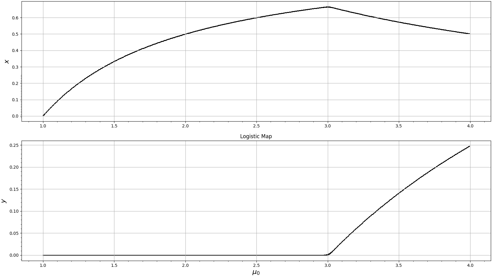
(a)

(b)

Figure 1: Competitive behavior and Lyapunov exponents of Normal.

3.2 Standard

Figure 2(a) shows bifurcation diagram and Lyapunov exponents of Standard. Our model shows that even with nonzero initial population and nonzero inter-species relationships of $\alpha$, $\beta$, and $\gamma$, we may still acquire flip bifurcation for $1$D logistic equation[39] for the prey at the absence of the predator. A flip bifurcation is a counterpart in discrete dynamic system to describe the concept of periodic doubling in the continuous dynamic system[40].

Figure 2(b) shows the Lyapunov exponents. Rosenstein algorithm did not show results in in this case, because singular value decomposition did not converge when doing linear least squares, meaning that positive or negative infinity appeared when we tried to deal with pseudo-inverse matrix. Eckmann Y cannot work, either, for $y=0$ in the whole range. We may see that for overall trend of $\lambda_{x}$, both algorithms have $\lambda_{x}<0$ for $\mu_{0}<3.0$, whereas $\lambda_{x}$ has both positive and negative values for $\mu_{0}>3.5$. It is widely accepted[41] that values of Lyapunov exponents occur interchangeably between positive and negative infer chaos, which is consistent with the shaded area in Figure 2(a). Another inconsistency occurs with $3.0<\mu_{0}<3.5$ with $\lambda_{x}>0$ for Equation but $\lambda_{x}<0$ for Eckmann X, where $x$ exhibits a flip bifurcation from $2$-cycle into $4$-cycle. Nevertheless, this inconsistency may not be a problem for us to distinguish chaos from happening. There is a break around $\mu_{0}=2$ for Eckmann X in both $\lambda_{x}$ and $\lambda_{y}$, at which Equation shows a deep trench in $\lambda_{x}$. Also, near $\mu_{0}\approx 1.245$, Equation shows a smaller trench while Eckmann X produces a rising tail.

Figure 3 studies the population in the course of time (iteration) at $\mu_{0}$ equal to $2.700$ ($1$-cycle), $3.000$ ($2$-cycle where the flip bifurcation occurs) and $3.500$ ($4$-cycle), $3.700$ (at which the system goes into chaos), $3.845$ (the system going back to more stable $3$-cycle), and $3.945$ (where the system returns to chaos again) in the successive order. Zero predator population is obtained throughout course of time.

Figure 4 studies topological types of fixed points. Plots of imaginary or real part of eigenvalues in Eq.(22) were evaluated at the fixed points $E^{\prime}_{1}$ in Eq.(23b) (as shown in the upper row), $E^{\prime}_{2}$ in Eq.(23c) (as shown in the middle row), and $E^{\prime}_{3}$ in Eq.(23d) (as shown in the bottom row). Color-bar at the right-hand side stands for various growth rate $\mu_{0}$, while circles with four different sizes in the legend represent, from the smallest to the biggest, topological types of sink, source, saddle, and non-hyperbole. We may see that $\omega_{0}$ and $\omega_{1}$ at the fixed points $E^{\prime}_{1}$ were pure real numbers with absolute values greater than $1$, making the fixed point a source for all $\mu_{0}$. While $\omega_{0}$ and $\omega_{1}$ at the fixed points $E^{\prime}_{2}$ were also pure real numbers, the absolute values vary across $1$, making the fixed point $E^{\prime}_{2}$ topological types of sink, source, and saddle, with possible non-hyperboles occurring at either low $\mu_{0}=1$ or high $\mu_{0}=3.75$ if we apply Theorem 2.$3$(d).

Figure 5 shows absolute values of eigenvalues $\omega_{0}$ and $\omega_{1}$ on fixed points $E^{\prime}_{1}$, $E^{\prime}_{2}$ and $E^{\prime}_{3}$. Topological types of fixed points may be double-checked more straightforwardly with the figure. The first column shows that $E^{\prime}_{1}$ is a source because $\omega_{0}$ and $\omega_{1}$ are always greater than $1$. The second column demonstrates that $E^{\prime}_{2}$ are a sink when $\mu_{0}<2.141$, and when $2.141<\mu_{0}<3$, $E^{\prime}_{2}$ is a saddle. Non-hyperboles can also be examined at $\mu_{0}=1$ for $E^{\prime}_{2}$, at $\mu_{0}=3$ for $E^{\prime}_{2}$ (in both cases $\omega_{0}=1$ and $\omega_{1}\neq 1$), and at $\mu_{0}=3.75$ for $E^{\prime}_{2}$ and $E^{\prime}_{3}$ (in which $\omega_{0}\neq 1$ and $\omega_{1}=1$). That $\mu_{0}=3.75$ is located in chaos region, making the fixed point vulnerable to nonlinear terms in the dynamic system. At last, when $\mu_{0}>3$, $E^{\prime}_{2}$ is a source.

Figure 6 shows phase portrait and phase space diagram about Standard. $\mu_{0}$ values are represented by the color bar at the right-hand side. Figure 6(a) refers to phase portrait, where topological types are also shown in the legend. An isolated initial coordinate ($0.1,0.50$) marked as a source at the upper-left corner. Flip bifurcation occurs at ($0.665,0,000$). No limit circles were found in the flip bifurcation. The oblique black straight line, starting from ($0.732,0.000$) to ($0.689,0.062$), consisting of fixed points $E^{\prime}_{3}$ that is enclosed by a thicker yellow cloak indicates that, along the axis, $E^{\prime}_{3}$ is a saddle, with nonzero $y$ values. This result seems to contradict to the previous one, saying that predator population is always zero. However, since our initial population is ($x,y$)=($0.1,0.5$), it does not lie in the above range. Therefore, the system with the chosen inter-species constants is not attracted by the saddle points along the oblique black line, confirming that with none-zero initial population of the predator and non-zero inter-species constants, the predator could appear, but only for a while. Afterwards, the predator dies out in the course of time, leaving the prey to be the only surviving species in the paradisaic. This observation may explain why the predator species may not survive long in some specific ecological system. Further, Figure 6(b) is phase space diagram for the prey. It is meaningless to discuss phase space diagram for the predator because there are only two points, ($0.0,0.0$) and ($0.5,-0.5$), in this case.

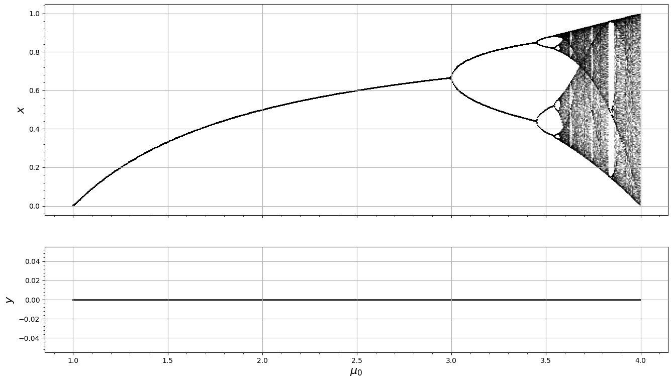
(a)

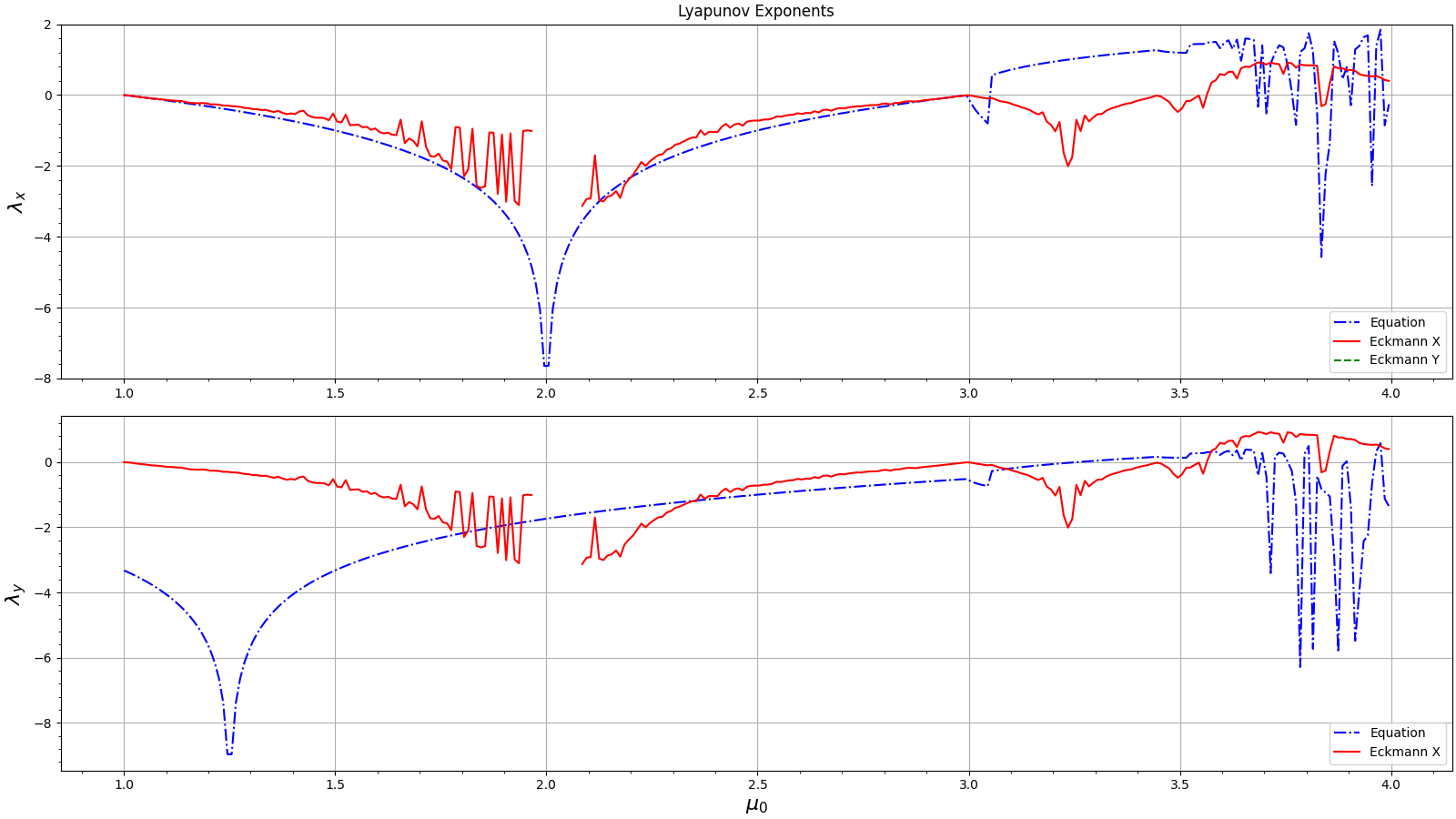
(b)

Figure 2: Bifurcation diagram and Lyapunov exponents of Standard.

(a)

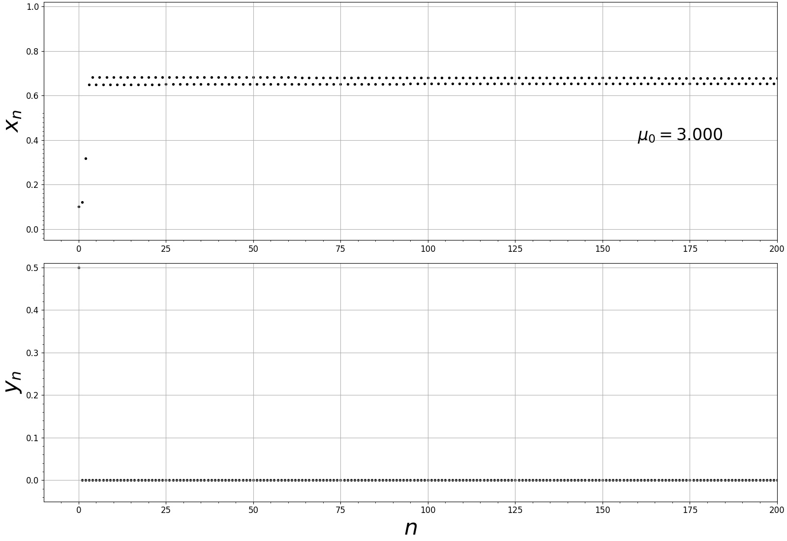
(b)

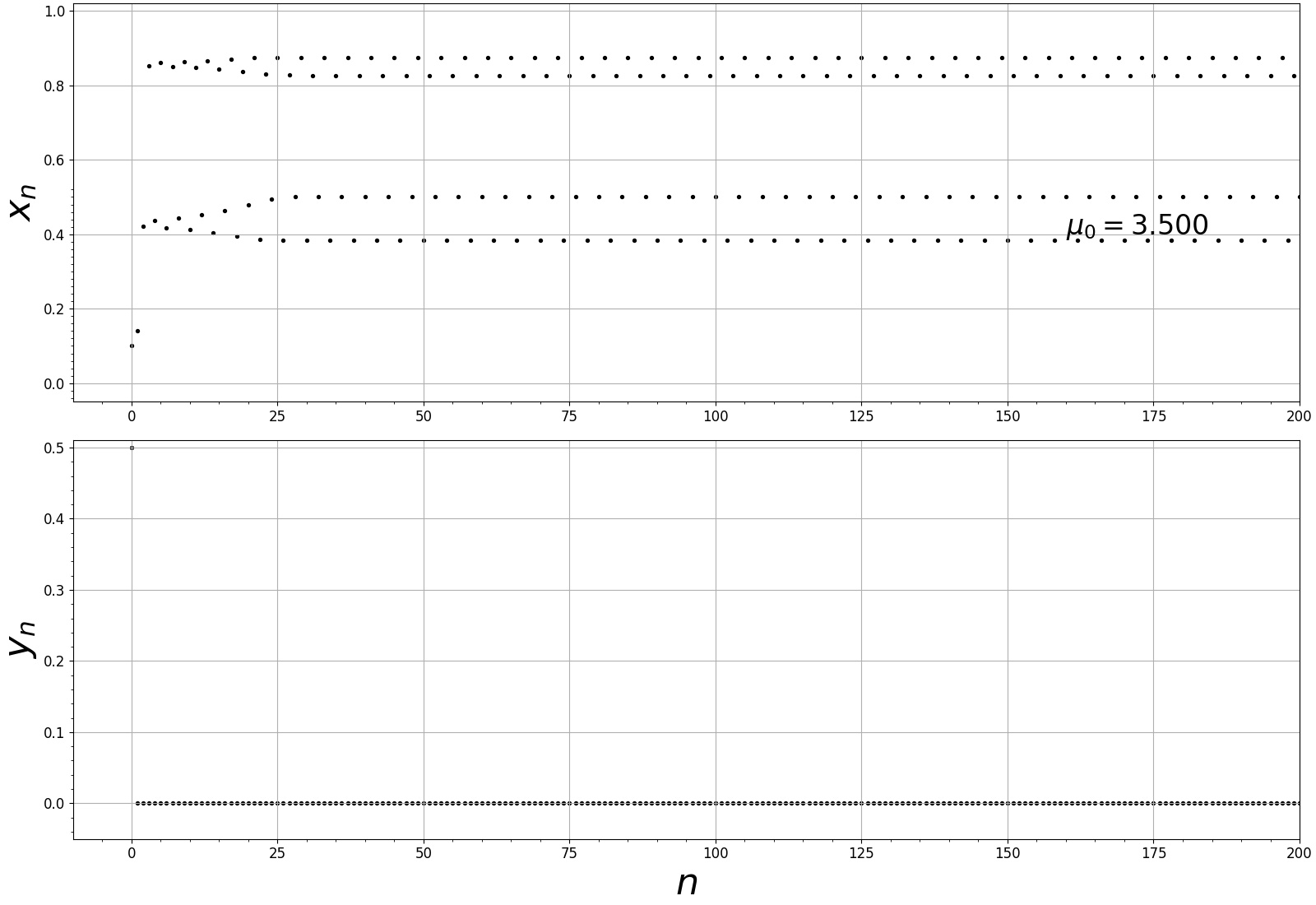
(c)

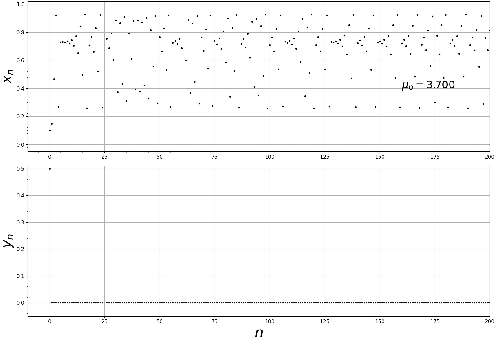
(d)

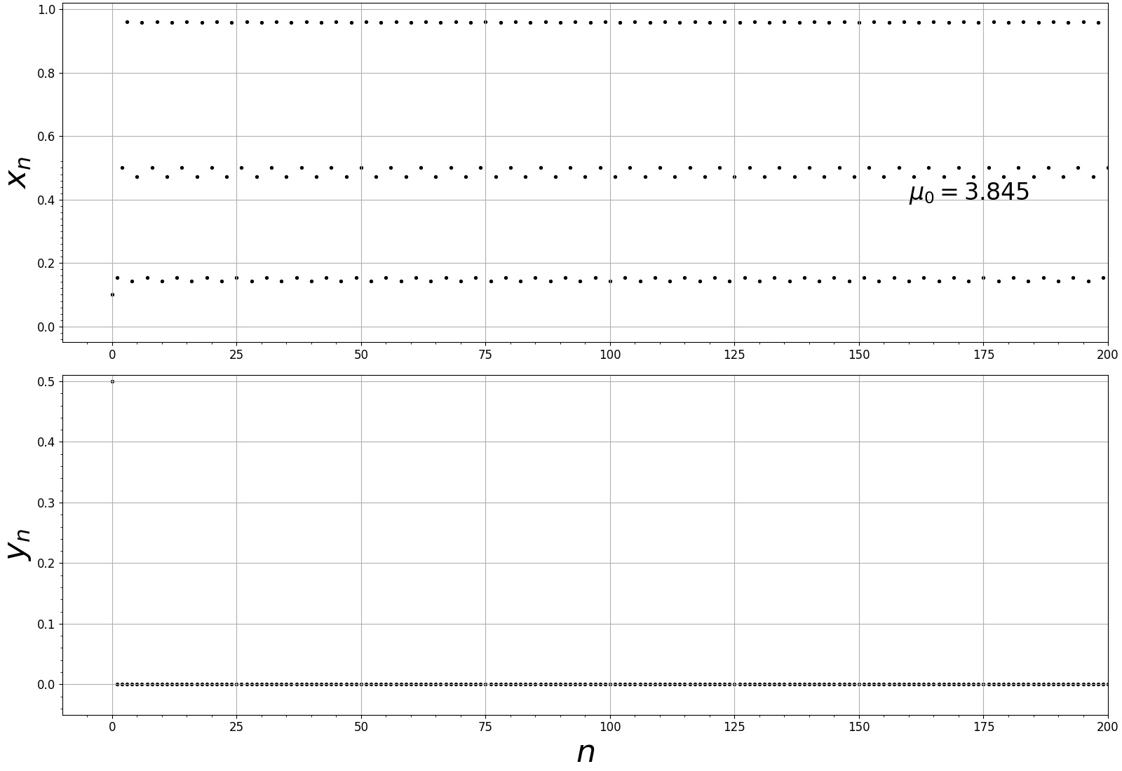
(e)

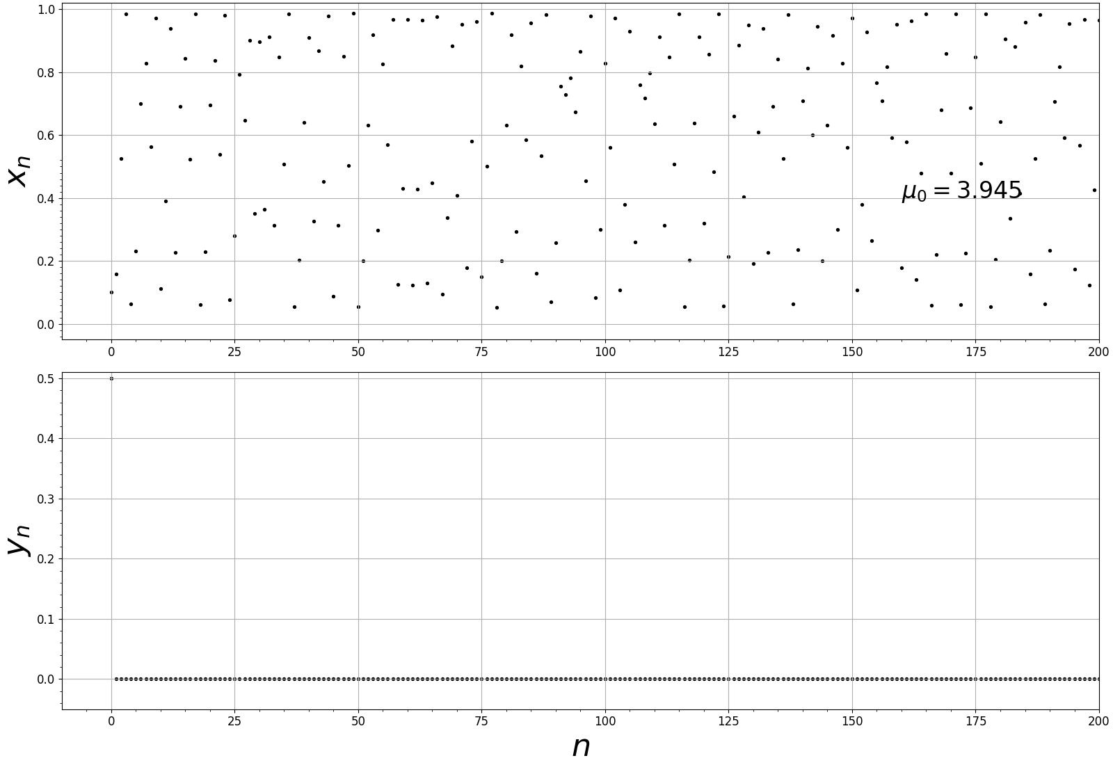
(f)

Figure 3: Population vs. iteration of Standard.

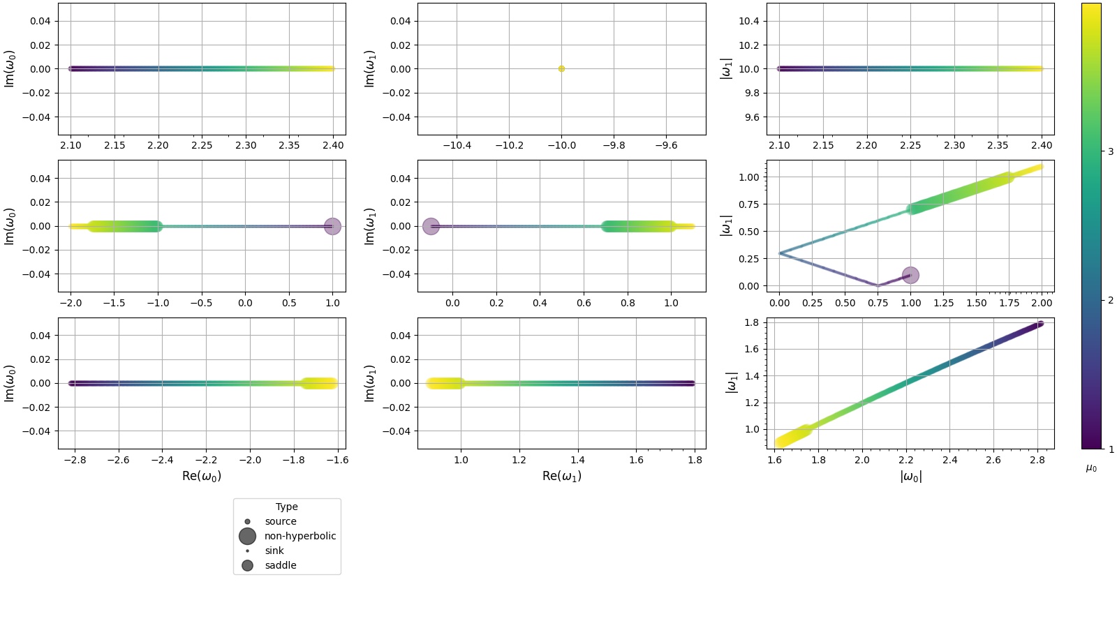
Figure 4: Analysis on eigenvalues for the case of Standard. Eigenvalues described in Eq.(22) for fixed points $E^{\prime}_{1}$ (Eq.(23b)), $E^{\prime}_{2}$ (Eq.(23c)), and $E^{\prime}_{3}$ (Eq.(23d)) are plotted in the upper row, middle row, and lower row, respectively. Types of topology are indicated with circles of various sizes. Color bar stands for different $\mu_{0}$.

.

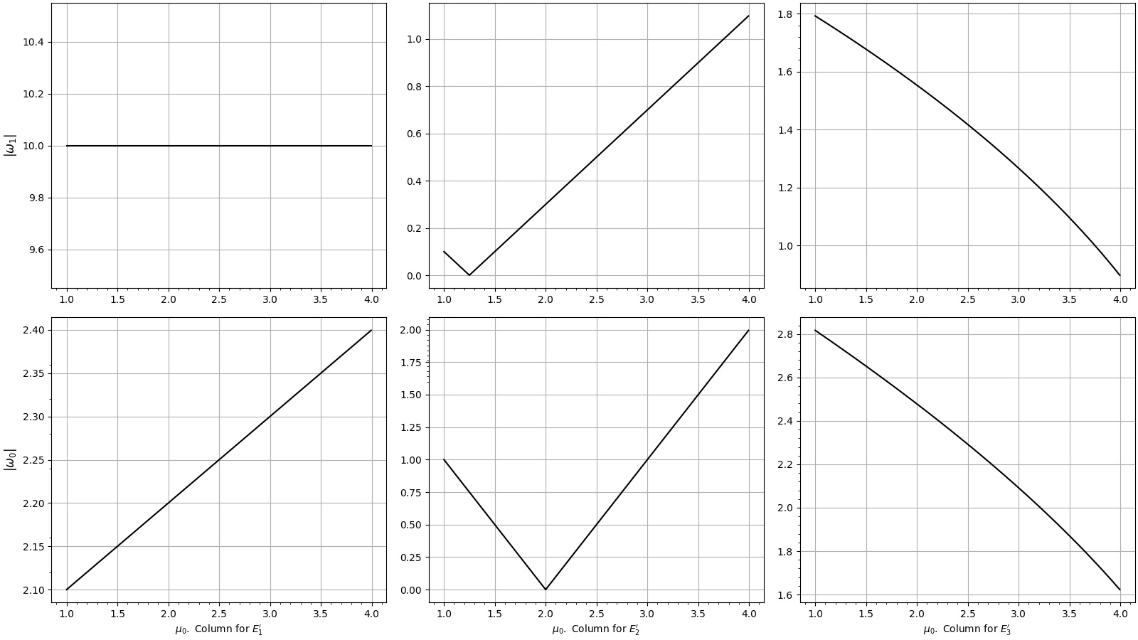
Figure 5: Absolute values of eigenvalues vs. growth rate at fixed points for Standard. Prominent coordinates that help us understand stability and distinguish the topological type about a fixed point are recorded as follows. Upper middle panel: ($1.244,0.000$), and ($3,75,1,00$). Upper-right corner panel: ($3.75,1.00$). $E^{\prime}_{2}$ and $E^{\prime}_{3}$ are both non-hyperbolic at $\mu_{0}=1$, $3$, and $3.75$.

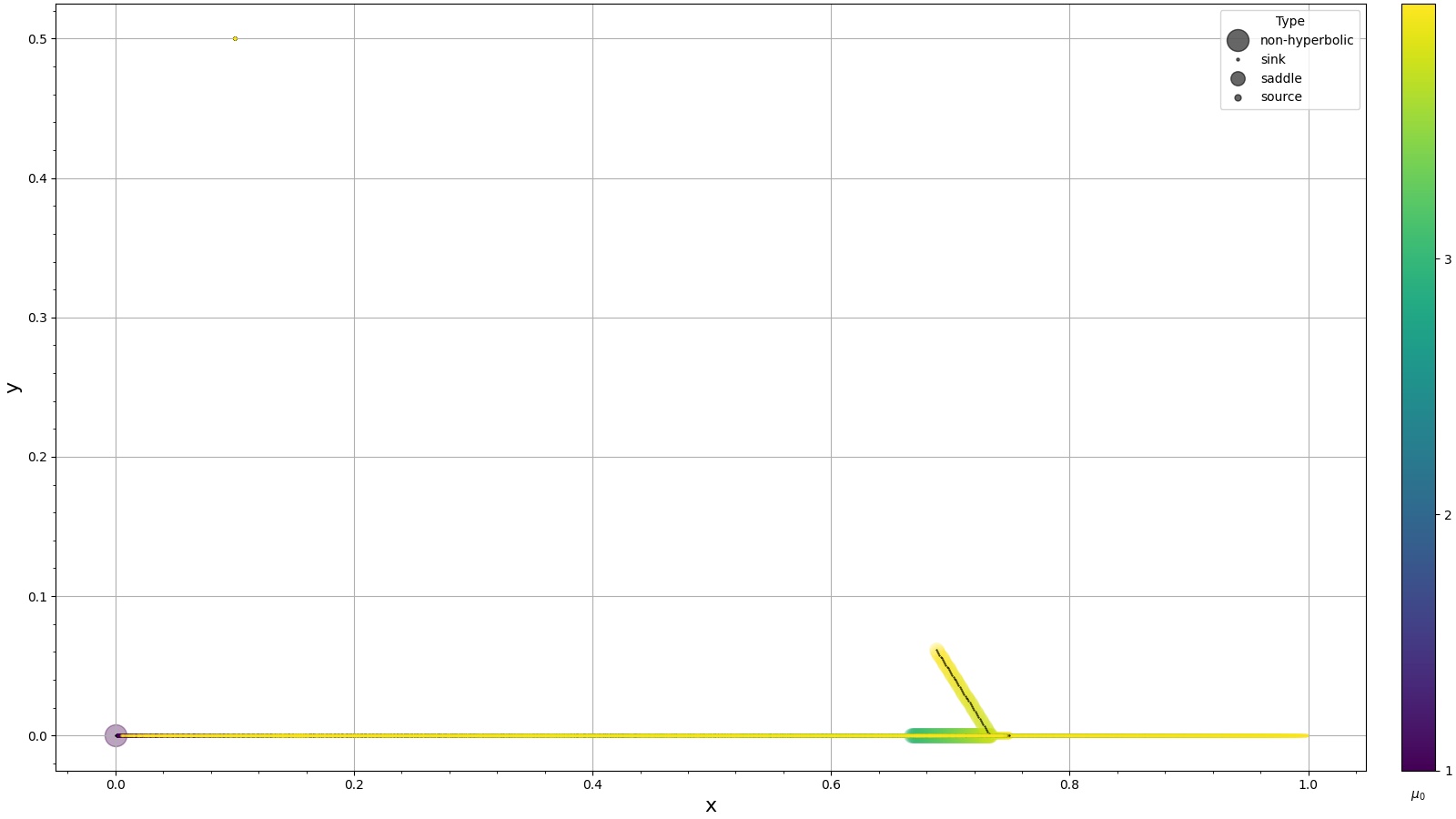
(a)

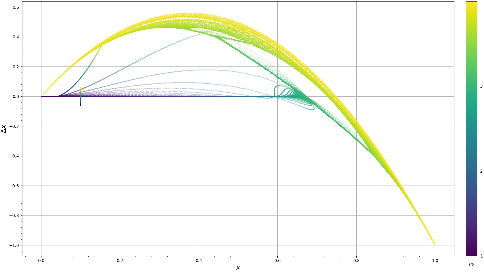
(b)

Figure 6: Analysis on phase portrait and phase space diagram about Standard. Topological types of sink, source, saddle and non-hyperbole are represented with different sizes from the smallest to the largest as shown in the legends. Oblique black line in Figure 6(a) indicates saddle fixed points, demonstrating that the predator cannot survive long in the ecological system. Figure 6(b) shows the phase space of $x$. Phase diagram of the predator is not shown here, because it only contains two points ($0.0,0.0$), and ($0.5,-0.5$), which makes the figure boring.

3.3 Paraclete

Figure 7(a) represents two sets of overlapping bifurcation diagrams: one is the Standard, the other with vorticella-shaped, which starts to appear after $\mu_{0}=2.29$. Between $2.29<\mu_{0}<2.45$, shaded regions appearing vertically with gaps are not chaos but transient states of population. At $\mu_{0}=3.256$, the vorticella-shaped has bifurcation that start to be chaotic, at which we would explain later that it should be classified as Neimark-Sacker bifurcation, and mingles together with the flip bifurcation of Standard after $\mu_{0}=3.46$, at which the four-cycles occurs.

Figure 7(b) shows the Lyapunov exponents for Paraclete. For the same reason in Standard, Rosenstein algorithm did not show results in in this case, either. We may see that for overall trend of $\lambda_{x}$, algorithms of both Equation and Eckmann X have $\lambda_{x}<0$ for $\mu_{0}<3.0$, whereas $\lambda_{x}$ has both positive and negative values for $\mu_{0}>3.0$, inferring chaos. Eckmann Y only shows a small portion, not spectrum, because $y=0$ for $\mu_{0}<2.29$ leads to failure on producing full spectrum of both $\lambda_{x}$ and $\lambda_{y}$. Therefore, where we may see only some segment of $\lambda_{x}$ after $\mu_{0}>3.0$ that almost overlaps with the curve of Eckmann X. Inconsistency also occurs at low growth rate in $\lambda_{y}$ spectrum, for Equation shows stern-drooping tails while Eckmann X shows a raising-up one.

Figure 8 studies the population in the course of time (iteration) at $\mu_{0}$ equal to $2.790$ (stable population), $3.025$ ($2$-cycle), $3.255$ (at which Neimark-sacker bifurcation is on the way), $3.460$ ($4$-cycle), $3.845$ ($3$-cycle in Standard), and $3.945$ (chaos region) in the successive order.

Figure 9 studies topological types of fixed points. Plots of imaginary or real part of eigenvalues in Eq.(22) were evaluated at the fixed points $E^{\prime}_{1}$ in Eq.(23b) (as shown in the upper row), $E^{\prime}_{2}$ in Eq.(23c) (as shown in the middle row), and $E^{\prime}_{3}$ in Eq.(23d) (as shown in the bottom row). Color-bar at the right-hand side stands for various growth rate $\mu_{0}$, while circles with four different sizes in the legend represent, from the smallest to the biggest, topological types of sink, source, saddle, and non-hyperbole. We may see that $\omega_{0}$ and $\omega_{1}$ at the fixed points $E^{\prime}_{1}$ were pure real numbers with absolute values greater than $1$, making the fixed point a source for all $\mu_{0}$. While $\omega_{0}$ and $\omega_{1}$ at the fixed points $E^{\prime}_{2}$ were also pure real numbers, the absolute values vary across $1$, making the fixed point $E^{\prime}_{2}$ topological types of sink, source, and saddle, with only one possible non-hyperbole occurring at $|\omega_{0}|=1$.

Figure 10 shows absolute values of eigenvalues $\omega_{0}$ and $\omega_{1}$ on fixed points $E^{\prime}_{1}$, $E^{\prime}_{2}$ and $E^{\prime}_{3}$. Topological types of fixed points may be double-checked more straightforwardly with the figure. The first column shows that $E^{\prime}_{1}$ is a source because $\omega_{0}$ and $\omega_{1}$ are always greater than $1$. The second column demonstrates that $E^{\prime}_{2}$ are a sink when $\mu_{0}<2.141$, and when $2.141<\mu_{0}<3$, $E^{\prime}_{2}$ is a saddle. At last, when $\mu_{0}>3$, $E^{\prime}_{2}$ is a source.

As we look closely into the third column, it shows that $E^{\prime}_{3}$ is non-hyperbolic at $\mu_{0}\approx 2.137$ for $\omega_{0}\neq 1$ and $\omega_{1}=1$, which is vulnerable to nonlinear terms in the dynamic system. It explains why the transient state under that growth rate is not shown in Figure 7(a). Also, bending points along curves plotted in the third-column figures demonstrate that transient states occur within $2.258<\mu_{0}<2.475$. More interestingly, the third column manifests that $E^{\prime}_{3}$ represents Neimark-Sacker bifurcation at $\mu_{0}=3.25636$ because of the following facts: first, $\omega_{0}$ and $\omega_{1}$ are complex conjugates with modulus $1$, and second, as $\mu_{0}$ varies across $3.25636$ from smaller to larger value, topological type of $E^{\prime}_{3}$ changes from a sink (stable) to a source (unstable)[19].

Figure 11 shows phase portrait and phase space diagram about Paraclete. $\mu_{0}$ values are represented by the color bar at the right-hand side. Figure 11(a) refers to phase portrait, showing Neimark-Sacker bifurcation established at ($0.352,0.068$) with $\mu_{0}\approx 3.256$ at the center of limit circles. Black straight lines indicate oblique axis consisting of $E^{\prime}_{3}$, including sink and source, and horizontal axis composed of $E^{\prime}_{2}$, including source and saddle, under different $\mu_{0}$. Topological types are also shown in the legend. Dots with larger $\mu_{0}$ representing chaos spread outside around the limit circles. Figure 11(b) is phase space diagram for the prey centered at ($0.352,0$) and Figure 11(c) refers to phase space diagram for the predator centered at ($0,0.068$). Not surprisingly, the center of limit circles in Figure 11(b) has the same $x$ value as that of Figure 11(a). Similarly, same $y$ value for the center of limit circles in Figure 11(c) and in Figure 11(a).

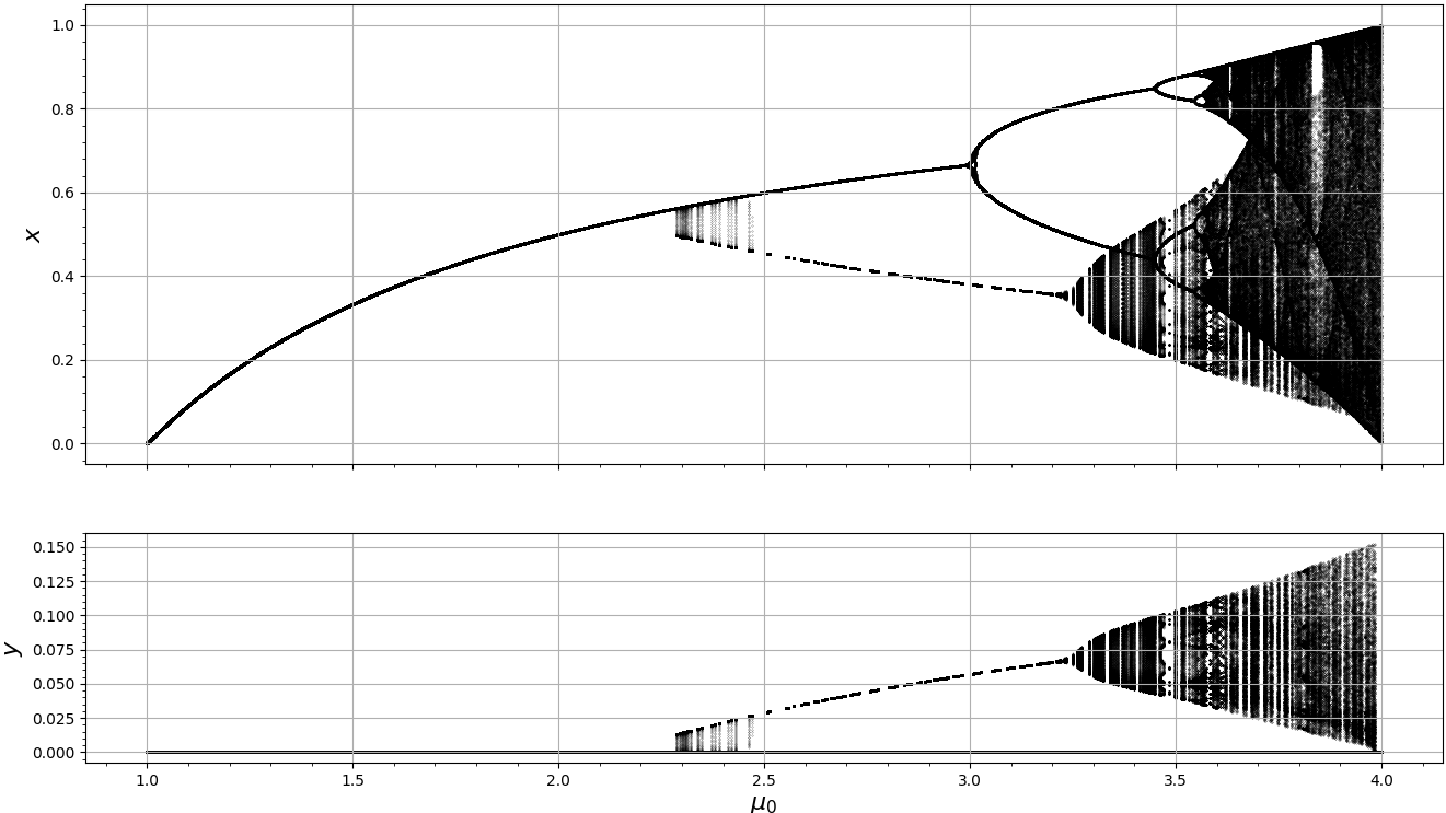
(a)

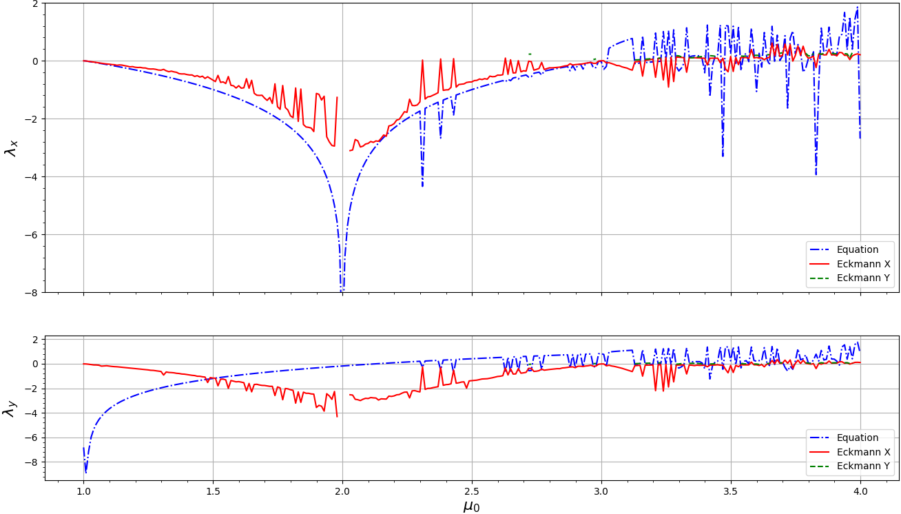
(b)

Figure 7: Bifurcation diagram and Lyapunov exponents of Paraclete.

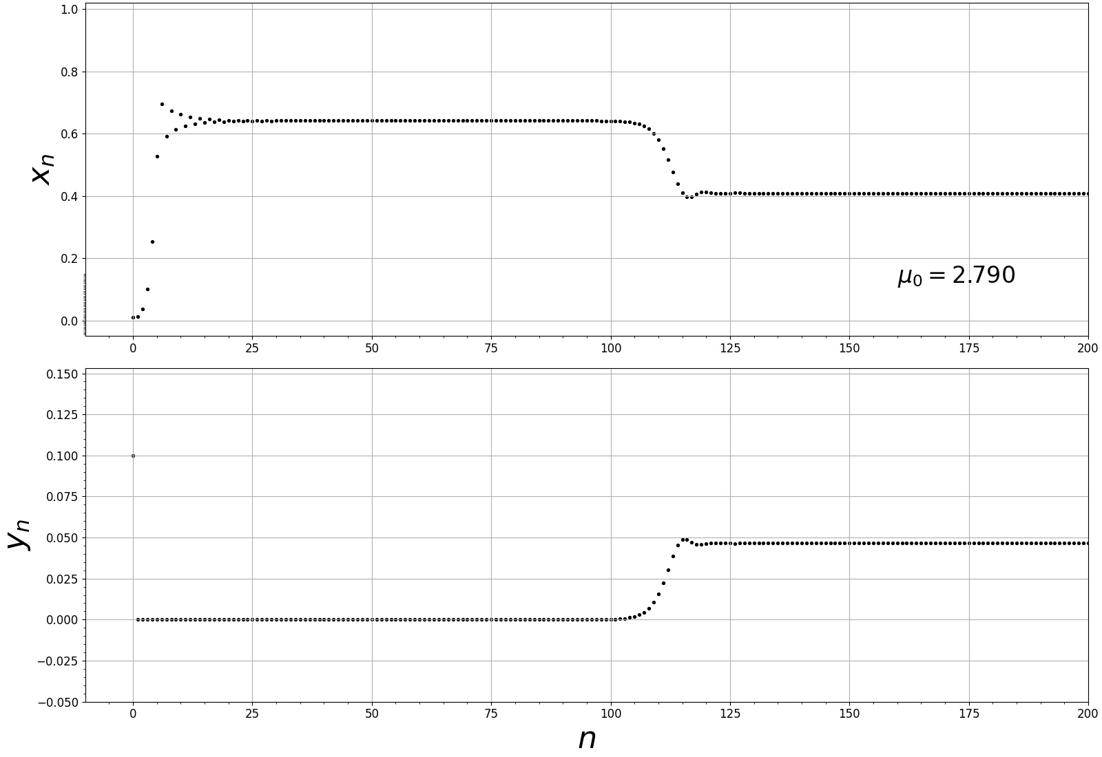
(a)

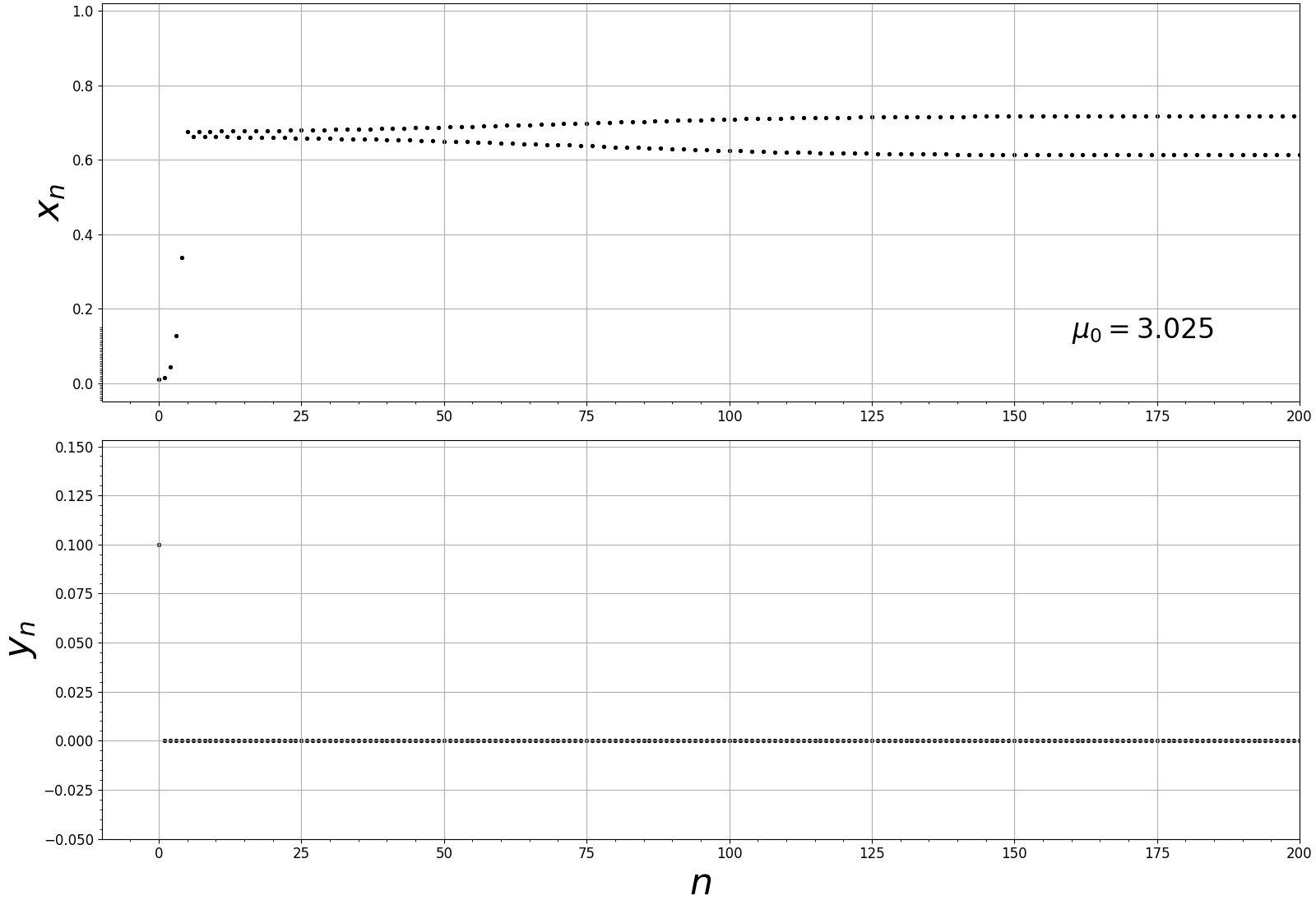
(b)

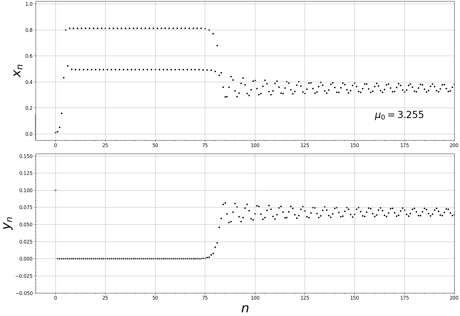
(c)

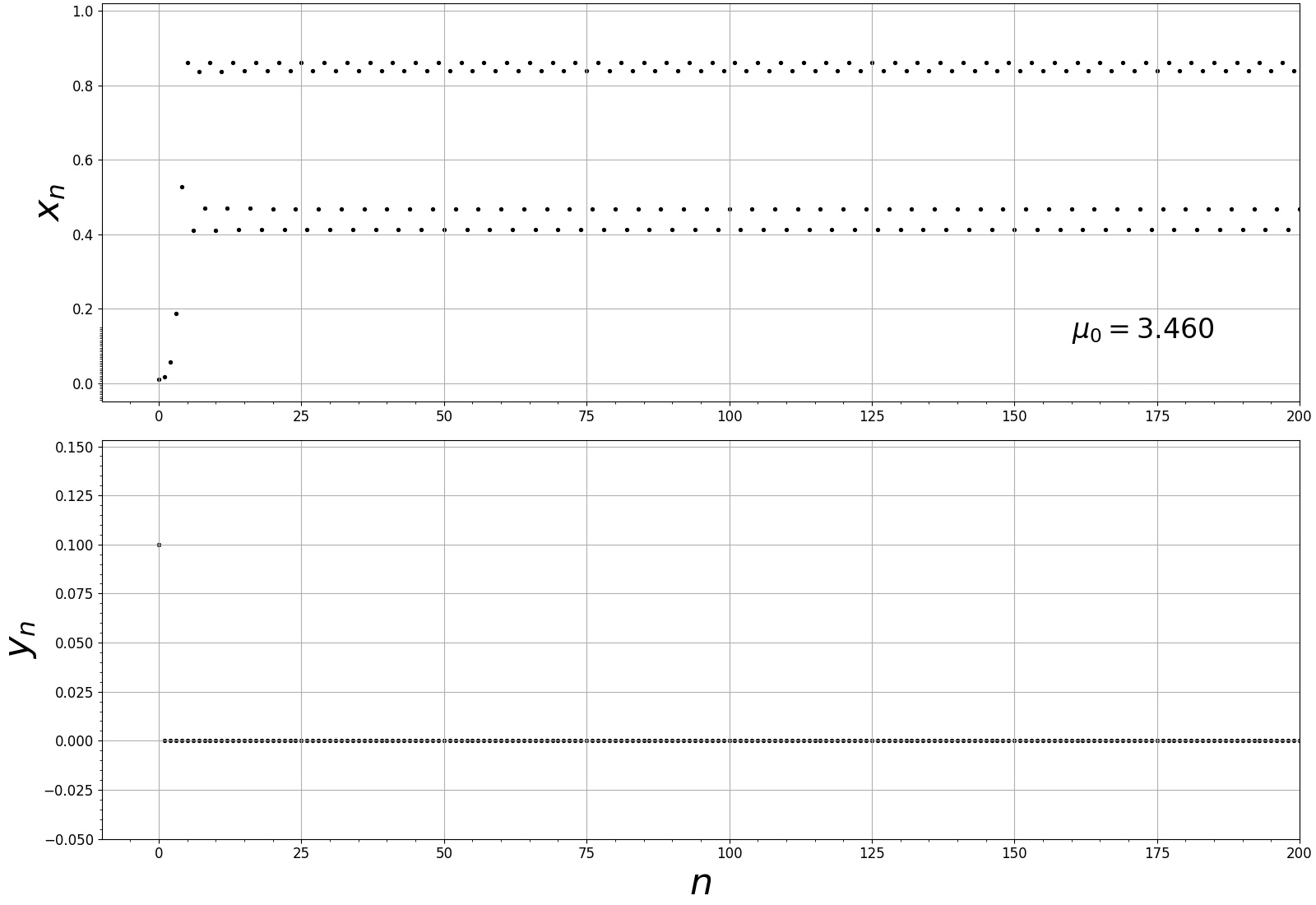
(d)

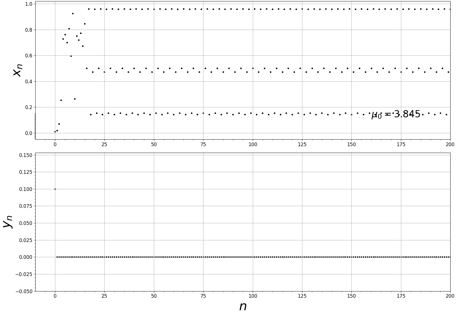
(e)

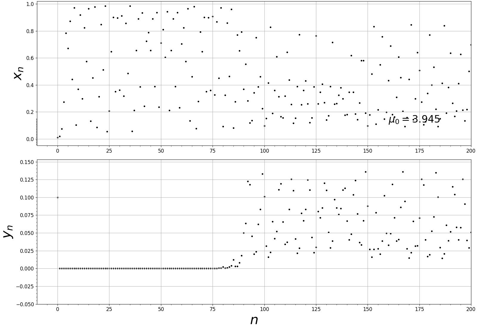
(f)

Figure 8: Population vs. iteration of Paraclete.

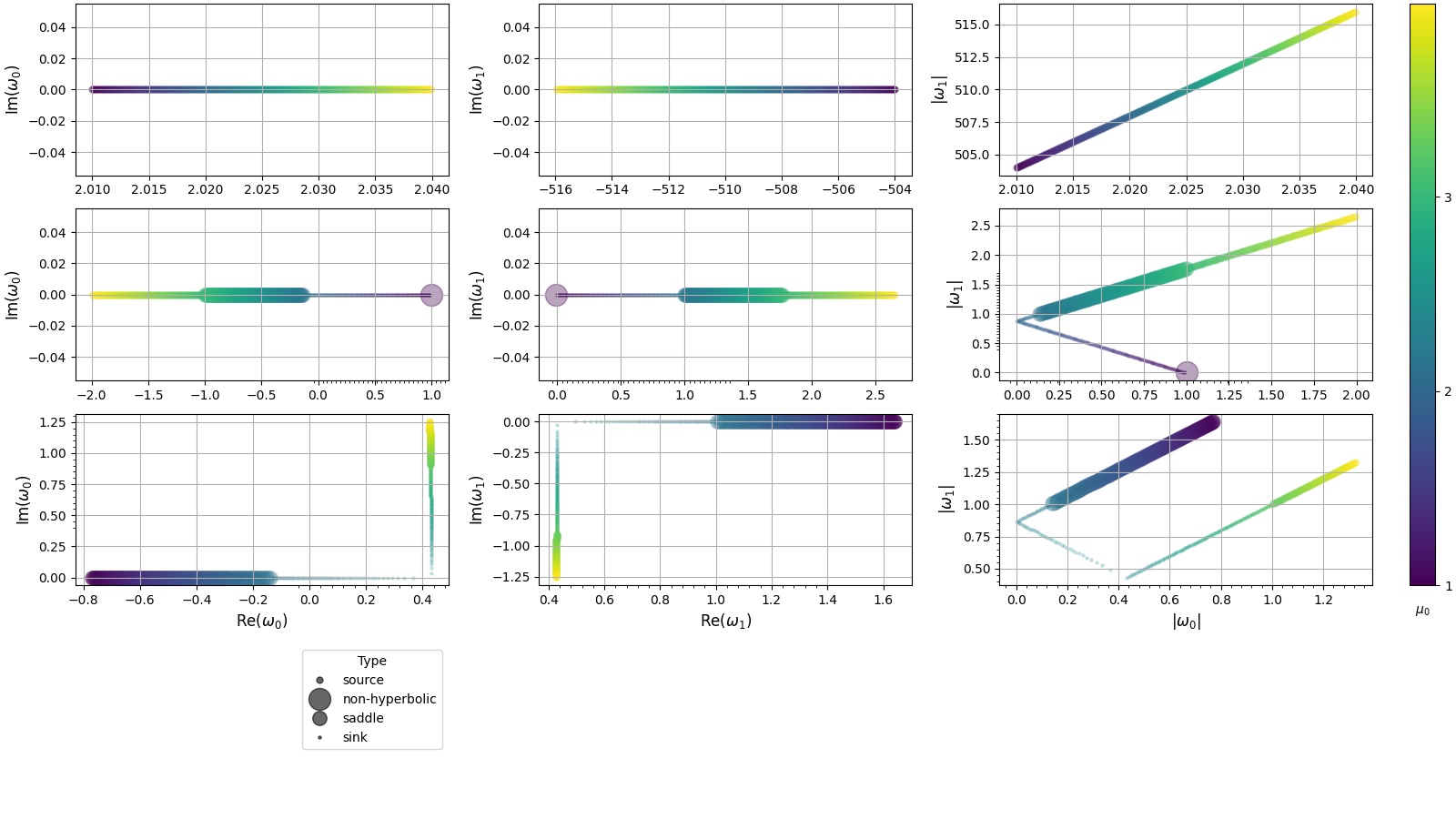
Figure 9: Analysis on eigenvalues for the case of Paraclete. Legends have the same meaning described in Figure 4.

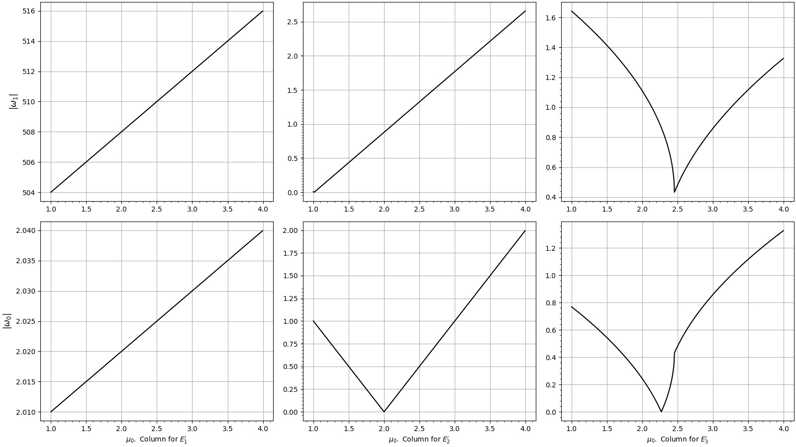
Figure 10: Absolute values of eigenvalues vs. growth rate at fixed points for Paraclete. Important coordinates: Upper middle panel ($2.14,1.00$). Upper-right corner panel ($2.137,1.000$), ($2.457,0.440$), and ($3.256,1.000$). Lower-right corner panel ($2.258,0.000$), ($2.475,0.427$), and ($3.256,1.000$).

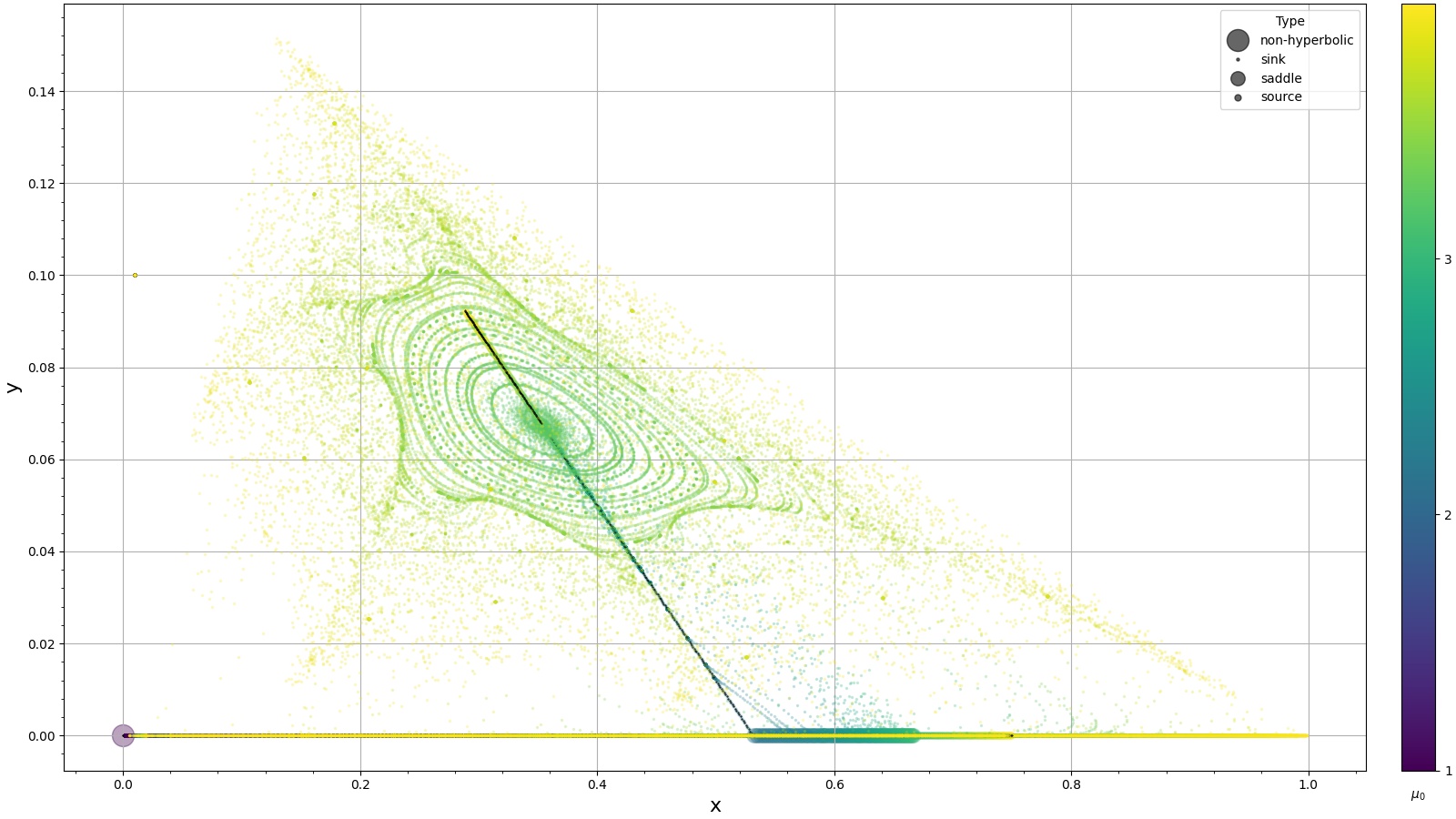
(a)

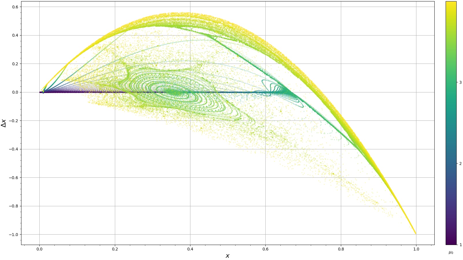
(b)

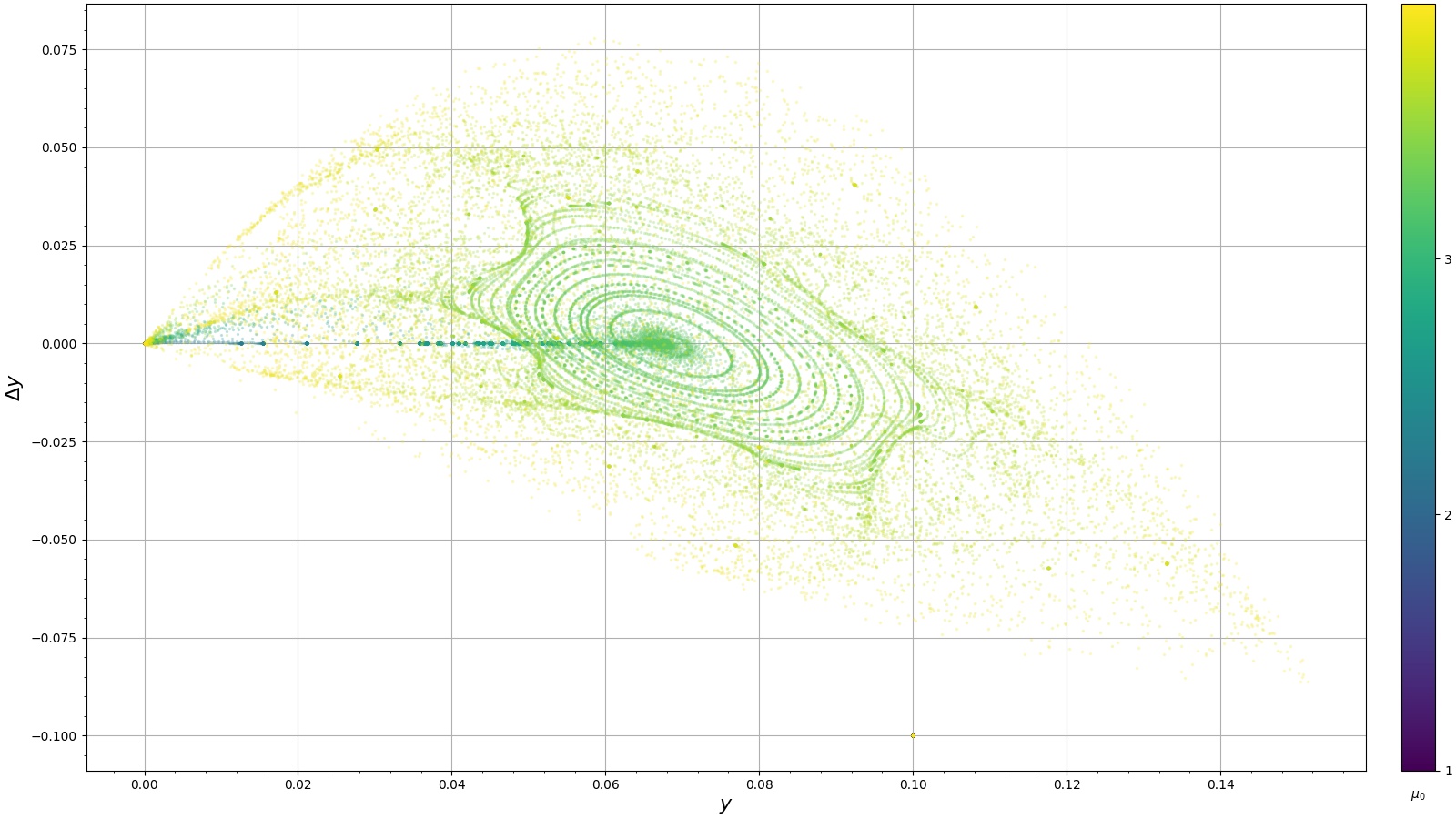
(c)

Figure 11: Analysis on phase portrait and phase space diagram about Paraclete. (11(a))Phase portrait shows Neimark-Sacker bifurcation established at ($0.352,0.068$) with $\mu_{0}\approx 3.256$ located at the center of limit circles. Oblique axis and horizontal axis consisting of $E^{\prime}_{3}$ and $E^{\prime}_{2}$ with different $\mu_{0}$, respectively. We may see from the legend that topological types of $E^{\prime}_{3}$ are mostly sink and source, while those of $E^{\prime}_{2}$ are mostly source and saddle. Phase portrait and phase space diagram for the prey have same $x$ in (11(b)) for the center limit circle. Similarly, phase portrait and phase space diagram for the predator have same $y$ in (11(c)) for the center limit circle.

3.4 Extinction

Figure 12(a) shows the bifurcation diagram of Extinction. There is a flip bifurcation for $x$ around $\mu_{0}\approx 2.99$; however, the $2$-cycle collides at $\mu_{0}\approx 3.165$ and returns back to $1$-cycle. Shaded regions between $3.165<\mu_{0}<3.434$ for $x$ and $3.10<\mu_{0}<3.343$ for $y$ do not refer to chaos but belong to transient states. Afterwards, the bifurcation diagram goes back to Normal for both $x$ and $y$, and represent pleasant conditions of predictable values before $x$ goes into $3$-cycle at $\mu_{0}\approx 3.828$ as in Standard, where $y$ drops to zero cliff-fallingly at $\mu_{0}\approx 3.824$, manifesting to extinction of the predator for the prey is around the $3$-cycle state. Fortunately, there could be still few little chances for the predator to survive at ($\mu_{0},y$) = ($3.845,0.219$), ($3.887,0.226$), and ($3.897,0.228$), where we may see three isolated fixed points appear with a vertical tail of transient states. When the prey becomes fully chaotic, the predator population reduces back to zero dramatically again, and never has any further opportunity to rise back. This astonishing phenomenon could be the most profound finding in the study, which states that the prey in chaos generated by overpopulation of the predator would erase the entire predator species.

Figure 12(b) shows Lyapunov exponents for Extinction that is similar to those in Figure 1(b), except for the regions at $3.0<\mu_{0}<3.18$ and $\mu_{0}>3.86$, the former showing a bum by Equation, which is also the same region for the prey to be in $2$-cycle, and the latter presenting chaos for $x$ and extinction for $y$. Discrepancy appears for Eckmann Y that is different from the other when $\mu_{0}<1.662$, where it shows a decreasing tail while the other algorithms show an increasing trend. Unlike Figure 1(b), whose results show that Eckmann X is always in between Rosenstein and Eckmann Y in the range of $1.5<\mu_{0}<3.0$, Figure 12(b) shows more intertwines at $\mu_{0}=1.886$ for $\lambda_{x}$, and at $\mu_{0}=1.717$ and $\mu_{0}=1.891$ for $\lambda_{y}$. Similar to Figure 1(b), the four algorithms also divides into two groups of curves below $\mu_{0}=1.717$, with Rosenstein and Eckmann X going upward, together with Equation and Eckmann Y going downward.

Figure 13 shows population iteration of Extinction. As we can see, flip bifurcation starts at $\mu_{0}=3.000$ as in Figure(13(a)), while in Figure(13(b)) the two fixed points collide, and after transient states ($n>200$), they have tendency to merging into a single fixed point, as we explained earlier in Figure 12(a) on the characteristics about the shaded region between $3.165<\mu_{0}<3.434$ for $x$. We further demonstrate that at $\mu_{0}=3.500$ in Figure(13(c)), after transient($n>175$), bifurcation collapses to one. Furthermore, $3$-cycle is opened in $x$ at $\mu_{0}=3.84$, as indicated in Figure(13(d)), with extinction of $y$ at the exactly the same moment. However, a sunlight of survival for $y$ is shed on the window at $\mu_{0}=3.845$, as shown in Figure(13(e)), where the two species may still exist under predictable population. Finally, Figure 13(f) portends the predator extinction under chaos of the prey.

Figure 14 studied topological types of fixed points. Plots of imaginary or real part of eigenvalues in Eq.(22) were evaluated also at the three fixed points $E^{\prime}_{1}$, $E^{\prime}_{2}$, and $E^{\prime}_{3}$ as in Figure 4. We may see that $\omega_{0}$ at the fixed points $E^{\prime}_{1}$ is pure real numbers with absolute values greater than $1$, whereas $\omega_{1}$ keeps the value $-1000$ for all $\mu_{0}$, making the fixed point a source (unstable) for all $\mu_{0}$. While $\omega_{0}<1$ and $\omega_{1}>1$ at the fixed points $E^{\prime}_{2}$, the fixed point $E^{\prime}_{2}$ has a topological type of saddle, with possible non-hyperboles occurring at $|\omega_{0}|=1$ and $|\omega_{1}|=0$.

Stability of fixed points may also be examined in Figure 20. Figures at the first column shows that that $E^{\prime}_{1}$ is a source, for both eigenvalues have absolute values greater than $1$. In the second column, we see that $E^{\prime}_{2}$ changes its stability from a sink to source when $\mu_{0}$ varies at $3$, at which flip bifurcation occurs; meanwhile, $E^{\prime}_{3}$ changes from source to sink.

Figure 16 shows phase portrait and phase diagrams for Extinction. No limit circles are found in this particular case.

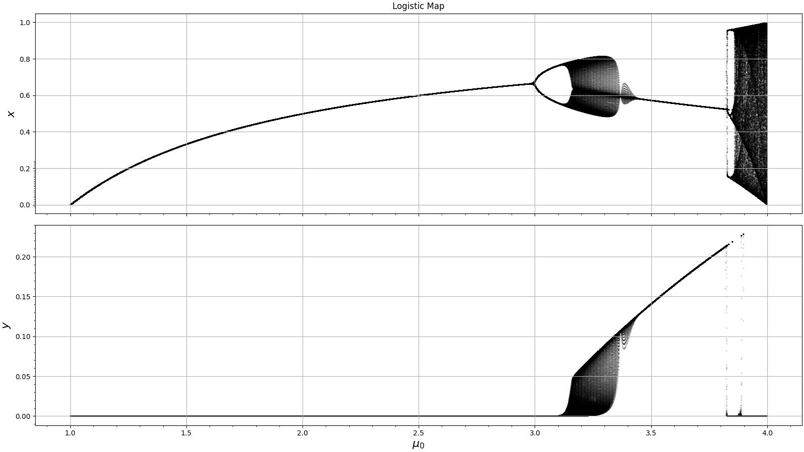
(a)

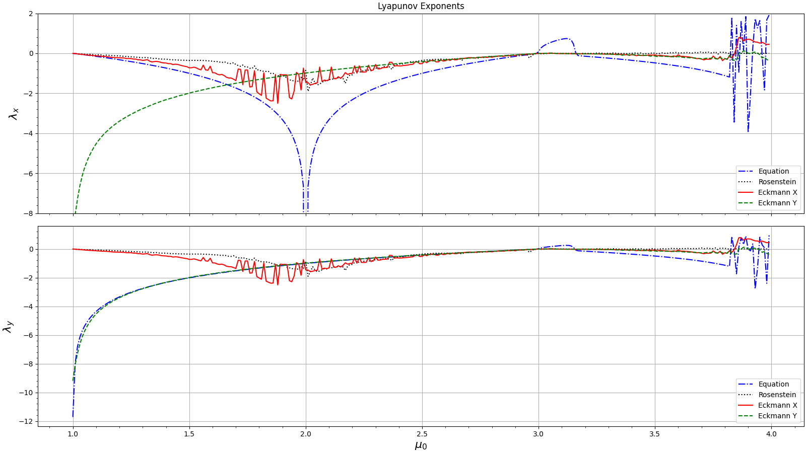
(b)

Figure 12: Bifurcation diagram and Lyapunov exponents of Extinction.

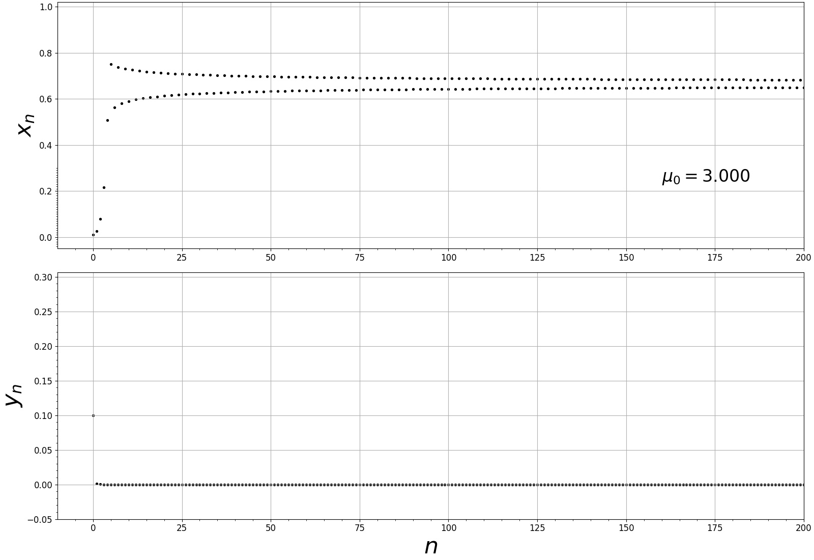
(a)

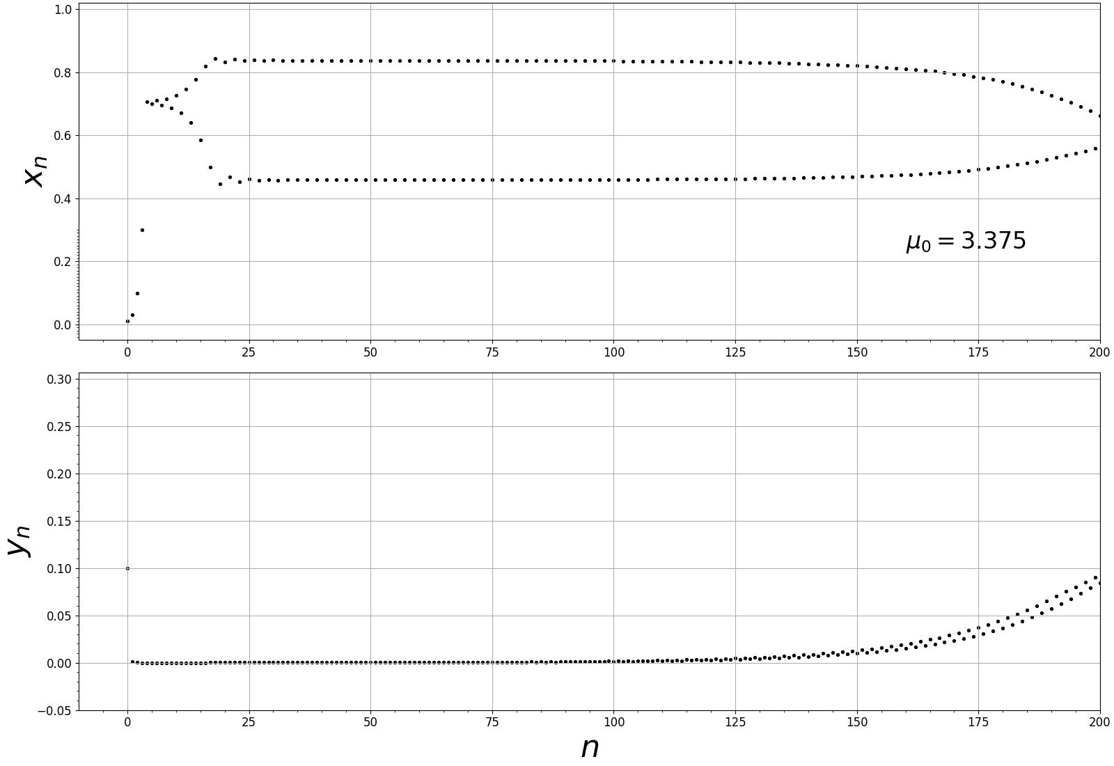
(b)

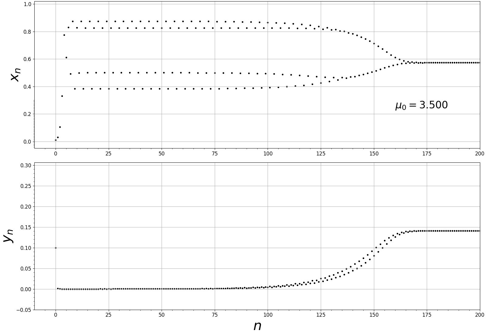
(c)

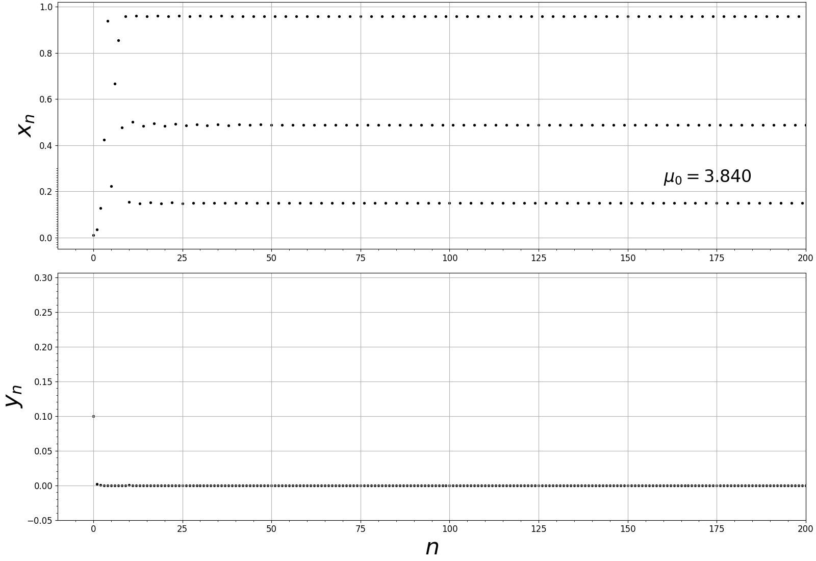
(d)

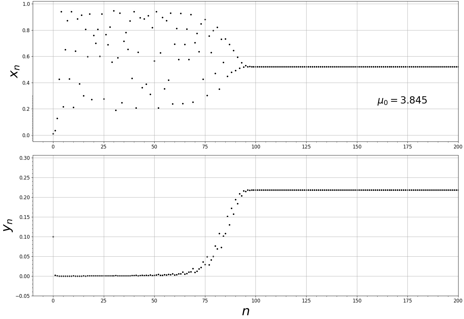
(e)

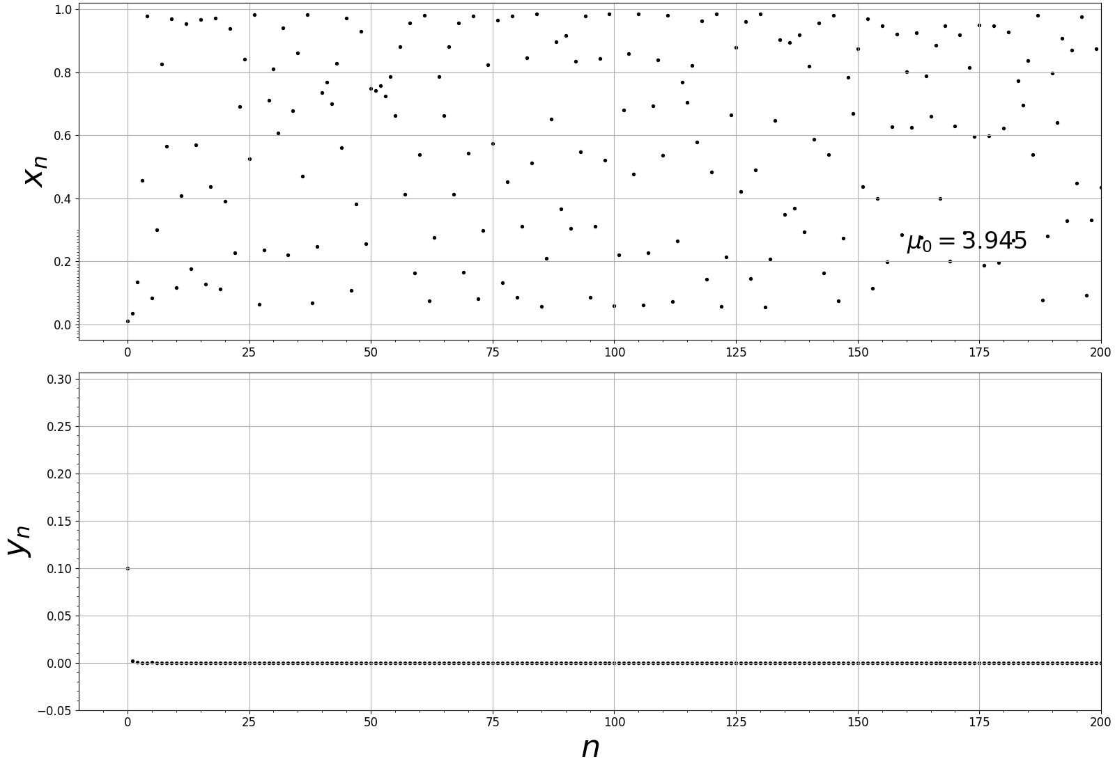
(f)

Figure 13: Population vs. iteration of Extinction.

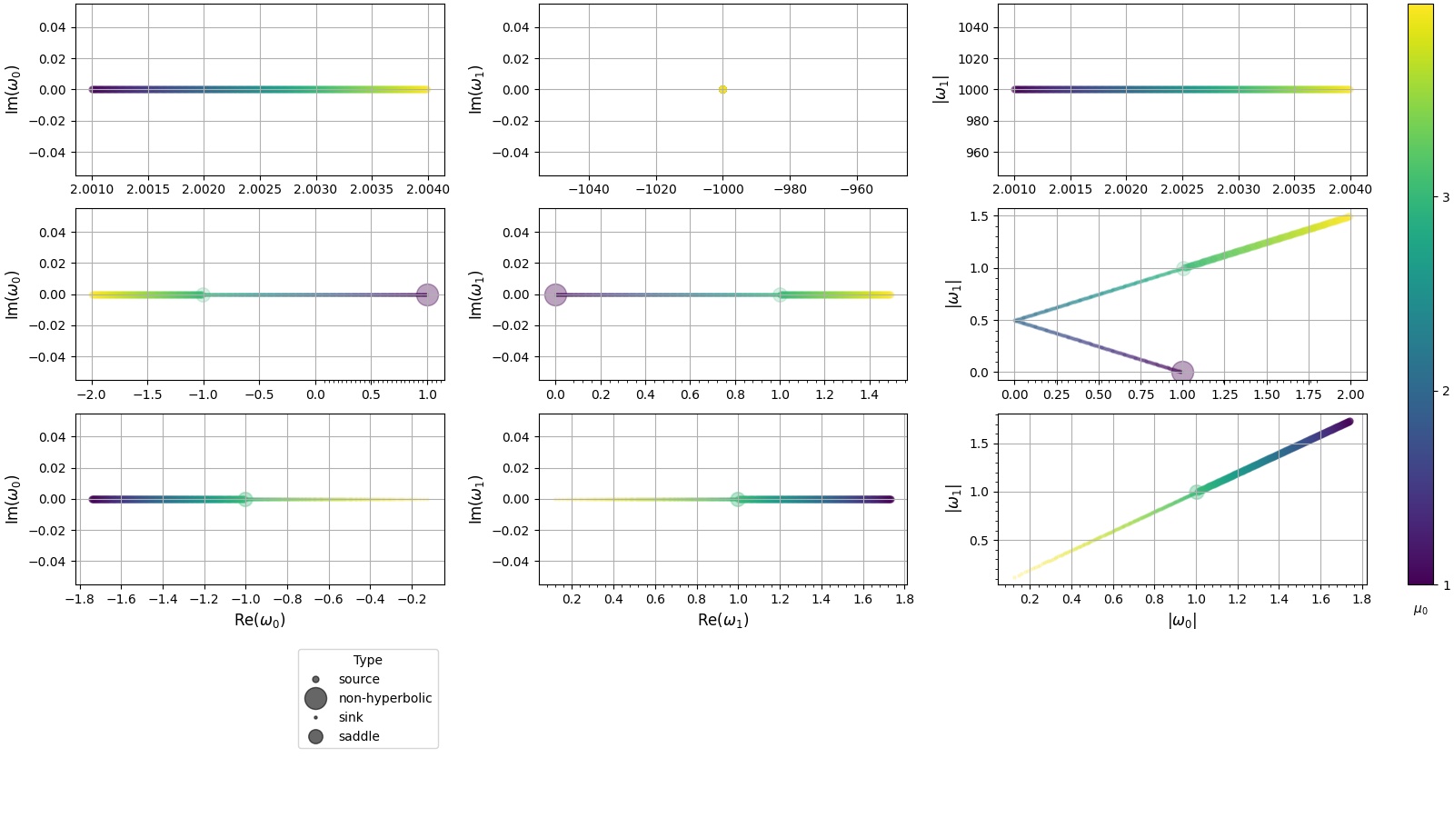
Figure 14: Analysis on eigenvalues for the case of Extinction. Legends have the same meaning described in Figure 4.

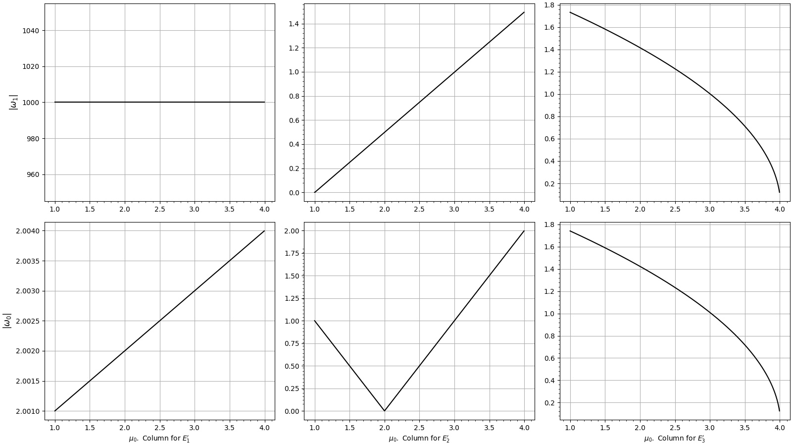
Figure 15: Absolute values of eigenvalues vs. growth rate at fixed points for Extinction. From the figures at the first column, it is clearly shown that $E^{\prime}_{1}$ is a source. Also, at $\mu_{0}=3$ where flip bifurcation occurs, $E^{\prime}_{2}$ changes its stability from a sink to source, whereas $E^{\prime}_{3}$ from source to sink.

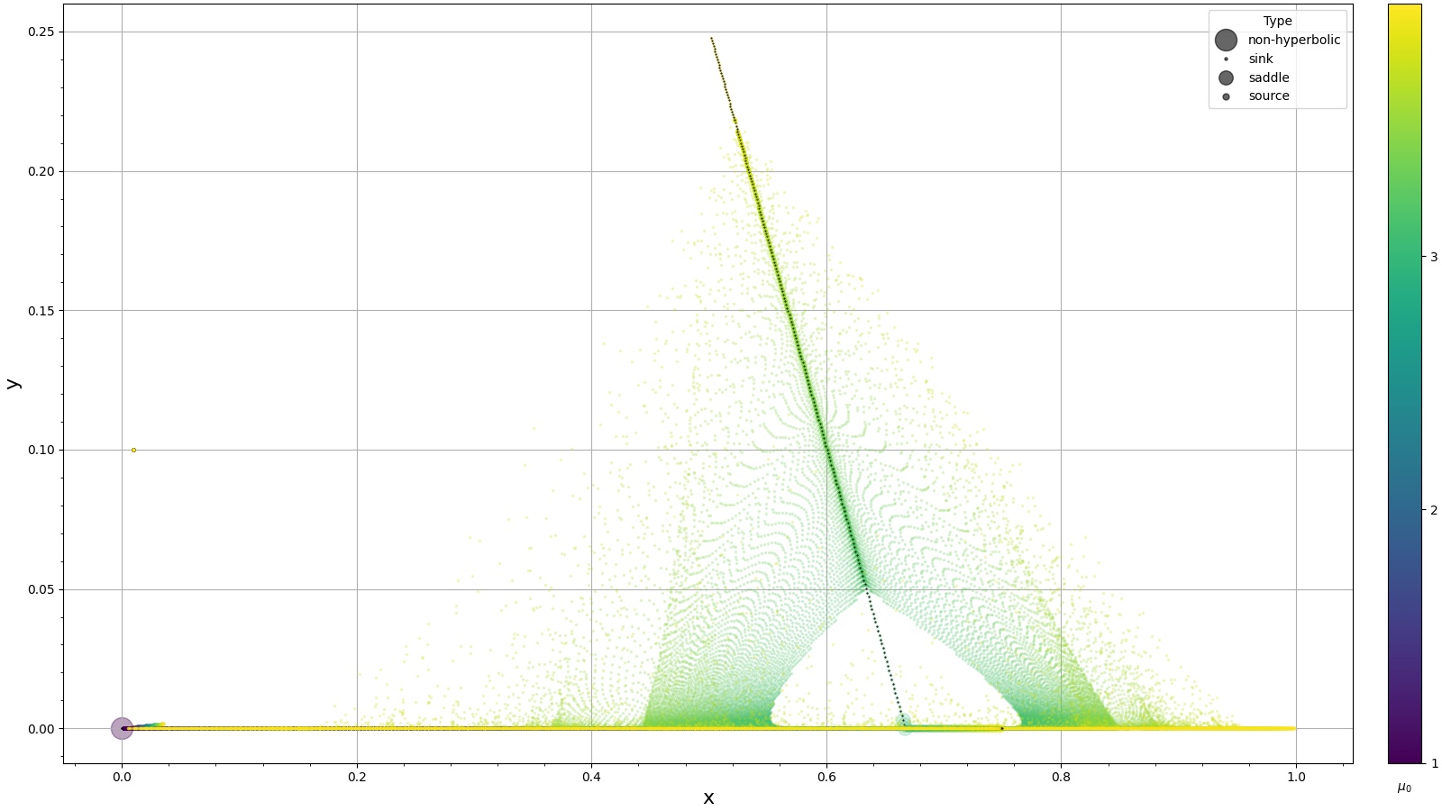
(a)

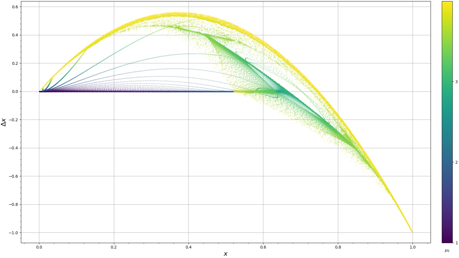
(b)

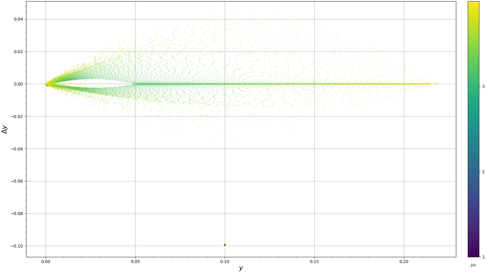
(c)

Figure 16: Analysis on phase portrait and phase space diagram about Extinction. No limit circles were found in this case.

3.5 Vorticella Strange

The last bifurcation type in our study is Vorticella Strange, which means that bifurcation diagram looks like a vorticella, only with more complicated internal structures. Figure 17(a) shows bifurcation diagram. When $\mu_{0}<2.0$, $x$ grows steadily without $y$. After presence of the predator, population of the prey starts to decrease. Both species show predictable population before $\mu_{0}=3.025$, at which we classify a Neimark-Sacker bifurcation as in Paraclete. Transient states occur between $3.025<\mu_{0}<3.200$, as indicated in the shaded region. Later, a $6$-cycle appears at $\mu_{0}=3.24$, which is also confirmed in Figure 18(b). The $6$-cycle becomes $3$-cycle at $\mu_{0}=3.40$, as shown in Figure 18(c), followed by chaos at $\mu_{0}=3.485$, which is also demonstrated in Figure 18(d). The system goes back to $6$-cycle around $\mu_{0}=3.540$, as we may also confirm in Figure 18(e). Afterwards, the system goes back to chaos, as shown in Figure 18(f).

Figure 17(b) shows Lyapunov spectrum of Voticella Strange. All four algorithms barely show positive spectra for both $x$ and $y$ before $\mu_{0}=3.5$. On the contrary, after$\mu_{0}=3.5$, four algorithms show positive Lyapunov exponents, where the system falls into chaos. For $\lambda_{x}$, Eckmann Y shows a decreasing tail below $\mu_{0}<1.5$, inconsistent from the other algorithms. Besides Equation showing two valleys between $1.500<\mu_{0}<2.304$ and $3.224<\mu_{0}<3.463$, the other three algorithms only provide flat spectra in the two regions.

Figure 19 shows analysis on eigenvalues of Vorticella Strange. At the first row, we see that both eigenvalues have zero imaginary parts, with absolute real parts of both greater than $1$ (see also first column in Figure 20). Thus, $E^{\prime}_{1}$ is a source. Similar analysis may also be done on $E^{\prime}_{2}$, as shown in the second row in Figure 19 as well as the second column in Figure 20. At $\mu_{0}=2.0$, it turns from a sink to a saddle, and it maintains as a saddle between $2.0<\mu_{0}<3.0$, after which it turns to a source. Finally, the third column in Figure 20 demonstrates that Neimark-Sacker bifurcation occurs at $\mu_{0}\approx 3.025$, with coordinates ($0.341,0.377$), as shown in Figure 21(a).

Similar bifurcation diagram was found by Hu et al.[10], and was identified as the Hopf bifurcation. However, the criteria for Hopf bifurcation in the two-dimensional system includes that the two eigenvalues are purely conjugate imaginary pair with zero real part[42]. Since Figure 19 shows that $\omega_{1}$ has a non-zero real part, our Vorticella Strange cannot be a Hopf bifurcation.

For the sake of integrity, phase portrait and phase space diagram of Vorticell Strange are also shown in Figure 21. Similar detailed meaning is discussed in the Section of Paraclete.

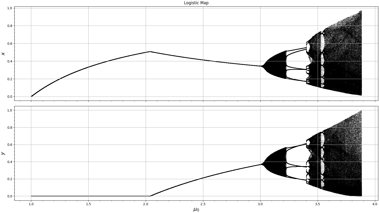
(a)

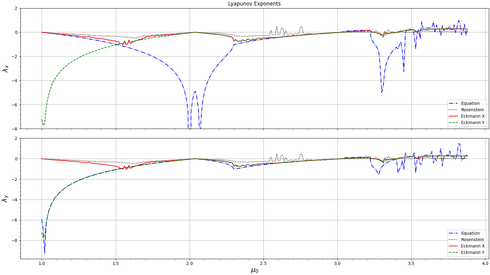
(b)

Figure 17: Bifurcation diagram and Lyapunov exponents of Vorticella Strange.

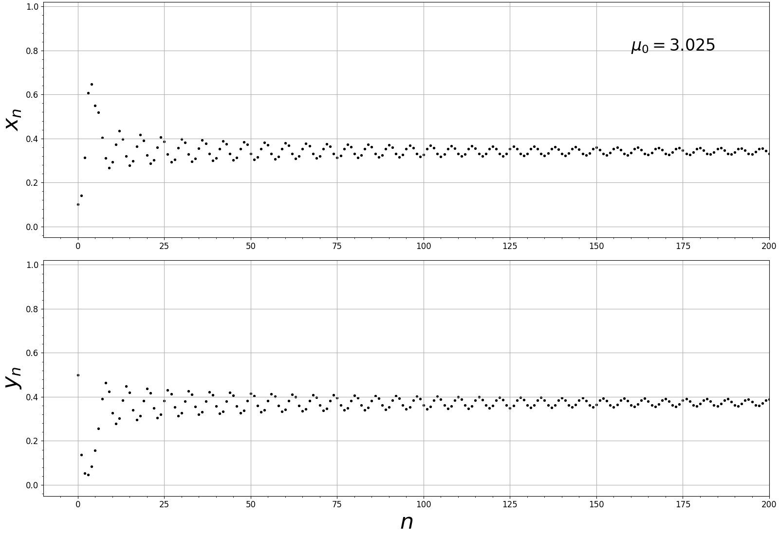
(a)

(b) fig:

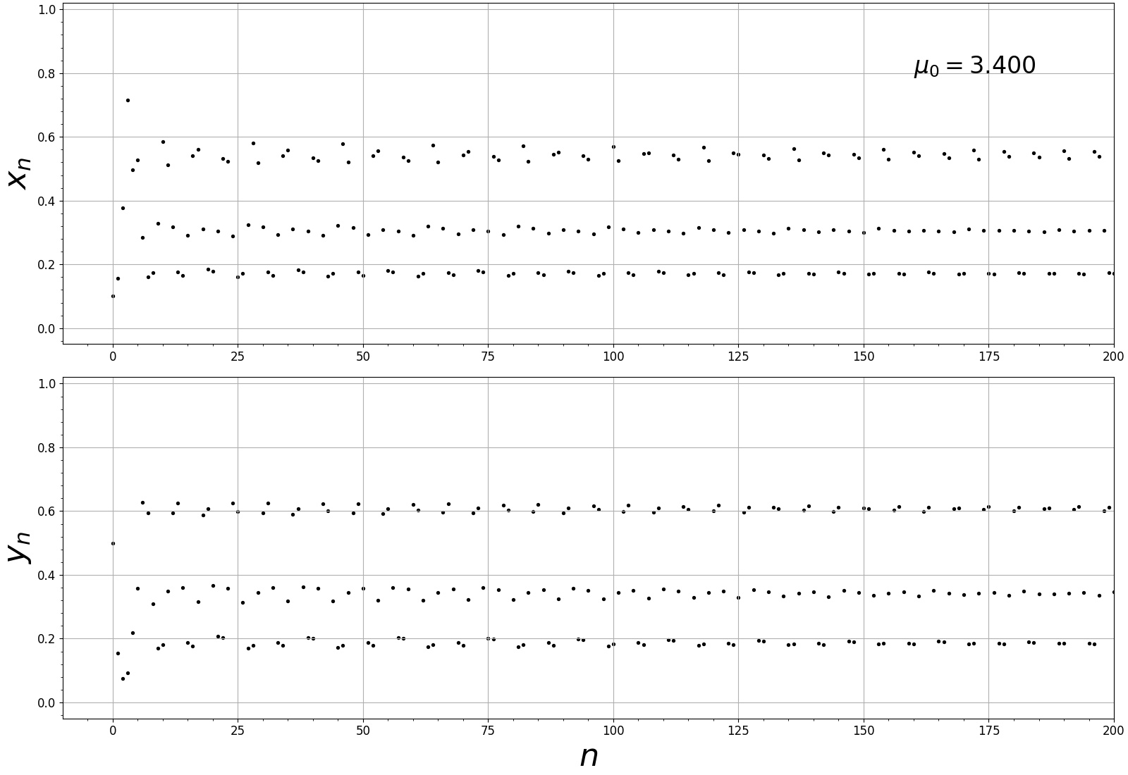
(c)

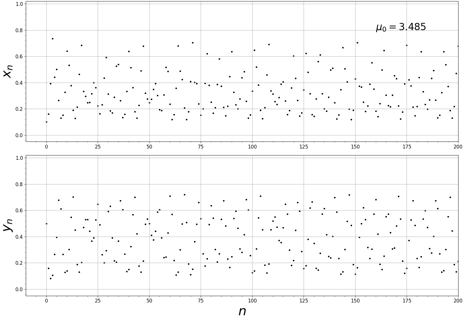
(d)

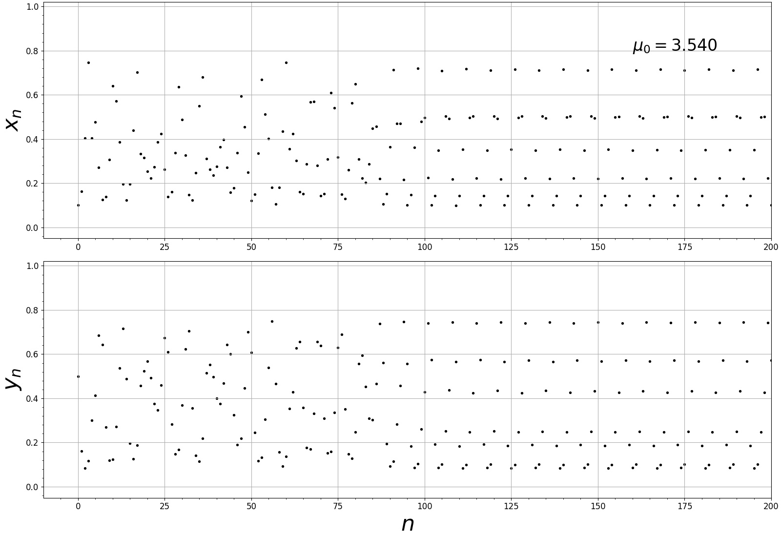
(e)

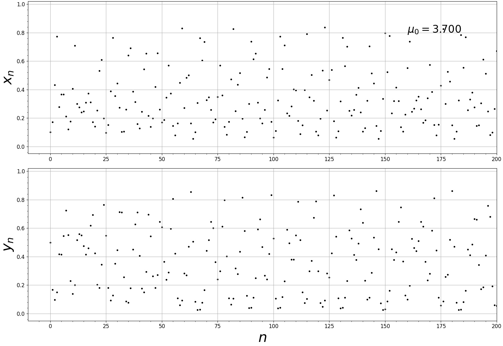
(f)

Figure 18: Population vs. iteration of Vorticella Strange.

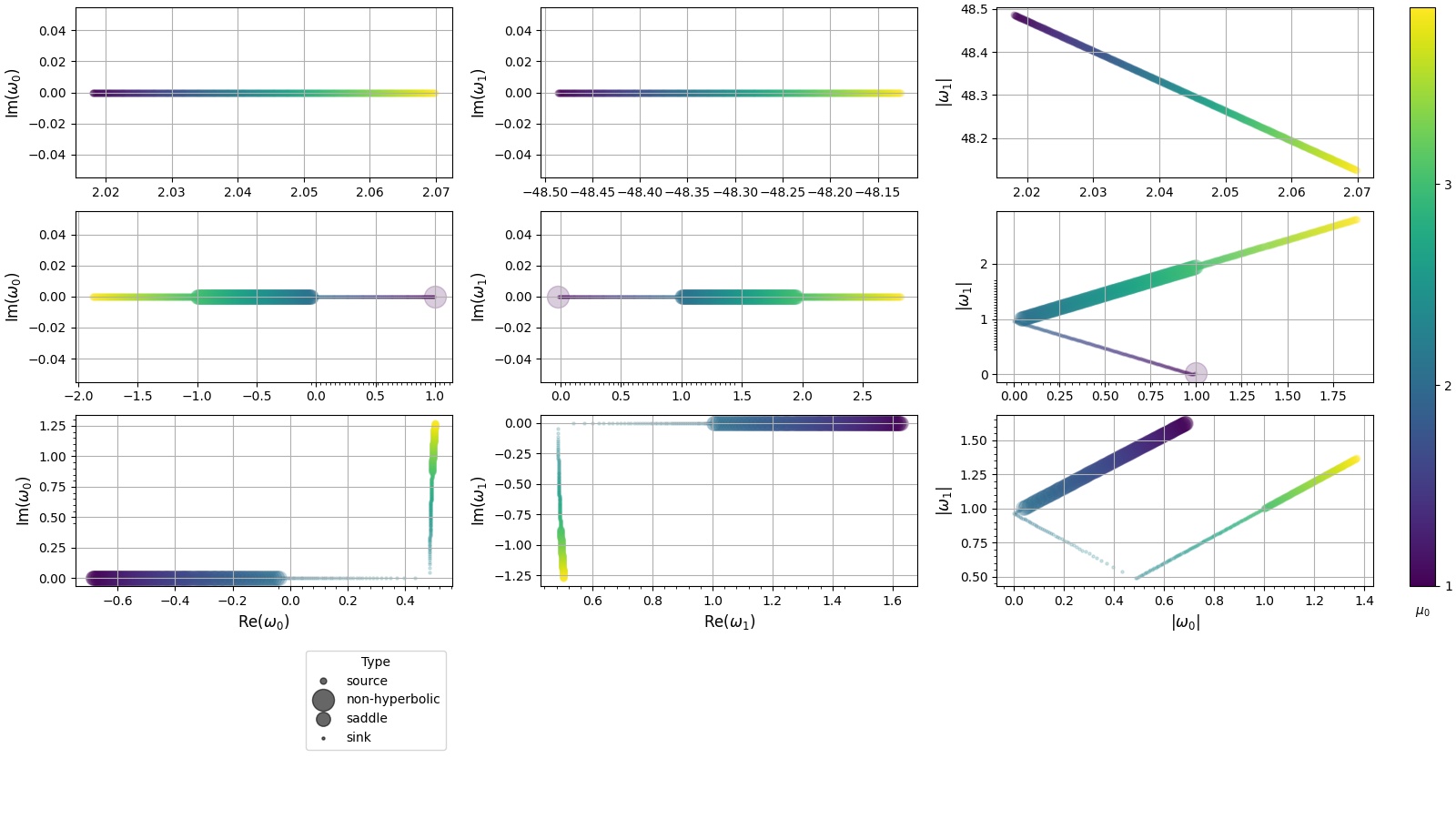
Figure 19: Analysis on eigenvalues for the case of Vorticella Strange. Legends have the same meaning described in Figure 4.

.

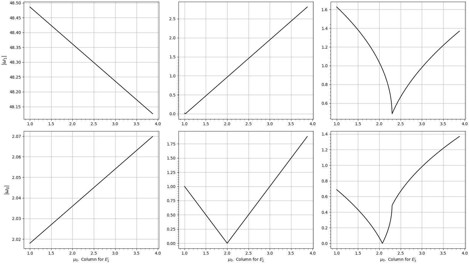
Figure 20: Absolute values of eigenvalues vs. growth rate at fixed points for Vorticella Strange. Important coordinates include: Upper middle panel ($3.025,1.935$). Upper-right corner panel ($2.299,0.491$), and ($3.035,1.000$). Lower-left corner panel ($2.069,0.000$), and ($2.370,0.490$).

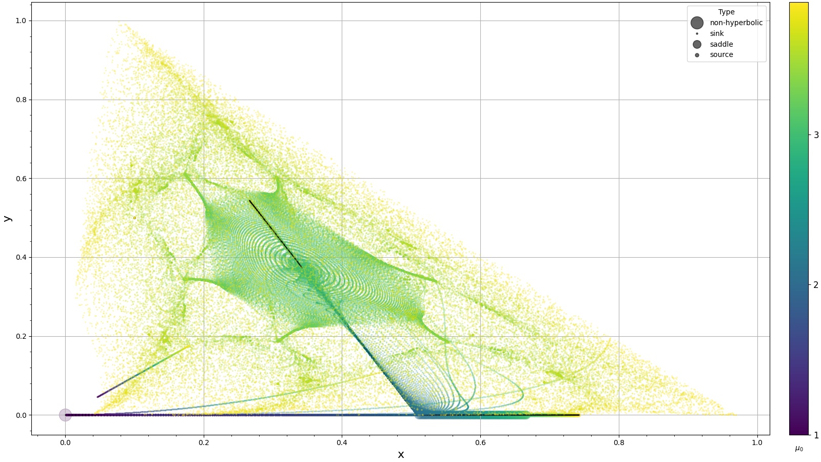
(a)

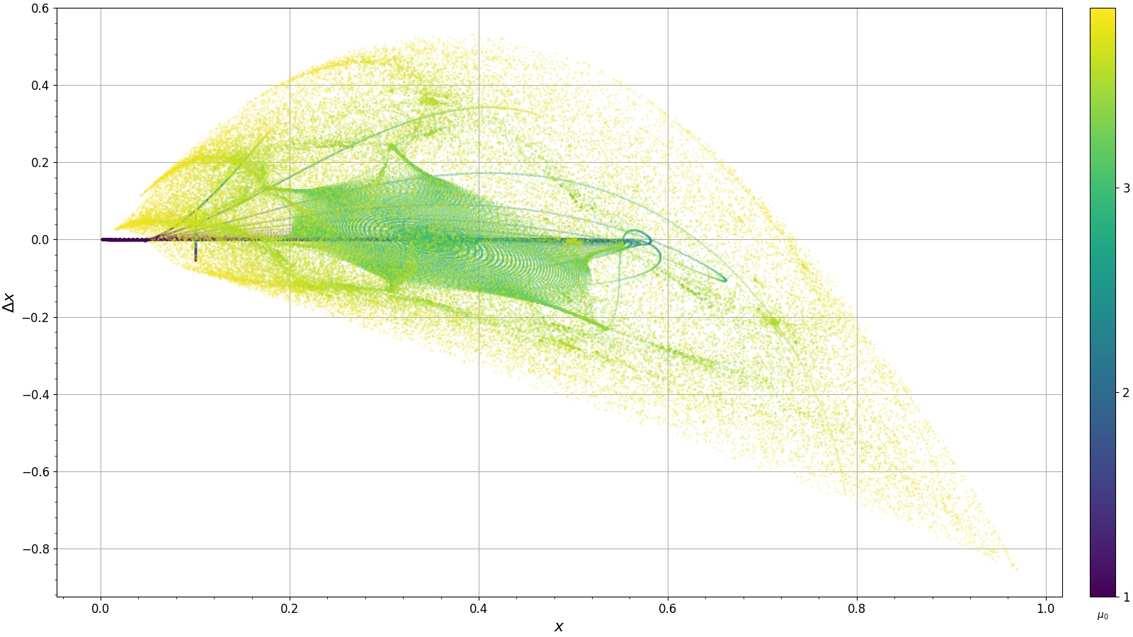
(b)

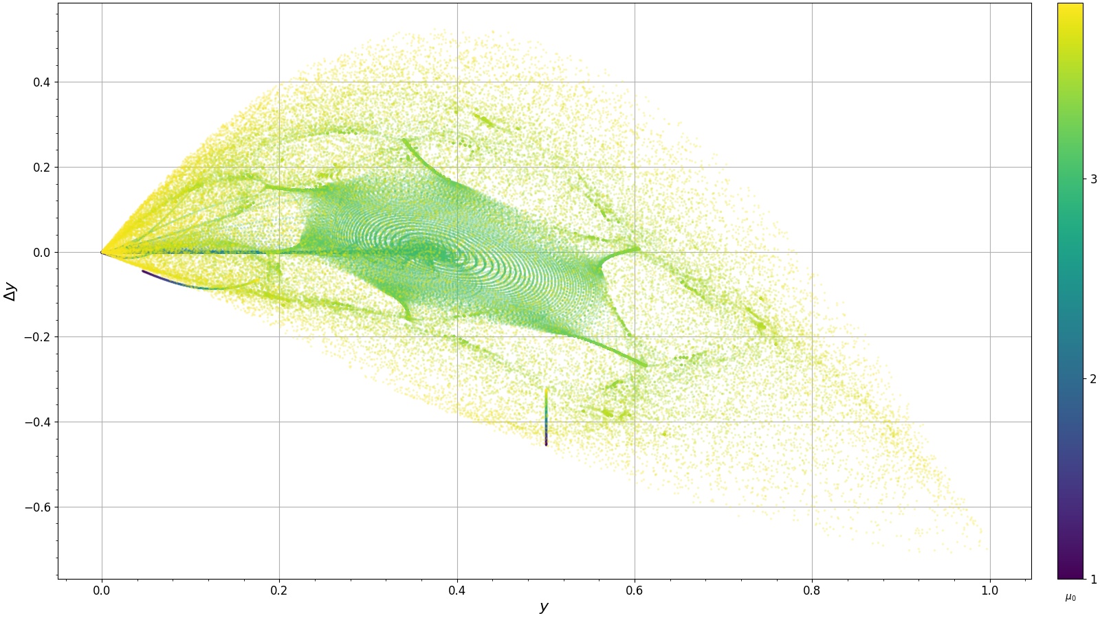
(c)

Figure 21: Analysis on phase portrait and phase space diagram about Vorticella Strange. (21(a))Phase portrait shows Neimark-Sacker bifurcation established at ($0.341,0.377$) with $\mu_{0}\approx 3.025$. See also caption in Figure 11.

4 Conclusions

We successfully built up a discrete-time model of two-dimensional mapping that resembles features of differential Lotka-Volterra Equations. We studied the topological types of fixed points, and found out that fascinating feather-like structures were formed around limit circles pierced through by the axis of fixed points in the phase portraits and phase space diagrams under various growth rates with Neimark-Sacker bifurcation. We further divided our dynamical systems into five categories by different shapes of bifurcation diagrams: Normal, Standard, Paraclete, Extinction, and Vorticella Strange. In every case, we studied the stability and topological types of the fixed points by criteria discussed in Lamma 1. In addition to plot the population vs. iteration, we also calculated Lyapunov exponents both by eigenvalues of Jacobian of mapping functions, and by Rosenstein algorithm and Eckmann et al. algorithm. Discrepancies clearly showed that Lyapunov exponents calculated by time-series algorithms may be unreliable within the range of chaos and at low growth rates, as well as when the Lyapunov exponents change dramatically. Furthermore, our model not only regained the $1$D logistic mapping of the prey under zero predator yet with non-zero initial predator population and with non-zero inter-species constants, but it also showed the normal competitiveness of the prey and the predator without chaos. The quintessence in the current research was that, besides the possibility for the prey and the predator to become chaotic altogether, it is also probable for the predator to go extinct at the chaotic state of the prey. In other words, human overpopulation would cause chaos in natural resources, ultimately in return erase the entire human race. Luckily, even under this difficult circumstance slim chance is still left upon us to continue our race under some specific growth rate, as we may see some isolated fixed points remain in the predator bifurcation diagram.

Our model may inspire conjecture on other relationships between two physical quantities, because mathematically what we demonstrated was that one quantity may dramatically reduce to zero at the state of chaos of the other. Therefore, it could be highly possible that, for example, the superconducting state, which refers to the zero resistance, may be achieved with chaos of some physical quantity that has relationship between resistance in the form of simultaneous difference equations.

5 Acknowledgment

We thank Pui Ching Middle School in Macau PRC for the kindness to support this research project.

References

- [1] Peter Roopnarine, Ecology and the Tragedy of the Commons, Sustainability 2013, 5(2), 749-773.
- [2] Ankit Kumar et al., A Computer-Based Simulation Showing Balance of the Population of Predator and Prey and the Effects of Human Intervention, 2021 IOP Conf. Ser.: Mater. Sci. Eng. 1031 012049
- [3] Cheng Sok Kin et al., Predicting Earth’s Carrying Capacity of Human Population as the Predator and the Natural Resources as the Prey in the Modified Lotka-Volterra Equations with Time-dependent Parameters, arXiv:1904.05002v2 [q-bio.PE]. Retrieved via https://doi.org/10.48550/arXiv.1904.05002
- [4] K.A. Hasan and M. F. Hama, ”Complex Dynamics Behaviors of a Discrete Prey-Predator Model with Beddington-DeAngelis Functional Response”, Int. J. Contemp. Math. Sciences, Vol. 7, 2012, no. 45, 2179 - 2195.
- [5] A George Maria Selvam et al, ”Bifurcation and Chaos Control for Prey Predator Model with Step Size in Discrete Time”, 2020 J. Phys.: Conf. Ser. 1543 012010.
- [6] Boshan Chen and Jiejie Chen, ”Bifurcation and Chaotic behavior of a discrete singular biological economic system.” Applied Mathematics and Computation, 219(2012) 2371-2386.
- [7] Yong Li et al, ”Flip and Neimark-Sacker Bifurcations of a Discrete Time Predator-Prey Model”, IEEE Access, Vol. 7, pp 123430-123435, 2019.
- [8] C. Wang and X. Li, J. Math. Ann. Appl., 422(2015) 920-939.
- [9] X.L. Liu and D.M. Xiau, Complex dynamic behaviors of a discrete-time predator-prey system, Chaos Solitons Fract., 32(2007)80-94.
- [10] Z. Hu, Z. Teng, and L. Zhang, Stability and bifurcation analysis of a discrete predator-prey model with nonmonotonic functional response, Nonlinear Anal. Real World Appl. 12(4)(2011)2356-2377.
- [11] Massimo Cencini, Fabio Cecconi, and Angelo Vulpiani, Chaos: From Simple Models To Complex Systems (Advances in Statistical Mechanics), Wspc; Illustrated edition (September 1, 2009)
- [12] J A Vano, J C Wildenberg, M B Anderson, J K Noel and J C Sprott, Chaos in low-dimensional Lotka–Volterra models of competition, Nonlinearity 19 (2006) 2391–2404.
- [13] Rubin H. Landau, Manuel J. Páez, and Cristian C. Bordeianu, Computational Physics, 2015 WILEY_VCH, pp. 356-357.
- [14] C.M. Evans and G.L. Findley, ”A new transformation for the Lotka-Volterra problem”, Journal of Mathematical Chemistry 25 (1999) 105-110.
- [15] Dunbar, S. R. (1983). Traveling wave solutions of diffusive Lotka-Volterra equations. Journal of Mathematical Biology, 17(1), 11-32.
- [16] Das, S. and Gupta, P. K. (2011). A mathematical model on fractional Lotka–Volterra equations. Journal of Theoretical Biology, 277(1), 1-6.
- [17] T. Bessoir and A. Wolf, Chaos Simulations, Physics Academic Software, North Carolina State University, Raleigh, NC 27695-8202, USA.
- [18] Pelinovsky, E., Kurkin, A., Kurkina, O., Kokoulina, M., and Epifanova, A. (2020). Logistic equation and COVID-19. Chaos, Solitons & Fractals, 140, 110241.
- [19] A. Mareno, L. Q. English, ”Flip and Neimark–Sacker Bifurcations in a Coupled Logistic Map System”, Discrete Dynamics in Nature and Society, vol. 2020, Article ID 4103606, 14 pages, 2020. https://doi.org/10.1155/2020/4103606
- [20] Bo Li, Qizhi He and Ruoyu Chen,”Neimark–Sacker bifurcation and the generate cases of Kopel oligopoly model with different adjustment speed”, Advances in Difference Equations (2020) 2020:72, https://doi.org/10.1186/s13662-020-02545-9.
- [21] Zeraoulia Elhadj and J. C. Sprott, ”The effect of modulating a parameter in the logistic map”, Chaos 18, 023119 (2008).
- [22] Andrey L. Shilnikov and Nikolai F. Rulkov, Origin of Chaos in a Two-Dimensional Map Modeling Spiking-Bursting Neural Activity, International Journal of Bifurcation and Chaos, Vol. 13, No. 11(2003), 3325-3340.
- [23] Waqas Ishaque, Qamar Din, Muhammad Taj and Muhammad Asad Iqbal,”Bifurcation and chaos control in a discrete-time predator–prey model with nonlinear saturated incidence rate and parasite interaction”, Advances in Difference Equations (2019) 2019:28, https://doi.org/10.1186/s13662-019-1973-z
- [24] Asifa Tassaddiq, Muhammad Sajjad Shabbir, Qamar Din and Humera Naaz, ”Discretization, Bifurcation and Control for a Class of Predator–Prey Interactions”, Fractal Fract. 2022, 6(1), 31; https://doi.org/10.3390/fractalfract6010031
- [25] Abd-Elalim Elsadany, H.A. EL-Metwally, E.M. Elabbasy, and H.N. Agiza, Chaos and bifurcation of a nonlinear discrete prey-predator system, Computational Ecology and Software, 2012, 2(3): 169-198.
- [26] Michael P. Hassell, Hugh N. Comins & Robert M. Mayt, ”Spatial structure and chaos in insect population dynamics”, Nature volume 353, pages 255–258 (1991)
- [27] A. A. Berryman and J.A. Millstein, ”Are Ecological Systems Chaotic-And If Not, Why Not?”, Trends Ecol Evol. 1989 Jan;4(1):26-8. doi: 10.1016/0169-5347(89)90014-1.
- [28] M. T. Rosenstein, J. J. Collins, and C. J. De Luca, “A practical method for calculating largest Lyapunov exponents from small data sets,” Physica D: Nonlinear Phenomena, vol. 65, pp. 117–134, 1993.
- [29] J. P. Eckmann, S. O. Kamphorst, D. Ruelle, and S. Ciliberto, “Liapunov exponents from time series,” Physical Review A, vol. 34, no. 6, pp. 4971–4979, 1986.
- [30] A.J. Lotka, ”Contribution to the Theory of Periodic Reaction”, J. Phys, Chem. 14(3), 271–274, 1910.
- [31] V. Volterra, ”Variazioni e fluttuazioni del numero d’individui in specie animali conviventi”. Mem. Acad. Lincei Roma. 2: 31–113, 1926.
- [32] Lotka-Volterra Equation Wikipedia, https://en.wikipedia.org/wiki/Lotka%E2%80%93Volterra_equations
- [33] Immanuel M. Bonze, Lotka-Volterra Equation and Replicator Dynamics: A Two-Dimensional Classification, Biol. Cybern 48, 201-221, 1983. Eq 4 in our work has the same form as Eq in this reference.
- [34] Steve H. Strogatz, Nonlinear Dynamics and Chaos, p.156, Addison Wesley, 2nd Ed.
- [35] Alan Wolf, Jack B. Swift, Harry L. Swinney and John A. Vastano, Determining Lyapunov Exponents from a Time Series, Physica 16D, 285-317, 1985.
- [36] Lorenzo Escot and Julio E. Sandubete Galan, ”A brief methodological note on chaos theory and its recent applications based on new computer resources”, Revista: ENERGEIA (ISSN: 1666-5732) Vol. VII, Núm. 1, 2020, pp 53-64.
- [37] Schölzel, Christopher. (2019, June 16). Nonlinear measures for dynamical systems (Version 0.5.2). Zenodo. http://doi.org/10.5281/zenodo.3814723
- [38] Codes and animations may be retrieved via https://github.com/weishanlee/LotkaVolterraChaos
- [39] Stephen T. Thornton and Jerry B. Marrion, Classical Dynamics of Particles and Systems, 5th Ed., CH4, ISBN-10:0534408966
- [40] IGI Global https://www.igi-global.com/dictionary/flip-bifurcation/11262
- [41] Herbert Goldstein, Charles Poole, John Safko, Classical Mechanics, 3rd Ed, CH11, ISBN-10:0321188977.
- [42] J. Hale, and H Koçak, Dynamics and Bifurcations. CH 11, Vol. 3, Berlin: Springer-Verlag (1991). ISBN-13: 9783540971412.