Thermal curvature perturbations in thermal inflation

Abstract

We compute the power spectrum of super-horizon curvature perturbations generated during a late period of thermal inflation, taking into account fluctuation-dissipation effects resulting from the scalar flaton field’s interactions with the ambient radiation bath. We find that, at the onset of thermal inflation, the flaton field may reach an equilibrium with the radiation bath even for relatively small coupling constants, maintaining a spectrum of thermal fluctuations until the critical temperature $T_{c}$, below which thermal effects stop holding the field at the false potential minimum. This enhances the field variance compared to purely quantum fluctuations, therefore increasing the average energy density during thermal inflation and damping the induced curvature perturbations. In particular, we find that this inhibits the later formation of primordial black holes, at least on scales that leave the horizon for $T>T_{c}$. The larger thermal field variance also reduces the duration of a period of fast-roll inflation below $T_{c}$, as the field rolls to the true potential minimum, which should also affect the generation of (large) curvature perturbations on even smaller scales.

1 Introduction

It is widely believed that the universe went through a period of inflation in its early stages [1, 2, 3, 4], thus explaining its observed homogeneity and isotropy on large scales, as well as its apparently small spatial curvature. Most importantly, inflation in principle provided the seeds for the small curvature perturbations that grew into the large-scale structure that we observe in the Universe.

Although the simplest models postulate a single period of slow-roll inflation lasting for at least 50-60 e-folds after the largest presently observable scales became super-horizon, there is a priori no reason to exclude scenarios with multiple inflation periods with different dynamics. In particular, it is well known that reheating after inflation may lead to the production of e.g. topological defects if the associated reheating temperature exceeds the grand unification scale ($\sim 10^{16}$ GeV) [5] or other unwanted relics such as moduli or gravitinos in supersymmetric (SUSY) models [6, 7, 8]. Such relics could have overclosed the Universe or spoiled the successful predictions of primordial nucleosynthesis through their late decay [9]. This and the fact that currently there is no evidence for such relics motivates considering scenarios with additional inflationary stages that could have diluted their abundances [10, 11, 12, 13, 14].

One of the most appealing possibilities is a late period of thermal inflation, where a scalar flaton field is trapped in a false vacuum by thermal effects above a certain critical temperature. Candidates to drive such a secondary inflation period are ubiquitous in SUSY and supergravity theories, in particular given the many flat directions in the scalar potential that characterize such models at the renormalizable level [15]. The spectrum of curvature perturbations generated during such a period (or possibly multiple periods) need not be nearly as scale-invariant as the one generated by the first period of slow-roll inflation, during which the large-scale perturbations observable in the Cosmic Microwave Background (CMB) anisotropies became super-horizon. In fact, this spectrum was recently computed in [16], where it was shown that large curvature perturbations could have been generated (on small scales) during a period of thermal inflation and a fast roll inflation period [17] that potentially followed it once thermal effects stopped trapping the field in the false vacuum state. These large curvature/density perturbations could have then collapsed into a significant population of primordial black holes upon horizon-reentry later in the radiation-dominated epoch. Such a possibility has attracted a substantial interest in the recent literature given the latter’s appeal as dark matter candidates and the possibility that these may explain the recent LIGO/Virgo detections of heavy black hole binaries (see e.g. [18]).

The analysis in [16] considered, however, only the part of the curvature spectrum generated by quantum fluctuations of the flaton scalar field. Since thermal effects are a crucial aspect in the dynamics of thermal inflation, one should investigate whether thermal fluctuations also play an important role, which is our goal with this work. We note, in particular, that the flaton field is trapped in a false vacuum at temperatures above a certain critical temperature, as we review in the next section, due to the large thermal mass resulting from its interactions with the ambient thermal bath. It is well-known that such interactions also lead to fluctuation-dissipation effects, resulting in an effective Langevin-like equation describing the dynamics of the scalar field. Such effects have been thoroughly analyzed in the context of warm inflation scenarios [19, 20, 21, 22, 23, 24, 25, 26, 27, 28, 29, 30, 31, 32, 33, 34, 35, 36], in setting initial conditions for slow-roll inflation in a pre-inflationary radiation epoch [37], and in cosmological phase transitions both after and during (warm) inflation [38, 39]. Our objective is then to apply the techniques developed in these contexts to the case of thermal inflation, and investigate their role in the generation of curvature perturbations during this period.

Surprisingly, we find that for thermal flaton fluctuations the amplitude of the curvature power spectrum is suppressed with respect to the purely quantum case analyzed in [16], at least for scales exiting the horizon before the temperature decreases below the critical value. This is essentially due to the fact that, as we will show, thermal effects, by enhancing flaton density fluctuations, also increase the time-dependent part of the average energy density during thermal inflation. This effect overcomes the enhancement of individual perturbation modes, therefore suppressing the corresponding power spectrum.

This work is organized as follows. We will start by constructing a generic model for thermal inflation in Section 2. The curvature perturbation spectrum induced by the thermal flaton fluctuations is computed in Section 3. In Section 4 we compare our result with the purely quantum computation performed in [16], discussing and summarizing our conclusions in Section 5. We use natural units throughout this work, $\hbar=c=k_{B}=1$ and the reduced Planck mass $M_{P}=2.435\times 10^{18}$ $\mathrm{GeV}$.

2 Thermal inflation

Let us consider a scalar field $\phi$ interacting with a thermal radiation bath at temperature $T$, with energy density $\rho_{R}=\frac{\pi^{2}}{30}g_{*}T^{4}$, where $g_{*}$ denotes the number of relativistic degrees of freedom. For concreteness, we consider a radiation bath made up of $N_{F}$ Dirac fermion species $\psi_{i}$, which interact with the scalar field through Yukawa interactions with universal coupling constant $g$:

$$\mathcal{L}_{Y}=-g\phi\sum_{i=1}^{N_{F}}\bar{\psi}_{i}\psi_{i}~{}.$$ (2.1)

We take the mass of the fermions $m_{\psi_{i}}\ll T$, so that they can be treated as relativistic degrees of freedom, but such that $m_{\psi_{i}}>H$ so that flat quantum field theory calculations for the decay width of scalars into fermions are valid [37].

We assume that the scalar field $\phi$ corresponds to a renormalizable flat direction, or flaton field, common in several SUSY/supergravity scenarios [11, 12, 14, 40, 41], such that its potential is only lifted by soft terms such as a mass term from SUSY breaking, and non-renormalizable terms. We are interested in the case where the squared mass term is negative, such that the field acquires a large expectation value $M_{0}$ at zero temperature from the latter’s interplay with the non-renormalizable operators. The interaction with the radiation bath induces, however, a thermal mass correction such that the field’s effective mass is of the form [42]:

$$m_{\text{eff}}^{2}=\alpha^{2}T^{2}-m^{2}~{},$$ (2.2)

where $m$ corresponds to the zero temperature (tachyonic) mass and $\alpha$ is the effective coupling to the thermal bath. For the Yukawa interactions described above we have $\alpha^{2}=g^{2}N_{F}/6$ at one-loop order. This implies, in particular, that for temperatures above the critical value, $T_{c}\equiv m/\alpha$, the origin is a stable minimum of the scalar potential, whereas for lower temperatures the minimum is non-trivial and asymptotes to $M_{0}$ in the limit of vanishing temperature. The origin thus constitutes a false vacuum state, near which we may write the scalar potential as:

$$V(\phi)=\frac{1}{3}M_{0}^{2}m^{2}+\frac{1}{2}m_{\text{eff}}^{2}\phi^{2}+\cdots~{},$$ (2.3)

where for concreteness we have chosen the constant term such that, if the leading non-renormalizable term is $\sim\phi^{6}$ the cosmological constant vanishes at the minimum, $V(\phi=M_{0})=0$, although this is not crucial to our analysis. For typical flat directions, $M_{0}\gg m$, since the scale at which the non-renormalizable operators become relevant is generically large (around the grand unification or even the Planck scale).

If, after the first period of slow-roll inflation, the Universe is reheated to attain a temperature $T>T_{c}$, the flaton field will thus be driven to the false minimum at the origin by Hubble friction, where it is trapped and gives a contribution $V_{0}=M_{0}^{2}m^{2}/3$ to the vacuum energy. Since the temperature drops as the universe expands, i.e. $\rho_{R}\propto a^{-4}$, eventually this vacuum energy may become dominant, thus triggering a new period of inflation, with expansion rate $H\simeq mM_{0}/3M_{P}\lesssim m$. Thermal inflation thus begins when the temperature drops below:

$$T_{i}=\bigg{(}\frac{10}{g_{*}\pi^{2}}\bigg{)}^{\frac{1}{4}}\sqrt{M_{0}m}~{}.$$ (2.4)

Assuming that there is no significant entropy production during thermal inflation, as we confirm in Appendix A, the temperature of the radiation bath drops as $T\propto a^{-1}$ during thermal inflation, eventually reaching the critical value $T_{c}$ below which the minimum at the origin is destabilized. The nature of the phase transition (or smooth crossover) that ensues is model-dependent and irrelevant to our discussion (see e.g. [43]), since we are mostly interested in what happens for temperatures $T_{c}<T<T_{i}$.

We note that thermal inflation is only possible if the flaton field has a non-negligible interaction with the thermal bath, and in particular $T_{i}>T_{c}$ imposes:

$$\alpha>\bigg{(}\frac{g_{*}\pi^{2}}{10}\bigg{)}^{\frac{1}{4}}\sqrt{\frac{m}{M_{0}}}~{}.$$ (2.5)

For instance, for $m\sim 10$ TeV and $M_{0}\sim M_{P}$, this imposes the lower bound $\alpha\gtrsim 10^{-7}$ for $g_{*}=10-100$. Although this may not seem too restrictive, we note that the number of e-folds of thermal inflation is given by:

$$N_{e}^{\text{(TI)}}=\ln\bigg{(}\frac{T_{i}}{T_{c}}\bigg{)}=\frac{1}{2}\ln\bigg{(}\frac{M_{0}}{m}\bigg{)}+\frac{1}{4}\ln\bigg{(}\frac{10}{\pi^{2}g_{*}}\bigg{)}+\ln(\alpha)~{}.$$ (2.6)

For the reference values given above, we see that a period of thermal inflation lasting more than 10 e-folds is only possible for $\alpha\gtrsim 0.01$, with even larger effective couplings required for scenarios with a smaller hierarchy between the mass scales $m$ and $M_{0}$.

We note that inflation does not necessarily end when the temperature falls below $T_{c}$, since expansion only stops accelerating once the flaton’s kinetic energy surpasses its potential energy. Below $T_{c}$ the field develops a tachyonic instability, since $m_{\text{eff}}^{2}\simeq-m^{2}<0$ once $T\ll T_{c}$, and its value moves away from the origin as $\sim e^{mt}\sim e^{{\frac{m}{H}}N_{e}}$ for $H\lesssim m$, and there may be a period of fast-roll inflation [17] until the field gets close to the minimum at $M_{0}$ and its kinetic energy takes over. Note that, in the opposite regime $m\lesssim H$, thermal inflation would be followed by an additional period of slow-roll inflation, but we will not consider this regime in our discussion. The duration of the fast-roll period is, of course, model dependent and, moreover, dependent on the mean field value at the critical temperature.

In [16, 17] it was shown that this period may last for as much as, or even longer than, the thermal inflation period for $H/m\lesssim 1$, depending on the flaton’s mass value. This assumed, however, that the mean field value at the critical temperature is set by quantum fluctuations, which as we will see is not necessarily the case. In particular, thermal fluctuations typically enhance the field’s variance at $T_{c}$, therefore reducing the duration of the subsequent fast-roll period. For this reason, we will restrict our analysis to the thermal inflation period ($T_{c}<T<T_{i}$), discussing the implications of our results to the subsequent cosmological evolution at the end of our discussion.

Independently of whether or not there is a significant period of inflation below $T_{c}$, the field will eventually begin oscillating about the minimum of its potential and decay away through the Yukawa interactions in Eq. (2.1) [44]. Although we do not specify the exact nature of the fermion fields in the thermal bath, since we are only modelling the interactions between the flaton and the ambient radiation and our discussion is largely independent of the particular interactions considered, it is implicit that such interactions will eventually lead to the reheating of the Standard Model degrees of freedom at temperatures exceeding at least a few MeV to ensure the correct conditions for primordial nucleosynthesis.

We note that having late thermal inflation and fast-roll inflation periods alters the predictions of inflationary cosmology [45], since the largest CMB scales leave the horizon 50-60 e-folds before the end of the full inflationary epoch, including the primary slow-roll inflation period, which therefore must necessarily be shorter.

Although the leading effect of the interactions between the flaton and the thermal bath is the thermal mass correction responsible for its trapping at the origin, it also induces fluctuation-dissipation effects in the flaton’s dynamics that, as we will see, can play an important role in the evolution of field perturbations during thermal inflation. These have been considered in [46] to analyze the nature of the phase transition at $T_{c}$, but their effects on the associated spectrum of curvature perturbations have so far been overlooked. To study them, we consider the full Langevin-like equation for the flaton field modes $\phi_{k}$ of comoving momentum $k$, which can be obtained through standard techniques in linear response theory assuming the ambient radiation bath is close to an equilibrium state, and is given by (see e.g. [25, 47]):

$$\ddot{\phi}_{k}+(3H+\Gamma_{\phi})\dot{\phi}_{k}+\omega_{k}^{2}\phi_{k}=\xi_{k}~{},$$ (2.7)

where $\omega_{k}^{2}=k^{2}/a^{2}+m_{\text{eff}}^{2}$ and $\Gamma_{\phi}$ is the dissipation coefficient, which for a field oscillating near a local minimum of its potential (in this case the false minimum at the origin for $T>T_{c}$) coincides with its finite-temperature decay width [48]. On the right hand side of (2.7), $\xi_{k}$ is a stochastic noise term which encodes the randomness of the field’s interactions with the thermal bath. For modes with physical momentum $p=k/a\lesssim\pi T$ it is well approximated by a gaussian white noise term with a two-point correlator given by the fluctuation-dissipation relation [46, 49].:

$$\braket{\xi_{k}(t)\xi_{{k}^{\prime}}(t^{\prime})}=2\Gamma_{\phi}T\frac{(2\pi)^{3}}{a^{3}}\delta^{3}(\bm{k}+\bm{k}^{\prime})\delta(t-t^{\prime})~{}.$$ (2.8)

We note that physically this is reminiscent of the Brownian motion of a heavy particle in an gas, for which random collisions with the gas molecules induce an effective friction that damps its motion. However, the particle never actually comes to rest due to the very same random collisions, eventually reaching an equilibrium with the gas. We expect something very similar to occur to the flaton field modes, with the combined effects of dissipation ($\Gamma_{\phi}$) and thermal fluctuations ($\xi_{k}$) driving the field towards a thermal equilibrium with the radiation bath. This behaviour has been observed for scalar fields interacting with a radiation bath both in an inflationary and non-inflationary context [37, 39], so we anticipate that the same will occur in the case of thermal inflation.

At finite temperature the flaton decay width into relativistic fermions is given by [27, 37]:

$$\Gamma_{\phi}(p)=\frac{3m_{\text{eff}}^{2}\alpha^{2}}{4\pi\omega_{p}}\bigg{\{}1+\frac{2T}{p}\ln\bigg{[}\frac{1+\exp(-\frac{\omega_{+}}{T})}{1+\exp(-\frac{\omega_{-}}{T})}\bigg{]}\bigg{\}}~{},$$ (2.9)

where $\omega_{\pm}=\frac{|\omega_{p}\pm p|}{2}$ and we have neglected the mass of the fermions, $T\gg m_{\psi_{i}}$. Note that fermions acquire a mass through their interaction with the flaton field but, as we will obtain bellow, $\sqrt{\braket{\phi^{2}}}\lesssim T$ for perturbative couplings.

Since the thermal bath will excite field modes $p\lesssim T$ and $m_{\text{eff}}\lesssim T$, the decay width can be well approximated by:

$$\Gamma_{\phi}\simeq\frac{3m_{\text{eff}}^{2}\alpha^{2}}{16\pi T}\simeq{\frac{3\alpha^{4}}{16\pi}}T~{},$$ (2.10)

where in the last step we have used $m_{\text{eff}}\simeq\alpha T$ for $T\gtrsim T_{c}$. At the onset of thermal inflation, we then have:

$$\left.{\Gamma_{\phi}\over H}\right|_{T_{i}} \simeq {9\over 16\pi}\left({10\over g_{*}\pi^{2}}~{},\right)^{1/4}\alpha^{4}{M_{P}\over\sqrt{M_{0}m}}$$ (2.11)

$$\simeq 2.3g_{*}^{-1/4}\left({\alpha\over 0.03}\right)^{4}\left({M_{P}\over M_{0}}\right)^{1/2}\left(m\over 10\ \mathrm{TeV}\right)^{-1/2}~{},$$

so that we expect dissipative effects to play an important role in the field’s dynamics roughly for the same range of the effective coupling $\alpha$ leading to a period of thermal inflation lasting for more than 10 e-folds, as we have seen above. In the next section we compute the thermal field correlators and associated curvature perturbation power spectrum to better quantify this statement.

3 Curvature Perturbations

Let us consider the gauge-invariant curvature perturbation on uniform density hypersurfaces, which in the flat gauge can be written as [50, 51]:

$$\zeta=-\frac{H}{\dot{\braket{\rho}}}\delta\rho~{},$$ (3.1)

where the perturbation of a generic function is given by $\delta f(t,\bm{x})\equiv f(t,\bm{x})-\braket{f(t,\bm{x})}$, and brackets denote its thermal averaged value. The dimensionless power spectrum of $\zeta$ is defined as [16],

$$\Delta^{2}_{\zeta}(k) =\frac{k^{3}}{2\pi^{2}}\int d^{3}x\;\exp(-i\bm{k}\cdot\bm{x})\braket{\zeta(0)\zeta(\bm{x})}~{},$$ (3.2)

$$=\frac{2k^{3}}{(2\pi)^{2}}\bigg{(}\frac{H}{\dot{\braket{\rho}}}\bigg{)}^{2}\int d^{3}x\;\exp(-i\bm{k}\cdot\bm{x})\braket{\delta\rho(0)\delta\rho(\bm{x})}~{}.$$

The total energy density $\rho$ during thermal inflation includes the contributions from both the flaton field and the radiation fluid [52]:

$$\rho=\rho_{\phi}+\rho_{R}=\frac{1}{2}\dot{\phi}^{2}+V(\phi)+\frac{1}{2}a^{-2}(t)\partial_{i}\phi\partial_{i}\phi+\frac{\pi^{2}}{30}g_{*}T^{4}~{},$$ (3.3)

and so we have

$$\braket{\rho} =\frac{\pi^{2}}{30}g_{*}T^{4}+\frac{1}{3}m^{2}M_{0}^{2}+\frac{1}{2}m_{\text{eff}}^{2}\braket{\phi^{2}}+\frac{1}{2}\braket{\dot{\phi}^{2}}+\frac{1}{2}a^{-2}\braket{\partial_{i}\phi\partial_{i}\phi}~{},$$ (3.4a)

$$\delta\rho =\frac{1}{2}m_{\text{eff}}^{2}\delta(\phi^{2})+\frac{1}{2}\delta(\dot{\phi}^{2})+\frac{1}{2}a^{-2}\delta(\partial_{i}\phi\partial_{i}\phi)~{}.$$ (3.4b)

Since density perturbations involve perturbations of quadratic functions of the field and its derivatives, the power spectrum, Eq. (3.2), involves contributions of the form:

$$\braket{\delta(X_{i}(0)^{2})\delta(X_{j}(\bm{x})^{2})}=\braket{X_{i}(0)^{2}X_{j}(\bm{x})^{2}}-\braket{X_{i}(0)^{2}}\braket{X_{j}(\bm{x})^{2}}~{},$$ (3.5)

where $X_{i}$ generically denotes the field perturbations and their derivatives. The first term on the right-hand side corresponds to 4th moments involving the gaussian variables $X_{i}$. According to Isserlis’ theorem [53] it is possible to write a $k$th moment of zero-average gaussian variables in terms of their variances. Thus, the correlators can be simply written as [54]:

$$\braket{\delta(X_{i}(0)^{2})\delta(X_{j}(\bm{x})^{2})}=2\braket{X_{i}(0)X_{j}(\bm{x})}^{2}~{}.$$ (3.6)

The two-point correlation function for the energy density is then:

$$\braket{\delta\rho(0)\delta\rho(\bm{x})} =\frac{m_{\text{eff}}^{4}}{2}\braket{\phi(0)\phi(\bm{x})}^{2}+m_{\text{eff}}^{2}\braket{\phi(0)\dot{\phi}(\bm{x})}^{2}+a^{-2}m_{\text{eff}}^{2}\braket{\phi(0)\partial_{i}\phi(\bm{x})}^{2}~{},$$ (3.7)

$$\quad+\frac{1}{2}\braket{\dot{\phi}(0)\dot{\phi}(\bm{x})}^{2}+a^{-2}\braket{\dot{\phi}(0)\partial_{i}\phi(\bm{x})}^{2}+\frac{a^{-4}}{2}\braket{\partial_{i}\phi(0)\partial_{j}\phi(\bm{x})}^{2}~{},$$

that is, contributions from all possible correlation functions involving $\phi$, $\dot{\phi}$ and $\partial_{i}\phi$.

We note that we are interested in computing the curvature perturbation power spectrum on super-horizon scales, $k\ll aH$. To do this we need to compute the field variance $\langle\phi^{2}\rangle$ and the average kinetic and gradient energies appearing in Eq. (3.4a), which involve integrating over all thermally excited field modes. Since the noise term correlator is exponentially suppressed for physical momentum scales $p\gtrsim\pi T$ [46], we use this value as a hard cutoff. This can be translated into a comoving momentum cutoff $k_{c}=\pi T_{c}$ if we set $a(T_{c})=1$, following the conventions of [16] to allow for a better comparison with the purely quantum calculation.

To compute the power spectrum we need the three combinations of the correlations between $\phi_{k}$ and $\dot{\phi}_{k}$, i.e. $\braket{\phi_{k}\phi_{k}}$, $\braket{\phi_{k}\dot{\phi}_{k}}$ and $\braket{\dot{\phi}_{k}\dot{\phi}_{k}}$. These are the building blocks of all the remaining correlation functions involved in the power spectrum. We will explicitly compute the correlator of the field modes and list all others in Appendix B as their computation follows similar steps.

The equal-time two-point correlation function of the field modes can be written in terms of the Green’s function associated with (2.7) and the noise correlator:

$$\braket{\phi_{k}(z)\phi_{k^{\prime}}(z)}=H^{-4}\int_{z_{i}}^{z}ds_{1}\;\int_{z_{i}}^{z}ds_{2}\;s_{1}^{-2}s_{2}^{-2}G_{s}(z,s_{1})G_{s}(z,s_{2})\braket{\xi_{k}(s_{1})\xi_{k^{\prime}}(s_{2})}~{},$$ (3.8)

where we have traded the time-dependence for a dependence on the variable $z=T/H$, with $z_{i}=T_{i}/H$. Note that $z\propto a^{-1}$ during thermal inflation, so that it is a decreasing function of time. We have ignored the contributions from the homogeneous solutions of (2.7) since, as we will see bellow, they quickly become subdominant. These are required, however, to compute the Green’s function, which is given by the usual expression:

$$G_{s}(z,s)=\frac{\phi_{k}^{(1)}(s)\phi_{k}^{(2)}(z)-\phi_{k}^{(1)}(z)\phi_{k}^{(2)}(s)}{W(\phi_{k}^{(1)},\phi_{k}^{(2)})(s)}~{},\\$$ (3.9)

where $\phi_{k}^{(1)}$ and $\phi_{k}^{(2)}$ are the homogeneous solutions of equation (2.7) and $W$ denotes their Wronskian.

During most of thermal inflation, except for temperatures close to the critical value, the thermal mass dominates over the field’s zero temperature mass, $\alpha T\gg m$. This allows us to compute analytically the field modes, and thus obtain the field’s two-point correlation function with a decay width of the form (2.10).

The homogeneous equation of motion for the flaton field modes (2.7) can be written in terms of the $z$ variable as:

$$z^{2}\phi_{k}^{\prime\prime}-z\left(2+\gamma z\right)\phi_{k}^{\prime}+z^{2}\bar{\omega}_{k}^{2}\phi_{k}=0~{},$$ (3.10)

where $\bar{\omega}_{k}^{2}\equiv\omega_{k}^{2}/T^{2}\simeq k^{2}/T_{c}^{2}+\alpha^{2}$ and $\gamma\equiv 3\alpha^{4}/16\pi$, such that $\Gamma_{\phi}/H=\gamma z$. Let us define $\phi_{k}=ze^{\gamma z/2}\chi_{k}$, such that:

$$\chi_{k}^{\prime\prime}+\left(\bar{\omega}_{k}^{2}-{\gamma^{2}\over 4}-{\gamma\over z}-{2\over z^{2}}\right)\chi_{k}=0~{}.$$ (3.11)

Even though we can express the exact solutions of the above equation in terms of Whittaker functions [55], it is more instructive to note that, since $\gamma\ll\bar{\omega}_{k}^{2}$ for $\alpha\lesssim 1$ and $z>z_{c}=m/\alpha H>\alpha^{-1}>1$, we may neglect all the terms inside the brackets in Eq. (3.11) except for the one involving $\bar{\omega}_{k}^{2}$ to a good approximation. This means that the homogeneous solutions are approximately given by:

$$\phi_{k}^{(1)}(z)\simeq ze^{{\gamma\over 2}z}\sin(\bar{\omega}_{k}z)~{},\qquad\phi_{k}^{(2)}(z)\simeq ze^{{\gamma\over 2}z}\cos(\bar{\omega}_{k}z)~{},$$ (3.12)

thus constituting oscillatory functions in the $z$ variable with an amplitude decreasing due to both Hubble expansion ($z\propto a^{-1}$) and the field’s decay into the light fermions. This yields the Green’s function:

$$G_{s}(z,s)={1\over\bar{\omega}_{k}}\frac{z}{s}\exp\bigg{[}{\gamma\over 2}(z-s)\bigg{]}\sin\bigg{[}\bar{\omega}_{k}(z-s)\bigg{]}~{}.$$ (3.13)

The noise correlation function can be written in terms of the $z$ variable as:

$$\braket{\xi_{k}(z_{1})\xi_{k^{\prime}}(z_{2})} =2Hz_{1}\Gamma_{\phi}T\frac{(2\pi)^{3}}{a^{3}}\delta^{3}(\bm{k}+\bm{k}^{\prime})\delta(z_{1}-z_{2})~{},$$ (3.14)

$$\simeq 2\gamma H^{3}z_{1}^{6}\frac{(2\pi)^{3}}{z_{c}^{3}}\delta^{3}(\bm{k}+\bm{k}^{\prime})\delta(z_{1}-z_{2})~{},$$

where in the second line we used the dominance of the thermal mass for $T>T_{c}$.

We may now substitute Eqs. (3.13) and (3.14) into Eq. (3.8) to obtain the field’s two-point correlation function:

$$\braket{\phi_{k}(z)\phi_{k^{\prime}}(z)}=(2\pi)^{3}\delta^{3}(\bm{k}+\bm{k}^{\prime})\frac{T}{a^{3}\omega_{k}^{2}}(1-\delta)~{},\qquad\delta=\exp\bigg{[}-\frac{3\alpha^{4}}{16\pi}\frac{T_{i}}{H}\bigg{(}1-\frac{T}{T_{i}}\bigg{)}\bigg{]}~{},$$ (3.15)

where again we used that $\bar{\omega}_{k}\gg\gamma$. Note that for $\Gamma_{\phi}/H(T_{i})\gtrsim 1$, we have $\delta\ll 1$ for all temperatures below $T_{i}$ (but above $T_{c})$, thus yielding a thermal equilibrium distribution for the field modes that is independent of the decay width. This means that if the field decays efficiently at the onset of thermal inflation it will attain an equilibrium distribution that simplify redshifts with expansion (with corresponding decrease in temperature). This is a generic result obtained in other cosmological contexts [37, 39] that we now recover also within thermal inflation – it simply states that if the field interacts significantly with the thermal bath at some point during its evolution it reaches a near-thermal configuration that is subsequently maintained unless there is some significant change in the field’s properties (in our case the tachyonic instability just below the critical temperature).

We note that the two-point correlation function vanishes at the onset of thermal inflation by construction, since the integral Eq. (3.8) is zero at $z=z_{i}$. This assumes that field modes were not excited when thermal inflation begins, which need not be the case since interactions with the thermal bath are present in the prior radiation-dominated epoch. If field modes thermalize before its vacuum energy becomes dominant, Eq. (3.15) will nevertheless hold (with $\delta\simeq 0$), since this result is also valid for a radiation-dominated cosmological background [37]. However, we note that during the radiation era $\Gamma_{\phi}/H\propto T/H\propto a$, while $\Gamma_{\phi}/H\propto a^{-1}$ during thermal inflation, so that this ratio attains its maximum value at the onset of thermal inflation. Recalling Eq. (2.11), we conclude that $\alpha\gtrsim 0.01$ is required for field thermalization if the zero temperature mass $m$ is not far from the TeV scale at which new physics may be expected. As discussed in the previous section, this is exactly the regime where a period of thermal inflation lasting more than 10 e-folds (and which can in particular sufficiently dilute unwanted relics of the first reheating process) can occur. We will thus henceforth focus our analysis on this parametric regime, in which the field thermalizes either before or at the onset of the thermal inflation epoch.

We may now use Eq. (3.15) to compute the field variance and related correlation functions, as we detail in Appendix B. We obtain for the total average energy density:

$$\braket{\rho}=\frac{\pi^{2}}{30}\left(g_{*}+\frac{5}{\pi}(1-\delta)\right)T^{4}+\frac{1}{3}m^{2}M_{0}^{2}~{},$$ (3.16)

where we note that the field contributes essentially as an additional bosonic degree of freedom to the radiation energy density if thermalization is efficient ($\delta\ll 1$). Its contribution is not exactly one degree of freedom since we have considered a hard-cutoff on the momentum of the modes that are excited by interactions with the thermal bath at $k_{c}=\pi T_{c}$. This is only an approximation to the smooth cutoff associated with the noise correlator [46], which nevertheless captures the essential physics of the problem.

Using the values of each component of the power spectrum (3.5) given in Appendix B, the density perturbations are:

$$\int d^{3}x\;\exp(-i\bm{k}\cdot\bm{x})\braket{\delta\rho(0)\delta\rho(\bm{x})}\approx\frac{\pi T^{5}}{6a^{3}}\bigg{[}1+3\bigg{(}\frac{3\alpha^{4}}{32\pi^{2}}\bigg{)}^{2}\bigg{(}1-\frac{\alpha}{\pi}\arctan\left({\pi\over\alpha}\right)\bigg{)}\bigg{]}(1-\delta)^{2}~{},$$ (3.17)

to leading order on super-horizon scales $k<aH<\alpha T_{c}$. We note that the first term within the square brackets dominates over the second one. This then yields for the power spectrum on super-horizon scales:

$${\Delta^{2}_{\zeta}}^{\text{(therm)}}(k) = \frac{150}{(2\pi)^{5}}\frac{k^{3}}{T_{c}^{3}}\frac{(1-\delta)^{2}}{\bigg{[}g_{*}+\frac{5}{\pi}(1-\delta)-\frac{5}{\pi}\frac{3\alpha^{4}}{64\pi}\frac{T}{H}\delta\bigg{]}^{2}}~{},$$ (3.18)

$$\simeq \frac{150}{(2\pi)^{5}}\frac{\alpha^{3}}{g_{*,f}^{2}}\bigg{(}\frac{H}{m}\bigg{)}^{3}\bigg{(}\frac{k}{k_{c}}\bigg{)}^{3}~{},$$

where in the second line we have taken the prompt thermalization limit, i.e. $\delta\ll 1$, in which case the flaton field contributes to the total number of relativistic degrees of freedom, given by $g_{*,f}\simeq g_{*}+5/\pi$. Note that this result is time-independent, reflecting the freeze-out of curvature perturbations on super-horizon scales and thus the single-fluid nature of the dynamics, i.e. the fact that the flaton field thermalized with the radiation bath.

The power spectrum is blue-tilted so its maximum value is attained for the last scale to leave the horizon during thermal inflation, i.e. $k_{c}=H$ which leaves at $T=T_{c}$. Although our calculation assumes the dominance of the thermal piece of the flaton’s mass, an approximation that breaks down close to the critical temperature, we may extrapolate our results with a reasonable accuracy to $k_{c}$, thus yielding an upper bound on the power spectrum of scales leaving the horizon before the phase transition, in the thermal equilibrium limit:

$${\Delta^{2}_{\zeta}}^{(\text{therm, max)}}(k)\simeq\frac{150}{(2\pi)^{5}}\frac{\alpha^{3}}{g_{*,f}^{2}}\bigg{(}\frac{H}{m}\bigg{)}^{3}~{}.$$ (3.19)

The power spectrum would, thus, be maximized for $g_{*,f}\sim\alpha\sim\frac{H}{m}\sim 1$, yielding ${\Delta^{2}_{\zeta}}^{(\text{therm, max)}}\sim 10^{-2}$, but in realistic scenarios with perturbative couplings and at least one fermionic degree of freedom in the ambient thermal bath the power spectrum should have a parametrically smaller amplitude.

Hence, if the flaton field has significant interactions with the radiation bath, $\alpha\gtrsim 0.01$ (as expected in scenarios with a significant number of e-folds of thermal inflation), the thermal nature of its fluctuations suppresses the amplitude of the induced curvature perturbations on super-horizon scales, which is the main result of this work. While this may seem surprising, given that thermal fluctuations generically have a larger amplitude than quantum vacuum fluctuations (as considered in [16]), it has a simple physical explanation: fluctuation-dissipation effects increase not only the density fluctuations on super-horizon scales but also the field variance and the average gradient and kinetic energies, thus, the average energy density. The latter effect turns out to be more significant and, hence, decreases the amplitude of the associated curvature power spectrum with respect to the quantum case.

A relevant consequence of our analysis is that, in realistic scenarios, we do not expect the amplitude of the curvature power spectrum to be sufficiently large to lead to the formation of primordial black holes, which would require $\Delta^{2}_{\zeta}\gtrsim 10^{-2}$ [56, 57, 58], at least on scales that become super-horizon above the critical temperature. This motivates a better comparison with the results obtained in [16] for quantum flaton fluctuations, where larger curvature perturbations were obtained. We pursue this comparison in the next Section.

4 Comparison between the thermal and quantum power spectra

The linear approximation to the quantum power spectrum is given in [16] by:

$${\Delta^{2}_{\zeta}}^{\text{(quan)}}(k)=\frac{4}{\sqrt{\pi}}\frac{\Gamma(\nu)}{\nu^{2}\Gamma\big{(}\nu-\frac{3}{2}\big{)}}\bigg{(}\frac{H}{m}\bigg{)}^{3-2\nu}\bigg{(}\frac{k}{k_{c}}\bigg{)}^{3}\bigg{[}\bigg{(}\frac{k}{k_{c}}\bigg{)}^{2}+\frac{m^{2}}{H^{2}}\bigg{]}^{-\nu}~{},$$ (4.1)

where $\nu=\sqrt{m^{2}/H^{2}+9/4}$. To better compare our results with those obtained assuming purely quantum flaton fluctuations in [16], we plot both power spectra as a function of comoving momentum in Figure 1. We show the case of $H/m=0.3$ (which according to the analysis in [16] yields all dark matter in the form of primordial black holes) and taking $\alpha=1$, $N_{F}=1$ and $\delta=0$ to maximize the thermal power spectrum. We note that the thermal power spectrum is only shown up to $k=k_{c}$, since our calculation is only valid for modes that exit the horizon before the phase transition; whereas the quantum calculation can be extended to larger momentum, assuming a subsequent period of fast-roll inflation as mentioned earlier.

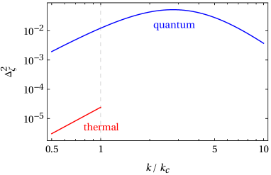
Figure 1: The quantum power spectrum (blue) and the thermal power spectrum (red) as a function of $k$ for $H/m=0.3$, $\alpha=1$, m$N_{F}=1$ and $\delta=0$.

As one can clearly see in this figure, thermal fluctuations significantly suppress the curvature perturbation spectrum with respect to the quantum case, for the reasons explained in the above section. Furthermore, whereas quantum vacuum fluctuations may yield a sufficiently large amplitude to lead to primordial black hole formation, a thermalized flaton field induces much smaller perturbations, although they may nevertheless exceed the even smaller fluctuations observed on large scales in the CMB anisotropies spectrum.

We should note that the quantum power spectrum peaks at scales that leave the horizon for $T<T_{c}$, where our approximations break down. Extending our calculation to this regime would involve a different form of the dissipation coefficient, since as the field experiences a tachyonic instability the latter no longer corresponds to the perturbative decay width at finite temperature. Let us note, however, that fluctuation-dissipation effects are more pronounced at the start of thermal inflation as discussed earlier, so that they no longer play a significant role near $T_{c}$. If the field thermalizes at the onset of thermal inflation, it will nevertheless maintain an equilibrium distribution with a decreasing temperature due to inflationary expansion. Let us then compare the magnitude of field fluctuations at $T_{c}$ in both the quantum vacuum and thermal cases. The thermal variance is obtained by expanding the field in terms of its modes

$$\braket{\phi(\bm{x})\phi(\bm{y})}=\int\frac{d^{3}k}{(2\pi)^{3}}\frac{d^{3}k^{\prime}}{(2\pi)^{3}}\;\braket{\phi_{k}\phi_{k^{\prime}}}\exp(i\bm{k}\cdot\bm{x})\exp(i\bm{k}\cdot\bm{y})~{},$$ (4.2)

and using the field modes correlator (3.15), we obtain for the field variance in the thermalized limit:

$$\braket{\phi^{2}}_{\text{therm}}=\frac{2}{(2\pi)^{2}}\frac{T}{a}\int_{0}^{k_{\text{cutoff}}}dk\;\frac{k^{2}}{k^{2}+\alpha^{2}T_{c}^{2}}=\frac{T^{2}}{2\pi}\bigg{[}1-\frac{\alpha}{\pi}\arctan\bigg{(}\frac{\pi}{\alpha}\bigg{)}\bigg{]}~{},$$ (4.3)

which we note is only mildly dependent on the effective coupling $\alpha$, while the quantum one is given by [16]:

$$\braket{\phi^{2}}_{\text{quan}}=\bigg{(}\frac{H}{2\pi}\bigg{)}^{2}\frac{\Gamma^{2}(\nu)2^{2\nu}}{6\pi}\bigg{(}\frac{aH}{m}\bigg{)}^{2\nu}F\bigg{(}\nu,\frac{3}{2};\frac{5}{2};-\bigg{(}\frac{aH}{m}\bigg{)}^{2}\bigg{)}~{},$$ (4.4)

where $F(a,b,c,z)$ denotes the Hypergeometric function. The field variance in both cases is shown in Figure 2, where we extrapolate the thermal variance beyond the phase transition purely for comparison purposes.

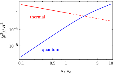
Figure 2: Quantum (blue) and thermal (red) field variance as a function of the scale factor for $H/m=0.3$, $\alpha=1$ and $\delta=0$. The critical temperature corresponds to the dashed vertical line, below which the thermal variance is extrapolated, as indicated by the dashed red line.

As one can clearly observe in this figure, the quantum field variance is several orders of magnitude smaller than the thermal variance before the phase transition, which validates our calculation in neglecting vacuum fluctuations in the thermalized flaton scenario. While at the critical temperature this is still true, if one extrapolates the thermal variance for $T<T_{c}$ ($a>a_{c}=1$), we see that quantum fluctuations become dominant less than one e-fold after the critical temperature is attained.

While this extrapolation is non-trivial, since the fluctuation-dissipation effects would have to be re-computed, it may suggest that vacuum perturbations may become dominant after the phase transition, in which case the computation in [16] would hold. In fact, the peak in the quantum power spectrum is obtained for modes with $k={H\over 2}\sqrt{3(2\nu+3)}>k_{c}=H$, which leave the horizon for temperatures below the critical value and thus, in the example shown above, already in the regime where the quantum variance is dominant.

This would, in fact, suggest that large enough curvature perturbations leading to primordial black hole formation may be generated after thermal inflation (from quantum fluctuations), but it is not clear that quantum and thermal fluctuations may be examined independently nor that the thermal variance maintains its form below $T_{c}$. In addition, and perhaps most importantly, the fact that the thermal variance is still typically a few orders of magnitude larger than the quantum one at the critical temperature indicates that the flaton field should reach the minimum of its potential much more quickly if it thermalizes, therefore considerably shortening, or even possibly, precluding an ensuing period of fast-roll inflation.

A more complete analysis of the problem including both thermal and quantum fluctuations in the analysis, potentially along the lines of [59], is required to compute the spectrum of curvature perturbations on scales that leave the horizon at temperatures below $T_{c}$, and is left for future work.

5 Conclusion

We have computed the spectrum of curvature perturbations generated during thermal inflation taking into account the thermal fluctuations of the flaton field driving this period. These are associated with fluctuation-dissipation effects driven by the flaton’s interactions with the ambient radiation bath. Our analysis involved solving the Langevin-like equation effectively describing the evolution of the flaton’s Fourier modes. We computed the associated correlation functions in the approximation of a gaussian white noise and a dominant thermal contribution to the flaton’s mass, for temperatures above the critical value at which the flaton is held at the false vacuum at the origin.

We have concluded that, if the flaton’s (finite-temperature) decay width exceeds the Hubble parameter at the onset of thermal inflation, the field essentially thermalizes with the ambient radiation bath, contributing approximately as an extra relativistic degree of freedom. This occurs when the effective coupling between the flaton and the thermalized degrees of freedom $\alpha\gtrsim 0.01$, which roughly corresponds to the parametric regime where over 10 e-folds of thermal inflation (above $T_{c}$) occur. We found that the consequent increase in the field variance and the average gradient and kinetic energies enhances the background energy density (namely its time-dependent part that determines curvature perturbations) with respect to a field with purely quantum vacuum fluctuations analyzed in [16]. Despite the enhancement of super-horizon density fluctuations in the thermal case, the overall amplitude of the curvature power spectrum is significantly reduced with respect to the quantum case, so that thermal fluctuations behave very differently compared to their quantum counterparts, regarding the generation of curvature perturbations during periods of thermal inflation.

While our analysis is not applicable for modes that leave the horizon once the temperature has fallen below the critical value and the field starts rolling towards the true minimum of its potential, we expect thermal effects to become less relevant in this regime and quantum fluctuations to become dominant, potentially yielding large curvature perturbations at such scales as computed in [16]. However, a full analysis including both quantum and thermal fluctuations in the dynamics of the flaton field is required to accurately describe the putative fast-roll inflation phase below the critical temperature. It must be noted, in any case, that such a phase is necessarily shortened by the fact that the field variance at the critical temperature, which sets the typical field value at this stage, is much larger if the field thermalizes with the radiation bath. It is therefore unclear whether super-horizon fluctuations with $k>k_{c}$ can be generated in this phase.

We have modelled the thermal bath through a set of fermion species coupled to the flaton field, but we expect our main conclusions to hold with the inclusion of other bosonic fields, like scalars or vector bosons: if $\Gamma_{\phi}>H$ at some stage during thermal inflation, the field will be driven towards a thermal fluctuation spectrum. Only the details of how and when this equilibrium is attained may depend on the types of light fields that interact with the flat direction. Our analysis shows that thermalization does not require large coupling constants describing the interaction between the flaton and the radiation bath. In any case such couplings cannot be too suppressed to sustain a sufficiently long period of thermal inflation that may, in particular, dilute any unwanted relics generated after the primary slow-roll inflation period. Hence, fluctuation-dissipation effects cannot in general be neglected in the dynamics of the flaton field and on the curvature perturbations they induce during thermal inflation. This is particularly relevant if one wishes to understand whether thermal inflation periods may leave behind a sizeable population of primordial black holes, and we hope that our work motivates further exploration of these and related issues, including other potential implications for structure formation in our Universe [60].

Appendix A Evolution of the temperature during thermal inflation

In our calculation we assumed that no significant entropy is produced during thermal inflation as a result of fluctuation-dissipation effects, i.e. that $T\propto a^{-1}$. In this appendix we aim to verify this assumption. The flaton field satisfies the Langevin-like equation [25]:

$$\ddot{\phi}+(3H+\Gamma_{\phi})\dot{\phi}-a^{-2}\nabla^{2}\phi+m_{\text{eff}}^{2}\phi=\xi~{},$$ (A.1)

and by multiplying both sides by $\dot{\phi}$ we obtain:

$$\dot{\rho}_{\phi}+3H(\rho_{\phi}+p_{\phi})=\xi\dot{\phi}-\Gamma_{\phi}\dot{\phi}^{2}+\alpha^{2}T\dot{T}\phi^{2}+a^{-2}\partial_{i}(\dot{\phi}\partial_{i}\phi)~{},$$ (A.2)

where the field’s energy density and pressure are given by:

$$\rho_{\phi} =\frac{1}{2}\dot{\phi}^{2}+\frac{1}{2}a^{-2}\partial_{i}\phi\partial_{i}\phi+V(\phi)~{},$$ (A.3)

$$p_{\phi} =\frac{1}{2}\dot{\phi}^{2}-\frac{1}{6}a^{-2}\partial_{i}\phi\partial_{i}\phi-V(\phi)~{}.$$

Conservation of the full energy-momentum tensor then yields the following continuity equation for the radiation energy density:

$$\dot{\rho}_{R}+4H\rho_{R}=-\braket{\xi\dot{\phi}}+\Gamma_{\phi}\braket{\dot{\phi}^{2}}-\alpha^{2}T\dot{T}\braket{\phi^{2}}-a^{-2}\braket{\partial_{i}(\dot{\phi}\partial_{i}\phi})~{}.$$ (A.4)

We note that the radiation energy density is an ensemble average over the energy density of the relativistic degrees of freedom, which justifies considering also the thermal average of the terms on the right-hand side of the above equation. Here we have also neglected the sub-leading corrections to the radiation energy and entropy densities from the fermions’ finite mass, $\sim g\braket{\sqrt{\phi^{2}}}\sim gT\ll T$.

Using the field solutions we obtained for the correlators:

$$\braket{\xi\dot{\phi}} =\frac{\pi}{6}\Gamma_{\phi}T^{4}~{},$$ (A.5)

$$\Gamma_{\phi}\braket{\dot{\phi}^{2}} =\frac{\pi}{6}\Gamma_{\phi}T^{4}(1-\delta)~{},$$

$$\alpha^{2}T\dot{T}\braket{\phi^{2}} =\frac{\alpha^{2}}{2\pi}T^{3}\dot{T}\bigg{[}1-\frac{\alpha}{\pi}\arctan\bigg{(}\frac{\pi}{\alpha}\bigg{)}\bigg{]}(1-\delta)\approx\frac{15\alpha^{2}}{4\pi^{3}g_{*}}(1-\delta)\dot{\rho}_{R}~{},$$

$$\braket{\partial_{i}(\dot{\phi}\partial_{i}\phi} =0~{}.$$

Note that the third term is related to the time-dependence of the thermal flaton mass, and yields a contribution to the variation of the radiation energy density comparable to the above-mentioned sub-leading corrections from the fermions’ non-vanishing mass. For consistency, we thus neglect this term, and obtain:

$$\dot{\rho}_{R}+4H\rho_{R}=-{5/\pi\over g_{*}}\Gamma_{\phi}\rho_{R}\delta~{}.$$ (A.6)

From this we immediately see that the right-hand side can only be significant if $\Gamma_{\phi}\gtrsim H$, but this implies a quick thermalization of the flaton field such that $\delta\to 0$ exponentially fast, thus making this term negligible. This simply reflects the balance between the effects of fluctuations and dissipation as the flaton field reaches an equilibrium with the radiation bath. Note, furthermore, that the term on the right-hand side is suppressed by the relative contribution of the flaton to the number of relativistic species in equilibrium, $(g_{*,f}-g_{*})/g_{*}$, as obtained in Section 3. We therefore conclude that one may consistently assume $\rho_{R}\propto a^{-4}$ and hence that $T\propto a^{-1}$ during thermal inflation.

Appendix B Field correlation functions

Here we list the field correlation functions used to compute the curvature perturbation power spectrum. As we mentioned above, when integrating over momentum modes we consider a sharp cut-off at $k=\pi T_{c}$, which constitutes a good approximation to the behaviour of the noise correlation function [46]. To compute the curvature perturbation power spectrum on super-horizon scales, $k\ll aH$, we consider the leading order results in $k/\alpha T_{c}\sim(k/aH)(M_{0}/M_{P})a\ll 1$ considering $M_{0}<M_{P}$ and noting that in our convention $a<a_{c}=1$ above the critical temperature.

Mode correlators

The building blocks of all field correlators are the equal time correlators between the field modes and their time derivatives. Writing $\phi_{k}$ and $\dot{\phi}_{k}$ in terms of the Green’s function (3.13):

$$\phi_{k} =H^{-2}\int_{z_{i}}^{z}ds\;s^{-2}G_{s}(z,s)\xi_{k}(s)~{},$$ (B.1)

$$\dot{\phi}_{k} =H^{-1}z\int_{z_{i}}^{z}ds\;s^{-2}\partial_{z}G_{s}(z,s)\xi_{k}(s)~{},$$

one finds:

$$\braket{\phi_{k}\phi_{k^{\prime}}} =(2\pi)^{3}\delta^{3}(\bm{k}+\bm{k}^{\prime})\frac{T}{a^{3}\omega_{k}^{2}}(1-\delta)~{},$$ (B.2)

$$\braket{\dot{\phi}_{k}\dot{\phi}_{k^{\prime}}} =(2\pi)^{3}\delta^{3}(\bm{k}+\bm{k}^{\prime})\frac{T}{a^{3}}(1-\delta)~{},$$

$$\braket{\phi_{k}\dot{\phi}_{k^{\prime}}} =-\frac{\Gamma_{\phi}}{2}\braket{\phi_{k}\phi_{k^{\prime}}}=-(2\pi)^{3}\delta^{3}(\bm{k}+\bm{k}^{\prime})\frac{T\Gamma_{\phi}}{2a^{3}\omega_{k}^{2}}(1-\delta)~{}.$$

Field correlators

To compute the total energy density (3.4a) one needs to determine the field variance and the average kinetic and gradient energies. Expanding the field in terms of comoving momentum modes, these are given by:

$$\braket{\phi^{2}} =\int\frac{d^{3}k}{(2\pi)^{3}}\frac{d^{3}k^{\prime}}{(2\pi)^{3}}\braket{\phi_{k}\phi_{k^{\prime}}}\exp(i\bm{x}\cdot(\bm{k}+\bm{k}^{\prime}))~{},$$ (B.3)

$$\braket{\dot{\phi}^{2}} =\int\frac{d^{3}k}{(2\pi)^{3}}\frac{d^{3}k^{\prime}}{(2\pi)^{3}}\braket{\dot{\phi}_{k}\dot{\phi}_{k^{\prime}}}\exp(i\bm{x}\cdot(\bm{k}+\bm{k}^{\prime}))~{},$$

$$\braket{\partial_{i}\phi\partial_{i}\phi} =\int\frac{d^{3}k}{(2\pi)^{3}}\frac{d^{3}k^{\prime}}{(2\pi)^{3}}\braket{\phi_{k}\phi_{k^{\prime}}}\bm{k}\cdot\bm{k}^{\prime}\exp(i\bm{x}\cdot(\bm{k}+\bm{k}^{\prime}))~{}.$$

Inserting the mode correlation functions (B.2) and integrating over comoving momenta up to $\pi T_{c}$ one obtains:

$$\braket{\phi^{2}} =\frac{T^{2}}{2\pi}(1-\delta)\bigg{[}1-\frac{\alpha}{\pi}\arctan\bigg{(}\frac{\pi}{\alpha}\bigg{)}\bigg{]}~{},$$ (B.4)

$$\braket{\dot{\phi}^{2}} =\frac{\pi T^{4}}{6}(1-\delta)~{},$$

$$\braket{\partial_{i}\phi\partial_{i}\phi} =\frac{\pi}{2}a^{2}T^{4}(1-\delta)\bigg{[}\frac{1}{3}-\bigg{(}\frac{\alpha}{\pi}\bigg{)}^{2}+\bigg{(}\frac{\alpha}{\pi}\bigg{)}^{3}\arctan\bigg{(}\frac{\pi}{\alpha}\bigg{)}\bigg{]}~{}.$$

Contributions to the power spectrum

Consider the power spectrum of a generic correlator $\braket{X_{i}(0)X_{j}(\bm{x})}$, for example $X_{1}=\phi$, $X_{2}=\dot{\phi}$ and $X_{3}=\partial_{i}\phi$, that appears in (3.7):

$$\int d^{3}x\exp(-i\bm{k}\cdot\bm{x})\braket{X_{i}(0)X_{j}(\bm{x})}^{2}~{}.$$ (B.5)

Note that, upon expanding each quantity $X_{j}(\mathbf{x})$ in terms of comoving momentum modes, this yields four momentum integrals and a volume integral. Two of the momentum integrals can be performed using the two delta functions appearing in the mode correlators (B.2). Then, the volume integral will generate a delta function with the two surviving momentum modes:

$$\int d^{3}x\;\exp[-i\bm{x}\cdot(\bm{k}_{1}+\bm{k}_{2}+\bm{k})]=(2\pi)^{3}\delta^{3}(\bm{k}_{1}+\bm{k}_{2}+\bm{k})~{}.$$ (B.6)

After integrating this delta function over another of the 3-momentum variables, we are left with a single 3-dimensional integral over $\bm{k}$ that we need to compute in each case. In the following table we give the different contributions to the power spectrum in terms of their corresponding momentum integrals:

Table 1: Contributions to the power spectrum in Eq. (3.17).

field-field	$\frac{m_{\text{eff}}^{4}}{2}\int d^{3}x\;\exp(-i\bm{k}\cdot\bm{x})\braket{\phi(0)\phi(\bm{x})}^{2}$	$(1-\delta)^{2}\frac{\alpha^{3}}{2(2\pi)^{3}}\frac{T^{5}}{a^{3}}I_{1}(k)$
field-kinetic	$m_{\text{eff}}^{2}\int d^{3}x\;\exp(-i\bm{k}\cdot\bm{x})\braket{\phi(0)\dot{\phi}(\bm{x})}^{2}$	$(1-\delta)^{2}\frac{\alpha}{(2\pi)^{3}}\big{(}\frac{3\alpha^{4}}{32\pi}\big{)}^{2}\frac{T^{5}}{a^{3}}I_{1}(k)$
field-gradient	$a^{-2}m_{\text{eff}}^{2}\int d^{3}x\;\exp(-i\bm{k}\cdot\bm{x})\braket{\phi(0)\partial_{i}\phi(\bm{x})}^{2}$	$(1-\delta)^{2}\frac{\alpha^{3}}{(2\pi)^{3}}\frac{T^{5}}{a^{3}}I_{2}(k)$
kinetic-kinetic	$\frac{1}{2}\int d^{3}x\;\exp(-i\bm{k}\cdot\bm{x})\braket{\dot{\phi}(0)\dot{\phi}(\bm{x})}^{2}$	$(1-\delta)^{2}\frac{\alpha^{3}}{2(2\pi)^{3}}\frac{T^{5}}{a^{3}}I_{3}(k)$
kinetic-gradient	$a^{-2}\int d^{3}x\;\exp(-i\bm{k}\cdot\bm{x})\braket{\dot{\phi}(0)\partial_{i}\phi(\bm{x})}^{2}$	$(1-\delta)^{2}\frac{\alpha}{(2\pi)^{3}}\big{(}\frac{3\alpha^{4}}{32\pi}\big{)}^{2}\frac{T^{5}}{a^{3}}I_{2}(k)$
gradient-gradient	$\frac{a^{-4}}{2}\int d^{3}x\;\exp(-i\bm{k}\cdot\bm{x})\braket{\partial_{i}\phi(0)\partial_{j}\phi(\bm{x})}^{2}$	$(1-\delta)^{2}\frac{\alpha^{3}}{2(2\pi)^{3}}\frac{T^{5}}{a^{3}}I_{4}(k)$

The momentum integrals can be expressed in terms of the normalized comoving momentum $\bm{y}=\bm{k}/\alpha T_{c}$ with norm $0<y<\pi/\alpha$. These are given by:

$$I_{1}(k) =\int dy\,d\Omega\;\frac{y^{2}}{(y^{2}+1)[(\bm{y}+\bm{k}/(\alpha T_{c}))^{2}+1]}~{},$$ (B.7)

$$I_{2}(k) =\int dy\,d\Omega\;\frac{y^{2}\bm{y}\cdot(\bm{y}+\bm{k}/(\alpha T_{c}))}{(y^{2}+1)[(\bm{y}+\bm{k}/(\alpha T_{c}))^{2}+1]}~{},$$

$$I_{3}(k) =\int dy\,d\Omega\;y^{2}=\frac{4\pi^{4}}{3\alpha^{3}}~{},$$

$$I_{4}(k) =\int dy\,d\Omega\;\frac{y^{2}[\bm{y}\cdot(\bm{y}+\bm{k}/(\alpha T_{c}))]^{2}}{(y^{2}+1)[(\bm{y}+\bm{k}/(\alpha T_{c}))^{2}+1]}~{},$$

where $d\Omega$ denotes integration over the solid angle in momentum space. Except for $I_{3}(k)$, all integrals above depend non-trivially on $k$. To leading order in $k/\alpha T_{c}$ these integrals are given by:

$$I_{1}(k) \simeq 4\pi\bigg{[}-\frac{1}{2}\frac{\pi\alpha}{\alpha^{2}+\pi^{2}}+\frac{1}{2}\arctan(\pi/\alpha)\bigg{]}~{},$$ (B.8)

$$I_{2}(k) \simeq 4\pi\bigg{[}\frac{\pi}{\alpha}+\frac{1}{2}\frac{\alpha\pi}{\alpha^{2}+\pi^{2}}-\frac{3}{2}\arctan(\pi/\alpha)\bigg{]}~{},$$

$$I_{4}(k) \simeq 4\pi\bigg{[}-\frac{2\pi}{\alpha}+\frac{1}{3}\frac{\pi^{3}}{\alpha^{3}}-\frac{1}{2}\frac{\alpha\pi}{\alpha^{2}+\pi^{2}}+\frac{5}{2}\arctan(\pi/\alpha)\bigg{]}~{},$$

which are the expressions used to compute the curvature perturbation power spectrum (3.17) given in the main body of this article.

References

- [1] A.A. Starobinsky, A New Type of Isotropic Cosmological Models Without Singularity, Phys. Lett. B 91 (1980) 99.
- [2] K. Sato, First Order Phase Transition of a Vacuum and Expansion of the Universe, Mon. Not. Roy. Astron. Soc. 195 (1981) 467.
- [3] A.H. Guth, The Inflationary Universe: A Possible Solution to the Horizon and Flatness Problems, Phys. Rev. D 23 (1981) 347.
- [4] A.D. Linde, A New Inflationary Universe Scenario: A Possible Solution of the Horizon, Flatness, Homogeneity, Isotropy and Primordial Monopole Problems, Phys. Lett. B 108 (1982) 389.
- [5] J. Rocher and M. Sakellariadou, Supersymmetric grand unified theories and cosmology, JCAP 03 (2005) 004 [hep-ph/0406120].
- [6] H. Pagels and J.R. Primack, Supersymmetry, Cosmology and New TeV Physics, Phys. Rev. Lett. 48 (1982) 223.
- [7] S. Weinberg, Cosmological Constraints on the Scale of Supersymmetry Breaking, Phys. Rev. Lett. 48 (1982) 1303.
- [8] M.Y. Khlopov and A.D. Linde, Is It Easy to Save the Gravitino?, Phys. Lett. B 138 (1984) 265.
- [9] M. Kawasaki, K. Kohri, T. Moroi and A. Yotsuyanagi, Big-Bang Nucleosynthesis and Gravitino, Phys. Rev. D 78 (2008) 065011 [0804.3745].
- [10] L. Randall and S.D. Thomas, Solving the cosmological moduli problem with weak scale inflation, Nucl. Phys. B 449 (1995) 229 [hep-ph/9407248].
- [11] D.H. Lyth and E.D. Stewart, Cosmology with a TeV mass GUT Higgs, Phys. Rev. Lett. 75 (1995) 201 [hep-ph/9502417].
- [12] D.H. Lyth and E.D. Stewart, Thermal inflation and the moduli problem, Phys. Rev. D 53 (1996) 1784 [hep-ph/9510204].
- [13] T. Asaka and M. Kawasaki, Cosmological moduli problem and thermal inflation models, Phys. Rev. D 60 (1999) 123509 [hep-ph/9905467].
- [14] T. Barreiro, E.J. Copeland, D.H. Lyth and T. Prokopec, Some aspects of thermal inflation: The Finite temperature potential and topological defects, Phys. Rev. D 54 (1996) 1379 [hep-ph/9602263].
- [15] T. Gherghetta, C.F. Kolda and S.P. Martin, Flat directions in the scalar potential of the supersymmetric standard model, Nucl. Phys. B 468 (1996) 37 [hep-ph/9510370].
- [16] K. Dimopoulos, T. Markkanen, A. Racioppi and V. Vaskonen, Primordial Black Holes from Thermal Inflation, JCAP 07 (2019) 046 [1903.09598].
- [17] A.D. Linde, Fast roll inflation, JHEP 11 (2001) 052 [hep-th/0110195].
- [18] B. Carr and F. Kuhnel, Primordial black holes as dark matter candidates, SciPost Phys. Lect. Notes 48 (2022) 1 [2110.02821].
- [19] A. Berera, Warm inflation, Phys. Rev. Lett. 75 (1995) 3218 [astro-ph/9509049].
- [20] A. Berera and L.-Z. Fang, Thermally induced density perturbations in the inflation era, Phys. Rev. Lett. 74 (1995) 1912 [astro-ph/9501024].
- [21] A. Berera, M. Gleiser and R.O. Ramos, Strong dissipative behavior in quantum field theory, Phys. Rev. D 58 (1998) 123508 [hep-ph/9803394].
- [22] A. Berera, M. Gleiser and R.O. Ramos, A First principles warm inflation model that solves the cosmological horizon / flatness problems, Phys. Rev. Lett. 83 (1999) 264 [hep-ph/9809583].
- [23] A. Berera, Warm inflation at arbitrary adiabaticity: A Model, an existence proof for inflationary dynamics in quantum field theory, Nucl. Phys. B 585 (2000) 666 [hep-ph/9904409].
- [24] A. Berera and R.O. Ramos, The Affinity for scalar fields to dissipate, Phys. Rev. D 63 (2001) 103509 [hep-ph/0101049].
- [25] A. Berera, I.G. Moss and R.O. Ramos, Warm Inflation and its Microphysical Basis, Rept. Prog. Phys. 72 (2009) 026901 [0808.1855].
- [26] M. Bastero-Gil and A. Berera, Warm inflation model building, Int. J. Mod. Phys. A 24 (2009) 2207 [0902.0521].
- [27] M. Bastero-Gil, A. Berera and R.O. Ramos, Dissipation coefficients from scalar and fermion quantum field interactions, JCAP 09 (2011) 033 [1008.1929].
- [28] M. Bastero-Gil, A. Berera and J.G. Rosa, Warming up brane-antibrane inflation, Phys. Rev. D 84 (2011) 103503 [1103.5623].
- [29] M. Bastero-Gil, A. Berera, R.O. Ramos and J.G. Rosa, Warm baryogenesis, Phys. Lett. B 712 (2012) 425 [1110.3971].
- [30] M. Bastero-Gil, A. Berera, R.O. Ramos and J.G. Rosa, General dissipation coefficient in low-temperature warm inflation, JCAP 01 (2013) 016 [1207.0445].
- [31] S. Bartrum, M. Bastero-Gil, A. Berera, R. Cerezo, R.O. Ramos and J.G. Rosa, The importance of being warm (during inflation), Phys. Lett. B 732 (2014) 116 [1307.5868].
- [32] M. Bastero-Gil, A. Berera, I.G. Moss and R.O. Ramos, Cosmological fluctuations of a random field and radiation fluid, JCAP 05 (2014) 004 [1401.1149].
- [33] M. Bastero-Gil, A. Berera, R.O. Ramos and J.G. Rosa, Warm Little Inflaton, Phys. Rev. Lett. 117 (2016) 151301 [1604.08838].
- [34] J.a.G. Rosa and L.B. Ventura, Warm Little Inflaton becomes Cold Dark Matter, Phys. Rev. Lett. 122 (2019) 161301 [1811.05493].
- [35] M. Bastero-Gil, A. Berera, R.O. Ramos and J.a.G. Rosa, Towards a reliable effective field theory of inflation, Phys. Lett. B 813 (2021) 136055 [1907.13410].
- [36] K.V. Berghaus, P.W. Graham and D.E. Kaplan, Minimal Warm Inflation, JCAP 03 (2020) 034 [1910.07525].
- [37] M. Bastero-Gil, A. Berera, R. Brandenberger, I.G. Moss, R.O. Ramos and J.G. Rosa, The role of fluctuation-dissipation dynamics in setting initial conditions for inflation, JCAP 01 (2018) 002 [1612.04726].
- [38] S. Bartrum, A. Berera and J.G. Rosa, Fluctuation-dissipation dynamics of cosmological scalar fields, Phys. Rev. D 91 (2015) 083540 [1412.5489].
- [39] J.a.G. Rosa and L.B. Ventura, Spontaneous breaking of the Peccei-Quinn symmetry during warm inflation, 2105.05771.
- [40] M. Dine, L. Randall and S.D. Thomas, Baryogenesis from flat directions of the supersymmetric standard model, Nucl. Phys. B 458 (1996) 291 [hep-ph/9507453].
- [41] G.R. Dvali and Q. Shafi, Gauge hierarchy, Planck scale corrections and the origin of GUT scale in supersymmetric SU(3)**3, Phys. Lett. B 339 (1994) 241 [hep-ph/9404334].
- [42] L. Dolan and R. Jackiw, Symmetry Behavior at Finite Temperature, Phys. Rev. D 9 (1974) 3320.
- [43] K. Yamamoto, Phase Transition Associated With Intermediate Gauge Symmetry Breaking in Superstring Models, Phys. Lett. B 168 (1986) 341.
- [44] L. Kofman, A.D. Linde and A.A. Starobinsky, Reheating after inflation, Phys. Rev. Lett. 73 (1994) 3195 [hep-th/9405187].
- [45] K. Dimopoulos and C. Owen, How Thermal Inflation can save Minimal Hybrid Inflation in Supergravity, JCAP 10 (2016) 020 [1606.06677].
- [46] T. Hiramatsu, Y. Miyamoto and J. Yokoyama, Effects of thermal fluctuations on thermal inflation, JCAP 03 (2015) 024 [1412.7814].
- [47] E.A. Calzetta and B.-L.B. Hu, Nonequilibrium Quantum Field Theory, Cambridge Monographs on Mathematical Physics, Cambridge University Press (9, 2008), 10.1017/CBO9780511535123.
- [48] I.G. Moss and C.M. Graham, Particle production and reheating in the inflationary universe, Phys. Rev. D 78 (2008) 123526 [0810.2039].
- [49] M. Gleiser and R.O. Ramos, Microphysical approach to nonequilibrium dynamics of quantum fields, Phys. Rev. D 50 (1994) 2441 [hep-ph/9311278].
- [50] J.M. Bardeen, P.J. Steinhardt and M.S. Turner, Spontaneous Creation of Almost Scale - Free Density Perturbations in an Inflationary Universe, Phys. Rev. D 28 (1983) 679.
- [51] D. Baumann, Inflation, in Theoretical Advanced Study Institute in Elementary Particle Physics: Physics of the Large and the Small, pp. 523–686, 2011, DOI [0907.5424].
- [52] E.W. Kolb and M.S. Turner, The Early Universe, vol. 69, CRC Press (1990), 10.1201/9780429492860.
- [53] L. Isserlis, On a formula for the product-moment coefficient of any order of a normal frequency distribution in any number of variables, 11, 1918. 10.2307/2331932.
- [54] C. Vignat, A generalized isserlis theorem for location mixtures of gaussian random vectors, Statistics & Probability Letters 82 (2012) 67–71 [1107.2309].
- [55] M. Abramowitz and I.A. Stegun, Handbook of Mathematical Functions, National Bureau of Standards, 10th edition ed. (1972).
- [56] A.M. Green and A.R. Liddle, Constraints on the density perturbation spectrum from primordial black holes, Phys. Rev. D 56 (1997) 6166 [astro-ph/9704251].
- [57] M.Y. Khlopov, Primordial Black Holes, Res. Astron. Astrophys. 10 (2010) 495 [0801.0116].
- [58] A.M. Green, Primordial Black Holes: sirens of the early Universe, Fundam. Theor. Phys. 178 (2015) 129 [1403.1198].
- [59] R.O. Ramos and L.A. da Silva, Power spectrum for inflation models with quantum and thermal noises, JCAP 03 (2013) 032 [1302.3544].
- [60] M. Leo, C.M. Baugh, B. Li and S. Pascoli, N-body simulations of structure formation in thermal inflation cosmologies, JCAP 12 (2018) 010 [1807.04980].