Causal structure and the geodesics in the hairy extension of the Bertotti-Robinson spacetime

Abstract

A hairy extension of the Bertotti-Robinson regular spacetime has been recently introduced in the context of the Einstein-Maxwell-Scaler theory that surprisingly is a singular black hole formed in the $S_{3}$ background spatial topology [CQG39(2022)167001]. In this research, we first clarify the topology of the spacetime based on the coordinate transformations as well as the energy-momentum configuration and the causal structure of the black hole. Furthermore, we investigate the geodesics of the null and timelike particles in this spacetime. It is shown that in the radial motion on the equatorial plane, while photons may collapse to the singularity or escape to the edge of the universe, a massive particle always collapses to the singularity. The general geodesics of null and massive particles reveal that all particles except the outgoing light ray, eventually fall into the black hole.

I Introduction

In general relativity, no-hair theorems state that black holes are described by only three parameters, their mass $M$, their electromagnetic charge $Q$, and their angular momentum $\ell$ 1 ; 2 ; 3 ; 4 ; 5 . Recent studies on black holes indicate the existence of hairy black holes some of which form in the presence of Yang-Mills fields 7 ; 8 ; 9 . Hairy black holes are solutions to Einstein’s equations in the interaction of diverse kinds of matter fields with gravity 10 . For instance gravity in interaction with electromagnetism and axion 11 ; 12 ; 13 , gravity coupled to electromagnetism and dilaton 14 ; 15 ; 16 ; 17 , and gravity in interaction with electromagnetism and Abelian Higgs field 18 . The first study on the coupling of gravity and a scalar field was considered by Fisher who presented a static and spherically symmetric solution in the theory Fisher . It is known that the string theory in the low energy limit reduces to Einstein’s theory coupled nontrivially to other fields such as axion, dilaton, and gauge fields Dil . Such coupling for instance in Einstein-Maxwell-Dilaton (EMD) theory changes significantly the physical characteristics of the black hole such as the causal structure, the asymptotic behavior and the thermodynamics from the Reissner-Nordström black hole Dil2 ; Dil3 . Several exact black hole solutions in EMD theory have been obtained that are either asymptotically flat AF1 ; AF2 ; AF3 ; AF4 ; AF5 ; AF6 ; AF7 or non-asymptotically flat NF1 ; NF2 ; NF3 ; NF4 ; NF5 ; NF6 ; NF7 ; NF8 ; NF9 ; NF10 ; NF11 ; NF12 ; NF13 ; NF14 ; NF15 . Among the non-asymptotically flat solutions, some are asymptotically de-Sitter or anti-de Sitter ds1 ; ds2 ; ds3 ; ds4 ; ds5 ; ds6 ; ds7 ; ds8 ; ds9 ; ds10 ; ds11 which have applications in the anti-de Sitter, conformal field theory correspondence (AdS/CFT) in the context of the unification of the quantum field theory and gravitation CFT . We note that EMD is not the only extension of the Einstein-Maxwell (EM) theory and the coupling of gravity to scalar fields through Maxwell’s gauge i.e., Einstein-Maxwell-Scalar (EMS) theory, has also received great attention in the literature EMS ; S2 ; S3 ; S4 ; S5 ; S6 ; S7 ; S8 ; S9 ; S10 . For a good classification of EMS theory, we refer to a recent paper by Astefanesei et al S11 . Besides the theory of scalar/dilaton coupled to gravity, the scalar-tensor theory of gravity with the Higgs field as the scalar field has been studied in different contexts such as the flat rotation curves anomaly of spiral galaxies H1 , and the Higgs field as quintessence H2 . In H3 horizon-less spherically symmetric vacuum solutions have been introduced in the Higgs scalar-tensor theory of gravity such that in the vanishing limit of the Higgs field excitations, the usual Schwarzschild black hole is recovered.

In this current study, we investigate further the hairy extension of the Bertotti-Robinson (BR) spacetime 19 ; 20 ; 21 ; 22 ; 23 ; 24 ; R1 ; R2 in the context of the EM theory 25 , a subgroup of hairy black holes which have gravity in interaction with electromagnetism and scalar fields 26 . This new spacetime eventuates a black hole in closed space. One of the reasons to study a closed space in a cosmological sense is that the energy and the topology of an open universe are difficult to be determined. Moreover, a static, closed space can depict information related to the dynamics of the universe and an early universe 27 . One of the well-known cosmological models of the universe is the Robertson-Walker (RW) WR metric which is described by

$$ds_{RW}^{2}=-dt^{2}+a\left(t\right)^{2}\left(dr^{2}+S_{K}\left(r\right)^{2}\left(d\theta^{2}+\sin^{2}\theta d\varphi^{2}\right)\right)$$ (1)

where

$$S_{K}\left(r\right)=\left\{\begin{array}[]{ccc}r&&K=0\\ \sin r&&K=+1\\ \sinh r&&K=-1\end{array}\right.$$ (2)

and $K$ stands for the spatial Gaussian curvature. Considering the topology of the universe (1) to be $\mathbb{R}\times\Sigma$ with $\mathbb{R}$ representing the time and $\Sigma$ the spatial three-manifold, $K=0,-1$ and $+1$ imply that $\Sigma$ is flat, open or closed, respectively. Applying the transformation given by $S_{K}\left(r\right)^{2}\rightarrow R^{2}$ the line element (1) becomes

$$ds_{RW}^{2}=-dt^{2}+a\left(t\right)^{2}\left(\frac{dR^{2}}{1-KR^{2}}+R^{2}\left(d\theta^{2}+\sin^{2}\theta d\varphi^{2}\right)\right).$$ (3)

With $K=+1,$ (3) represents a closed universe in the sense that $R$ is confined to $R\in\left[0,\sqrt{\frac{1}{K}}\right).$ Furthermore, assuming $a\left(t\right)=a_{0}=const.,$ (3) becomes a static closed universe upon which Einstein’s field equation $G_{\mu}^{\nu}=T_{\mu}^{\nu}$ yields

$$T_{\mu}^{\nu}=diag\left[-\rho_{0},p_{0},p_{0},p_{0}\right]$$ (4)

where the energy density and the pressure are given by $\rho_{0}=\frac{3K}{a_{0}^{2}}$ and $p_{0}=-\frac{K}{a_{0}^{2}},$ respectively. The equation of state (EoS) of the perfect fluid supporting the above static universe is given by

$$p_{0}=-\frac{\rho_{0}}{3}.$$ (5)

It is clear that with $K=0$ the flat universe is a vacuum, with $K=+1$ the closed universe is supported by a physical isotropic matter field whose positive energy density (with finite total energy) and negative isotropic pressure (with vanishing gravitational mass density, $\rho_{G}=\rho_{0}+3p_{0}$) satisfy all the energy conditions including the null energy condition ($\rho_{0}+p_{0}\geq 0$), the weak energy condition ($\rho_{0}\geq 0,\rho_{0}+p_{0}\geq 0$) and the strong energy condition ($\rho_{0}+3p_{0}\geq 0$). On the other hand, with $K=-1$ the open universe is supported by an exotic matter with a negative energy density (with an infinite total exotic matter) and a positive isotropic pressure (which pushes the universe away from the center), and all energy conditions are violated.

Studying the geodesics of the massless or massive particles in the vicinity of the black holes plays a great role in understanding the structure of their spacetime geometry. Such investigations around different black holes have been published in literature ever since the first black hole was introduced. Here G1 ; G2 ; G3 ; G4 ; G5 ; G6 ; G7 ; G8 ; G9 ; G10 ; G11 ; G12 ; G13 ; G14 ; G15 , we refer to some of them and the interested reader can find more in their references as well. In this context, we are going to study geodesics equations of a test particle in the spacetime of the black hole powered by pure magnetic fields introduced in 25 . The main streamline of the present work is to investigate the trajectory of massless/null and massive/timelike test particles. We derive the energy and angular momentum of the test particles and we illustrate some observable quantities in graphs to discover the particle’s behavior in different circumstances.

The organization of the paper is as follows. In Sec. II we present a review of the action, the field equations, and the black hole solution obtained previously in 25 . Sec. III is devoted to the topology of the mentioned spacetime and in particular, we concentrate on the formation of the black hole in $S_{3}$ background spatial topology, from different aspects including the energy conditions, the causal structure, and the Penrose diagram. In Sec. IV the geodesics equation of the null and massive particles are analyzed and the results are presented either analytically or numerically through some graphs. Finally in Sec. V the paper is concluded by remarking on the results.

II A review on the hairy extension of the BR spacetime

The black hole solution reported in 25 has been obtained in the context of EMS theory where the action is given by ($8\pi G=c=1$)

$$I=\frac{1}{2}\int d^{4}x\sqrt{-g}\left(\mathcal{R}-2\partial_{\mu}\psi\partial^{\mu}\psi+V_{0}\cos\left(\frac{\psi}{\sqrt{2}}\right)F_{\mu\nu}F^{\mu\nu}\right)$$ (6)

in which $\psi$ is the scalar field, $V_{0}$ is a positive coupling constant, $\mathcal{R}$ is the Ricci scalar and $F_{\mu\nu}F^{\mu\nu}$ is Maxwell’s invariant. Variation of the action with respect to $g_{\mu\nu},$ $A_{\mu}$ and $\psi,$ respectively, yields the field equations given by

$$\mathcal{R}_{\mu}^{\nu}=2\partial_{\mu}\psi\partial^{\nu}\psi+\frac{1}{2}V_{0}\cos\left(\frac{\psi}{\sqrt{2}}\right)\left(4F_{\mu\lambda}F^{\nu\lambda}-F_{\alpha\beta}F^{\alpha\beta}\delta_{\mu}^{\nu}\right),$$ (7)

$$\nabla_{\mu}\left(V_{0}\cos\left(\frac{\psi}{\sqrt{2}}\right)F^{\mu\nu}\right)=0$$ (8)

and

$$\nabla_{\mu}\nabla^{\mu}\psi=-\frac{V_{0}}{4\sqrt{2}}\sin\left(\frac{\psi}{\sqrt{2}}\right)F_{\mu\nu}F^{\mu\nu}.$$ (9)

The electromagnetic gauge field is considered to be a pure radial magnetic field produced by a magnetic monopole sitting at the origin such that

$$\mathbf{F}=P\sin\theta d\theta\wedge d\varphi$$ (10)

where the constant parameter $P$ is the magnetic charge. For the method upon which the field equations have been solved, we refer to the original paper in Ref. 25 where all the details can be found. Hence, we only write the solutions which are as follow. The spacetime is spherically symmetric with the line element

$$ds^{2}=-f\left(r\right)dt^{2}+\frac{dr^{2}}{f\left(r\right)}+R\left(r\right){}^{2}d\Omega^{2},$$ (11)

in which the metric functions are given by

$$f\left(r\right)=\frac{\left(r+r_{h}\right){}^{3}\left(r-r_{h}\right)}{R_{0}^{2}r^{2}},$$ (12)

and

$$R\left(r\right)=R_{0}\left(\frac{r}{r+r_{h}}\right).$$ (13)

Furthermore, the radial magnetic field and the scalar field are obtained to be

$$B\left(r\right)=\frac{P\left(r+r_{h}\right)^{2}}{R_{0}^{2}r^{2}},$$ (14)

and

$$\psi\left(r\right)=\pm 2\sqrt{2}\arctan\left(\sqrt{\frac{r}{r_{h}}}\right),$$ (15)

respectively. Herein, $r_{h}$ is the event horizon and $R_{0}^{2}=P^{2}V_{0}$. The scalar field (15) becomes constant as $r_{h}\rightarrow 0$ i.e.,

$$\psi\left(r\right)\rightarrow\pm\sqrt{2}\pi\text{ \ as }r_{h}\rightarrow 0$$ (16)

and consequently

$$V_{0}\cos\left(\frac{\psi}{\sqrt{2}}\right)F_{\mu\nu}F^{\mu\nu}\rightarrow-V_{0}F_{\mu\nu}F^{\mu\nu}$$ (17)

which upon setting $V_{0}=1$ the action reduces to EM theory, and the spacetime becomes

$$ds^{2}=-\frac{r^{2}}{P^{2}}dt^{2}+\frac{P^{2}dr^{2}}{r^{2}}+P^{2}d\Omega^{2}.$$ (18)

This line element is not the Reissner-Nordström black hole solution of the EM theory. Instead, the transformations $r=\frac{1}{\tilde{r}}$ and $t=P\tilde{t}$ yield

$$ds^{2}=\frac{P^{2}}{\tilde{r}^{2}}\left(-d\tilde{t}^{2}+d\tilde{r}^{2}+\tilde{r}^{2}d\Omega^{2}\right)$$ (19)

which reveals that (18) is the regular solution of the EM theory known as the BR spacetime 19 ; 20 .

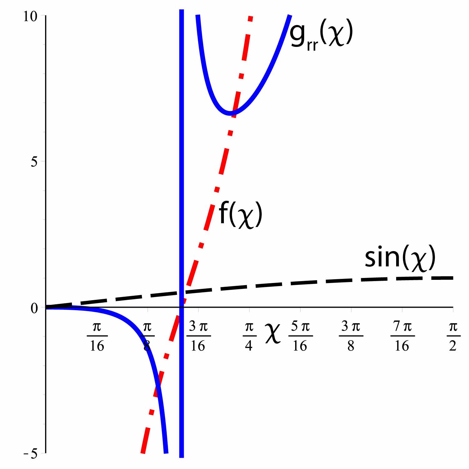
Figure 1: The plots of scaled transformed metric function i.e., $\frac{R_{0}^{2}}{r_{h}^{2}}f\left(\chi\right)$ (red, dash-dot), as well as $\frac{1}{R_{0}^{2}}g_{\chi\chi}$ from (27) (blue, solid) and $\sin\chi$ (dash) for $0\leq\chi\leq\frac{\pi}{2}$.

III Black hole in the $S_{3}$ space topology background

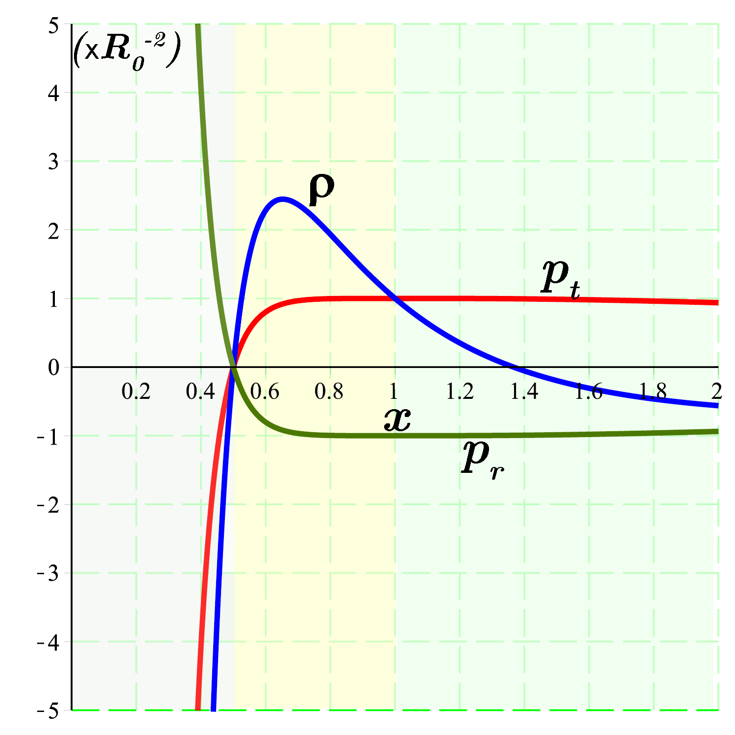
Figure 2: Plots of scaled $\rho,p_{r}$ and $p_{t}$ in terms of $x=\frac{R}{R_{0}}.$ The negative radial pressure outside the horizon is in analogy with the RW closed universe.

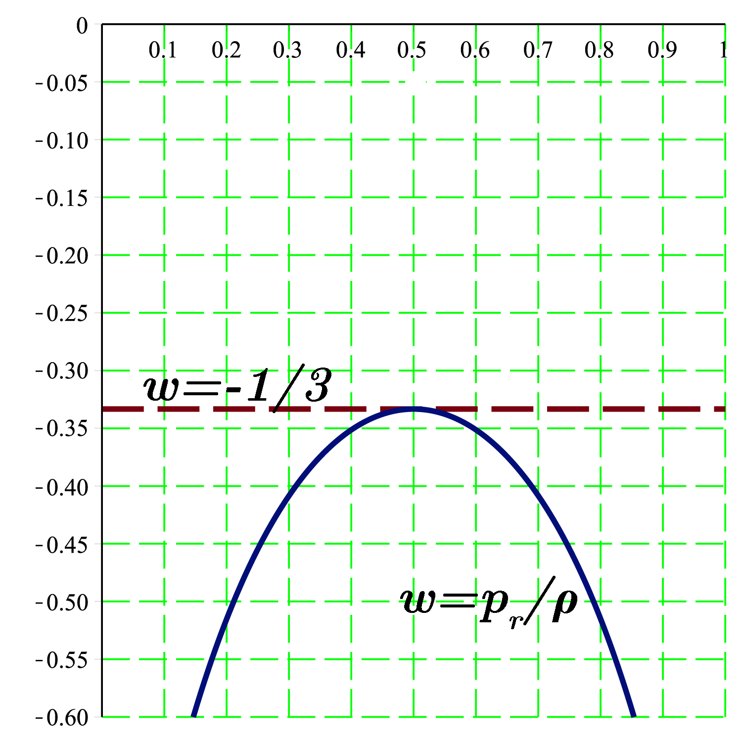
Figure 3: Plot $w=\frac{p_{r}}{\rho}$ in terms of $x=\frac{R}{R_{0}}.$ Near the horizon, it approaches $-\frac{1}{3}$ which is the same as the static RW closed universe.

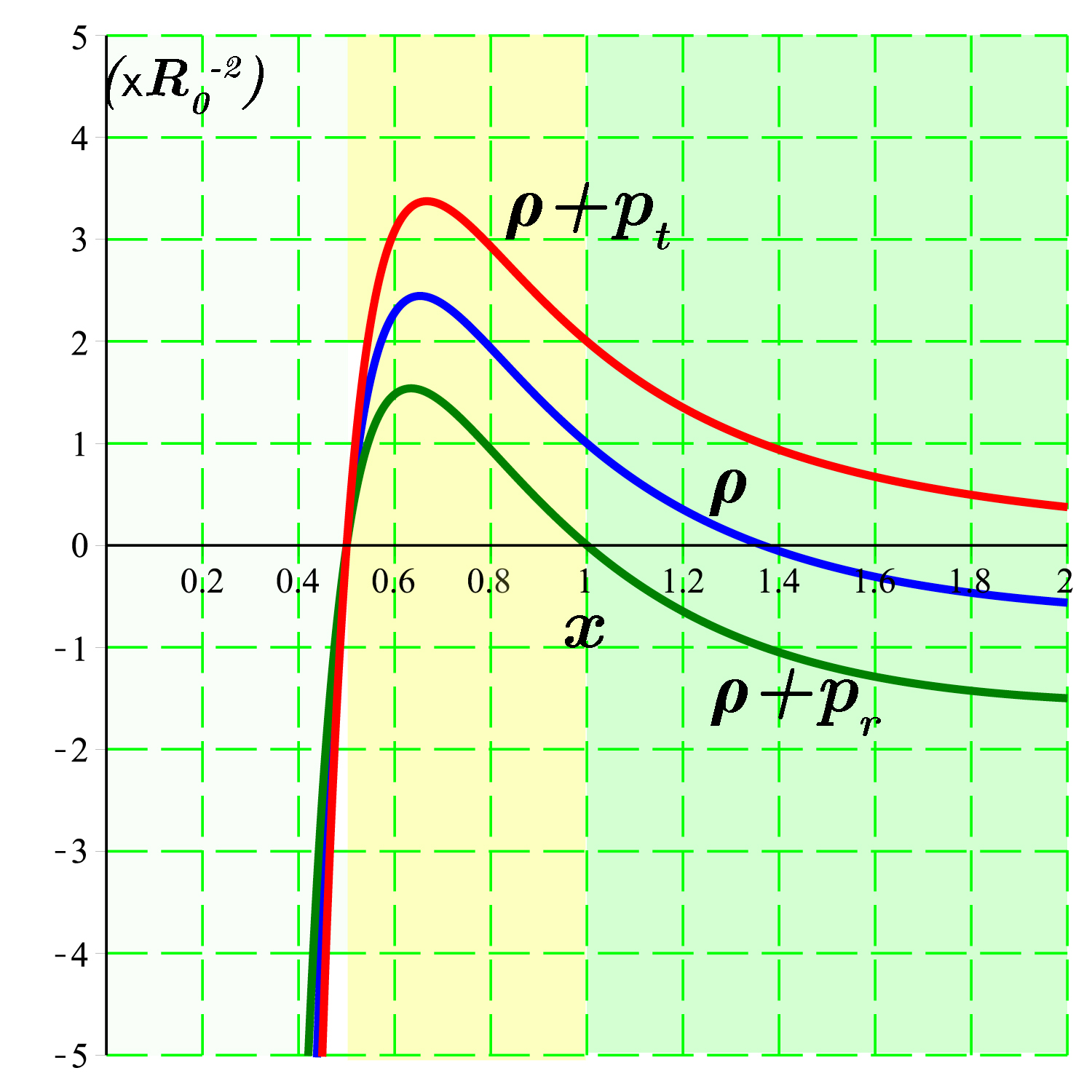
Figure 4: Plots of scaled $\rho,\rho+p_{r}$ and $\rho+p_{t}$ in terms of $x=\frac{R}{R_{0}}.$ While all of them are positive outside the horizon within the boundary of the universe at $x=1$, beyond this boundary we observe $\rho+p_{r}<0$, which implies that all energy conditions are violated and therefore the fluid is exotic.

In 25 where the black hole solution (11) has been introduced, it was claimed that this black hole is closed in 3-space or equivalently, it is formed in the $S_{3}$ background spatial topology. Such a black hole is known in the literature (see for instance 28 ; 29 ; 30 ; 31 ; 32 ; 33 ). To understand this feature we would like to make some investigation through the black holes which have been considered in this category (in particular, we refer to section 3.1 of Ref. 31 ). To do so we again start with the static cosmological model expressed by (3) which is actually a pure $S_{3}$ space topology solution. With $a\left(t\right)=1$ the spatial part becomes

$$ds_{3}^{2}=\frac{dR^{2}}{1-KR^{2}}+R^{2}\left(d\theta^{2}+\sin^{2}\theta d\varphi^{2}\right)$$ (20)

which after introducing $R=\frac{R_{0}}{\sqrt{K}}\sin\chi$ it becomes

$$ds_{3}^{2}=\frac{1}{K}R_{0}^{2}\left(d\chi^{2}+\sin^{2}\chi\left(d\theta^{2}+\sin^{2}\theta d\varphi^{2}\right)\right)$$ (21)

with the trivial topology of $S_{3}.$ We note that (21) possesses the $S_{3}$ space topology for all values of $\chi\in\left[0,\pi\right]$ and that is the reason it is pure $S_{3}$ with the geometry of 3-sphere.

In addition to the static RW spacetime which is the solution of Einstein’s equation supported by an isotropic, homogeneous, and uniform perfect fluid with the energy-momentum tensor governed by the EoS given by (5), there are black hole solutions 28 ; 29 ; 30 ; 31 ; 32 ; 33 which are supported by non-uniform perfect fluid with an EoS given by

$$p\left(r\right)=-\frac{\rho\left(r\right)}{3}.$$ (22)

One such solution was introduced by Bronnikov and Zaslavskii in 28 and can be described by the line element

$$ds^{2}=-\left(1-k\cot\chi\right)dt^{2}+\frac{R_{0}^{2}}{\left(1-k\cot\chi\right)}d\chi^{2}+R_{0}^{2}\sin^{2}\chi\left(d\theta^{2}+\sin^{2}\theta d\varphi^{2}\right)$$ (23)

in which $k$ and $R_{0}$ are two constants and $0\leq\chi\leq\pi.$ It is a black hole solution powered by the non-uniform perfect fluid with the energy-momentum tensor given by

$$T_{\mu}^{\nu}=\frac{3k\cot\chi-\sin\chi}{R_{0}^{2}\sin\chi}diag\left(1,-\frac{1}{3},-\frac{1}{3},-\frac{1}{3}\right).$$ (24)

The energy-momentum tensor satisfies the EoS (22), whereas the topology of the black hole (23) is not pure $S_{3}.$ However, in the vicinity of $\chi=\frac{\pi}{2},$ the spatial part of the spacetime becomes

$$ds_{3}^{2}\simeq R_{0}^{2}\left(d\chi^{2}+\sin^{2}\chi\left(d\theta^{2}+\sin^{2}\theta d\varphi^{2}\right)\right)$$ (25)

which reveals the $S_{3}$ space topology. We note that the geometry of the spatial part of (23) away from $\chi=\frac{\pi}{2}$ is nontrivial. In such a configuration, the spacetime is interpreted to be ”formed in the $S_{3}$ background spatial topology” (see 31 for more details).

Regarding the black hole solution subjected in this study i.e., the line element (12), by introducing $\frac{r}{r+r_{h}}=\sin\chi$ the spatial segment transforms into

$$ds_{3}^{2}=\frac{R_{0}^{2}\sin^{2}\left(2\chi\right)d\chi^{2}}{4\left(1-\sin\chi\right)^{2}\left(2\sin\chi-1\right)}+R_{0}{}^{2}\sin^{2}\chi d\Omega^{2}$$ (26)

in which $0\leq\chi\leq\frac{\pi}{2}$ and the horizon is located at $\chi=\frac{\pi}{6}.$ With this setting the geometry of the spacetime is still nontrivial although in the vicinity of $\chi\simeq\frac{14835\pi}{65536},$ (26) approximately becomes

$$ds_{3}^{2}\simeq R_{0}^{2}\left(\left(1+\zeta^{2}\right)d\chi^{2}+\sin^{2}\chi d\Omega^{2}\right)$$ (27)

which reveals the $S_{3}$ space topology of the spacetime near $\chi\simeq\frac{14835\pi}{65536}$ with a correction $\zeta^{2}\simeq 5.6379.$ In Fig. 1, we plot the scaled transformed metric function i.e., $\frac{R_{0}^{2}}{r_{h}^{2}}f\left(\chi\right),$ as well as $\frac{1}{R_{0}^{2}}g_{\chi\chi}$ from (27) and $\sin\chi$ for $0\leq\chi\leq\frac{\pi}{2}.$ It is observed that $\frac{1}{R_{0}^{2}}g_{\chi\chi}$ around its minimum i.e., $\chi\simeq\frac{14835\pi}{65536}$ is almost constant.

To get a better idea of the topology of the black hole spacetime (11) let us transform the spacetime into a more familiar system of coordinates. To do so, we introduce the following transformation

$$R\left(r\right)=R_{0}\left(\frac{r}{r+r_{h}}\right)=R$$ (28)

upon which the line element (11) becomes

$$ds^{2}=-f\left(R\right)dt^{2}+\frac{dR^{2}}{h\left(R\right)}+R^{2}d\Omega^{2}$$ (29)

in which

$$f\left(R\right)=\frac{2r_{h}R_{0}\left(R-R_{0}/2\right)}{R^{2}\left(R_{0}-R\right)^{2}}$$ (30)

and

$$h\left(R\right)=\frac{2\left(R_{0}-R\right)^{2}\left(R-R_{0}/2\right)}{R_{0}R^{2}}.$$ (31)

We note that, since $r\in\left[0,\infty\right),$ (28) implies $R\in\left[0,R_{0}\right)$ and indeed $t\in\left(-\infty,\infty\right)$ remains unchanged. Clearly (29) is a black hole with an event horizon located at $R=R_{+}=\frac{R_{0}}{2}.$ One can show that the Ricci and the Kretschmann scalars are respectively given by

$$\mathcal{R}=\frac{4\left(2R-R_{0}\right)\left(R_{0}-R\right)}{RR^{3}}$$ (32)

and

$$\mathcal{K}=\frac{8\left(30R^{6}-120R^{5}R_{0}+214R^{4}R_{0}^{2}-216R^{3}R_{0}^{3}+132R^{2}R_{0}^{4}-46RR_{0}^{5}+7R_{0}^{6}\right)}{R^{8}R_{0}^{2}}$$ (33)

which imply that the black hole is singular at $R=0$ and the Ricci scalar is positive outside the horizon. Let us add also that although the signature of the spacetime doesn’t change even with $R>R_{0}$ which indicates (29) is physically valid even for $R>R_{0}$, the scalar field $\psi$ transforms into

$$\psi\left(R\right)=\pm 2\sqrt{2}\arctan\left(\sqrt{\frac{R}{R_{0}-R}}\right)$$ (34)

which obviously is a pure imaginary function. This in turn indicates that the nature of the scalar field $\psi\left(R\right)$ changes into a phantom field. Similar to the RW universe (1), we apply Einstein’s equation for the black hole metric i.e. (29) to obtain

$$T_{\mu}^{\nu}=G_{\mu}^{\nu}=\left(-\rho,p_{r},p_{t},p_{t}\right)$$ (35)

in which the energy density $\rho,$ the radial pressure $p_{r},$ and the transverse pressure $p_{t}$ are, respectively, given by

$$\rho=\frac{6x^{2}-4x^{3}-1}{R_{0}^{2}x^{4}},$$ (36)

$$p_{r}=\frac{6x^{2}-4x^{3}-4x+1}{R_{0}^{2}x^{4}}$$ (37)

and

$$p_{t}=\frac{\left(2x-1\right)\left(2x^{2}-2x+1\right)}{R_{0}^{2}x^{4}}$$ (38)

in which $x=\frac{R}{R_{0}}.$ In Fig. 2, we plot $\rho$, $p_{r}$ and $p_{t}$ (all scaled by $R_{0}^{2}$) in terms of $x.$ It is observed that at the horizon they all vanish and near the horizon, the EoS approaches $p_{r}=-\frac{1}{3}\rho.$ This can be seen in Fig. 3 where we plot $w=\frac{p_{r}}{\rho}$ in terms of $x$ near the horizon. A similar EoS was already observed in the static RW universe in Eq. (5). Moreover, the radial pressure is negative outside the horizon which is in analogy with the RW closed universe. In Fig. 4, we plot also $\rho$, $\rho+p_{r}$ and $\rho+p_{t}$ (all are scaled by $R_{0}^{2}$) in terms of $x$. It is observed that since $\rho+p_{r}$ is negative for $x>1$ (outside the boundary of the universe) non of the energy conditions are satisfied. This implicitly implies that the physical region is located only within $x<1.$

III.1 Causal structure

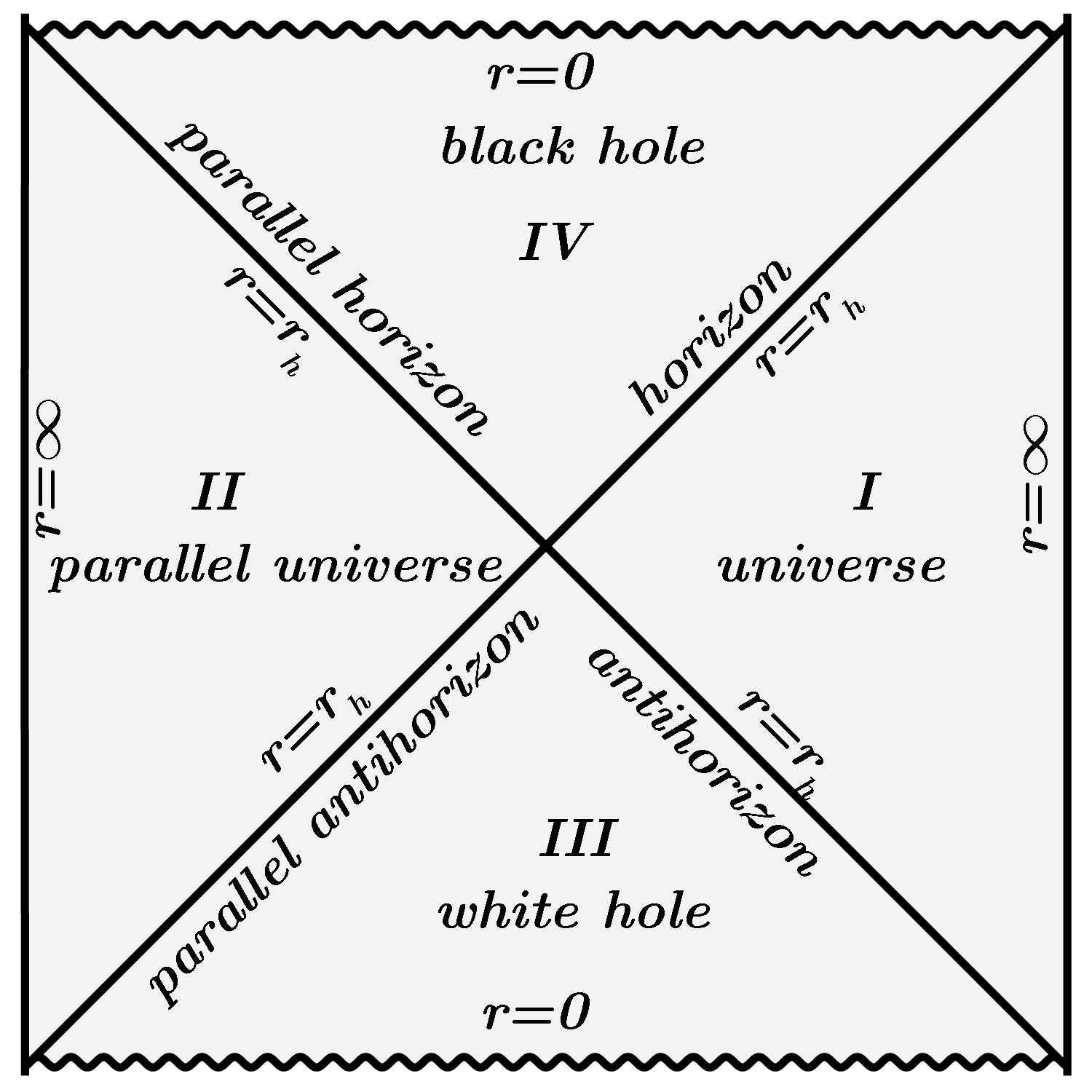
Figure 5: Penrose diagram of the black hole spacetime, given in (11). The spacetime singularity is spacelike and is located at $r=0$. Different regions are labeled appropriately on the figure.

To obtain the causal structure of the spacetime, we start from the original line element given in (11) and obtain the tortoise coordinate ($r>r_{h}$)

$$r_{\ast}=\int\sqrt{-\frac{g_{rr}}{g_{tt}}}dr=\int\frac{dr}{f\left(r\right)}=-\frac{R_{0}^{2}}{8r_{h}}\left[\frac{2r_{h}\left(3r+2r_{h}\right)}{\left(r+r_{h}\right)^{2}}+\ln\left|\frac{r+r_{h}}{r-r_{h}}\right|\right],$$ (39)

in which while $r\in\left(r_{h},\infty\right)$, $r_{\ast}\in\left(-\infty,0\right).$ Introducing the null coordinates i.e., $u=t-r_{\ast}$ and $v=t+r_{\ast}$ yields

$$ds^{2}=-\frac{\left(r+r_{h}\right){}^{3}\left(r-r_{h}\right)}{R_{0}^{2}r^{2}}dudv+R\left(r\right){}^{2}d\Omega^{2}$$ (40)

where $r=r\left(u,v\right).$ Now, we employ the Kruskal-Szekeres coordinates defined by

$$U=-\frac{R_{0}^{2}}{4r_{h}}e^{-\frac{4r_{h}}{R_{0}^{2}}u}$$ (41)

and

$$V=\frac{R_{0}^{2}}{4r_{h}}e^{\frac{4r_{h}}{R_{0}^{2}}v}$$ (42)

such that the line element (40) transforms into the following regular (at the horizon) form

$$ds^{2}=-\frac{\left(r+r_{h}\right){}^{4}e^{\frac{2r_{h}\left(3r+2r_{h}\right)}{\left(r+r_{h}\right)^{2}}}}{R_{0}^{2}r^{2}}dUdV+R\left(r\right){}^{2}d\Omega^{2}.$$ (43)

The line element (43) is regular everywhere except at the origin i.e., $r=0,$ and is valid for the entire region of $r>0$. From (41) and (42), one finds

$$UV=-\left(\frac{R_{0}^{2}}{4r_{h}}\right)^{2}e^{\frac{8r_{h}}{R_{0}^{2}}r_{\ast}}=-2\left(\frac{R_{0}^{2}}{4r_{h}}\right)^{2}\frac{r-r_{h}}{r+r_{h}}e^{-\frac{2r_{h}\left(3r+2r_{h}\right)}{\left(r+r_{h}\right)^{2}}},$$ (44)

and

$$\frac{V}{U}=e^{\frac{8r_{h}}{R_{0}^{2}}\left(\frac{v+w}{2}\right)}=e^{\frac{8r_{h}}{R_{0}^{2}}t},$$

which help us to understand the nature of spacetime not only outside the black hole but also inside. Eq. (39) implies that at the horizon where $r=r_{h},$ $r_{\ast}\rightarrow-\infty$ and $UV=0$. On the other hand when $r\rightarrow\infty$, $r_{\ast}=0$ which implies $UV=-\left(\frac{R_{0}^{2}}{4r_{h}}\right)^{2}<0$ which is a constant. More interestingly, with $r\rightarrow 0$, $UV=2\left(\frac{R_{0}^{2}}{4er_{h}}\right)^{2}>0$ which is also a constant implying the singularity is spacelike. Based on the above calculations in Fig. 5, we plot the Penrose diagram of the black hole spacetime (11). It shows that the topology of the asymptotic regions i.e., $I$ and $II$ is $AdS_{2}\times S^{2}$, however, the radius of the round 2-sphere at a point of radius $r$ is not equal to $r$ but $R\left(r\right),$ given in (13). Moreover, the topology of the interior region i.e., $III$ and $IV$ which are the future black hole and the past black hole (or white hole) is $\mathbb{R}\times\mathbb{R}\times S^{2}$ such that the radius of $S^{2}$ is again $R\left(r\right)$. We also noted in Fig. 5 the boundaries in terms of the transformed coordinates in (29). It is clear that the black hole is bounded by a timelike hypersurface located at $R=R_{0}.$ In this regard, the radius of the 2-sphere corresponding to each point of radius $R$ is exactly $R.$

IV Trajectories of particles

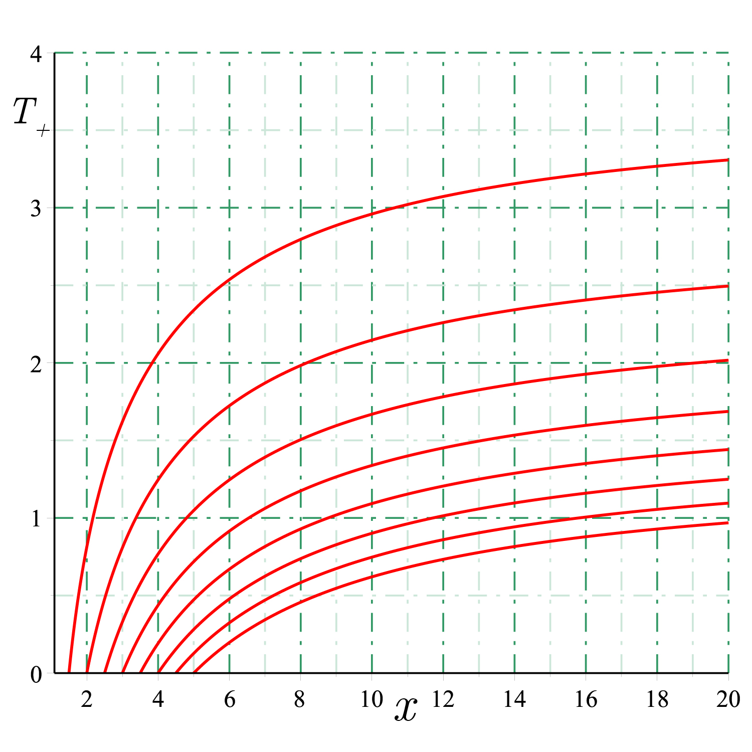
Figure 6: The plots of $T_{+}$ in terms of $x$, from Eq. (59) for $x_{0}=1.5,2.0,...,5$ with equal steps.

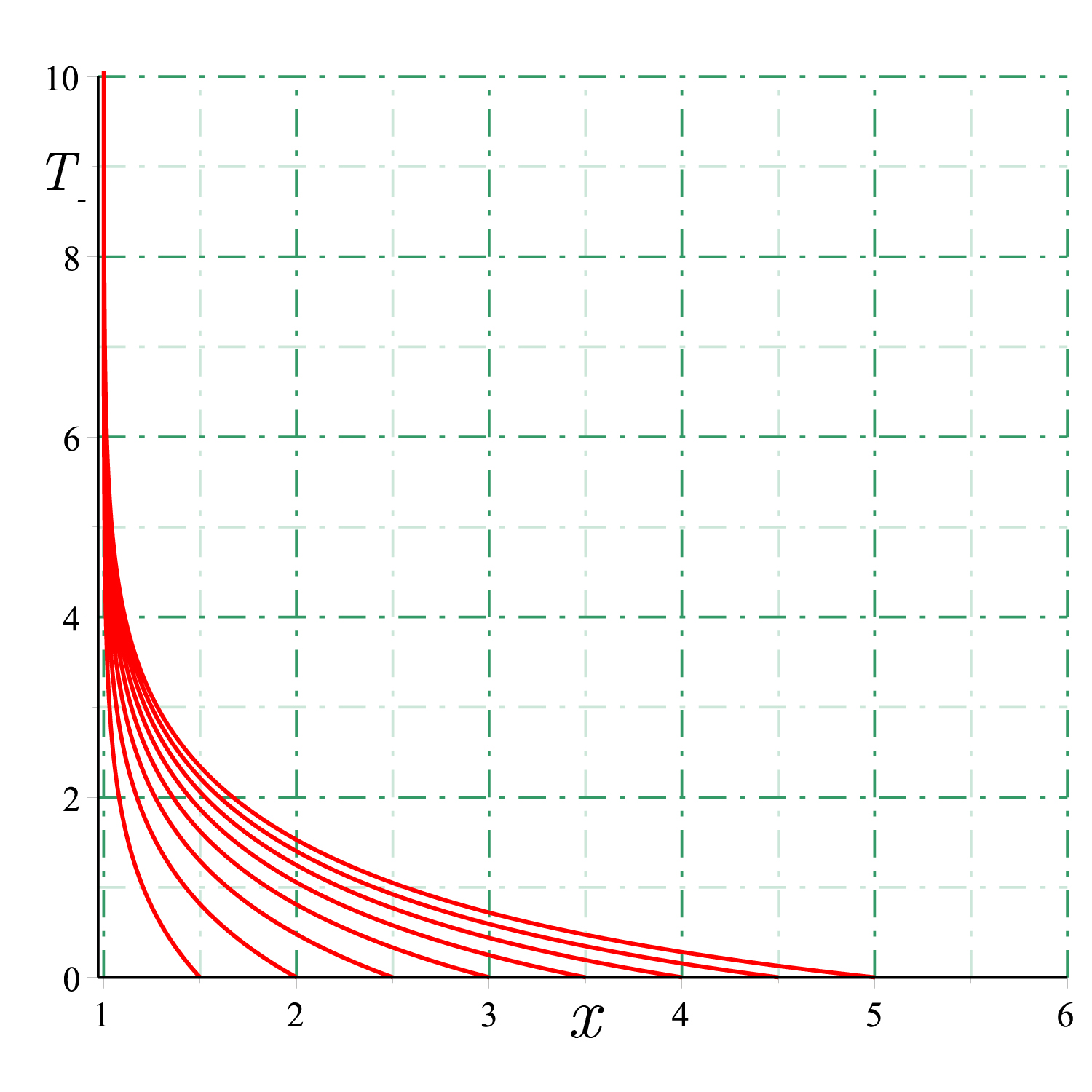
Figure 7: The plots of $T_{-}$ in terms of $x$, from Eq. (59) for $x_{0}=1.5,2.0,...,5$ with equal steps.

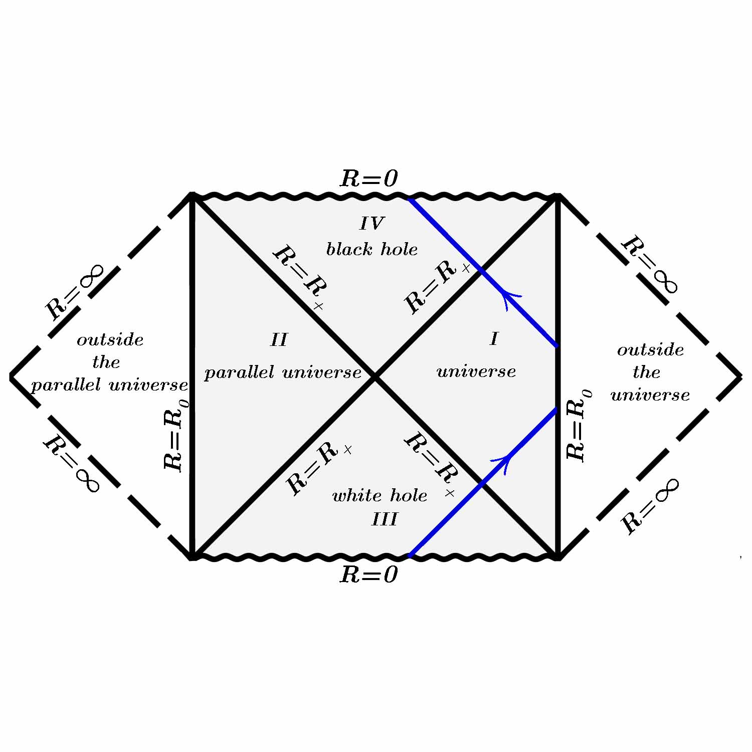
Figure 8: The Penrose diagram of the black hole in the transformed coordinates ($t,R,\theta,\varphi$). The universe which is supported by physical fields is shaded. The light beam can not reach outside regions which are not physical.

In this section, we study the geodesics of particles in the spacetime of the black hole introduced in Ref. 25 . Precisely, we investigate the radial and circular time-like and null geodesics of test particles. The static spherically symmetric black hole found in Ref. 25 is described by the line element (11) where the two metric functions are given by (11) and (12) in which $r\in\left[0,\infty\right),$ $R_{0}$ is a real constant and $r_{h}$ is the radius of the event horizon. The Lagrangian of a massive particle with a unit mass is described by $\mathcal{L}=\frac{1}{2}g_{\mu\nu}\dot{x}^{\mu}\dot{x}^{\nu}$ which explicitly reads

$$\mathcal{L}=\frac{1}{2}\left(-f\left(r\right)\dot{t}^{2}+\frac{r^{2}}{f\left(r\right)}+R\left(r\right){}^{2}\left(\dot{\theta}^{2}+\sin^{2}\theta\dot{\phi}^{2}\right)\right)$$ (45)

in which a dot indicates a derivative with respect to an affine parameter (here $\lambda$) for massless particles and the proper time for massive particles. The Lagrangian (45) is independent of time $t$ and azimuthal angle $\phi$ which results in two conserved quantities: 1) the energy $E=-\frac{\partial\mathcal{L}}{\partial\dot{t}}$ and 2) the angular momentum in $\phi$ direction $\ell=\frac{\partial\mathcal{L}}{\partial\dot{\phi}}$. Therefore, one writes

$$E=\,f\left(r\right)\frac{dt}{d\lambda}$$ (46)

and

$$\ell=\,R\left(r\right)^{2}\sin^{2}\theta\frac{d\phi}{d\lambda}$$ (47)

which are both conserved. Since we are interested in the geodesics on the equatorial plane where $\theta\,=\,\frac{\pi}{2}$, the angular momentum reduces to

$$\ell=R\left(r\right){}^{2}\frac{d\phi}{d\lambda}.$$ (48)

Furthermore, considering the definition of the four-velocity $U^{\mu}=\frac{dx^{\mu}}{d\lambda}$ that satisfies $U^{\mu}U_{\mu}=-\epsilon$ in which $\epsilon=+1,-1,$ and $0$ for timelike, spacelike, and null particles, we explicitly obtain the condition

$$g_{\mu\nu}\frac{dx^{\mu}}{d\lambda}\frac{dx^{\nu}}{d\lambda}=-\epsilon.$$ (49)

Upon combining Eqs. (46), (47) and (49), after setting $\theta\,=\,\frac{\pi}{2},$ we determine

$$\left(\frac{dr}{d\lambda}\right)^{2}=E^{2}-f\left(r\right)\left(\epsilon+\frac{\ell^{2}}{R(r)^{2}}\right)$$ (50)

which is the geodesic equation for the radial coordinate $r.$ In addition, by introducing an effective potential in the form $V_{eff}^{2}\left(r\right)\,=\,\frac{1}{2}f\left(r\right)\left(\epsilon+\frac{\ell^{2}}{R(r)^{2}}\right)$ and an effective energy $\varepsilon_{eff}^{2}\,=\,\frac{1}{2}E^{2}$, the radial geodesics equation is given in a more familiar form of an equation of motion for a test particle with unit mass, i.e.,

$$\frac{1}{2}\left(\frac{du}{d\lambda}\right)^{2}+V_{eff}^{2}\left(r\right)=\mathcal{E}_{eff}^{2}.$$ (51)

The exact form of the effective potential by replacing $f(r)$ from Eq. (12) is expressed by

$$V_{eff}^{2}\left(r\right)=\frac{1}{2}\frac{\left(r+r_{h}\right){}^{2}\left(r^{2}-r_{h}^{2}\right)}{R_{0}^{2}r^{2}}\left(\epsilon+\frac{\ell^{2}\left(r+r_{h}\right)^{2}}{R_{0}^{2}r^{2}}\right).$$ (52)

Let us note that, from Eq. (51) to have $r$ a real coordinate, the condition $\mathcal{E}_{eff}^{2}\geq V_{eff}^{2}\left(r\right)$ should hold. Moreover, by applying the chain rule $\frac{dr}{d\lambda}\,=\,\frac{dr}{d\phi}\frac{d\phi}{d\lambda}$, one eliminates the affine parameter from the main geodesic equation to get

$$\left(\frac{dr}{d\phi}\right)^{2}=\frac{2R\left(r\right){}^{4}}{\ell^{2}}\left(\mathcal{E}_{eff}^{2}-V_{eff}^{2}\left(r\right)\right).$$ (53)

The latter equation explicitly reads

$$\left(\frac{dr}{d\phi}\right)^{2}=\frac{E^{2}}{\ell^{2}}R\left(r\right){}^{4}-f\left(r\right)\left(\epsilon\frac{R(r)^{4}}{\ell^{2}}+R(r)^{2}\right)\,:=\,G\left(r\right)$$ (54)

in which the right-hand side has to satisfy $G\left(r\right)\geq 0$. In what follows we classify the geodesics in different cases.

IV.1 Radial Motion

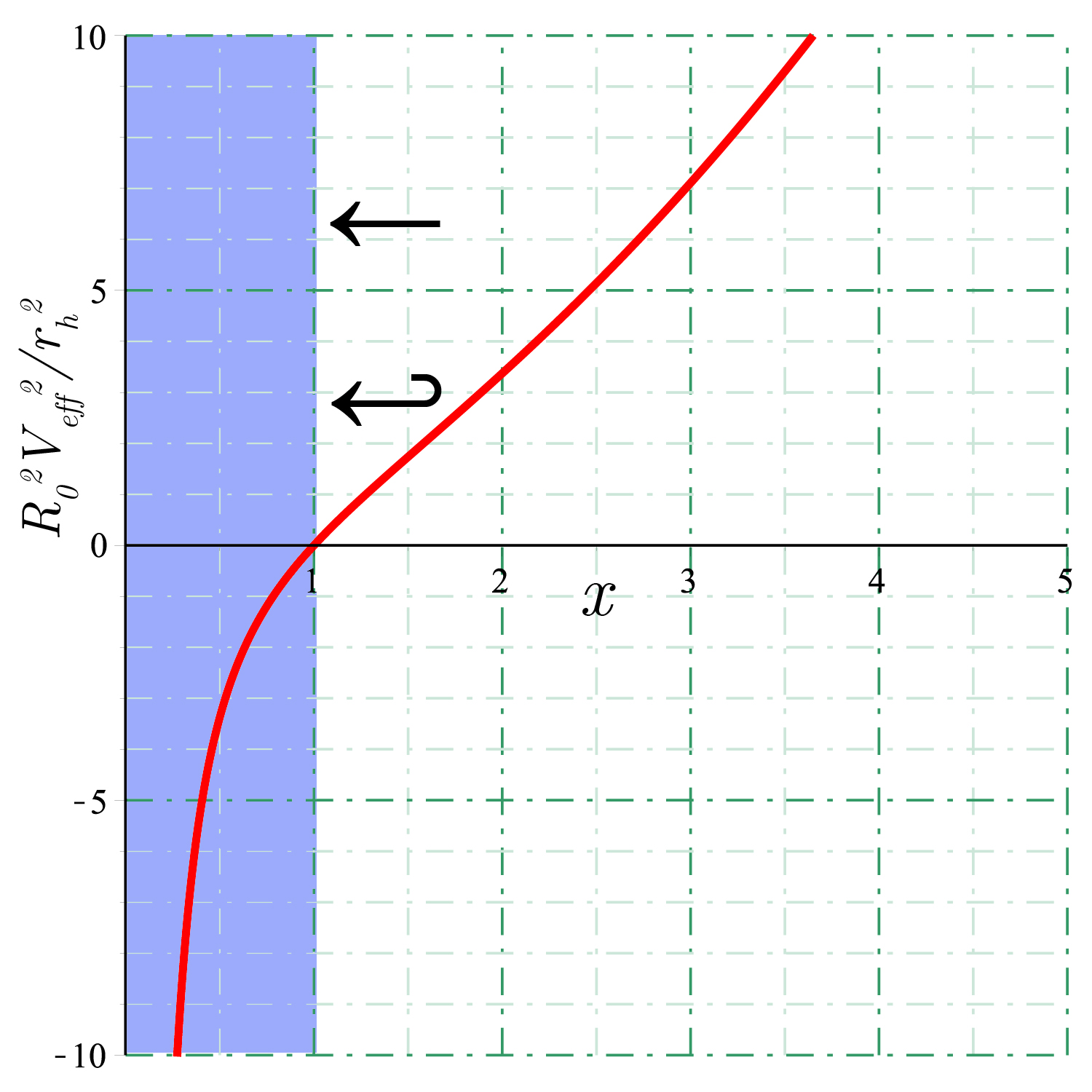
Figure 9: The generic plot of $\frac{R_{0}^{2}}{u_{h}}V_{eff}^{2}\left(r\right)$ in terms of $x=\frac{r}{r_{h}}.$ The shaded region implies inside the black hole and the horizon is at $x=1.$ The massive particle in its radial motion has no chance to escape to the edge of spacetime. This means that the massive timelike particle either directly collapses to the singularity of the spacetime or after it bounces from the potential barrier, as shown in the figure.

For a radial motion the angular momentum has to be zero i.e., $\ell\,=\,0$, upon which (47) yields $\phi\,=\,const.$ such that the particle will move radially. Hence, Eq. (50) reduces to

$$\left(\frac{dr}{d\lambda}\right)^{2}=E^{2}-\epsilon f\left(r\right)$$ (55)

In the following subsections, we shall investigate null and time-like geodesics for radial motion separately.

IV.1.1 Null geodesics $\epsilon\,=\,0$

Considering $\epsilon\,=\,0$ in (55) for the null geodesics which describes the motion of a massless particle (photon), we simply find

$$\left(\frac{dr}{d\lambda}\right)^{2}=E^{2}$$ (56)

which simply shows that the radial outgoing null geodesics are future-complete. On the other hand combining (46) and (56), we get,

$$\frac{dr}{dt}=\pm f\left(r\right)\,=\,\pm\frac{\left(r+r_{h}\right){}^{2}\left(r^{2}-r_{h}^{2}\right)}{R_{0}^{2}r^{2}}.$$ (57)

Eq. (57) is integrable and explicitly yields the following

$$\frac{R_{0}^{2}}{4}\left(\frac{1}{2r_{h}}\ln\left[\frac{\left(r-r_{h}\right)\left(r_{0}+r_{h}\right)}{\left(r+r_{h}\right)\left(r_{0}-r_{h}\right)}\right]-\frac{3r+2r_{h}}{\left(r+r_{h}\right){}^{2}}+\frac{3r_{0}+2r_{h}}{\left(r_{0}+r_{h}\right){}^{2}}\right)=\pm\left(t-t_{0}\right)$$ (58)

where $t_{0}$ is the initial time, $t$ is the time measured by the distant observer and $r_{0}$ is the initial position of the massless particle (photon). Introducing $r=r_{h}x$, $r_{0}=r_{h}x_{0}$ and $T=\frac{8r_{h}}{R_{0}^{2}}\left(t-t_{0}\right)$ we obtain

$$T_{\pm}=\pm\left(\ln\left[\frac{\left(x-1\right)\left(x_{0}+1\right)}{\left(x+1\right)\left(x_{0}-1\right)}\right]-2\frac{3x+2}{\left(x+1\right){}^{2}}+2\frac{3x_{0}+2}{\left(x_{0}+1\right){}^{2}}\right).$$ (59)

We note that $\pm$ refers to the outgoing or ingoing light rays. In Fig. 6 we plot $T_{+}$ in terms of $x$ for various values of $x_{0}.$ From this figure, we observe that on the equilateral plane, the photon moves away from the horizon toward the boundary of the spacetime where $r\rightarrow\infty.$ The time needed for the photon to reach the boundary of the spacetime is found to be

$$T_{+\infty}=2\frac{3x_{0}+2}{\left(x_{0}+1\right){}^{2}}+\ln\frac{x_{0}+1}{x_{0}-1}$$ (60)

which is finite. Furthermore, in Fig. 7 we plot $T$ in terms of $x$ for various values of $x_{0}$. We see that with initial velocity toward the horizon, the photon to reach the horizon at an infinite time measured by a distant observer.

IV.1.2 Null geodesics in the transformed coordinates

In this part, we would like to present the radial motion of null particles namely photons in the vicinity of the black hole described by the transformed coordinate given in Eqs. (29)-(31). Similar calculations reveal that the transformed version of the radial equation for a null particle i.e., Eq. (56) becomes

$$\left(\frac{dR}{d\lambda}\right)^{2}=\frac{h\left(R\right)}{f\left(R\right)}E^{2}.$$ (61)

This equation explicitly reads as

$$\frac{dR}{d\lambda}=\pm\frac{\left|E\right|}{u_{h}R_{0}}\left(R_{0}-R\right)^{2}$$ (62)

in which $\pm$ stand for the outgoing ($+$) and ingoing ($-$) null beam. Assuming the initial position of the null beam to be $R=R_{i}$ at $\lambda=\lambda_{i},$ the latter equation admits exact solutions given by

$$R_{\pm}=R_{0}-\frac{1}{\frac{1}{R_{0}-R_{i}}\pm\frac{\left|E\right|}{u_{h}R_{0}}\left(\lambda-\lambda_{i}\right)}.$$ (63)

One can easily check that $\lim_{\lambda\rightarrow\lambda_{i}}R_{\pm}=R_{i}$, while

$$\lim_{\lambda\rightarrow\infty}R_{+}=R_{0},$$ (64)

which implies that null particles cannot pass the boundary at $R=R_{0}.$ On the other hand, (63) yields the interval of $\lambda$ which is needed for the ingoing beam reaches to the event horizon given by

$$\triangle\lambda=\frac{u_{h}R_{0}}{\left|E\right|}\left(\frac{1}{R_{0}-R_{i}}-\frac{2}{R_{0}}\right).$$ (65)

This shows that the maximum $\triangle\lambda\rightarrow\infty$ when $R_{i}\rightarrow R_{0}$ when the light beam is directed toward the black hole from the edge of the universe. For any other initial position, $\triangle\lambda$ is a finite positive number. In Fig. 8, we plot the Penrose diagram of the black hole in the transformed coordinates with the line element (29). As expected the Penrose diagram is the same as Fig. 5 and the only difference is the boundary of the universe. Furthermore, in Fig. 8 we have shown the excluded regions i.e., $R>R_{0}$ which corresponds to the phantom scalar field and the light ray can not reach there. The blue rays stand for the null geodesics.

IV.1.3 Time-like geodesics $\epsilon\,=\,1$

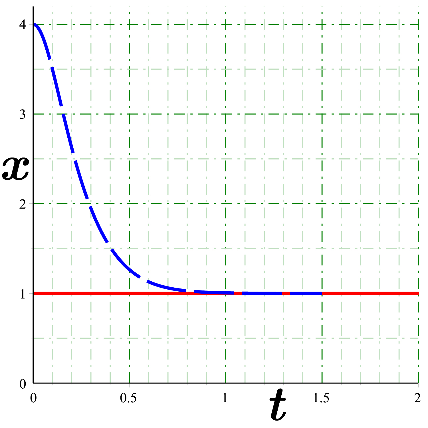
Figure 10: The radial motion of a massive particle (dashed-blue curve) with $\tilde{R}_{0}=1,\left(\frac{dx}{dt}\right)_{t=0}=0$ and $\tilde{E}^{2}=\frac{375}{16}$. The horizon is located at $x=1$ (red solid line). This is the numeric plot of the radial geodesic equation (75) constraint by (74).

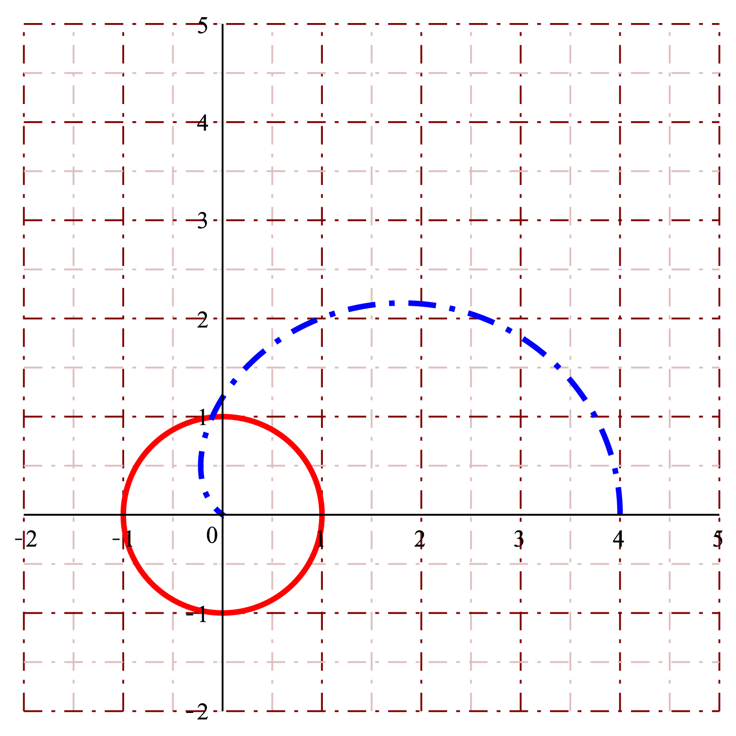
Figure 11: Trajectory of a photon (dashed-blue curve) with $\tilde{\ell}^{2}=2,\left(\frac{dx}{d\varphi}\right)_{\varphi=0}=0$ and $\tilde{E}^{2}=\frac{9375}{128}$. The horizon is located at $x=1$ (red circle).

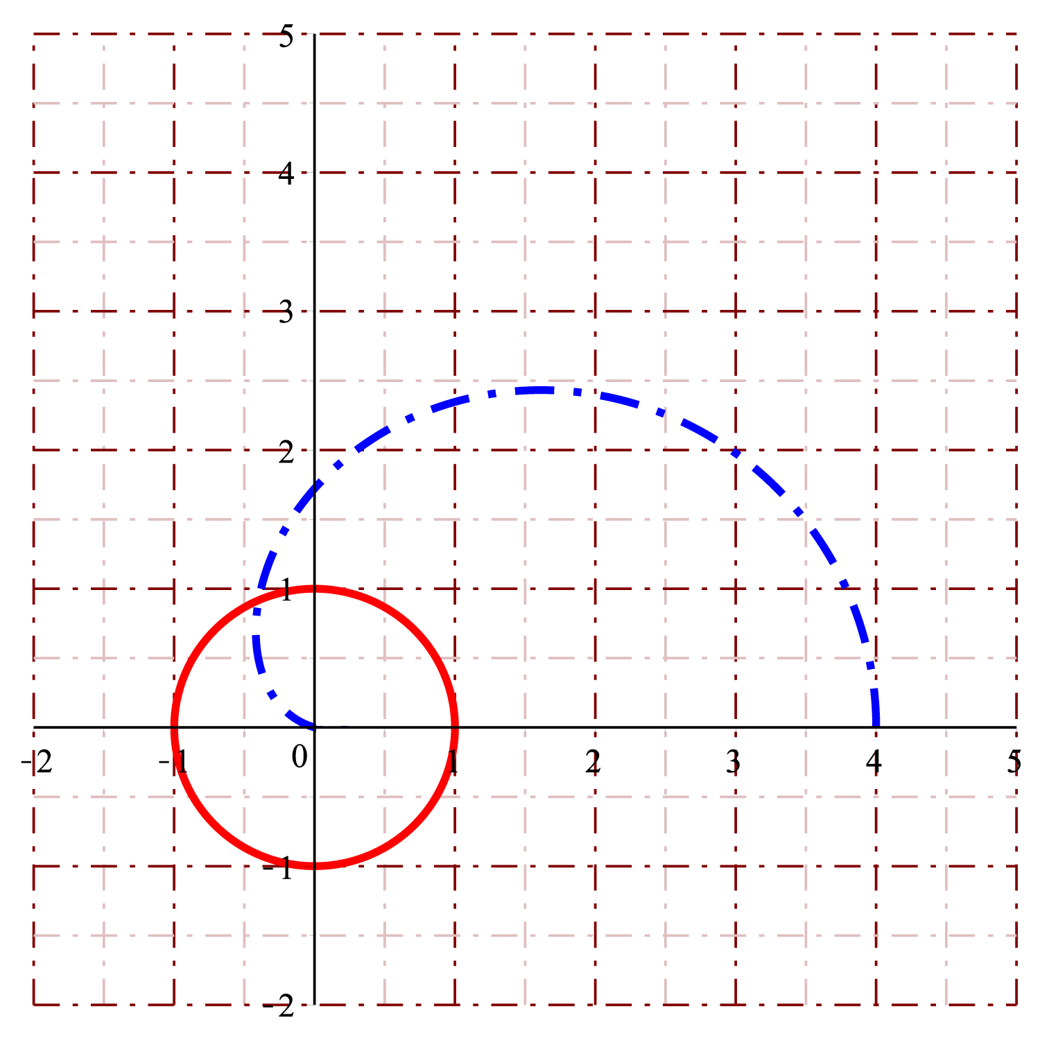
Figure 12: Trajectory of a timelike particle (dashed-blue curve) with $\tilde{\ell}^{2}=2,\left(\frac{dx}{d\varphi}\right)_{\varphi=0}=0$ and $\tilde{E}^{2}=\frac{12375}{128}$. The horizon is located at $x=1$ (red circle).

Time-like geodesics refers to the motion of a massive particle where $\epsilon\,=\,1$ upon which (55) becomes

$$\left(\frac{dr}{d\lambda}\right)^{2}=\,E^{2}-\frac{\left(r+r_{h}\right){}^{2}\left(r^{2}-r_{h}^{2}\right)}{R_{0}^{2}r^{2}}.$$ (66)

Derivative of (66) with respect to the affine parameter $\lambda$ implies

$$\frac{d^{2}r}{d\tau^{2}}=-\frac{1}{R_{0}^{2}r^{3}}\left(r+r_{h}\right)\left(r^{3}+r_{h}^{3}\right),$$ (67)

in which we set $\lambda=\tau$ where $\tau$ is the proper time. Obviously, the radial force per unit mass is attractive and toward the horizon of the black hole. We assume that the particle is initially at rest located at $r=r_{0}$ such that (66) yields

$$E^{2}=\frac{\left(r_{0}+r_{h}\right){}^{2}\left(r_{0}^{2}-r_{h}^{2}\right)}{R_{0}^{2}r_{0}^{2}}$$ (68)

upon which (66) becomes

$$\left(\frac{dr}{d\tau}\right)^{2}=\frac{1}{R_{0}^{2}}\left(\frac{\left(r_{0}+r_{h}\right){}^{2}\left(r_{0}^{2}-r_{h}^{2}\right)}{r_{0}^{2}}-\frac{\left(r+r_{h}\right){}^{2}\left(r^{2}-r_{h}^{2}\right)}{r^{2}}\right),$$ (69)

and with $\ell\,=\,0$ and $\epsilon\,=\,1$, the effective potential becomes

$$V_{eff}^{2}\left(r\right)=\frac{1}{2}\frac{\left(r+r_{h}\right){}^{2}\left(r^{2}-r_{h}^{2}\right)}{R_{0}^{2}r^{2}}.$$ (70)

In Fig. 9 we plotted $\frac{R_{0}^{2}}{r_{h}}V_{eff}^{2}\left(r\right)$ in terms of $x=\frac{r}{r_{h}}$ which shows that the potential is an increasing function implying an attractive force toward the singularity. Therefore no matter what is the energy of the particle, its fate is a collapse into the singularity. Finally, using Eqs. (66) and (46) we find the radial equation of motion of a massive particle in terms of the observer time i.e.,

$$\left(\frac{dr}{dt}\right)^{2}=f\left(r\right){}^{2}-\frac{f\left(r\right){}^{3}}{E^{2}}$$ (71)

and explicitly

$$\left(\frac{dr}{dt}\right)^{2}=\frac{\left(r+r_{h}\right){}^{4}\left(r^{2}-r_{h}^{2}\right){}^{2}}{R_{0}^{4}r^{4}}\left(1-\frac{\left(r+r_{h}\right){}^{2}\left(r^{2}-r_{h}^{2}\right)}{E^{2}R_{0}^{2}r^{2}}\right).$$ (72)

Considering the timelike particle is initially at rest where $r=r_{0}$, one writes

$$0=\frac{\left(r_{0}+r_{h}\right){}^{4}\left(r_{0}^{2}-r_{h}^{2}\right){}^{2}}{R_{0}^{4}r_{0}^{4}}\left(1-\frac{\left(r_{0}+r_{h}\right){}^{2}\left(r_{0}^{2}-r_{h}^{2}\right)}{E^{2}R_{0}^{2}r_{0}^{2}}\right)$$ (73)

which yields the conserved energy of the particle in terms of its initial position given in Eq. (68). Introducing $r\left(t\right)=x\left(t\right)r_{h}$, $R_{0}=\tilde{R}_{0}\sqrt{r_{h}}$ and $E=\tilde{E}\sqrt{r_{h}}$ we obtain the following equation

$$\left(\frac{dx}{dt}\right)^{2}=\frac{\left(x^{2}-1\right)^{2}\left(1+x\right)^{4}}{\tilde{R}_{0}^{4}x^{4}}-\frac{\left(x^{2}-1\right)^{3}\left(1+x\right)^{6}}{\tilde{R}_{0}^{6}\tilde{E}^{2}x^{6}}$$ (74)

and after differentiating with respect to $t$ the main differential equation is obtained

$$\frac{d^{2}x}{dt^{2}}=\frac{2\left(x^{2}-1\right)\left(1+x\right)^{4}\left(1-x+x^{2}\right)}{\tilde{R}_{0}^{4}x^{5}}-\frac{3\left(x^{2}-1\right)^{2}\left(1+x\right)^{6}\left(1-x+x^{2}\right)}{\tilde{R}_{0}^{6}\tilde{E}^{2}x^{7}}.$$ (75)

The latter equation is highly nonlinear and cannot be solved analytically. Therefore we solve it by applying the numerical method. In Fig. 10 we plotted $x\left(t\right)$ in terms of $t$ where the parameters are set to be $\tilde{R}_{0}=1$ and $\tilde{E}^{2}=\frac{375}{16}$ and the initial conditions are given by $x_{0}=4$ and $\left(\frac{dx}{dt}\right)_{0}=0.$

IV.2 General equatorial motion

Having known that a circular motion is not possible, in this section we study the general motion of null/timelike particles on the equatorial plane. The trajectory of such particles has to satisfy the following equations

$$\left(\frac{dx}{d\varphi}\right)^{2}=\epsilon\frac{\left(1-x\right)x^{2}}{\left(1+x\right)\tilde{\ell}^{2}}+\frac{\tilde{E}^{2}x^{4}}{\tilde{\ell}^{2}\left(1+x\right)^{4}}+\left(1-x^{2}\right)$$ (76)

and

$$\frac{d^{2}x}{d\varphi^{2}}=\epsilon\frac{\left(1-x-x^{2}\right)x}{\left(1+x\right)^{2}\tilde{\ell}^{2}}+\frac{2\tilde{E}^{2}x^{3}}{\tilde{\ell}^{2}\left(1+x\right)^{5}}-x$$ (77)

in which we have introduced $x\left(\varphi\right)=r\left(\varphi\right)/r_{h},$ $\tilde{\ell}^{2}=\ell^{2}/R_{0}^{2},$ and $\tilde{E}^{2}=R_{0}^{2}E^{2}/r_{h}^{2}.$ The nonlinear structure of the geodesics main equation (77) prevents obtaining an exact solution, however, we solved (77) using a numerical method, and the results are presented in Figs. 11 and 12 for the null ($\epsilon=0$) and the timelike ($\epsilon=1$) particles. It is observed that with nonzero angular momentum, no matter what the initial conditions are, the particle eventually falls into the black hole.

V Conclusion

This study sheds light on the physical properties of the black hole of Ref. 25 which is of a class of black holes formed in $S_{3}$ background spatial topology. In the $r$ coordinate, one can see from the line element (11) and the radial null geodesic equation (56) that the spacetime is not compact. This can also be seen in the Penrose diagram of the black hole solution in Figs. 5. However, the radius of the $S^{2}$ sphere corresponding to each point of spacetime of radius $r$ is $R\left(r\right)=R_{0}\frac{r}{r+r_{h}}$ that asymptotically goes to $R_{0}.$ With a proper transformation we have shown that in the transformed line element given in Eq. (26), the spatial part possesses an $S_{3}$ topology in the vicinity of $\chi\simeq\frac{14835\pi}{65536}$. Our new analysis in the transformed line element, particularly based on the radial null geodesics equation (62), shows that the light beam can not pass the timelike boundary of the black hole at $R=R_{0}.$ This is demonstrated in the second Penrose diagram in Fig. 8. In addition to that we studied the geodesics of the null and timelike particles. In the first part of our geodesics analysis, we studied the radial motion of a photon and a massive particle on the equatorial plane. For a photon, we observed that depending on the light beam’s direction, it may go to the edge of the universe in a finite time measured by a distant observer or it reaches the black hole in an infinite time. On the other hand, a massive timelike particle collapses to the singularity irrespective of the direction of its initial velocity. One can see from Fig. 10 that there is no stable circular orbit neither for a photon nor for a massive particle. We observed also that massive particles as well as non-radially outgoing light beams all are attracted by the black hole. Is this unusual or universal behavior of all black holes formed in $S_{3}$ background spatial topology? This question can not be answered here. A concrete answer needs further investigation on the geodesics of other black holes in the same class. We leave this problem open.

References

- (1) W. Israel, Event Horizons in Static Vacuum Space-Times. Phys. Rev. 164, 1776 (1967).
- (2) W. Israel, Event horizons in static electrovac space-times. Commun. Math. Phys. 8, 245 (1968).
- (3) B. Carter, Axisymmetric Black Hole Has Only Two Degrees of Freedom. Phys. Rev. Lett. 26, 331 (1971).
- (4) R. M. Wald, Final States of Gravitational Collapse. Phys. Rev. Lett. 26, 1653 (1971).
- (5) J. D. Bekenstein, Novel ”no-scalar-hair” theorem for black holes. Phys. Rev. D 51, R6608 (1995).
- (6) M. S. Volkov and D. V. Galtsov, Non Abelian Einstein Yang-Mills black holes. Pisma Zh. Eksp. Teor. Fiz. 50, 312 (1989).
- (7) P. Bizon, Colored black holes. Phys. Rev. Lett. 64, 2844 (1990).
- (8) B. R. Greene, S. D. Mathur and C. M. O’Neill, Eluding the no-hair conjecture: Black holes in spontaneously broken gauge theories. Phys. Rev. D 47, 2242 (1993).
- (9) P. Nicolini and E. Spallucci, Noncommutative geometry inspired dirty black holes. Class. Quantum Grav. 27, 015010 (2010).
- (10) T. J. Allen, M. J. Bowick and A. Lahiri, Axionic black holes from massive axions. Phys. Lett. B 237, 47 (1990).
- (11) B. A. Campbell, N. Kaloper and K. A. Olive, Axion hair for dyon black holes. Phys. Lett. B 263, 346 (1991).
- (12) K. Lee and E. J. Weinberg, Charged black holes with scalar hair. Phys. Rev. D 44, 3159 (1991).
- (13) G. W. Gibbons and K.I. Maeda, Black Holes and Membranes in Higher Dimensional Theories with Dilaton Fields. Nucl. Phys. B 298, 741 (1988).
- (14) I. Ichinose and H. Yamazaki, Charged Black Hole Solutions in Superstring Theory. Mod. Phys. Lett. A 4, 1509 (1989).
- (15) H. Yamazaki and I. Ichinose, Dilaton field and charged black hole. Class. Quntum Grav. 9, 257 (1992).
- (16) D. Garfinkle, G. T. Horowitz and A. Strominger, Charged black holes in string theory. Phys. Rev. D 43, 3140 (1991).
- (17) F. Dowker, R. Gregory and J. Traschen, Euclidean black-hole vortices. Phys. Rev D 45, 2762 (1992).
- (18) I. Z. Fisher, Scalar mesostatic field with regard for gravitational effects. Zh. Eksp. Teor. Fiz. 18, 636 (1948).
- (19) M. B. Green, J. H. Schwarz and E. Witten, 1987 Superstring Theory (Cambridge: Cambridge University Press).
- (20) B. Harms and Y. Leblanc, Statistical mechanics of black holes. Phys. Rev. D 46, 2334 (1992).
- (21) C. F. E. Holzhey and F. Wilczek, Black Holes as Elementary Particles. Nucl. Phys. B 380, 447 (1992).
- (22) G. W. Gibbons and K.-I. Maeda, Black Holes and Membranes in Higher Dimensional Theories with Dilaton Fields. Nucl. Phys. B 298, 741 (1988) .
- (23) D. Garfinkle, G. T. Horowitz and A. Strominger, Charged black holes in string theory. Phys. Rev. D 43, 3140 (1991).[ Erratum-ibid D 45, 3888 (1992)].
- (24) D. Brill and G. T. Horowitz, Negative energy in string theory. Phys. Lett. B 262, 437 (1991).
- (25) R. Gregory and J. A. Harvey, Black Holes with a Massive Dilaton. Phys. Rev. D 47, 2411 (1993).
- (26) T. Koikawa and M. Yoshimura, Dilaton fields and event horizon. Phys. Lett. B 189, 29 (1987) .
- (27) D. G. Boulware and S. Deser, Effective gravity theories with dilations. Phys. Lett. B 175, 409 (1986).
- (28) M. Rakhmanov, Dilaton black holes with electric charge. Phys. Rev. D 50, 5155 (1994).
- (29) K. C. K. Chan, J. H. Horn and R. B. Mann, Charged dilaton black holes with unusual asymptotics. Nucl. Phys. B 447, 441 (1995).
- (30) G. Clement and C. Leygnac, Non-asymptotically flat, non-AdS dilaton black holes. Phys.Rev. D 70, 084018 (2004).
- (31) R.-G. Cai and A. Zhong Wang, Nonasymptotically AdS/dS solutions and their higher dimensional origins. Phys. Rev. D 70, 084042 (2004).
- (32) R.-G. Cai and Y. Z. Zhang, Holography and brane cosmology in domain wall backgrounds. Phys. Rev. D 64, 104015 (2001).
- (33) R.-G. Cai, J.-Y. Ji and K.-S. Soh, Topological dilaton black holes. Phys. Rev. D 57, 6547 (1998).
- (34) R.-G. Cai and Y.-Z. Zhang, Black plane solutions in four-dimensional spacetimes. Phys. Rev. D 54, 4891(1996).
- (35) G. Clement, D. Galtsov, C. Leygnac, Linear dilaton black holes. Phys. Rev. D 67, 024012(2003).
- (36) A. Sheykhi, M. H. Dehghani, N. Riazi, Magnetic branes in -dimensional Einstein-Maxwell-dilaton gravity. Phys. Rev. D 75, 044020(2007).
- (37) A. Sheykhi, M. H. Dehghani, N. Riazi, J. Pakravan, Thermodynamics of rotating solutions in -dimensional Einstein-Maxwell-dilaton gravity. Phys. Rev. D 74, 084016 (2006).
- (38) A. Sheykhi, Thermodynamics of charged topological dilaton black holes. Phys. Rev. D 76, 124025 (2007).
- (39) M. H. Dehghani, J. Pakravan, S. H. Hendi, Thermodynamics of charged rotating black branes in Brans-Dicke theory with quadratic scalar field potential. Phys. Rev. D 74, 104014(2006).
- (40) M. H. Dehghani et al., J. Cosmol. Astropart. Phys. 02, 020 (2007).
- (41) M. H. Dehghani, A. Sheykhi and S. H. Hendi, Magnetic Strings in Einstein-Born-Infeld-Dilaton Gravity. Phys. Lett. B 659, 476 (2008).
- (42) S. H. Hendi, Rotating black branes in Brans-Dicke-Born-Infeld theory. J. Math. Phys. 49, 082501 (2008).
- (43) A. Sheykhi, Topological Born-Infeld-dilaton black holes. Phys. Lett. B 662, 7 (2008).
- (44) C. J. Gao and S. N. Zhang, Dilaton black holes in the de Sitter or anti-de Sitter universe. Phys. Rev. D 70, 124019 (2004).
- (45) C. J. Gao and S. N. Zhang, Higher Dimensional Dilaton Black Holes with Cosmological Constant. Phys. Lett. B 605, 185 (2005).
- (46) C. J. Gao and S. N. Zhang, Topological black holes in dilaton gravity theory. Phys. Lett. B 612, 127 (2005).
- (47) S. Hajkhalili, A. Sheykhi, Topological dyonic dilaton black holes in AdS spaces. Phys. Rev. D 99, 024028 (2019).
- (48) S. H. Hendi, A. Sheykhi, and M. H. Dehghani, Thermodynamics of higher dimensional topological charged AdS black branes in dilaton gravity. Eur. Phys. J. C 70, 703 (2010).
- (49) S. Hajkhalili and A. Sheykhi, Asymptotically (A)dS dilaton black holes with nonlinear electrodynamics. Int. J. Mod. Phys. D 27, 1850075 (2018).
- (50) A. Sheykhi, Charged rotating dilaton black strings in (A)dS spaces. Phys. Rev. D 78, 064055 (2008).
- (51) R. Yamazaki and D. Ida, Black holes in three-dimensional Einstein-Born-Infeld-dilaton theory. Phys. Rev. D 64, 024009 (2001).
- (52) T. Ghosh and S. Gupta, Slowly rotating dilaton black hole in anti-de Sitter spacetime. Phys. Rev. D 76, 087504 (2007).
- (53) A. Sheykhi and M. Allahverdizadeh, Higher dimensional slowly rotating dilaton black holes in AdS spacetime. Phys. Rev. D 78, 064073 (2008).
- (54) A. Sheykhi, Magnetic dilaton strings in anti-de Sitter spaces. Phys. Lett. B 672, 101 (2009).
- (55) J. Maldacena, The Large- Limit of Superconformal Field Theories and Supergravity. Int. J. Theor. Phys. 38, 1113 (1999).
- (56) S. Yu, J. Qiu and C. Gao, Constructing black holes in Einstein-Maxwell scalar theory. Class. Quantum Grav. 38, 105006 (2021).
- (57) J. Qiu, Slowly rotating black holes in the novel Einstein-Maxwell-scalar theory. Eur. Phys. J. C 81, 1094 (2021).
- (58) M. M. Akbar and E. Woolgar, Ricci solitons and Einstein-scalar field theory. Class. Quantum Grav. 26, 055015 (2009).
- (59) C. A. R. Herdeiro, E. Radu, N. Sanchis-Gual, and J. A. Font, Spontaneous Scalarization of Charged Black Holes. Phys. Rev. Lett. 121, 101102 (2018).
- (60) Z-Y. Fan and H. Lü, Charged black holes with scalar hair. JHEP 09, 060 (2015).
- (61) F. Yao, Scalarized Einstein-Maxwell-scalar black holes in a cavity. Eur. Phys. J. C 81, 1009 (2021).
- (62) Y. S. Myung and D-C. Zou, Instability of Reissner-Nordström black hole in Einstein-Maxwell-scalar theory. Eur. Phys. J. C 79, 273 (2019).
- (63) Y. S. Myung and D-C. Zou, Stability of scalarized charged black holes in the Einstein-Maxwell-Scalar theory. Eur. Phys. J. C 79, 641 (2019).
- (64) C. A. R. Herdeiro, J. M. S. Oliveira and E. Radu, A class of solitons in Maxwell-scalar and Einstein-Maxwell-scalar models. Eur. Phys. J. C 80, 23 (2020).
- (65) G. Guo, P. Wang, H. Wu and H. Yang, Scalarized Einstein-Maxwell-scalar black holes in anti-de Sitter spacetime. Eur. Phys. J. C 81, 864 (2021).
- (66) D. Astefanesei, C. Herdeiro, A. Pombod and E. Radu, Einstein-Maxwell-scalar black holes: classes of solutions, dyons and extremality. JHEP 10, 078 (2019).
- (67) N. M. Bezares-Roder, and H. Dehnen, Higgs scalar-tensor theory for gravity and the flat rotation curves of spiral galaxies. Gen. Relativ. Gravit. 39, 1259 (2007).
- (68) H. Nandan, N. M. Bezares-Roder and H. Dehnen, Black hole solutions and pressure terms in induced gravity with Higgs potential. Class. Quantum Grav. 27, 245003 (2010).
- (69) N. M. Bezares-Roder, H. Nandan, and H. Dehnen, Horizon-less Spherically Symmetric Vacuum-Solutions in a Higgs Scalar-Tensor Theory of Gravity. Int. J. Theor. Phys. 46, 2429 (2007).
- (70) B. Bertotti, Uniform Electromagnetic Field in the Theory of General Relativity. Phys. Rev. 116, 1331 (1959).
- (71) I. Robinson, A Solution of the Maxwell-Einstein Equations. Bull. Acad. Pol. Sci. Ser.S ci. Math. Astron. Phys. 7, 351 (1959).
- (72) H. Stephani, Konform flache Gravitationsfeld. Commun. Math. Phys. 5, 337 (1967).
- (73) P. Dolan, A singularity free solution of the Maxwell-Einstein equations. Commun. Math. Phys. 9, 161 (1968).
- (74) N. Tariq and B. O. J. Tupper, The uniqueness of the Bertotti-Robinson electromagnetic universe. J. Math. Phys. 15, 2232 (1974).
- (75) D. Garfinkle, E. N. Glass, Bertotti-Robinson and Melvin spacetimes. Class. Quantum Grav. 28, 215012 (2011).
- (76) O. Gron and S. Johannesen, A solution of the Einstein-Maxwell equations describing conformally flat spacetime outside a charged domain wall. Eur. Phys. J. Plus 126, 89 (2011).
- (77) O. Gron and S. Johannesen, Different representations of the Levi-Civita Bertotti Robinson solution. Eur. Phys. J. Plus 128, 43 (2013).
- (78) S. H. Mazharimousavi, Hairy extension of the Bertotti-Robinson spacetime in the Einstein-Maxwell-scalar theory is a black hole in closed spatial geometries. Class. Quantum Grav. 39, 167001 (2022).
- (79) P. A. Gonzalez, E. Papantonopoulos, J. Saavedra, Y. Vasquez, Extremal hairy black holes. J. High Energ. Phys. 11, 1 (2014).
- (80) I. Cho and H. C. Kim, Static-fluid black holes. Phys. Rev. D 95, 084052 (2017).
- (81) J. A. Peacock, Cosmological Physics (Cambridge University Press, Cambridge, UK, 1999).
- (82) P. Singh, H. Nandan, L. K. Joshi, N. Handa, and S. Giri, Stability of circular geodesics in equatorial plane of Kerr spacetime. Eur. Phys. J. Plus 137, 263 (2022).
- (83) S. Fernando, Null geodesics of charged black holes in string theory. Phys. Rev. D 85, 024033 (2012).
- (84) N. Cruz, M. Olivares, and R. J. Villanueva, The geodesic structure of the Schwarzschild Anti-de Sitter black hole. Class. Quant. Grav. 22, 1167 (2005).
- (85) S. Fernando, Schwarzschild black hole surrounded by quintessence: null geodesics. Gen. Relativ. Gravit. 44, 1857 (2012).
- (86) K. Hioki, and U. Miyamoto, Hidden symmetries, null geodesics, and photon capture in the Sen black hole. Phys. Rev. D 78, 044007 (2008).
- (87) P. Pradhan, and P. Majumdar, Circular orbits in extremal Reissner-Nordström spacetime. Phys. Lett. A 375, 474 (2011).
- (88) J. Schee, and Z. Stuchlik, Profiles of emission lines generated by rings orbiting braneworld Kerr black holes. Gen. Relativ. Gravit 41, 1795 (2009).
- (89) R. Uniyal, H. Nandan, K. D. Purohit, Geodesic motion in a charged 2D stringy black hole spacetime. Mod. Phys. Lett. A 29, 1450157 (2014).
- (90) R. Uniyal, H. Nandan, A. Biswas, and K. D. Purohit, Geodesic motion in -charged black hole spacetimes. Phys. Rev. D 92, 084023 (2015).
- (91) E. Hackmann, V. Kagramanova, J. Kunz, C. Lammerzahl, Analytic solutions of the geodesic equation in higher dimensional static spherically symmetric spacetimes. Phys. Rev. D 78, 124018 (2008).
- (92) A. Dasgupta, H. Nandan, S. Kar, Kinematics of deformable media. Ann. Phys. 323, 1621 (2008).
- (93) A. Dasgupta, H. Nandan, S. Kar, Geodesic flows in rotating black hole backgrounds. Phys. Rev. D 85, 104037 (2012).
- (94) S. Ghosh, S. Kar, H. Nandan, Confinement of test particles in warped spacetimes. Phys. Rev. D 82, 024040 (2010).
- (95) A. Dasgupta, H. Nandan, S. Kar, Kinematics of geodesic flows in stringy black hole backgrounds. Phys. Rev. D 79, 124004 (2009).
- (96) J. Schee, and Z. Stuchlik, Gravitational lensing and ghost images in the regular Bardeen no-horizon spacetimes. JCAP 1506, 048 (2015).
- (97) K. A. Bronnikov and O. B. Zaslavskii, Black holes can have curly hair. Phys. Rev. D 78, 021501(R) (2008).
- (98) K. A. Bronnikov and O. B. Zaslavskii, General static black holes in matter. Class. Quantum Grav. 26, 165004 (2009).
- (99) K. A. Bronnikov, E. Elizalde, S. D. Odintsov and O. B. Zaslavskii, Horizons versus singularities in spherically symmetric space-times. Phys. Rev. D 78, 064049 (2008).
- (100) I. Cho, Fluid black holes with electric field. Eur. Phys. J. C 79, 42 (2019).
- (101) I. Cho and H.-C. Kim, Static-fluid black holes. Phys. Rev. D 95, 084052 (2017).
- (102) H.-C. Kim, Black hole in closed spacetime with an anisotropic fluid. Phys. Rev. D 96, 064053 (2017).