A Realization of Poset Associahedra

Abstract.

Given any connected poset $P$, we give a simple realization of Galashin’s poset associahedron $\mathscr{A}(P)$ as a convex polytope in $\mathbb{R}^{P}.$ The realization is inspired by the description of $\mathscr{A}(P)$ as a compactification of the configuration space of order-preserving maps $P\to\mathbb{R}.$ In addition, we give an analogous realization for Galashin’s affine poset cyclohedra.

1. Introduction

Given a finite connected poset $P$, the poset associahedron $\mathscr{A}(P)$ is a simple, convex polytope of dimension $|P|-2$ introduced by Galashin [6]. Poset associahedra arise as a natural generalization of Stasheff’s associahedra [7, 11, 15, 16], and were originally discovered by considering compactifications of the configuration space of order-preserving maps ${P\to\mathbb{R}.}$ These compactifications are generalizations of the Axelrod–Singer compactification of the configuration space of points on a line [1, 8, 13]. Galashin constructed poset associahedra by performing stellar subdivisions on the polar dual of Stanley’s order polytope [14], but did not provide an explicit realization. Various poset associahedra and cyclohedra have already been studied including permutohedra, associahedra, operahedra [9], type B permutohedra [5], and cyclohedra [2].

Poset associahedra bear resemblance to graph associahedra, where the face lattice of each is described by a tubing criterion. However, neither class is a subset of the other. When Carr and Devadoss introduced graph associahedra in [3], they distinguish between bracketings and tubings of a path, where the idea of bracketings does not naturally extend to any simple graph. In the case of poset associahedra, the idea of bracketings does extend to every connected poset.

Galashin [6] also introduces affine posets, and analagous affine order polytopes and affine poset cyclohedra. In this paper, we provide a simple realization of poset associahedra and affine poset cyclohedra as an intersection of half spaces, inspired by the compactification description and by a similar realization of graph associahedra due to Devadoss [4]. In independent work [10], Mantovani, Padrol, and Pilaud found a realization of poset associahedra as sections of graph associahedra. The authors of [10] also generalize from posets to oriented building sets (which combine a building set with an oriented matroid).

2. Background

2.1. Poset Associahedra

We start by defining the poset associahedron.

Definition 2.1.

Let $(P,\preceq)$ be a finite poset. We make the following definitions:

• A subset $\tau\subseteq P$ is connected if it is connected as an induced subgraph of the Hasse diagram of $P$.

• $\tau\subseteq P$ is convex if whenever $a,c\in\tau$ and $b\in P$ such that $a\preceq b\preceq c$, then $b\in\tau$.

• A tube of $P$ is a connected, convex subset $\tau\subseteq P$ such that $2\leq|\tau|$.

• A tube $\tau$ is proper if $|\tau|\leq|P|-1.$

• Two tubes $\sigma,\tau\subseteq P$ are nested if $\sigma\subseteq\tau$ or $\tau\subseteq\sigma.$ Tubes $\sigma$ and $\tau$ are disjoint if $\tau\cap\sigma=\emptyset$.

• For disjoint tubes $\sigma,\tau$ we say $\sigma\prec\tau$ if there exists $a\in\sigma,b\in\tau$ such that $a\prec b.$

• A proper tubing $T$ of $P$ is a set of proper tubes of $P$ such that any pair of tubes is nested or disjoint and the relation $\prec$ extends to a partial order on $T$. That is, whenever $\tau_{1},\dots,\tau_{k}\in T$ with $\tau_{1}\prec\dots\prec\tau_{k}$ then $\tau_{k}\not\prec\tau_{1}$. This is referred to as the acyclic tubing condition.

• A proper tubing $T$ is maximal if it is maximal by inclusion on the set of all proper tubings.

Examples Non-examples

Figure 1. Examples and non-examples of proper tubings.

Figure 1 shows examples and non-examples of proper tubings.

Definition 2.2.

For a finite poset $P$, the poset associahedron $\mathscr{A}(P)$ is a simple, convex polytope of dimension $|P|-2$ whose face lattice is isomorphic to the set of proper tubings ordered by reverse inclusion. That is, if $F_{T}$ is the face corresponding to $T$, then $F_{S}\subset F_{T}$ if one can make $S$ from $T$ by adding tubes. Vertices of $\mathscr{A}(P)$ correspond to maximal tubings of $P$.

We realize poset associahedra as an intersection of half-spaces. Let $P$ be a finite poset and let $n=|P|$. We work in the ambient space $\mathbb{R}^{P}_{\Sigma=0}$, the space of real-valued functions on $P$ that sum to $0$. For a subset $\tau\subseteq P$, define a linear function $\alpha_{\tau}$ on $\mathbb{R}^{P}_{\Sigma=0}$ by

$$\alpha_{\tau}(p):=\sum\limits_{\begin{subarray}{c}i\prec\mathrel{\mkern-5.0mu}\mathrel{\cdot}j\\ i,j\in\tau\end{subarray}}p_{j}-p_{i}.$$

Here the sum is taken over all covering relations contained in $\tau$. We define the half-space $h_{\tau}$ and the hyperplane $H_{\tau}$ by

$$h_{\tau} :=\{p\in\mathbb{R}^{P}_{\Sigma=0}\mid\alpha_{\tau}(p)\geq n^{2|\tau|}\}$$ and

$$H_{\tau} :=\{p\in\mathbb{R}^{P}_{\Sigma=0}\mid\alpha_{\tau}(p)=n^{2|\tau|}\}.$$

The following is our main result in the finite case:

Theorem 2.3.

If $P$ is a finite, connected poset, the intersection of $H_{P}$ with $h_{\tau}$ for all proper tubes $\tau$ gives a realization of $\mathscr{A}(P)$.

2.2. Affine Poset Cyclohedra

Now we describe affine poset cyclohedra.

Definition 2.4.

An affine poset of order $n\geq 1$ is a poset $\tilde{P}=(\mathbb{Z},\preceq)$ such that:

1. For all $i\in\mathbb{Z},i\preceq i+n$;

2. $\tilde{P}$ is $n$-periodic: For all $i,j\in\mathbb{Z},i\preceq j\Leftrightarrow i+n\preceq j+n$;

3. $\tilde{P}$ is strongly connected: for all $i,j\in\mathbb{Z}$, there exists $k\in\mathbb{Z}$ such that $i\preceq j+kn$.

The order of $\tilde{P}$ is denoted $|\tilde{P}|:=n$.

Following Galashin [6], we give analagous versions of Definition 2.1. We give them only where they differ from the finite case.

Definition 2.5.

Let $\tilde{P}=(\mathbb{Z},\preceq)$ be an affine poset.

• A tube of $\tilde{P}$ is a connected, convex subset $\tau\subseteq P$ such that $2\leq|\tau|$ and either $\tau=\tilde{P}$ or $\tau$ has at most one element in each residue class modulo $n$.

• A collection of tubes $T$ is $n$-periodic is for all $\tau\in T,k\in\mathbb{Z}$, $\tau+kn\in T$.

• A proper tubing $T$ of $\tilde{P}$ is an $n$-periodic set of proper tubes of $\tilde{P}$ that satisfies the acyclic tubing condition and such that any pair of tubes is nested or disjoint.

Figure 2 gives an example of an affine poset of order $4$ and a maximal tubing of that poset.

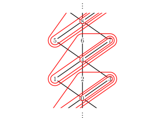
$\tilde{P}$ A maximal tubing of $\tilde{P}$

Figure 2. An affine poset of order $4$ and a maximal tubing

Definition 2.6.

For an affine poset $\tilde{P}$, the affine poset cyclohedron $\mathscr{C}(\tilde{P})$ is a simple, convex polytope of dimension $|\tilde{P}|-1$ whose face lattice is isomorphic to the set of proper tubings ordered by reverse inclusion. Vertices of $\mathscr{C}(\tilde{P})$ correspond to maximal tubings of $\tilde{P}$.

We also realize affine poset cyclohedra as an intersection of half-spaces. Let $\tilde{P}$ be an affine poset and let $n=|\tilde{P}|$. Fix some constant $c\in\mathbb{R}^{+}$. We define the space of affine maps $\mathbb{R}^{\tilde{P}}$ as the set of bi-infinite sequences $\mathbf{\tilde{x}}=(\tilde{x}_{i})_{i\in\mathbb{Z}}$ such that $\tilde{x}_{i}=\tilde{x}_{i+n}+c$ for all $i\in\mathbb{Z}$. Let $\mathcal{C}\subset\mathbb{R}^{\tilde{P}}$ be the subspace consisting of all constant maps. We work in the ambient space $\mathbb{R}^{\tilde{P}}/\mathcal{C}$ where the constant $c$ in the definition of affine maps is given by $c=n^{2(n+1)}$.

For a finite subset $\tau\subseteq P$, define a linear function $\alpha_{\tau}$ on $\mathbb{R}^{\tilde{P}}/\mathcal{C}$ by

$$\alpha_{\tau}(\mathbf{\tilde{x}}):=\sum\limits_{\begin{subarray}{c}i\prec\mathrel{\mkern-5.0mu}\mathrel{\cdot}j\\ i,j\in\tau\end{subarray}}\tilde{x}_{j}-\tilde{x}_{i}.$$

Again, the sum is taken over all covering relations contained in $\tau$. We define the half-space $h_{\tau}$ and the hyperplane $H_{\tau}$ by

$$h_{\tau} :=\{p\in\mathbb{R}^{\tilde{P}}/{\mathcal{C}}\mid\alpha_{\tau}(p)\geq n^{2|\tau|}\}$$ and

$$H_{\tau} :=\{p\in\mathbb{R}^{\tilde{P}}/{\mathcal{C}}\mid\alpha_{\tau}(p)=n^{2|\tau|}\}.$$

Remark 2.7.

Observe that for any tube $\tau$ and $k\in\mathbb{Z}$, $h_{\tau}=h_{\tau+kn}$.

The following is our main result in the affine case:

Theorem 2.8.

If $\tilde{P}$ is an affine poset, the intersection of $h_{\tau}$ for all proper tubes $\tau$ gives a realization of $\mathscr{C}(\tilde{P})$.

2.3. An interpretation of tubings

When $P$ is a chain, $\mathscr{A}(P)$ recovers the classical associahedron. There is a simple interpretation of proper tubings that explains all of the conditions above in terms of generalized words.

We can understand the classical associahedron as follows: Let $P=(\{1,...,n\},\leq)$ be a chain. We can think of the chain as a word we want to multiply together with the rule that two elements can be multiplied if they are connected by an edge. A maximal tubing of $P$ is a way of disambiguating the order in which one performs the multiplication. If a pair of adjacent elements $x$ and $y$ have a pair of brackets around them, they contract along the edge connecting them and replace $x$ and $y$ by their product.

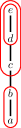
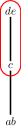
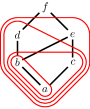
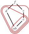
Figure 3. Multiplication of a word and of a generalized word

Similarly, we can understand the Hasse diagram of an arbitrary poset $P$ as a generalized word we would like to multiply together. Again, we are allowed to multiply two elements if they are connected by an edge, but when multiplying elements, we contract along the edge connecting them and then take the transitive reduction of the resulting directed graph. That is, we identify the two elements and take the resulting quotient poset. A maximal tubing is again a way of disambiguating the order of the multiplication. See Figure 3 for an illustration of this multiplication. This perspective is discussed in relation to operahedra in [9, Section 2.1] when the Hasse diagram of $P$ is a rooted tree.

3. Configuration spaces and compactifications

We turn our attention to the relationship between poset associahedra and configuration spaces. For a poset $P$, the order cone

$$\mathscr{L}(P):=\{p\in\mathbb{R}^{P}_{\Sigma=0}\mid p_{i}\leq p_{j}\text{ for all }i\preceq j\}$$

is the set of order preserving maps $P\to\mathbb{R}$ whose values sum to $0$.

Fix a constant $c\in\mathbb{R}^{+}$. The order polytope, first defined by Stanley [14] and extended by Galashin [6], is the $(|P|-2)$-dimensional polytope

$$\mathscr{O}(P):=\{p\in\mathscr{L}(P)\mid\alpha_{P}(p)=c\}.$$

Remark 3.1.

When $P$ is bounded, that is, has a unique maximum $\hat{1}$ and minimum $\hat{0}$, this construction is projectively equivalent to Stanley’s order polytope where we replace the conditions of the coordinates summing to $0$ and $\alpha_{P}(p)=c$ with the conditions $p_{\hat{0}}=0$ and $p_{\hat{1}}=1$, see [6, Remark 2.5].

Galashin [6] obtains the poset associahedra by an alternative compactification of $\mathscr{O}^{\circ}(P)$, the interior of $\mathscr{O}(P)$. We describe this compactification informally, as it serves as motivation for the realization in Theorem 2.3.

A point is on the boundary of $\mathscr{O}(P)$ when any of the inequalities in the order cone achieve equality. The faces of of $\mathscr{O}(P)$ are in bijection with proper tubings of $P$ such that all tubes are disjoint. Let $T$ be such a tubing. If $p$ is in the face corresponding to $T$ and $\tau\in T$ then $p_{i}=p_{j}$ for $i,j\in\tau$.

We can think of the point $p$ in the face corresponding to $T$ as being “what happens in $\mathscr{O}(P)$” when for each $\tau\in T$, the coordinates are infinitesimally close. However, by taking all coordinates in $\tau$ to be equal, we lose information about their relative ordering. In $\mathscr{A}(P)$, we still think of the coordinates in $\tau$ as being infinitesimally close, but we are still interested in their configuration. Upon zooming in, this is parameterized by the order polytope of the subposet $(\tau,\preceq)$. We iterate this process, allowing points in $\tau$ to be infinitesimally closer, and so on. We illustrate this in Figure 4. This idea is a common explanation of the Axelrod–Singer compactification of $\mathscr{O}^{\circ}(P)$ when $P$ is a chain, see [1, 8, 13].

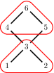
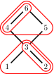
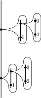
Tubing in $\mathscr{O}(P)$ Point in $\mathscr{O}(P)$ Tubing in $\mathscr{A}(P)$ Point in $\mathscr{A}(P)$

Figure 4. A vertex in $\mathscr{O}(P)$ vs. $\mathscr{A}(P).$

The idea of the realization in Theorem 2.3 is to replace the notions of infinitesimally close and infinitesimally closer with being exponentially close and exponentially closer. For $p\in\mathscr{L}(P)$, $\alpha_{\tau}$ acts a measure of how close the coordinates of $p|_{\tau}$ are. We can make this precise with the following definition and lemma.

Definition 3.2.

For $S\subseteq P$ and $p\in\mathbb{R}^{P}$, define the diameter of $p$ relative to $S$ by

$$\operatorname{diam}_{S}(p)=\max\limits_{i,j\in S}|p_{i}-p_{j}|.$$

That is, $\operatorname{diam}_{S}(p)$ is the diameter of $\{p_{i}:i\in S\}$ as a subset of $\mathbb{R}$.

Lemma 3.3.

Let $\tau\subseteq P$ be a tube and let $p\in\mathscr{L}(P)$. Then

$$\operatorname{diam}_{\tau}(p)\leq\alpha_{\tau}(p)\leq\frac{n^{2}}{4}\operatorname{diam}_{\tau}(p).$$

Proof.

By the triangle inequality and as $\tau$ is connected, $\operatorname{diam}_{\tau}(p)\leq\alpha_{\tau}(p)$. For the other inequality,

$$\alpha_{\tau}(p) =\sum\limits_{\begin{subarray}{c}i\prec\mathrel{\mkern-5.0mu}\mathrel{\cdot}j\\ i,j\in\tau\end{subarray}}p_{j}-p_{i}$$

$$\leq\sum\limits_{\begin{subarray}{c}i\prec\mathrel{\mkern-5.0mu}\mathrel{\cdot}j\\ i,j\in\tau\end{subarray}}\operatorname{diam}_{\tau}(p)$$

$$\leq\frac{1}{4}n^{2}\operatorname{diam}_{\tau}(p)$$

The inequality in the last line comes from the fact that there are at most $\frac{n^{2}}{4}$ covering relations in $P$, which follows from Mantel’s Theorem and the fact that Hasse diagrams are triangle-free.

∎

In particular, for $p\in\mathscr{L}(P)$, if $p\in H_{\tau}$, then $\{p_{i}\mid i\in\tau\}$ is clustered tightly together compared to any tube containing $\tau$. If $p\in h_{\tau}$, then $\{p_{i}\mid i\in\tau\}$ is spread far apart compared to any tube contained in $\tau$.

4. Realizing poset associahedra

We are now prepared to prove Theorem 2.3. Define

$$\mathscr{A}(P):=\bigcap\limits_{\sigma\subset P}h_{\sigma}\cap H_{P}$$

where the intersection is over all tubes of $P$. Note that $\mathscr{A}(P)\subseteq\mathscr{L}(P)$ as if $i\prec\mathrel{\mkern-5.0mu}\mathrel{\cdot}j$ is a covering relation, then for $p\in h_{\{i,j\}}$, $p_{i}\leq p_{j}$.

Theorem 2.3 follows as a result of three lemmas:

Lemma 4.1.

If $T$ is a maximal tubing, then

$$v^{T}:=\bigcap\limits_{\tau\in T\cup\{P\}}H_{\tau}$$

is a point.

Lemma 4.2.

If $T$ is a collection of tubes that do not form a proper tubing, then

$$\bigcap\limits_{\tau\in T}H_{\tau}\cap\mathscr{A}(P)=\emptyset.$$

Lemma 4.3.

If $T$ is a maximal tubing and $\tau\notin T$ is a proper tube, then $\alpha_{\tau}(v^{T})>n^{2|\tau|}.$ That is, $v^{T}$ lies in the interior of $h_{\tau}$.

Lemma 4.1 follows from a standard induction argument.

Proof of Lemma 4.2.

If $T$ is not a collection of tubes that do proper tubing, then at least one of the following two cases holds:

1. There is a pair of non-nested and non-disjoint tubes $\tau_{1},\tau_{2}$ in $T$.

2. There is a sequence of disjoint tubes $\tau_{1},...,\tau_{k}$ such that $\tau_{1}\prec\dots\prec\tau_{k}\prec\tau_{1}$.

The idea of the proof is as follows: For $S\subseteq P$, define the convex hull of $S$ as

$$\operatorname{conv}(\sigma):=\{b\in P\mid\exists a,c\in S:a\leq b\leq c\}.$$

Observe that if $p\in\mathscr{L}(P),$ then $\operatorname{diam}_{S}(p)\leq\operatorname{diam}_{\operatorname{conv}(S)}(p)$. Take $\sigma=\operatorname{conv}(\tau_{1}\cup\dots\cup\tau_{k})$. One can show that $\sigma$ is a tube, so Lemma 3.3 tells us that for each $\tau_{i}$, $\operatorname{diam}_{\tau_{i}}(p)$ is very small compared to $n^{2|\sigma|}$. As the tubes either intersect or are cyclic, one can show this forces $\operatorname{diam}_{\sigma}(p)$ to also be small, so $\alpha_{\sigma}(p)<n^{2|\sigma|}$.

More concretely, suppose that

$$p\in\bigcap H_{\tau_{i}}\cap\mathscr{L}(P).$$

Note that for all $i$, $|\sigma|>|\tau_{i}|+1$ and $\operatorname{diam}_{\tau_{i}}(p)\leq n^{2(|\sigma|-1)}$. In case (1), let $a,b\in\sigma$. There exists some $x\in\tau_{1}\cap\tau_{2}$, so

$$|p_{a}-p_{b}| \leq|p_{a}-p_{x}|+|p_{x}-p_{b}|$$

$$\leq\operatorname{diam}_{\tau_{1}}(p)+\operatorname{diam}_{\tau_{2}}(p)$$

$$\leq 2n^{2(|\sigma|-1)}$$

$$<n^{2(|\sigma|)}.$$

Hence $\operatorname{diam}_{\sigma}(p)<n^{2|\sigma|}$, so by Lemma 3.3, $p\notin h_{\sigma}$.

Now we move to case (2). Suppose there is a sequence of disjoint tubes $\tau_{1},...,\tau_{k}$ such that for each $i$ there exists $x_{i},y_{i}\in\tau_{i}$ where $x_{i}\prec y_{i+1}$ where we take the indices $\text{mod }{k}$. Then:

$$p_{y_{i}}-\operatorname{diam}_{\tau_{i}}(p) \leq p_{x_{i}}$$

$$p_{x_{i}} \leq p_{y_{i+1}}$$

$$p_{y_{i+1}} \leq p_{x_{i+1}}+\operatorname{diam}_{\tau_{i+1}}$$

Furthermore, since $\tau_{i}\text{ and }\tau_{i+1}$ are disjoint, $|\tau_{i}|\leq|\sigma|-2$ and $\operatorname{diam}_{\tau_{i}}\leq n^{2(|\sigma|-2)}$. Combining these we get

$$p_{y_{i}}\leq p_{y_{i+1}}+2n^{2(|\sigma|-2)}.$$

Then we have:

$$p_{y_{1}} \leq p_{y_{i}}+2in^{2(|\sigma|-2)}$$ and

$$p_{y_{i}}+2in^{2(|\sigma|-2)} \leq p_{y_{1}}+2(k+1)n^{2(|\sigma|-2)}.$$

These yield

$$p_{y_{1}}-p_{y_{i}} \leq 2in^{2(|\sigma|-2)}$$ and

$$p_{y_{i}}-p_{y_{1}} \leq 2(k-i+1)n^{2(|\sigma|-2)}.$$

As $i,k-i+1\leq k\leq\frac{n}{2}$, we have $|p_{y_{1}}-p_{y_{i}}|\leq n^{2(|\sigma|-1)}$. Finally, if $z_{i}\in\tau_{i},z_{j}\in\tau_{j}$, then

$$|p_{z_{i}}-p_{z_{j}}| \leq|p_{z_{i}}-p_{y_{i}}|+|p_{y_{i}}-p_{y_{1}}|+|p_{y_{1}}-p_{y_{j}}|+|p_{y_{j}}-p_{z_{j}}|$$

$$\leq 4n^{2(|\sigma|-1)}$$

$$<n^{2|\sigma|}.$$

Hence $\operatorname{diam}_{\sigma}(p)<n^{2|\sigma|}$, and by Lemma 3.3, $p\notin h_{\sigma}$.

∎

Proof of Lemma 4.3.

Let $T$ be a maximal tubing of $P$ and let $\tau\notin T$ be a tube. Define the convex hull of $\tau$ relative to $T$ by

$$\operatorname{conv}_{T}(\tau):=\min\{\sigma\in T\mid\tau\subset\sigma\}.$$

Let $\sigma=\operatorname{conv}_{T}(\tau)$. $T$ partitions $\sigma$ into a lower set $A$ and an upper set $B$ where $A$ and $B$ are either tubes or singletons. Furthermore, $A$ and $B$ both intersect $\tau$. See Figure 5 for an example illustrating this.

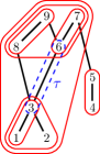
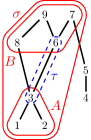
Maximal Tubing $T$ and tube $\tau$ $\sigma,A,$ and $B$ labelled

Figure 5. An example illustrating the proof of Lemma 4.3.

The idea of the proof is as follows: Let $p=v^{T}$. By Lemma 3.3, $\operatorname{diam}_{A}(p)$ and $\operatorname{diam}_{B}(p)$ are both very small compared to $\operatorname{diam}_{\sigma}(p)$. Then for any $a\in A,b\in B$, $|p_{a}-p_{b}|$ must be large. As $\tau$ intersects both $A$ and $B$, $\operatorname{diam}_{\tau}(p)$ must be large and hence $p\in h_{\tau}$. See Figure 6 for an illustration of this. More precisely, we show that for any $i\in A,j\in B$, $p_{j}-p_{i}>(n^{2})^{|\tau|}$, which implies that $p$ lies in the interior of $h_{\tau}$.

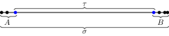
Figure 6. If $\operatorname{diam}_{A}(p)$ and $\operatorname{diam}_{B}(p)$ are small and $\operatorname{diam}_{\sigma}(p)$ is large, then $\operatorname{diam}_{\tau}(p)$ is large.

Observe that:

$$\sum\limits_{x\prec\mathrel{\mkern-5.0mu}\mathrel{\cdot}y}p_{y}-p_{x}=\underbrace{\sum\limits_{\begin{subarray}{c}x\prec\mathrel{\mkern-5.0mu}\mathrel{\cdot}y\\ x,y\in A\end{subarray}}(p_{y}-p_{x})}_{\begin{subarray}{c}\leq(n^{2})^{|\sigma|-1}\\ <\frac{1}{8}(n^{2})^{|\sigma|}\end{subarray}}+\underbrace{\sum\limits_{\begin{subarray}{c}x\prec\mathrel{\mkern-5.0mu}\mathrel{\cdot}y\\ x,y\in B\end{subarray}}(p_{y}-p_{x})}_{\begin{subarray}{c}\leq(n^{2})^{|\sigma|-1}\\ <\frac{1}{8}(n^{2})^{|\sigma|}\end{subarray}}+\sum\limits_{\begin{subarray}{c}x\prec\mathrel{\mkern-5.0mu}\mathrel{\cdot}y\\ x\in A,y\in B\end{subarray}}(p_{y}-p_{x}).$$

Fix $i\in A\text{ and }j\in B$. By Lemma 3.3, for any $x\in A,y\in B$,

$$p_{y}-p_{x} \leq p_{j}-p_{i}+\operatorname{diam}_{A}(p)+\operatorname{diam}_{B}(p)$$

$$\leq p_{j}+p_{i}+2n^{2(|\sigma|-1)}.$$

Again, noting that the number of covering relations in $\sigma$ is at most $\frac{n^{2}}{4}$ we obtain:

$$\sum\limits_{\begin{subarray}{c}x\prec\mathrel{\mkern-5.0mu}\mathrel{\cdot}_{\sigma}y\\ x\in A,y\in B\end{subarray}}(p_{y}-p_{x}) \leq\sum\limits_{\begin{subarray}{c}x\prec\mathrel{\mkern-5.0mu}\mathrel{\cdot}_{\sigma}y\\ x\in A,y\in B\end{subarray}}(p_{j}-p_{i}+2(n^{2})^{|\sigma|-1})$$

$$\leq\frac{n^{2}}{4}\left(p_{j}-p_{i}+2(n^{2})^{|\sigma|-1}\right)$$

$$=\frac{n^{2}}{4}(p_{j}-p_{i})+\frac{1}{2}(n^{2})^{|\sigma|}.$$

Combining all of this we get:

$$\sum\limits_{x\prec\mathrel{\mkern-5.0mu}\mathrel{\cdot}_{\sigma}y}p_{y}-p_{x} =(n^{2})^{|\sigma|}$$

$$<\frac{1}{8}(n^{2})^{|\sigma|}+\frac{1}{8}(n^{2})^{|\sigma|}+\frac{1}{2}(n^{2})^{|\sigma|}+\frac{n^{2}}{4}(p_{j}-p_{i})$$

$$\leq\frac{3}{4}(n^{2})^{|\sigma|}+\frac{n^{2}}{4}(p_{j}-p_{i})$$

Then $(n^{2})^{|\sigma|-1}<(p_{j}-p_{i})$ and as $|\tau|\leq|\sigma|-1$, $p$ is in the interior of $h_{\tau}$.

∎

Remark 4.4.

A similar approach for realizing graph associahedra is taken by Devadoss [4]. For a graph $G=(V,E)$, Devadoss realizes the graph associahedron of $G$ by taking the supporting hyperplane for a graph tube $\tau$ to be

$$\left\{p\in\mathbb{R}^{V}\mid\sum\limits_{i\in\tau}p_{i}=3^{|\tau|}\right\}.$$

One difference is that Devadoss realizes graph associahedra by cutting off slices of a simplex whereas we cut off slices of an order polytope. When the Hasse diagram of $P$ is a tree, the poset associahedron is combinatorially equivalent to the graph associahedron of the line graph of the Hasse diagram. In this case, the two realizations have linearly equivalent normal fans. If the Hasse diagram of $P$ is a path graph, then both realizations have linearly equivalent normal fans to the realization of the associahedron due to Shnider and Sternberg [15].

5. Realizing affine poset cyclohedra

The proofs in the affine case are nearly identical to the finite case with some additional technical components. The similarity comes from the fact that Lemma 3.3 still applies. We highlight where the proofs are different. Let $\tilde{P}$ be an affine poset of order $n$.

Define

$$\mathscr{C}(\tilde{P}) :=\bigcap\limits_{\sigma\subset P}h_{\sigma}$$ and

$$\mathscr{L}(\tilde{P}) :=\{p\in\mathbb{R}^{\tilde{P}}/\mathcal{C}\mid p_{i}\leq p_{j}\text{ for all }i\preceq j\}.$$

where the intersection is over all tubes of $\tilde{P}$. Note that $\mathscr{C}(\tilde{P})\subseteq\mathscr{L}(\tilde{P})$ as if $i\prec\mathrel{\mkern-5.0mu}\mathrel{\cdot}j$ is a covering relation, then for $p\in h_{\{i,j\}}$, $p_{i}\leq p_{j}$. Theorem 2.8 follows as a result of 3 lemmas:

Lemma 5.1.

If $T$ is a maximal tubing, then

$$v^{T}:=\bigcap\limits_{\tau\in T}H_{\tau}$$

is a point.

Lemma 5.2.

If $T$ is a collection of tubes that do not form a proper tubing, then

$$\bigcap\limits_{\tau\in T}H_{\tau}\cap\mathscr{C}(\tilde{P})=\emptyset.$$

Lemma 5.3.

If $T$ is a maximal tubing and $\tau\notin T$ is a proper tube, then $\alpha_{\tau}(v^{T})>n^{2|\tau|}.$ That is, $v^{T}$ lies in the interior of $h_{\tau}$.

Proof of Lemma 5.1.

Let $T$ be a maximal tubing and take any $\sigma\in T$ such that $|\tau|=n$. Then restricting to $\tilde{P}|_{\sigma}$, Lemma 4.1 implies that

$$\bigcap\limits_{\begin{subarray}{c}\tau\in T\\ \tau\subseteq\sigma\end{subarray}}H_{\tau}$$

is a point. However, as $T$ is $n$-periodic,

$$\bigcap\limits_{\begin{subarray}{c}\tau\in T\\ \tau\subseteq\sigma\end{subarray}}H_{\tau}=\bigcap\limits_{\begin{subarray}{c}\tau\in T\end{subarray}}H_{\tau}.$$

∎

Proof of Lemma 5.2.

By Remark 2.7, we can assume $T$ is $n$-periodic. The proof is almost identical to the proof of Lemma 4.2. Define

$$\mathscr{L}(\tilde{P}):=\{p\in\mathbb{R}^{\tilde{P}}/\mathcal{C}\mid p_{i}\leq p_{j}\text{ for all }i\preceq j\}.$$

and note that

$$\mathscr{L}(\tilde{P})\subseteq R^{\tilde{P}}/\mathcal{C}\bigcap\limits_{\begin{subarray}{c}i,j\in\tilde{P}\\ i\prec\mathrel{\mkern-5.0mu}\mathrel{\cdot}j\end{subarray}}h_{\{i,j\}}.$$

Let

$$p\in\bigcap H_{\tau_{i}}\cap\mathscr{L}(\tilde{P}).$$

We again break into two cases:

1. There is a pair of non-nested and non-disjoint tubes $\tau_{1},\tau_{2}$ in $T$.

2. All tubes in $T$ are pairwise nested or disjoint and there is a sequence of disjoint tubes $\tau_{1},...,\tau_{k}$ such that $\tau_{1}\prec\dots\prec\tau_{k}\prec\tau_{1}$.

The only difference in the proof occurs in case (1). Here, it is possible that there exists $x\in\tau_{1}\cup\tau_{2}$ such that $x+n\in\tau_{1}\cup\tau_{2}$ as well. In this case, the proof of Lemma 4.2 still implies that $\operatorname{diam}_{\tau_{1}\cup\tau_{2}}(p)\leq\operatorname{diam}_{\tau_{1}}(p)+\operatorname{diam}_{\tau_{2}}(p)\leq 2n^{2n}$. However, $|p_{x+n}-p_{x}|=n^{2(n+1)}$.

∎

Proof of Lemma 5.3.

Let $T$ be a maximal tubing and $\tau\notin T$ be a proper tube. Let $p=v^{T}$. We claim that $\alpha_{\tau}(p)>n^{2|\tau|}.$

The only difference from the proof of Lemma 4.3 is that $\tau$ may not be contained by any tube in $\tau$ so $\operatorname{conv}_{T}(\tau)$ may not be well-defined. In this case, there exists $A\in T$ such that $|A|=n$, $A\cap\tau\neq\emptyset,\text{ and }(A+n)\cap\tau\neq\emptyset$. Here, $(A+n)$ acts the same as $B$ in the finite case, except the argument is much simpler.

Let $i\in A\cap\tau,j\in(A+n)\cap\tau$. Observe that $\operatorname{diam}_{A}(p),\operatorname{diam}_{(A+n)}(p)\leq n^{2n}$ and that $i+n\in(A+n)$. Then

$$|p_{j}-p_{i}| \geq(p_{j}-n^{2n})-p_{i}$$

$$\geq p_{i+n}-p_{i}$$

$$=n^{2(n+1)}.$$

Hence $\operatorname{diam}_{\tau}(p)>n^{2|\tau|}$ and by Lemma 3.3, $\alpha_{\tau}(p)>n^{2|\tau|}$.

∎

6. Remarks and Questions

Remark 6.1.

Let $(P,\preceq)$ be a bounded poset. In Remark 3.1, we discuss how $\mathscr{O}(P)$ can be realized as the set of all $p\in\mathbb{R}^{P}$ such that $p_{\hat{0}}=0$, $p_{\hat{1}}=1$, and $p_{i}\leq p_{j}$ whenever $i\preceq j$. We can similarly realize $\mathscr{A}(P)$ as follows: Fix $0<\varepsilon<\frac{1}{n^{2}}$.

For a proper tube $\tau\subset P$, let

$$h^{\prime}_{\tau}=\{p\in\mathbb{R}^{P}\mid\alpha_{\tau}(p)<\varepsilon^{n-|\tau|}\}.$$

Then $\mathscr{A}(P)$ is realized as the intersection over all $h^{\prime}_{\tau}$ with the hyperplanes

$$\{p_{\hat{0}}=0\}\text{ and }\{p_{\hat{1}}=1\}.$$

Letting $\varepsilon\to 0$, we obtain $\mathscr{O}(P)$ as a limit of $\mathscr{A}(P)$ as shown in Figure 7.

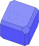
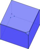
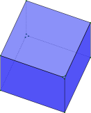
$P$ $\varepsilon=\frac{1}{3}$ $\varepsilon=\frac{1}{9}$ $\varepsilon=\frac{1}{27}$

Figure 7. $\mathscr{O}(P)$ as a limit of $\mathscr{A}(P)$

Remark 6.2.

The key piece to the realizations in Theorems 2.3 and 2.8 is the linear form $\alpha_{\tau}$, where $\alpha_{\tau}$ acts as an approximation of $\operatorname{diam}_{\tau}$. In particular, let $\tau$ be a tube and let $p\in\mathscr{L}(P)$. Then:

• $\alpha_{\tau}(p)\geq 0$.

• $\alpha_{\tau}(p)=0\Leftrightarrow p|_{\tau}$ is constant.

• If $\sigma\subseteq\tau$ is a tube, then $\alpha_{\sigma}(p)\leq\alpha_{\tau}(p)$.

However, there are many other options for choice of $\alpha_{\tau}$ that could fill this role. Some other options include:

1. Sum over all pairs $i\prec j$ in $\tau$.

   $$\alpha_{\tau}(p)=\sum\limits_{\begin{subarray}{c}i\prec j\\ i,j\in\tau\end{subarray}}p_{j}-p_{i}.$$

2. Let $A\text{ and }B$ be the set of minima and maxima of the restriction $P|_{\tau}$ respectively.

   $$\alpha_{\tau}(p)=\sum\limits_{\begin{subarray}{c}i\prec j\\ i\in A,j\in B\end{subarray}}p_{j}-p_{i}.$$

3. Fix a spanning tree $T$ in the Hasse diagram of $\tau$. Let $E=\{(i,j)\mid i\prec\mathrel{\mkern-5.0mu}\mathrel{\cdot}_{T}j\}$ be the set of edges in $T$.

   $$\alpha_{\tau}(p)=\sum\limits_{(i,j)\in E}p_{j}-p_{i}.$$

   An advantage of this option is that we would have

   $$\operatorname{diam}_{\tau}(p)\leq\alpha_{\tau}(p)\leq(n-1)\operatorname{diam}_{\tau}(p).$$

A similar realization can be obtained for each choice of of $\alpha_{\tau}$.

Question 6.3.

Recall that for a simple $d$-dimensional polytope $P$, the $f$-vector and $h$-vector of $P$ are given by $(f_{0},\dots,f_{d})$ and $(h_{0},\dots,h_{d})$ where $f_{i}$ is the number of $i$-dimensional faces and

$$\sum\limits_{i=0}^{d}f_{i}t^{i}=\sum\limits_{i=0}^{d}h_{i}(t+1)^{i}.$$

Postnikov, Reiner, and Williams [12] found a statistic on maximal tubings of graph associahedra of chordal graphs where

$$\sum\limits_{T}t^{\operatorname{stat}(T)}=\sum h_{i}t^{i}.$$

In particular, they define a map $T\mapsto w_{T}$ from maximal tubings of a graph on $n$ vertices to the set of permutations $S_{n}$ such that $\operatorname{stat}(T)=\operatorname{des}(w_{T})$, the number of descents of $w_{T}$. It would be interesting to find a similar statistic on maximal tubings of poset associahedra. For a simple polytope $P$, one can orient the edges of $P$ according to a generic linear form and take $\operatorname{stat}(v)=\operatorname{outdegree}(v)$ [17, §8.2]. It may be possible to use our realization to find the desired statistic.

References

- [1] Scott Axelrod and Isadore M Singer “Chern-Simons perturbation theory. II” In Journal of Differential Geometry 39.1 Lehigh University, 1994, pp. 173–213
- [2] Raoul Bott and Clifford Taubes “On the self-linking of knots” In Journal of Mathematical Physics 35.10 American Institute of Physics, 1994, pp. 5247–5287
- [3] Michael Carr and Satyan L Devadoss “Coxeter complexes and graph-associahedra” In Topology and its Applications 153.12 Elsevier, 2006, pp. 2155–2168
- [4] Satyan L Devadoss “A realization of graph associahedra” In Discrete Mathematics 309.1 Elsevier, 2009, pp. 271–276
- [5] Sergey Fomin and Nathan Reading “Root systems and generalized associahedra” In arXiv preprint math/0505518, 2005
- [6] Pavel Galashin “Poset associahedra” In arXiv preprint arXiv:2110.07257, 2021
- [7] Mark Haiman “Constructing the associahedron” In Unpublished manuscript, MIT, 1984
- [8] Pascal Lambrechts, Victor Turchin and Ismar Volić “Associahedron, cyclohedron and permutohedron as compactifications of configuration spaces” In Bulletin of the Belgian Mathematical Society-Simon Stevin 17.2 The Belgian Mathematical Society, 2010, pp. 303–332
- [9] Guillaume Laplante-Anfossi “The diagonal of the operahedra” In Advances in Mathematics 405 Elsevier, 2022, pp. 108494
- [10] Chiara Mantovani, Arnau Padrol and Vincent Pilaud “Acyclonestohedra: when oriented matroids meet nestohedra”, in prep.
- [11] Kyle Petersen “Eulerian Numbers”, 2015 DOI: 10.1007/978-1-4939-3091-3
- [12] Alex Postnikov, Victor Reiner and Lauren Williams “Faces of Generalized Permutohedra” In Documenta Mathematica 13, 2008, pp. 207–273
- [13] Dev P Sinha “Manifold-theoretic compactifications of configuration spaces” In Selecta Mathematica 10.3 Springer, 2004, pp. 391–428
- [14] Richard P Stanley “Two poset polytopes” In Discrete & Computational Geometry 1.1 Springer, 1986, pp. 9–23
- [15] Jim Stasheff “From Operads to ‘Physically’ Inspired Theories”, 1996
- [16] Dov Tamari “Monoïdes préordonnés et chaînes de Malcev” In Bulletin de la Société mathématique de France 82, 1954, pp. 53–96
- [17] Günter M Ziegler “Lectures on polytopes” Springer Science & Business Media, 2012