The $S$-diagnostic—an a posteriori error assessment for single-reference coupled-cluster methods

Abstract

We propose a novel a posteriori error assessment for the single-reference coupled-cluster (SRCC) method called the $S$-diagnostic. We provide a derivation of the $S$-diagnostic that is rooted in the mathematical analysis of different SRCC variants. We numerically scrutinized the $S$-diagnostic, testing its performance for (1) geometry optimizations, (2) electronic correlation simulations of systems with varying numerical difficulty, and (3) the square-planar copper complexes [CuCl₄]^2-, [Cu(NH₃)₄]²⁺, and [Cu(H₂O)₄]²⁺. Throughout the numerical investigations, the $S$-diagnostic is compared to other SRCC diagnostic procedures, that is, the $T_{1}$, $D_{1}$, and $D_{2}$ diagnostics as well as different indices of multi-determinantal and multi-reference character in coupled-cluster theory. Our numerical investigations show that the $S$-diagnostic outperforms the $T_{1}$, $D_{1}$, and $D_{2}$ diagnostics and is comparable to the indices of multi-determinantal and multi-reference character in coupled-cluster theory in their individual fields of applicability. The experiments investigating the performance of the $S$-diagnostic for geometry optimizations using SRCC reveal that the $S$-diagnostic correlates well with different error measures at a high level of statistical relevance. The experiments investigating the performance of the $S$-diagnostic for electronic correlation simulations show that the $S$-diagnostic correctly predicts strong multi-reference regimes. The $S$-diagnostic moreover correctly detects the successful SRCC computations for [CuCl₄]^2-, [Cu(NH₃)₄]²⁺, and [Cu(H₂O)₄]²⁺, which have been known to be misdiagnosed by $T_{1}$ and $D_{1}$ diagnostics in the past. This shows that the $S$-diagnostic is a promising candidate for an a posteriori diagnostic for SRCC calculations.

[Second University] Hylleraas Centre for Quantum Molecular Sciences, Department of Chemistry, University of Oslo, Norway IR,NMR,UV

1 Introduction

While the underlying mathematical theory of the quantum many-body problem is, on a fundamental level, well described, the governing equation, namely, the many-body Schrödinger equation, remains numerically intractable for a large number of particles. In fact, the many-body Schrödinger equation poses one of today’s hardest numerical challenges, mainly due to the exponential growth in computational complexity with the number of electrons. Over the past century, numerous numerical approximation techniques of various levels of cost and accuracy have been developed in order to overcome this curse of dimensionality. Arguably, the most successful approaches are based on coupled-cluster (CC) theory ¹, which defines a cost-efficient hierarchy of increasingly accurate methods, including the so-called gold standard of quantum chemistry—the coupled-cluster singles-and-doubles with perturbative triples (CCSD(T)) ² model.

Despite the great success of CC theory, its reliability is not yet fully quantifiable. More precisely, aside from a few heuristically derived results, there exists no universally reliable diagnostic that indicates if the computational result is to be trusted. This shortcoming is most apparent in the regime of transition metal compounds and molecular bond breaking/making processes, systems dominated by strong nondynamic electron-correlation effects, where several methods based on CC theory tend to fail along with all other numerically tractable approaches.

Therefore, a posteriori error diagnostics are urgently needed in the field. Until very recently, the diagnostic approaches available were limited to the so-called $T_{1}$ (also called $\tau_{1}$) ^{3, 4}, $D_{1}$, and $D_{2}$ diagnostic ^{5, 6}. Despite clear numerical evidence that diagnostics based on the single excitation amplitudes, such as the $T_{1}$ and $D_{1}$ diagnostics, do not provide reliable indicators ⁷, they are commonly used due to the lack of alternatives. Recently, an alternative set of multi-reference indices was introduced which provided a number of a posteriori diagnostic tools ⁸ christened the indices of multi-determinantal and multi-reference character in coupled-cluster theory. These tools are highly descriptive and able to determine different molecular scenarios in which CC theory may fail.

We provide an alternative error diagnostic that is based on assumptions employed in the mathematical analysis CC theory. More precisely, our diagnostic is derived from the mathematical analysis of CC theory that provides sufficient conditions for a locally unique and quasi-optimal solution to the CC working equations. Central to our derivation is the strong monotonicity property, as introduced by Schneider ⁹, which is eponymous for our S-diagnostic. Compared to the recently suggested nine indices that describe the multi-determinantal and multi-reference character in coupled-cluster theory ⁸, the $S$-diagnostic is a diagnostic technique that can be applied to multi-determinantal and multi-reference scenarios alike. We complement our theoretical derivation of the $S$-diagnostic with numerical simulations scrutinizing its validity for different geometry optimizations, and electronic correlation computations for systems of varying numerical difficulty for single reference coupled-cluster methods.

The rest of the article is structured as follows. We begin with a brief review of CC theory, followed by a short summary of the mathematical results derived in previous works which lay the mathematical foundation for the proposed $S$-diagnostics. Then, we derive the main result, i.e., the $S$-diagnostic which is subsequently numerically scrutinized.

2 Theory

2.1 Brief overview of coupled-cluster theory

In CC theory the wave function is parametrized by the exponential $|\psi\rangle=e^{\hat{T}}|\phi_{0}\rangle$. Here, $|\phi_{0}\rangle$ is the reference determinant defining the occupied spin orbitals, and $\hat{T}=\sum_{\mu}t_{\mu}\hat{X}_{\mu}=\sum_{k}\hat{T}_{k}$ is a cluster operator, where $\hat{T}_{k}$ excites $k=1,\dots,N$ electrons—$k$ is the excitation rank of a given $\hat{T}_{k}$—from the occupied spin orbitals into the virtual spin-orbitals. All possible excited determinants can be expressed as $|\mu\rangle=\hat{X}_{\mu}|\phi_{0}\rangle$ for some multi-index $\mu$ labeling occupied and virtual spin-orbitals. The governing equations determining amplitudes $(t_{\mu})$, and therewith also the CC energy $\mathcal{E}_{\rm CC}(t)$, are given by $f_{\mathrm{CC}}(t)=0$, where

$$\left\{\begin{aligned} \mathcal{E}_{\rm CC}(t)&=\langle\phi_{0}|e^{-\hat{T}}\hat{H}e^{\hat{T}}|\phi_{0}\rangle\\ (f_{\mathrm{CC}}(t))_{\mu}&=\langle\mu|e^{-\hat{T}}\hat{H}e^{\hat{T}}|\phi_{0}\rangle.\end{aligned}\right.$$ (1)

More compactly, Eq. 1 can be expressed using the CC Lagrangian ^{10, 11}

$$\mathcal{L}(t,z)=\mathcal{E}_{\mathrm{CC}}(t)+\sum_{\mu}z_{\mu}(f_{\mathrm{CC}}(t))_{\mu}=\langle\phi_{0}|(\hat{I}+\hat{Z}^{\dagger})e^{-\hat{T}}\hat{H}e^{\hat{T}}|\phi_{0}\rangle,$$ (2)

where $(z_{\mu})$ are the Lagrange multipliers which are the dual variables corresponding to $(t_{\mu})$. In the extended CC theory ^{12, 13, 14} (ECC), which will be used to introduce additional information to our $S$-diagnostic, the Lagrangian is replaced with the more general energy expression

$$\mathcal{E}_{\mathrm{ECC}}(t,\lambda)=\langle\phi_{0}|e^{\hat{\Lambda}^{\dagger}}e^{-\hat{T}}\hat{H}e^{\hat{T}}|\phi_{0}\rangle.$$ (3)

Consequently, through the substitution $e^{\hat{\Lambda}}=\hat{I}+\hat{Z}$, we have $\mathcal{E}_{\mathrm{ECC}}(t,\lambda)=\mathcal{L}(t,z)$. The stationarity condition can then be formulated as $F_{\mathrm{ECC}}=0$, where

$$F_{\mathrm{ECC}}=(\partial_{\Lambda}\mathcal{E}_{\mathrm{ECC}},\partial_{T}\mathcal{E}_{\mathrm{ECC}})$$ (4)

is the so-called flipped gradient ¹⁵. The partial derivatives with respect to the amplitudes in Eq. (4) are given by

$$\partial_{\lambda_{\mu}}\mathcal{E}_{\mathrm{ECC}} =\langle\mu|e^{\hat{\Lambda}^{\dagger}}e^{-\hat{T}}\hat{H}e^{\hat{T}}|\phi_{0}\rangle,$$ (5)

$$\partial_{t_{\mu}}\mathcal{E}_{\mathrm{ECC}} =\langle\phi_{0}|e^{\hat{\Lambda}^{\dagger}}[e^{-\hat{T}}\hat{H}e^{\hat{T}},\hat{X}_{\mu}]|\phi_{0}\rangle.$$

Since the number of determinants, and therewith the size of the system’s governing equations, suffer in general from the curse of dimensionality (i.e., it grows exponentially fast with the number of electrons), restrictions are necessary to ensure the system’s numerical tractability. In practice this is achieved by restricting excitations to excited determinants that correspond to a preselected index set—this is referred to as truncation. Such excitation hierarchies are commonly denoted as singles (S), doubles (D), etc. We emphasize that the CC working equations, as a system of polynomial equations, typically have a large number of roots, and the corresponding landscape of said roots is highly non-trivial ¹⁶. Consequently, different limit processes have to be considered separately and carefully studied. More precisely, the convergence of the CC roots with respect to the basis set discretization, i.e., convergence towards the complete basis set limit, is a fundamentally different limit process from the convergence with respect to the coupled-cluster truncations. Hence, it is important to note that the convergence of the numerical root finding procedure for the truncated standard (or extended) CC equations does not by itself imply convergence of the roots to the corresponding exact roots. In other words, whether the discrete roots converge to the exact roots cannot simply be assumed to be true in general.

Before proceeding further with the derivation of the $S$-diagnostic, we wish to provide the reader with a more precise description of the underlying mathematical conventions in coupled-cluster theory. We first emphasize the distinction between the cluster amplitudes and the corresponding wave function. Although related, these objects live in different spaces which we shall elaborate on subsequently. First, the wave function object $|\psi\rangle=e^{\hat{T}}|\phi_{0}\rangle$ lives in the $N$-particle Hilbert space of square-integrable functions, i.e., $L^{2}=\{\psi:\int|\psi|^{2}<+\infty\}$, with finite kinetic energy. We remind the reader of the notation for the $L^{2}$-inner product $\langle\psi^{\prime}|\psi\rangle$, and its induced norm $\|\psi\|^{2}_{L^{2}}=\langle\psi|\psi\rangle$. Second, operators that act on the wave function, e.g., the Hamiltonian or excitation operators. In this case, we can introduce a norm expression for the operator inherited from the function space it is defined on. For example, let $O$ be an operator defined on $L^{2}$ then we define the $L^{2}$ operator norm

$$\|O\|_{L^{2}}=\sup\{\|O\Psi\|_{L^{2}}\leavevmode\nobreak\ :\leavevmode\nobreak\ \|\Psi\|_{L^{2}}=1\leavevmode\nobreak\ \text{and}\leavevmode\nobreak\ \Psi\in L^{2}\}.$$ (6)

Note that this reduces to the conventional matrix norm in the finite dimensional case. Third, the CC amplitudes $(t_{\mu})$ live in the Hilbert space of finite square summable sequences denoted the $\ell^{2}$-space. This space is equipped with the $\ell^{2}$-inner product ¹⁷, i.e., let $x=(x_{\mu})$ and $y=(y_{\mu})$ be two finite sequences, the $\ell^{2}$-inner product is defined as

$$\langle x,y\rangle_{\ell^{2}}=\sum_{\mu}x_{\mu}y_{\mu},$$

which induces the norm $\|x\|^{2}_{\ell^{2}}=\langle x,x\rangle_{\ell^{2}}$. Henceforth, we shall denote the full amplitude space by $\mathcal{V}$, and the truncated amplitude space, e.g., the space only containing single and double amplitudes, by $\mathcal{V}^{(d)}$; note that we use “$d$” in this section to distinguish objects that are subject to imposed truncations. We moreover follow the mathematically convenient convention that uses a generic constant $C$, independent of the main variables under consideration, for the different estimations performed subsequently.

Having laid down the basic definitions, we now recall a result that gives insight into the root convergence of CC theory which can be established using a basic existence result of nonlinear analysis ^{9, 18, 19, 15, 20}. To state this result, we need two more definitions.

First, local strong monotonicity. Let $t,t^{\prime},t_{*}$ be cluster amplitudes with $\hat{T}$, $\hat{T}^{\prime}$ and $\hat{T}_{*}$ denoting the corresponding cluster operators. Set

$$\Delta(t,t^{\prime})=\langle f_{\mathrm{CC}}(t)-f_{\mathrm{CC}}(t^{\prime}),t-t^{\prime}\rangle_{\ell^{2}},$$ (7)

and furthermore $\Delta\hat{T}=\hat{T}-\hat{T}^{\prime}$. Then the CC function $f_{\mathrm{CC}}$ is said to be locally strongly monotone at $t_{*}$ if for some $r>0$, $\gamma>0$ and all $t,t^{\prime}$ within the distance $r$ of $t_{*}$

$$\Delta(t,t^{\prime})\geq\gamma\|t-t^{\prime}\|_{\ell^{2}}^{2}.$$ (8)

Second, local Lipschitz continuity. The function $f_{\mathrm{CC}}$ is said to be locally Lipschitz continuous at $t_{*}$ with Lipschitz constant $L>0$ if

$$\|f_{\mathrm{CC}}(t)-f_{\mathrm{CC}}(t^{\prime})\|_{\ell^{2}}\leq L\|t-t^{\prime}\|_{\ell^{2}}$$ (9)

for any $t,t^{\prime}$ in a ball around $t_{*}$. Note that in the finite-dimensional case, $f_{\mathrm{CC}}$ is indeed locally Lipschitz since it is continuously differentiable.

With these definitions at hand, we can recall the following result ^{19, 9}:
Let $f_{\mathrm{CC}}(t_{*})=0$ and assume that $f_{\mathrm{CC}}$ is locally strongly monotone with constant $\gamma>0$ at $t_{*}$. Furthermore, let $\mathcal{V}^{(d)}\subset\mathcal{V}$ be a truncated amplitude space with $P_{d}$ being the orthogonal projector onto $\mathcal{V}^{(d)}$ and $f_{d}$ a discretization of $f_{\mathrm{CC}}$, i.e., $f_{d}=P_{d}f_{\mathrm{CC}}$. Then, the following holds:

1. $t_{*}$ is locally unique, i.e., $|\psi_{*}\rangle=e^{T_{*}}|\phi_{0}\rangle$ is the only solution within a sufficiently small ball.

2. There exists a sufficiently large $d_{0}$, such that for any $d>d_{0}$, there exists $t_{*}^{(d)}\in\mathcal{V}^{(d)}$ such that $f_{d}(t_{*}^{(d)})=0$. This root is unique in a ball centered at $t_{*}$ (for some radius $r$) and we have quasi-optimality of the discrete solution $t_{*}^{(d)}$ i.e.

   $$\|t_{*}^{(d)}-t_{*}\|_{\ell^{2}}\leq\frac{L}{\gamma}\mathrm{dist}(t_{*},\mathcal{V}^{(d)}),$$ (10)

   where $\mathrm{dist}(v,\mathcal{V}^{(d)})$ is the distance from $v$ to $\mathcal{V}^{(d)}$ measured using the norm of $\mathcal{V}$, and $L$ is the Lipschitz constant of $f_{\mathrm{CC}}$ at $t_{*}$.

3. For $d>d_{0}$, the discrete equations $f_{d}(t_{*}^{(d)})=0$ have locally unique solutions, and in addition to the error estimate (10), we have the quadratic energy error bound

   $$|\mathcal{E}_{\mathrm{CC}}(t_{*}^{(d)})-E_{0}|\leq C_{1}\|t_{*}-t_{*}^{(d)}\|_{\ell^{2}}^{2}+C_{2}\|t_{*}-t_{*}^{(d)}\|_{\ell^{2}}\|z_{*}-z_{*}^{(d)}\|_{\ell^{2}},$$ (11)

   where $E_{0}$ is the ground state energy and $z_{*}$ and $z_{*}^{(d)}$ are the Lagrange multiplier of the exact and truncated equations, respectively. The constants $C_{1},C_{2}>0$ arise in general from particular continuity considerations ^{19, 18} which shall not be further characterized here.

We emphasize that the result in Ref. 18 is more elaborate since it is concerned with an infinite dimensional amplitude space. Here, we implicitly assume a finite-dimensional amplitude space which allows us to present the result in the simpler but equivalent $\ell^{2}$-topology. This result ensures that the CC method is convergent as the truncated cluster amplitude space $\mathcal{V}^{(d)}$ approaches the untruncated limit and that the energy converges quadratically. Note also that the above results hold for conventional single-reference CC theory but can be formulated for the extended CC theory as well with some slight modifications (see Ref. 15).

2.2 Strong Monotonicity Property

The local strong monotonicity at a root of the CC equations is the mathematical basis of what we deem as a reliable solution obtained from a truncated CC calculation since this implies a unique solution of $f_{d}=0$ for sufficiently good approximate $\mathcal{V}^{(d)}$ as well as a quadratic convergence in the energy. Moreover, it follows that the Jacobian of both $f_{\mathrm{CC}}$ and $f_{d}$ are non-degenerate at such a solution. In order to derive the $S$-diagnostic, we start with a brief review of the proof presented in the literature ^{20, 18, 15} while making some slight improvements. We subsequently establish Eq. (8) up to second order in $\|t-t^{\prime}\|_{\ell^{2}}$ under certain assumptions. To that end, we define

$$\Delta_{2}(t_{*};t,t^{\prime})=\langle\Delta\hat{T}\phi_{0}|e^{-\hat{T}_{*}}(\hat{H}-E_{0})e^{\hat{T}_{*}}|\Delta\hat{T}\phi_{0}\rangle.$$ (12)

Now, suppose that $f_{\mathrm{CC}}(t_{*})=0$, then by Taylor expansion we find

$$\Delta(t,t^{\prime})=\Delta_{2}(t_{*};t,t^{\prime})+\mathcal{O}((\Delta t)^{3}).$$ (13)

For the proof, we refer the reader to Ref. 19. We emphasize that the core idea of the proof is a Taylor expansion of $e^{\hat{T}}$ and $e^{\hat{T}^{\prime}}$ around $\hat{T}_{*}$, which does not require $t_{*}$ itself to be small, rather, the assumption is that we are within a certain neighborhood of $t_{*}$.

By Eq. (13), if $\Delta_{2}(t_{*};t,t^{\prime})\geq\gamma^{\prime}\|t-t^{\prime}\|_{\ell^{2}}^{2}$ with $\gamma^{\prime}>0$ for $t$, $t^{\prime}$ within distance $r^{\prime}$ from $t_{*}$, then it is possible to find $r>0$ such that Eq. (8) is true for $\gamma\in(0,\gamma^{\prime}]$ for $t$, $t^{\prime}$ at distance at most $r\leq r^{\prime}$) from $t_{*}$. Consequently, we wish to establish

$$\Delta_{2}(t_{*};t,t^{\prime})\geq\gamma^{\prime}\|t-t^{\prime}\|_{\ell^{2}}^{2}$$ (14)

for some $\gamma^{\prime}=\gamma^{\prime}(t_{*})>0$.

We subsequently assume that the ground state of $\hat{H}$ exists and is non-degenerate, and that $\hat{H}$ admits a spectral gap $\gamma_{*}>0$ between the ground-state energy $E_{0}$ and the rest of the spectrum of $\hat{H}$, i.e.,

$$\gamma_{*}=\inf\left\{\frac{\langle\psi|\hat{H}-E_{0}|\psi\rangle}{\langle\psi|\psi\rangle}:|\psi\rangle\perp|\psi_{*}\rangle\right\}>0.$$ (15)

Moreover, we assume that the reference $|\phi_{0}\rangle$ is such that it is not orthogonal to the ground-state wave function. With these assumptions, we can establish an improved version of Lemma 11 in Ref.15 and Lemma 3.5 in Ref. 19: If $t_{*}$ solves $f_{\mathrm{CC}}(t_{*})=0$ then for $|\psi\rangle\perp|\phi_{0}\rangle$

$$\langle\psi|\hat{H}-E_{0}|\psi\rangle\geq\gamma_{*}^{\mathrm{eff}}\|\psi\|_{L^{2}}^{2},$$ (16)

where

$$\gamma_{*}^{\mathrm{eff}}=\frac{\gamma_{*}}{\|e^{T_{*}}\phi_{0}\|_{L^{2}}^{2}}.$$ (17)

For the sake of clarity, we here display the used $L^{2}$-norm. Equation 16 can be obtained as follows: Let $\mathcal{P}_{*}$ be the projection onto the solution $|\psi_{*}\rangle$, then

$$\langle\psi|(\hat{H}-E_{0})\psi\rangle =\langle\psi-\mathcal{P}_{*}(\psi)|\hat{H}-E_{0}|\psi-\mathcal{P}_{*}(\psi)\rangle$$ (18)

$$\geq\gamma_{*}\|\psi-\mathcal{P}_{*}(\psi)\|_{L^{2}}^{2}$$

$$=\|\psi\|_{L^{2}}^{2}-2\mathrm{Re}\langle\psi|\mathcal{P}_{*}(\psi)\rangle+\|\mathcal{P}_{*}(\psi)\|_{L^{2}}^{2}$$

$$=\|\psi\|_{L^{2}}^{2}-\frac{|\langle\psi|\psi_{*}\rangle|^{2}}{\|\psi_{*}\|_{L^{2}}^{2}}$$

$$=\|\psi\|_{L^{2}}^{2}-\frac{|\langle\psi|(e^{T_{*}}-I)\phi_{0}\rangle|^{2}}{\|\psi_{*}\|_{L^{2}}^{2}}.$$

We next note that

$$\frac{|\langle\psi|(e^{T_{*}}-I)\phi_{0}\rangle|^{2}}{\|\psi_{*}\|_{L^{2}}^{2}}\leq\|\psi\|_{L^{2}}^{2}\frac{\|(e^{T_{*}}-I)\phi_{0}\|_{L^{2}}^{2}}{\|\psi_{*}\|_{L^{2}}^{2}}=\|\psi\|_{L^{2}}^{2}\left(1-\frac{1}{\|\psi_{*}\|_{L^{2}}^{2}}\right),$$

which inserted in Eq. (18) yields the desired result.

With the inequality (16) at hand, we can establish the inequality

$$\Delta_{2}(t_{*};t,t^{\prime}) =\langle\Delta\hat{T}\phi_{0}|e^{-\hat{T}_{*}}(\hat{H}-E_{0})e^{\hat{T}_{*}}|\Delta\hat{T}\phi_{0}\rangle$$ (19)

$$\geq\gamma_{*}^{\mathrm{eff}}\|\Delta\hat{T}\phi_{0}\|_{L^{2}}^{2}-C\mathcal{G}_{\mathrm{CC}}(T_{*})\|\Delta\hat{T}\phi_{0}\|_{H^{1}}^{2},$$

where $C$ is a constant that depends on the Hamiltonian $\hat{H}$ and

$$\mathcal{G}_{\mathrm{CC}}(T_{*})=\|e^{\hat{T}_{*}}-I\|_{L^{2}}+\|e^{-\hat{T}_{*}^{\dagger}}-I\|_{L^{2}}\|e^{\hat{T}_{*}}\|_{L^{2}}.$$ (20)

Equation (19) follows from the definition of $\Delta_{2}$ and that

$$\Delta_{2} =\langle\Delta\hat{T}\phi_{0}|\hat{H}-E_{0}|\Delta\hat{T}\phi_{0}\rangle+\langle\Delta\hat{T}\phi_{0}|\hat{H}-E_{0}|(e^{\hat{T}_{*}}-I)\Delta\hat{T}\phi_{0}\rangle$$

$$+\langle(e^{-\hat{T}_{*}^{\dagger}}-I)\Delta\hat{T}\phi_{0}|\hat{H}-E_{0}|e^{\hat{T}_{*}}\Delta\hat{T}\phi_{0}\rangle,$$

then, using that $\hat{H}$ is a bounded operator in the energy norm and the estimate in Eq. (16), we obtain the desired result in Eq. (19).

3 The $S$-Diagnostic

Given the reformulation of the strong monotonicity property in Eq. 19, we consider a computation to be successful if the results fulfill Eq. 19. In order to derive an a posterioi diagnostic, we reformulate this inequality in a way that yields a function that indicates a reliable computation. To ensure the tractability of the said function we introduce the following approximations, which will yield diagnostic functions of different flavors, later referred to as $S_{1}$, $S_{2}$, and $S_{3}$, respectively.

Approximation (i)

A first-order Taylor approximation of $e^{\hat{T}_{*}}$ and the trivial operator norm inequality  yields

$$\|e^{\hat{T}_{*}}\phi_{0}\|_{L^{2}}^{2}\approx 1+\|\hat{T}_{*}\|_{L^{2}}^{2}.$$ (21)

Approximation (ii)

For $\mathcal{G}_{\mathrm{CC}}$ we use (i) and make the approximation (linearization)

$$\mathcal{G}_{\mathrm{CC}}(T)\approx 2\|\hat{T}\|_{L^{2}}.$$ (22)

Approximation (iii)

As outlined in Ref. 20, we can moreover estimate

$$(1+\|\hat{Z}_{*}\|_{L^{2}}^{2})^{1/2}\approx(1+\|\hat{T}_{*}\|_{L^{2}}^{2})^{-1/2}.$$ (23)

This approximation follows by equating the bra and ket wave functions (in the bivariational formulation) $e^{-\hat{T}_{*}^{\dagger}}(\hat{I}+\hat{Z}_{*})|\phi_{0}\rangle=\|e^{\hat{T}_{*}}\phi_{0}\|_{L^{2}}^{-2}e^{\hat{T}_{*}}|\phi_{0}\rangle$ with $e^{\hat{\Lambda}_{*}}=\hat{I}+\hat{Z}_{*}$ and approximating

$$e^{-\hat{T}_{*}^{\dagger}}(\hat{I}+\hat{Z}_{*})|\phi_{0}\rangle\approx(\hat{I}+\hat{Z}_{*})|\phi_{0}\rangle.$$ (24)

With these approximations at hand, we can derive three variants of the $S$-diagnostic that we shall investigate subsequently.

3.1 The $S_{1}$-diagnostic

Starting from Eq. (19), we first note that we are considering the finite-dimensional case, and therefore there exists a constant $C>0$ such that

$$\Delta_{2}(t_{*};t,t^{\prime})\geq\left[\gamma_{*}^{\mathrm{eff}}-C\mathcal{G}_{\mathrm{CC}}(\hat{T}_{*})\right]\|\Delta\hat{T}\phi_{0}\|_{L^{2}}^{2}$$ (25)

holds. Next, we employ Approximation (ii) in the definition of $\mathcal{G}_{\mathrm{CC}}(\hat{T}_{*})$, and combine Approximation (i) with the definition of $\gamma_{*}^{\mathrm{eff}}$ in Eq. (17), i.e.,

$$\gamma_{*}^{\mathrm{eff}}\approx\frac{\gamma_{*}}{1+\|\hat{T}_{*}\|_{L^{2}}^{2}}.$$ (26)

This yields

$$\gamma_{*}^{\mathrm{eff}}-C\mathcal{G}_{\mathrm{CC}}(\hat{T}_{*})\approx\frac{\gamma_{*}}{1+\|\hat{T}_{*}\|_{L^{2}}^{2}}-2C\|\hat{T}_{*}\|_{L^{2}}.$$ (27)

Requiring that this expression is positive, we obtain the success condition

$$\frac{1}{2}>\frac{C}{\gamma_{*}}(1+\|\hat{T}_{*}\|_{L^{2}}^{2})\|\hat{T}_{*}\|_{L^{2}}.$$ (28)

3.2 The $S_{2}$-diagnostic

By applying Approximation (iii) to Eq. (28), we obtain a success condition that involves the Lagrange multipliers, namely,

$$\frac{1}{2}>\frac{C}{\gamma_{*}}\frac{\|\hat{T}_{*}\|_{L^{2}}^{2}}{(1+\|\hat{Z}_{*}\|_{L^{2}}^{2})}.$$ (29)

3.3 The $S_{3}$-diagnostic

To obtain a diagnostic that includes the Lagrangian multipliers without making use of Approximation (iii), we shall follow the argument on strong monotonicity of the extended CC function $F_{\mathrm{ECC}}$ defined above. Note that although we use the extended CC formalism in this section (i.e., where the Lagrange multipliers are treated as a second set of cluster amplitudes), the derived diagnostic is for the conventional single reference CC method. Subsequently, we assume that truncations of $\hat{T}$ and $\hat{\Lambda}$ are at the same rank, i.e., the truncated scheme follows as described above for $\mathcal{V}^{(d)}$ but takes the double form $\mathcal{V}^{(d)}\times\mathcal{V}^{(d)}$ and with $P_{d}$ being the orthogonal projector onto $\mathcal{V}_{d}\times\mathcal{V}_{d}$. Note that this aligns with practical implementations of the CC Lagrangian. For brevity, let $\hat{U}=(\hat{T},\hat{\Lambda})$, $\hat{U}_{*}=(\hat{T}_{*},\hat{\Lambda}_{*})$ and $\hat{U}_{*}^{(d)}=(\hat{T}_{*}^{(d)},\hat{\Lambda}_{*}^{(d)})$ and furthermore, set $F_{d}$ to be the Galerkin discretization of $F_{\mathrm{ECC}}$, i.e., $F_{d}(\hat{U}^{(d)})=P_{d}F_{\mathrm{ECC}}(\hat{U}^{(d)})$.

In Ref. 15 strong monotonicity of $F_{\mathrm{ECC}}$ was established under certain assumptions, and recently generalized to a class of extended CC theories ²¹. We, therefore, refer the reader to these references for the full proof, here we shall only address those parts relevant to our diagnostics.

Similarly to the CC case, local strong monotonicity of $F_{\mathrm{ECC}}$ holds if

$$\Delta^{\mathrm{ECC}}:=\langle F_{\mathrm{ECC}}(u)-F_{\mathrm{ECC}}(u^{\prime}),u-u^{\prime}\rangle\geq\gamma\|u-u^{\prime}\|^{2}$$ (30)

for some positive constant $\gamma$. Note that we here extended the notation such that $u$ carries both the primal-, and dual variables. Furthermore, we let $\Delta^{\mathrm{ECC}}$ up to second order in $\|u-u^{\prime}\|$ be denoted $\Delta_{2}^{\mathrm{ECC}}$ and similarly to Eq. (19) we have

$$\Delta_{2}^{\mathrm{ECC}}(u_{*};u,u^{\prime})\geq\gamma_{*}^{\mathrm{eff}}\|\Delta\hat{U}\phi_{0}\|_{L^{2}}^{2}-C\mathcal{G}_{\mathrm{ECC}}(\hat{U}_{*})\|\Delta\hat{U}\phi_{0}\|_{H^{1}}^{2},$$ (31)

where

$$\mathcal{G}_{\mathrm{ECC}}(\hat{U}) =\mathcal{G}_{\mathrm{ECC}}(\hat{T},\hat{\Lambda})$$

$$=\|e^{-\hat{T}^{\dagger}}e^{\hat{\Lambda}}\|_{{L^{2}}}\|e^{\hat{T}}-I\|_{{L^{2}}}+\|e^{-\hat{T}^{\dagger}}e^{\hat{\Lambda}}-I\|_{{L^{2}}}+K\|\phi_{0}\|_{H^{1}}\|e^{-\hat{T}^{\dagger}}\|_{{L^{2}}}\|e^{\hat{T}}\|_{{L^{2}}}\|e^{\hat{\Lambda}}-I\|_{{L^{2}}}.$$

for some positive constant $K$

Starting from Eq. (31), we note again that since we are considering finite-dimensional Hilbert spaces, there exists a constant $C>0$ such that

$$\Delta_{2}^{\mathrm{ECC}}(u_{*};u,u^{\prime})\geq\left[\gamma_{*}^{\mathrm{eff}}-C\mathcal{G}_{\mathrm{ECC}}(\hat{U}_{*})\right]\|\Delta\hat{U}\phi_{0}\|_{L^{2}}^{2}.$$ (32)

We next employ a variation of Approximation (iii): For $\mathcal{G}_{\mathrm{ECC}}$ we make the substitution $e^{\hat{\Lambda}}=\hat{I}+\hat{Z}$ and approximate with a low-order Taylor expansion

$$\tilde{\mathcal{G}}_{\mathrm{ECC}}(\hat{T},\hat{Z}):=\mathcal{G}_{\mathrm{ECC}}(\hat{T},\hat{\Lambda}(\hat{Z}))\approx C(\|\hat{T}\|_{{L^{2}}}+\|\hat{Z}\|_{{L^{2}}}).$$ (33)

Hence, we arrive at the approximation (and we remind the reader that $C$ is used as a generic constant)

$$\gamma_{*}^{\mathrm{eff}}-C\mathcal{G}_{\mathrm{ECC}}(\hat{U}_{*})\approx\frac{\gamma_{*}}{1+\|\hat{T}_{*}\|_{L^{2}}^{2}}-C(\|\hat{T}_{*}\|_{L^{2}}+\|\hat{Z}_{*}\|_{L^{2}}).$$ (34)

Requiring that this expression is positive, we find the condition

$$1>\frac{C}{\gamma_{*}}\left((1+\|\hat{T}_{*}\|_{L^{2}}^{2})(\|\hat{T}_{*}\|_{{L^{2}}}+\|\hat{Z}_{*}\|_{{L^{2}}})\right)\approx\frac{C}{\gamma_{*}}\left((1+\|\hat{T}_{*}\|_{{L^{2}}}^{2})\|\hat{T}_{*}\|_{{L^{2}}}+\frac{\|\hat{Z}_{*}\|_{{L^{2}}}}{1+\|\hat{Z}_{*}\|_{{L^{2}}}}\right).$$ (35)

3.4 Approximation of operator norms using singular values

The above-derived success conditions Eqs. 28, 29 and 35 can be directly implemented, however, the quantities involved will depend on the system size. This can be illustrated by simply placing copies of a molecular system at a distance such that they are at least numerically non-interacting. In that case, the reliability of the overall CC calculation is determined by the CC calculations of a single copy, yet, the operator norm of the cluster operator $\|\hat{T}\|_{L^{2}}$ will scale with the system’s size.

To remedy this serious difficulty, we consider an alternative interpretation of the cluster operators ²²: The CCSD method yields a set of single amplitudes $(t_{i}^{a})$ forming a matrix in $\mathbb{R}^{n_{\rm occ}\times n_{\rm virt}}$ and a set of double amplitudes $(t_{ij}^{ab})$ forming a fourth-order tensor in $\mathbb{R}^{n_{\rm occ}\times n_{\rm occ}\times n_{\rm virt}\times n_{\rm virt}}$. As outlined in Ref. 22, in order to capture the pair correlation we reshape the fourth-order tensor that describes the double amplitudes as a matrix in $\mathbb{R}^{n_{\rm occ}^{2}\times n_{\rm virt}^{2}}$, an operation that is also known as “matricization”. In order to include pair correlations captured by the single amplitudes, we can moreover extend $(t_{ij}^{ab})$ to also include products of single amplitudes which yields $M_{T}\in\mathbb{R}^{n_{\rm occ}^{2}\times n_{\rm virt}^{2}}$ with matrix elements

$$[M_{T}]_{ij,ab}=t_{ij}^{ab}+(t_{i}^{a}t_{j}^{b}-t_{i}^{b}t_{j}^{a}).$$ (36)

The singular value decomposition then yields

$$M_{T}=U_{T}\Sigma_{T}V_{T}^{\top},$$ (37)

where $U_{T},V_{T}$ are real orthogonal matrix and $\Sigma_{T}$ is diagonal. We will subsequently use the spectral norm, i.e., the largest singular value, here denoted as $\sigma(M_{T})$ to approximate the operator norm, i.e.,

$$\|\hat{T}\|_{L^{2}}\approx\sigma(M_{T})=:\sigma(t)$$ (38)

and similarly for the dual variable $z$. Incorporating this into the success conditions Eqs. 28, 29 and 35 yields the $S$-diagnostic functions used in this article

$$S_{1}(t):=\frac{1}{\gamma_{*}}(1+\sigma(t)^{2})\sigma(t),$$ (39a)

$$S_{2}(t,z):=\frac{1}{\gamma_{*}}\frac{\sigma(t)}{1+\sigma(z)^{2}},$$ (39b)

$$S_{3}(t,z):=\frac{1}{\gamma_{*}}\Big{[}(1+\sigma(t)^{2})\sigma(t)+\frac{\sigma(z)}{1+\sigma(z)^{2}}\Big{]}.$$ (39c)

For computed cluster amplitudes $(t)$ and Lagrange multipliers $(z)$, the above functions will yield an $S$-diagnostic value. In the following numerical investigations, we will first investigate the statistical correlation between the computed $S$-diagnostic value and different measures of error. Second, we will investigate a quantitative bound for the $S$-diagnostic value beyond which the computations may not be reliable and further benchmark computations with more profound error classifications are advised.

4 Numerical simulations

In this section, we numerically scrutinize the proposed $S$-diagnostic procedures derived in the previous sections. All simulations are performed using the Python-based Simulations of Chemistry Framework (PySCF) ^{23, 24, 25}. First, we perform geometry optimizations on a medium-sized set of molecules comprising all molecules that were investigated in Refs. 3, 6, 5 to test the $T_{1}$, $D_{1}$, and $D_{2}$ diagnostic, respectively. With this data at hand, we can propose an initial set of values, beyond which our diagnostic suggests interpreting the computational results with caution and if possible benchmarking with additional methods that allow for a more profound error classification. Second, we target small model systems whose multi-reference character can be controlled by simple geometric changes. Third, we numerically investigate transition metal complexes that have been shown to be misdiagnosed by the $T_{1}$ and $D_{1}$ diagnostics ⁷.

4.1 Correlation in Geometry Optimization

In order to quantify the correlation between the $S$-diagnostics and the error of the CC method, we numerically investigate the Spearman correlation ²⁶ between the error of in silico geometry optimizations and the corresponding value of the $S$-diagnostics. We perform geometry optimizations for 34 small to medium-sized molecules that were previously studied in relation to CC error classifications ^{3, 5, 6}, see Table 1.

H2N2	HOF	C2H2	ClOH	H2S	O3	FNO
ClNO	C2	C3	CO	HNO	HNC	HOF
Cl2O	P2	N2H2	HCN	CH2NH	N2	C2H4
F2	HOCl	Cl2	HF	CH4	H2O	SiH4
NH3	HCl	CO2	BeO	H2CO	CH2

Table 1: Molecules which are used in the geometry optimization presented here.

The calculations are performed using the CC method with singles and doubles (CCSD) using the cc-pVDZ basis set provided by PySCF; the geometry optimization is performed using the interface to PyBerny ²⁷. The numerically obtained results are compared with experimentally measured geometries of the considered systems in their gas phases extracted from the Computational Chemistry Comparison and Benchmark Data Base (CCCBDB) ²⁸. Since the computed atomic positions cannot be directly compared, we introduce the bond-length matrix that describes the pairwise distance between the atoms in the molecular compound. This bond-length matrix can be directly compared with the bond-length matrix provided by CCCBDB if we label and order the atoms of the corresponding system accordingly. We investigate the correlation between the $S$-diagnostics and three possible error characterizations obtained from the absolute difference of the bond-length matrices denoted $D^{\rm(diff)}$:

• The maximal absolute error ($\Delta r_{\rm abs}^{\rm(max)}$): the maximal absolute deviation of the numerically obtained bond-length matrix to the experimentally obtained bond-length matrix, i.e.,

  $$\Delta r_{\rm abs}^{\rm(max)}=\max_{i,j}D^{\rm(diff)}_{ij}$$

• The averaged absolute error ($\Delta r_{\rm abs}^{\rm(ave)}$): the averaged absolute deviation of the numerically obtained bond-length matrix to the experimentally obtained bond-length matrix, i.e.,

  $$\Delta r_{\rm abs}^{\rm(ave)}=\frac{\sum_{i,j}D^{\rm(diff)}_{i,j}}{N_{\rm atoms}}$$

• The averaged relative error ($\Delta r_{\rm rel}^{\rm(ave)}$): the averaged relative deviation of the numerically obtained bond-length matrix to the experimentally obtained bond-length matrix, i.e.,

  $$\Delta r_{\rm rel}^{\rm(ave)}=\frac{\sum_{i,j}D^{\rm(diff)}_{i,j}}{N_{\rm atoms}\;\max_{i,j}D^{\rm(diff)}_{ij}}$$

Computing the Spearman correlation between the errors listed above and the proposed $S$-diagnostics, we find that all suggested $S$-diagnostics correlate well with all the error measures suggested, i.e., we consistently find correlations of $r_{\rm sp}>0.5$ with $p<0.0008$, see Table 2. The largest correlation is observed between the maximal absolute error ($\Delta r_{\rm abs}^{\rm(max)}$) and $S_{2}$ and $S_{3}$ where we find a correlation of $r_{\rm sp}=0.58476$ with $p=0.00018$. For comparison, we compute the Spearman correlation for the previously suggested $T_{1}$, $D_{1}$, and $D_{2}$ diagnostic in Table 2. We find that $T_{1}$, and $D_{1}$, are uncorrelated to all the errors that we investigate here, i.e., $r_{\rm sp}<0.3$ with $p>0.1$. The $D_{2}$ diagnostic ⁶ shows a correlation with the averaged absolute error ($\Delta r_{\rm abs}^{\rm(ave)}$) and the averaged relative error ($\Delta r_{\rm rel}^{\rm(ave)}$), where we find a correlation of $r_{\rm sp}=0.36886$ with $p=0.026847$ and $r_{\rm sp}=0.35496$ with $p=0.033646$, respectively. We moreover compare the $S$-diagnostics with the recently suggested indices of multi-determinantal and multi-reference character in CC theory ⁸. We find that similar to the $S$-diagnostics, the EEN index ⁸ correlates well with the maximal absolute error ($\Delta r_{\rm abs}^{\rm(max)}$); we observe a correlation of $r_{\rm sp}=0.53572$ with $p=0.000759$.

Directly comparing the Spearman correlation of the $S$-diagnostics with the $T_{1}$, $D_{1}$, and $D_{2}$ diagnostic, we see that the $S$-diagnostics have a significantly higher correlation than the heuristically motivated diagnostics $T_{1}$, $D_{1}$ and $D_{2}$ diagnostics while exhibiting a higher level of stochastic significance. Comparing the Spearman correlation of the $S$-diagnostics with the indices of multi-determinantal and multi-reference character in CC theory, we find that the $S$-diagnostic and EEN show similar correlation with the maximal absolute error ($\Delta r_{\rm abs}^{\rm(max)}$) with a comparable level of stochastic significance.

	$\Delta r_{\rm abs}^{\rm(max)}$	$\Delta r_{\rm abs}^{\rm(ave)}$	$\Delta r_{\rm rel}^{\rm(ave)}$
$S_{1}$	(0.57910, 0.000215)	(0.57761, 0.000225)	(0.53668, 0.000740)
$S_{2}$	(0.58476, 0.000180)	(0.58584, 0.000174)	(0.54543, 0.000581)
$S_{3}$	(0.58476, 0.000180)	(0.58584, 0.000174)	(0.54543, 0.000581)
$T_{1}$	(0.03025, 0.863034)	(0.00489, 0.977416)	(0.02265, 0.895674)
$D_{1}$	(0.27675, 0.107522)	(-0.00541, 0.975040)	(-0.02034, 0.906294)
$D_{2}$	(0.16974, 0.329625)	(0.36886, 0.026847)	(0.35496, 0.033646)
EEN	(0.53572, 0.000759)	(0.42059, 0.010643)	(0.33694, 0.044488)

Table 2: Spearman correlation between the $S$-diagnostic computed form CCSD amplitudes and different errors in geometry optimization. The pair-entries show the rank correlation and the corresponding $p$-value, i.e., ($r_{\rm sp}$, $p$).

In order to obtain an approximate trusted region suggested by the $S$-diagnostics, we require a descriptive function that maps the value obtained from the $S$-diagnostic to the error in geometry. Since the Spearman correlation describes a monotone relation between the quantities, we may not assume that this relation is linear. Unfortunately, the Spearman correlation does not indicate the type of relation that connects the two measured quantities. We, therefore, perform a piecewise linear fit to the data obtained in this simulation, see Fig. 1. We here allow for four segments which are optimized to reach the best approximation by means of a piecewise linear and monotone function. We emphasize that larger numbers of segments yield similar approximations, see Fig. 1(b). Performing this piecewise linear fit, we observe that the function is constant on some segments. Based on the data distribution, we conclude that this constant behavior is artificial and caused by the test set not being sufficiently versatile. In particular, no quantitative conclusions can be drawn from the piecewise linear fit function for values $S_{3}>1$. Therefore, from the geometry optimizations performed here, we can merely conjecture to raise a concern about the validity of CC calculations performed for values of the $S$-diagnostics $v_{\rm crit}^{(3)}\geq 1$. Based on the piecewise linear fit, $S_{3}=1$ corresponds to an error larger than $0.035\;a_{0}$. A larger statistical investigation with a larger variety of molecules and basis set discretizations is delegated to future works. We emphasize that this first estimation of $v_{\rm crit}$ is particularly pessimistic since the data set is not versatile enough to give a precise estimation of $v_{\rm crit}$. Indeed, in the subsequently performed simulations, we show a more refined estimation of $v_{\rm crit}$ that reveals $v_{\rm crit}^{(2)}=1.9$ and $v_{\rm crit}^{(3)}=1.8$, for $S_{2}$, and $S_{3}$, respectively.

(a)

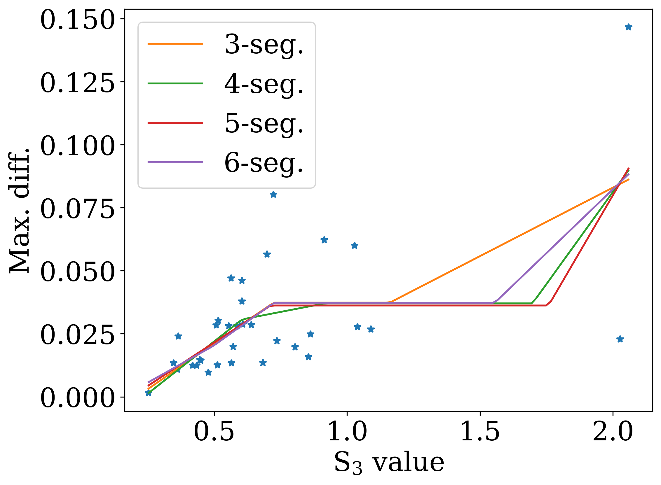
(b)

Figure 1: The maximal error in geometry optimization as a function of the $S_{2}$ value. (1(a)) The orange line corresponds to a piecewise linear fit to the data using four segments for the piecewise linear function. (1(b)) Piecewise linear fits to the data with a varying number of segments.

Aside from CC-based simulations, we can also perform MP2 simulations, and use the obtained doubles amplitudes to compute the $S$-diagnostics. We find that the proposed $S$-diagnostics correlate similarly well with MP2 based calculations as it does for CCSD, see Table 3

	$\Delta r_{\rm abs}^{\rm(max)}$	$\Delta r_{\rm abs}^{\rm(ave)}$	$\Delta r_{\rm rel}^{\rm(ave)}$
$S_{1}$	(0.55992, 0.000384)	(0.54569, 0.000577)	(0.49781, 0.002006)
$S_{2}$	(0.56687, 0.000313)	(0.54801, 0.000541)	(0.49858, 0.001968)
$S_{3}$	(0.55992, 0.000384)	(0.54569, 0.000577)	(0.49781, 0.002006)

Table 3: Spearman correlation between $S$-diagnostics computed from MP2 doubles amplitudes and different errors in geometry optimization.

4.2 Model Systems

In this section we investigate the use of the proposed $S$-diagnostics for four model systems whose multi-reference character can be controlled by simple geometric change: (1) twisting ethylene, (2) the C${}_{2\text{v}}$ insertion pathway for BeH₂ (Be $\cdots$ H₂) ²⁹, (3) the H₄ model (transition from square to linear geometry) ³⁰ (4) the H₄ model (symmetrically disturbed on a circle); the computations are performed in cc-pVTZ basis.

4.2.1 Twisting ethylene

We begin by numerically investigating the proposed $S$-diagnostics for ethylene twisted around the carbon–carbon bond, see Fig. 2.

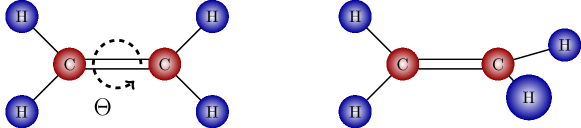
Figure 2: Depiction of the ethylene (C₂H₄) model with twist angle $\Theta$.

At a twist angle of 90°, this system shows a strong multi-reference character. This can be seen as follows: At the equilibrium geometry, i.e., in a planar geometry, the two carbon $p$ orbitals are perpendicular to the molecular plane form bonding $\pi$ and anti-bonding $\pi^{*}$ orbitals. In this geometry, the ground state doubly occupies the $\pi$-orbital. As we twist around the carbon–carbon bond, the overlap between the two $p$ orbitals decreases and becomes zero at 90°. Therefore, at 90° the $\pi$ and $\pi^{*}$ orbitals become degenerate and the $\pi$-bond is broken. This (quasi) degeneracy can also be observed numerically by computing the HOMO-LUMO gap as a function of the twist angle, see Fig. 3(a). Computing the corresponding ground state energy as a function of the twist angle, we observe the characteristic energy cusp at exactly 90°, see Fig. 3(b).

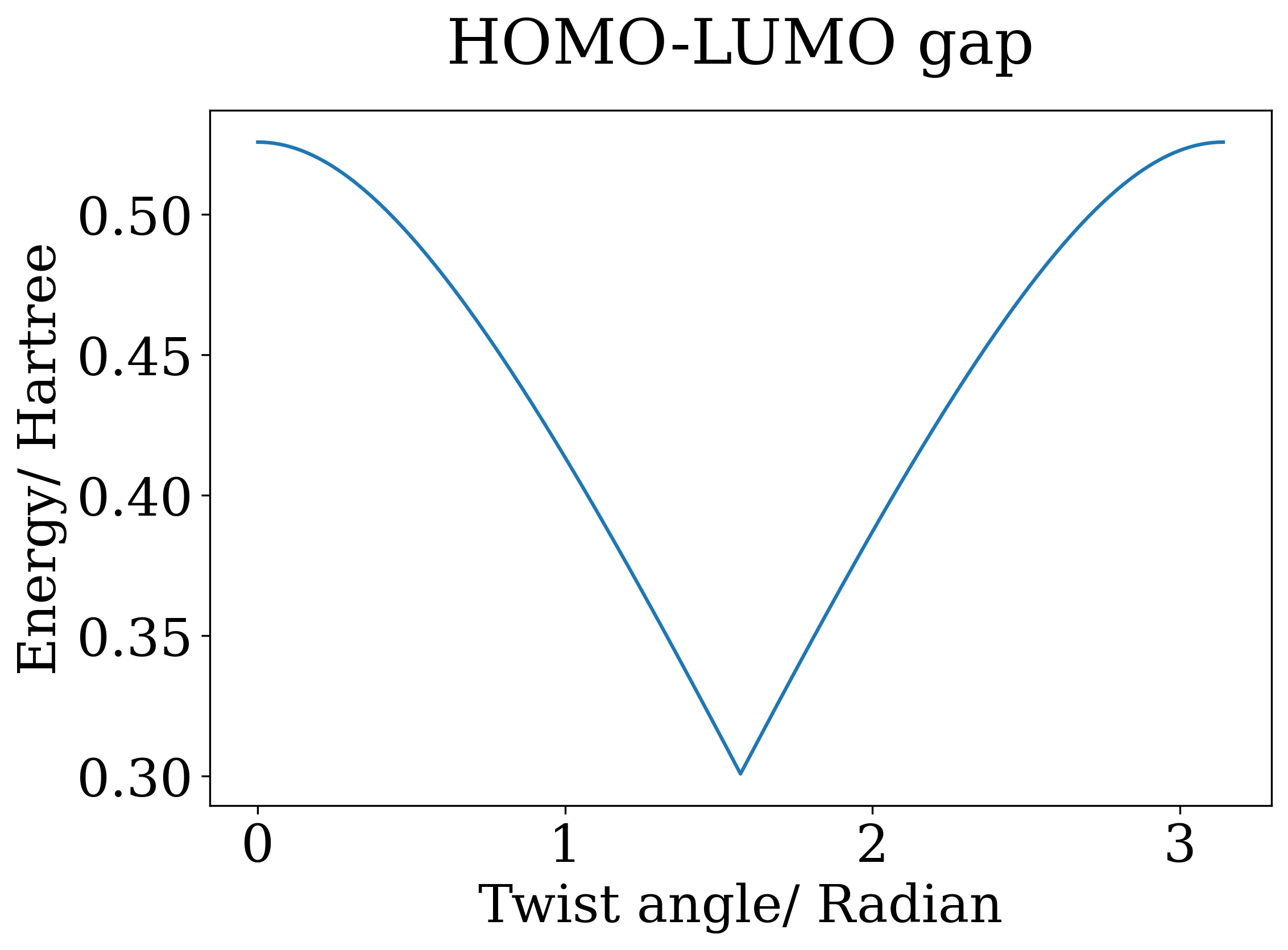
(a)

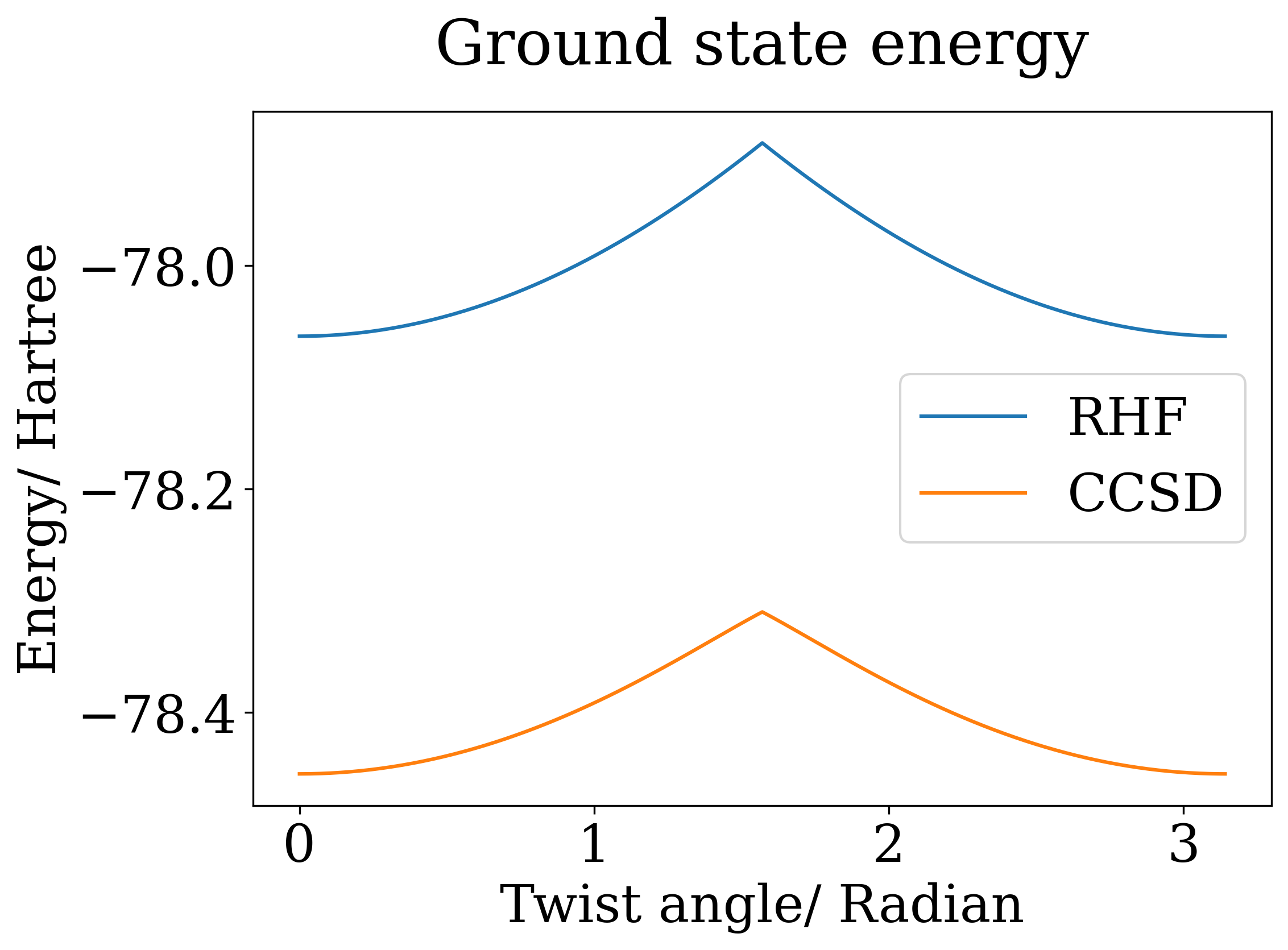
(b)

Figure 3: (3(a)) HOMO-LUMO gap of C₂H₄ as a function of the twist angle (3(b)) RHF and RCCSD energies of C₂H₄ as a function of the twist angle

Due to the quasi degeneracy around 90°, we compare the $S$-diagnostic with the MRI index suggested in Ref. 8. We clearly see the indication of the quasi degeneracy in the MRI index, see Fig. 4(b). The $S$-diagnostic also indicates the problematic region around 90°. By numerical comparison, we find that a cut-off value of $v_{\rm crit}^{(2)}=1.9$ and $v_{\rm crit}^{(3)}=1.8$ for $S_{2}$ and $S_{3}$, respectively, indicates the same region of quasi degeneracy as the MRI index.

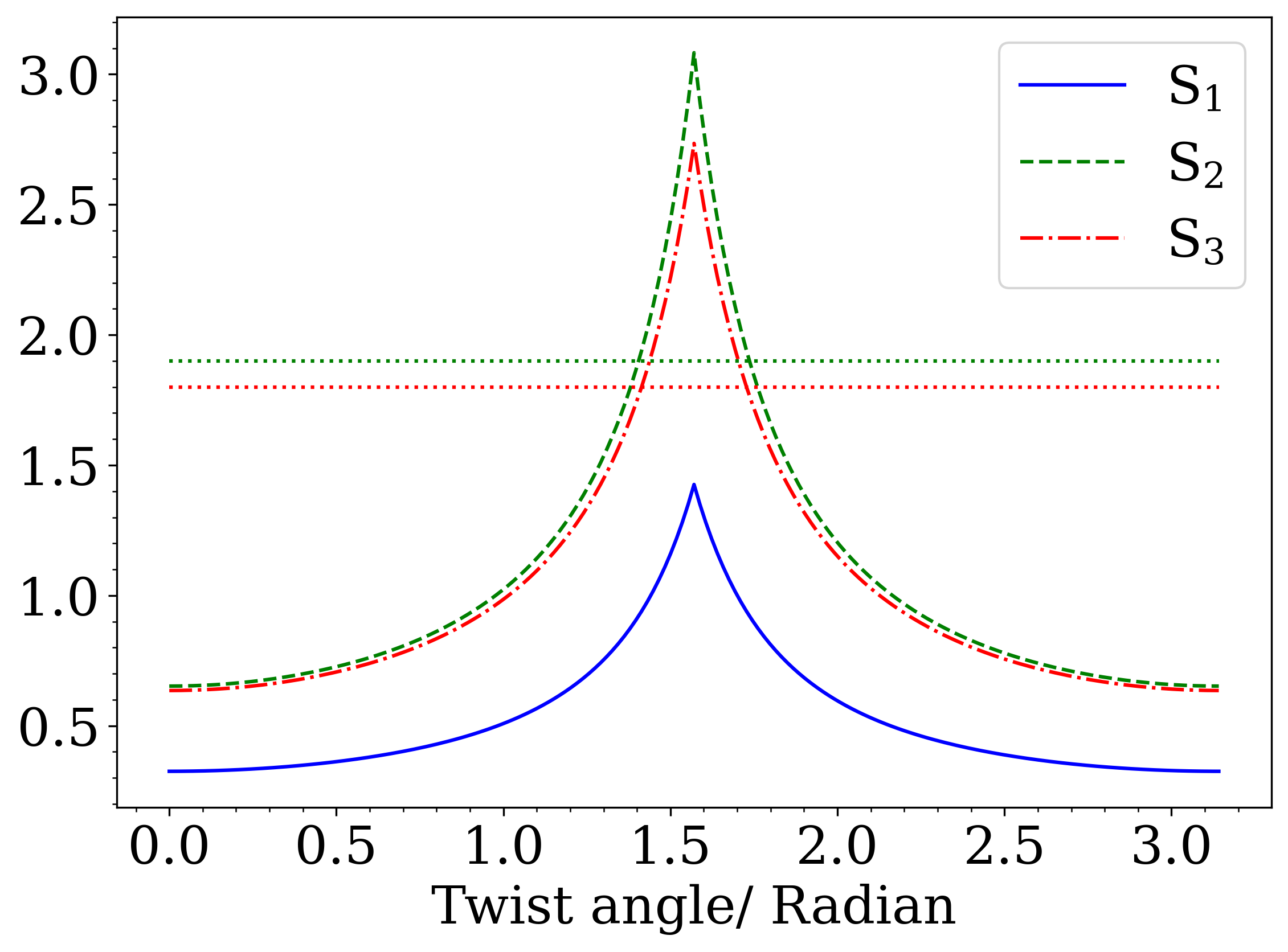
(a)

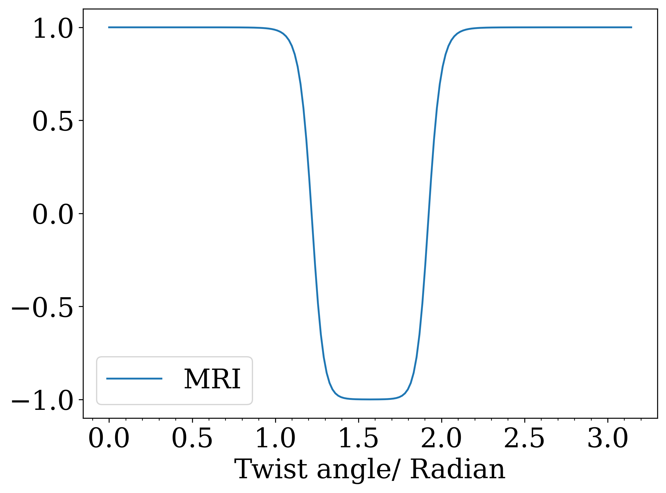
(b)

Figure 4: (4(a)) The proposed $S$-diagnostics of C₂H₄ as a function of the twist angle, the dotted green and red horizontal lines correspond to $v_{\rm crit}^{(2)}=1.9$ and $v_{\rm crit}^{(3)}=1.8$, respectively. (4(b)) The previously suggested MRI of C₂H₄ as a function of the twist angle

4.2.2 C_2v insertion pathway for BeH₂

Next we shall investigate the C_2v insertion pathway for BeH₂ (Be $\cdots$ H₂) ²⁹. The model represents an insertion of the Be atom into the H₂ molecule. The transformation coordinate connects the non-interacting subsystems (Be + H₂) with the linear equilibrium state (H-Be-H), see Fig. 5

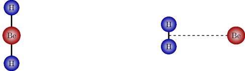
Figure 5: Depiction of the C_2v insertion pathway for BeH₂.

We here follow the insertion pathway outlined in Ref. 29 and denote the position of the beryllium atom by X-position, where X-position equal to zero corresponds to the linear equilibrium state and X-position equal to five corresponds to the non-interacting subsystems. The transition state of this chemical transformation has a pronounced multi-reference character. Another distinguishing feature of this model system is a change in the character of the dominating determinant in the wave function along the potential energy surface. There are two leading determinants in the wave function, each of which dominates in a certain region of the potential energy surface while both are quasi-degenerate around the transition-state geometry. This leads yields to discontinuities as can be seen in Figs. 6(b) and 6(a)

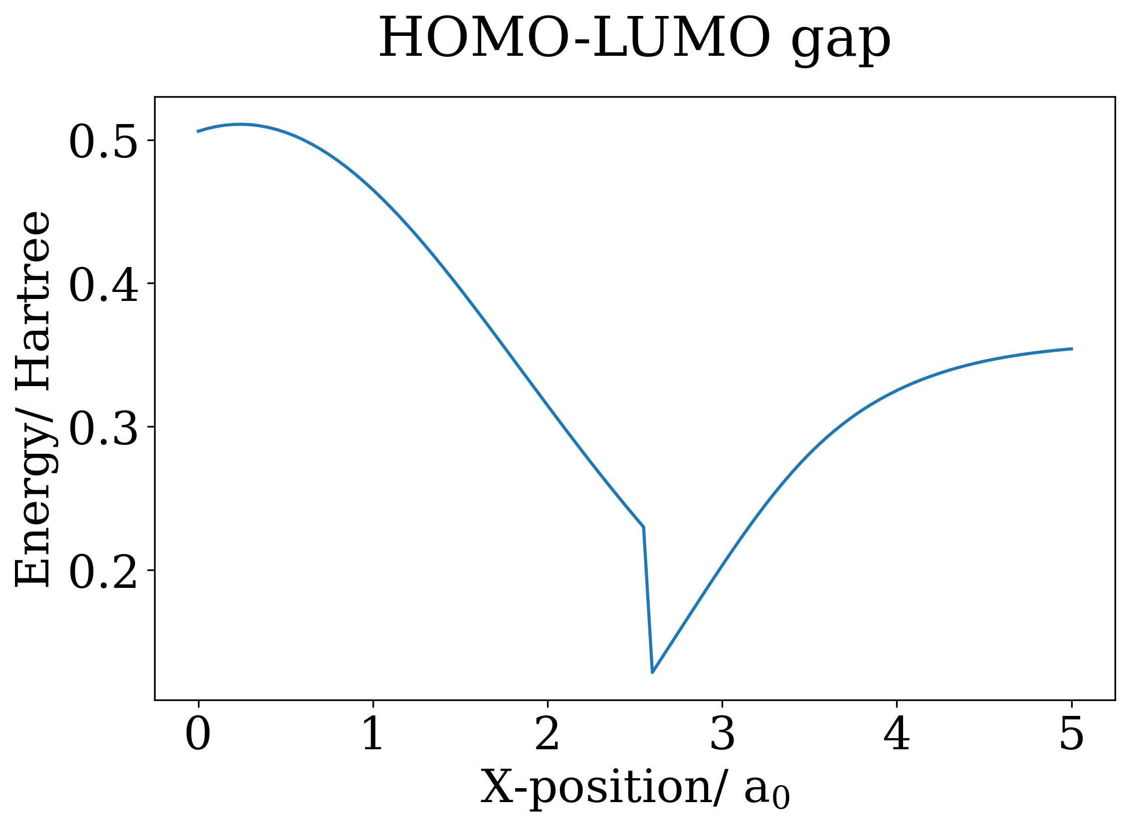
(a)

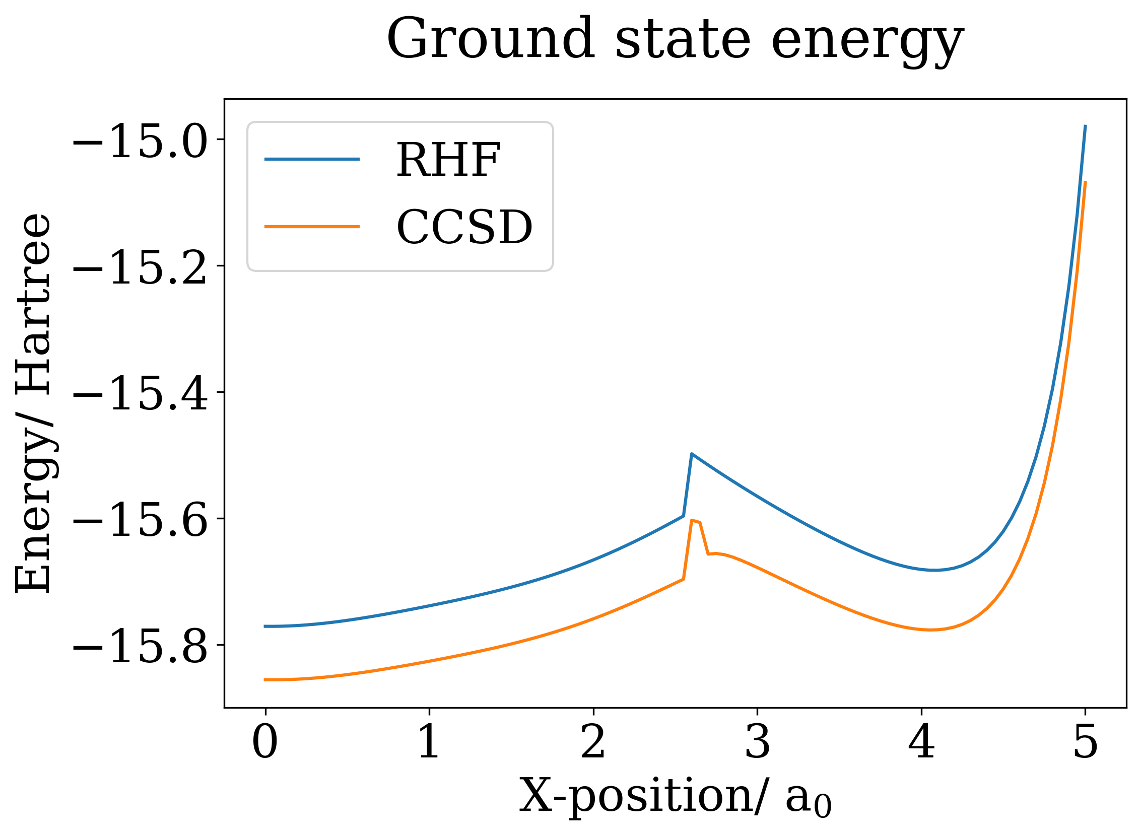
(b)

Figure 6: (6(a)) HOMO-LUMO gap as a function of the $X$-position (6(b)) RHF and RCCSD energies as a function of the $X$-position.

Due to the quasi-degeneracy that appears along the transition path, we again compare the proposed $S$-diagnostics with the MRI index suggested in Ref. 8. We clearly see the indication of the quasi degeneracy in the MRI index, see Fig. 7(b). The region indicated by MRI$<-0.99$ corresponds to $x\in[2.6,3.05]$. The $S$-diagnostic also indicates a region where the CC computations are potentially unreliable. It is worth mentioning that choosing the critical values similar to the previous example, i.e., $v_{\rm crit}^{(2)}=1.9$ and $v_{\rm crit}^{(3)}=1.8$, the predicted region corresponds to $x\in[2.5,4.5]$ and $x\in[2.5,4.25]$, respectively. In order to reproduce the same region of quasi-degeneracy as indicated by the MRI index, the critical values have to be adjusted to $v_{\rm crit}^{(2)}=3.8$ and $v_{\rm crit}^{(3)}=3.5$, respectively.

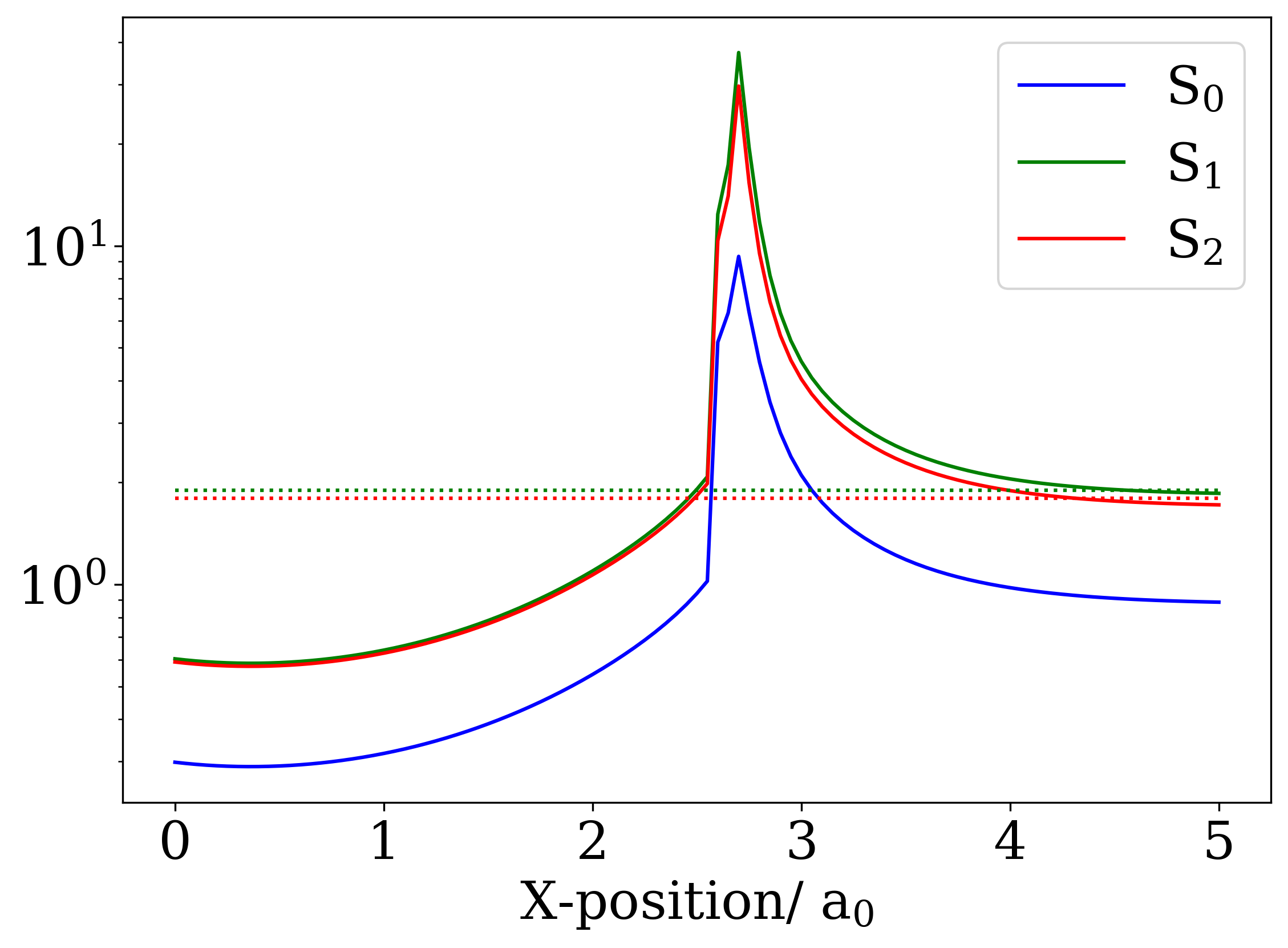
(a)

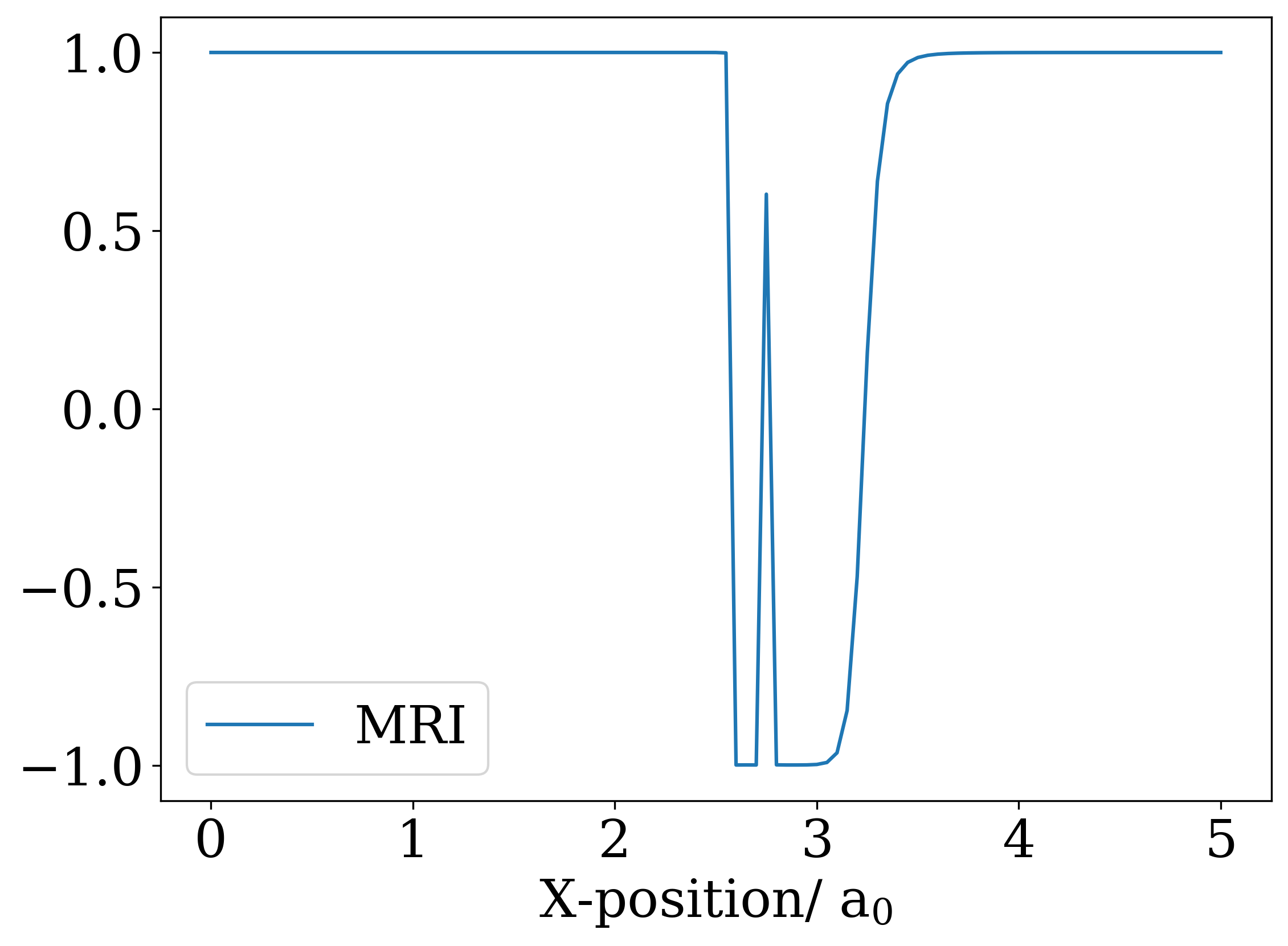
(b)

Figure 7: (7(a)) shows the $S$-diagnostics, the dotted green, and red horizontal lines correspond to $v_{\rm crit}^{(2)}=1.9$ and $v_{\rm crit}^{(3)}=1.8$, respectively. (7(b)) shows the previously suggested MRI

4.2.3 H₄ model (transition from square to linear geometry)

Next, we shall investigate the proposed $S$-diagnostics applied to the H₄ model. The H₄ model is a standard transition model that allows steering the quasi-degeneracy using a single parameter, namely, the transition angle $\alpha$ where $\alpha=0$ corresponds to a square geometry and $\alpha=\pi/2$ corresponds to a linear geometry. Following Ref. ³⁰, we set a = 2.0 (a.u.), see Fig. 8.

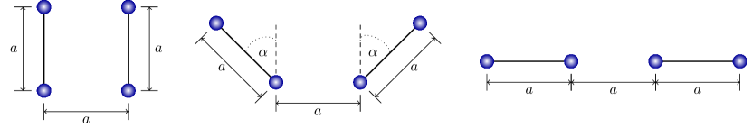
Figure 8: Depiction of the H₄ model undergoing the transition from a square geometry to linear geometry model by the angle $\alpha$.

We see that as the transition angle $\alpha$ tends to zero, the HOMO-LUMO gap closes and the system shows signs of (quasi-) degeneracy, see Fig. 9(a)

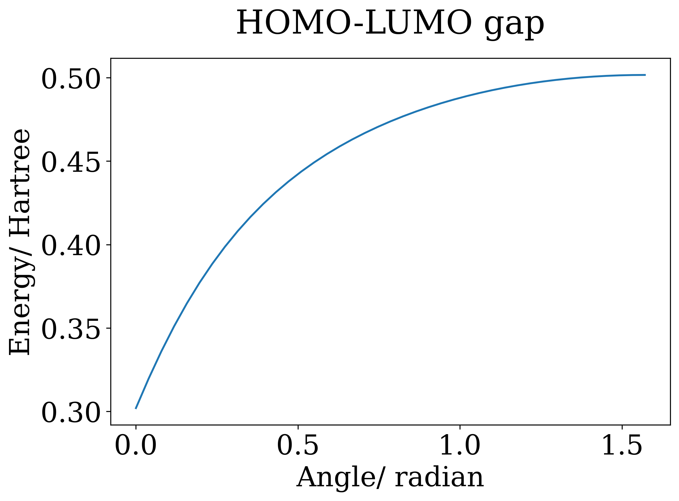
(a)

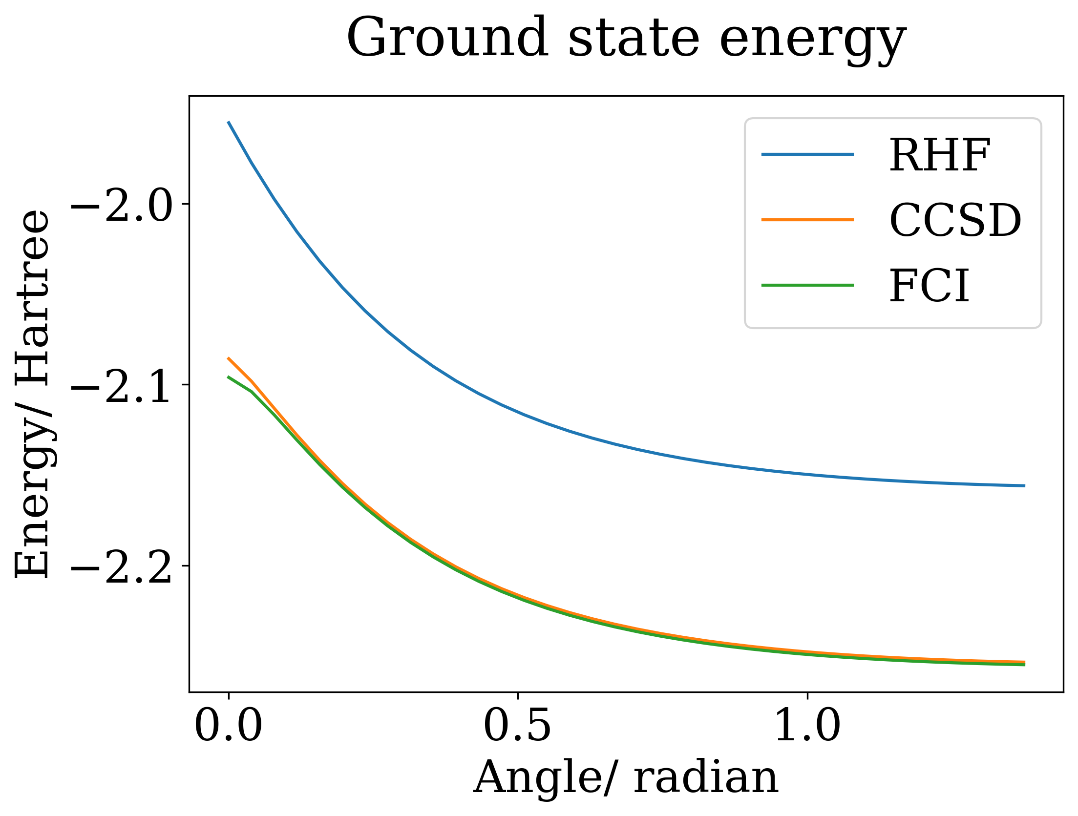
(b)

Figure 9: (9(a)) HOMO-LUMO gap of H₄ as a function of the transition angle (9(b)) RHF, CCSD and FCI energies of H₄ as a function of the transition angle

Due to the quasi degeneracy near $\alpha=0$, we again compare the proposed $S$-diagnostics with the MRI index. We clearly see the indication of the quasi degeneracy in the MRI index, see Fig. 10(b). The $S$-diagnostic also indicates the problematic region near zero transition angle. A cut-off value of $v_{\rm crit}^{(2)}=1.9$ and $v_{\rm crit}^{(3)}=1.8$ results in $S_{2}$ and $S_{3}$, respectively, indicating the same region of quasi degeneracy as the MRI index.

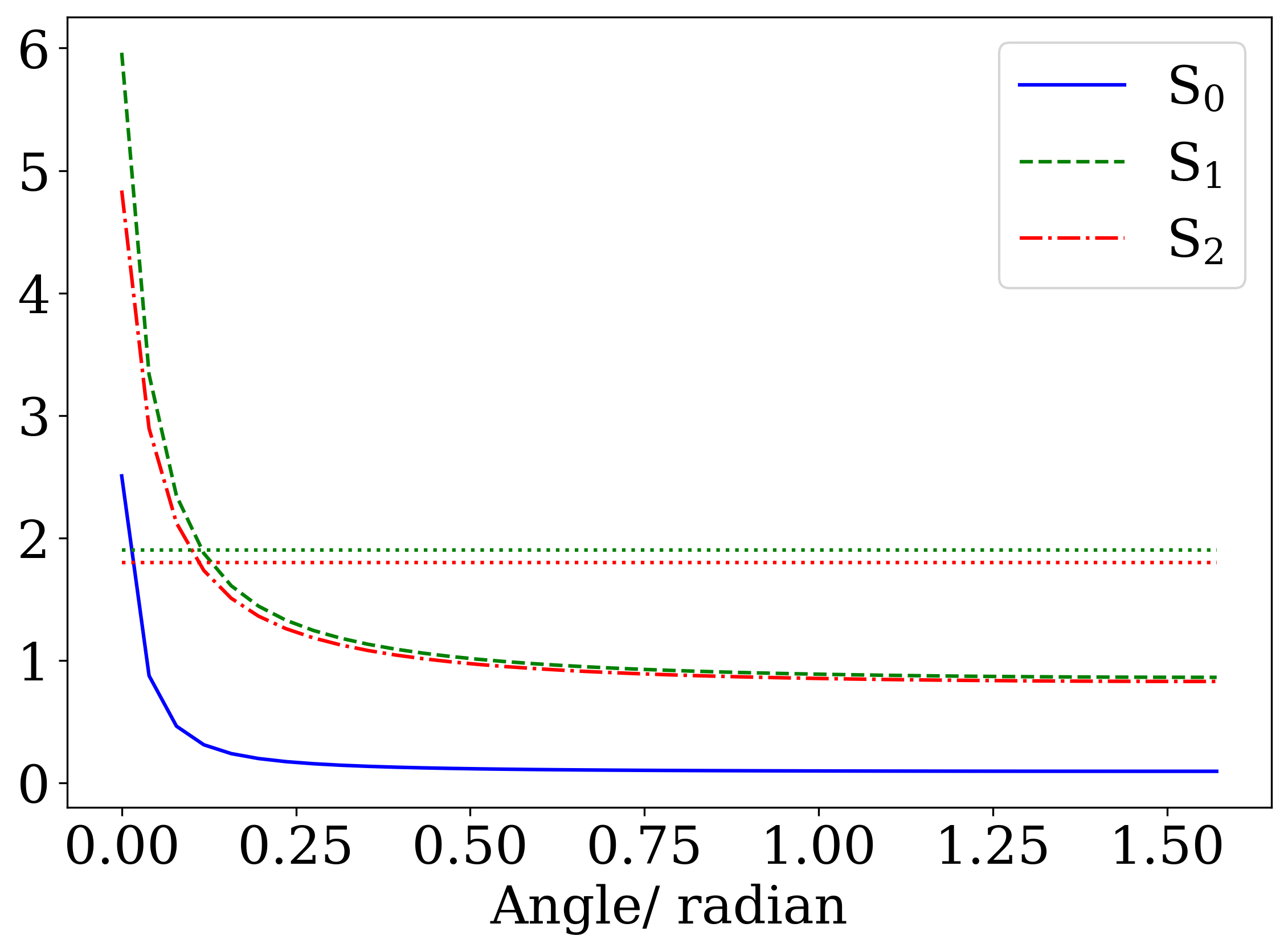
(a)

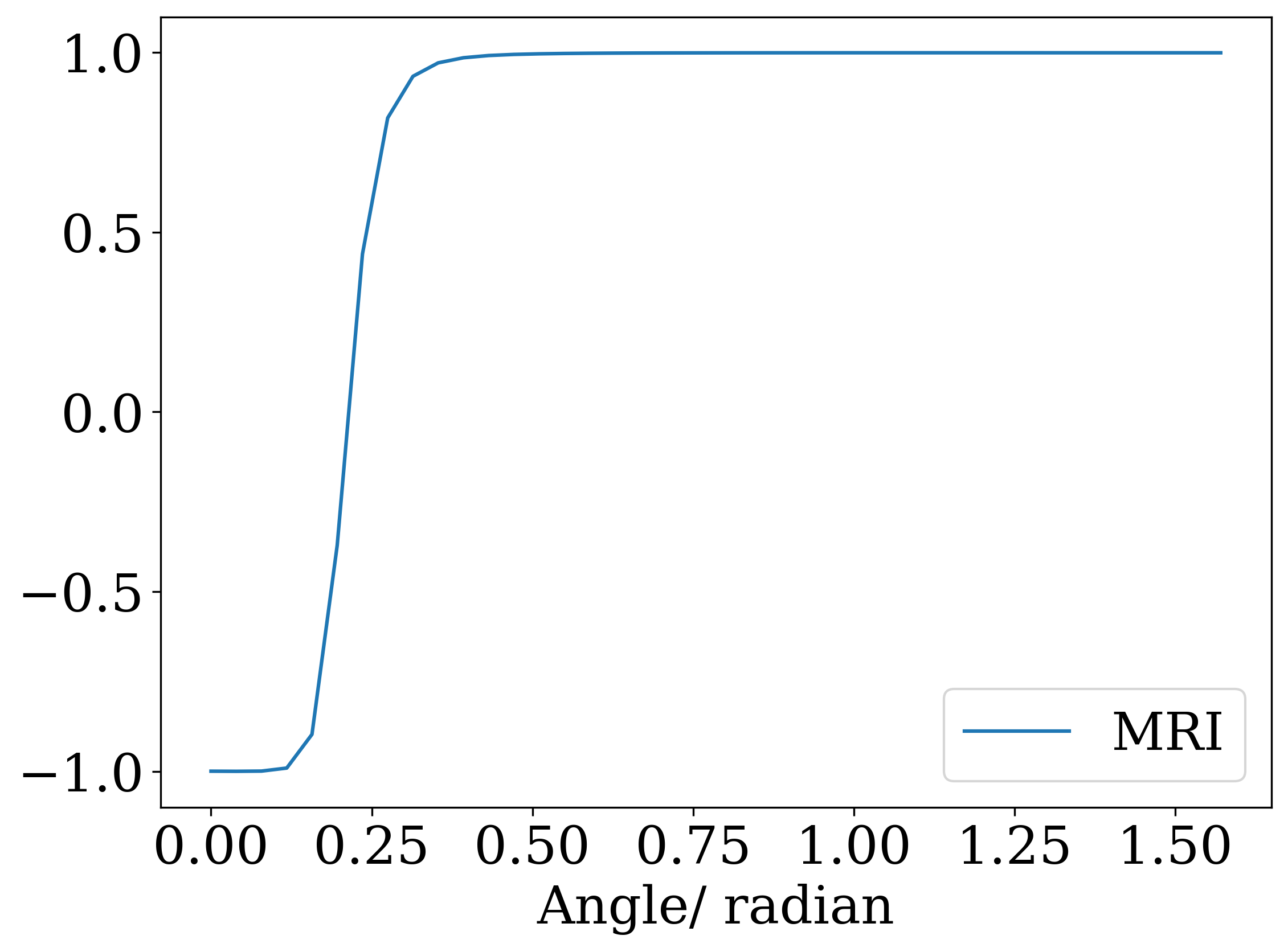
(b)

Figure 10: (10(a)) The $S$-diagnostics of H₄ as a function of the transition angle, the dotted green, and red horizontal lines correspond to $v_{\rm crit}^{(2)}=1.9$ and $v_{\rm crit}^{(3)}=1.8$, respectively. (10(b)) The previously suggested MRI of H₄ as a function of the transition angle.

For this small model Hamiltonian, it is moreover feasible to perform computations at the FCI level of theory, see Fig. 12. This comparison yields a quantitative comparison of error and $S$-diagnostic.

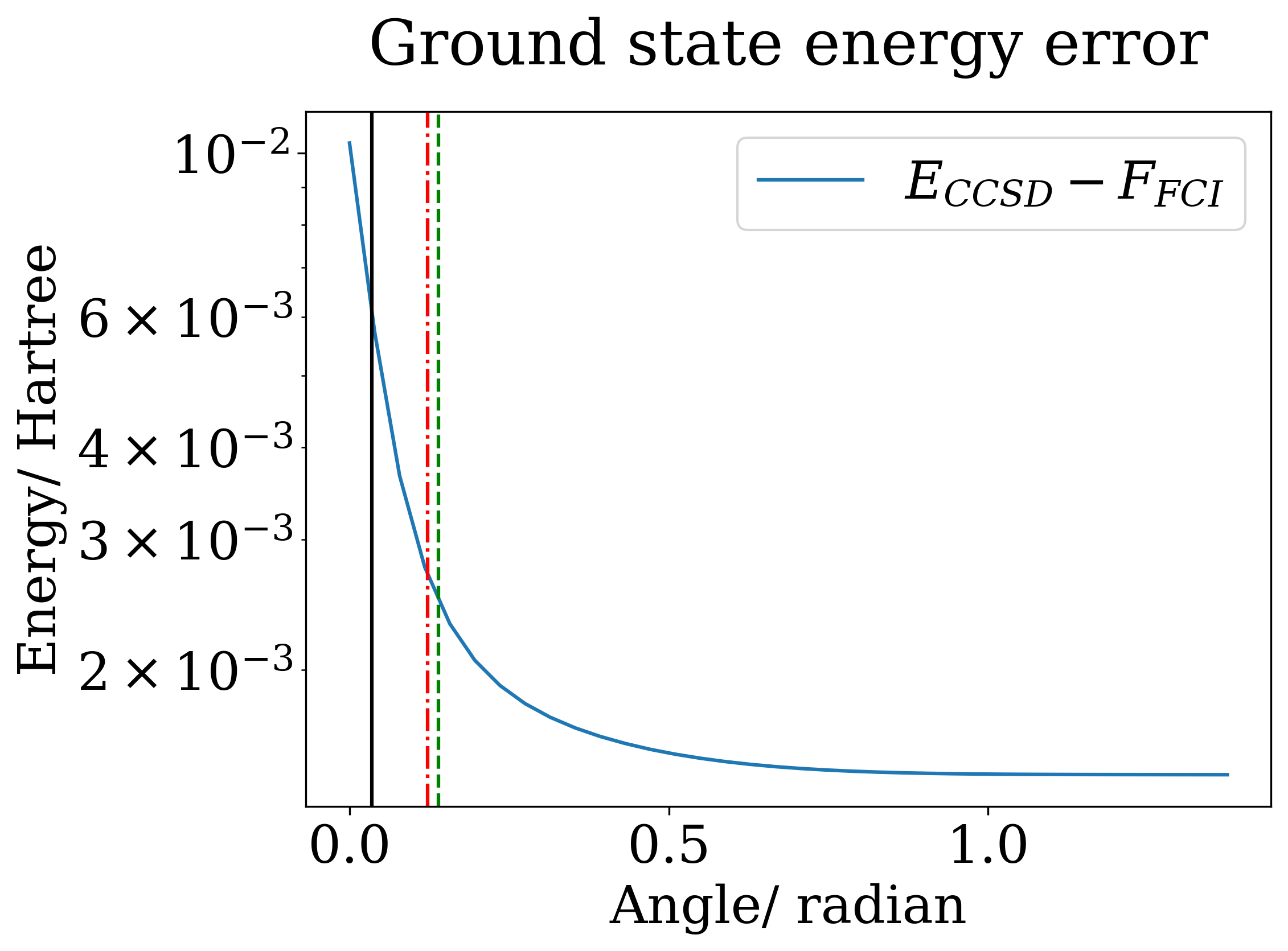
Figure 11:

Figure 12: The energy error of CCSD compared to the FCI reference energy using semi-log scales. The area left of the vertical solid (black), dashed (green), and dotted-dashed (red) lines correspond to the regions where the MRI, $S_{2}$, and $S_{3}$ diagnostic indicate a potential failure of CCSD, respectively.

4.2.4 H₄ model (symmetrically disturbed on a circle)

Another variant of the H₄ model that is commonly employed to evaluate CC methods consists of four hydrogen atoms symmetrically distributed on a circle of radius $R=1.738$ Å ³¹. For small or large angles, the system resembles two H₂ molecules that are reasonably well separated, but as the angle passes through $90\textdegree$, the four atoms form a square yielding a degenerate ground state. The exact energy is smooth as a function of the angle, but at the RHF level, we observe a cusp at $90\textdegree$, similar to the rotation of the carbon-carbon bond in ethylene. We follow the system’s geometry configuration outlined in Ref. ³², see Fig. 13.

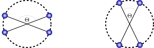
Figure 13: Depiction of the H₄ model undergoing a symmetric disturbance on a circle modeled by the angle $\Theta$.

We see that as the transition angle $\Theta$ tends to $\pi/2$ radians (90°), the HOMO-LUMO gap closes and the system shows signs of (quasi) degeneracy, see Fig. 14(a)

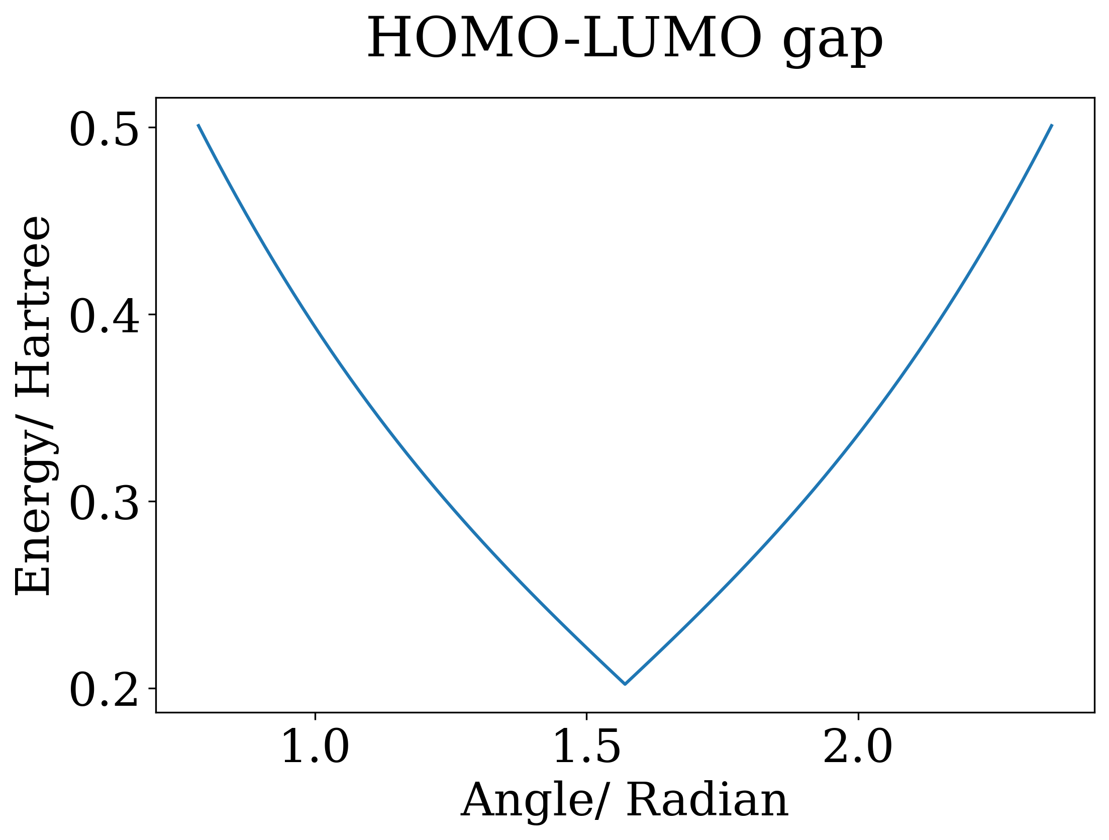
(a)

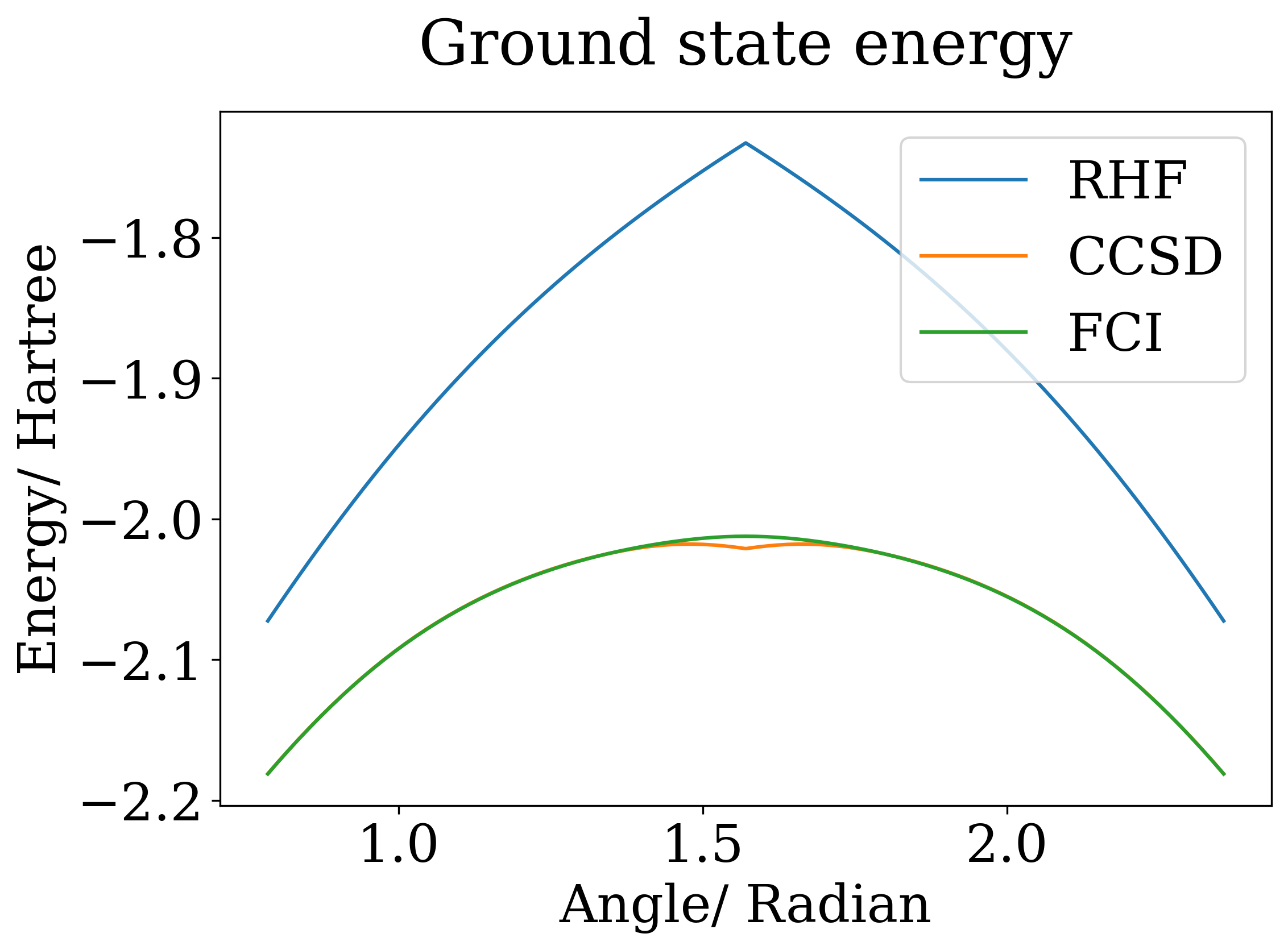
(b)

Figure 14: (14(a)) HOMO-LUMO gap of H₄ as a function of the transition angle (9(b)) RHF, RCCSD energies of H₄ as a function of the transition angle.

Due to the quasi degeneracy near $\Theta=\pi/2$ (90°), we again compare the proposed $S$-diagnostics with the MRI index. We clearly see the indication of the quasi degeneracy in the MRI index, see Fig. 15(b). The $S$-diagnostic also indicates the problematic region near zero transition angle. A cut-off value of $v_{\rm crit}^{(2)}=1.9$ and $v_{\rm crit}^{(3)}=1.8$ results in $S_{2}$ and $S_{3}$, respectively, indicating the same region of quasi degeneracy as the MRI index.

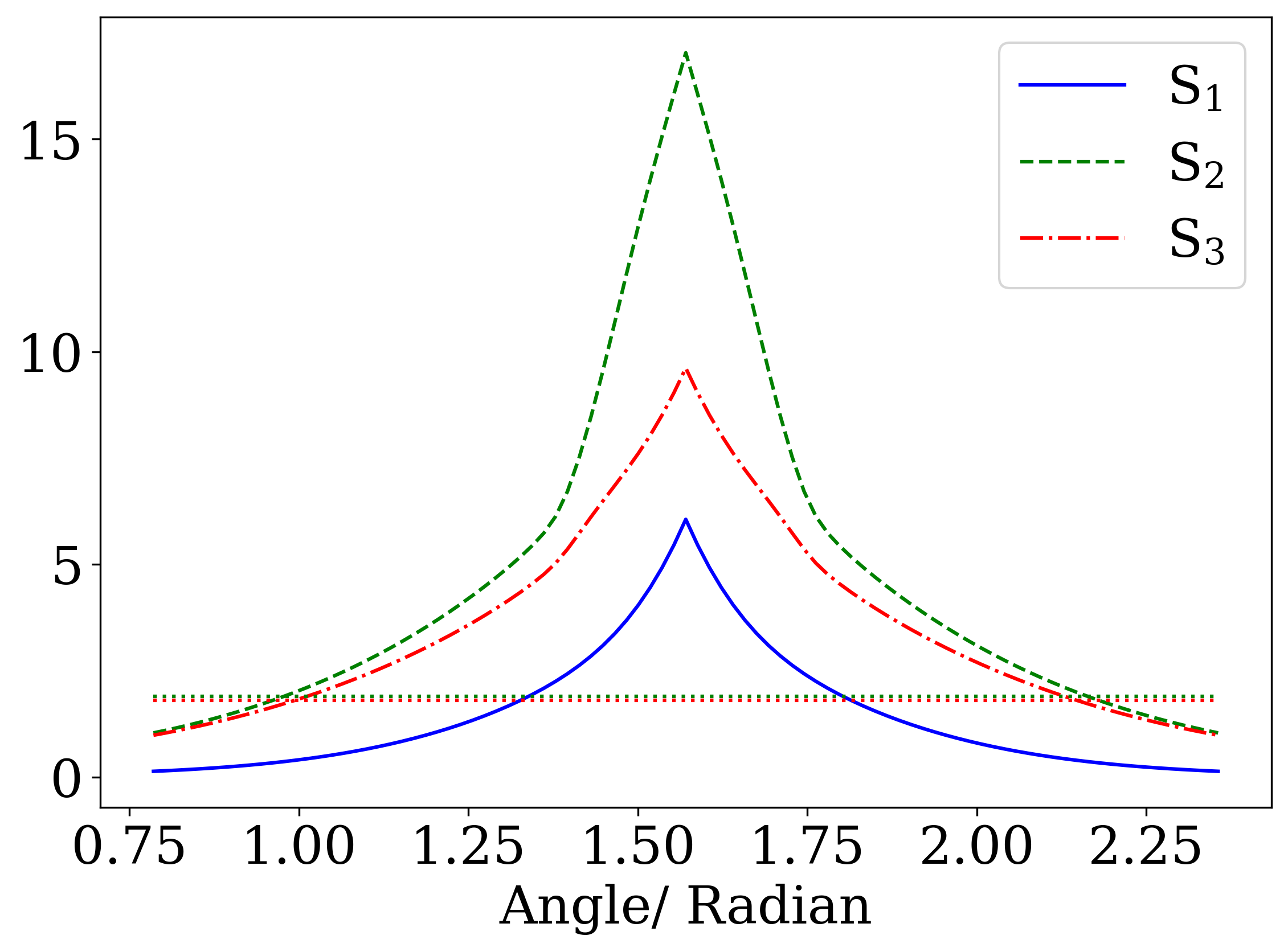
(a)

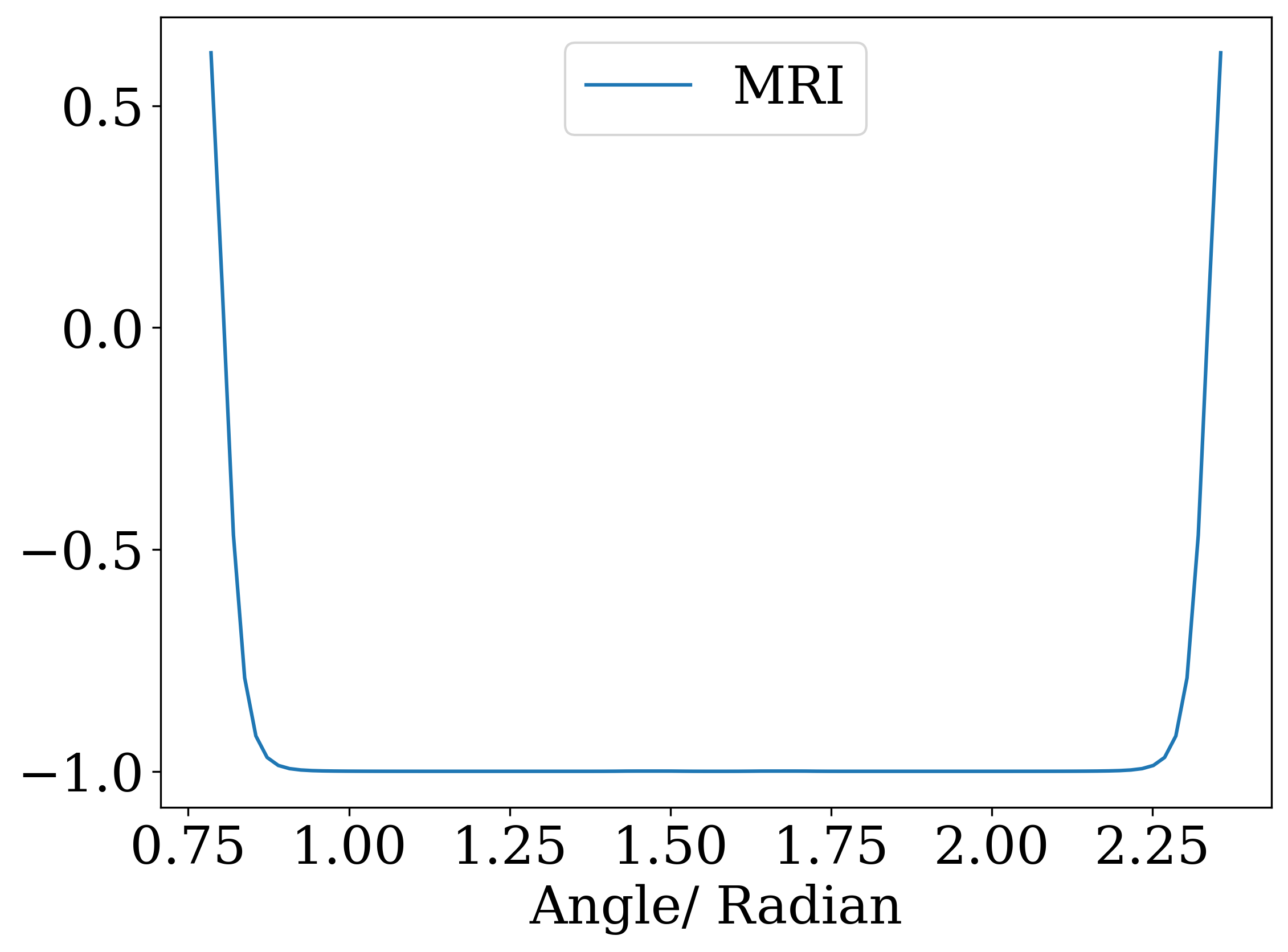
(b)

Figure 15: (15(a)) The $S$-diagnostics of H₄ as a function of the transition angle, the dotted green, and red horizontal lines correspond to $v_{\rm crit}^{(2)}=1.9$ and $v_{\rm crit}^{(3)}=1.8$, respectively. (15(b)) The previously suggested MRI of H₄ as a function of the transition angle.

For this small model Hamiltonian, it is moreover feasible to perform computations at the FCI level of theory, see Fig. 16. This comparison reveals the variational collapse of the CCSD energy, see Fig. 16(a), and moreover yields a quantitative comparison of error and $S$-diagnostic. The trusted region suggested by the $S$-diagnostic corresponds to a CCSD energy error smaller than $2\cdot 10^{-4}$ a.u. which is below the chemical accuracy threshold.

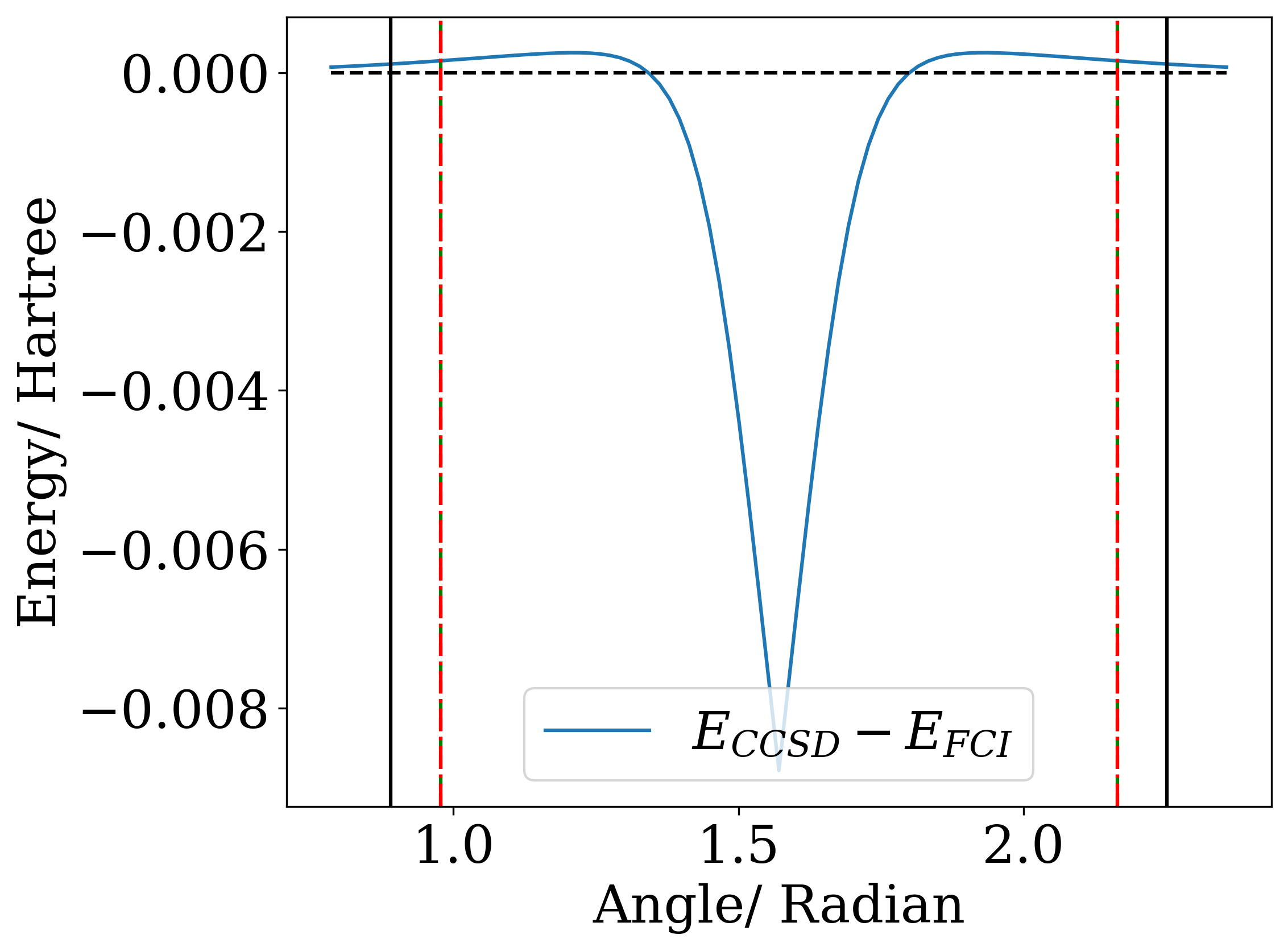
(a)

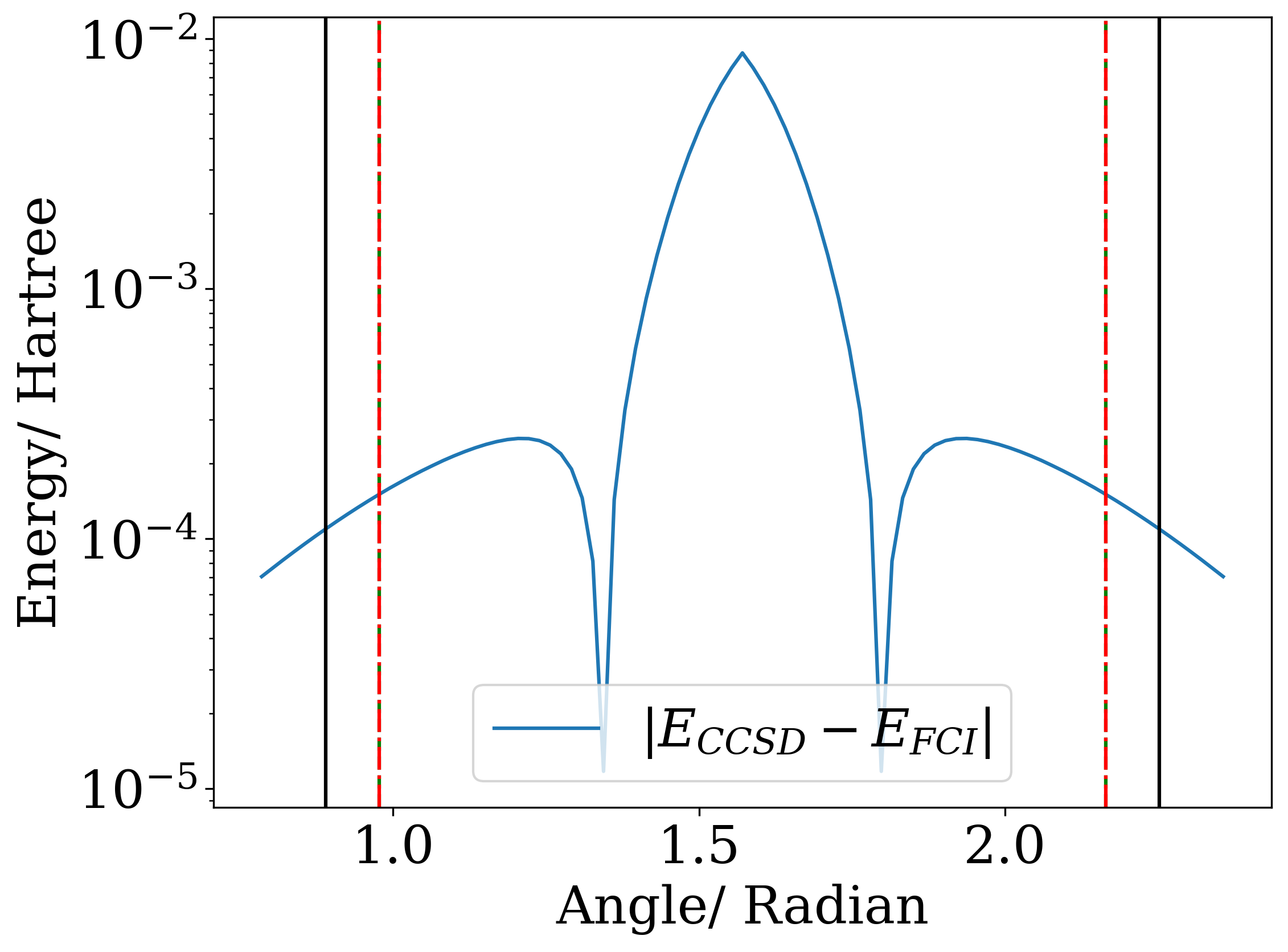
(b)

Figure 16: (16(a)) The energy error of CCSD compared to the FCI reference energy. Note that in the region of 1.3-1.8 radians the CCSD energy is lower than the FCI reference energy, which indicates the variational collapse of the CCSD energy in this region. (16(b)) The absolute value of the energy error of CCSD compared to the FCI reference energy using semi-log scales. The area between the vertical solid (black), dashed (green), and dotted-dashed (red) lines correspond to the regions where the MRI, $S_{2}$, and $S_{3}$ diagnostic indicate a potential failure of CCSD, respectively.

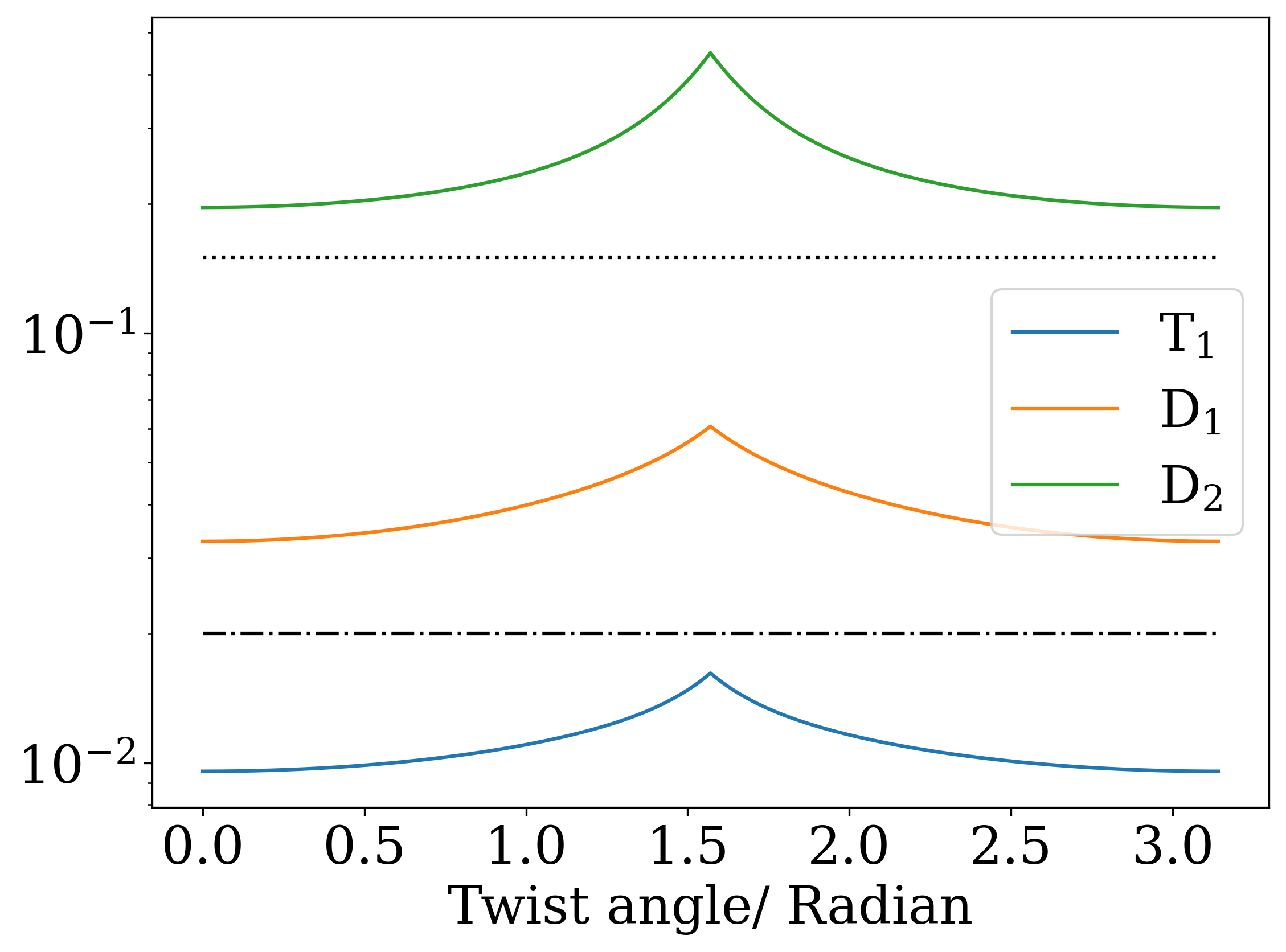
(b)

Figure 26: (26(a)) shows the $S$-diagnostics (26(b)) shows the previously suggested $T_{1}$, $D_{1}$ and $D_{2}$ diagnostics

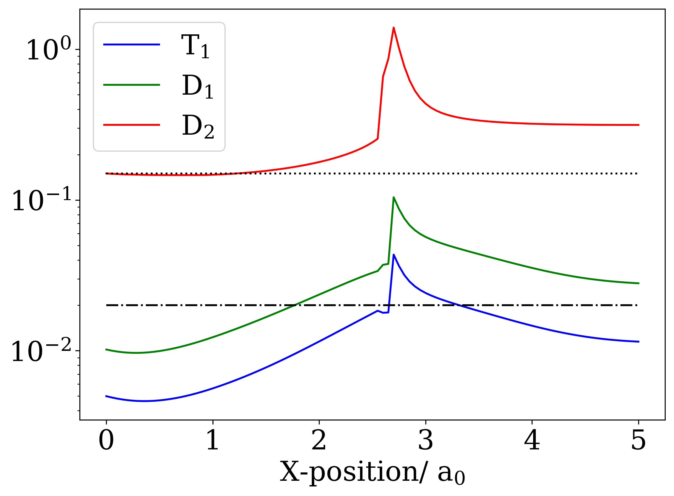
(b)

Figure 27: (27(a)) shows the $S$-diagnostics (27(b)) shows the previously suggested $T_{1}$, $D_{1}$ and $D_{2}$ diagnostics

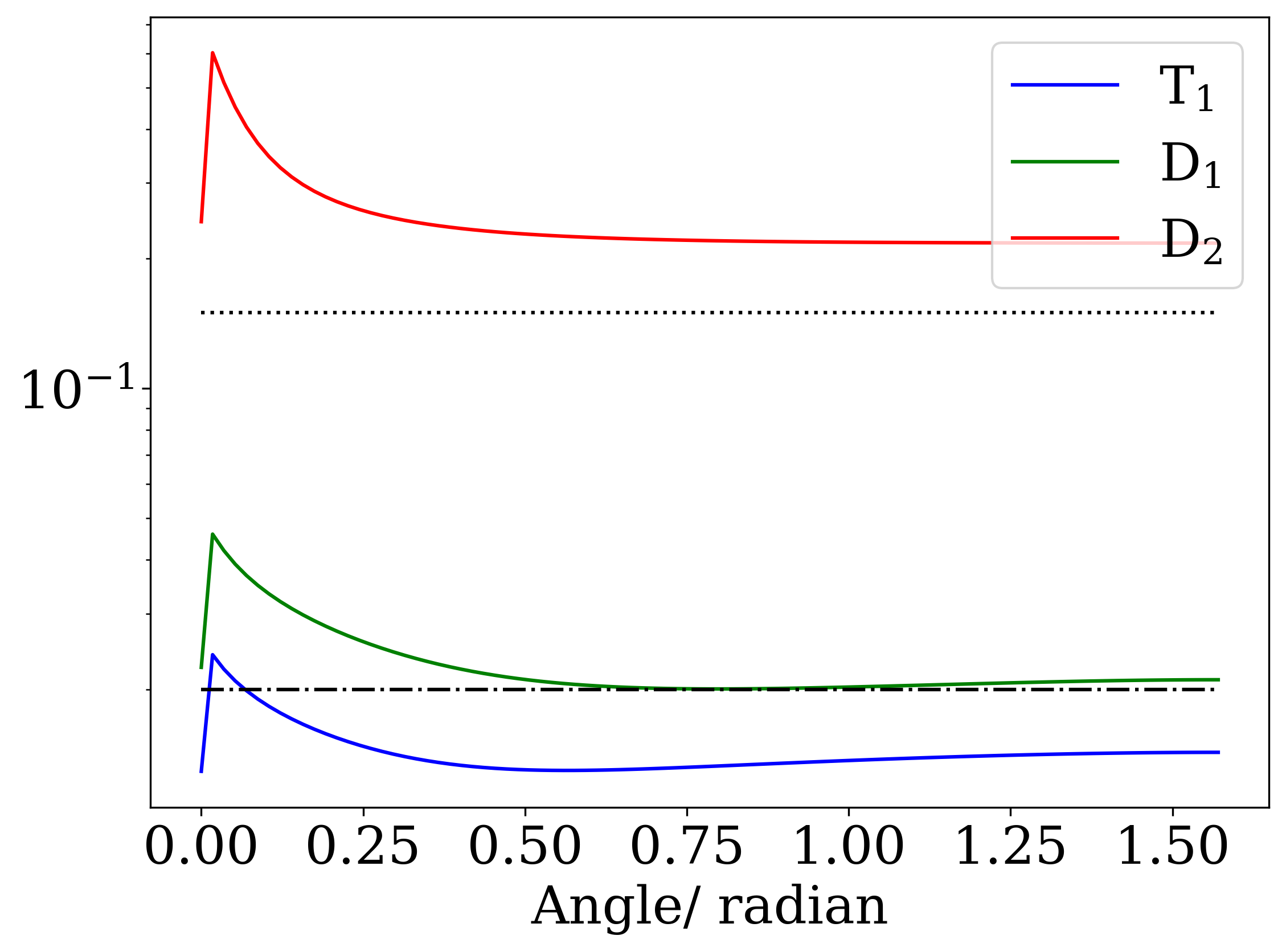
(b)

Figure 28: (28(a)) shows the $S$-diagnostics (28(b)) shows the previously suggested $T_{1}$, $D_{1}$ and $D_{2}$ diagnostics

Since the simulations performed in the previous section suggest that the previously used $T_{1}$, $D_{1}$, and $D_{2}$ diagnostics are uncorrelated, or merely weakly correlated, we do not report their performance here. The computations showing the performance of the $T_{1}$, $D_{1}$, and $D_{2}$ diagnostics can be found in the Appendix, see Figs. 26, 27, 28 and 29

4.3 Transition metal complexes

In this section we investigate three square-planar copper complexes [CuCl₄]^2-, [Cu(NH₃)₄]²⁺, and [Cu(H₂O)₄]²⁺. Transition metal complexes are in general considered to be strongly correlated systems and complete active space self-consistent field (CASSCF) theory is commonly applied, with multi-reference perturbation or truncated CI corrections for dynamic correlation. However, as shown in Ref. 7, the single reference CC method performs very well despite the large $D_{1}$ diagnostic value. We use these systems to scrutinize the proposed $S$-diagnostics for larger systems that are known to be misleadingly diagnosed by the $D_{1}$ diagnostics.

Similar to Ref. 7, we perform the simulation of [CuCl₄]^2-, [Cu(NH₃)₄]²⁺, and [Cu(H₂O)₄]²⁺ in 6-31G basis using UHF and ROHF as reference states. Also, He, Ne, and Ar cores were frozen in the nitrogen, chlorine, and copper atoms, respectively, resulting in 41 electrons in 50, 66, and 74 orbitals for the [CuCl₄]^2-, [Cu(H₂O)₄]²⁺, and [Cu(NH₃)₄]²⁺ molecules, respectively. We list the ground state energies obtained at the mean-field level of theory and the corresponding CCSD results in Table 4; we moreover list the HOMO-LUMO gap which enters in the $S$-diagnostics.

	UHF	$\gamma_{UHF}$	UCCSD	RHOF	$\gamma_{ROHF}$	UCCSD
[CuCl4]2-	-3476.764	0.453	-3477.119	-3476.763	0.146	-3477.119
[Cu(NH3)4]2+	-1862.977	0.564	-1863.663	-1862.976	0.351	-1863.663
[Cu(H2O)4]2+	-1942.225	0.677	-1942.914	-1942.224	0.340	-1942.914

Table 4: Energies values and HOMO-LUMO gap obtained with UHF, ROHF, and UCCSD calculations given the reference state from UHF and ROHF, respectively.

The results in Table 4 show that UHF and ROHF calculations predict similar energy values. Moreover, using the UHF, or ROHF reference state results in similar CCSD energy values. It is worth noticing that ROHF yields a generally smaller HOMO-LUMO gap. Since the performed CCSD calculations differ in their reference, we can compute the $S$-diagnostics for both sets of calculations. The results obtained from a UHF and ROHF reference are listed in Table 5 and in Table 6, respectively.

	$S_{1}$	$S_{2}$	$S_{3}$	$T_{1}$	$D_{1}$	$D_{2}$
[CuCl4]2-	0.208	0.409	0.406	0.019	0.158	0.110
[Cu(NH3)4]2+	0.203	0.403	0.398	0.014	0.130	0.121
[Cu(H2O)4]2+	0.155	0.308	0.305	0.011	0.072	0.116

Table 5: $S$-diagnostics obtained for the three square-planar copper complexes [CuCl₄]^2-, [Cu(NH₃)₄]²⁺, and [Cu(H₂O)₄]²⁺ in spin unrestricted formulation with UHF reference.

We see that all $S$-diagnostic variants suggest that the CCSD calculations were successful, and do not require additional numerical confirmation. This is opposed to the $D_{1}$ diagnostics, which aligns with the results reported in Ref. 7.

	$S_{0}$	$S_{1}$	$S_{2}$	$T_{1}$	$D_{1}$	$D_{2}$
[CuCl4]2-	0.645	1.285	1.27	0.020	0.167	0.110
[Cu(NH3)4]2+	0.326	0.646	0.638	0.015	0.139	0.121
[Cu(H2O)4]2+	0.309	0.614	0.607	0.011	0.077	0.116

Table 6: $S$-diagnostics obtained for the three square-planar copper complexes [CuCl₄]^2-, [Cu(NH₃)₄]²⁺, and [Cu(H₂O)₄]²⁺ in spin unrestricted formulation with ROHF reference.

Similar to the results in Table 5, we see that all variants of the $S$-diagnostic suggest that the CCSD calculations were successful. However, it is worth noticing that the $S$-diagnostic values have increased compared to the values reported in Table 5.

5 Conclusion

In this article, we proposed three a posteriori diagnostics for single-reference CC calculations which we called $S$-diagnostics, due to their origin in the strong monotonicity analysis. Contrary to previously suggested CC diagnostics, the $S$-diagnostics are motivated by mathematical principles that have been used to analyze CC methods of different flavors in the past ^{9, 18, 19, 15, 33}.

We performed a set of geometry optimizations for small to medium-sized molecules in order to reveal the correlation between the $S$-diagnostics and the error in geometry from CCSD calculations. The test set comprised all molecules that were used in previous articles concerning CC diagnostics ^{3, 4, 5, 6}. Our investigations revealed that the $S$-diagnostics correlate well and with large statistical relevance with different errors in geometry. This yields a first estimate of the critical values for the $S$-diagnostics beyond which the computational results should be confirmed using further and more careful numerical investigations. The observed correlation between the $S$-diagnostics and the different errors in geometry are comparable to the recently suggested EEN index ⁸. A heuristic test revealed that the $S$-diagnostics also correlate well and with large statistical relevance with the error in geometry at the MP2 level of theory. This suggests that the $S$-diagnostics can also be used as an a posteriori diagnostic for MP2 calculations. Our numerical simulations moreover showed that diagnostics based on single excitation cluster amplitudes, i.e., $D_{1}$ and $T_{1}$, are uncorrelated to errors in geometry optimization.

Following we investigated the $S$-diagnostics for transition state models that undergo a transition from a region in which CC calculations are reliable to a regime where the CC calculations require further numerical investigations—in this case, due to (quasi-) degeneracy of the ground state. The $S$-diagnostic detects the corresponding regions of (quasi-) degeneracy well. In fact, its performance is comparable to the recently suggested MRI indicator—an a posteriori indicator for multi-reference character ⁸.

The last set of numerical simulations targeted transition metal complexes which have recently been carefully benchmarked ⁷. The previously performed benchmark calculations revealed that diagnostics based on single excitation amplitudes severely misdiagnose the performance of CCSD for these transition metal complexes. Our computations confirm this, and moreover, show that the $S$-diagnostic correctly confirms the accuracy of the CCSD results outlined in Ref. 7.

These carefully performed numerical investigations suggest that the $S$-diagnostic is a promising candidate for an a posteriori diagnostic for single-reference CC and MP2 calculations. To further confirm this, benchmarks on a larger set of molecules will be performed in the future. Moreover, since the mathematical analysis of the single-reference CC method generalizes to periodic systems as well, we believe that the $S$-diagnostic can moreover be applied to simulations of solids at the CC and MP2 level of theory.

Throughout our numerical investigations, we observe a subpar performance of the $T_{1}$ and $D_{1}$ diagnostics. This suggests that those diagnostics should once and for all be removed as a posteriori diagnostic tools for single-reference CC calculations.

6 Appendix

6.1 Correlation in Geometry Optimization

Since we can correlate three $S$-diagnostic variants with three error measures, we can in principle perform the piecewise linear fit that is presented in Section on Correlation in Geometry Optimization for nine different scenarios. We here present the piecewise linear fits which were not addressed in the above article.

6.1.1 S₁-diagnostic Correlations

(a)

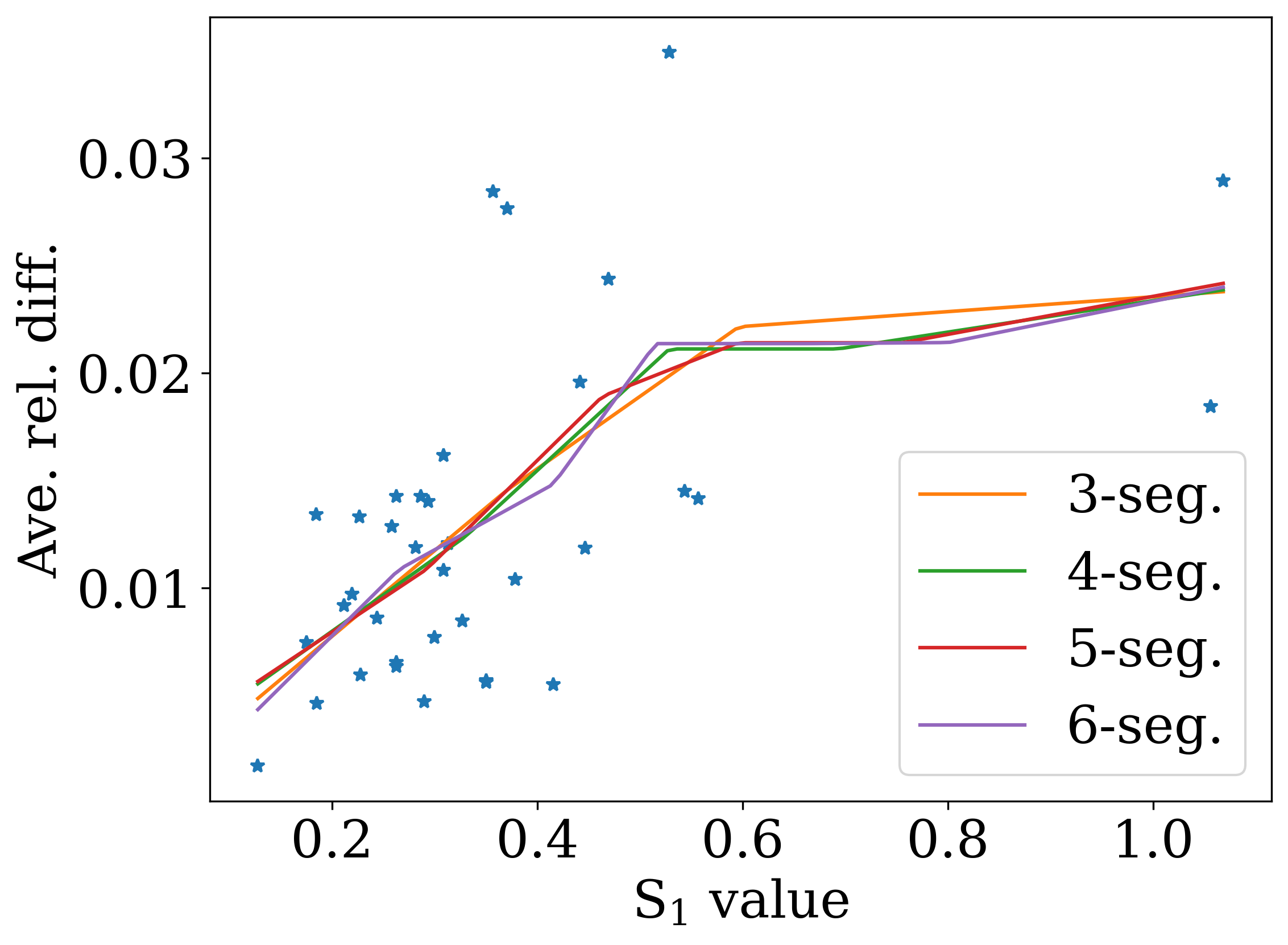
(b)

Figure 17: The averaged relative error in geometry optimization as a function of the $S_{1}$ value. (17(a)) The orange line corresponds to a piecewise linear fit to the data using four segments for the piecewise linear function. (17(b)) Piecewise linear fits to the data with a varying number of segments.

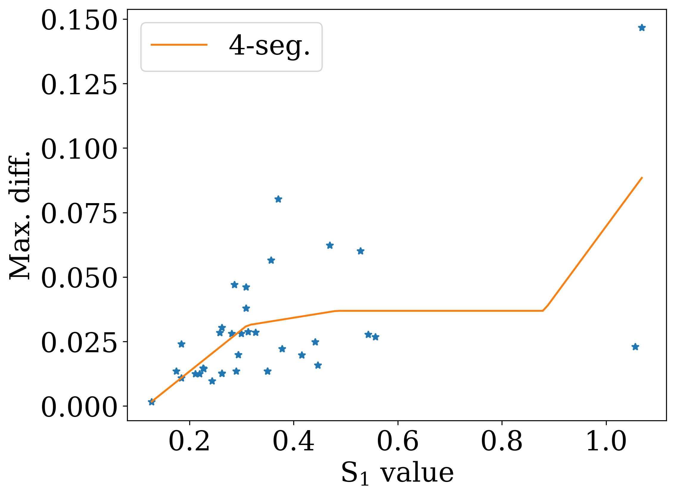
(a)

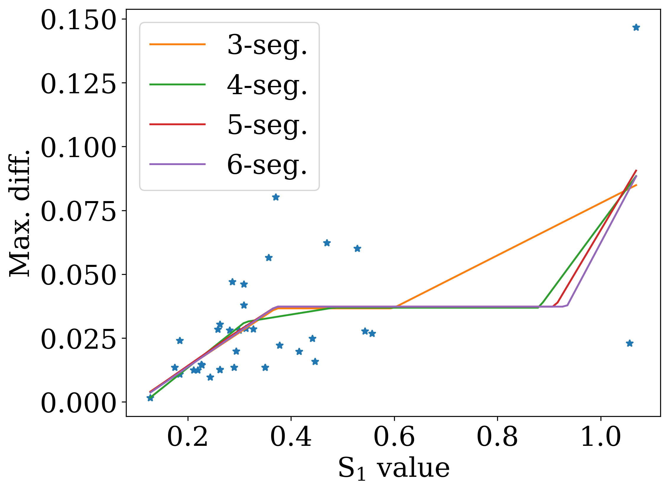
(b)

Figure 18: The maximal absolute error in geometry optimization as a function of the $S_{1}$ value. (18(a)) The orange line corresponds to a piecewise linear fit to the data using four segments for the piecewise linear function. (18(b)) Piecewise linear fits to the data with a varying number of segments.

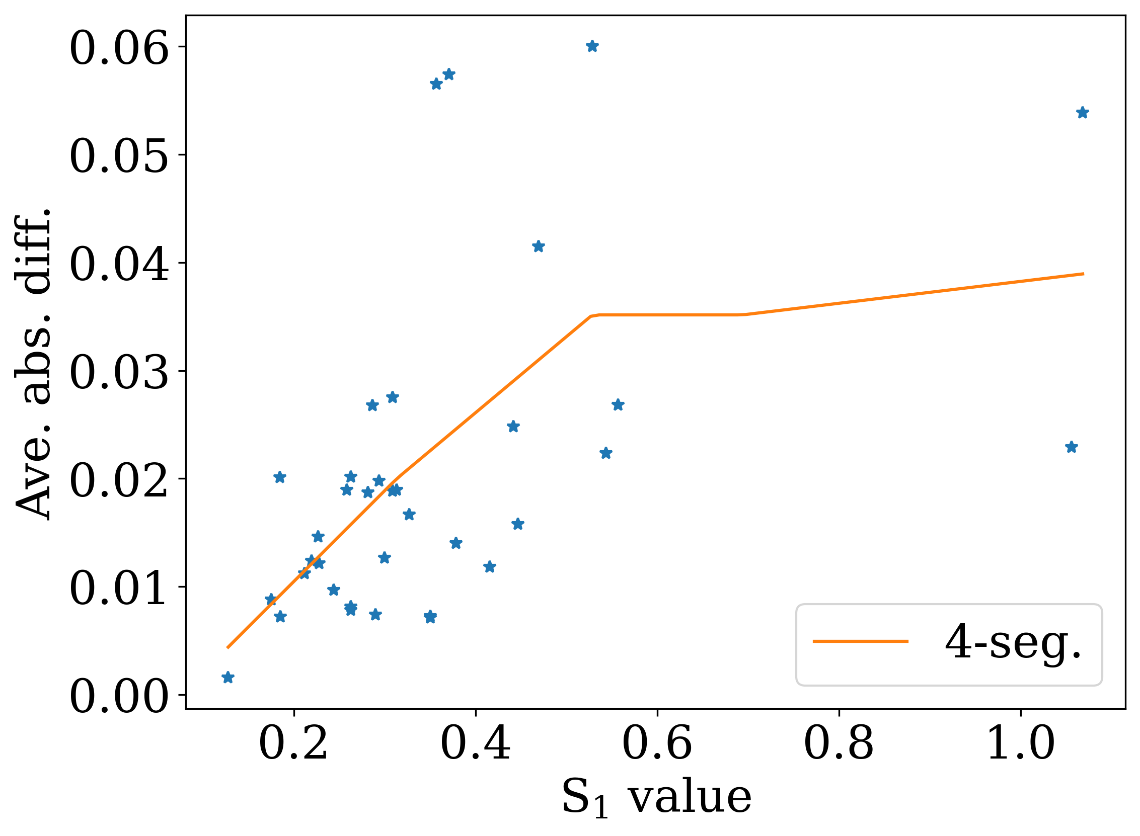
(a)

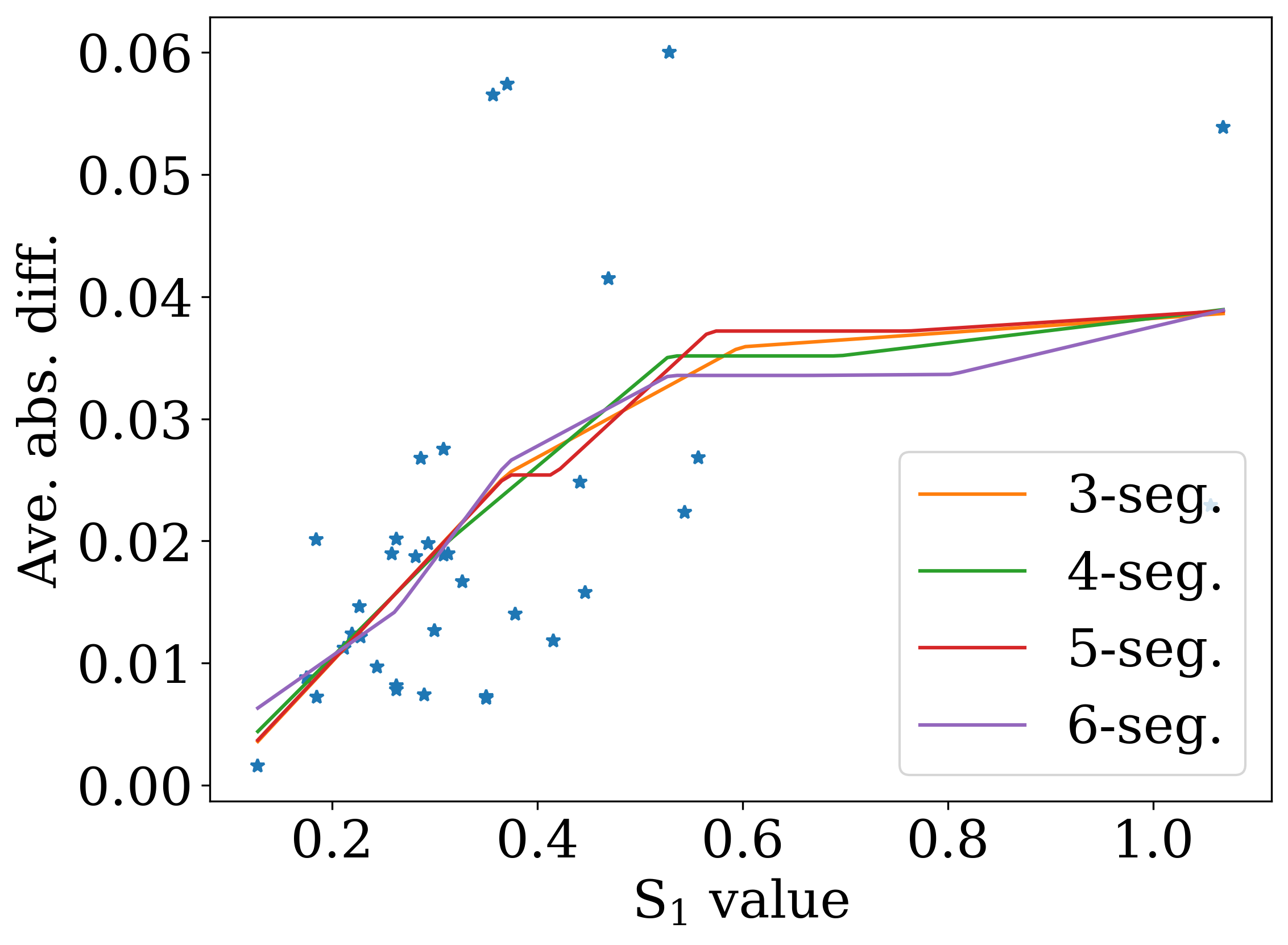
(b)

Figure 19: The averaged absolute error in geometry optimization as a function of the $S_{1}$ value. (19(a)) The orange line corresponds to a piecewise linear fit to the data using four segments for the piecewise linear function. (19(b)) Piecewise linear fits to the data with a varying number of segments.

6.1.2 S₂-diagnostic Correlations

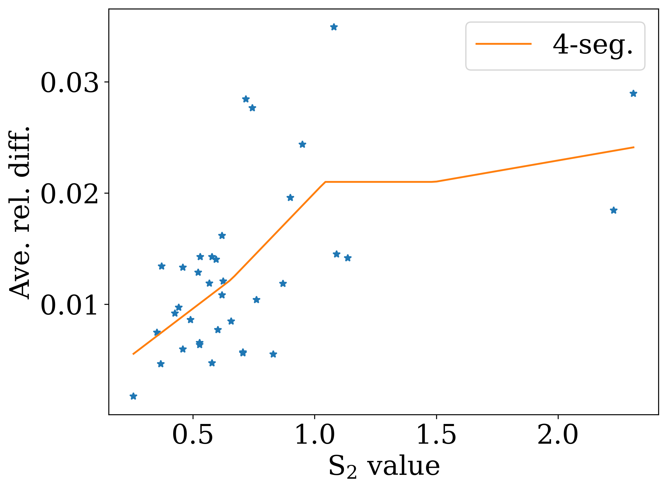
(a)

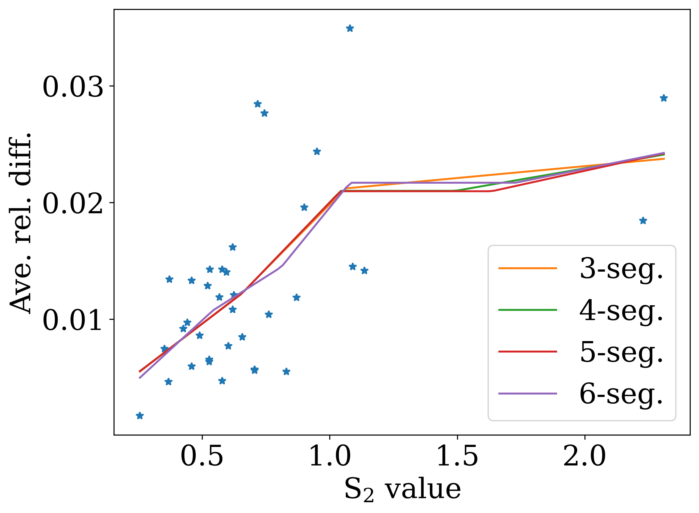
(b)

Figure 20: The averaged relative error in geometry optimization as a function of the $S_{2}$ value. (20(a)) The orange line corresponds to a piecewise linear fit to the data using four segments for the piecewise linear function. (20(b)) Piecewise linear fits to the data with a varying number of segments.

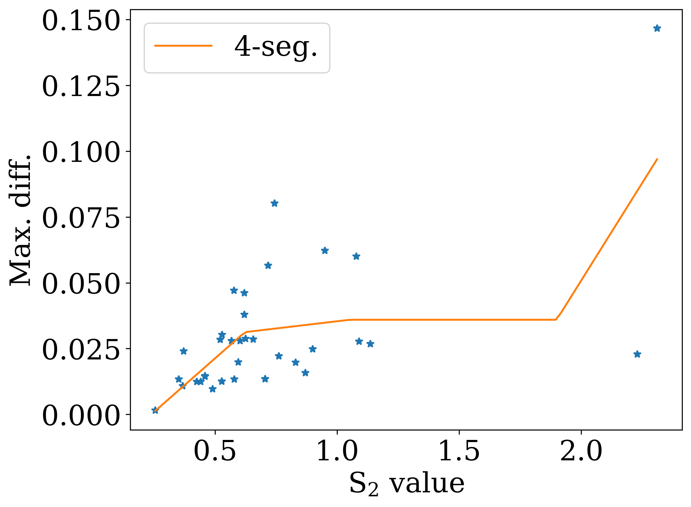
(a)

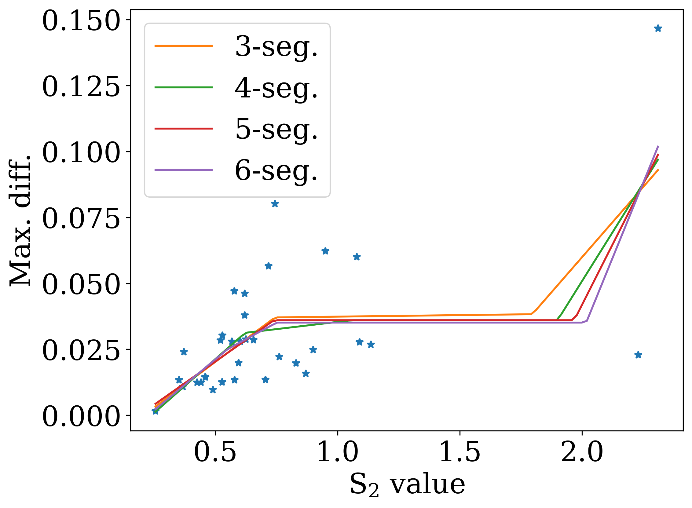
(b)

Figure 21: The maximal absolute error in geometry optimization as a function of the $S_{2}$ value. (21(a)) The orange line corresponds to a piecewise linear fit to the data using four segments for the piecewise linear function. (21(b)) Piecewise linear fits to the data with a varying number of segments.

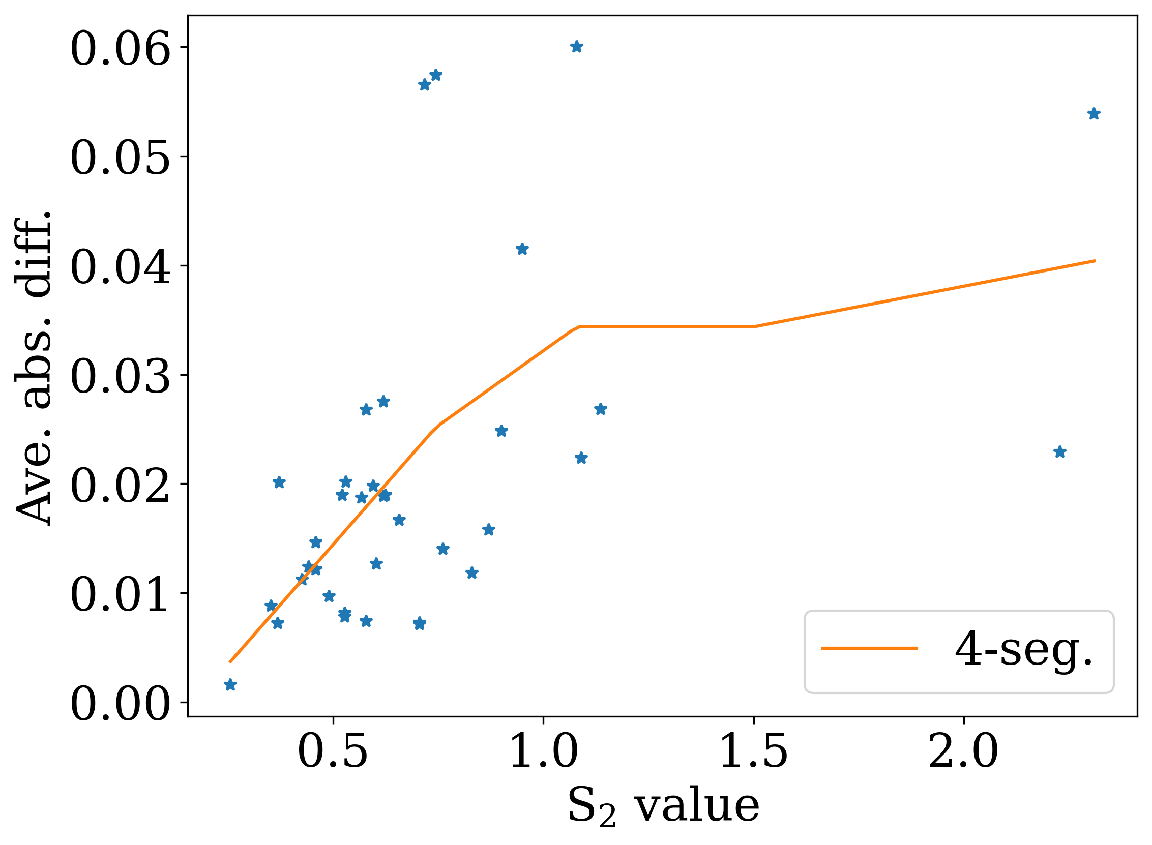
(a)

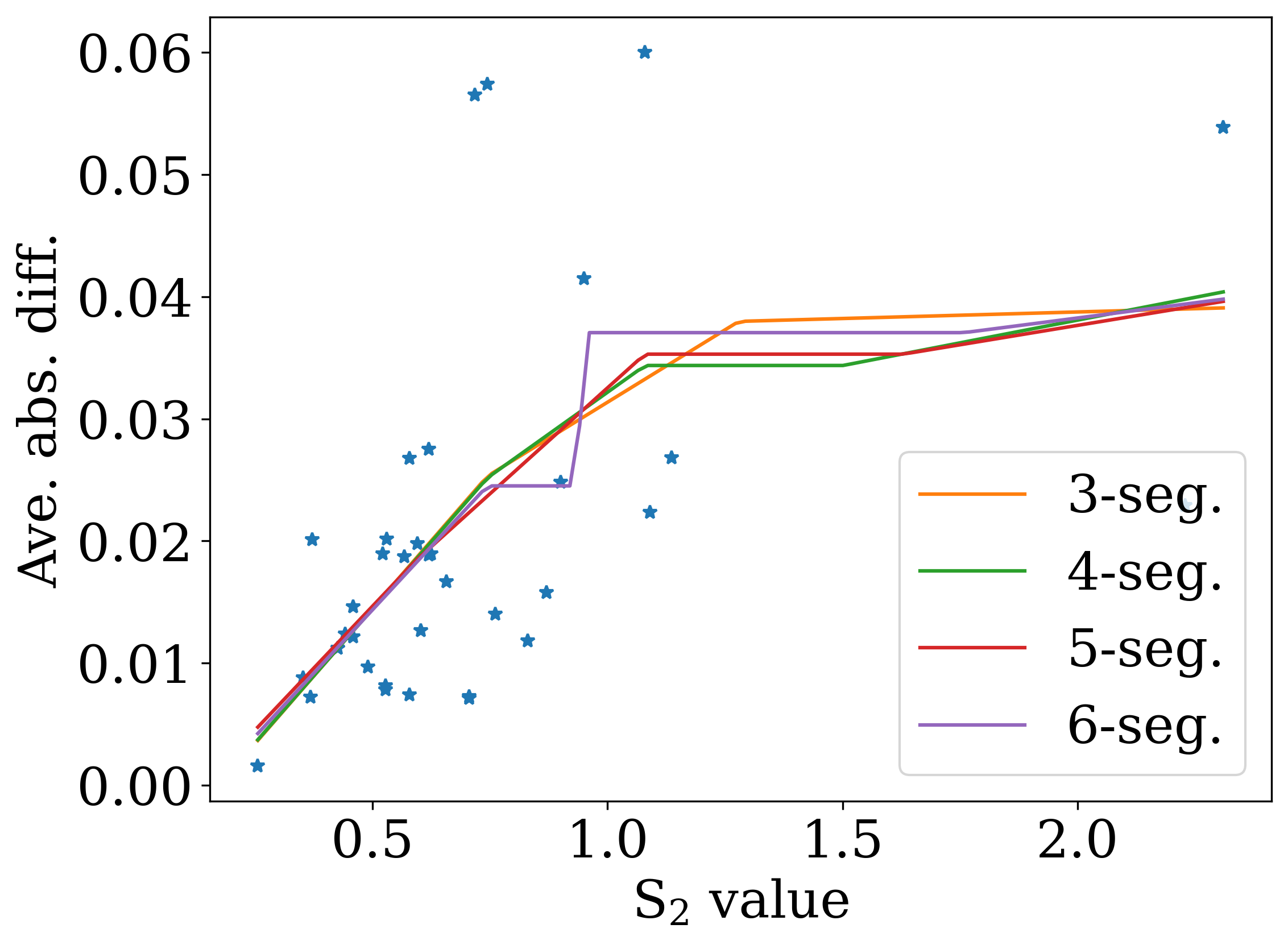
(b)

Figure 22: The averaged absolute error in geometry optimization as a function of the $S_{2}$ value. (22(a)) The orange line corresponds to a piecewise linear fit to the data using four segments for the piecewise linear function. (22(b)) Piecewise linear fits to the data with a varying number of segments.

6.1.3 S₂-diagnostic Correlations

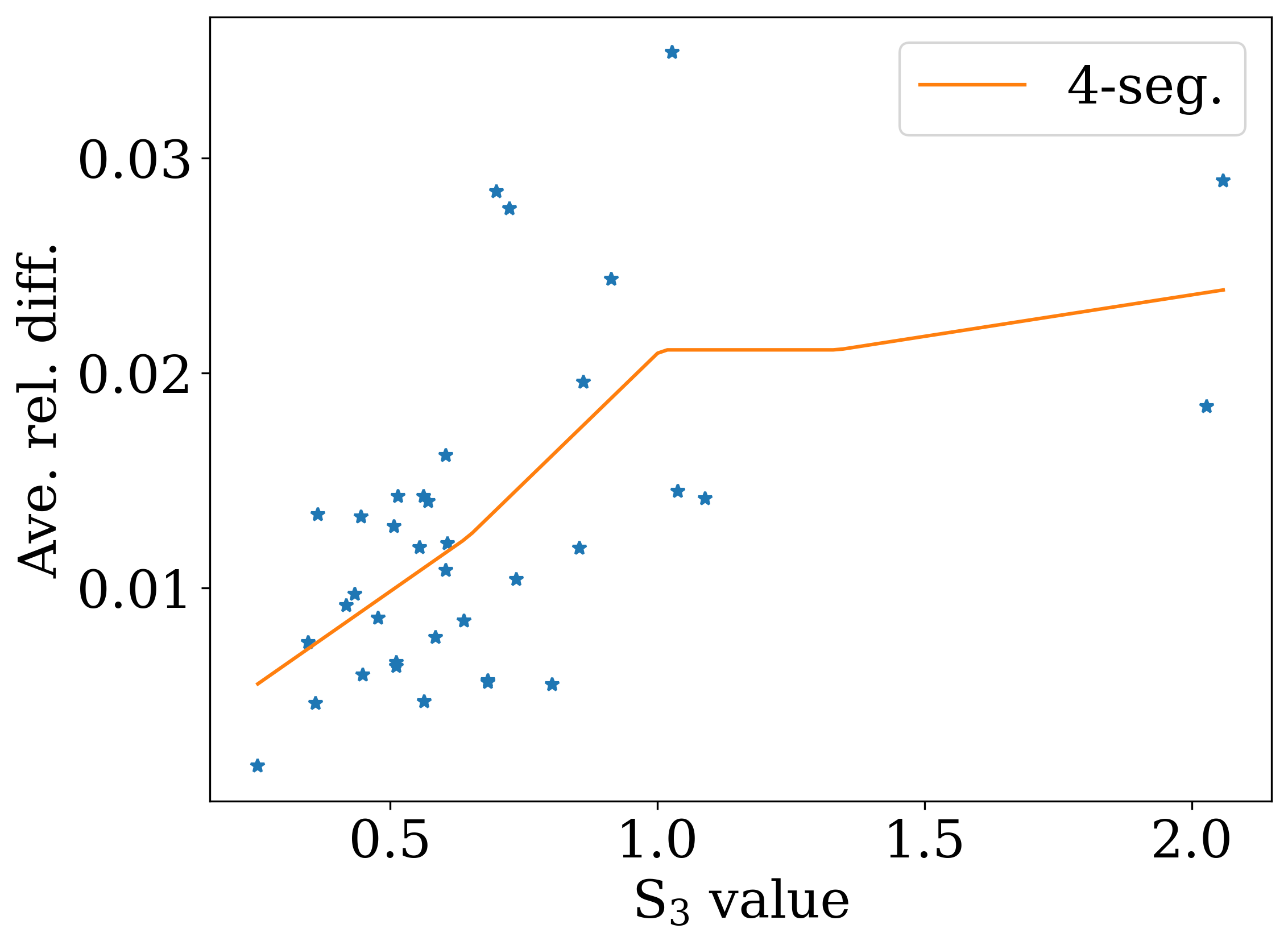
(a)

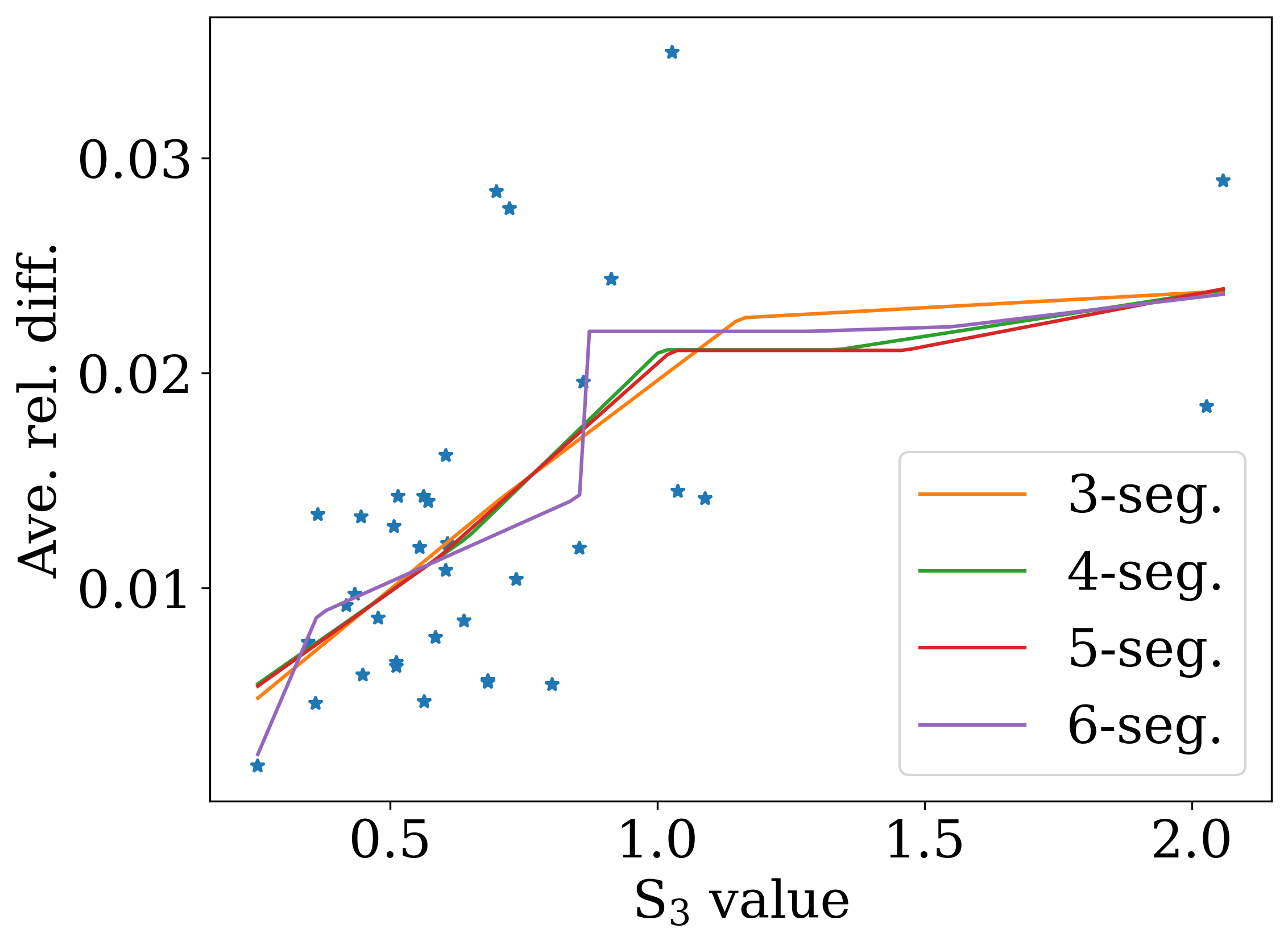
(b)

Figure 23: The averaged relative error in geometry optimization as a function of the $S_{3}$ value. (23(a)) The orange line corresponds to a piecewise linear fit to the data using four segments for the piecewise linear function. (23(b)) Piecewise linear fits to the data with a varying number of segments.

(a)

(b)

Figure 24: The maximal absolute error in geometry optimization as a function of the $S_{3}$ value. (24(a)) The orange line corresponds to a piecewise linear fit to the data using four segments for the piecewise linear function. (24(b)) Piecewise linear fits to the data with a varying number of segments.

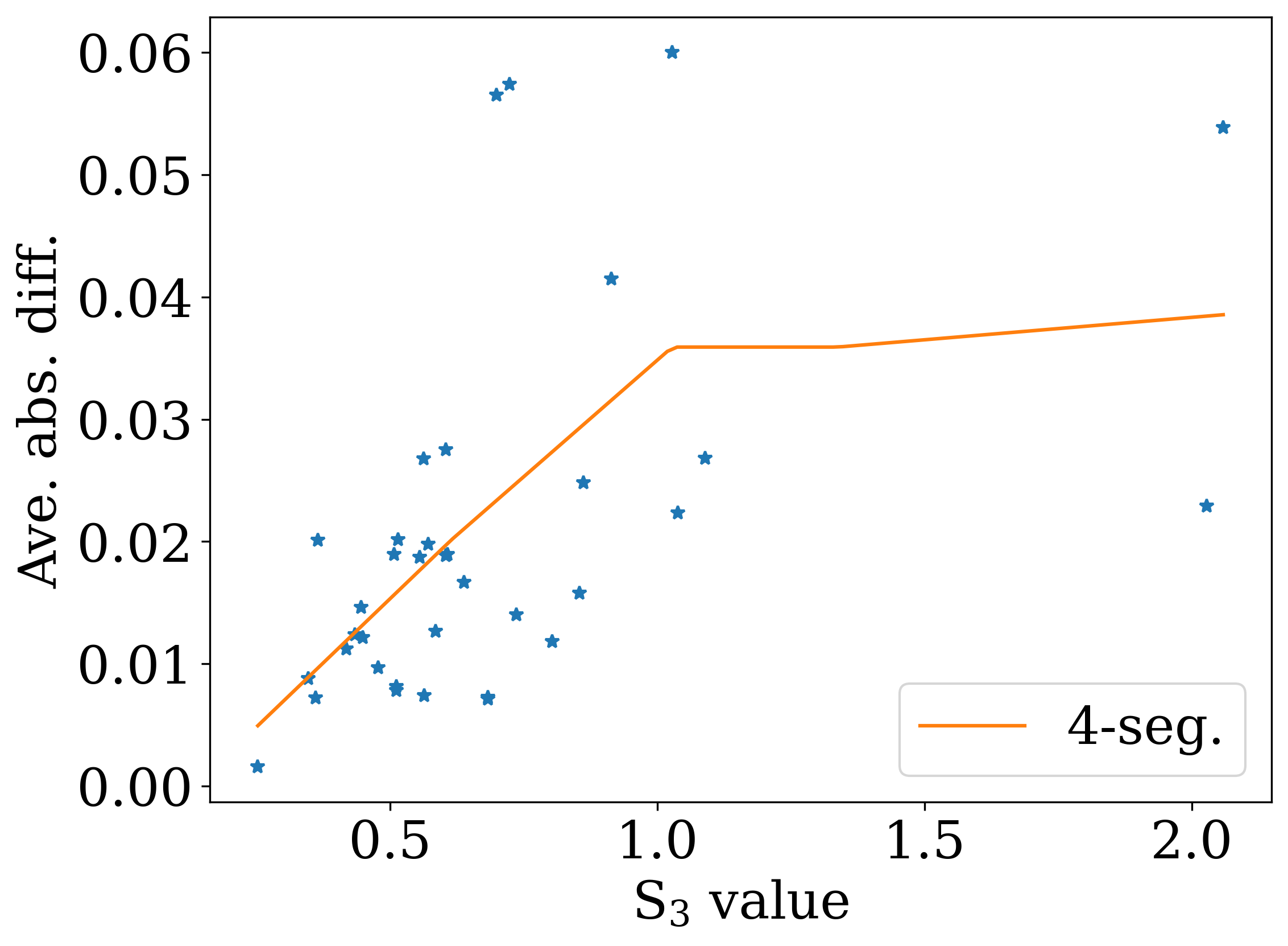
(a)

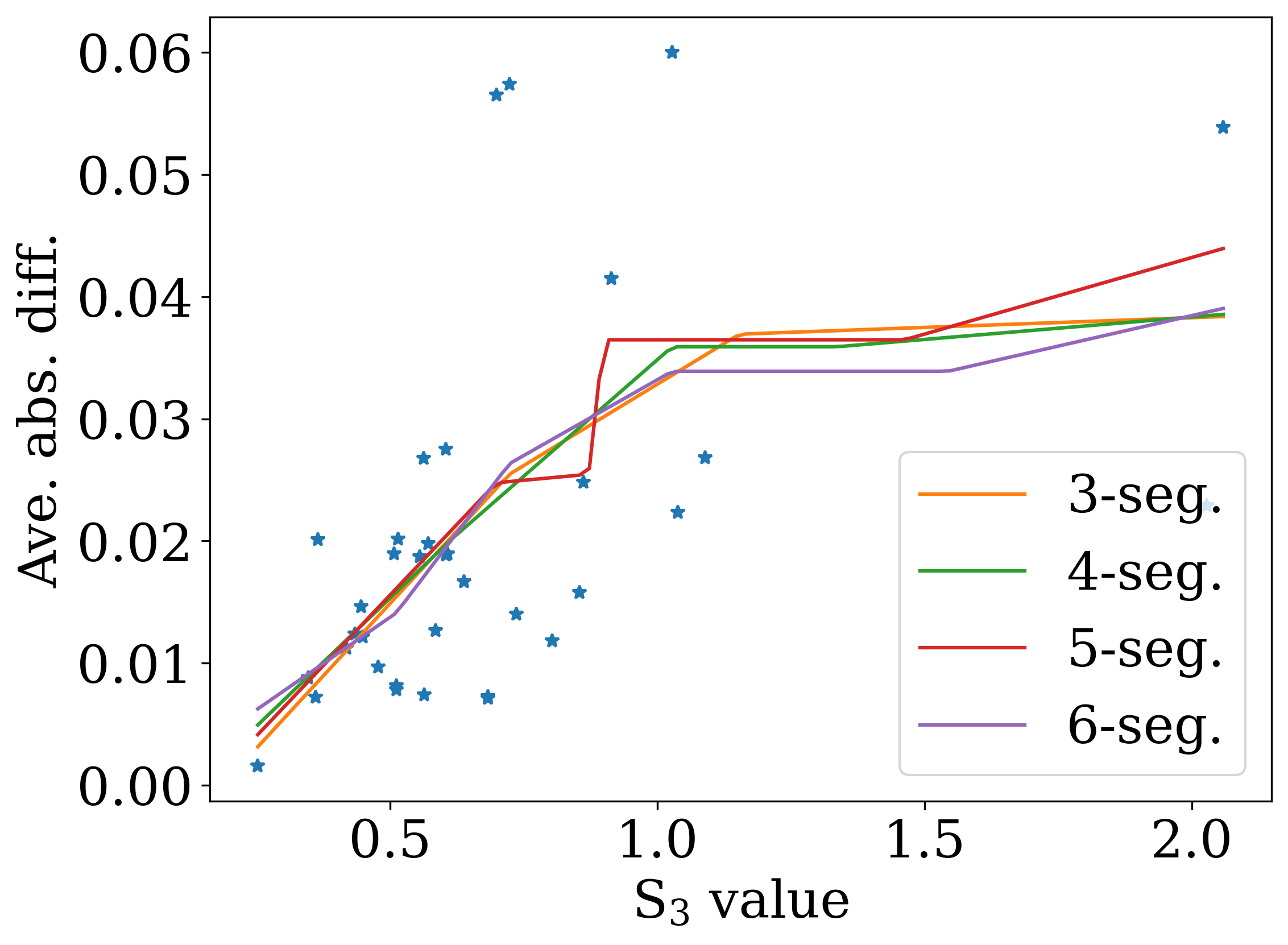
(b)

Figure 25: The averaged absolute error in geometry optimization as a function of the $S_{3}$ value. (25(a)) The orange line corresponds to a piecewise linear fit to the data using four segments for the piecewise linear function. (25(b)) Piecewise linear fits to the data with a varying number of segments.

6.2 Transition State Models

Here we shall compare the performance of the $S$-diagnostics and the previously used $T_{1}$, $D_{1}$, and $D_{2}$ diagnostics.

(a)

(a)

(a)

(a)

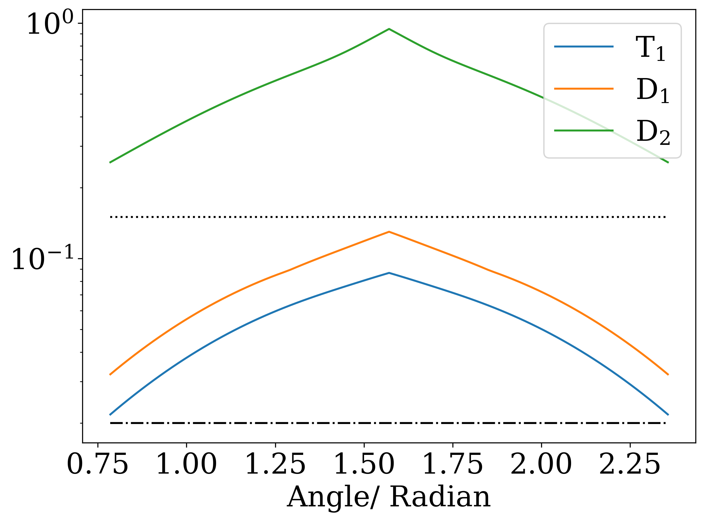
(b)

Figure 29: (29(a)) shows the $S$-diagnostics (29(b)) shows the previously suggested $T_{1}$, $D_{1}$ and $D_{2}$ diagnostics

References

- Bartlett and Musial 2007 Bartlett, R.; Musial, M. Coupled-cluster theory in quantum chemistry. Rev. Mod. Phys. 2007, 79, 291–352
- Raghavachari et al. 1989 Raghavachari, K.; Trucks, G. W.; Pople, J. A.; Head-Gordon, M. A fifth-order perturbation comparison of electron correlation theories. Chem. Phys. Lett. 1989, 157, 479–483
- Lee et al. 1989 Lee, T. J.; Rice, J. E.; Scuseria, G. E.; Schaefer, H. F. Theor. Chim. Acta 1989, 75, 81
- Lee and Taylor 1989 Lee, T. J.; Taylor, P. R. A diagnostic for determining the quality of single‐reference electron correlation methods. Int. J. Quantum Chem. 1989, 36, 199–207
- Janssen and Nielsen 1998 Janssen, C. L.; Nielsen, I. M. New diagnostics for coupled-cluster and Møller–Plesset perturbation theory. Chem. Phys. Lett. 1998, 290, 423 – 430
- Nielsen and Janssen 1999 Nielsen, I. M.; Janssen, C. L. Double-substitution-based diagnostics for coupled-cluster and Møller–Plesset perturbation theory. Chem. Phys. Lett. 1999, 310, 568 – 576
- Giner et al. 2018 Giner, E.; Tew, D. P.; Garniron, Y.; Alavi, A. Interplay between Electronic Correlation and Metal–Ligand Delocalization in the Spectroscopy of Transition Metal Compounds: Case Study on a Series of Planar Cu2+ Complexes. J. Chem. Theory Comput. 2018, 14, 6240–6252
- Bartlett et al. 2020 Bartlett, R. J.; Park, Y. C.; Bauman, N. P.; Melnichuk, A.; Ranasinghe, D.; Ravi, M.; Perera, A. Index of multi-determinantal and multi-reference character in coupled-cluster theory. J. Chem. Phys. 2020, 153, 234103
- Schneider 2009 Schneider, R. Analysis of the Projected Coupled Cluster Method in Electronic Structure Calculation. Numer. Math. 2009, 113, 433–471
- Helgaker and Jørgensen 1988 Helgaker, T.; Jørgensen, P. Analytical Calculation of Geometrical Derivatives in Molecular Electronic Structure Theory. Adv. Quant. Chem. 1988, 19, 183–245
- Kvaal 2022 Kvaal, S. Three Lagrangians for the complete-active space coupled-cluster method. arXiv preprint arXiv:2205.08792 2022,
- Arponen 1983 Arponen, J. S. Variational principles and linked-cluster exp S expansions for static and dynamic many-body problems. Ann. Phys. 1983, 151, 311–382
- Arponen et al. 1987 Arponen, J. S.; Bishop, R. F.; Pajanne, E. Extended coupled-cluster method. I. Generalized coherent bosonization as a mapping of quantum theory into classical Hamiltonian mechanics. Phys. Rev. A 1987, 36, 2519–2538
- Arponen et al. 1987 Arponen, J. S.; Bishop, R. F.; Pajanne, E. Extended coupled-cluster method. II. Excited states and generalized random-phase approximation. Phys. Rev. A 1987, 36, 2539–2549
- Laestadius and Kvaal 2018 Laestadius, A.; Kvaal, S. Analysis of the extended coupled-cluster method in quantum chemistry. SIAM J. Numer. Anal. 2018, 56, 660–683
- Faulstich and Oster 2022 Faulstich, F. M.; Oster, M. Coupled cluster theory: Towards an algebraic geometry formulation. arXiv:2211.10389 2022,
- Aubin 2011 Aubin, J.-P. Applied functional analysis; John Wiley & Sons, 2011
- Rohwedder 2013 Rohwedder, T. The Continuous Coupled Cluster Formulation for the Electronic Schrödinger Equation. ESAIM: Math. Modell. Numer. Anal. 2013, 47, 421–447
- Rohwedder and Schneider 2013 Rohwedder, T.; Schneider, R. Error Estimates for the Coupled Cluster Method. ESAIM: Math. Modell. Numer. Anal. 2013, 47, 1553–1582
- Laestadius and Faulstich 2019 Laestadius, A.; Faulstich, F. M. The coupled-cluster formalism -– a mathematical perspective. Mol. Phys. 2019, 117, 2362–2373
- S. Kvaal and Bodenstein 2020 S. Kvaal, A. L.; Bodenstein, T. Guaranteed convergence for a class of coupled-cluster methods based on Arponen’s extended theory. Mol. Phys. 2020,
- Beran and Head-Gordon 2004 Beran, G. J. O.; Head-Gordon, M. Extracting dominant pair correlations from many-body wave functions. J. Chem. Phys. 2004, 121, 78–88
- Sun et al. 2018 Sun, Q.; Berkelbach, T. C.; Blunt, N. S.; Booth, G. H.; Guo, S.; Li, Z.; Liu, J.; McClain, J. D.; Sayfutyarova, E. R.; Sharma, S., et al. PySCF: the Python-based simulations of chemistry framework. WIREs Comput. Mol. Sci. 2018, 8, e1340
- Sun et al. 2020 Sun, Q.; Zhang, X.; Banerjee, S.; Bao, P.; Barbry, M.; Blunt, N. S.; Bogdanov, N. A.; Booth, G. H.; Chen, J.; Cui, Z.-H., et al. Recent developments in the PySCF program package. J. Chem. Phys. 2020, 153, 024109
- Sun 2015 Sun, Q. Libcint: An efficient general integral library for g aussian basis functions. J. Comput. Chem. 2015, 36, 1664–1671
- Myers et al. 2013 Myers, J. L.; Well, A. D.; Lorch, R. F. Research design and statistical analysis; Routledge, 2013
- Hermann 2021 Hermann, J. PyBerny. 2021; https://github.com/jhrmnn/pyberny
- 28 Johnson, R. Computational Chemistry Comparison and Benchmark Database, NIST Standard Reference Database 101
- Purvis III et al. 1983 Purvis III, G. D.; Shepard, R.; Brown, F. B.; Bartlett, R. J. C2V Insertion pathway for BeH2: A test problem for the coupled-cluster single and double excitation model. Int. J. Quantum Chem. 1983, 23, 835–845
- Jankowski and Paldus 1980 Jankowski, K.; Paldus, J. Applicability of coupled-pair theories to quasidegenerate electronic states: A model study. Int. J. Quantum Chem. 1980, 18, 1243–1269
- Van Voorhis and Head-Gordon 2000 Van Voorhis, T.; Head-Gordon, M. Benchmark variational coupled cluster doubles results. The Journal of Chemical Physics 2000, 113, 8873–8879
- Bulik et al. 2015 Bulik, I. W.; Henderson, T. M.; Scuseria, G. E. Can single-reference coupled cluster theory describe static correlation? Journal of chemical theory and computation 2015, 11, 3171–3179
- Faulstich et al. 2019 Faulstich, F. M.; Laestadius, A.; Legeza, O.; Schneider, R.; Kvaal, S. Analysis of the tailored coupled-cluster method in quantum chemistry. SIAM J. Numer. Anal. 2019, 57, 2579–2607