Neural networks learn to magnify areas near decision boundaries

Abstract

In machine learning, there is a long history of trying to build neural networks that can learn from fewer example data by baking in strong geometric priors. However, it is not always clear a priori what geometric constraints are appropriate for a given task. Here, we consider the possibility that one can uncover useful geometric inductive biases by studying how training molds the Riemannian geometry induced by unconstrained neural network feature maps. We first show that at infinite width, neural networks with random parameters induce highly symmetric metrics on input space. This symmetry is broken by feature learning: networks trained to perform classification tasks learn to magnify local areas along decision boundaries. This holds in deep networks trained on high-dimensional image classification tasks, and even in self-supervised representation learning. These results begins to elucidate how training shapes the geometry induced by unconstrained neural network feature maps, laying the groundwork for an understanding of this richly nonlinear form of feature learning.

Keywords: Geometric deep learning, representation learning, self-supervised learning, Riemannian geometry, neural networks

1 Introduction

The physical and digital worlds possess rich geometric structure. If endowed with appropriate inductive biases, machine learning algorithms can leverage these regularities to learn efficiently. However, it is unclear how one should uncover the geometric inductive biases relevant for a particular task. The conventional approach to this problem is to hand-design algorithms to embed certain geometric priors (Bronstein et al., 2021), but little attention has been given to an alternative possibility: Can we uncover useful inductive biases by studying the geometry learned by existing deep neural network models, which are known to be highly performant (LeCun et al., 2015; Zhang et al., 2021; Radhakrishnan et al., 2022)? Previous works have explored some aspects of the geometry induced by neural networks with random parameters (Poole et al., 2016; Amari et al., 2019; Cho and Saul, 2009, 2011; Zavatone-Veth and Pehlevan, 2022; Hauser and Ray, 2017; Benfenati and Marta, 2023b), but we lack a rigorous understanding of data-dependent changes in representational geometry over training.

In this work, we aim to inaugurate a program of empirical research on the geometric structure of learned feature maps, with the eventual aim of gaining a deeper understanding of what geometric inductive biases are optimal in settings where one lacks significant prior intution. As a first step towards a deeper understanding of the geometry of trained deep network feature maps, we explore the possibility that neural networks learn to enhance local input disciminability over the course of training. Concretely, we formalize and test the following hypothesis:

Hypothesis 1

Deep neural networks trained to perform supervised classification tasks using standard gradient-based methods learn to magnify areas near decision boundaries.

This hypothesis is inspired by a series of influential papers published around the turn of the 21^st century by Amari and Wu. They proposed that the generalization performance of support vector machine (SVM) classifiers on small-scale tasks could be improved by transforming the kernel to expand the Riemannian volume element near decision boundaries (Amari and Wu, 1999; Wu and Amari, 2002; Williams et al., 2007). This proposal was based on the idea that this local magnification of areas improves class discriminability (Cho and Saul, 2011; Amari and Wu, 1999; Burges, 1999).

Our primary contributions are:

• In §4, we study general properties of the metric induced by shallow fully-connected neural networks. In §4.2, we compute the volume element and curvature of the metric induced by infinitely wide shallow networks with Gaussian weights and smooth activation functions, showing that it is spherically symmetric. These results provide a baseline for our tests of Hypothesis 1.

• In §6, we empirically show that training shallow networks on simple two-dimensional classification tasks expands the volume element along decision boundaries, consistent with Hypothesis 1. In §7.2 and 7.3, we provide evidence that deep residual networks trained on more complex image classification tasks (MNIST and CIFAR-10) behave similarly.

• Finally, in §7.4, we demonstrate how our approach can be applied to the self-supervised learning method Barlow Twins, showing how area expansion can emerge even without supervised training.

In total, our results provide a preliminary picture of how feature learning shapes the geometry induced by neural network feature maps. These observations open new avenues for investigating when this richly nonlinear form of feature learning is required for good generalization in deep networks.

2 Preliminaries

To allow us to formalize Hypothesis 1, we begin by introducing the basic idea of the Riemannian geometry of feature space representations. Our setup and notation largely follow Burges (1999), which in turn follows the conventions of Dodson and Poston (1991). We use the Einstein summation convention; summation over all repeated indices is implied.

2.1 Feature embeddings as Riemannian manifolds

Consider $d$-dimensional data living in some submanifold $\mathcal{D}\subseteq\mathbb{R}^{d}$. Let the feature map $\mathbf{\Phi}:\mathbb{R}^{d}\to\mathcal{H}$ be a map from $\mathbb{R}^{d}$ to some separable Hilbert space $\mathcal{H}$ of possibly infinite dimension $n$, with $\mathbf{\Phi}(\mathcal{D})=\mathcal{M}\subseteq\mathcal{H}$. We index input space dimensions by Greek letters $\mu,\nu,\rho,\ldots\in[d]$ and feature space dimensions by Latin letters $i,j,k,\ldots\in[n]$. Assume that $\mathbf{\Phi}$ is $\mathcal{C}^{\ell}$ for $\ell\geq 3$, and is everywhere of rank $r=\min\{d,n\}$. If $r=d$, then $\mathcal{M}$ is a $d$-dimensional $\mathcal{C}^{\ell}$ manifold immersed in $\mathcal{H}$. If $\ell=\infty$, then $\mathcal{M}$ is a smooth manifold. In contrast, if $r<d$, then $\mathcal{M}$ is a $d$-dimensional $\mathcal{C}^{\ell}$ manifold submersed in $\mathcal{H}$. The flat metric on $\mathcal{H}$ can then be pulled back to $\mathcal{M}$, with components

$$g_{\mu\nu}=\partial_{\mu}\Phi_{i}\partial_{\nu}\Phi_{i},$$ (1)

where we write $\partial_{\mu}\equiv\partial/\partial x^{\mu}$. If we define the feature kernel

$$k(\mathbf{x},\mathbf{y})=\Phi_{i}(\mathbf{x})\Phi_{i}(\mathbf{y})$$ (2)

for $\mathbf{x},\mathbf{y}\in\mathcal{D}$, then the resulting metric can be written in terms of the kernel as

$$g_{\mu\nu}=[\partial_{x_{\mu}}\partial_{y_{\nu}}k(\mathbf{x},\mathbf{y})]_{\mathbf{y}=\mathbf{x}}=(1/2)\partial_{x_{\mu}}\partial_{x_{\nu}}k(\mathbf{x},\mathbf{x})-[\partial_{y_{\mu}}\partial_{y_{\nu}}k(\mathbf{x},\mathbf{y})]_{\mathbf{y}=\mathbf{x}}.$$ (3)

This formula applies even if $n=\infty$, giving the metric induced by the feature embedding associated to a suitable Mercer kernel (Burges, 1999; Amari and Wu, 1999).

If $r=d$ and the pullback metric $g_{\mu\nu}$ is full rank, then $(\mathcal{M},g)$ is a $d$-dimensional Riemannian manifold (Dodson and Poston, 1991; Burges, 1999). However, if the pullback $g_{\mu\nu}$ is a degenerate metric, as must be the case if $r<d$, then $(\mathcal{M},g)$ is a singular semi-Riemannian manifold (Benfenati and Marta, 2023b; Kupeli, 2013). In this case, if we let $\sim$ be the equivalence relation defined by identifying points with vanishing pseudodistance, the quotient $(\mathcal{M}/\sim,g)$ is a Riemannian manifold (Benfenati and Marta, 2023b). Unless noted otherwise, our results will focus on the non-singular case. We denote the matrix inverse of the metric tensor by $g^{\mu\nu}$, and we raise and lower input space indices using the metric.

2.2 Volume element and curvature

With this setup, $(\mathcal{M},g)$ is a Riemannian manifold; hence, we have at our disposal a powerful toolkit with which we may study its geometry. We will focus on two geometric properties of $(\mathcal{M},g)$. First, the volume element is given by

$$dV=\sqrt{\det g}\,d^{d}x,$$ (4)

where the factor $\sqrt{\det g}$ measures how local areas in input space are magnified by the feature map (Dodson and Poston, 1991; Amari and Wu, 1999; Burges, 1999). It is this measure of volume which we will use in testing Hypothesis 1. Second, we consider the intrinsic curvature of the manifold, which is characterized by the Riemann tensor $R^{\mu}_{\nu\alpha\beta}$ (Dodson and Poston, 1991). If $R^{\mu}_{\nu\alpha\beta}=0$, then the manifold is intrinsically flat. As a tractable measure, we focus on the Ricci curvature scalar $R=g^{\beta\nu}R^{\alpha}_{\nu\alpha\beta}$, which measures the deviation of the volume of an infinitesimal geodesic ball in the manifold from that in flat space (Dodson and Poston, 1991). In the singular case, we can compute the volume element on $\mathcal{M}/\sim$ at a given point by taking the square root of the product of the non-zero eigenvalues of the degenerate metric $g_{\mu\nu}$ at that point (Benfenati and Marta, 2023b). However, the curvature in this case is generally not straightforward to compute; we will therefore leave this issue for future work. Indeed, we will mostly focus on the volume element—as presaged by Hypothesis 1—due to computational constraints, which we discuss further in §7.2 and in Appendix G.

2.3 Shallow neural network feature maps

In this work, we consider feature maps given by the hidden layer representations of neural networks (Williams, 1997; Neal, 1996; LeCun et al., 2015; Cho and Saul, 2009, 2011; Lee et al., 2018; Matthews et al., 2018; Hauser and Ray, 2017; Benfenati and Marta, 2023b). In our theoretical investigations, we focus on shallow fully-connected neural networks, which have feature maps of the form

$$\Phi_{j}(\mathbf{x})=\frac{1}{\sqrt{n}}\phi(\mathbf{w}_{j}\cdot\mathbf{x}+b_{j})$$ (5)

for weights $\mathbf{w}_{j}$, biases $b_{j}$, and an activation function $\phi$, where we abbreviate $\mathbf{w}\cdot\mathbf{x}=w_{\mu}x_{\mu}$. In this case, the feature space dimension $n$ is equal to the number of hidden units, i.e., the width of the hidden layer. We scale the components of the feature map by $n^{-1/2}$ such that the associated kernel $k(\mathbf{x},\mathbf{y})=\Phi_{i}(\mathbf{x})\Phi_{i}(\mathbf{y})$ and metric have the form of averages over hidden units, and therefore should be well-behaved at large widths (Neal, 1996; Williams, 1997). We will assume that $\phi$ is $\mathcal{C}^{k}$ for $k\geq 3$, so that this feature map satisfies the smoothness conditions required in the setup above. We will also assume that the activation function and weight vectors are such that the Jacobian $\partial_{\mu}\Phi_{j}$ is full-rank, i.e., is of rank $\min\{d,n\}$. Then, the shallow network feature map satisfies the required conditions for the feature embedding to be a (possibly singular) Riemannian manifold. These conditions extend directly to deep fully-connected networks formed by composing shallow feature maps (Hauser and Ray, 2017; Benfenati and Marta, 2023b).

3 Related works

Having established the geometric preliminaries of §2, we can give a more complete overview of related works. First, in the standard program of geometric deep learning with smooth manifolds, one seeks to define a feature map that induces a tractable metric on the input space Bronstein et al. (2021). Of particular interest are manifolds with constant negative or positive curvature—hyperbolic and spherical spaces, respectively—which have enjoyed ample success in multiple machine learning tasks. To give just a few examples, hyperbolic representations have demonstrated performance gains relative to unconstrained representations in textual entailment (Nickel and Kiela, 2017), image classification (Khrulkov et al., 2020), knowledge graph embedding (Chami et al., 2020), single-cell clustering (Klimovskaia et al., 2020), et cetera. Their positively-curved spherical counterparts provide competitive performance in tasks including 3D recognition (Cohen et al., 2018), shape detection (Esteves et al., 2018), token embeddings (Meng et al., 2019), and many others. Importantly, these successes were enabled by prior knowledge of which geometries are optimal for a given set of data. For instance, the use of hyperbolic representations for graph embedding is motivated by the fact that tree graphs embed in low-dimensional hyperbolic space with low distortion (Gupta, 1999; Sarkar, 2011). Some effort has been devoted to moving beyond the simple constant-curvature setting by considering products of fixed-curvature manifolds (Gu et al., 2018; Skopek et al., 2020), but when a variable-curvature representation is optimal for generalization is as yet poorly understood. Our goal in this work is to move towards the investigation of such settings, and to those where one cannot leverage prior information about the geometric structure of the data at hand.

As introduced above, our hypothesis for how the Riemannian geometry of neural network representations changes during training is directly inspired by the work of Amari and Wu (1999). In a series of works (Amari and Wu, 1999; Wu and Amari, 2002; Williams et al., 2007), they proposed to modify the kernel of a support vector machine as

$$\tilde{k}(\mathbf{x},\mathbf{y})=h(\mathbf{x})h(\mathbf{y})k(\mathbf{x},\mathbf{y})$$ (6)

for some positive scalar function $h(\mathbf{x})$ chosen such that the magnification factor $\sqrt{\det g}$ is large near the SVM’s decision boundary. Concretely, they proposed to fit an SVM with some base kernel $k$, choose

$$h(\mathbf{x})=\sum_{\mathbf{v}\in\textrm{SV}(k)}\exp\left[-\frac{\|\mathbf{x}-\mathbf{v}\|^{2}}{2\tau^{2}}\right]$$ (7)

for $\tau$ a bandwidth parameter and $\textrm{SV}(k)$ the set of support vectors for $k$, and then fit an SVM with the modified kernel $\tilde{k}$. Here, $\|\cdot\|$ denotes the Euclidean norm. This process could then be iterated, yielding a sequence of modified kernels. As we review in Appendix F, this update expands the volume element near support vectors—and thus near SVM decision boundaries—for an appropriate range of the bandwidth parameters. This hand-designed form of iterative feature learning could improve generalization performance on a set of small-scale tasks (Amari and Wu, 1999; Wu and Amari, 2002; Williams et al., 2007).

The geometry induced by common kernels was investigated by Burges (1999), who established a broad range of technical results. He showed that any translation-invariant kernel of the form $k(\mathbf{x},\mathbf{y})=k(\|\mathbf{x}-\mathbf{y}\|^{2})$—not just the radial basis function—-yields a flat, constant metric, and gave a detailed characterization of polynomial kernels $k(\mathbf{x},\mathbf{y})=(\mathbf{x}\cdot\mathbf{y})^{q}$. Cho and Saul (2011) subsequently analyzed the geometry induced by arc-cosine kernels, i.e., the feature kernels of infinitely-wide shallow neural networks with threshold-power law activation functions $\phi(x)=\max\{0,x\}^{q}$ and random parameters (Cho and Saul, 2009). Our results on infinitely-wide networks for general smooth activation functions build on these works. More recent works have studied the representational geometry of deep networks with random Gaussian parameters in the limit of large width and depth (Poole et al., 2016; Amari et al., 2019), tying into a broader line of research on infinite-width limits in which inference and prediction is captured by a kernel machine (Neal, 1996; Williams, 1997; Daniely et al., 2016; Lee et al., 2018; Matthews et al., 2018; Yang, 2019; Yang and Hu, 2021; Zavatone-Veth et al., 2021; Zavatone-Veth and Pehlevan, 2022; Bordelon and Pehlevan, 2022). Our results on the representational geometry of wide shallow networks with smooth activation functions build on these ideas, particularly those relating activation function derivatives to input discriminability (Poole et al., 2016; Daniely et al., 2016; Zavatone-Veth and Pehlevan, 2021, 2022).

Particularly closely related to our work are several recent papers that aim to study the curvature of neural network representations. Hauser and Ray (2017); Benfenati and Marta (2023b) discuss formal principles of Riemannian geometry in deep neural networks, but do not characterize how training shapes the geometry. Kaul and Lall (2020) aimed to study the curvature of metrics induced by the outputs of pretrained classifiers. However, their work is limited by the fact that they estimate input-space derivatives using inexact finite differences under the strong assumption that the input data is confined to a known smooth submanifold of $\mathbb{R}^{d}$. In very recent work, Benfenati and Marta (2023a) have used the geometry induced by the full input-output mapping to reconstruct iso-response curves of deep networks. The metric induced on input space by the Fisher information metric on classifier outputs was also considered by Nayebi and Ganguli (2017), who showed that this metric magnifies areas near decision boundaries. For points to be classified correctly, this is in some sense necessarily true. Tron et al. (2022) built upon the idea of pulling from Fisher information metric to derive geodesically-aware adversarial attacks. In contrast to these works, our work focuses on hidden representations, and seeks to characterize the representational manifolds themselves. Finally, several recent works have studied the Riemannian geometry of the latent representations of deep generative models (Shao et al., 2018; Kuhnel et al., 2018; Wang and Ponce, 2021).

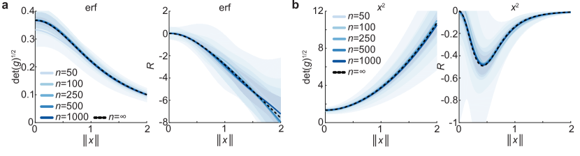
Figure 1: Convergence of geometric quantities for finite-width networks with Gaussian random parameters to the infinite-width limit. a. The magnification factor $\sqrt{\det g}$ (left) and Ricci scalar $R$ (right) as functions of the input norm $\|\mathbf{x}\|$ for networks with $\phi(x)=\operatorname{erf}(x/\sqrt{2})$. Empirical results for finite networks, computed using (9) and (B.15) are shown in blue, with solid lines showing the mean and shaded patches the standard deviation over 25 realizations of random Gaussian parameters. In all cases, $\sigma=\zeta=1$. The infinite-width result is shown as a black dashed line. b. As in a, but for normalized quadratic activation functions $\phi(x)=x^{2}/\sqrt{3}$.

4 Representational geometry of shallow neural network feature maps

4.1 Finite-width networks

We begin by studying general properties of the metrics induced by shallow neural networks. We first consider finite-width networks with fixed weights, assuming that $n\geq d$. Writing $z_{j}=\mathbf{w}_{j}\cdot\mathbf{x}+b_{j}$ for the preactivation of the $j$-th hidden unit, the general formula (1) for the metric yields

$$g_{\mu\nu}=\frac{1}{n}\phi^{\prime}(z_{j})^{2}w_{j\mu}w_{j\nu}.$$ (8)

This metric has the useful property that $\partial_{\alpha}g_{\mu\nu}$ is symmetric under permutation of its indices, hence the formula for the Riemann tensor simplifies substantially (Appendix A). We show in Appendix B that the determinant of the metric can be expanded as a sum over $d$-tuples of hidden units:

$$\det g=\frac{1}{n^{d}d!}M_{j_{1}\cdots j_{d}}^{2}\phi^{\prime}(z_{j_{1}})^{2}\cdots\phi^{\prime}(z_{j_{d}})^{2},$$ (9)

where $M_{j_{1}\cdots j_{d}}=\det([w_{j_{i}i}]_{1\leq i\leq d})$ is the minor of the weight matrix obtained by selecting units $j_{1},\ldots,j_{d}$.

We can also derive similar expansions for the Riemann tensor and Ricci scalar. The resulting expressions are rather unwieldy and not particularly illuminating, so we give their general forms only in Appendix B.3. However, in two dimensions the situation simplifies, as the Riemann tensor is completely determined by the Ricci scalar (Dodson and Poston, 1991; Misner et al., 2017) (Appendix B.1). In this case, we have the compact expression

$$(\det g)^{2}R =-\frac{3}{n^{3}}M_{jk}^{2}M_{ij}M_{ik}\phi^{\prime}(z_{i})^{2}\phi^{\prime}(z_{j})\phi^{\prime}(z_{k})\phi^{\prime\prime}(z_{j})\phi^{\prime\prime}(z_{k}).$$ (10)

This shows that in $d=2$ the curvature acquires contributions from each triple of distinct hidden units, hence if $n=2$ we have $R=0$. This follows from the fact that the feature map is in this case a change of coordinates on the two-dimensional manifold (Dodson and Poston, 1991).

A tractable example activation function for which these expressions can be usefully simplified is the error function $\phi(x)=\operatorname{erf}(x/\sqrt{2})$. In this case, the volume element and curvature expand as superpositions of Gaussian bumps. One can explicitly work out the center and scale of these bumps in terms of the network parameters, but the general result is not particularly illuminating, hence we defer it to Appendix B.4. This is reminiscent of Amari and Wu’s approach, which yields a Gaussian contribution to $\sqrt{\det g}$ from each support vector (see §3 and Appendix F). We illustrate this behavior in a worked toy example in Appendix B.4.

4.2 Geometry of infinite shallow networks

We now characterize the metric induced by infinite-width networks ($n\to\infty$) with Gaussian weights and biases

$$\mathbf{w}_{j}\sim_{\textrm{i.i.d.}}\mathcal{N}(\mathbf{0},\sigma^{2}\mathbf{I}_{d}),\quad b_{j}\sim_{\textrm{i.i.d.}}\mathcal{N}(0,\zeta^{2}),$$ (11)

as commonly chosen at initialization (LeCun et al., 2015; Lee et al., 2018; Matthews et al., 2018; Yang, 2019; Yang and Hu, 2021; Poole et al., 2016). For such networks, the hidden layer representation is described by the neural network Gaussian process (NNGP) kernel (Neal, 1996; Williams, 1997; Matthews et al., 2018; Lee et al., 2018):

$$k(\mathbf{x},\mathbf{y})=\lim_{n\to\infty}\frac{1}{n}\bm{\Phi}(\mathbf{x})\cdot\bm{\Phi}(\mathbf{y})=\mathbb{E}_{\mathbf{w},b}[\phi(\mathbf{w}\cdot\mathbf{x}+b)\phi(\mathbf{w}\cdot\mathbf{y}+b)]$$ (12)

For networks in the lazy regime, this kernel completely describes the representation after training (Yang and Hu, 2021; Bordelon and Pehlevan, 2022). In Appendix C, we show that the metric associated with the NNGP kernel can be written as

$$g_{\mu\nu}=e^{\Omega(\|\mathbf{x}\|^{2})}[\delta_{\mu\nu}+2\Omega^{\prime}(\|\mathbf{x}\|^{2})x_{\mu}x_{\nu}],$$ (13)

where the function $\Omega(\|\mathbf{x}\|^{2})$ is defined via $e^{\Omega(\|\mathbf{x}\|^{2})}=\sigma^{2}\mathbb{E}[\phi^{\prime}(z)^{2}]$ for $z\sim\mathcal{N}(0,\sigma^{2}\|\mathbf{x}\|^{2}+\zeta^{2})$. Therefore, like the metrics induced by other dot-product kernels, the NNGP metric has the form of a projection (Burges, 1999). Such metrics have determinant

$$\det g=e^{\Omega d}(1+2\|\mathbf{x}\|^{2}\Omega^{\prime})$$ (14)

and Ricci scalar

$$R =-\frac{3(d-1)e^{-\Omega}(\Omega^{\prime})^{2}\|\mathbf{x}\|^{2}}{(1+2\|\mathbf{x}\|^{2}\Omega^{\prime})^{2}}\left[d+2+2\|\mathbf{x}\|^{2}\left((d-2)\Omega^{\prime}+2\frac{\Omega^{\prime\prime}}{\Omega^{\prime}}\right)\right].$$ (15)

Thus, all geometric quantities are spherically symmetric, depending only on $\|\mathbf{x}\|^{2}$. Thanks to the assumption of independent Gaussian weights, the geometric quantities associated to the shallow Neural Tangent Kernel and to the deep NNGP will share this spherical symmetry (Appendix D) (Lee et al., 2018; Matthews et al., 2018; Yang, 2019; Yang and Hu, 2021). This generalizes the results of Cho and Saul (2011) for threshold-power law functions to arbitrary smooth activation functions. The relation between Gaussian norms of $\phi^{\prime}$ and input discriminability indicated by this result is consistent with previous studies (Poole et al., 2016; Daniely et al., 2016; Zavatone-Veth and Pehlevan, 2021, 2022). In short, unless the task depends only on the input norm, the geometry of infinite-width networks will not be linked to the task structure.

In Appendix C.2, we evaluate the geometric quantities of the NNGP for certain analytically tractable activation functions. The resulting expressions for $\sqrt{\det g}$ and $R$ are rather lengthy and not in of themselves particularly illuminating, so we discuss only their qualitative behavior here. For the error function $\phi(x)=\operatorname{erf}(x/\sqrt{2})$, $R$ is negative for all $d>1$, and both $R$ and $\sqrt{\det g}$ are monotonically decreasing functions of $\|\mathbf{x}\|$ for all $\zeta$ and $\sigma$. For monomials $\phi(x)\propto x^{q}$ for integer $q>1$, $\sqrt{\det g}$ is a monotonically increasing function of $\|\mathbf{x}\|^{2}$, while $R$ is again non-positive. However, in this case the behavior of $R$ depends on whether or not bias terms are present: if $\zeta=0$, then $R$ is a non-decreasing function of $\|\mathbf{x}\|^{2}$ that diverges towards $-\infty$ as $\|\mathbf{x}\|^{2}\downarrow 0$, while if $\zeta>0$, $R$ may be non-monotonic in $\|\mathbf{x}\|^{2}$. In Figure 1, we illustrate this behavior, and show convergence of the empirical geometry of finite networks with random Gaussian parameters to the infinite-width results. It is interesting to note that in both cases the curvature of the induced metric is negative; this geometric inductive bias of infinitely-wide neural networks could be interesting to investigate further in future work.

5 Changes in shallow network geometry under Bayesian inference at large but finite width

We now consider how the geometry of the pullback metric changes during training in networks that learn features, that is, outside of the lazy/kernel regime. Changes in the volume element and curvature during gradient descent training are challenging to study analytically, because feature-learning networks with solvable dynamics—deep linear networks (Saxe et al., 2013)—trivially yield flat, constant metrics. One could attempt to solve for the metric’s dynamics through time in infinite-width networks parameterized such that they learn features (Yang and Hu, 2021; Bordelon and Pehlevan, 2022), but we will not do so here.

We can make slightly more analytical progress for Bayesian neural networks at large but finite width. This setting is convenient because there is a fixed parameter posterior; one does not need to solve kernel or metric dynamics through time (Bordelon and Pehlevan, 2022). Moreover, if we are close to the Gaussian process limit—such that the feature kernel changes only infinitesimally—we can treat the effect of learning on the induced geometry perturbatively. In particular, we can leverage recent results on perturbative feature-learning corrections to the NNGP kernel in wide but finite networks (Zavatone-Veth et al., 2021; Roberts et al., 2022). As it is closer to the primary objective of the present paper, we will focus on corrections to the volume element. One could in principle compute perturbative corrections to the Riemann tensor and Ricci scalar, but we will not attempt that somewhat tedious mechanical exercise here (Misner et al., 2017).

In Appendix E, we use this approach to compute corrections to the volume element. In general, it is not possible to evaluate these corrections in closed form, and even when they can be evaluated they are not always particularly illuminating (Zavatone-Veth et al., 2021). However, one case in which we can make useful progress is when we constrain a network with monomial activation functions, no bias terms, and linear readout to interpolate a single training example $(\mathbf{x}_{a},\mathbf{y}_{a})$. Then, we can evaluate all required expectations analytically, and show that correction to $\langle\sqrt{\det g}\rangle$ is maximal for test points $\mathbf{x}$ such that $\mathbf{x}\parallel\mathbf{x}_{a}$, and minimal for $\mathbf{x}\perp\mathbf{x}_{a}$ (E.38). Here, we write $\langle\cdot\rangle$ for expectation with respect to the corresponding Bayes posterior. The sign of the correction is positive or negative depending on whether the second moment of the prior predictive is greater than or less than the norm of the output, respectively. In particular, the simplest such network has a normalized quadratic activation function $\phi(x)\propto x^{2}$, which yields

$$\frac{\langle\sqrt{\det g}\rangle}{\sqrt{\det\bar{g}}} =1+\frac{1}{n}\left(\frac{y_{a}^{2}}{\|\mathbf{x}_{a}\|^{4}}-1\right)\left(\frac{4}{3}\rho^{4}+(d+2)\rho^{2}+1\right)+\mathcal{O}\left(\frac{1}{n^{2}}\right),$$ (16)

where $\rho=\mathbf{x}_{a}\cdot\mathbf{x}/(\|\mathbf{x}_{a}\|\|\mathbf{x}\|)$ is the cosine of the angle between the training and test points, and $\bar{g}$ is the metric induced by the corresponding NNGP, which in this case has determinant proportional to the norm of the test point, $\sqrt{\det\bar{g}}\propto\|\mathbf{x}\|^{d}$. For example, if we train on a single point from the XOR task, $(1,1)\mapsto 0$, $\sqrt{\det g}$ will be contracted maximally along $x_{1}=x_{2}$. This simple case gives some intuition for how interpolating a single point shapes the network’s global representational geometry, showing that the training point’s influence is maximal for points parallel to it. Yet, the settings we can address are far removed from realistic network architectures and datasets.

6 Changes in shallow network geometry during gradient descent training

6.1 Changes in representational geometry for networks trained on two-dimensional toy tasks

Giiven the intractability of studying changes in geometry analytically, we resort to numerical experiments. For details of our numerical methods, see Appendix G. To build intuition, we first consider networks trained on simple two-dimensional tasks, for which we can directly visualize the input space. We first consider a toy binary classification task with sinusoidal boundary, inspired by the task considered in the original work of Amari and Wu (1999). We train networks with sigmoidal activation functions of varying widths to perform this task, and visualize the resulting geometry over the course of training in Figures 2. At initialization, the peaks in the volume element lack a clear relation to the structure of the task, with approximate rotational symmetry at large widths as we would expect from §4.2. As the network’s decision boundary is gradually molded to conform to the true boundary, the volume element develops peaks in the same vicinity. At all widths, the final volume elements are largest near the peaks of the sinusoidal decision boundary. At small widths, the shape of the sinusoidal curve is not well-resolved, but at large widths there is a clear peak in the close neighborhood of the decision boundary. This result is consistent with Hypothesis 1. In Appendix G, Figure G.5, we plot the Ricci scalar for these trained networks. Even for these small networks, the curvature computation is computationally expensive and numerically challenging. Over training, it evolves dynamically, with task-adapted structure visible at the end of training. However, the patterns here are harder to interpret than those in the volume element.

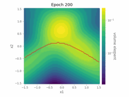
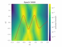
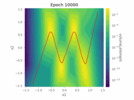
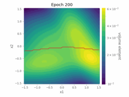
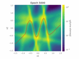
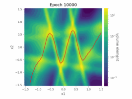
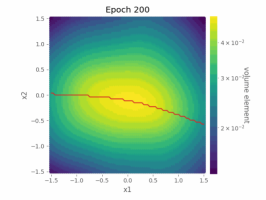
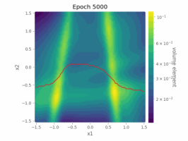
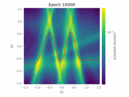
Figure 2: Evolution of the volume element over training in a network with with architecture [2, $w$, 2] for $w=5$ (first row), $w=20$ (second row), and $w=250$ (third row) hidden units across different epochs trained to classify points separated by a sinusoidal boundary $y=\frac{3}{5}\sin(7x-1)$. Red lines indicate the decision boundaries of the network. See Appendix G.1 for experimental details and additional visualizations.

6.2 Changes in geometry for shallow networks trained to classify MNIST digits

We now provide evidence that a similar phenomenon is present in networks trained to classify MNIST images. We give details of these networks in Appendix G.2; note that all reach above 95% train and test accuracy within 200 epochs. Because of the computational complexity of estimating the curvature—the Riemann tensor has $d^{2}(d^{2}-1)/12$ independent components (Misner et al., 2017; Dodson and Poston, 1991)—and its numerical sensitivity (Appendix G.1), we do not attempt to estimate it for this high-dimensional task.

In Figure 3, we plot the induced volume element at synthetic images generated by linearly interpolating between two input images (see Appendix G for details). We emphasize that linear interpolation in pixel space of course does not respect the structure of the image data, and results in unrealistic images. However, this approach has the advantage of being straightforward, and also illustrates how small Euclidean perturbations are expanded by the feature map (Novak et al., 2018). At initialization, the volume element varies without clear structure along the interpolated path. However, as training progresses, areas near the center of the path, which roughly aligns with the decision boundary, are expanded, while those near the endpoints defined by true training examples remain relatively small. This is again consistent with Hypothesis 1. We provide additional visualizations of this behavior in Appendix G.2.

To gain an understanding of the structure of the volume element beyond one-dimensional slices, in Figure 3 we also plot its value in the plane spanned by three randomly-selected example images, at points interpolated linearly within their convex hull. Here, we only show the end of training; in Appendix G.2 we show how the volume element in this plane changes over the course of training. The edges of the resulting ternary plot are one-dimensional slices like those shown in the top row of Figure 3, and we observe consistent expansion of the volume element along these paths. The volume element becomes large near the centroid of the triangle, where multiple decision boundaries intersect.

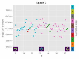
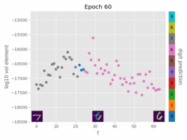
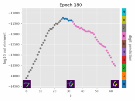
Figure 3: Top panel: $\log_{10}(\sqrt{\det g})$ induced at interpolated images between 7 and 6 by a single-hidden-layer fully-connected network trained to classify MNIST digits. Bottom panel: Digit class predictions and $\log_{10}(\sqrt{\det g})$ for the plane spanned by MNIST digits 7, 6, and 1 at the final training epoch (200) . Sample images are visualized at the endpoints and midpoint for each set. Each line is colored by its prediction at the interpolated region and end points. As training progresses, the volume elements bulge in the middle (near the decision boundary) and taper off when travelling towards endpoints. See Appendix G.2 for experimental details and Figure G.6 for images interpolated between other digits.

7 Beyond shallow learning

7.1 Deep MLPs trained on toy tasks

Thus far, we have focused on the geometry of the feature maps of single-hidden-layer neural networks. However, these analyses can also be applied to deeper networks, regarding the representation at each hidden layer as defining a feature map (Hauser and Ray, 2017; Benfenati and Marta, 2023b). As a simple version of this, in Figure 4 we consider a network with three fully-connected hidden layers trained on the sinusoid task. The metrics induced by the feature maps of all three hidden layers all show the same qualitative behavior as we observed in the shallow case in Figure 2: areas near the decision boundary are magnified. As one progresses deeper into the network, the contrast between regions of low and high magnification factor increases.

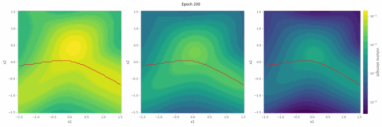
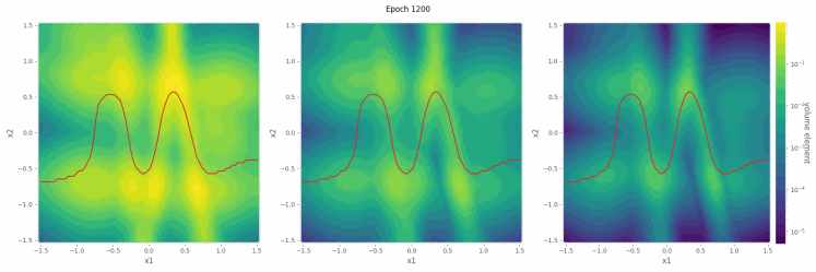
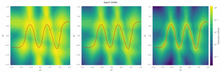
Figure 4: Evolution of the volume element over training in an architecture of [2, 8, 8, 8, 2] trained to classify points separated by a sinusoidal boundary. From left to right, each panel correspond to the feature map induced by the first, second, and third hidden layers. Red lines indicate the decision boundaries of the network. Note that the learning is performed predominantly at the first layer, and later layers offer a better demarcation by polarizing the volume elements at regions near and away from the decision boundaries. See Appendix G.1 for experimental details. More hidden units result in a better approximation to the sinusoid curve.

7.2 Deep residual networks with smooth activation functions

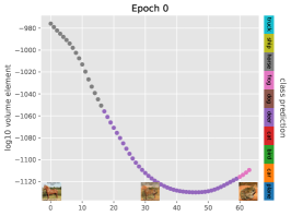
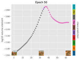
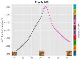
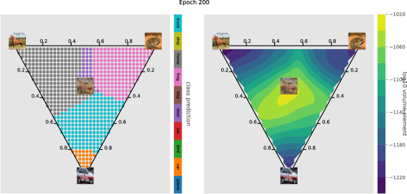
Figure 5: Top panel: $\log_{10}(\sqrt{\det g})$ induced at interpolated images between a horse and a frog by ResNet-34 with GELU activation trained to classify CIFAR-10 images. Bottom panel: Digits classification of a horse, a frog, and a car. The volume element is the largest at the intersection of several binary decision boundaries, and smallest within each of the decision region. The one-dimensional slices along the edges of each ternary plot are consistent with the top panel. See Appendix G.3 for experimental details, Figure G.14 for linear interpolation and plane spanned by other classes, and how the plane evolves during training.

As a more realistic example, we consider deep residual networks (ResNets) (He et al., 2016) trained to classify the CIFAR-10 image dataset (Krizhevsky, 2009). To make the feature map differentiable, we replace the rectified linear unit (ReLU) activation functions used in standard ResNets with Gaussian error linear units (GELUs) (Hendrycks and Gimpel, 2016). With this modification, we achieve comparable test accuracy (92%) with a ResNet-34—the largest model we can consider given computational constraints—to that obtained with ReLUs (Appendix G.3). Importantly, the feature map defined by the input-to-final-hidden-layer mapping of a ResNet-34 gives a submersion of CIFAR-10, as the input images have $32\times 32\times 3=3072$ pixels, while the final hidden layer has 512 units. Empirically, we find that the Jacobian of this mapping is full-rank (Figure G.15); we therefore consider the volume element on $(\mathcal{M}/\sim,g)$ defined by the product of the non-zero eigenvalues of the degenerate pullback metric (§2, Appendix G.3).

In Figure 5, we visualize the resulting geometry in the same way we did for networks trained on MNIST, along 1-D interpolated slices and in a 2-D interpolated plane (see Appendix G.3 for details and additional figures). In both 1-D and 2-D slices, we see a clear trend of large volume elements near decision boundaries, as we observed for shallow networks. In Figure G.20, we show that these networks also expand areas near incorrect decision boundaries, but do not expand areas along slices between three correctly-classified points of the same class. Thus, even in this more realistic setting, we observe shaping of geometry over training that appears consistent with Hypothesis 1.

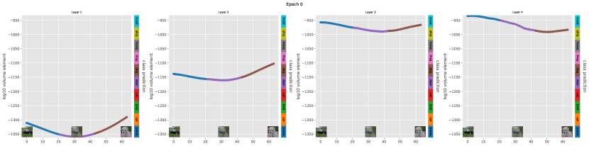
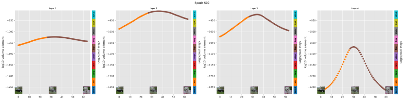
Figure 6: Visualization of volume elements across blocks of a ResNet-34 with GELU activations. Top panels: $\log_{10}(\sqrt{\det g})$ with class label predictions at interpolated samples between a car and a dog at the start of training, and from left to right lists volume elements across depth. Bottom panels: same quantities at the end of training (epoch 500). Our observation that volume elements are largest near the decision boundary is consistent across blocks, with contrast between the volume element at the test points and near the boundary increasing width depth. See Figure 7 for similar visualizations along two-dimensional slices through input space, and Appendix G.3 for experimental details.

For these deep networks, we can also study how the volume element is shaped across depth. In Figures 6 and 7, we visualize the volume element corresponding to the metric induced by pulling back the Euclidean metric on the feature space of the output of each of the four blocks of the ResNet-34. These visualizations are consistent with our general observations, with the volume element induced by each block being largest near the decision boundary. We additionally point out that the contrast between the smallest and largest volume element among the interpolated path at respective layer is least (most) pronounced at the first (last) layer, suggesting that the last layer captures the most distinguishing features across samples in different classes.

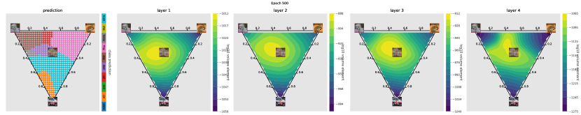
Figure 7: Visualization of volume elements across blocks of a ResNet-34 with GELU activations. Classification and volume elements of samples interpolated by a dog, a frog, and a car at the beginning of training (top panel), epoch 50 (mid panel), and epoch 500, the end of training (bottom panel). As illustrated in the one-dimensional slices in Figure 6, the volume element is consistently largest near decision boundaries, with contrast increasing with depth. See Appendix G.3 for experimental details.

7.3 Deep ReLU networks

Because of the smoothness conditions required by the definition of the pullback metric and the requirement that $(\mathcal{M},g)$ be a differentiable manifold (Hauser and Ray, 2017; Benfenati and Marta, 2023b), the approach pursued in the preceding sections does not apply directly to networks with ReLU activation functions, which are not differentiable. Deep ReLU networks are continuous piecewise-linear maps, with many distinct activation regions (Hanin and Rolnick, 2019a, b). Within each region, the corresponding linear feature map will induce a flat metric on the input space, but the magnification factor will vary from region to region. Therefore, though the overall framework of the preceding sections does not apply in the ReLU setting, we can still visualize this variation in the piecewise-constant magnification factor. In Figure 8, we replicate Figure 5 for a ResNet-34 with ReLU rather than GELU activations, and observe qualitatively similar expansion of the volume element. We provide additional visualizations of ReLU ResNets in Appendix G.3. Therefore, the qualitative picture of Hypothesis 1 can be extended beyond the globally smooth setting.

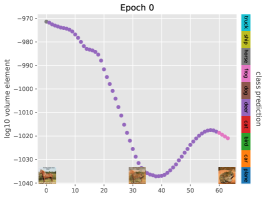
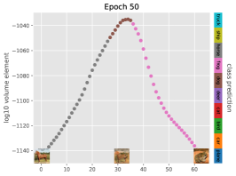
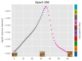
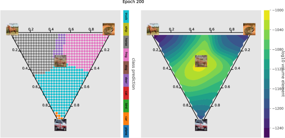
Figure 8: Top panel: $\log_{10}(\sqrt{\det g})$ induced at interpolated images between a horse and a frog by ResNet-34 with ReLU activation trained to classify CIFAR-10 images. Bottom panel: Digits classification of a horse, a frog, and a car. The volume element is the largest at the intersection of several binary decision boundaries, and smallest within each of the decision region. See Appendix G.3 for details of these experiments and additional figures.

7.4 Self-supervised learning with Barlow Twins

Though Hypothesis 1 focuses on supervised training, the same geometric analysis can be performed for any feature map, irrespective of the training procedure. To demonstrate the broader utility of visualizing the induced volume element, we consider ResNet feature maps trained with the self-supervised learning (SSL) method Barlow Twins (Zbontar et al., 2021). In Figure 9 and Appendix G.4, we show that we observe expansion of areas near the decision boundaries of a linear probe trained on top of this feature map, consistent with what we saw for supervised ResNets. In Appendix G.4, we show in contrast that a clear pattern of expansion is not visible for ResNets trained with the alternative SSL method SimCLR (Chen et al., 2020). We hypothesize that this difference results from SimCLR’s normalization of the feature map, which may make treating the embedding space as Euclidean inappropriate. These results illustrate the broader potential of our approach to give new insights into how different SSL procedures induce different geometry, suggesting avenues for future investigation.

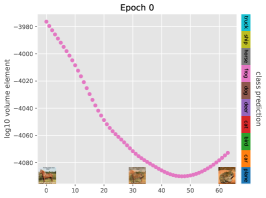
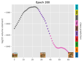
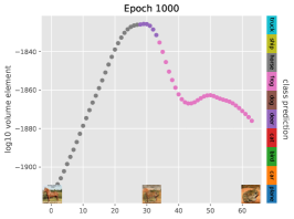
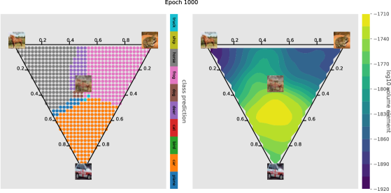
Figure 9: Top panel: $\log_{10}(\sqrt{\det g})$ induced at interpolated images between a horse and a frog by Barlow Twins with a ResNet-34 backbone with GELU activation. Bottom panel: Digits classification of a horse, a frog, and a car, prediction given by a multiclass logistic regression on the features by the ResNet backbone. The volume element is the largest at the intersection of several binary decision boundaries, and smallest within each of the decision regions. See Appendix G.4 for details of these experiments and additional figures.

8 Discussion

To conclude, we have shown that training on simple tasks shapes the Riemannian geometry induced by neural network representations by magnifying areas along decision boundaries (Amari and Wu, 1999; Wu and Amari, 2002; Williams et al., 2007). These results are relevant to the broad goal of leveraging non-Euclidean geometry in deep learning, but they differ from many past approaches in that we seek to characterize what geometric structure is learned rather than hand-engineering the optimal geometry for a given task (Bronstein et al., 2021; Weber et al., 2020).

Perhaps the most important limitation of our work is the fact that we focus either on toy tasks with two-dimensional input domains, or on low-dimensional slices through high-dimensional domains. This is a fundamental limitation of how we have attempted to visualize the geometry. As a first step towards more realistic manifolds of intermediate images, we show in Appendix G.2 that volume elements at ambiguous VAE-generated digit images from the Dirty-MNIST dataset (Mukhoti et al., 2021) are larger on average than those at clean MNIST test images. We are also restricted by computational constraints (Appendix G.3), particularly in our ability to study anisotropic measures of the geometry, such as the Ricci scalar. To characterize the geometry of state-of-the-art network architectures, more efficient and numerically stable algorithms for computing these quantities must be developed. Robustly determining the curvature of learned representations is particularly important for our overall objective of discovering useful geometric inductive biases.

An important question that we leave open for future work is whether expanding areas near decision boundaries generically improves classifier generalization, consistent with Amari and Wu (1999)’s original motivations. Indeed, it is easy to imagine a scenario in which the geometry is overfit, and the trained network becomes too sensitive to small changes in the input. This possibility is consistent with prior work on the sensitivity of deep networks (Novak et al., 2018), and with the related phenomenon of adversarial vulnerability (Szegedy et al., 2013; Goodfellow et al., 2014). Previous adversarial robustness guarantees focus on the space of network outputs (Hein and Andriushchenko, 2017; Mustafa et al., 2020; Tron et al., 2022); we believe investigating geometrically-inspired feature-space adversarial defenses is an interesting avenue for future work. In particular, we propose that this perspective could form the basis of an approach to adversarially-robust self-supervised learning, where for a given feature map one could guarantee robustness for any reasonable readout.

The question of when changes to the representational geometry are needed for good generalization can also be stated more broadly, beyond questions of local sensitivity. In a series of recent works, Radhakrishnan et al. (2022) have proposed a method for learning data-adaptive kernels, and show that for some datasets this method generalizes better than fully-trained deep networks. Concretely, their method amounts to learning a linear change of coordinates $\tilde{\mathbf{x}}=\mathbf{M}^{1/2}\mathbf{x}$ for a positive-semidefinite matrix $\mathbf{M}$, and then applying the same fixed kernel to those transformed inputs (see Appendix F for a detailed description). They focus on translation-invariant base kernels, which always induce flat, constant metrics. More generally, so long as the matrix $\mathbf{M}$ is positive-definite, this form of feature learning is simply a change of coordinates on the input space. As a form of linear masking, this method can reduce the influence of certain input channels, but it cannot affect the curvature of the embedding. In future work, it will be interesting to investigate when the flexible, nonlinear form of feature learning that reshapes the curvature of the embedding is necessary for generalization, and when it can be harmful. In this vein, it will be interesting to investigate how the notions of geometry studied here relate to measures that focus on how embeddings shape the linear separability of different classes (Chung et al., 2018; Cohen et al., 2020).

Another possible application of our ideas is to the problem of semantic data deduplication. In contemporaneous work, Abbas et al. (2023) have proposed a data pruning method that identifies related examples based on their embeddings under a pretrained feature map. Their method proceeds in two steps: first, they cluster examples using k-means based on the Euclidean distances between their embeddings, and then they eliminate examples within each cluster by identifying pairs whose embeddings have Euclidean cosine similarity above some threshold. They show that this procedure can substantially reduce the size of large image and text datasets, and that models trained on the pruned datasets display superior performance. By considering local distances between points in embedding space, their method is closely related to a finite-difference approximation of the distance as measured by the induced metric of the pretrained feature map. We therefore propose that the Riemannian viewpoint taken here could allow both for deeper understanding of existing deduplication methods and for the design of novel algorithms that are both principled and interpretable.

Finally, our results are applicable to the general problem of how to analyze and compare neural network representations (Kornblith et al., 2019; Williams et al., 2021). As illustrated by our SSL experiments, one could compute and plot the volume element induced by a feature map even when one does not have access to explicit class labels. This could allow one to study pre-trained networks for which one does not have access to the training classes, and perhaps even differentiable approximations to biological neural networks (Wang and Ponce, 2022; Acosta et al., 2022). Exploring the rich geometry induced by these networks is an exciting avenue for future investigation.

Acknowledgments and Disclosure of Funding

We thank Blake Bordelon, Matthew Farrell, Anindita Maiti, Carlos Ponce, Sabarish Sainathan, James B. Simon, and Binxu Wang for useful discussions and comments on earlier versions of our manuscript. CP and JZV were supported by NSF Award DMS-2134157 and NSF CAREER Award IIS-2239780. CP is further supported by a Sloan Research Fellowship. This work has been made possible in part by a gift from the Chan Zuckerberg Initiative Foundation to establish the Kempner Institute for the Study of Natural and Artificial Intelligence. The computations in this paper were run on the FASRC cluster supported by the FAS Division of Science Research Computing Group at Harvard University.

Appendix A Simplification of the Riemann tensor for a general shallow network

In this section, we show how the general form of the Riemann tensor can be simplified for metrics of the form considered here. As elsewhere, our conventions follow Dodson and Poston (1991). Consider a metric of the general form

$$g_{\mu\nu}=\mathbb{E}_{\mathbf{w},b}[\phi^{\prime}(\mathbf{w}\cdot\mathbf{x}+b)^{2}w_{\mu}w_{\nu}],$$ (A.1)

where we do not assume that the distribution of the weights and biases is Gaussian. For such a metric, we have

$$\partial_{\alpha}g_{\mu\nu}=2\mathbb{E}_{\mathbf{w},b}[\phi^{\prime}(\mathbf{w}\cdot\mathbf{x}+b)\phi^{\prime\prime}(\mathbf{w}\cdot\mathbf{x}+b)w_{\alpha}w_{\mu}w_{\nu}],$$ (A.2)

which is symmetric under permutation of its indices. Therefore, the Christoffel symbols of the second kind reduce to

$$\Gamma^{\alpha}_{\beta\gamma} =\frac{1}{2}g^{\alpha\mu}(\partial_{\beta}g_{\gamma\mu}-\partial_{\mu}g_{\beta\gamma}+\partial_{\gamma}g_{\mu\beta})$$ (A.3)

$$=\frac{1}{2}g^{\alpha\mu}\partial_{\beta}g_{\gamma\mu}.$$ (A.4)

The $(3,1)$ Riemann tensor is then

$$R^{\mu}_{\nu\alpha\beta} =\partial_{\alpha}\Gamma^{\mu}_{\beta\nu}-\partial_{\beta}\Gamma^{\mu}_{\alpha\nu}+\Gamma^{\rho}_{\alpha\nu}\Gamma^{\mu}_{\beta\rho}-\Gamma^{\rho}_{\beta\nu}\Gamma^{\mu}_{\alpha\rho}$$ (A.5)

$$=\frac{1}{2}\left[\partial_{\alpha}(g^{\mu\rho}\partial_{\beta}g_{\nu\rho})-\partial_{\beta}(g^{\mu\rho}\partial_{\alpha}g_{\nu\rho})\right]$$

$$\qquad+\frac{1}{4}\left[(g^{\rho\lambda}\partial_{\alpha}g_{\nu\lambda})(g^{\mu\sigma}\partial_{\beta}g_{\rho\sigma})-(g^{\rho\lambda}\partial_{\beta}g_{\nu\lambda})(g^{\mu\sigma}\partial_{\alpha}g_{\rho\sigma})\right]$$ (A.6)

$$=\frac{1}{2}\left[\partial_{\alpha}g^{\mu\rho}\partial_{\beta}g_{\nu\rho}-\partial_{\beta}g^{\mu\rho}\partial_{\alpha}g_{\nu\rho}+g^{\mu\rho}(\partial_{\alpha}\partial_{\beta}g_{\nu\rho}-\partial_{\beta}\partial_{\alpha}g_{\nu\rho})\right]$$

$$\qquad+\frac{1}{4}\left[-\partial_{\alpha}g_{\nu\lambda}\partial_{\beta}g^{\mu\lambda}+\partial_{\beta}g_{\nu\lambda}\partial_{\alpha}g^{\mu\lambda}\right]$$ (A.7)

$$=\frac{3}{4}(\partial_{\alpha}g^{\mu\rho}\partial_{\beta}g_{\nu\rho}-\partial_{\beta}g^{\mu\rho}\partial_{\alpha}g_{\nu\rho}),$$ (A.8)

where we have used the fact that partial derivatives commute and recalled the matrix calculus identity

$$\partial_{\alpha}g^{\mu\nu}=-g^{\mu\rho}g^{\nu\lambda}\partial_{\alpha}g_{\rho\lambda}.$$ (A.9)

Then, the $(4,0)$ Riemann tensor is

$$R_{\mu\nu\alpha\beta} =g_{\mu\lambda}R^{\lambda}_{\nu\alpha\beta}$$ (A.10)

$$=-\frac{3}{4}g^{\rho\lambda}(\partial_{\alpha}g_{\mu\rho}\partial_{\beta}g_{\nu\lambda}-\partial_{\beta}g_{\mu\rho}\partial_{\alpha}g_{\nu\lambda})$$ (A.11)

which, given the permutation symmetry of the derivatives of the metric, can be re-expressed as

$$R_{\mu\nu\alpha\beta} =-\frac{3}{4}g^{\rho\lambda}(\partial_{\rho}g_{\mu\alpha}\partial_{\lambda}g_{\nu\beta}-\partial_{\rho}g_{\mu\beta}\partial_{\lambda}g_{\nu\alpha}).$$ (A.12)

It is then easy to see that the simplified formula for the Riemann tensor has the expected symmetry properties under index permutation:

$$R_{\mu\nu\alpha\beta} =-R_{\mu\nu\beta\alpha}$$ (A.13)

$$R_{\mu\nu\alpha\beta} =-R_{\nu\mu\alpha\beta}$$ (A.14)

$$R_{\mu\nu\alpha\beta} =+R_{\alpha\beta\mu\nu}$$ (A.15)

and satisfies the Bianchi identity

$$R_{\mu\nu\alpha\beta}+R_{\mu\alpha\beta\nu}+R_{\mu\beta\nu\alpha}=0.$$ (A.16)

Finally, the Ricci scalar is

$$R =g^{\beta\nu}R^{\alpha}_{\nu\alpha\beta}$$ (A.17)

$$=-\frac{3}{4}g^{\mu\alpha}g^{\nu\beta}g^{\rho\lambda}(\partial_{\alpha}g_{\mu\rho}\partial_{\beta}g_{\nu\lambda}-\partial_{\beta}g_{\mu\rho}\partial_{\alpha}g_{\nu\lambda})$$ (A.18)

$$=-\frac{3}{4}g_{\rho\lambda}(\partial_{\alpha}g^{\alpha\rho}\partial_{\beta}g^{\beta\lambda}-\partial_{\beta}g^{\alpha\rho}\partial_{\alpha}g^{\beta\lambda}).$$ (A.19)

Appendix B Expansion of geometric quantities for a shallow network with fixed weights

In this appendix, we derive formulas for the geometric quantities of a finite-width shallow network with fixed weights. Our starting point is the metric (8)

$$g_{\mu\nu}=\frac{1}{n}\phi^{\prime}(z_{j})^{2}w_{j\mu}w_{j\nu},$$ (B.1)

where $z_{j}=\mathbf{w}_{j}\cdot\mathbf{x}+b_{j}$ is the preactivation of the $j$-th hidden unit.

B.1 Direct derivations for 2D inputs

As a warm-up, we first derive the geometric quantities for two-dimensional inputs ($d=2$), using simple explicit formulas for the determinant and inverse of the metric. These derivations have the same content as those in following sections for general input dimension, but are more straightforward. In this case, we will explicitly write out summations over hidden units, as we will need to exclude certain index combinations. As the metric is a $2\times 2$ symmetric matrix, we have immediately that

$$\det g =g_{11}g_{22}-g_{12}^{2}$$ (B.2)

$$=\frac{1}{n^{2}}\sum_{j,k=1}^{n}\phi^{\prime}(z_{j})^{2}\phi^{\prime}(z_{k})^{2}(w_{j1}^{2}w_{k2}^{2}-w_{j1}w_{j2}w_{k1}w_{k2})$$ (B.3)

$$=\frac{1}{n^{2}}\sum_{k\neq j}\phi^{\prime}(z_{j})^{2}\phi^{\prime}(z_{k})^{2}(w_{j1}^{2}w_{k2}^{2}-w_{j1}w_{j2}w_{k1}w_{k2})$$ (B.4)

$$=\frac{1}{n^{2}}\sum_{k<j}M_{jk}^{2}\phi^{\prime}(z_{j})^{2}\phi^{\prime}(z_{k})^{2}$$ (B.5)

$$=\frac{1}{2n^{2}}\sum_{j,k}M_{jk}^{2}\phi^{\prime}(z_{j})^{2}\phi^{\prime}(z_{k})^{2},$$ (B.6)

where we have defined

$$M_{jk}=\det\begin{pmatrix}w_{j1}&w_{j2}\\ w_{k1}&w_{k2}\end{pmatrix}=w_{j1}w_{k2}-w_{j2}w_{k1}.$$ (B.7)

This shows explicitly that the metric is invertible if and only if at least one pair of weight vectors is linearly independent, as one would intuitively expect.

Moreover, we of course have

$$g^{\mu\nu} =\frac{1}{\det g}\begin{pmatrix}g_{22}&-g_{12}\\ -g_{12}&g_{11}\end{pmatrix}.$$ (B.8)

As we are working in two dimensions, the Riemann tensor has only one independent component, and is entirely determined by the Ricci scalar (Dodson and Poston, 1991):

$$R_{\mu\nu\alpha\beta}=\frac{R}{2}(g_{\mu\alpha}g_{\nu\beta}-g_{\mu\beta}g_{\nu\alpha}).$$ (B.9)

Given the permutation symmetry of $\partial_{\alpha}g_{\mu\nu}$, we can combine the results of Appendix A with the simple formula for $g^{\mu\nu}$ to obtain

$$R =\frac{3}{2(\det g)^{2}}\bigg{[}g_{11}(\partial_{1}g_{22}\partial_{2}g_{12}-\partial_{2}g_{22}\partial_{1}g_{12})$$

$$\qquad\qquad\qquad+g_{12}(\partial_{1}g_{11}\partial_{2}g_{22}-\partial_{2}g_{11}\partial_{1}g_{22})$$

$$\qquad\qquad\qquad+g_{22}(\partial_{1}g_{12}\partial_{2}g_{11}-\partial_{2}g_{12}\partial_{1}g_{11})\bigg{]}$$ (B.10)

In general, we have

$$\partial_{\alpha}g_{\nu\rho}\partial_{\beta}g_{\lambda\gamma}-\partial_{\beta}g_{\nu\rho}\partial_{\alpha}g_{\lambda\gamma} =\frac{4}{n^{2}}\sum_{k\neq j}\phi^{\prime}(z_{j})\phi^{\prime\prime}(z_{j})\phi^{\prime}(z_{k})\phi^{\prime\prime}(z_{k})$$

$$\qquad\qquad\qquad\times(w_{j\alpha}w_{k\beta}-w_{j\beta}w_{k\alpha})w_{j\nu}w_{j\rho}w_{k\lambda}w_{k\gamma}$$ (B.11)

hence, using the fact that $M_{jj}=0$, we have

$$\frac{(\det g)^{2}}{3}R =\frac{2}{n^{3}}\sum_{i,j,k=1}^{n}M_{jk}\phi^{\prime}(z_{i})^{2}\phi^{\prime}(z_{j})\phi^{\prime}(z_{k})\phi^{\prime\prime}(z_{j})\phi^{\prime\prime}(z_{k})$$

$$\qquad\qquad\qquad\qquad\times(w_{i1}^{2}w_{j2}^{2}w_{k1}w_{k2}+w_{i1}w_{i2}w_{j1}^{2}w_{k2}^{2}+w_{i2}^{2}w_{j1}w_{j2}w_{k1}^{2})$$ (B.12)

As $M_{kj}=-M_{jk}$, we can antisymmetrize the term in the round brackets in those indices, yielding

$$\frac{(\det g)^{2}}{3}R =\frac{1}{n^{3}}\sum_{i,j,k=1}^{n}M_{jk}\phi^{\prime}(z_{i})^{2}\phi^{\prime}(z_{j})\phi^{\prime}(z_{k})\phi^{\prime\prime}(z_{j})\phi^{\prime\prime}(z_{k})$$

$$\qquad\qquad\qquad\times\bigg{[}(w_{i1}^{2}w_{j2}^{2}w_{k1}w_{k2}+w_{i1}w_{i2}w_{j1}^{2}w_{k2}^{2}+w_{i2}^{2}w_{j1}w_{j2}w_{k1}^{2})-(j\leftrightarrow k)\bigg{]}.$$ (B.13)

With a bit of algebra, we have

$$(w_{i1}^{2}w_{j2}^{2}w_{k1}w_{k2}+w_{i1}w_{i2}w_{j1}^{2}w_{k2}^{2}+w_{i2}^{2}w_{j1}w_{j2}w_{k1}^{2})-(j\leftrightarrow k) =-M_{jk}M_{ij}M_{ik}.$$ (B.14)

Therefore,

$$R =-\frac{3}{n^{3}(\det g)^{2}}\sum_{i,j,k=1}^{n}M_{jk}^{2}M_{ij}M_{ik}\phi^{\prime}(z_{i})^{2}\phi^{\prime}(z_{j})\phi^{\prime}(z_{k})\phi^{\prime\prime}(z_{j})\phi^{\prime\prime}(z_{k}).$$ (B.15)

As $M_{ii}=0$, the non-vanishing contributions to the sum are now triples of distinct indices. We remark that the index $i$ is singled out in this expression. If $n=2$, the Ricci scalar, and thus the Riemann tensor, vanishes identically. This follows from the fact that in this case the feature map is a change of coordinates on the input space (Misner et al., 2017; Dodson and Poston, 1991). If $n=3$, we have the relatively simple formula

$$R =\frac{2}{9(\det g)^{2}}M_{12}M_{23}M_{31}\phi^{\prime}(z_{1})\phi^{\prime}(z_{2})\phi^{\prime}(z_{3})$$

$$\quad\times\bigg{[}M_{23}\phi^{\prime}(z_{1})\phi^{\prime\prime}(z_{2})\phi^{\prime\prime}(z_{3})-M_{13}\phi^{\prime}(z_{2})\phi^{\prime\prime}(z_{1})\phi^{\prime\prime}(z_{3})+M_{12}\phi^{\prime}(z_{3})\phi^{\prime\prime}(z_{1})\phi^{\prime\prime}(z_{2})\bigg{]}.$$ (B.16)

B.2 The volume element

We now consider the volume element for general input dimension $d$. We use the Leibniz formula for determinants in terms of the Levi-Civita symbol $\epsilon^{\mu_{1}\cdots\mu_{d}}$ (Penrose, 2005; Misner et al., 2017):

$$\det g =\epsilon^{\mu_{1}\cdots\mu_{d}}g_{1\mu_{1}}\cdots g_{d\mu_{d}}$$ (B.17)

$$=\frac{1}{d!}\epsilon^{\mu_{1}\cdots\mu_{d}}\epsilon^{\nu_{1}\cdots\nu_{d}}g_{\mu_{1}\nu_{1}}\cdots g_{\mu_{d}\nu_{d}}.$$ (B.18)

This gives

$$\det g =\frac{1}{d!}\epsilon^{\mu_{1}\cdots\mu_{d}}\epsilon^{\nu_{1}\cdots\nu_{d}}g_{\mu_{1}\nu_{1}}\cdots g_{\mu_{d}\nu_{d}}$$ (B.19)

$$=\frac{1}{n^{d}d!}\epsilon^{\mu_{1}\cdots\mu_{d}}\epsilon^{\nu_{1}\cdots\nu_{d}}\phi^{\prime}(z_{j_{1}})^{2}\cdots\phi^{\prime}(z_{j_{d}})^{2}w_{j_{1}\mu_{1}}w_{j_{1}\nu_{1}}\cdots w_{j_{d}\mu_{d}}w_{j_{d}\nu_{d}}$$ (B.20)

$$=\frac{1}{n^{d}d!}\phi^{\prime}(z_{j_{1}})^{2}\cdots\phi^{\prime}(z_{j_{d}})^{2}(\epsilon^{\mu_{1}\cdots\mu_{d}}w_{j_{1}\mu_{1}}\cdots w_{j_{d}\mu_{d}})(\epsilon^{\nu_{1}\cdots\nu_{d}}w_{j_{1}\nu_{1}}\cdots w_{j_{d}\nu_{d}})$$ (B.21)

$$=\frac{1}{n^{d}d!}M_{j_{1}\cdots j_{d}}^{2}\phi^{\prime}(z_{j_{1}})^{2}\cdots\phi^{\prime}(z_{j_{d}})^{2},$$ (B.22)

where

$$M_{j_{1}\cdots j_{d}} =\epsilon^{\mu_{1}\cdots\mu_{d}}w_{j_{1}\mu_{1}}\cdots w_{j_{d}\mu_{d}}$$ (B.23)

$$=\det\begin{pmatrix}w_{j_{1}1}&\cdots&w_{j_{1}d}\\ \vdots&\ddots&\vdots\\ w_{j_{d}1}&\cdots&w_{j_{d}d}\end{pmatrix}$$ (B.24)

is the minor of the weight matrix obtained by selecting rows $j_{1},\ldots,j_{d}$. For $d=2$, this result agrees with that which we obtained in Appendix B.1.

B.3 The Riemann tensor and Ricci scalar

To compute the curvature for general input dimension, we need the inverse of the metric, which can be expanded using the Levi-Civita symbol as (Penrose, 2005)

$$g^{\mu\nu}=\frac{1}{(d-1)!\det g}\epsilon^{\mu\mu_{2}\cdots\mu_{d}}\epsilon^{\nu\nu_{2}\cdots\nu_{d}}g_{\mu_{2}\nu_{2}}\cdots g_{\mu_{d}\nu_{d}}.$$ (B.25)

Then, applying the results of Appendix A for

$$\partial_{\alpha}g_{\mu\nu}=\frac{2}{n}\phi^{\prime}(z_{j})\phi^{\prime\prime}(z_{j})w_{j\alpha}w_{j\mu}w_{j\nu},$$ (B.26)

the $(4,0)$ Riemann tensor is

$$R_{\mu\nu\alpha\beta} =-\frac{3}{4}g^{\rho\lambda}(\partial_{\rho}g_{\mu\alpha}\partial_{\lambda}g_{\nu\beta}-\partial_{\rho}g_{\mu\beta}\partial_{\lambda}g_{\nu\alpha})$$ (B.27)

$$=-\frac{3}{n^{d+1}(d-1)!\det g}\phi^{\prime}(z_{j_{2}})^{2}\cdots\phi^{\prime}(z_{j_{d}})^{2}\phi^{\prime}(z_{i})\phi^{\prime\prime}(z_{i})\phi^{\prime}(z_{k})\phi^{\prime\prime}(z_{k})$$

$$\quad\times\epsilon^{\rho\mu_{2}\cdots\mu_{d}}\epsilon^{\lambda\nu_{2}\cdots\nu_{d}}w_{j_{2}\mu_{2}}w_{j_{2}\nu_{2}}\cdots w_{j_{d}\mu_{d}}w_{j_{d}\nu_{d}}$$

$$\quad\times(w_{i\rho}w_{i\mu}w_{i\alpha}w_{k\lambda}w_{k\nu}w_{k\beta}-w_{i\rho}w_{i\mu}w_{i\beta}w_{k\lambda}w_{k\nu}w_{k\alpha})$$ (B.28)

$$=-\frac{3}{n^{d+1}(d-1)!\det g}\phi^{\prime}(z_{j_{2}})^{2}\cdots\phi^{\prime}(z_{j_{d}})^{2}\phi^{\prime}(z_{i})\phi^{\prime\prime}(z_{i})\phi^{\prime}(z_{k})\phi^{\prime\prime}(z_{k})$$

$$\quad\times(\epsilon^{\rho\mu_{2}\cdots\mu_{d}}w_{i\rho}w_{j_{2}\mu_{2}}\cdots w_{j_{d}\mu_{d}})(\epsilon^{\lambda\nu_{2}\cdots\nu_{d}}w_{k\lambda}w_{j_{2}\nu_{2}}\cdots w_{j_{d}\nu_{d}})$$

$$\quad\times(w_{i\mu}w_{i\alpha}w_{k\nu}w_{k\beta}-w_{i\mu}w_{i\beta}w_{k\nu}w_{k\alpha})$$ (B.29)

$$=-\frac{3}{n^{d+1}(d-1)!\det g}\phi^{\prime}(z_{j_{2}})^{2}\cdots\phi^{\prime}(z_{j_{d}})^{2}\phi^{\prime}(z_{i})\phi^{\prime\prime}(z_{i})\phi^{\prime}(z_{k})\phi^{\prime\prime}(z_{k})$$

$$\quad\times M_{ij_{2}\cdots j_{d}}M_{kj_{2}\cdots j_{d}}w_{i\mu}w_{k\nu}(w_{i\alpha}w_{k\beta}-w_{i\beta}w_{k\alpha}).$$ (B.30)

Raising one index, the $(3,1)$ Riemann tensor is

$$R^{\lambda}_{\nu\alpha\beta} =g^{\lambda\mu}R_{\mu\nu\alpha\beta}$$ (B.31)

$$=-\frac{3}{n^{2}[n^{d-1}(d-1)!\det g]^{2}}$$

$$\quad\times\phi^{\prime}(z_{l_{2}})^{2}\cdots\phi^{\prime}(z_{l_{d}})^{2}\phi^{\prime}(z_{j_{2}})^{2}\cdots\phi^{\prime}(z_{j_{d}})^{2}\phi^{\prime}(z_{i})\phi^{\prime\prime}(z_{i})\phi^{\prime}(z_{k})\phi^{\prime\prime}(z_{k})$$

$$\quad\times M_{ij_{2}\cdots j_{d}}M_{kj_{2}\cdots j_{d}}M_{il_{2}\cdots l_{d}}\epsilon^{\lambda\nu_{2}\cdots\nu_{d}}w_{l_{2}\nu_{2}}\cdots w_{l_{d}\nu_{d}}w_{k\nu}(w_{i\alpha}w_{k\beta}-w_{i\beta}w_{k\alpha})$$ (B.32)

hence the Ricci tensor is

$$R_{\nu\beta} =R^{\lambda}_{\nu\lambda\beta}$$ (B.33)

$$=-\frac{3}{n^{2}[n^{d-1}(d-1)!\det g]^{2}}\phi^{\prime}(z_{j_{2}})^{2}\cdots\phi^{\prime}(z_{j_{d}})^{2}\phi^{\prime}(z_{l_{2}})^{2}\cdots\phi^{\prime}(z_{l_{d}})^{2}$$

$$\quad\times\phi^{\prime}(z_{i})\phi^{\prime\prime}(z_{i})\phi^{\prime}(z_{k})\phi^{\prime\prime}(z_{k})$$

$$\quad\times M_{ij_{2}\cdots j_{d}}M_{kj_{2}\cdots j_{d}}M_{il_{2}\cdots l_{d}}w_{k\nu}(M_{il_{2}\cdots l_{d}}w_{k\beta}-w_{i\beta}M_{kl_{2}\cdots l_{d}}).$$ (B.34)

Finally, the Ricci scalar is

$$R =g^{\nu\beta}R_{\nu\beta}$$ (B.35)

$$=-\frac{3}{n^{2}[n^{d-1}(d-1)!\det g]^{3}}$$

$$\quad\times\phi^{\prime}(z_{i})\phi^{\prime\prime}(z_{i})\phi^{\prime}(z_{j})\phi^{\prime\prime}(z_{j})\phi^{\prime}(z_{k_{2}})^{2}\cdots\phi^{\prime}(z_{k_{d}})^{2}\phi^{\prime}(z_{l_{2}})^{2}\cdots\phi^{\prime}(z_{l_{d}})^{2}\phi^{\prime}(z_{m_{2}})^{2}\cdots\phi^{\prime}(z_{m_{d}})^{2}$$

$$\quad\times M_{ik_{2}\cdots k_{d}}M_{jk_{2}\cdots k_{d}}(M_{il_{2}\cdots l_{d}}^{2}M_{jm_{2}\cdots m_{d}}^{2}-M_{il_{2}\cdots l_{d}}M_{jl_{2}\cdots l_{d}}M_{im_{2}\cdots m_{d}}M_{jm_{2}\cdots m_{d}}).$$ (B.36)

We now observe that the quantity outside the round brackets is symmetric under interchanging $l_{\mu}\leftrightarrow m_{\mu}$, hence we may symmetrize the quantity in the round brackets, which, as

$$(M_{il_{2}\cdots l_{d}}^{2}M_{jm_{2}\cdots m_{d}}^{2}-M_{il_{2}\cdots l_{d}}M_{jl_{2}\cdots l_{d}}M_{im_{2}\cdots m_{d}}M_{jm_{2}\cdots m_{d}})+(l_{\mu}\leftrightarrow m_{\mu})$$ (B.37)

$$=M_{il_{2}\cdots l_{d}}^{2}M_{jm_{2}\cdots m_{d}}^{2}+M_{im_{1}\cdots m_{d}}^{2}M_{jl_{2}\cdots l_{d}}^{2}-2M_{il_{2}\cdots l_{d}}M_{jl_{2}\cdots l_{d}}M_{im_{2}\cdots m_{d}}M_{jm_{2}\cdots m_{d}}$$ (B.38)

$$=(M_{il_{2}\cdots l_{d}}M_{jm_{2}\cdots m_{d}}-M_{im_{2}\cdots m_{d}}M_{jl_{2}\cdots l_{d}})^{2},$$ (B.39)

yields

$$R =-\frac{3}{2n^{2}[n^{d-1}(d-1)!\det g]^{3}}\phi^{\prime}(z_{i})\phi^{\prime\prime}(z_{i})\phi^{\prime}(z_{j})\phi^{\prime\prime}(z_{j})\phi^{\prime}(z_{k_{2}})^{2}\cdots\phi^{\prime}(z_{k_{d}})^{2}M_{ik_{2}\cdots k_{d}}M_{jk_{2}\cdots k_{d}}$$

$$\quad\times\phi^{\prime}(z_{l_{2}})^{2}\cdots\phi^{\prime}(z_{l_{d}})^{2}\phi^{\prime}(z_{m_{2}})^{2}\cdots\phi^{\prime}(z_{m_{d}})^{2}(M_{il_{2}\cdots l_{d}}M_{jm_{2}\cdots m_{d}}-M_{im_{2}\cdots m_{d}}M_{jl_{2}\cdots l_{d}})^{2}.$$ (B.40)

If $d=2$, we can show by direct computation that

$$M_{il}M_{jm}-M_{im}M_{jl}=M_{ij}M_{lm},$$ (B.41)

hence this result simplifies to

$$R =-\frac{3}{2n^{5}[\det g]^{3}}\phi^{\prime}(z_{i})\phi^{\prime\prime}(z_{i})\phi^{\prime}(z_{j})\phi^{\prime\prime}(z_{j})\phi^{\prime}(z_{k})^{2}M_{ik}M_{jk}M_{ij}^{2}$$

$$\quad\times\phi^{\prime}(z_{l})^{2}\phi^{\prime}(z_{m})^{2}M_{lm}^{2}$$ (B.42)

$$=-\frac{3}{n^{3}(\det g)^{2}}\phi^{\prime}(z_{i})\phi^{\prime\prime}(z_{i})\phi^{\prime}(z_{j})\phi^{\prime\prime}(z_{j})\phi^{\prime}(z_{k})^{2}M_{ik}M_{jk}M_{ij}^{2},$$ (B.43)

which recovers the formula (B.15) we obtained in Appendix B.1.

B.4 Example: error function activations

In this section, we perform explicit computations for error function activations $\phi(x)=\operatorname{erf}(x/\sqrt{2})$. In this case, $\phi^{\prime}(x)=\sqrt{2/\pi}\exp(-x^{2}/2)$, so

$$\det g =\frac{1}{n^{d}d!}M_{j_{1}\cdots j_{d}}^{2}\phi^{\prime}(z_{j_{1}})^{2}\cdots\phi^{\prime}(z_{j_{d}})^{2}$$ (B.44)

$$=\frac{1}{d!}\left(\frac{2}{\pi n}\right)^{d}M_{j_{1}\cdots j_{d}}^{2}\exp[-(z_{j_{1}}^{2}+\cdots+z_{j_{d}}^{2})].$$ (B.45)

Each contribution to this sum is a Gaussian bump, which we write as

$$\exp[-(z_{j_{1}}^{2}+\cdots+z_{j_{d}}^{2})]=\exp\left[-(Q_{j_{1}\cdots j_{d}})_{\mu\nu}[x_{\mu}-(c_{j_{1}\cdots j_{d}})_{\mu}][x_{\nu}-(c_{j_{1}\cdots j_{d}})_{\nu}]\right]$$ (B.46)

for a $d\times d$ precision matrix $\mathbf{Q}_{j_{1}\cdots j_{d}}$ and a center point $\mathbf{c}_{j_{1}\cdots j_{d}}$. Expanding out the sum of squares in the exponential, we have

$$z_{j_{1}}^{2}+\cdots+z_{j_{d}}^{2} =(w_{j_{1}\mu}x_{\mu}+b_{j_{1}})^{2}+\cdots+(w_{j_{d}\mu}x_{\mu}+b_{j_{d}})^{2}$$ (B.47)

$$=(w_{j_{1}\mu}w_{j_{1}\nu}+\cdots+w_{j_{d}\mu}w_{j_{d}\nu})x_{\mu}x_{\nu}$$

$$\quad+2(b_{j_{1}}w_{j_{1}\mu}+\cdots+b_{j_{d}}w_{j_{d}\mu})x_{\mu}$$

$$\quad+(b_{j_{1}}^{2}+\cdots+b_{j_{d}}^{2}),$$ (B.48)

from which we can see that the precision matrix is

$$(Q_{j_{1}\cdots j_{d}})_{\mu\nu}=w_{j_{1}\mu}w_{j_{1}\nu}+\cdots+w_{j_{d}\mu}w_{j_{d}\nu},$$ (B.49)

while the center point is given by $(c_{j_{1}\cdots j_{d}})_{\mu}=-(Q_{j_{1}\cdots j_{d}}^{-1})_{\mu\nu}(b_{j_{1}}w_{j_{1}\nu}+\cdots+b_{j_{d}}w_{j_{d}\nu})$. Using the Leibniz formula for determinants (B.17), we have

$$\det Q_{j_{1}\cdots j_{d}} =\frac{1}{d!}\epsilon^{\mu_{1}\cdots\mu_{d}}\epsilon^{\nu_{1}\cdots\nu_{d}}(Q_{j_{1}\cdots j_{d}})_{\mu_{1}\nu_{1}}\cdots(Q_{j_{1}\cdots j_{d}})_{\mu_{d}\nu_{d}}$$ (B.50)

$$=\frac{1}{d!}\sum_{i_{1},\cdots,i_{d}=1}^{d}\epsilon^{\mu_{1}\cdots\mu_{d}}\epsilon^{\nu_{1}\cdots\nu_{d}}w_{j_{i_{1}}\mu_{1}}w_{j_{i_{1}}\nu_{1}}\cdots w_{j_{i_{d}}\mu_{d}}w_{j_{i_{d}}\nu_{d}}$$ (B.51)

$$=\frac{1}{d!}\sum_{i_{1},\cdots,i_{d}=1}^{d}(\epsilon^{\mu_{1}\cdots\mu_{d}}w_{j_{i_{1}}\mu_{1}}\cdots w_{j_{i_{d}}\mu_{d}})(\epsilon^{\nu_{1}\cdots\nu_{d}}w_{j_{i_{1}}\nu_{1}}\cdots w_{j_{i_{d}}\nu_{d}})$$ (B.52)

$$=\frac{1}{d!}\sum_{i_{1},\cdots,i_{d}=1}^{d}(\epsilon^{j_{i_{1}}\cdots j_{i_{d}}})^{2}M_{j_{1}\cdots j_{d}}^{2}$$ (B.53)

$$=M_{j_{1}\cdots j_{d}}^{2},$$ (B.54)

hence we may write

$$\det g =\frac{1}{d!}\left(\frac{2}{\pi n}\right)^{d}\det(Q_{j_{1}\cdots j_{d}})\exp\bigg{(}-(Q_{j_{1}\cdots j_{d}})_{\mu\nu}[x_{\mu}-(c_{j_{1}\cdots j_{d}})_{\mu}][x_{\nu}-(c_{j_{1}\cdots j_{d}})_{\nu}]\bigg{)}.$$ (B.55)

If all the bias terms are zero, then the bump must be centered at the origin.

If the bias terms do not vanish, then the center point is

$$(c_{j_{1}\cdots j_{d}})_{\mu}$$

$$=-(Q_{j_{1}\cdots j_{d}}^{-1})_{\mu\nu}(b_{j_{1}}w_{j_{1}\nu}+\cdots+b_{j_{d}}w_{j_{d}\nu})$$ (B.56)

$$=-\frac{1}{(d-1)!\det Q_{j_{1}\cdots j_{d}}}\sum_{i_{1},\cdots,i_{d}=1}^{d}\epsilon^{\mu\mu_{2}\cdots\mu_{d}}\epsilon^{\nu\nu_{2}\cdots\nu_{d}}w_{j_{i_{2}}\mu_{2}}w_{j_{i_{2}}\nu_{2}}\cdots w_{j_{i_{d}}\mu_{d}}w_{j_{i_{d}}\nu_{d}}b_{j_{i_{1}}}w_{j_{i_{1}}\mu}$$ (B.57)

$$=-\frac{1}{(d-1)!\det Q_{j_{1}\cdots j_{d}}}M_{j_{1}\cdots j_{d}}\sum_{i_{1},\cdots,i_{d}=1}^{d}\epsilon^{\nu\nu_{2}\cdots\nu_{d}}w_{j_{i_{2}}\nu_{2}}\cdots w_{j_{i_{d}}\nu_{d}}b_{j_{i_{1}}}\epsilon^{j_{i_{1}}\cdots j_{i_{d}}}$$ (B.58)

$$=-\frac{1}{(d-1)!M_{j_{1}\cdots j_{d}}}\sum_{i_{1},\cdots,i_{d}=1}^{d}\epsilon^{\nu\nu_{2}\cdots\nu_{d}}\epsilon^{j_{i_{1}}\cdots j_{i_{d}}}b_{j_{i_{1}}}w_{j_{i_{2}}\nu_{2}}\cdots w_{j_{i_{d}}\nu_{d}}$$ (B.59)

$$=-\frac{1}{(d-1)!M_{j_{1}\cdots j_{d}}}\epsilon^{\nu\nu_{2}\cdots\nu_{d}}B_{j_{1}\cdots j_{d},\nu_{2}\cdots\nu_{d}}$$ (B.60)

where we let

$$B_{j_{1}\cdots j_{d},\nu_{2}\cdots\nu_{d}}=\det\begin{pmatrix}b_{j_{1}}&w_{j_{1}\nu_{2}}&\cdots&w_{j_{1}\nu_{d}}\\ b_{j_{2}}&w_{j_{2}\nu_{2}}&\cdots&w_{j_{2}\nu_{d}}\\ \vdots&\vdots&\ddots&\vdots\\ b_{j_{d}}&w_{j_{d}\nu_{2}}&\cdots&w_{j_{d}\nu_{d}}\end{pmatrix}.$$ (B.61)

In general, this is not particularly useful.

In the special case of two-dimensional inputs, we have

$$\det g =\left(\frac{2}{\pi n}\right)^{2}\sum_{j<k}\det(Q_{jk})\exp\bigg{(}-(Q_{jk})_{\mu\nu}[x_{\mu}-(c_{jk})_{\mu}][x_{\nu}-(c_{jk})_{\nu}]\bigg{)}.$$ (B.62)

for center

$$\mathbf{c}_{jk}=\frac{1}{M_{jk}}\begin{pmatrix}-(b_{j}w_{k2}-b_{k}w_{j2})\\ b_{j}w_{k1}-b_{k}w_{j1}\end{pmatrix}$$ (B.63)

and precision matrix

$$\mathbf{Q}_{jk}=\begin{pmatrix}w_{j1}^{2}+w_{k1}^{2}&w_{j1}w_{j2}+w_{k1}w_{k2}\\ w_{j1}w_{j2}+w_{k1}w_{k2}&w_{i2}^{2}+w_{j2}^{2}\end{pmatrix}.$$ (B.64)

As $\phi^{\prime\prime}(x)=-\sqrt{2/\pi}x\exp(-x^{2}/2)$, the Ricci curvature has a similar expansion in terms of Gaussian bumps, but the bumps are now modulated by products of preactivations.

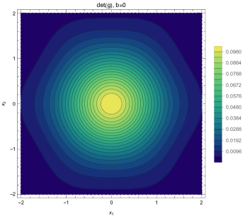
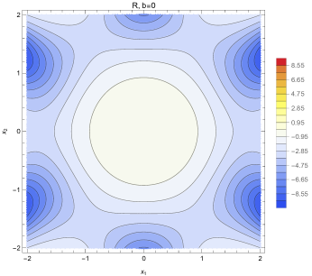
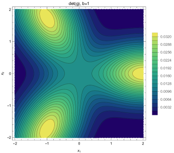
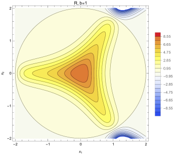
Figure B.1: Volume element (left) and Ricci scalar $R$ (right) for erf networks with three hidden units on the unit circle and bias zero (top) or one (bottom). See text for full description of the setup.

As an illustrative example, consider an erf network with three hidden units, with biases uniformly equal to $b$ and weight matrix

$$\mathbf{W}=\begin{pmatrix}1&0\\ -1/2&\sqrt{3}/2\\ -1/2&-\sqrt{3}/2\end{pmatrix}.$$ (B.65)

In this case, there are three unique pairs of weights that contribute to the volume element: $12$, $23$, and $13$. We can easily see that $M_{12}=M_{23}=-M_{13}=+\sqrt{3}/2$, and then that the bump centers are at

$$\mathbf{c}_{12}=b\begin{pmatrix}-1\\ -\sqrt{3}\end{pmatrix},\quad\mathbf{c}_{23}=b\begin{pmatrix}+2\\ 0\end{pmatrix},\quad\textrm{and}\quad\mathbf{c}_{13}=b\begin{pmatrix}-1\\ +\sqrt{3}\end{pmatrix}.$$ (B.66)

with precision matrices

$$\mathbf{Q}_{12}=\begin{pmatrix}5/4&-\sqrt{3}/4\\ -\sqrt{3}/4&5/4\end{pmatrix},\quad\mathbf{Q}_{12}=\begin{pmatrix}1/2&0\\ 0&3/2\end{pmatrix},\quad\textrm{and}\quad\mathbf{Q}_{12}=\begin{pmatrix}5/4&\sqrt{3}/4\\ \sqrt{3}/4&5/4\end{pmatrix}.$$ (B.67)

We can also explicitly write out

$$\det g=\frac{1}{3\pi^{2}}e^{-\frac{3}{2}(\|\mathbf{x}\|^{2}+2b^{2})}\left[e^{(x_{1}+b)^{2}}+e^{\frac{1}{4}(x_{1}+\sqrt{3}x_{2}-2b)^{2}}+e^{\frac{1}{4}(x_{1}-\sqrt{3}x_{2}-2b)^{2}}\right].$$ (B.68)

Therefore, the volume element has a three-fold rotational symmetry for $b>0$, and six-fold symmetry for $b=0$. Considering the Ricci scalar, we can use the explicit formula obtained for three hidden units in Appendix B.1 to work out that

$$R =-\frac{1}{\pi^{3}(\det g)^{2}}(\|\mathbf{x}\|^{2}-4b^{2})e^{-\frac{3}{2}(\|\mathbf{x}\|^{2}+2b^{2})}$$ (B.69)

$$=-\frac{9\pi}{4}\frac{(\|\mathbf{x}\|^{2}-4b^{2})e^{\frac{3}{2}(\|\mathbf{x}\|^{2}+2b^{2})}}{\left[e^{(x_{1}+b)^{2}}+e^{\frac{1}{4}(x_{1}+\sqrt{3}x_{2}-2b)^{2}}+e^{\frac{1}{4}(x_{1}-\sqrt{3}x_{2}-2b)^{2}}\right]^{2}}.$$ (B.70)

Again, the Ricci scalar has six-fold symmetry if $b=0$, and three-fold symmetry if $b>0$. We visualize this behavior in Figure B.1.

Appendix C Derivation of geometric quantities at infinite width

In this section, we derive the geometric quantities for the infinite-width metric (or, equivalently, the average finite-width metric) at initialization:

$$g_{\mu\nu}=\mathbb{E}_{\mathbf{w}\sim\mathcal{N}(\mathbf{0},\sigma^{2}\mathbf{I}_{d}),b\sim\mathcal{N}(0,\zeta^{2})}[\phi^{\prime}(\mathbf{w}\cdot\mathbf{x}+b)^{2}w_{\mu}w_{\nu}].$$ (C.1)

For the remainder of this section, we will simply write the expectation over $\mathbf{w}\sim\mathcal{N}(\mathbf{0},\sigma^{2}\mathbf{I}_{d})$ and $b\sim\mathcal{N}(0,\zeta^{2})$ as $\mathbb{E}[\cdot]$. We let

$$z\equiv\mathbf{w}\cdot\mathbf{x}+b,$$ (C.2)

which has an induced $\mathcal{N}(0,\sigma^{2}\|\mathbf{x}\|^{2}+\zeta^{2})$ distribution. We remark that it is easy to show that (C.1) is the metric induced by the NNGP kernel

$$k(\mathbf{x},\mathbf{y})=\mathbb{E}[\phi(\mathbf{w}\cdot\mathbf{x}+b)\phi(\mathbf{w}\cdot\mathbf{y}+b)]$$ (C.3)

using the formula (Burges, 1999)

$$g_{\mu\nu}=\frac{1}{2}\frac{\partial^{2}}{\partial x_{\mu}\partial x_{\nu}}k(\mathbf{x},\mathbf{x})-\left[\frac{\partial^{2}}{\partial y_{\mu}\partial y_{\nu}}k(\mathbf{x},\mathbf{y})\right]_{\mathbf{y}=\mathbf{x}}$$ (C.4)

for a sufficiently smooth activation function. We note also that here the differentiability conditions may be relaxed to weak differentiability conditions (Daniely et al., 2016; Zavatone-Veth et al., 2021).

Applying Stein’s lemma twice, we have

$$g_{\mu\nu} =\mathbb{E}[\phi^{\prime}(z)^{2}w_{\mu}w_{\nu}]$$ (C.5)

$$=\sigma^{2}\mathbb{E}[\phi^{\prime}(z)^{2}]\delta_{\mu\nu}+2\sigma^{2}\mathbb{E}[\phi^{\prime}(z)\phi^{\prime\prime}(z)w_{\nu}]x_{\mu}$$ (C.6)

$$=\sigma^{2}\mathbb{E}[\phi^{\prime}(z)^{2}]\delta_{\mu\nu}+2\sigma^{4}\mathbb{E}[\phi^{\prime\prime}(z)^{2}+\phi^{\prime}(z)\phi^{\prime\prime\prime}(z)]x_{\mu}x_{\nu}.$$ (C.7)

Then, we can see that the metric is of a special form. Noting that $\mathbb{E}[\phi^{\prime}(z)^{2}]\geq 0$ and that

$$\sigma^{2}\mathbb{E}[\phi^{\prime\prime}(z)^{2}+\phi^{\prime}(z)\phi^{\prime\prime\prime}(z)] =\sigma^{2}\frac{d}{d(\sigma^{2}\|\mathbf{x}\|^{2}+\zeta^{2})}\mathbb{E}[\phi^{\prime}(z)^{2}]$$ (C.8)

$$=\frac{d}{d\|\mathbf{x}\|^{2}}\mathbb{E}[\phi^{\prime}(z)^{2}]$$ (C.9)

by Price’s theorem (Price, 1958) and the chain rule, we may write

$$g_{\mu\nu} =e^{\Omega(\|\mathbf{x}\|^{2})}[\delta_{\mu\nu}+2\Omega^{\prime}(\|\mathbf{x}\|^{2})x_{\mu}x_{\nu}],$$ (C.10)

where we have defined the function $\Omega(\|\mathbf{x}\|^{2})$ by

$$\exp\Omega(\|\mathbf{x}\|^{2})\equiv\sigma^{2}\mathbb{E}[\phi^{\prime}(z)^{2}].$$ (C.11)

C.1 Geometric quantities for metrics of the form induced by the shallow NNGP kernel

Motivated by the metric induced by the shallow NNGP kernel, we consider metrics of the general form

$$g_{\mu\nu}=e^{\Omega(\|\mathbf{x}\|^{2})}[\delta_{\mu\nu}+2\Omega^{\prime}(\|\mathbf{x}\|^{2})x_{\mu}x_{\nu}],$$ (C.12)

where $\Omega$ is a smooth function with derivative $\Omega^{\prime}$. For brevity, we will henceforth suppress the argument of $\Omega$.

Such metrics have determinant

$$\det g=e^{d\Omega}(1+2\|\mathbf{x}\|^{2}\Omega^{\prime})$$ (C.13)

by the matrix determinant lemma, and inverse

$$g^{\mu\nu}=e^{-\Omega}\left[\delta_{\mu\nu}-\frac{2\Omega^{\prime}}{1+2\|\mathbf{x}\|^{2}\Omega^{\prime}}x_{\mu}x_{\nu}\right]$$ (C.14)

by the Sherman-Morrison formula. It is also easy to see that the eigenvalues of the metric at any given point $\mathbf{x}$ are $e^{\Omega}(1+2\|\mathbf{x}\|^{2}\Omega^{\prime})$ with corresponding eigenvector $\mathbf{x}/\|\mathbf{x}\|$, and $e^{\Omega}$ with multiplicity $d-1$, with eigenvectors lying in the null space of $\mathbf{x}$.

We now consider the Riemann tensor. For such metrics, we have

$$\partial_{\alpha}g_{\mu\nu}=2e^{\Omega}\Omega^{\prime}(x_{\alpha}\delta_{\mu\nu}+x_{\mu}\delta_{\alpha\nu}+x_{\nu}\delta_{\alpha\mu})+4e^{\Omega}[\Omega^{\prime\prime}+(\Omega^{\prime})^{2}]x_{\alpha}x_{\mu}x_{\nu},$$ (C.15)

which is symmetric under permutation of its indices. Then, we may use the simplified formula for the $(4,0)$ Riemann tensor obtained in Appendix A, which yields

$$R_{\mu\nu\alpha\beta} =-\frac{3e^{\Omega}(\Omega^{\prime})^{2}}{1+2\|\mathbf{x}\|^{2}\Omega^{\prime}}\left[\|\mathbf{x}\|^{2}\delta_{\mu\alpha}\delta_{\nu\beta}+\left(1+2\|\mathbf{x}\|^{2}\frac{\Omega^{\prime\prime}}{\Omega^{\prime}}\right)(x_{\nu}x_{\beta}\delta_{\mu\alpha}+x_{\mu}x_{\alpha}\delta_{\nu\beta})-(\alpha\leftrightarrow\beta)\right]$$ (C.16)

after a straightforward computation, where we have noted that

$$g^{\rho\lambda}x_{\rho}=e^{-\Omega}\frac{1}{1+2\|\mathbf{x}\|^{2}\Omega^{\prime}}x_{\lambda}$$ (C.17)

and

$$g^{\rho\lambda}x_{\rho}x_{\lambda}=e^{-\Omega}\frac{\|\mathbf{x}\|^{2}}{1+2\|\mathbf{x}\|^{2}\Omega^{\prime}}$$ (C.18)

We can then compute the Ricci scalar

$$R =g^{\mu\alpha}g^{\nu\beta}R_{\mu\nu\alpha\beta}$$ (C.19)

$$=-\frac{3e^{\Omega}(\Omega^{\prime})^{2}}{1+2\|\mathbf{x}\|^{2}\Omega^{\prime}}\bigg{[}\|\mathbf{x}\|^{2}(g^{\alpha\alpha}g^{\beta\beta}-g^{\alpha\beta}g^{\beta\alpha})$$

$$\qquad\qquad\qquad\qquad+2\left(1+2\|\mathbf{x}\|^{2}\frac{\Omega^{\prime\prime}}{\Omega^{\prime}}\right)(g^{\alpha\alpha}g^{\nu\beta}x_{\nu}x_{\beta}-g^{\mu\alpha}g^{\mu\beta}x_{\alpha}x_{\beta})\bigg{]}$$ (C.20)

which, as

$$g^{\alpha\alpha}g^{\beta\beta}-g^{\alpha\beta}g^{\beta\alpha} =e^{-2\Omega}\left(d-2\frac{2\|\mathbf{x}\|^{2}\Omega^{\prime}}{1+2\|\mathbf{x}\|^{2}\Omega^{\prime}}\right)(d-1)$$ (C.21)

and

$$g^{\alpha\alpha}g^{\nu\beta}x_{\nu}x_{\beta}-g^{\mu\alpha}g^{\mu\beta}x_{\alpha}x_{\beta} =e^{-2\Omega}\frac{\|\mathbf{x}\|^{2}}{1+2\|\mathbf{x}\|^{2}\Omega^{\prime}}(d-1)$$ (C.22)

yields

$$R=-\frac{3(d-1)e^{-\Omega}(\Omega^{\prime})^{2}\|\mathbf{x}\|^{2}}{(1+2\|\mathbf{x}\|^{2}\Omega^{\prime})^{2}}\left[d+2+2\|\mathbf{x}\|^{2}\left((d-2)\Omega^{\prime}+2\frac{\Omega^{\prime\prime}}{\Omega^{\prime}}\right)\right].$$ (C.23)

C.2 Examples

As an analytically-tractable example, we consider the error function $\phi(x)=\operatorname{erf}(x/\sqrt{2})$. For such networks, the NNGP kernel is

$$k(\mathbf{x},\mathbf{y})=\frac{2}{\pi}\arcsin\frac{\sigma^{2}\mathbf{x}\cdot\mathbf{y}+\zeta^{2}}{\sqrt{(1+\sigma^{2}\|\mathbf{x}\|^{2}+\zeta^{2})(1+\sigma^{2}\|\mathbf{y}\|^{2}+\zeta^{2})}},$$ (C.24)

which is easy to prove using the integral representation of the error function (Saad and Solla, 1995). In this case, we have the simple result $\phi^{\prime}(x)=\sqrt{2/\pi}\exp(-x^{2}/2)$, hence we can easily compute

$$\mathbb{E}[\phi^{\prime}(z)^{2}] =\frac{2}{\pi\sqrt{1+2(\sigma^{2}\|\mathbf{x}\|^{2}+\zeta^{2})}}.$$ (C.25)

This yields

$$\Omega(\|\mathbf{x}\|^{2})=-\frac{1}{2}\log[1+2(\sigma^{2}\|\mathbf{x}\|^{2}+\zeta^{2})]+\log\frac{2\sigma^{2}}{\pi}$$ (C.26)

hence we easily obtain the volume element

$$\sqrt{\det g}=\left(\frac{2\sigma^{2}}{\pi}\right)^{d/2}\frac{\sqrt{2\zeta^{2}+1}}{[1+2(\sigma^{2}\|\mathbf{x}\|^{2}+\zeta^{2})]^{(d+2)/4}}$$ (C.27)

and the Ricci scalar

$$R=-\frac{3\pi(d-1)(d+2)\sigma^{2}\|\mathbf{x}\|^{2}}{2(2\zeta^{2}+1)\sqrt{1+2(\sigma^{2}\|\mathbf{x}\|^{2}+\zeta^{2})}}.$$ (C.28)

In this case, it is easy to see that $R$ is negative for all $d>1$ and that it is a monotonically decreasing function of $\|\mathbf{x}\|$, hence curvature becomes increasingly negative with increasing radius.

Another illustrative example is the monomial $\phi(x)=x^{q}/\sqrt{(2q-1)!!}$ for integer $q\geq 1$, normalized such that

$$k(\mathbf{x},\mathbf{x})=\frac{1}{(2q-1)!!}\mathbb{E}[z^{2q}]=(\sigma^{2}\|\mathbf{x}\|^{2}+\zeta^{2})^{q}.$$ (C.29)

Though this is not required to obtain the metric, an explicit formula for the NNGP kernel for two distinct inputs can be obtained using the Mehler expansion of the bivariate Gaussian density (Daniely et al., 2016; Zavatone-Veth and Pehlevan, 2021), or by direct computation using Isserlis’ theorem (Zavatone-Veth et al., 2021). Following the first approach, we expand the kernel as

$$k(\mathbf{x},\mathbf{y}) =\frac{1}{(2q-1)!!}\mathbb{E}_{\mathbf{w},b}[(\mathbf{w}\cdot\mathbf{x}+b)^{q}(\mathbf{w}\cdot\mathbf{y}+b)^{q}]$$ (C.30)

$$=[(\sigma^{2}\|\mathbf{x}\|^{2}+\zeta^{2})(\sigma^{2}\|\mathbf{y}\|^{2}+\zeta^{2})]^{q/2}\frac{1}{(2q-1)!!}\mathbb{E}[u^{q}v^{q}],$$ (C.31)

where we have

$$\begin{pmatrix}u\\ v\end{pmatrix}\sim\mathcal{N}\left(\begin{pmatrix}0\\ 0\end{pmatrix},\begin{pmatrix}1&\rho\\ \rho&1\end{pmatrix}\right)$$ (C.32)

for

$$\rho=\frac{\sigma^{2}\mathbf{x}\cdot\mathbf{y}+\zeta^{2}}{\sqrt{(\sigma^{2}\|\mathbf{x}\|^{2}+\zeta^{2})(\sigma^{2}\|\mathbf{y}\|^{2}+\zeta^{2})}}.$$ (C.33)

Then, using the Mehler expansion, we have

$$\mathbb{E}[u^{q}v^{q}] =\sum_{k=0}^{\infty}\frac{\rho^{k}}{k!}\mathbb{E}_{t\sim\mathcal{N}(0,1)}[He_{k}(t)t^{q}]^{2}$$ (C.34)

where $He_{k}(t)$ is the $k$-th probabilist’s Hermite polynomial. Using the inversion formula

$$t^{q}=q!\sum_{m=0}^{\left\lfloor{\tfrac{q}{2}}\right\rfloor}{\frac{1}{2^{m}m!(q-2m)!}}He_{q-2m}(t)$$ (C.35)

and the orthogonality relation

$$\mathbb{E}_{t\sim\mathcal{N}(0,1)}[He_{k}(t)He_{q-2m}(t)]=(q-2m)!\delta_{k,q-2m},$$ (C.36)

we have

$$\mathbb{E}_{t\sim\mathcal{N}(0,1)}[He_{k}(t)t^{q}] =q!\sum_{m=0}^{\left\lfloor{\tfrac{q}{2}}\right\rfloor}{\frac{1}{2^{m}m!}}\delta_{k,q-2m}.$$ (C.37)

Let us first consider the case in which $q$ is even. Let $q=2\ell$. Then, only terms with even $k$ contribute, and, writing $k=2j$, we have

$$\mathbb{E}[u^{q}v^{q}] =\sum_{j=0}^{\infty}\frac{\rho^{2j}}{(2j)!}\left[(2\ell)!\sum_{m=0}^{\ell}{\frac{1}{2^{m}m!}}\delta_{j,\ell-m}\right]^{2}$$ (C.38)

$$=\sum_{j=0}^{\ell}\frac{\rho^{2j}}{(2j)!}\left[\frac{(2\ell)!}{2^{\ell-j}(\ell-j)!}\right]^{2}$$ (C.39)

$$=[(2\ell-1)!!]^{2}{{}_{2}F_{1}}\left(-\ell,-\ell;\frac{1}{2};\rho^{2}\right),$$ (C.40)

where ${{}_{2}F_{1}}$ is the Gauss hypergeometric function (DLMF, ). Now consider the case in which $q$ is odd. Letting $q=2\ell+1$, only terms with odd $k=2j+1$ contribute, and we have

$$\mathbb{E}[u^{q}v^{q}] =\sum_{j=0}^{\infty}\frac{\rho^{2j+1}}{(2j+1)!}\left[(2\ell+1)!\sum_{m=0}^{\ell}\frac{1}{2^{m}m!}\delta_{j,\ell-m}\right]$$ (C.41)

$$=\sum_{j=0}^{\ell}\frac{\rho^{2j+1}}{(2j+1)!}\left[\frac{(2\ell+1)!}{2^{\ell-j}(\ell-j)!}\right]^{2}$$ (C.42)

$$=[(2\ell+1)!!]^{2}\rho\ {{}_{2}F_{1}}\left(-\ell,-\ell,\frac{3}{2},\rho^{2}\right).$$ (C.43)

Combining these results, we obtain an expansion for the kernel.

For these activation functions, we have

$$\mathbb{E}[\phi^{\prime}(z)^{2}] =\frac{q^{2}}{2q-1}(\sigma^{2}\|\mathbf{x}\|^{2}+\zeta^{2})^{q-1},$$ (C.44)

yielding the volume element

$$\sqrt{\det g}=\sqrt{1+2(q-1)\frac{\sigma^{2}\|\mathbf{x}\|^{2}}{\sigma^{2}\|\mathbf{x}\|^{2}+\zeta^{2}}}\left(\frac{q^{2}\sigma^{2}(\sigma^{2}\|\mathbf{x}\|^{2}+\zeta^{2})^{q-1}}{2q-1}\right)^{d/2}$$ (C.45)

and the Ricci scalar

$$R =-\frac{3(d-1)(q-1)^{2}(2q-1)\sigma^{2}\|\mathbf{x}\|^{2}[(d+2)\zeta^{2}+(d-2)(2q-1)\sigma^{2}\|\mathbf{x}\|^{2}]}{q^{2}(\sigma^{2}\|\mathbf{x}\|^{2}+\zeta^{2})^{q}[(2q-1)\sigma^{2}\|\mathbf{x}\|^{2}+\zeta^{2}]^{2}}.$$ (C.46)

If $\zeta=0$, this simplifies substantially to

$$\sqrt{\det g}=q^{d}(2q-1)^{(1-d)/2}\sigma^{dq}\|\mathbf{x}\|^{(q-1)d}$$ (C.47)

and

$$R\bigg{|}_{\zeta=0}=-\frac{3(d-1)(d-2)(q-1)^{2}}{q^{2}(\sigma^{2}\|\mathbf{x}\|^{2})^{q}}.$$ (C.48)

For all $\zeta\geq 0$, all dimensions $d\geq 1$, and all $q>1$, $\sqrt{\det g}$ is a monotone increasing function of $\|\mathbf{x}\|^{2}$.

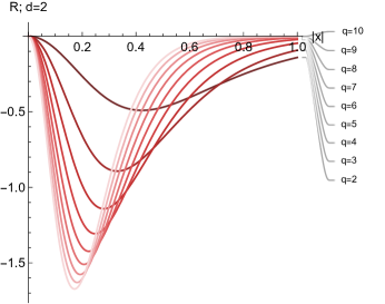
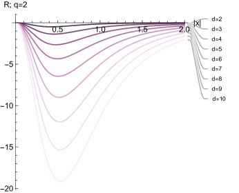
Figure C.1: Ricci curvature scalar $R$ (C.46) as a function of input modulus $\|\mathbf{x}\|$ for monomial activation function NNGPs of varying degree $q$ and input dimension $d$. At left, we show the effect of varying the degree $q$ (with lighter shades of red indicated higher degrees) for fixed dimension $d=2$. At right, we show the effect of varying the dimension $d$ (with lighter shades of purple indicating higher degrees) for fixed degree $q=2$. In all cases, the weight and bias variances are fixed to unity, i.e., $\sigma^{2}=\zeta^{2}=1$.

The Ricci curvature is somewhat more complicated. First, we can see that $R=0$ if $q=1$ or $d=1$, which we would expect. We can then restrict our attention to $d>1$ and $q>1$. If $\zeta=0$, $R=0$ if $d=2$ and $R<0$ for all $d>2$, but, unlike for the error function, $|R|$ is monotonically decreasing with $\|\mathbf{x}\|$. We now consider $\zeta>0$. By differentiation, we have

$$\frac{\partial R}{\partial(\sigma^{2}\|\mathbf{x}\|^{2})} \propto(d-2)(2q-1)^{2}q(\sigma^{2}\|\mathbf{x}\|^{2})^{3}+(2q-1)[(2q-1)d+6]\zeta^{2}(\sigma^{2}\|\mathbf{x}\|^{2})^{2}$$

$$\quad-[8+q(d-14)]\zeta^{4}(\sigma^{2}\|\mathbf{x}\|^{2})-(d+2)\zeta^{6},$$ (C.49)

where the implied constant of proportionality is strictly positive. This suggests that $R$ is non-monotonic, with an initial decrease followed by a gradual increase towards zero as $\|\mathbf{x}\|\to\infty$. We illustrate this behavior across degrees $q$ and input dimensions $d$ in Figure C.1. In $d=2$, we have the simplification that the equation $\partial R/\partial(\sigma^{2}\|\mathbf{x}\|^{2})=0$ is quadratic rather than cubic, and we find easily that $\partial R/\partial(\sigma^{2}\|\mathbf{x}\|^{2})<0$ if $\sigma^{2}\|\mathbf{x}\|^{2}<C$, $\partial R/\partial(\sigma^{2}\|\mathbf{x}\|^{2})=0$ if $\sigma^{2}\|\mathbf{x}\|^{2}=C$, and $\partial R/\partial(\sigma^{2}\|\mathbf{x}\|^{2})>0$ if $\sigma^{2}\|\mathbf{x}\|^{2}>C$, where the threshold value is determined by

$$[2q^{2}+q-1]C^{2}+(3q-2)\zeta^{2}C-\zeta^{4}=0,$$ (C.50)

hence

$$C=\frac{\sqrt{17q^{2}-8q}-3q+2}{2(2q^{2}+q-1)}\zeta^{2}.$$ (C.51)

For $q=2$, this gives $\sqrt{C}\simeq 0.42\zeta$, which is consistent with our numerical results in Figure 1.

Appendix D Comparing the shallow Neural Tangent Kernel to the NNGP

In this section, we compare the shallow NTK to the shallow NNGP. For a shallow network

$$f(\mathbf{x})=\frac{1}{\sqrt{n}}\sum_{j=1}^{n}v_{j}\phi(\mathbf{w}_{j}\cdot\mathbf{x}+b_{j}),$$ (D.1)

the empirical NTK is

$$\Theta_{e}(\mathbf{x},\mathbf{y}) =\frac{1}{n}\sum_{j=1}^{n}\phi(\mathbf{w}_{j}\cdot\mathbf{x}+b_{j})\phi(\mathbf{w}_{j}\cdot\mathbf{y}+b_{j})$$

$$\quad+\frac{1}{n}\sum_{j=1}^{n}v_{j}^{2}\phi^{\prime}(\mathbf{w}_{j}\cdot\mathbf{x}+b_{j})\phi^{\prime}(\mathbf{w}_{j}\cdot\mathbf{y}+b_{j})(1+\mathbf{x}\cdot\mathbf{y})$$ (D.2)

and, taking $\mathbf{w}\sim\mathcal{N}(\mathbf{0},\sigma^{2}\mathbf{I}_{d})$, $b\sim\mathcal{N}(0,\zeta^{2})$, and $\mathbf{v}\sim\mathcal{N}(\mathbf{0},\xi^{2}\mathbf{I}_{n})$, the infinite-width NTK is

$$\Theta(\mathbf{x},\mathbf{y}) =\mathbb{E}[\phi(\mathbf{w}\cdot\mathbf{x}+b)\phi(\mathbf{w}\cdot\mathbf{y}+b)]+\xi^{2}\mathbb{E}[\phi^{\prime}(\mathbf{w}\cdot\mathbf{x}+b)\phi^{\prime}(\mathbf{w}\cdot\mathbf{y}+b)](1+\mathbf{x}\cdot\mathbf{y})$$ (D.3)

where the remaining expectations are taken over $\mathbf{w}$ and $b$.

Writing $z\equiv\mathbf{w}\cdot\mathbf{x}+b$, we have

$$\frac{\partial^{2}}{\partial x_{\mu}\partial x_{\nu}}\Theta(\mathbf{x},\mathbf{x})$$

$$=\frac{\partial^{2}}{\partial x_{\mu}\partial x_{\nu}}\bigg{[}\mathbb{E}[\phi(z)^{2}]+\xi^{2}\mathbb{E}[\phi^{\prime}(z)^{2}](1+\|\mathbf{x}\|^{2})\bigg{]}$$ (D.4)

$$=\frac{\partial}{\partial x_{\mu}}\bigg{[}2\mathbb{E}[\phi(z)\phi^{\prime}(z)w_{\nu}]+2\xi^{2}\mathbb{E}[\phi^{\prime}(z)\phi^{\prime\prime}(z)w_{\nu}](1+\|\mathbf{x}\|^{2})+2\xi^{2}\mathbb{E}[\phi^{\prime}(z)^{2}]x_{\nu}\bigg{]}$$ (D.5)

$$=2\mathbb{E}[\{\phi^{\prime}(z)^{2}+\phi(z)\phi^{\prime\prime}(z)\}w_{\mu}w_{\nu}]+2\xi^{2}\mathbb{E}[\{\phi^{\prime\prime}(z)^{2}+\phi^{\prime}(z)\phi^{\prime\prime\prime}(z)\}w_{\mu}w_{\nu}](1+\|\mathbf{x}\|^{2})$$

$$\quad+4\xi^{2}\mathbb{E}[\phi^{\prime}(z)\phi^{\prime\prime}(z)w_{\nu}]x_{\mu}+4\xi^{2}\mathbb{E}[\phi^{\prime}(z)\phi^{\prime\prime}(z)w_{\mu}]x_{\nu}+2\xi^{2}\mathbb{E}[\phi^{\prime}(z)^{2}]\delta_{\mu\nu}$$ (D.6)

while

$$\frac{\partial^{2}}{\partial y_{\mu}\partial y_{\nu}}\Theta(\mathbf{x},\mathbf{y})$$

$$=\frac{\partial^{2}}{\partial y_{\mu}\partial y_{\nu}}\bigg{[}\mathbb{E}[\phi(\mathbf{w}\cdot\mathbf{x}+b)\phi(\mathbf{w}\cdot\mathbf{y}+b)]+\xi^{2}\mathbb{E}[\phi^{\prime}(\mathbf{w}\cdot\mathbf{x}+b)\phi^{\prime}(\mathbf{w}\cdot\mathbf{y}+b)](1+\mathbf{x}\cdot\mathbf{y})\bigg{]}$$ (D.7)

$$=\frac{\partial}{\partial y_{\mu}}\bigg{[}\mathbb{E}[\phi(\mathbf{w}\cdot\mathbf{x}+b)\phi^{\prime}(\mathbf{w}\cdot\mathbf{y}+b)w_{\nu}]+\xi^{2}\mathbb{E}[\phi^{\prime}(\mathbf{w}\cdot\mathbf{x}+b)\phi^{\prime\prime}(\mathbf{w}\cdot\mathbf{y}+b)w_{\nu}](1+\mathbf{x}\cdot\mathbf{y})$$

$$\qquad\qquad+\xi^{2}\mathbb{E}[\phi^{\prime}(\mathbf{w}\cdot\mathbf{x}+b)\phi^{\prime}(\mathbf{w}\cdot\mathbf{y}+b)]x_{\nu}\bigg{]}$$ (D.8)

$$=\mathbb{E}[\phi(\mathbf{w}\cdot\mathbf{x}+b)\phi^{\prime\prime}(\mathbf{w}\cdot\mathbf{y}+b)w_{\mu}w_{\nu}]+\xi^{2}\mathbb{E}[\phi^{\prime}(\mathbf{w}\cdot\mathbf{x}+b)\phi^{\prime\prime\prime}(\mathbf{w}\cdot\mathbf{y}+b)w_{\mu}w_{\nu}](1+\mathbf{x}\cdot\mathbf{y})$$

$$\quad+\xi^{2}\mathbb{E}[\phi^{\prime}(\mathbf{w}\cdot\mathbf{x}+b)\phi^{\prime\prime}(\mathbf{w}\cdot\mathbf{y}+b)w_{\nu}]x_{\mu}+\xi^{2}\mathbb{E}[\phi^{\prime}(\mathbf{w}\cdot\mathbf{x}+b)\phi^{\prime\prime}(\mathbf{w}\cdot\mathbf{y}+b)w_{\mu}]x_{\nu}$$ (D.9)

hence

$$\left[\frac{\partial^{2}}{\partial y_{\mu}\partial y_{\nu}}\Theta(\mathbf{x},\mathbf{y})\right]_{\mathbf{y}=\mathbf{x}} =\mathbb{E}[\phi(z)\phi^{\prime\prime}(z)w_{\mu}w_{\nu}]+\xi^{2}\mathbb{E}[\phi^{\prime}(z)\phi^{\prime\prime\prime}(z)w_{\mu}w_{\nu}](1+\|\mathbf{x}\|^{2})$$

$$\qquad\qquad+\xi^{2}\mathbb{E}[\phi^{\prime}(z)\phi^{\prime\prime}(z)w_{\nu}]x_{\mu}+\xi^{2}\mathbb{E}[\phi^{\prime}(z)\phi^{\prime\prime}(z)w_{\mu}]x_{\mu}.$$ (D.10)

Therefore, we have

$$g_{\mu\nu} =\frac{1}{2}\frac{\partial^{2}}{\partial x_{\mu}\partial x_{\nu}}\Theta(\mathbf{x},\mathbf{x})-\left[\frac{\partial^{2}}{\partial y_{\mu}\partial y_{\nu}}\Theta(\mathbf{x},\mathbf{y})\right]_{\mathbf{y}=\mathbf{x}}$$ (D.11)

$$=\mathbb{E}[\phi^{\prime}(z)^{2}w_{\mu}w_{\nu}]+\xi^{2}\mathbb{E}[\phi^{\prime\prime}(z)^{2}w_{\mu}w_{\nu}](1+\|\mathbf{x}\|^{2})$$

$$\quad+\xi^{2}\mathbb{E}[\phi^{\prime}(z)\phi^{\prime\prime}(z)w_{\nu}]x_{\mu}+\xi^{2}\mathbb{E}[\phi^{\prime}(z)\phi^{\prime\prime}(z)w_{\mu}]x_{\nu}+\xi^{2}\mathbb{E}[\phi^{\prime}(z)^{2}]\delta_{\mu\nu}.$$ (D.12)

By Stein’s lemma, as in the NNGP case,

$$\mathbb{E}[\phi^{\prime}(z)^{2}w_{\mu}w_{\nu}] =\sigma^{2}\mathbb{E}[\phi^{\prime}(z)^{2}]\delta_{\mu\nu}+2\sigma^{4}\mathbb{E}[\phi^{\prime\prime}(z)^{2}+\phi^{\prime}(z)\phi^{\prime\prime\prime}(z)]x_{\mu}x_{\nu}$$ (D.13)

and

$$\mathbb{E}[\phi^{\prime\prime}(z)^{2}w_{\mu}w_{\nu}] =\sigma^{2}\mathbb{E}[\phi^{\prime\prime}(z)^{2}]\delta_{\mu\nu}+2\sigma^{4}\mathbb{E}[\phi^{\prime\prime\prime}(z)^{2}+\phi^{\prime\prime}(z)\phi^{\prime\prime\prime\prime}(z)]x_{\mu}x_{\nu}$$ (D.14)

while

$$\mathbb{E}[\phi^{\prime}(z)\phi^{\prime\prime}(z)w_{\nu}] =\sigma^{2}\mathbb{E}[\phi^{\prime\prime}(z)^{2}+\phi^{\prime}(z)\phi^{\prime\prime\prime}(z)]x_{\nu},$$ (D.15)

and therefore

$$g_{\mu\nu}$$

$$=\mathbb{E}[\phi^{\prime}(z)^{2}w_{\mu}w_{\nu}]+\xi^{2}\mathbb{E}[\phi^{\prime\prime}(z)^{2}w_{\mu}w_{\nu}](1+\|\mathbf{x}\|^{2})$$

$$\quad+\xi^{2}\mathbb{E}[\phi^{\prime}(z)\phi^{\prime\prime}(z)w_{\nu}]x_{\mu}+\xi^{2}\mathbb{E}[\phi^{\prime}(z)\phi^{\prime\prime}(z)w_{\mu}]x_{\nu}+\xi^{2}\mathbb{E}[\phi^{\prime}(z)^{2}]\delta_{\mu\nu}$$ (D.16)

$$=\bigg{[}(\sigma^{2}+\xi^{2})\mathbb{E}[\phi^{\prime}(z)^{2}]+\sigma^{2}\xi^{2}\mathbb{E}[\phi^{\prime\prime}(z)^{2}](1+\|\mathbf{x}\|^{2})\bigg{]}\delta_{\mu\nu}$$

$$\quad+2\sigma^{2}\bigg{[}(\sigma^{2}+\xi^{2})\mathbb{E}[\phi^{\prime\prime}(z)^{2}+\phi^{\prime}(z)\phi^{\prime\prime\prime}(z)]+\sigma^{2}\xi^{2}\mathbb{E}[\phi^{\prime\prime\prime}(z)^{2}+\phi^{\prime\prime}(z)\phi^{\prime\prime\prime\prime}(z)](1+\|\mathbf{x}\|^{2})\bigg{]}x_{\mu}x_{\nu}$$ (D.17)

This metric is not quite of the special form of the NNGP metric, as

$$\frac{d}{d\|\mathbf{x}\|^{2}}\bigg{[}(\sigma^{2}+\xi^{2})\mathbb{E}[\phi^{\prime}(z)^{2}]+\sigma^{2}\xi^{2}\mathbb{E}[\phi^{\prime\prime}(z)^{2}](1+\|\mathbf{x}\|^{2})\bigg{]}$$

$$\quad=\sigma^{2}\bigg{[}(\sigma^{2}+\xi^{2})\mathbb{E}[\phi^{\prime\prime}(z)^{2}+\phi^{\prime}(z)\phi^{\prime\prime\prime}(z)]+\sigma^{2}\xi^{2}\mathbb{E}[\phi^{\prime\prime\prime}(z)^{2}+\phi^{\prime\prime}(z)\phi^{\prime\prime\prime\prime}(z)](1+\|\mathbf{x}\|^{2})\bigg{]}$$

$$\qquad+\sigma^{2}\xi^{2}\mathbb{E}[\phi^{\prime\prime}(z)^{2}]$$ (D.18)

by Price’s theorem, hence we have

$$g_{\mu\nu}=\omega(\|\mathbf{x}\|^{2})\delta_{\mu\nu}+2\left[\omega^{\prime}(\|\mathbf{x}\|^{2})-\sigma^{2}\xi^{2}\mathbb{E}[\phi^{\prime\prime}(z)^{2}]\right]x_{\mu}x_{\nu}$$ (D.19)

for

$$\omega(\|\mathbf{x}\|^{2})=(\sigma^{2}+\xi^{2})\mathbb{E}[\phi^{\prime}(z)^{2}]+\sigma^{2}\xi^{2}\mathbb{E}[\phi^{\prime\prime}(z)^{2}](1+\|\mathbf{x}\|^{2})$$ (D.20)

Even though the geometric quantities associated with this metric are not as easy to compute as those for the NNGP kernel, we can see that it shares similar symmetries. In particular, it still takes the form of a projection, and the volume element will depend on the input only through its norm.

Appendix E Perturbative finite-width corrections in shallow Bayesian neural networks

In this section, we describe how one may compute perturbative corrections to geometric quantities in shallow Bayesian neural networks at large but finite width (Zavatone-Veth et al., 2021; Roberts et al., 2022). For simplicity, we will focus on corrections to the volume element. We will not go through the straightforward but tedious exercise of computing perturbative corrections to the Riemann tensor and Ricci scalar (Misner et al., 2017). We will follow the notation and formalism of Zavatone-Veth et al. (2021); we could equivalently use the formalism of Roberts et al. (2022).

We begin by considering the effect of a general perturbation to the metric that preserves the index-permutation symmetry of its derivatives. We write the metric tensor as $g_{\mu\nu}=\bar{g}_{\mu\nu}+h_{\mu\nu}$ for some background metric $\bar{g}_{\mu\nu}$ and a small perturbation $h_{\mu\nu}$. By Jacobi’s formula for the variation of a determinant, we have

$$\det g=[1+\bar{g}^{\mu\nu}h_{\mu\nu}+\mathcal{O}(h^{2})]\det\bar{g},$$ (E.1)

hence the volume element expands as

$$\sqrt{\det g}=\left[1+\frac{1}{2}\bar{g}^{\mu\nu}h_{\mu\nu}+\mathcal{O}(h^{2})\right]\sqrt{\det\bar{g}}.$$ (E.2)

E.1 Metric perturbations for a wide Bayesian neural network

We now consider the concrete setting of a Bayesian neural network with a single hidden layer of large but finite width $n$ and $m$-dimensional output,

$$\mathbf{f}(\mathbf{x};\mathbf{W},\mathbf{V})=\frac{1}{\sqrt{n}}\sum_{i=1}^{n}\mathbf{v}_{i}\phi(\mathbf{w}_{i}\cdot\mathbf{x}).$$ (E.3)

We fix isotropic standard Gaussian priors over the weights, and, for a training dataset $\{(\mathbf{x}_{a},\mathbf{y}_{a})\}_{a=1}^{p}$ of $p$ examples, choose an isotropic Gaussian likelihood of inverse variance $\beta$:

$$p(\{(\mathbf{x}_{a},\mathbf{y}_{a})\}_{a=1}^{p}\,|\,\mathbf{W},\mathbf{V})\propto\exp\left(-\frac{\beta}{2}\sum_{a=1}^{p}\|\mathbf{f}(\mathbf{x}_{a};\mathbf{W},\mathbf{V})-\mathbf{y}_{a}\|_{2}^{2}\right).$$ (E.4)

We denote expectation with respect to the resulting Bayes posterior by $\langle\cdot\rangle$. Our choice of unit-variance priors is made without much loss of generality, as changing the prior variance does not change the qualitative structure of perturbative feature learning (Zavatone-Veth et al., 2021).

Using the nomenclature of Zavatone-Veth et al. (2021) and Roberts et al. (2022), the metric

$$g_{\mu\nu}=\frac{1}{n}\sum_{i=1}^{n}\phi^{\prime}(\mathbf{w}_{j}\cdot\mathbf{x})^{2}w_{i\mu}w_{i\nu}$$ (E.5)

is a hidden layer observable, with infinite-width limit given by the metric $\bar{g}_{\mu\nu}$ associated with the NNGP kernel of the network,

$$\bar{g}_{\mu\nu}=\mathbb{E}_{\mathcal{W}}g_{\mu\nu}=\mathbb{E}_{\mathbf{w}\sim\mathcal{N}(\mathbf{0},\mathbf{I}_{d})}[\phi^{\prime}(\mathbf{w}\cdot\mathbf{x})^{2}w_{\mu}w_{\nu}]$$ (E.6)

where $\mathbb{E}_{\mathcal{W}}$ denotes expectation with respect to the prior distribution. Then, we may apply the result of Zavatone-Veth et al. (2021) for the perturbative expansion of posterior moments of $g_{\mu\nu}$ at large width. To state the result, we must first introduce some notation. Let

$$k(\mathbf{x},\mathbf{y})=\frac{1}{n}\sum_{i=1}^{n}\phi(\mathbf{w}_{i}\cdot\mathbf{x})\phi(\mathbf{w}_{i}\cdot\mathbf{y})$$ (E.7)

be the hidden layer kernel, and

$$\bar{k}(\mathbf{x},\mathbf{y})=\mathbb{E}_{\mathbf{w}\sim\mathcal{N}(\mathbf{0},\mathbf{I}_{d})}[\phi(\mathbf{w}\cdot\mathbf{x})\phi(\mathbf{w}\cdot\mathbf{y})]$$ (E.8)

be its infinite-width limit, i.e., the NNGP kernel. Then, define the $p\times p$ matrix

$$\bm{\Psi}\equiv\bm{\Gamma}^{-1}\mathbf{G}_{yy}\bm{\Gamma}^{-1}-\bm{\Gamma}^{-1},$$ (E.9)

where the $p\times p$ matrix $\bm{\Gamma}$ is defined as

$$\Gamma_{ab}\equiv\bar{k}(\mathbf{x}_{a},\mathbf{x}_{b})+\beta^{-1}\delta_{ab}$$ (E.10)

and $\mathbf{G}_{yy}$ is the normalized target Gram matrix,

$$(G_{yy})_{ab}=\frac{1}{m}\mathbf{y}_{a}\cdot\mathbf{y}_{b}.$$ (E.11)

Then, the result of Zavatone-Veth et al. (2021) yields the perturbative expansion

$$\langle g_{\mu\nu}\rangle =\bar{g}_{\mu\nu}+\frac{1}{2}m\sum_{a,b=1}^{p}\Psi_{ab}\operatorname{cov}_{\mathbf{w}}[k(\mathbf{x}_{a},\mathbf{x}_{b}),g_{\mu\nu}]+\mathcal{O}\left(\frac{1}{n^{2}}\right)$$ (E.12)

where the required posterior covariance can be explicitly expressed as

$$n\operatorname{cov}_{\mathbf{w}}[k(\mathbf{x}_{a},\mathbf{x}_{b}),g_{\mu\nu}] =\mathbb{E}_{\mathbf{w}\sim\mathcal{N}(\mathbf{0},\mathbf{I}_{d})}[\phi(z_{a})\phi(z_{b})\phi^{\prime}(z)^{2}w_{\mu}w_{\nu}]-\bar{k}(\mathbf{x}_{a},\mathbf{x}_{b})\bar{g}_{\mu\nu},$$ (E.13)

where we write $z_{a}\equiv\mathbf{w}\cdot\mathbf{x}_{a}$ and $z\equiv\mathbf{w}\cdot\mathbf{x}$. This formula alternatively follows from applying the result of Zavatone-Veth et al. (2021) for the asymptotics of the mean kernel, and then using the formula for the metric in terms of derivatives of the kernel (Burges, 1999).

In general, this expression is somewhat unwieldy, and the integrals are challenging to evaluate in closed form. However, the situation simplifies dramatically if we train with only a single datapoint, and focus on the zero-temperature limit $\beta\to\infty$. In this case, we can set $m=1$ with very little loss of generality. We then have the simplified expression

$$\langle g_{\mu\nu}\rangle =\bar{g}_{\mu\nu}+\frac{1}{2}\left(\frac{y_{a}^{2}}{\mathbb{E}_{\mathbf{w}}[\phi(z_{a})^{2}]}-1\right)\frac{\operatorname{cov}_{\mathbf{w}}[k(\mathbf{x}_{a},\mathbf{x}_{a}),g_{\mu\nu}]}{\mathbb{E}_{\mathbf{w}}[\phi(z_{a})^{2}]}+\mathcal{O}\left(\frac{1}{n^{2}}\right)$$ (E.14)

hence, to the order of interest, the volume element expands as

$$\frac{\langle\sqrt{\det g}\rangle}{\sqrt{\det\bar{g}}} =\frac{\sqrt{\det\langle g\rangle}}{\sqrt{\det\bar{g}}}+\mathcal{O}\left(\frac{1}{n^{2}}\right)$$ (E.15)

$$=1+\frac{1}{4n}\left(\frac{y_{a}^{2}}{\mathbb{E}_{\mathbf{w}}[\phi(z_{a})^{2}]}-1\right)(\chi-d)+\mathcal{O}\left(\frac{1}{n^{2}}\right),$$ (E.16)

where we have defined

$$\chi\equiv\frac{\bar{g}^{\mu\nu}\mathbb{E}_{\mathbf{w}}[\phi(z_{a})^{2}\phi^{\prime}(z)^{2}w_{\mu}w_{\nu}]}{{\mathbb{E}_{\mathbf{w}}[\phi(z_{a})^{2}]}}$$ (E.17)

and used the facts that $\bar{g}^{\mu\nu}\bar{g}_{\mu\nu}=d$ and $\bar{k}(\mathbf{x}_{a},\mathbf{x}_{a})=\mathbb{E}_{\mathbf{w}}[\phi(z_{a})^{2}]$.

From Appendix C, we know that

$$\bar{g}^{\mu\nu}=e^{-\Omega}\left[\delta_{\mu\nu}-\frac{2\Omega^{\prime}}{1+2\|\mathbf{x}\|^{2}\Omega^{\prime}}x_{\mu}x_{\nu}\right]$$ (E.18)

for $\Omega(\|\mathbf{x}\|^{2})$ defined by

$$\exp\Omega(\|\mathbf{x}\|^{2})\equiv\mathbb{E}_{\mathbf{w}}[\phi^{\prime}(z)^{2}],$$ (E.19)

so we have

$$\chi =\frac{1}{e^{\Omega}\mathbb{E}_{\mathbf{w}}[\phi(z_{a})^{2}]}\mathbb{E}_{\mathbf{w}}[\phi(z_{a})^{2}\phi^{\prime}(z)^{2}w_{\mu}w_{\nu}\delta_{\mu\nu}]$$

$$\quad-\frac{1}{e^{\Omega}\mathbb{E}_{\mathbf{w}}[\phi(z_{a})^{2}]}\frac{2\Omega^{\prime}}{1+2\|\mathbf{x}\|^{2}\Omega^{\prime}}\mathbb{E}_{\mathbf{w}}[\phi(z_{a})^{2}\phi^{\prime}(z)^{2}z^{2}]$$ (E.20)

Using Stein’s lemma, we have

$$\mathbb{E}_{\mathbf{w}}[\phi(z_{a})^{2}\phi^{\prime}(z)^{2}w_{\mu}w_{\nu}\delta_{\mu\nu}] =d\mathbb{E}_{\mathbf{w}}[\phi(z_{a})^{2}\phi^{\prime}(z)^{2}]$$

$$\quad+2\mathbb{E}_{\mathbf{w}}[\phi(z_{a})\phi^{\prime}(z_{a})z_{a}\phi^{\prime}(z)^{2}+\phi(z_{a})^{2}\phi^{\prime}(z)\phi^{\prime\prime}(z)z].$$ (E.21)

E.2 A tractable example: monomial activation functions

We now specialize to the case of $\phi(x)=x^{q}/\sqrt{(2q-1)!!}$, in which all of the required expectations can be evaluated analytically. In this case, we have the explicit formula

$$\exp\Omega(\|\mathbf{x}\|^{2})=\mathbb{E}[\phi^{\prime}(z)^{2}]=\frac{q^{2}}{2q-1}\|\mathbf{x}\|^{2q-2}.$$ (E.22)

Noting that

$$\mathbb{E}_{\mathbf{w}}[\phi(z_{a})\phi^{\prime}(z_{a})z_{a}\phi^{\prime}(z)^{2}]=q\mathbb{E}_{\mathbf{w}}[\phi(z_{a})^{2}\phi^{\prime}(z)^{2}]$$ (E.23)

and

$$\mathbb{E}_{\mathbf{w}}[\phi(z_{a})^{2}\phi^{\prime}(z)\phi^{\prime\prime}(z)z]=(q-1)\mathbb{E}_{\mathbf{w}}[\phi(z_{a})^{2}\phi^{\prime}(z)^{2}],$$ (E.24)

we have

$$\mathbb{E}_{\mathbf{w}}[\phi(z_{a})^{2}\phi^{\prime}(z)^{2}w_{\mu}w_{\nu}\delta_{\mu\nu}] =[d+2(2q-1)]\mathbb{E}_{\mathbf{w}}[\phi(z_{a})^{2}\phi^{\prime}(z)^{2}]$$ (E.25)

$$=\frac{q^{2}}{[(2q-1)!!]^{2}}[d+2(2q-1)]\mathbb{E}_{\mathbf{w}}[z_{a}^{2q}z^{2q-2}]$$ (E.26)

and, similarly,

$$\mathbb{E}_{\mathbf{w}}[\phi(z_{a})^{2}\phi^{\prime}(z)^{2}z^{2}] =\frac{q^{2}}{[(2q-1)!!]^{2}}\mathbb{E}_{\mathbf{w}}[z_{a}^{2q}z^{2q}].$$ (E.27)

Then, using the formula for $e^{\Omega}$ and the fact that $\mathbb{E}_{\mathbf{w}}[\phi(z_{a})^{2}]=\|\mathbf{x}_{a}\|^{2q}$, we have

$$\chi(\rho^{2}) =\frac{(2q-1)}{[(2q-1)!!]^{2}}[d+2(2q-1)]\mathbb{E}_{\mathbf{w}}[u_{a}^{2q}u^{2q-2}]-\frac{2(q-1)}{[(2q-1)!!]^{2}}\mathbb{E}_{\mathbf{w}}[u_{a}^{2q}u^{2q}]$$ (E.28)

where we have let

$$\begin{pmatrix}u_{a}\\ u\end{pmatrix}=\begin{pmatrix}z_{a}/\|\mathbf{x}_{a}\|\\ z/\|\mathbf{x}\|\end{pmatrix}\sim\mathcal{N}\left(\begin{pmatrix}0\\ 0\end{pmatrix},\begin{pmatrix}1&\rho\\ \rho&1\end{pmatrix}\right)$$ (E.29)

for

$$\rho=\frac{\mathbf{x}_{a}\cdot\mathbf{x}}{\|\mathbf{x}_{a}\|\|\mathbf{x}\|}.$$ (E.30)

In general, we have

$$\frac{1}{[(2q-1)!!]^{2}}\mathbb{E}_{\mathbf{w}}[u_{a}^{2q}u^{2q}] ={{}_{2}F_{1}}\left(-q,-q;\frac{1}{2};\rho^{2}\right)$$ (E.31)

and

$$\frac{2q-1}{[(2q-1)!!]^{2}}\mathbb{E}_{\mathbf{w}}[u_{a}^{2q}u^{2q-2}] ={{}_{2}F_{1}}\left(1-q,-q;\frac{1}{2};\rho^{2}\right)$$ (E.32)

in terms of the Gauss hypergeometric function (DLMF, ). Thus, we have

$$\chi(\rho^{2}) =[d+2(2q-1)]{{}_{2}F_{1}}\left(1-q,-q;\frac{1}{2};\rho^{2}\right)-2(q-1){{}_{2}F_{1}}\left(-q,-q;\frac{1}{2};\rho^{2}\right).$$ (E.33)

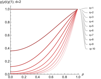
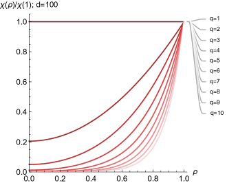
Figure E.1: Normalized perturbative expansion factor $\chi(\rho^{2})/\chi(\rho=1)$ as a function of overlap $\rho$ for Bayesian MLPs with monomial activation functions of varying degree $q$ (with larger $q$ indicated by lighter shades of red) in $d=2$ (left) and $d=100$ (right). See main text for details.

Each of these hypergeometric functions is a polynomial with all-positive coefficients in $\rho^{2}$, and both evaluate to unity when $\rho=0$ (DLMF, ). At small order, we have

$$\chi\bigg{|}_{q=1}-d =2$$ (E.34)

for linear networks and

$$\chi\bigg{|}_{q=2}-d =4\left(\frac{4}{3}\rho^{4}+(d+2)\rho^{2}+1\right)$$ (E.35)

for quadratic networks. Then, at $\rho=0$, one can easily show that

$$\chi(\rho=0)=d+2q$$ (E.36)

and, as $\rho$ increases from zero to one, $\chi$ increases monotonically (for all $q>1$; for $q=1$ it is constant) to

$$\lim_{\rho\uparrow 1}\chi(1)=\frac{(2(2q-1)-1)!!}{[(2q-1)!!]^{2}}[(2q-1)d+2q]$$ (E.37)

using formulas for hypergeometric functions of unit argument (DLMF, ). Thus, $\chi(\rho^{2})-d$ is strictly positive for all $\rho$, $d$, and $q$. We plot $\chi(\rho^{2})/\chi(1)$ for varying degrees in $d=2$ and $d=100$ in Figure E.1 to illustrate the increasing relative separation between $\rho(0)$ and $\rho(1)$ with increasing $d$ and $q$.

Collecting our results, the general expansion (E.15) for the magnification factor simplifies to

$$\frac{\langle\sqrt{\det g}\rangle}{\sqrt{\det\bar{g}}} =1+\frac{1}{4n}\left(\frac{y_{a}^{2}}{\|\mathbf{x}_{a}\|^{2q}}-1\right)(\chi(\rho^{2})-d)+\mathcal{O}\left(\frac{1}{n^{2}}\right).$$ (E.38)

As $\chi(\rho^{2})>d$ for all $\rho$, we can see that if $\|\mathbf{x}_{a}\|^{2q}>y_{a}^{2}$, the leading correction compresses areas, while if $\|\mathbf{x}_{a}\|^{2q}<y_{a}^{2}$, it expands them. As $\chi(\rho^{2})-d$ is monotonically increasing in the overlap $\rho=\frac{\mathbf{x}_{a}\cdot\mathbf{x}}{\|\mathbf{x}_{a}\|\|\mathbf{x}\|}$, the expansion or contraction is minimal for points orthogonal to the training example $\mathbf{x}_{a}$, and maximal for points parallel to the training example.

We remark that the dependence on the scale of $\mathbf{x}_{a}$ relative to $y_{a}$ parallels the conditions under which generalization error decreases with increasing width in deep linear networks (Zavatone-Veth et al., 2022b, 2021): with unit-variance priors, increasing width is beneficial if

$$\frac{y_{a}^{2}}{\|\mathbf{x}_{a}\|^{2}}>1$$ (E.39)

as shown in Zavatone-Veth et al. (2021). This is a simple consequence of the fact that the sign of the leading perturbative correction is determined by the same quantity. We note that, under the prior, as $\mathbf{v}\sim\mathcal{N}(\mathbf{0},\mathbf{I}_{n})$,

$$\mathbb{E}_{\mathbf{w},\mathbf{v}}[f(\mathbf{x}_{a})^{2}] =\mathbb{E}_{\mathbf{w}}[\phi(z_{a})^{2}]$$ (E.40)

$$=\|\mathbf{x}_{a}\|^{2q},$$ (E.41)

so this is a comparison of the variance of the function output under the prior to the target magnitude.

As an example, consider training a network on one point of the XOR task: $(1,1)\mapsto 0$. In this case, $\|\mathbf{x}_{a}\|^{2q}>y_{a}^{2}$, so the volume element will be contracted everywhere, maximally along the line $x_{1}=x_{2}$ and minimally orthogonal to this line.

Appendix F The geometry of kernel learning algorithms

In this appendix, we give a detailed analysis of the changes in representational geometry resulting from the original kernel learning algorithm of Amari and Wu (1999), as well as kernel learning algorithms recently proposed by Radhakrishnan et al. (2022) and Simon et al. (2023).

F.1 The supervised kernel learning algorithm of Amari and Wu

We begin with a detailed, pedagogical analysis of the kernel learning algorithm proposed by Amari and Wu that we mentioned in §3. This analysis follows that in their original paper, with some additional detail. For some base kernel $k(\mathbf{x},\mathbf{y})$, they fit an SVM to obtain a set of support vectors $\textrm{SV}(k)$ for $k$. Then, fixing a bandwidth parameter $\tau>0$, they define a new kernel

$$\tilde{k}(\mathbf{x},\mathbf{y})=h(\mathbf{x})h(\mathbf{y})k(\mathbf{x},\mathbf{y})$$ (F.1)

for

$$h(\mathbf{x})=\sum_{\mathbf{v}\in\textrm{SV}(k)}\exp\left[-\frac{\|\mathbf{x}-\mathbf{v}\|^{2}}{2\tau^{2}}\right],$$ (F.2)

and fit a new SVM with the modified kernel $\tilde{k}$. Under this transformation, the induced metric changes as

$$\tilde{g}_{\mu\nu}=h(\mathbf{x})^{2}g_{\mu\nu}+\frac{\partial h(\mathbf{x})}{\partial x_{\mu}}\frac{\partial h(\mathbf{x})}{\partial x_{\nu}}k(\mathbf{x},\mathbf{x})+h(\mathbf{x})\left[\frac{\partial h(\mathbf{x})}{\partial x_{\mu}}\frac{\partial k(\mathbf{x},\mathbf{y})}{\partial y_{\nu}}+\frac{\partial h(\mathbf{x})}{\partial x_{\nu}}\frac{\partial k(\mathbf{x},\mathbf{y})}{\partial y_{\mu}}\right]_{\mathbf{y}=\mathbf{x}},$$ (F.3)

where $g_{\mu\nu}$ is the metric induced by $k$. In their original work, Amari and Wu (1999) focus on a single iteration of this algorithm, though they consider multiple updates in later works (Wu and Amari, 2002; Williams et al., 2007).

Here, we will follow their original paper, and consider the effect of a single update starting from the radial basis function kernel

$$k(\mathbf{x},\mathbf{y})=\exp\left[-\frac{1}{2\sigma^{2}}\|\mathbf{x}-\mathbf{y}\|^{2}\right]$$ (F.4)

of bandwidth $\sigma^{2}$ on the induced geometry. For the RBF kernel, we of course have

$$\frac{\partial k(\mathbf{x},\mathbf{y})}{\partial y_{\mu}}\bigg{|}_{\mathbf{y}=\mathbf{x}} =-\frac{1}{\sigma^{2}}k(\mathbf{x},\mathbf{y})(x_{\mu}-y_{\mu})\bigg{|}_{\mathbf{y}=\mathbf{x}}=0,$$ (F.5)

hence the third term in (F.3) vanishes and the first update to the metric is rank-1. Moreover, the metric induced by the radial basis function kernel is

$$g_{\mu\nu}=\frac{1}{\sigma^{2}}\delta_{\mu\nu}$$ (F.6)

as shown by Amari and Wu (1999) and by Burges (1999), which leaves us with

$$\tilde{g}_{\mu\nu}=\frac{h(\mathbf{x})^{2}}{\sigma^{2}}\delta_{\mu\nu}+\frac{\partial h(\mathbf{x})}{\partial x_{\mu}}\frac{\partial h(\mathbf{x})}{\partial x_{\nu}}$$ (F.7)

as $k(\mathbf{x},\mathbf{x})=1$. Now, by the matrix determinant lemma, we have

$$\det\tilde{g} =\left(\frac{h(\mathbf{x})^{2}}{\sigma^{2}}\right)^{d}\left(1+\frac{\sigma^{2}}{h(\mathbf{x})^{2}}\frac{\partial h(\mathbf{x})}{\partial x_{\mu}}\frac{\partial h(\mathbf{x})}{\partial x_{\mu}}\right).$$ (F.8)

As

$$\frac{\partial h(\mathbf{x})}{\partial x_{\mu}}=\frac{1}{\tau^{2}}\sum_{\mathbf{v}\in\textrm{SV}(k)}\exp\left[-\frac{\|\mathbf{x}-\mathbf{v}\|^{2}}{2\tau^{2}}\right](v_{\mu}-x_{\mu}),$$ (F.9)

we will therefore have contributions of the volume element (or rather to its square) from different subsets of the support vectors. In their analysis, Amari and Wu (1999) focus on the case in which the support vectors are well-separated, and the bandwidth is small enough such that one can neglect the influence of all but one support vector on the metric. Then, locally, one has only a single Gaussian bump to contend with.

F.2 The supervised kernel learning algorithm of Radhakrishnan et al.

We now discuss the method for iterative supervised kernel learning proposed by Radhakrishnan et al. (2022). Their method starts with a translation-invariant kernel of the general form

$$k_{\mathbf{M}}(\mathbf{x},\mathbf{y})=h(\|\mathbf{x}-\mathbf{y}\|_{\mathbf{M}}^{2}),$$ (F.10)

where $h:\mathbb{R}_{\geq 0}\to\mathbb{R}_{\geq 0}$ is a suitably smooth scalar function and

$$\|\mathbf{x}-\mathbf{y}\|_{\mathbf{M}}^{2}=(\mathbf{x}-\mathbf{y})^{\top}\mathbf{M}(\mathbf{x}-\mathbf{y})$$ (F.11)

is the squared Mahalanobis distance between $\mathbf{x}$ and $\mathbf{y}$ for a constant positive-semidefinite symmetric matrix $\mathbf{M}$.

Then, for a dataset $\{(\mathbf{x}_{a},y_{a})\}_{a=1}^{p}$, they initialize $\mathbf{M}=\mathbf{I}_{d}$, fit a kernel machine

$$f_{\mathbf{M}}(\mathbf{x})=\sum_{a=1}^{p}y_{a}(\mathbf{K}_{\mathbf{M}}^{-1})_{ab}k_{\mathbf{M}}(\mathbf{x}_{b},\mathbf{x})$$ (F.12)

for $(\mathbf{K}_{\mathbf{M}})_{ab}=k_{\mathbf{M}}(\mathbf{x}_{a},\mathbf{x}_{b})$ the kernel Gram matrix, update

$$M_{\mu\nu}\leftarrow\frac{1}{p}\sum_{a=1}^{p}\frac{\partial f_{\mathbf{M}}}{\partial x_{\mu}}(\mathbf{x}_{a})\frac{\partial f_{\mathbf{M}}}{\partial x_{\nu}}(\mathbf{x}_{a})$$ (F.13)

to the expected gradient outer product, and repeat.

For a smoothed Laplace kernel, Radhakrishnan et al. (2022) show that this method achieves accuracy on simple image (CelebA) and tabular datasets that is competitive with fully-connected neural networks. They also link the expected gradient outer product to the first-layer weight matrix $\mathbf{W}_{1}\in\mathbb{R}^{n\times d}$ of a fully-connected network, showing that $\mathbf{W}_{1}^{\top}\mathbf{W}_{1}\simeq\mathbf{M}$.

But, using the formula (Burges, 1999)

$$g_{\mu\nu}=\frac{1}{2}\frac{\partial^{2}}{\partial x_{\mu}\partial x_{\nu}}k(\mathbf{x},\mathbf{x})-\left[\frac{\partial^{2}}{\partial y_{\mu}\partial y_{\nu}}k(\mathbf{x},\mathbf{y})\right]_{\mathbf{y}=\mathbf{x}},$$ (F.14)

the kernel (F.10) induces a metric

$$g_{\mu\nu} =\frac{1}{2}\frac{\partial^{2}}{\partial x_{\mu}\partial x_{\nu}}h(0)-\left[\frac{\partial^{2}}{\partial y_{\mu}\partial y_{\nu}}h[(\mathbf{x}-\mathbf{y})^{\top}\mathbf{M}(\mathbf{x}-\mathbf{y})]\right]_{\mathbf{y}=\mathbf{x}}$$ (F.15)

$$=-2h^{\prime}(0)M_{\mu\nu}.$$ (F.16)

on the input space. This generalizes the result of Burges (1999) for $\mathbf{M}=\mathbf{I}_{d}$ to general $\mathbf{M}$. This metric is constant over the entire input space, and is therefore flat (Dodson and Poston, 1991). Thus, Radhakrishnan et al. (2022)’s method achieves strong performance on certain tasks despite the fact that it results in kernels that always induce flat metrics.

In a footnote, Radhakrishnan et al. (2022) comment that their method can be extended to general, non-translation-invariant base kernels $k(\mathbf{x},\mathbf{y})$ by defining the transformed kernel

$$k_{\mathbf{M}}(\mathbf{x},\mathbf{y})=k(\mathbf{M}^{1/2}\mathbf{x},\mathbf{M}^{1/2}\mathbf{y})$$ (F.17)

for a symmetric positive-definite matrix $\mathbf{M}$ with symmetric positive-definite square root $\mathbf{M}^{1/2}$. If $\mathbf{M}$ is positive-definite, this is of course simply a global change of coordinates $\mathbf{x}\mapsto\mathbf{M}^{1/2}\mathbf{x}$ on the input space, and so one finds that the the metric $g_{\mathbf{M}}$ induced by $k_{\mathbf{M}}$ has components

$$(g_{\mathbf{M}})_{\mu\nu} =\frac{1}{2}\frac{\partial^{2}}{\partial x_{\mu}\partial x_{\nu}}k(\mathbf{M}^{1/2}\mathbf{x},\mathbf{M}^{1/2}\mathbf{x})-\left[\frac{\partial^{2}}{\partial y_{\mu}\partial y_{\nu}}k(\mathbf{M}^{1/2}\mathbf{x},\mathbf{M}^{1/2}\mathbf{y})]\right]_{\mathbf{y}=\mathbf{x}}$$ (F.18)

$$=(M^{1/2})_{\mu\rho}(M^{1/2})_{\nu\lambda}g_{\mu\lambda},$$ (F.19)

where $g_{\mu\lambda}$ is the metric induced by the base kernel $k(\mathbf{x},\mathbf{y})$, evaluated at the point $(\mathbf{M}^{1/2}\mathbf{x},\mathbf{M}^{1/2}\mathbf{y})$, and the determinant

$$\det g_{\mathbf{M}}=(\det\mathbf{M})\det g.$$ (F.20)

This is still a rigidly-constrained form of feature learning, as this change of coordinates does not change the Ricci curvature of the manifold. Moreover, Radhakrishnan et al. (2022) do not test the performance of the algorithm for non-translation-invariant base kernels.

F.3 The self-supervised kernel learning algorithm of Simon et al.

We now consider the self-supervised kernel learning algorithm proposed in very recent work by Simon et al. (2023). This method starts with a base kernel

$$k(\mathbf{x},\mathbf{y})$$ (F.21)

and a dataset of positive pairs $\{(\mathbf{x}_{a},\mathbf{x}_{a}^{\prime})\}_{a=1}^{p}$. Define the $p\times p$ kernel matrix $\mathbf{K}_{\mathcal{X}\mathcal{X}}$ by $(K_{\mathcal{X}\mathcal{X}})_{ab}=k(\mathbf{x}_{a},\mathbf{x}_{b})$, and define $\mathbf{K}_{\mathcal{X}\mathcal{X}^{\prime}}$, $\mathbf{K}_{\mathcal{X}^{\prime}\mathcal{X}}$, $\mathbf{K}_{\mathcal{X}^{\prime}\mathcal{X}^{\prime}}$ analogously. Let

$$\tilde{\mathbf{K}}=\begin{pmatrix}\mathbf{K}_{\mathcal{X}\mathcal{X}}&\mathbf{K}_{\mathcal{X}\mathcal{X}^{\prime}}\\ \mathbf{K}_{\mathcal{X}^{\prime}\mathcal{X}}&\mathbf{K}_{\mathcal{X}^{\prime}\mathcal{X}^{\prime}}\end{pmatrix}\in\mathbb{R}^{2p\times 2p}$$ (F.22)

be the combined kernel, and let

$$\mathbf{Z}=\frac{1}{2n}\begin{pmatrix}\mathbf{K}_{\mathcal{X}\mathcal{X}^{\prime}}\mathbf{K}_{\mathcal{X}\mathcal{X}}&\mathbf{K}_{\mathcal{X}\mathcal{X}^{\prime}}^{2}\\ \mathbf{K}_{\mathcal{X}^{\prime}\mathcal{X}^{\prime}}\mathbf{K}_{\mathcal{X}\mathcal{X}}&\mathbf{K}_{\mathcal{X}^{\prime}\mathcal{X}^{\prime}}\mathbf{K}_{\mathcal{X}\mathcal{X}^{\prime}}\end{pmatrix}+(\textrm{transpose})\in\mathbb{R}^{2p\times 2p}.$$ (F.23)

Define the symmetric matrix

$$\mathbf{K}_{\mathbf{\Gamma}}=\tilde{\mathbf{K}}^{-1/2}\mathbf{Z}\tilde{\mathbf{K}}^{-1/2}\in\mathbb{R}^{2p\times 2p},$$ (F.24)

where we interpret the inverses as pseudoinverses if necessary. Finally, for some integer $d$, let

$$\mathbf{K}_{\mathbf{\Gamma}}^{\leq d}$$ (F.25)

be the matrix formed by discarding all but the top $d$ eigenvalues of $\mathbf{K}_{\mathbf{\Gamma}}$, and let $(\mathbf{K}_{\mathbf{\Gamma}}^{\leq d})^{+}$ be its pesudoinverse. That is, if $\mathbf{K}_{\gamma}$ has an orthogonal eigendecomposition

$$\mathbf{K}_{\mathbf{\Gamma}}=\mathbf{U}\operatorname{diag}(\gamma_{1},\ldots,\gamma_{2p})\mathbf{U}^{\top}$$ (F.26)

for ordered eigenvalues $\gamma_{1}\geq\gamma_{2}\geq\cdots\geq\gamma_{2p}$, then

$$\mathbf{K}_{\mathbf{\Gamma}}^{\leq d}=\mathbf{U}\operatorname{diag}(\gamma_{1},\ldots,\gamma_{d},0,\ldots,0)\mathbf{U}^{\top}.$$ (F.27)

Here, we neglect the possibility of degenerate eigenvalues for convenience, and assume that $\mathbf{K}_{\mathbf{\Gamma}}$ has at least $d$ nonzero eigenvalues. In terms of this eigendecomposition, we have $(\mathbf{K}_{\mathbf{\Gamma}}^{\leq d})^{+}=\mathbf{U}\operatorname{diag}(1/\gamma_{1},\ldots,1/\gamma_{d},0,\ldots,0)\mathbf{U}^{\top}$. Then, their method returns a modified kernel

$$k_{ss}(\mathbf{x},\mathbf{y}) =\begin{pmatrix}\mathbf{K}_{x\mathcal{X}}\\ \mathbf{K}_{x\mathcal{X}^{\prime}}\end{pmatrix}^{\top}\tilde{\mathbf{K}}^{-1/2}(\mathbf{K}_{\mathbf{\Gamma}}^{\leq d})^{+}\tilde{\mathbf{K}}^{-1/2}\begin{pmatrix}\mathbf{K}_{y\mathcal{X}}\\ \mathbf{K}_{y\mathcal{X}^{\prime}}\end{pmatrix},$$ (F.28)

where we define the $p$-dimensional vectors $\mathbf{K}_{x\mathcal{X}}$ and $\mathbf{K}_{x\mathcal{X}^{\prime}}$ by $(K_{x\mathcal{X}})_{a}=k(\mathbf{x},\mathbf{x}_{a})$ and $(K_{x\mathcal{X}^{\prime}})_{a}=k(\mathbf{x},\mathbf{x}_{a}^{\prime})$, respectively. For brevity, we define the $2p\times 2p$ spatially constant matrix

$$\mathbf{Q}=\tilde{\mathbf{K}}^{-1/2}(\mathbf{K}_{\mathbf{\Gamma}}^{\leq d})^{+}\tilde{\mathbf{K}}^{-1/2},$$ (F.29)

such that

$$k_{ss}(\mathbf{x},\mathbf{y}) =\begin{pmatrix}\mathbf{K}_{x\mathcal{X}}\\ \mathbf{K}_{x\mathcal{X}^{\prime}}\end{pmatrix}^{\top}\mathbf{Q}\begin{pmatrix}\mathbf{K}_{y\mathcal{X}}\\ \mathbf{K}_{y\mathcal{X}^{\prime}}\end{pmatrix}.$$ (F.30)

The kernel $k_{ss}$ induces a metric

$$(g_{ss})_{\mu\nu} =\frac{1}{2}\frac{\partial^{2}}{\partial x_{\mu}\partial x_{\nu}}k_{ss}(\mathbf{x},\mathbf{x})-\left[\frac{\partial^{2}}{\partial y_{\mu}\partial y_{\nu}}k_{ss}(\mathbf{x},\mathbf{y})\right]_{\mathbf{y}=\mathbf{x}}$$ (F.31)

$$=\begin{pmatrix}\partial_{x_{\mu}}\mathbf{K}_{x\mathcal{X}}\\ \partial_{x_{\mu}}\mathbf{K}_{x\mathcal{X}^{\prime}}\end{pmatrix}^{\top}\mathbf{Q}\begin{pmatrix}\partial_{x_{\nu}}\mathbf{K}_{x\mathcal{X}}\\ \partial_{x_{\nu}}\mathbf{K}_{x\mathcal{X}^{\prime}}\end{pmatrix},$$ (F.32)

which for general base kernels will differ substantially from that induced by the base kernel.

Appendix G Numerical methods and supplemental figures

G.1 XOR and sinusoidal tasks

As an especially simple toy problem, we begin by training neural networks to perform a standard XOR classification task. Single-hidden-layer fully-connected networks with Sigmoid non-linearities are initialized with widths $[2,w,2]$ where $w=2$ and trained on a dataset consisting of the four points

$$\{(-1,-1),(-1,1),(1,-1),(1,1)\}$$ (G.1)

with respective labels $\{0,1,1,0\}$. Networks are trained via stochastic gradient descent (learning rate 0.02, momentum 0.9, and weight decay $10^{-4}$) with cross entropy-loss for 2000 epochs. As is standard practice in geometric representation learning (Kochurov et al., 2020; Miolane et al., 2020), in all tests we adopt 64-bit floating point precision (float64) to minimize instabilities (Mishne et al., 2022).

In addition to architectures with two hidden units, we also attempted higher dimensions. The redundancy in this case gives rise to vastly different patterns from the architecture with a width of $2$. Figure G.2, Figure G.3, and Figure G.4 visualize the training dynamics of Ricci curvature, volume element, and prediction (decision boundary) for $w\in\{10,100,250,500\}$ hidden units using the Sigmoid non-linearity. As we increase the width of the hidden layer, both Ricci and volume elements get spherically symmetric as expected, since in the limit the volume element and curvature only depends on the norm of the query point (Appendix C).

For a slightly more complex toy problem, we train neural networks to classify points according to a sinusoidal decision boundary. Two-hidden-layer fully-connected networks are initialized with widths [2,8,8,2] and trained on a dataset consisting of uniformly random sampled 400 points $(x,y)\in[-1,1]\times[-1,1]$ with labels

$$\begin{cases}1&y>\frac{3}{5}\sin\left(7x-1\right)\\ 0&y\leq\frac{3}{5}\sin\left(7x-1\right)\end{cases}$$ (G.2)

Networks are trained via stochastic gradient descent (learning rate 0.05, momentum 0.9, and zero weight decay) with cross-entropy loss for 10,000 epochs.

In both cases, we calculate the volume element and Ricci scalar induced by the network at 1,600 points evenly spaced in $[-1.5,1.5]\times[-1.5,1.5]$ periodically throughout training (the magnitudes of these two quantities at each of the 1,600 points are plotted as heat maps in Figures G.1 and 2). The metric we consider is the one induced by the map from input space to the first hidden layer of the network (in the case of XOR, the single hidden layer), i.e., the feature map $\Phi_{j}(\mathbf{x})=n^{-1/2}\phi(\mathbf{w}_{j}\cdot\mathbf{x}+b_{j})$ for weights $\mathbf{w}_{j}$, biases $b_{j}$, and activation function $\phi$. The metric is then calculated as

$$g_{\mu\nu}=\partial_{\mu}\Phi_{i}\partial_{\nu}\Phi_{i},$$ (G.3)

The volume element induced by the network is then $dV(\mathbf{x})=\sqrt{\det g_{\mu\nu}(\mathbf{x})}$, which we can compute directly using the explicit formula (B.6) from Appendix B. We use the explicit formula (B.15) to compute the Ricci scalar.

Here, we avoid all-purpose automatic-differentiation-based curvature computation, since we have empirically observed that automatic differentiation leads to a consistent overestimation of the Ricci curvature quantities due to numerical issues. In particular, in a preliminary version of this work presented at the NeurIPS 2022 Workshop on Symmetry and Geometry in Neural Representations, we reported results for the curvature computed using automatic differentiation (Zavatone-Veth et al., 2022a). In preparing this extended manuscript, we found that those results were unreliable. This instability was not detected by our previous small-scale tests of the code. We provide corrected versions of the relevant panels of Figure 1 and 2 of our workshop paper as Figures G.2 and G.5, respectively. The main result of our workshop paper—that areas are magnified near decision boundaries—is not affected by this numerical inaccuracy, and we have further tested that the automatic-differentiation-based volume element computation produces accurate results. We regret any confusion resulting from this error.

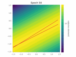
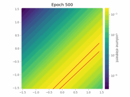
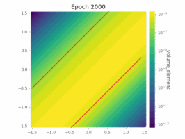
Figure G.1: Evolution of the volume element over training in a network trained to perform an XOR classification task (single hidden layer, two hidden units). Red lines indicate the decision boundaries of the network. See Appendix G.1 for experimental details and visualizations for higher hidden dimensions. Note that for two hidden unit case, the curvature is identically zero.

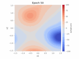
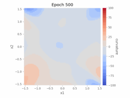
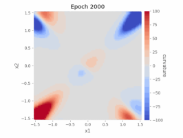
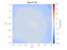
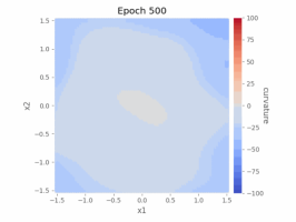
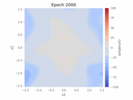
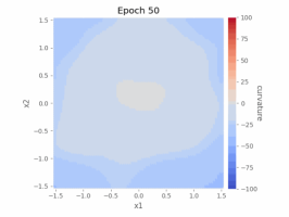
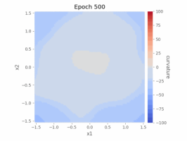
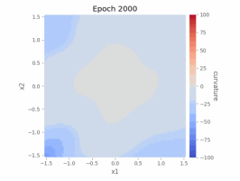
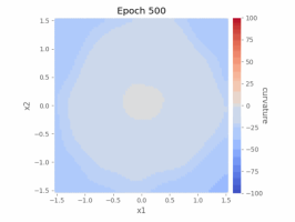
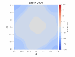
Figure G.2: Ricci curvature for XOR classification, with an architecture [2, $w$, 2] for $w=10$ (first row), $w=100$ (second row), $w=250$ (third row), and $w=500$ (forth row) hidden units across different epochs. As the number of hidden units increase, the curvature structure grows increasingly regularized and spherically symmetric.

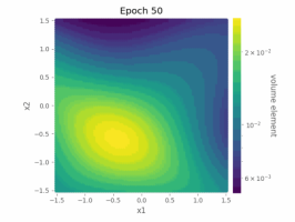
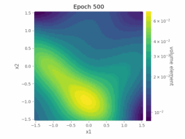
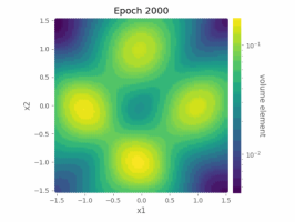
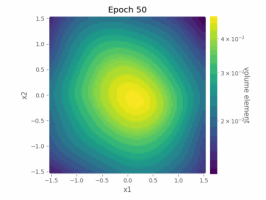
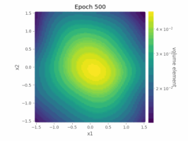
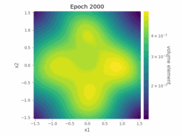
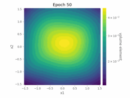
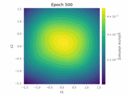
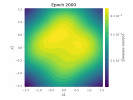
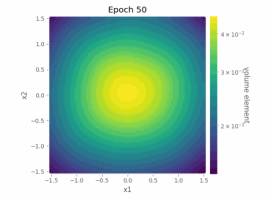
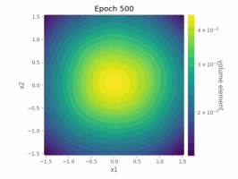
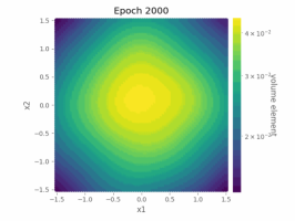
Figure G.3: Volume element for XOR classification, with an architecture [2, $w$, 2] for $w=10$ (first row), $w=100$ (second row), $w=250$ (third row), and $w=500$ (forth row) hidden units across different epochs. The volume element structures likewise become spherically symmetric as the number of hidden units increase.

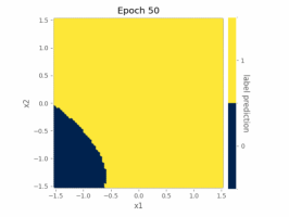
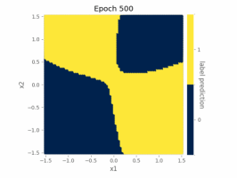
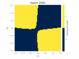
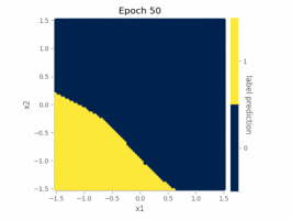
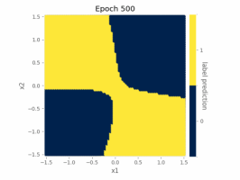
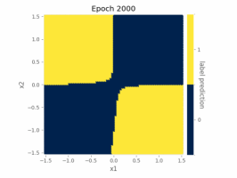
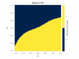
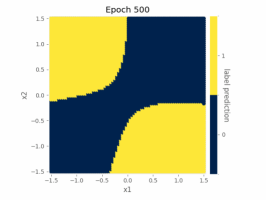
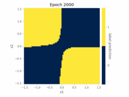
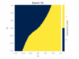
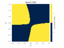
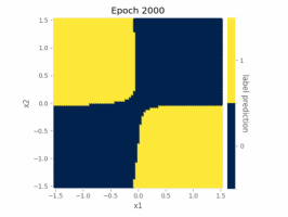
Figure G.4: Prediction for XOR classification, with architecture [2, $w$, 2] for $w=10$ (first row), $w=100$ (second row), $w=250$ (third row), and $w=500$ (forth row) hidden units across different epochs. As the hidden units increase, the prediction boundary converges to XOR quicker.

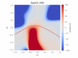
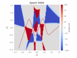
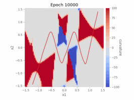
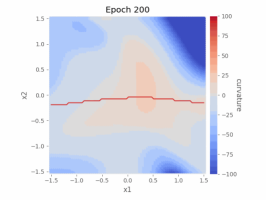
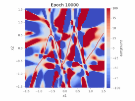
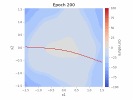
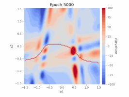
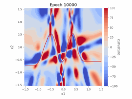
Figure G.5: Evolution of the Ricci curvature over training in a network trained to classify points separated by a sinusoidal boundary (single hidden layer with 5 hidden units (top), 20 hidden units (mid), and 250 hidden units (bottom)), clipped between -100 and 100 for visualization purposes. Red lines indicate the decision boundaries of the network. More hidden units offer smoother curvature transition when traversing the boundary, though the pattern presented here is less illustrative than the volume element in Figure 2.

G.2 Shallow networks trained to classify MNIST digits

We next compute the metric induced on input space by shallow networks trained to classify MNIST digits (LeCun et al., 2010). Single-hidden-layer fully-connected networks are initialized with widths $[784,2000,10]$, representing a modest 2.6-fold representational expansion, and trained on the 60000 $28\times 28$ pixel handwritten digit images for MNIST dataset and 120000 MNIST plus ambiguous MNIST digit images of the same size for Dirty MNIST dataset. We perform a 75/25 train test split, and no preprocessing is made on either training or testing set. Batches of 1000 images and their labels from the training set (numbers $0-9$) are fed to the network for 200 epochs; the networks are trained via the Adam optimizer (learning rate 0.001, weight decay $10^{-4}$) with negative log-likelihood loss. At the end of 200 epochs both training and testing accuracy exceed 95%. The metric induced by the trained network at a series of input images is then computed with autograd, e.g., PyTorch (Paszke et al., 2019). Here, as in Appendix G.1, we use float64 precision (Kochurov et al., 2020; Miolane et al., 2020; Mishne et al., 2022).

We give two styles of visualization: linear interpolation and plane spanning. For linear interpolation, the images we consider are images $\mathbf{y}_{i}$ interpolated between two test images $\mathbf{x}_{1},\mathbf{x}_{2}$ as follows: $\mathbf{y}(t)=(1-t)\mathbf{x}_{1}+t\mathbf{x}_{2}$ for $t\in[0,1]$; for plane spanning, the images are all in the plane spanned by three random test samples assigned at the edge of a unit equilateral triangle, so that each edge of the triangle correspond to the linear interpolation as previously noted. Concretely, we consider $\mathbf{y}(t_{1},t_{2},t_{3})=t_{1}\mathbf{x}_{1}+t_{2}\mathbf{x}_{2}+t_{3}\mathbf{x}_{3}$ for $\{t_{1},t_{2},t_{3}\in[0,1]:t_{1}+t_{2}+t_{3}=1\}$. Eigenvalues of the metric matrix $g_{\mu\nu}$ tend to become small as training progresses, and so, due to the high dimensionality of the input space, the metric $\sqrt{\det g_{\mu\nu}}$ becomes minuscule and difficult to compute within machine precision. Therefore, instead of $\sqrt{\det g_{\mu\nu}}$, we compute its logarithm (for efficiency, in production, we compute the log of the singular values of the Jacobians $\partial_{\mu}\Phi_{i}$ so as to avoid the complexity of large matrix multiplication in figuring out the metric). We find that this log volume element consistently grows (relatively) large at input images near the decision boundary, as shown in Figure 3 for the linear interpolation and the plane spanning.

As a preliminary investigation of geometry beyond interpolated low-dimensional slices in pixel space, we consider the Dirty-MNIST dataset (Mukhoti et al., 2021), which consists of VAE-generated ambiguous digit images. We also report the distribution of volume element at train and test samples in Figure G.13 for MNIST and Dirty MNIST digits 0, 7, and 9. In the large, the volume element evaluated at the ambiguous images is larger than at the clean images, which is consistent with Hypothesis 1. A more rigorous investigation, however, is required to support such a claim.

We conclude this experiment by commenting on the numerical stability of the computations described above. In addition to the geometric quantities, we also examine the numerical singularity of the metrics. Figure G.11 visualizes the full eigenvalue spectrum of at the anchor points corresponding to Figure G.9. As training progresses, the decay becomes slower initially, but expedites at respective tails, potentially as a manipulation by the network to contract local volumes compared to the boundary towards a better generalization, whose exact mechanism should be subject to further scrutiny. Importantly, note that all eigenvalues are of reasonable log scale in the float64 paradigm within 200 training epochs. Unfortunately, this may not hold when we increase the training epochs or perturb other hyperparameters. The tail eigenvalues would become too small even in the float64 range (smaller than $10^{-320}$, perilously close to the smallest positive number a float64 object can hold), and subsequent arithmetic operations break down. This close-to-singular behavior of the metric is ticklish and inevitable, and the naive solution of imposing threshold below which eigenvalues are discarded for volume element computation may risk not observing the central message of this paper that the volume element is large at the boundary since only parts of the eigenspectrum is taken into consideration.

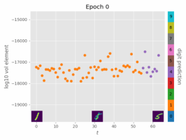
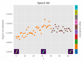
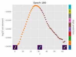
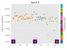
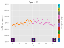
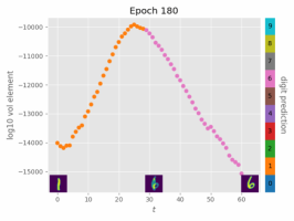
Figure G.6: $\log(\sqrt{\det g})$ induced at interpolated images between 1 and 5 (top row) and 1 and 6 (bottom row) by networks trained to classify MNIST digits. Sample images are visualized at the endpoints and midpoint for each set. Each line is colored by its prediction at the interpolated region and end points. As training progresses, the volume elements bulge in the middle (near decision boundary) and taper off at both endpoints. See Appendix G.2 for experimental details.

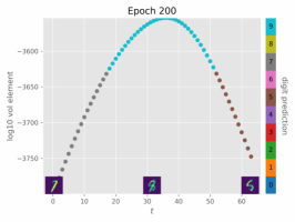
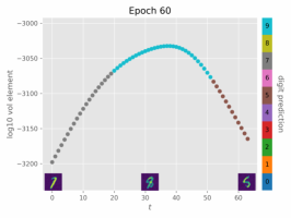
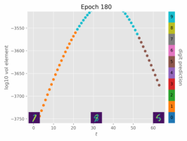
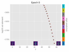
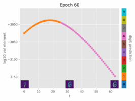
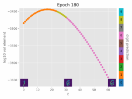
Figure G.7: $\log(\sqrt{\det g})$ induced at interpolated images between 1 and 5 (top row) and 1 and 6 (bottom row) by networks trained to classify Dirty MNIST digits. Sample images are visualized at the endpoints and midpoint for each set. Each line is colored by its prediction at the interpolated region and end points. As training progresses, the volume elements bulge in the middle (near decision boundary) and taper off at both endpoints. See Appendix G.2 for experimental details.

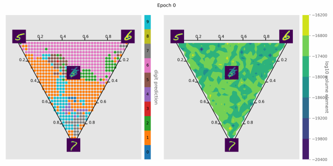
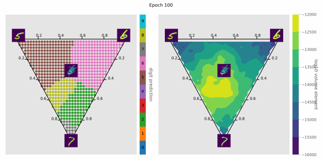
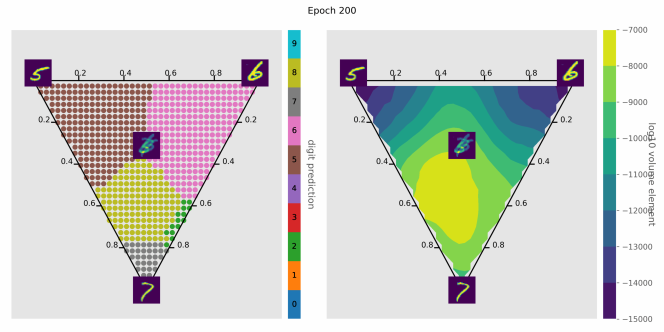
Figure G.8: Digit predictions and $\log(\sqrt{\det g})$ for the hyperplane spanned by three randomly sampled training point (5, 6, and 7) across different epochs.

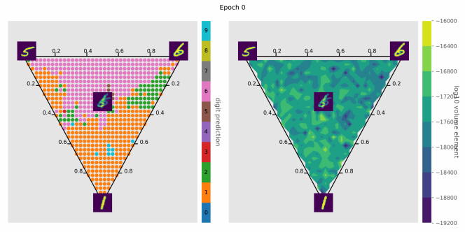
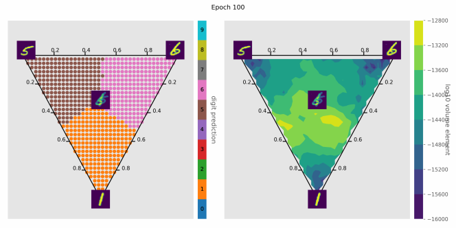
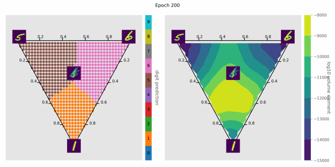
Figure G.9: Digit predictions and $\log(\sqrt{\det g})$ for the hyperplane spanned by three randomly sampled training point (5, 6, and 1) across different epochs.

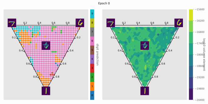
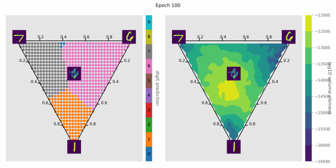
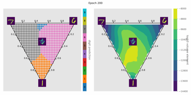
Figure G.10: Digit predictions and $\log(\sqrt{\det g})$ for the hyperplane spanned by three randomly sampled training point (7, 6, and 1) across different epochs.

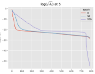
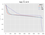
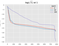
Figure G.11: The base-10 logarithms of the square roots of non-zero eigenvalues $\lambda_{i}$ of the metric $g$ at anchor points 5, 6, and 1 corresponding to Figure G.9

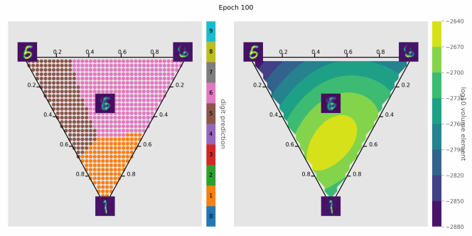
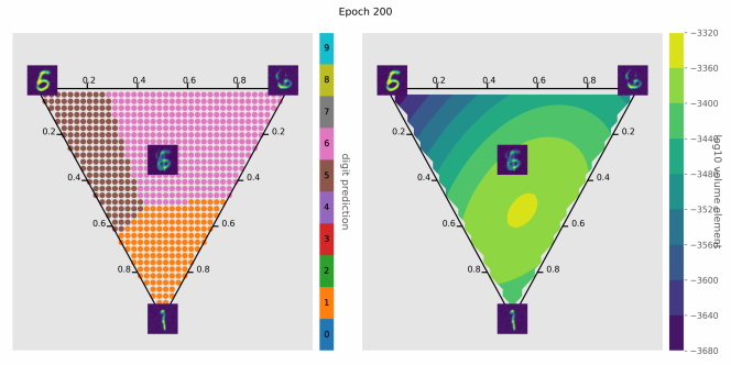
Figure G.12: Digit predictions and $\log(\sqrt{\det g})$ for the hyperplane spanned by three randomly sampled training point (5, 6, and 1 in Dirty MNIST) across different epochs.

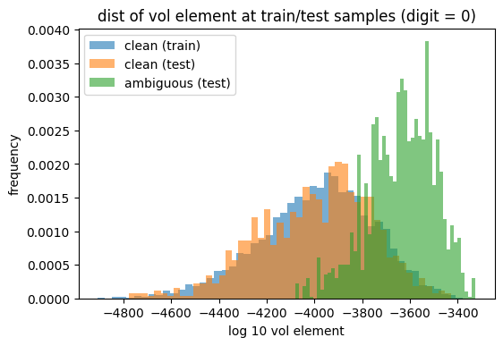
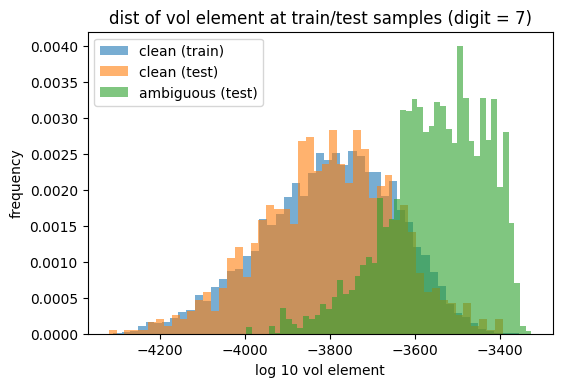
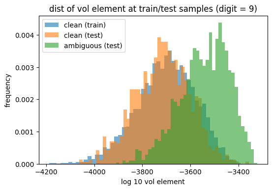
Figure G.13: Vol element distribution of three different samples: clean MNIST (train), clean MNIST (test), and ambiguous MNIST (test) samples of class 0, 7, and 9 respectively, using model trained only on the training set of clean MNIST for 200 epochs. Assuming equal variance, all groups yield a $p<10^{-4}$ for two-sample $t$-test between clean and ambiguous samples.

G.3 ResNets trained on CIFAR-10

Finally, we experiment on a deep network trained to classify CIFAR-10 images. CIFAR-10 contains 60000 train and 10000 test images, each of a size $3\times 32\times 32$ (Krizhevsky, 2009). 10 classes of images cover plane, car, bird, cat, deer, dog, frog, horse, ship, and truck, with an equal distribution in each class. Some preprocessing is made to boost performance: for training set, we pad each image for 4 pixels and crop at random places to keep it of size $32\times 32$, randomly horizontally flip images with probability 0.5, and translate each channel by subtracting (0.4914, 0.4822, 0.4465) and scale by dividing (0.2023, 0.1994, 0.2010); for testing, we only perform the translation and scaling (Liu et al., 2021). We use ResNet-34 (He et al., 2016) with GELU activation functions (Hendrycks and Gimpel, 2016), trained with SGD using a learning rate 0.01, weight decay $10^{-4}$, and momentum 0.9. Batches of 1024 images are fed to train for 200 epochs. Our ResNet code was adapted from the publicly-available implementation by Liu et al. (2021), distributed under an MIT License. At the final epoch the training accuracy reaches above 99% and testing accuracy around 92%.

The images we consider are generated from samples in the preprocessed testing set and interpolated in the same fashion as in the MNIST dataset (Appendix G.2). The geometric quantity considered here is likewise $\log({\sqrt{\det g}})$ and is computed using autograd. For demonstration purposes, although geometric quantities are computed on preprocessed images, the images in Figures throughout this paper are their unpreprocessed counterparts. In general, the message in CIFAR-10 experiment is consistent with our findings that along decision boundaries we observe large volume elements but is less clear: The linear interpolation plot in Figure G.14 demonstrate similar behaviors as in its counterpart in Figure G.6; Figure G.16, Figure G.17, and Figure G.18 each visualizes the convex hull anchored by different combinations of classes and demonstrates much more convoluted decision boundaries in the interpolated space. Likewise, the volume element enlarges when traversing the decision boundaries and stays small within a class prediction region.

We also visualized the volume element expansion factor induced by metrics pulled back from respective blocks of ResNet-34. The readouts from layer 1 to 4 are patched with a average pooling with kernel sizes $(16,8),(8,8),(8,4),(4,4)$ to ensure a output dimension of 512 from each intermediate layer and abide by the memory constraints of the computations. Figure 6 and Figure 7 both demonstrated consistent result with the final layer pullback metrics. Interestingly, later blocks show more contrasts than early ones, potentially suggesting that the distinguishing features of images are mostly capture by the last block.

In addition to the convex hull visualization, we provide the affine hull (i.e. the region extrapolated from the anchor points) in Figure G.19 along with the entropy of the softmax outputs by ResNet-34. The entropy here is computed with $\log_{10}$ to scale values between 0 and 1 for this 10 class classification task. Note that places with high entropy (more uncertainty) not only delineate the decision boundaries but also correspond to places with large volume element.

Moreover, we also show that volume element does not expand in regions away from the decision boundaries. We illustrate this phenomenon in Figure G.20 by sampling images from the same class to span the plane and conclude that the volume element expansion is only pronounced when there is an explicit decision boundary, regardless of it being a correct one.

The same pattern is observed for the same achitecture but with ReLU activation. Even though ReLU is not differentiable, it still yields consistent prediction as in the GELU cases where the volume element expands near the decision boundaries. These are demonstrated by the linear interpolation in Figure G.21 and convex hull plane visualization in Figure G.23, G.24, G.25 and affine hull plane visualization in Figure G.26. Examination of the eigen spectrum in Figure G.22 does not flag any numerical issues in computations

We conclude this section by commenting on the memory consumption. Note that for this experiment only, we enforce float32 out of memory concerns. This fortunately does not pose a numerical challenge since all eigenvalues are in a reasonable range (shown in Figure G.15), bounded away from the smallest positive number float32 can hold ($10^{-38}$). However, the memory issue effectively constraints the choice of our model, since the exact log volume element at a single training sample computed through autograd for deeper network (e.g. ResNet-50, ResNet-101) requires more than 80GB, exceeding the largest memory configuration of any single publicly available GPU as of the time of writing (NVIDIA A100). To enable the study of larger models, it would be useful to have an approximation for the volume element with tractable memory footprint in the future.

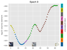
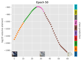
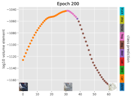
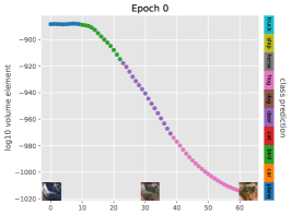
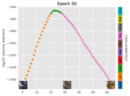
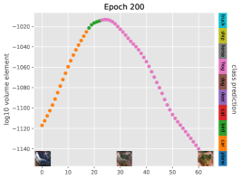
Figure G.14: $\log(\sqrt{\det g})$ induced at interpolated images between a car and a dog (top row) and between a car and a frog (bottom row) by ResNet-34 trained to classify CIFAR-10 digits. Sample images are visualized at the endpoints and midpoint for each set. Each line is colored by its prediction at the interpolated region and end points. As training progresses, the volume elements bulge in the middle (near decision boundary) and taper off at both endpoints. See Appendix G.3 for experimental details.

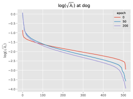
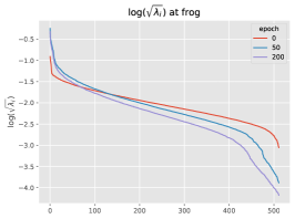
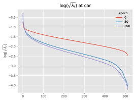
Figure G.15: The base-10 logarithms of square roots of the eigenvalues $\lambda_{i}$ of the metric $g$ at the anchor points in Figure G.16: dog (left), frog (mid), and car (right). As training proceeds, the spectrum is shifted downward and consequently the volume element decreases at these points.

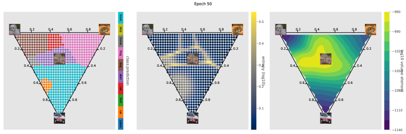
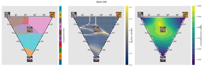
Figure G.16: Digit predictions, $\log_{10}(\text{entropy})$, and $\log_{10}(\sqrt{\det g})$ for the hyperplane spanned by three randomly sampled training point a dog, a frog, and a car across different epochs.

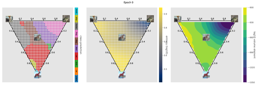
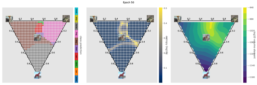
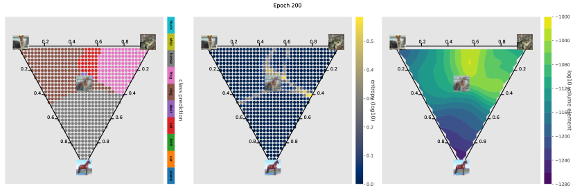
Figure G.17: Digit predictions, $\log_{10}(\text{entropy})$, and $\log_{10}(\sqrt{\det g})$ for the hyperplane spanned by three randomly sampled training point a dog, a frog, and a horse across different epochs.

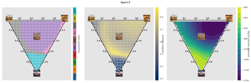
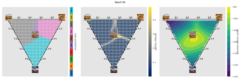
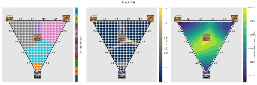
Figure G.18: Digit predictions, $\log_{10}(\text{entropy})$, and $\log_{10}(\sqrt{\det g})$ for the hyperplane spanned by three randomly sampled training point a horse, a frog, and a car across different epochs.

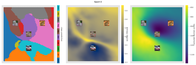
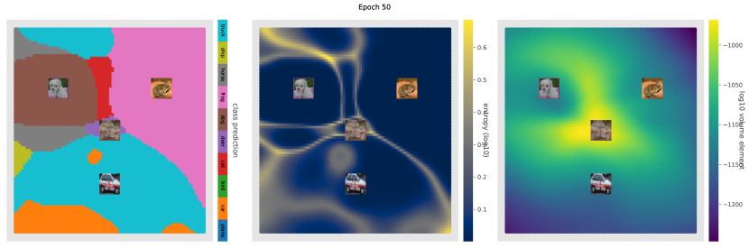
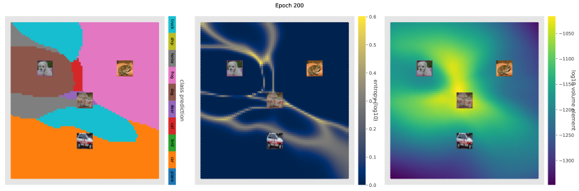
Figure G.19: Digit predictions and $\log(\sqrt{\det g})$ for the hyperplane spanned by three randomly sampled training point a dog, a frog, and a car across different epochs. The entire affine hull (instead of the convex hull) is visualized. The middle panel is the entropy of the softmax-ed probabilities of the ResNet-34 outputs. Places with high entropy demarcate the decision boundary as well as regions with relatively large volume element as expected, though less clear in the latter case.

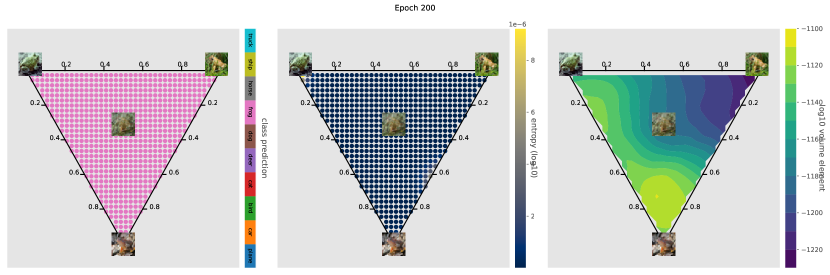
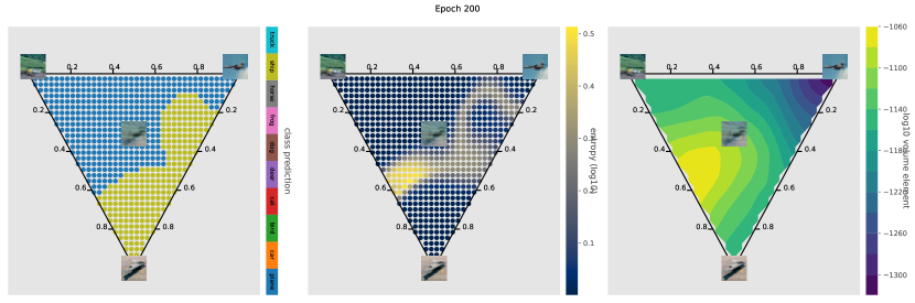
Figure G.20: Regions away from decision boundaries do not have a clear volume element pattern: we randomly select three figures from the same class (top: frogs, bottom: planes) and perform the plane extrapolation. We visualize digit predictions, $\log_{10}(\text{entropy})$, and $\log_{10}(\sqrt{\det g})$ at the end of training for both cases. The top graph predicts frog universally with slight volume element variation across the landscape; the bottom graph has an incorrect prediction of plane (treating it as a ship), and creates an artifact of a decision boundary, which explains the vol element expansion at near that region.

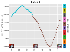
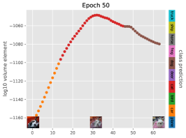
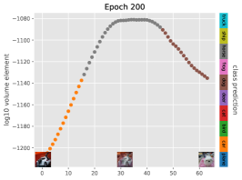
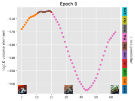
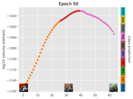
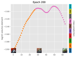
Figure G.21: $\log(\sqrt{\det g})$ induced at interpolated images between a car and a dog (top row) and between a car and a frog (bottom row) by ResNet-34 with ReLU activation trained to classify CIFAR-10 digits. Sample images are visualized at the endpoints and midpoint for each set. Each line is colored by its prediction at the interpolated region and end points. As training progresses, the volume elements bulge in the middle (near decision boundary) and taper off at both endpoints. See Appendix G.3 for experimental details.

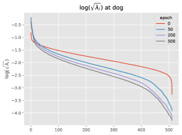
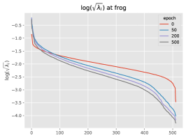
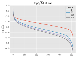
Figure G.22: The base-10 logarithms of square roots of the eigenvalues $\lambda_{i}$ of the metric $g$ at the anchor points in Figure G.23: dog (left), frog (mid), and car (right). As training proceeds, the spectrum is shifted downward and consequently the volume element decreases at these points.

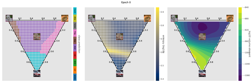
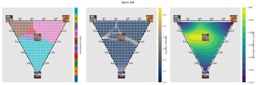
Figure G.23: Same as Figure G.16 but with ReLU activation. Digit predictions, $\log_{10}(\text{entropy})$, and $\log_{10}(\sqrt{\det g})$ for the hyperplane spanned by three randomly sampled training point a dog, a frog, and a car across different epochs.

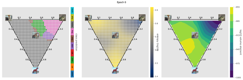
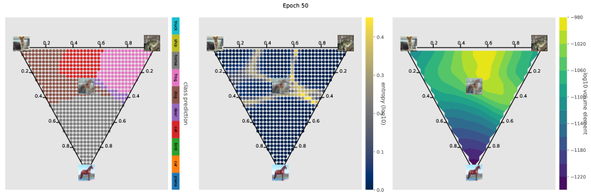
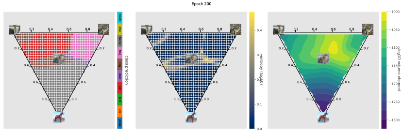
Figure G.24: Same as Figure G.17 but iwth ReLU activation. Digit predictions, $\log_{10}(\text{entropy})$, and $\log_{10}(\sqrt{\det g})$ for the hyperplane spanned by three randomly sampled training point a dog, a frog, and a horse across different epochs.

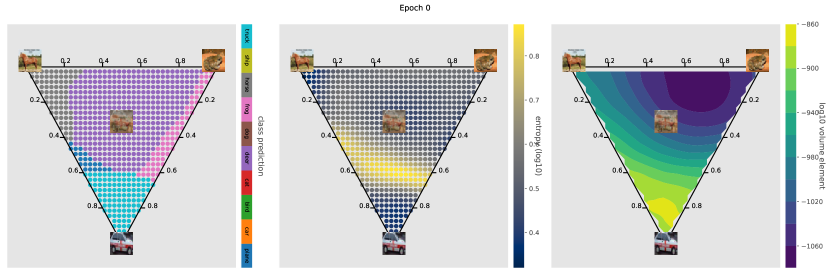
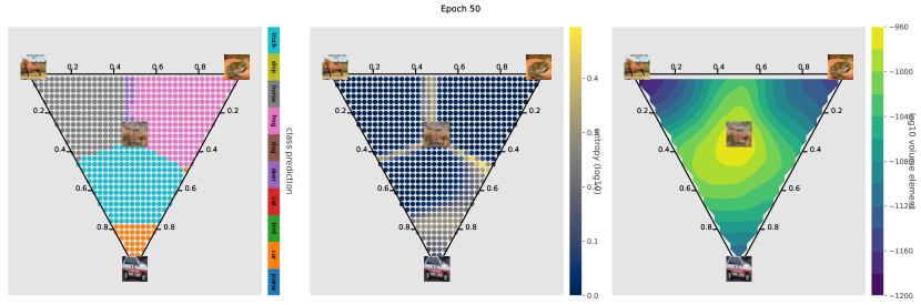
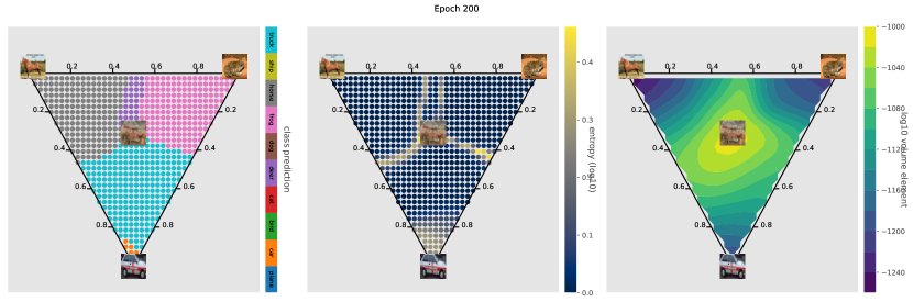
Figure G.25: Same as Figure G.18 but with ReLU activation. Digit predictions, $\log_{10}(\text{entropy})$, and $\log_{10}(\sqrt{\det g})$ for the hyperplane spanned by three randomly sampled training point a horse, a frog, and a car across different epochs.

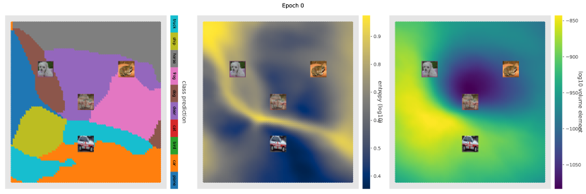
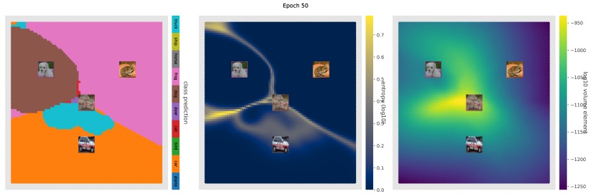
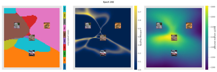
Figure G.26: Same as Figure G.19 but with ReLU activation. Predictions and $\log(\sqrt{\det g})$ for the hyperplane spanned by three randomly sampled training point a dog, a frog, and a car across different epochs. The entire affine hull (instead of the convex hull) is visualized. The middle panel is the entropy of the softmax-ed probabilities of the ResNet-34 outputs. Places with high entropy demarcate the decision boundary as well as regions with relatively large volume element as expected, though less clear in the latter case.

G.4 Self-supervised learning on CIFAR-10: Barlow Twins and SimCLR

Our hypothesis likewise extends to self-supervised learning frameworks. We employ the Barlow Twins architecture (Zbontar et al., 2021) with a ResNet-34 backbone, GELU activation, and a single-layer projector of dimension 256. We train the network for 1000 epochs with SGD optimizer, a learning rate of 0.01, weight decay $10^{-4}$, and a batch size of 1024. In the following we report the model performance at initialization, 200 epochs, and 1000 epochs respectively.

Data augmentation is done slightly differently from training end-to-end ResNet-34 as above and we follow exactly the same procedure as in (Zbontar et al., 2021): random crop to 32 by 32 images, random horizontal flip with probability 0.5, a color jitter with brightness=0.4, contrast=0.4, saturation=0.2, hue=0.1, and probability 0.8, random grayscale with probability 0.2, a gaussian blur with probability 1.0 and 0.1 for two augmented inputs, solarization with probability 0 and 0.2 for two augmented inputs, and finally a normalization by subtracting [0.485, 0.456, 0.406] and dividing by [0.229, 0.224, 0.225] channelwise.

Unlike supervised training, in the self-supervised framework the network is not exposed to labels during training. The predictor is separately trained using a multiclass logistic regression with an $l_{2}$ regularization of 1 on features obtained by the ResNet-34 backbone at different snapshots of the training epochs. For ResNet-34 in particular each image is represented by a vector of dimension 512. At the end of 1000 epochs, a multiclass logistic regression is able to reach 84% accuracy on training set and 70% accuracy on testing set. We acknowledge that the performance can be further improved if we use a deeper backbone (e.g. ResNet 50) or a more expressive projector appended to the ResNet backbone. Figure G.27 shows the linear interpolation between two samples and Figure G.30, G.29, G.28 show the convex hull generated by three samples. Likewise, we also display the eigenspectrum in Figure G.31, which does not indicate any numerical issues.

One intriguing phenomenon is that we observe the opposite behavior for the contrastive learning model SimCLR (Chen et al., 2020). The volume element is now dipping at decision boundaries. We suspect that this is due to SimCLR’s explicit requirement that the embeddings lie on a unit sphere. As a result, it is possible that pulling back the Euclidean metric from embedding space is no longer appropriate, and one should instead pull back the flat metric on the sphere. Investigating this phenomenon could be an interesting topic for future work. One demonstration of this phenomenon is displayed in figure G.33, G.35, G.34.

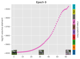
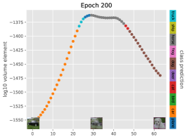
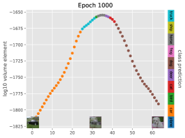
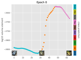
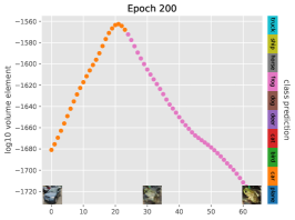
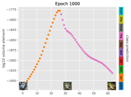
Figure G.27: $\log(\sqrt{\det g})$ induced at interpolated images between a car and a dog (top row) and between a car and a frog (bottom row) by Barlow Twins with ResNet-34 backbone and a GELU activation. Sample images are visualized at the endpoints and midpoint for each set. Each line is colored by its prediction at the interpolated region and end points. As training progresses, the volume elements bulge in the middle (near decision boundary) and taper off at both endpoints. See Appendix G.4 for experimental details.

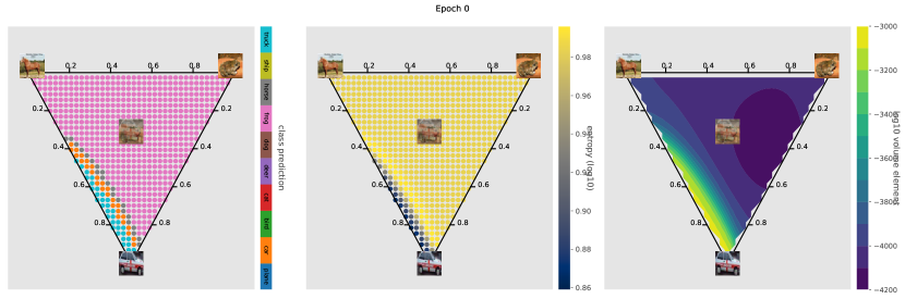
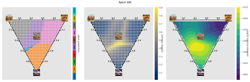
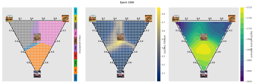
Figure G.28: Digit predictions, $\log_{10}(\text{entropy})$, and $\log_{10}(\sqrt{\det g})$ for the hyperplane spanned by three randomly sampled training point a horse, a frog, and a car across different epochs for Barlow Twins with ResNet-34 backbone using GELU activation.

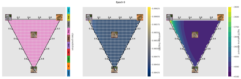
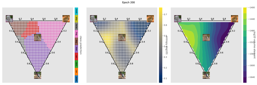
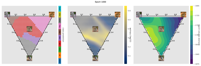
Figure G.29: Digit predictions, $\log_{10}(\text{entropy})$, and $\log_{10}(\sqrt{\det g})$ for the hyperplane spanned by three randomly sampled training point a dog, a frog, and a horse across different epochs for Barlow Twins with ResNet-34 backbone using GELU activation.

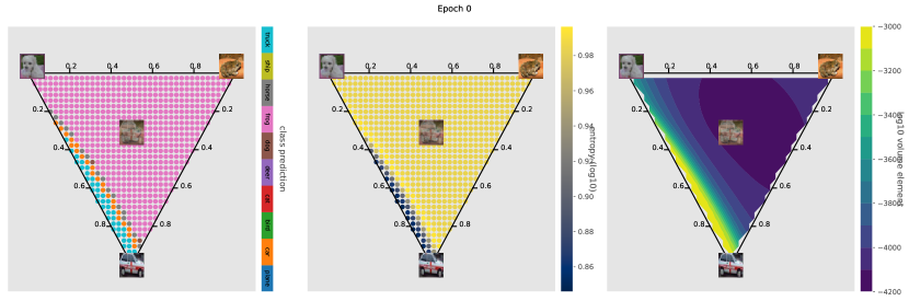
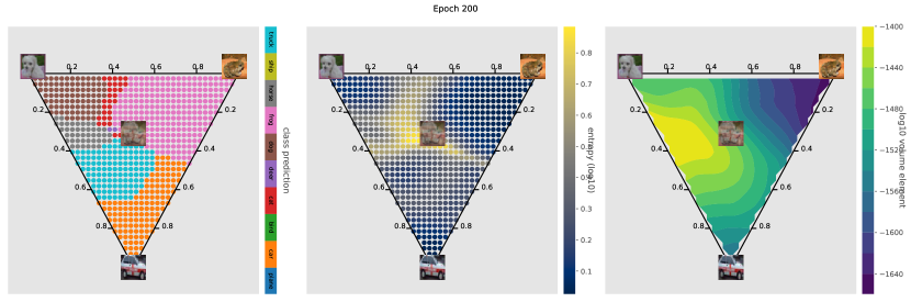
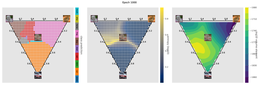
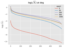
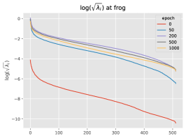
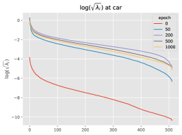
Figure G.30: Digit predictions, $\log_{10}(\text{entropy})$, and $\log_{10}(\sqrt{\det g})$ for the hyperplane spanned by three randomly sampled training point a dog, a frog, and a car across different epochs for Barlow Twins with ResNet-34 backbone using GELU activation.

Figure G.31: The base-10 logarithms of square roots of the eigenvalues $\lambda_{i}$ of the metric $g$ at the anchor points in Figure G.30: dog (left), frog (mid), and car (right) for Barlow Twins with ResNet-34 backbone using GELU activation. As training proceeds, the spectrum is initially shifted upward and then shifted downward and consequently the volume element decreases at these points.

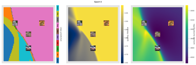
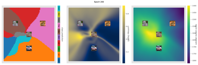
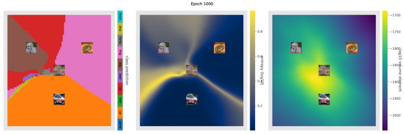
Figure G.32: Digit predictions, $\log_{10}(\text{entropy})$, and $\log_{10}(\sqrt{\det g})$ for the affine hull spanned by three randomly sampled training point a dog, a frog, and a car across different epochs for Barlow Twins with ResNet-34 backbone using GELU activation. This corresponds to Figure G.30.

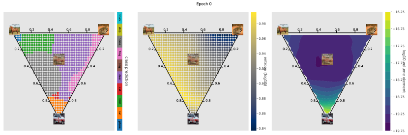
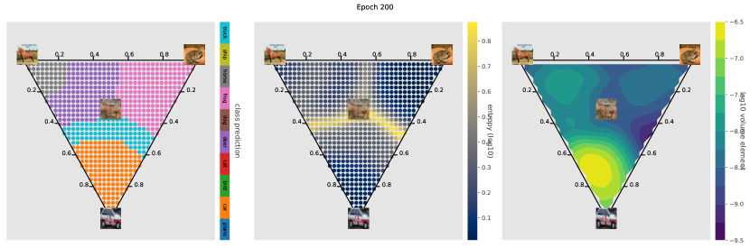
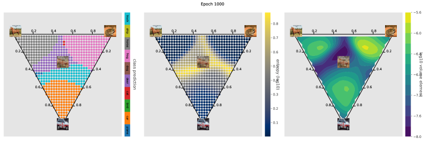
Figure G.33: Digit predictions, $\log_{10}(\text{entropy})$, and $\log_{10}(\sqrt{\det g})$ for the hyperplane spanned by three randomly sampled training point a horse, a frog, and a car across different epochs for SimCLR with ResNet-34 backbone using GELU activation. This contradicts our predictions since the volume elements dip at decision boundaries, possibly due to the inappropriateness of approximating a sphere using a linear interpolation.

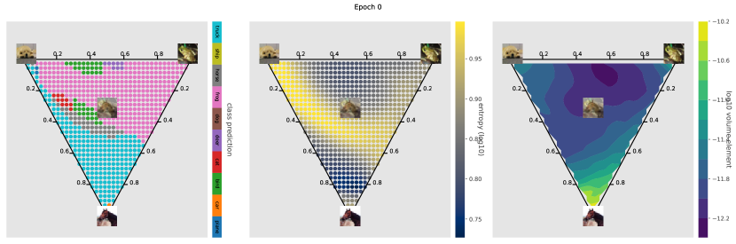
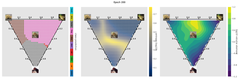
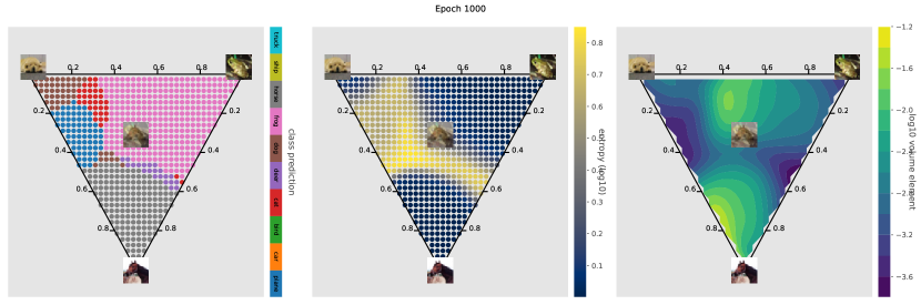
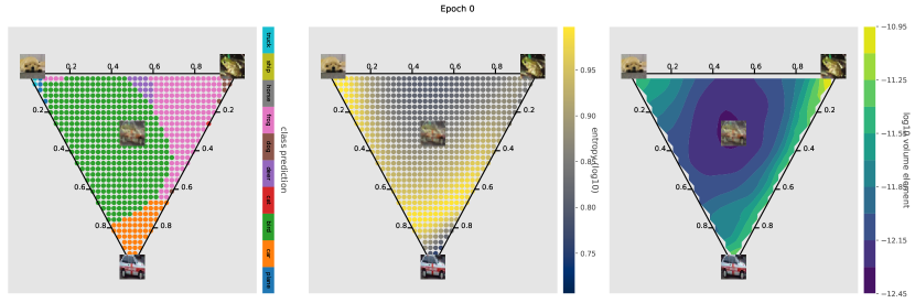
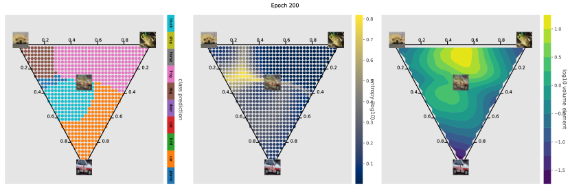
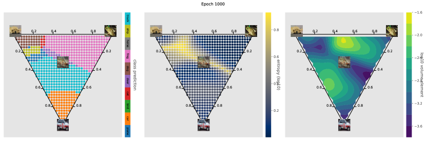
Figure G.34: Digit predictions, $\log_{10}(\text{entropy})$, and $\log_{10}(\sqrt{\det g})$ for the hyperplane spanned by three randomly sampled training point a dog, a frog, and a horse across different epochs for SimCLR with ResNet-34 backbone using GELU activation. This contradicts our predictions since the volume elements dip at decision boundaries, possibly due to the inappropriateness of approximating a sphere using a linear interpolation.

Figure G.35: Digit predictions, $\log_{10}(\text{entropy})$, and $\log_{10}(\sqrt{\det g})$ for the hyperplane spanned by three randomly sampled training point a dog, a frog, and a car across different epochs for SimCLR with ResNet-34 backbone using GELU activation. This contradicts our predictions since the volume elements dip at decision boundaries, possibly due to the inappropriateness of approximating a sphere using a linear interpolation.

G.5 Data and code availability

All datasets used in this work are either programmatically generated (Appendix G.1) or publicly available (Appendices G.2, G.3, and G.4; LeCun et al. (2010) and Krizhevsky (2009)). PyTorch Paszke et al. (2019) code to train all models and generate figures is available on GitHub at https://github.com/Pehlevan-Group/nn_curvature. As noted above, our ResNet implementation is adapted from Liu et al. (2021)’s MIT-licensed implementation.

All models were trained on the Harvard Cannon HPC cluster equipped with NVIDIA SMX4-A100-80GB GPUs (https://www.rc.fas.harvard.edu/).

References

• Abbas et al. (2023) Amro Abbas, Kushal Tirumala, Dániel Simig, Surya Ganguli, and Ari S. Morcos. Semdedup: Data-efficient learning at web-scale through semantic deduplication. arXiv, 2023. doi:10.48550/arXiv.2303.09540.
• Acosta et al. (2022) Francisco E. Acosta, Sophia Sanborn, Khanh Dao Duc, Manu Madhav, and Nina Miolane. Quantifying local extrinsic curvature in neural manifolds. arXiv, 2022. doi:10.48550/ARXIV.2212.10414. URL https://arxiv.org/abs/2212.10414.
• Amari and Wu (1999) Shun-ichi Amari and Si Wu. Improving support vector machine classifiers by modifying kernel functions. Neural Networks, 12(6):783–789, 1999. ISSN 0893-6080. doi:https://doi.org/10.1016/S0893-6080(99)00032-5. URL https://www.sciencedirect.com/science/article/pii/S0893608099000325.
• Amari et al. (2019) Shun-ichi Amari, Ryo Karakida, and Masafumi Oizumi. Statistical neurodynamics of deep networks: Geometry of signal spaces. Nonlinear Theory and Its Applications, IEICE, 10(4):322–336, 2019. URL https://www.jstage.jst.go.jp/article/nolta/10/4/10_322/_pdf/-char/en.
• Benfenati and Marta (2023a) Alessandro Benfenati and Alessio Marta. A singular Riemannian geometry approach to deep neural networks: II. Reconstruction of 1-D equivalence classes. Neural Networks, 158:344–358, 2023a. ISSN 0893-6080. doi:https://doi.org/10.1016/j.neunet.2022.11.026. URL https://www.sciencedirect.com/science/article/pii/S0893608022004671.
• Benfenati and Marta (2023b) Alessandro Benfenati and Alessio Marta. A singular Riemannian geometry approach to deep neural networks: I. Theoretical foundations. Neural Networks, 158:331–343, 2023b. ISSN 0893-6080. doi:https://doi.org/10.1016/j.neunet.2022.11.022. URL https://www.sciencedirect.com/science/article/pii/S0893608022004634.
• Bordelon and Pehlevan (2022) Blake Bordelon and Cengiz Pehlevan. Self-consistent dynamical field theory of kernel evolution in wide neural networks. In Alice H. Oh, Alekh Agarwal, Danielle Belgrave, and Kyunghyun Cho, editors, Advances in Neural Information Processing Systems, volume 35, 2022. URL https://openreview.net/forum?id=sipwrPCrIS.
• Bronstein et al. (2021) Michael M Bronstein, Joan Bruna, Taco Cohen, and Petar Veličković. Geometric deep learning: Grids, groups, graphs, geodesics, and gauges. arXiv preprint arXiv:2104.13478, 2021. URL https://geometricdeeplearning.com/.
• Burges (1999) Christopher J. C. Burges. Geometry and invariance in kernel based methods. In Bernhard Schölkopf, Christopher J. C. Burges, and Alexander J. Smola, editors, Advances in Kernel Methods: Support Vector Learning, page 89–116, Cambridge, MA, USA, 1999. MIT Press. ISBN 0262194163.
• Chami et al. (2020) Ines Chami, Adva Wolf, Da-Cheng Juan, Frederic Sala, Sujith Ravi, and Christopher Ré. Low-dimensional hyperbolic knowledge graph embeddings. arXiv preprint arXiv:2005.00545, 2020.
• Chen et al. (2020) Ting Chen, Simon Kornblith, Mohammad Norouzi, and Geoffrey Hinton. A simple framework for contrastive learning of visual representations. In Hal Daumé III and Aarti Singh, editors, Proceedings of the 37th International Conference on Machine Learning, volume 119 of Proceedings of Machine Learning Research, pages 1597–1607. PMLR, 13–18 Jul 2020. URL https://proceedings.mlr.press/v119/chen20j.html.
• Cho and Saul (2009) Youngmin Cho and Lawrence K Saul. Kernel methods for deep learning. In Y. Bengio, D. Schuurmans, J. Lafferty, C. Williams, and A. Culotta, editors, Advances in Neural Information Processing Systems, volume 22. Curran Associates, Inc., 2009. URL https://proceedings.neurips.cc/paper/2009/file/5751ec3e9a4feab575962e78e006250d-Paper.pdf.
• Cho and Saul (2011) Youngmin Cho and Lawrence K Saul. Analysis and extension of arc-cosine kernels for large margin classification. arXiv preprint arXiv:1112.3712, 2011. doi:10.48550/ARXIV.1112.3712. URL https://arxiv.org/abs/1112.3712.
• Chung et al. (2018) SueYeon Chung, Daniel D. Lee, and Haim Sompolinsky. Classification and geometry of general perceptual manifolds. Phys. Rev. X, 8:031003, Jul 2018. doi:10.1103/PhysRevX.8.031003. URL https://link.aps.org/doi/10.1103/PhysRevX.8.031003.
• Cohen et al. (2018) Taco S Cohen, Mario Geiger, Jonas Köhler, and Max Welling. Spherical CNNs. arXiv preprint arXiv:1801.10130, 2018.
• Cohen et al. (2020) Uri Cohen, SueYeon Chung, Daniel D. Lee, and Haim Sompolinsky. Separability and geometry of object manifolds in deep neural networks. Nature Communications, 11(1):746, Feb 2020. ISSN 2041-1723. doi:10.1038/s41467-020-14578-5. URL https://doi.org/10.1038/s41467-020-14578-5.
• Daniely et al. (2016) Amit Daniely, Roy Frostig, and Yoram Singer. Toward deeper understanding of neural networks: The power of initialization and a dual view on expressivity. In D. Lee, M. Sugiyama, U. Luxburg, I. Guyon, and R. Garnett, editors, Advances in Neural Information Processing Systems, volume 29. Curran Associates, Inc., 2016. URL https://proceedings.neurips.cc/paper/2016/file/abea47ba24142ed16b7d8fbf2c740e0d-Paper.pdf.
• (18) DLMF. NIST Digital Library of Mathematical Functions. http://dlmf.nist.gov/, Release 1.1.1 of 2021-03-15, 2021. URL http://dlmf.nist.gov/. F. W. J. Olver, A. B. Olde Daalhuis, D. W. Lozier, B. I. Schneider, R. F. Boisvert, C. W. Clark, B. R. Miller, B. V. Saunders, H. S. Cohl, and M. A. McClain, eds.
• Dodson and Poston (1991) Christopher Terence John Dodson and Timothy Poston. Tensor Geometry: The Geometric Viewpoint and its Uses. Springer Berlin Heidelberg, Berlin, Heidelberg, 1991. ISBN 978-3-642-10514-2. doi:10.1007/978-3-642-10514-2_11. URL https://doi.org/10.1007/978-3-642-10514-2_11.
• Esteves et al. (2018) Carlos Esteves, Christine Allen-Blanchette, Ameesh Makadia, and Kostas Daniilidis. Learning SO(3) equivariant representations with spherical CNNs. In Proceedings of the European Conference on Computer Vision (ECCV), pages 52–68, 2018.
• Goodfellow et al. (2014) Ian J. Goodfellow, Jonathon Shlens, and Christian Szegedy. Explaining and harnessing adversarial examples. arXiv, 2014. doi:10.48550/ARXIV.1412.6572. URL https://arxiv.org/abs/1412.6572.
• Gu et al. (2018) Albert Gu, Frederic Sala, Beliz Gunel, and Christopher Ré. Learning mixed-curvature representations in product spaces. In International conference on learning representations, 2018.
• Gupta (1999) Anupam Gupta. Embedding tree metrics into low dimensional euclidean spaces. In Proceedings of the thirty-first annual ACM symposium on Theory of computing, pages 694–700, 1999.
• Hanin and Rolnick (2019a) Boris Hanin and David Rolnick. Complexity of linear regions in deep networks. In Kamalika Chaudhuri and Ruslan Salakhutdinov, editors, Proceedings of the 36th International Conference on Machine Learning, volume 97 of Proceedings of Machine Learning Research, pages 2596–2604. PMLR, 09–15 Jun 2019a. URL https://proceedings.mlr.press/v97/hanin19a.html.
• Hanin and Rolnick (2019b) Boris Hanin and David Rolnick. Deep ReLU networks have surprisingly few activation patterns. In H. Wallach, H. Larochelle, A. Beygelzimer, F. d'Alché-Buc, E. Fox, and R. Garnett, editors, Advances in Neural Information Processing Systems, volume 32. Curran Associates, Inc., 2019b. URL https://proceedings.neurips.cc/paper/2019/file/9766527f2b5d3e95d4a733fcfb77bd7e-Paper.pdf.
• Hauser and Ray (2017) Michael Hauser and Asok Ray. Principles of Riemannian geometry in neural networks. In I. Guyon, U. Von Luxburg, S. Bengio, H. Wallach, R. Fergus, S. Vishwanathan, and R. Garnett, editors, Advances in Neural Information Processing Systems, volume 30. Curran Associates, Inc., 2017. URL https://proceedings.neurips.cc/paper/2017/file/0ebcc77dc72360d0eb8e9504c78d38bd-Paper.pdf.
• He et al. (2016) Kaiming He, Xiangyu Zhang, Shaoqing Ren, and Jian Sun. Deep residual learning for image recognition. In 2016 IEEE Conference on Computer Vision and Pattern Recognition (CVPR), pages 770–778, 2016. doi:10.1109/CVPR.2016.90. URL https://ieeexplore.ieee.org/document/7780459.
• Hein and Andriushchenko (2017) Matthias Hein and Maksym Andriushchenko. Formal guarantees on the robustness of a classifier against adversarial manipulation. Advances in neural information processing systems, 30, 2017.
• Hendrycks and Gimpel (2016) Dan Hendrycks and Kevin Gimpel. Gaussian error linear units (GELUs). arXiv, 2016. doi:10.48550/ARXIV.1606.08415. URL https://arxiv.org/abs/1606.08415.
• Kaul and Lall (2020) Piyush Kaul and Brejesh Lall. Riemannian curvature of deep neural networks. IEEE Transactions on Neural Networks and Learning Systems, 31(4):1410–1416, 2020. doi:10.1109/TNNLS.2019.2919705.
• Khrulkov et al. (2020) Valentin Khrulkov, Leyla Mirvakhabova, Evgeniya Ustinova, Ivan Oseledets, and Victor Lempitsky. Hyperbolic image embeddings. In Proceedings of the IEEE/CVF Conference on Computer Vision and Pattern Recognition, pages 6418–6428, 2020.
• Klimovskaia et al. (2020) Anna Klimovskaia, David Lopez-Paz, Léon Bottou, and Maximilian Nickel. Poincaré maps for analyzing complex hierarchies in single-cell data. Nature communications, 11(1):2966, 2020.
• Kochurov et al. (2020) Max Kochurov, Rasul Karimov, and Serge Kozlukov. Geoopt: Riemannian optimization in PyTorch. arXiv preprint arXiv:2005.02819, 2020.
• Kornblith et al. (2019) Simon Kornblith, Mohammad Norouzi, Honglak Lee, and Geoffrey Hinton. Similarity of neural network representations revisited. In Kamalika Chaudhuri and Ruslan Salakhutdinov, editors, Proceedings of the 36th International Conference on Machine Learning, volume 97 of Proceedings of Machine Learning Research, pages 3519–3529. PMLR, 09–15 Jun 2019. URL https://proceedings.mlr.press/v97/kornblith19a.html.
• Krizhevsky (2009) Alex Krizhevsky. Learning multiple layers of features from tiny images. Technical report, University of Toronto, 2009. URL https://www.cs.toronto.edu/~kriz/cifar.html.
• Kuhnel et al. (2018) Line Kuhnel, Tom Fletcher, Sarang Joshi, and Stefan Sommer. Latent space non-linear statistics. arXiv, 2018. doi:10.48550/ARXIV.1805.07632. URL https://arxiv.org/abs/1805.07632.
• Kupeli (2013) Demir N Kupeli. Singular semi-Riemannian geometry, volume 366. Springer Science & Business Media, 2013. URL https://doi.org/10.1007/978-94-015-8761-7.
• LeCun et al. (2010) Yann LeCun, Corinna Cortes, and CJ Burges. MNIST handwritten digit database. ATT Labs [Online], 2, 2010. URL http://yann.lecun.com/exdb/mnist.
• LeCun et al. (2015) Yann LeCun, Yoshua Bengio, and Geoffrey Hinton. Deep learning. Nature, 521(7553):436–444, May 2015. ISSN 1476-4687. doi:10.1038/nature14539. URL https://doi.org/10.1038/nature14539.
• Lee et al. (2018) Jaehoon Lee, Jascha Sohl-Dickstein, Jeffrey Pennington, Roman Novak, Sam Schoenholz, and Yasaman Bahri. Deep neural networks as Gaussian processes. In International Conference on Learning Representations, 2018. URL https://openreview.net/forum?id=B1EA-M-0Z.
• Liu et al. (2021) Kuang Liu, Wei Yang, Peiwen Yang, and Felipe Ducau. Train CIFAR10 with PyTorch. Github, 02 2021. URL https://github.com/kuangliu/pytorch-cifar.
• Matthews et al. (2018) Alexander G. de G. Matthews, Jiri Hron, Mark Rowland, Richard E. Turner, and Zoubin Ghahramani. Gaussian process behaviour in wide deep neural networks. In International Conference on Learning Representations, 2018. URL https://openreview.net/forum?id=H1-nGgWC-.
• Meng et al. (2019) Yu Meng, Jiaxin Huang, Guangyuan Wang, Chao Zhang, Honglei Zhuang, Lance Kaplan, and Jiawei Han. Spherical text embedding. Advances in neural information processing systems, 32, 2019.
• Miolane et al. (2020) Nina Miolane, Nicolas Guigui, Alice Le Brigant, Johan Mathe, Benjamin Hou, Yann Thanwerdas, Stefan Heyder, Olivier Peltre, Niklas Koep, Hadi Zaatiti, et al. Geomstats: a Python package for Riemannian geometry in machine learning. Journal of Machine Learning Research, 21(223):1–9, 2020. URL http://jmlr.org/papers/v21/19-027.html.
• Mishne et al. (2022) Gal Mishne, Zhengchao Wan, Yusu Wang, and Sheng Yang. The numerical stability of hyperbolic representation learning. arXiv preprint arXiv:2211.00181, 2022.
• Misner et al. (2017) Charles W Misner, Kip S Thorne, and John Archibald Wheeler. Gravitation. Princeton University Press, 2017. ISBN 9780691177793.
• Mukhoti et al. (2021) Jishnu Mukhoti, Andreas Kirsch, Joost van Amersfoort, Philip HS Torr, and Yarin Gal. Deep deterministic uncertainty: A simple baseline. arXiv preprint arXiv:2102.11582, 2021.
• Mustafa et al. (2020) Waleed Mustafa, Robert A Vandermeulen, and Marius Kloft. Input Hessian regularization of neural networks. arXiv preprint arXiv:2009.06571, 2020.
• Nayebi and Ganguli (2017) Aran Nayebi and Surya Ganguli. Biologically inspired protection of deep networks from adversarial attacks. arXiv, 2017. doi:https://doi.org/10.48550/arXiv.1703.09202.
• Neal (1996) Radford M Neal. Priors for infinite networks. In Bayesian Learning for Neural Networks, pages 29–53. Springer, 1996.
• Nickel and Kiela (2017) Maximillian Nickel and Douwe Kiela. Poincaré embeddings for learning hierarchical representations. Advances in neural information processing systems, 30, 2017.
• Novak et al. (2018) Roman Novak, Yasaman Bahri, Daniel A. Abolafia, Jeffrey Pennington, and Jascha Sohl-Dickstein. Sensitivity and generalization in neural networks: an empirical study. In International Conference on Learning Representations, 2018. URL https://openreview.net/forum?id=HJC2SzZCW.
• Paszke et al. (2019) Adam Paszke, Sam Gross, Francisco Massa, Adam Lerer, James Bradbury, Gregory Chanan, Trevor Killeen, Zeming Lin, Natalia Gimelshein, Luca Antiga, Alban Desmaison, Andreas Kopf, Edward Yang, Zachary DeVito, Martin Raison, Alykhan Tejani, Sasank Chilamkurthy, Benoit Steiner, Lu Fang, Junjie Bai, and Soumith Chintala. PyTorch: An imperative style, high-performance deep learning library. In Advances in Neural Information Processing Systems 32, pages 8024–8035. Curran Associates, Inc., 2019. URL http://papers.neurips.cc/paper/9015-pytorch-an-imperative-style-high-performance-deep-learning-library.pdf.
• Penrose (2005) Roger Penrose. The road to reality : a complete guide to the laws of the universe. A.A. Knopf, New York, 1st American edition, 2005. ISBN 0679454438.
• Poole et al. (2016) Ben Poole, Subhaneil Lahiri, Maithra Raghu, Jascha Sohl-Dickstein, and Surya Ganguli. Exponential expressivity in deep neural networks through transient chaos. In D. Lee, M. Sugiyama, U. Luxburg, I. Guyon, and R. Garnett, editors, Advances in Neural Information Processing Systems, volume 29. Curran Associates, Inc., 2016. URL https://proceedings.neurips.cc/paper/2016/file/148510031349642de5ca0c544f31b2ef-Paper.pdf.
• Price (1958) R. Price. A useful theorem for nonlinear devices having Gaussian inputs. IRE Transactions on Information Theory, 4(2):69–72, 1958. doi:10.1109/TIT.1958.1057444. URL https://doi.org/10.1109/TIT.1958.1057444.
• Radhakrishnan et al. (2022) Adityanarayanan Radhakrishnan, Daniel Beaglehole, Parthe Pandit, and Mikhail Belkin. Feature learning in neural networks and kernel machines that recursively learn features. arXiv, 2022. doi:10.48550/ARXIV.2212.13881. URL https://arxiv.org/abs/2212.13881.
• Roberts et al. (2022) Daniel A Roberts, Sho Yaida, and Boris Hanin. The Principles of Deep Learning Theory: An Effective Theory Approach to Understanding Neural Networks. Cambridge University Press, 2022. URL https://deeplearningtheory.com/.
• Saad and Solla (1995) David Saad and Sara A. Solla. Exact solution for on-line learning in multilayer neural networks. Phys. Rev. Lett., 74:4337–4340, May 1995. doi:10.1103/PhysRevLett.74.4337. URL https://link.aps.org/doi/10.1103/PhysRevLett.74.4337.
• Sarkar (2011) Rik Sarkar. Low distortion delaunay embedding of trees in hyperbolic plane. In International symposium on graph drawing, pages 355–366. Springer, 2011.
• Saxe et al. (2013) Andrew M Saxe, James L McClelland, and Surya Ganguli. Exact solutions to the nonlinear dynamics of learning in deep linear neural networks. arXiv preprint arXiv:1312.6120, 2013.
• Shao et al. (2018) Hang Shao, Abhishek Kumar, and P. Thomas Fletcher. The Riemannian geometry of deep generative models. In Proceedings of the IEEE Conference on Computer Vision and Pattern Recognition (CVPR) Workshops, June 2018.
• Simon et al. (2023) James B. Simon, Maksis Knutins, Liu Ziyin, Daniel Geisz, Abraham J. Fetterman, and Joshua Albrecht. On the stepwise nature of self-supervised learning. In Proceedings of the 40th International Conference on Machine Learning, 2023. URL https://arxiv.org/abs/2303.15438.
• Skopek et al. (2020) Ondrej Skopek, Octavian-Eugen Ganea, and Gary Bécigneul. Mixed-curvature variational autoencoders. In 8th International Conference on Learning Representations (ICLR 2020)(virtual). International Conference on Learning Representations, 2020.
• Szegedy et al. (2013) Christian Szegedy, Wojciech Zaremba, Ilya Sutskever, Joan Bruna, Dumitru Erhan, Ian Goodfellow, and Rob Fergus. Intriguing properties of neural networks. arXiv, 2013. doi:10.48550/ARXIV.1312.6199. URL https://arxiv.org/abs/1312.6199.
• Tron et al. (2022) Eliot Tron, Nicolas Couellan, and Stéphane Puechmorel. Canonical foliations of neural networks: application to robustness. arXiv preprint arXiv:2203.00922, 2022.
• Wang and Ponce (2021) Binxu Wang and Carlos R Ponce. A geometric analysis of deep generative image models and its applications. In International Conference on Learning Representations, 2021. URL https://openreview.net/forum?id=GH7QRzUDdXG.
• Wang and Ponce (2022) Binxu Wang and Carlos R. Ponce. Tuning landscapes of the ventral stream. Cell Reports, 41(6):111595, 2022. ISSN 2211-1247. doi:https://doi.org/10.1016/j.celrep.2022.111595. URL https://www.sciencedirect.com/science/article/pii/S2211124722014607.
• Weber et al. (2020) Melanie Weber, Manzil Zaheer, Ankit Singh Rawat, Aditya K Menon, and Sanjiv Kumar. Robust large-margin learning in hyperbolic space. In H. Larochelle, M. Ranzato, R. Hadsell, M.F. Balcan, and H. Lin, editors, Advances in Neural Information Processing Systems, volume 33, pages 17863–17873. Curran Associates, Inc., 2020. URL https://proceedings.neurips.cc/paper/2020/file/cec6f62cfb44b1be110b7bf70c8362d8-Paper.pdf.
• Williams et al. (2021) Alex H Williams, Erin Kunz, Simon Kornblith, and Scott Linderman. Generalized shape metrics on neural representations. In M. Ranzato, A. Beygelzimer, Y. Dauphin, P.S. Liang, and J. Wortman Vaughan, editors, Advances in Neural Information Processing Systems, volume 34, pages 4738–4750. Curran Associates, Inc., 2021. URL https://proceedings.neurips.cc/paper/2021/file/252a3dbaeb32e7690242ad3b556e626b-Paper.pdf.
• Williams (1997) Christopher KI Williams. Computing with infinite networks. Advances in Neural Information Processing Systems, pages 295–301, 1997.
• Williams et al. (2007) Peter Williams, Sheng Li, Jianfeng Feng, and Si Wu. A geometrical method to improve performance of the support vector machine. IEEE Transactions on Neural Networks, 18(3):942–947, 2007. doi:10.1109/TNN.2007.891625.
• Wu and Amari (2002) Si Wu and Shun-Ichi Amari. Conformal transformation of kernel functions: A data-dependent way to improve support vector machine classifiers. Neural Processing Letters, 15(1):59–67, Feb 2002. ISSN 1573-773X. doi:10.1023/A:1013848912046. URL https://doi.org/10.1023/A:1013848912046.
• Yang (2019) Greg Yang. Scaling limits of wide neural networks with weight sharing: Gaussian process behavior, gradient independence, and neural tangent kernel derivation. arXiv preprint arXiv:1902.04760, 2019.
• Yang and Hu (2021) Greg Yang and Edward J. Hu. Tensor Programs IV: Feature learning in infinite-width neural networks. In Marina Meila and Tong Zhang, editors, Proceedings of the 38th International Conference on Machine Learning, volume 139 of Proceedings of Machine Learning Research, pages 11727–11737. PMLR, 18–24 Jul 2021. URL https://proceedings.mlr.press/v139/yang21c.html.
• Zavatone-Veth and Pehlevan (2021) Jacob A. Zavatone-Veth and Cengiz Pehlevan. Activation function dependence of the storage capacity of treelike neural networks. Phys. Rev. E, 103:L020301, Feb 2021. doi:10.1103/PhysRevE.103.L020301. URL https://link.aps.org/doi/10.1103/PhysRevE.103.L020301.
• Zavatone-Veth and Pehlevan (2022) Jacob A. Zavatone-Veth and Cengiz Pehlevan. On neural network kernels and the storage capacity problem. Neural Computation, 34(5):1136–1142, 04 2022. ISSN 0899-7667. doi:10.1162/neco_a_01494. URL https://doi.org/10.1162/neco_a_01494.
• Zavatone-Veth et al. (2021) Jacob A. Zavatone-Veth, Abdulkadir Canatar, Benjamin S. Ruben, and Cengiz Pehlevan. Asymptotics of representation learning in finite Bayesian neural networks. In M. Ranzato, A. Beygelzimer, Y. Dauphin, P.S. Liang, and J. Wortman Vaughan, editors, Advances in Neural Information Processing Systems, volume 34, pages 24765–24777. Curran Associates, Inc., 2021. URL https://proceedings.neurips.cc/paper/2021/hash/cf9dc5e4e194fc21f397b4cac9cc3ae9-Abstract.html.
• Zavatone-Veth et al. (2022a) Jacob A Zavatone-Veth, Julian Alex Rubinfien, and Cengiz Pehlevan. Training shapes the curvature of shallow neural network representations. In NeurIPS 2022 Workshop on Symmetry and Geometry in Neural Representations, 2022a. URL https://openreview.net/forum?id=CeZZvKVzGz8.
• Zavatone-Veth et al. (2022b) Jacob A. Zavatone-Veth, William L. Tong, and Cengiz Pehlevan. Contrasting random and learned features in deep Bayesian linear regression. Phys. Rev. E, 105:064118, Jun 2022b. doi:10.1103/PhysRevE.105.064118. URL https://link.aps.org/doi/10.1103/PhysRevE.105.064118.
• Zbontar et al. (2021) Jure Zbontar, Li Jing, Ishan Misra, Yann LeCun, and Stephane Deny. Barlow Twins: Self-supervised learning via redundancy reduction. In Marina Meila and Tong Zhang, editors, Proceedings of the 38th International Conference on Machine Learning, volume 139 of Proceedings of Machine Learning Research, pages 12310–12320. PMLR, 18–24 Jul 2021. URL https://proceedings.mlr.press/v139/zbontar21a.html.
• Zhang et al. (2021) Chiyuan Zhang, Samy Bengio, Moritz Hardt, Benjamin Recht, and Oriol Vinyals. Understanding deep learning (still) requires rethinking generalization. Communications of the ACM, 64(3):107–115, 2021. doi:10.1145/3446776. URL https://doi.org/10.1145/3446776.