Certifiably Robust Reinforcement Learning through Model-Based Abstract Interpretation

Abstract

We present a reinforcement learning (RL) framework in which the learned policy comes with a machine-checkable certificate of provable adversarial robustness. Our approach, called Carol, learns a model of the environment. In each learning iteration, it uses the current version of this model and an external abstract interpreter to construct a differentiable signal for provable robustness. This signal is used to guide learning, and the abstract interpretation used to construct it directly leads to the robustness certificate returned at convergence. We give a theoretical analysis that bounds the worst-case accumulative reward of Carol. We also experimentally evaluate Carol on four MuJoCo environments with continuous state and action spaces. On these tasks, Carol learns policies that, when contrasted with policies from two state-of-the-art robust RL algorithms, exhibit: (i) markedly enhanced certified performance lower bounds; and (ii) comparable performance under empirical adversarial attacks.

1 Introduction

Reinforcement learning (RL) is an established approach to control tasks [29, 24], including safety-critical ones [4, 31]. However, state-of-the-art RL methods use neural networks as policy representations. This makes them vulnerable to adversarial attacks in which carefully crafted perturbations to a policy’s inputs cause it to behave incorrectly. These problems are even more severe in RL than in supervised learning, as the effects of successive mistakes can cascade over a long time horizon.

These challenges have motivated research on RL algorithms that are robust to adversarial perturbations. In general, adversarial learning techniques can be divided into best-effort heuristic defenses and certified approaches that guarantee provable robustness. The latter are preferable as heuristic defenses are often defeated by counterattacks [30]. While many certified defenses are known for the supervised learning setting [23, 8, 37], extending these methods to RL has been difficult. The reason is that RL involves a black-box environment. To ensure the certified robustness of an RL policy, one needs to reason about repeated interactions between the policy, the environment, and the adversary, and there is no general approach to doing so. Existing approaches to deep certified RL typically sidestep the challenge through various simplifying assumptions, for example, that the perturbations are stochastic rather than adversarial [18], that the certificate only applies to one-shot interactions between the policy and the environment [26, 42], or that the action space is discrete [21].

In this paper, we develop a framework, called Carol (CertifiAbly RObust Reinforcement Learning), that fills this gap in the literature. We reason about adversarial dynamics over entire episodes by learning a model of the environment and repeatedly composing it with the policy and the adversary. To this end, we consider a state-adversarial Markov Decision Process [42] in which the observed states are adversarially attacked states of the original environment. This threat model aligns with many existing efforts on robust RL [26, 42, 20, 21, 13] and is also important for real-world RL agents under unpredictable sensor noise. During exploration, our algorithm learns a model of the environment using an existing model-based reinforcement learning algorithm [17]. We perform abstract interpretation [9, 23] over compositions of the current policy and the learned environment model to estimate worst-case bounds on the agent’s adversarial reward. The lower bound on the reward is then used to guide the learning.

A key benefit of our model-based abstract interpretation approach is that it not only computes bounds on a policy’s worst-case reward but also offers a proof of this fact if it holds. A certificate of robustness in our framework consists of such a proof.

Our results include a theoretical analysis of our learning algorithm, which shows that our learned certificates give probabilistically sound lower bounds on the accumulative reward of any allowed adversary. We also empirically evaluate Carol over four high-dimensional MuJoCo environments (Hopper, Walker2d, Halfcheetah, and Ant). We demonstrate that Carol is able to successfully learn certified policies for these environments and that our strong certification requirements do not compromise empirical performance. To summarize, our main contributions are as follows:

• We offer Carol, the first RL framework to guarantee episode-level certifiable adversarial robustness in the presence of continuous states and actions. The framework is based on a new combination of model-based learning and abstract interpretation that can be of independent interest.

• We give a rigorous theoretical analysis that establishes the (probabilistic) soundness of Carol.

• We give experiments on four MuJoCo domains that establish Carol as a new state-of-the-art for certifiably robust RL.

2 Background

Markov Decision Processes (MDPs). We start with the standard definition of an Markov Decision Process (MDP) $\mathcal{M}=(\mathcal{S},\mathcal{A},r,P,\mathcal{S}_{0})$. Here, $\mathcal{S}$ is a set of states and $\mathcal{A}$ is a set of actions; for simplicity of presentation, we assume these sets to be $\mathbb{R}^{k}$ and $\mathbb{R}^{m}$ for suitable dimensionality $k$ and $m$. $\mathcal{S}_{0}$ is a distribution of initial states; $P(s^{\prime}\mid s,a)$, for $s,s^{\prime}\in\mathcal{S}$ and $a\in\mathcal{A}$, is a probabilistic transition function; $r(s,a)$ for $s\in\mathcal{S},a\in\mathcal{A}$ is a real-valued reward function. Our method assumes an additional property that is commonly satisfied in practice: that $P(s^{\prime}\mid s,a)$ has the form $\mu_{P}(s,a)+f_{P}(s^{\prime})$, where $f_{P}(s^{\prime})$ is a distribution independent of $(s,a)$ and $\mu_{P}$ is deterministic.

A policy in $\mathcal{M}$ is a distribution $\pi(a\mid s)$ with $s\in\mathcal{S}$ and $a\in\mathcal{A}$. A (finite) trajectory $\tau$ is a sequence $s_{0},a_{0},s_{1},a_{1},\ldots$ such that $s_{0}\sim\mathcal{S}_{0}$, each $a_{i}\sim\pi(s_{i})$, and each $s_{i+1}\sim P(s^{\prime}\mid s_{i},a_{i})$. We denote by $R(\tau)=\sum_{i}r(s_{i},a_{i})$ the aggregate (undiscounted) reward along a trajectory $\tau$, and by $R(\pi)$ the expected reward of trajectories unrolled under $\pi$.

State-Adversarial MDPs. We model adversarial dynamics using state-adversarial MDPs [42]. Such a structure is a pair $\mathcal{M}_{\nu}=(\mathcal{M},B)$, where $\mathcal{M}=(\mathcal{S},\mathcal{A},r,P,\mathcal{S}_{0})$ is an MDP, and $B:\mathcal{S}\to\mathcal{P}(\mathcal{S})$ is a perturbation map, where $\mathcal{P}(\mathcal{S})$ is the power set of $\mathcal{S}$. Intuitively, $B(s)$ is the set of all states that can result from adversarial perturbations of $s$.

Suppose we have a policy $\pi$ in the underlying MDP $\mathcal{M}$. In an attack scenario, an adversary $\nu$ perturbs the observations of the agent at a state $s$. As a result, rather than choosing an action from $\pi(a\mid s)$, the agent now chooses an action from $\pi(a\mid\nu(s))$. However, the environment transition is still sampled from $P(s^{\prime}\mid s,a)$ and not $P(s^{\prime}\mid\nu(s),a)$, as the ground-truth state does not change under the attack. We denote by $\pi\circ\nu$ the state-action mapping that results when $\pi$ is used under this attack scenario.

Naturally, if $\nu$ can arbitrarily perturb states, then adversarially robust learning is intractable. Consequently, we constrain $\nu$ using $B$, requiring $\nu(s)\in B(s)$ for all $s\in\mathcal{S}$. We denote the set of allowable adversaries in $\mathcal{M}_{\nu}$ as $\mathbb{A}_{B}=\left\{\nu:\mathcal{S}\to\mathcal{S}\mid\forall s\in\mathcal{S}.\ \nu(s)\in B(s)\right\}$.

Abstract Interpretation. We certify adversarial robustness using abstract interpretation [9], a classic framework for worst-case safety analysis of systems. Here, one represents sets of values — e.g., system states, actions, and reward values — using symbolic representations (abstractions) in a predefined language. For example, we can set our abstract states to be hyperintervals that maintain upper and lower bounds in each state space dimension. We denote abstract values with the superscript $\#$. For a set of concrete states, $S$, $\alpha(S)$ denotes the smallest abstract state which contains $S$. For an abstract state $s^{\#}$, $\beta(s^{\#})$ is the set of concrete states represented by $s^{\#}$. For simplicity of notation, we assume that functions over concrete states are lifted to their abstract analogs. For example, $\pi(s^{\#})$ is short-hand for a function $\pi^{\#}(s^{\#})=\alpha(\{\pi(s):s\in\beta(s^{\#})\})$. Similar functions are defined for abstract reward values, actions, and so on.

The core of abstract interpretation is the propagation of abstract states $s^{\#}$ through a function $f(s)$ that captures single-step system dynamics. For propagation, we assume that we have access to a map $f^{\#}(s^{\#})$ that “lifts" $f$ to abstract states. This function must satisfy the property $\beta(f^{\#}(s^{\#}))\supseteq\{f(s):s\in\beta(s^{\#})\}.$ Intuitively, $f^{\#}$ overapproximates the behavior of $f$: while the abstract state $f^{\#}(s^{\#})$ may include some states that are not actually reachable through the application of $f$ to states encoded by $s^{\#}$, it will at least include every state that is reachable this way.

By starting with an abstraction $s^{\#}_{0}$ of the initial states and using abstract interpretation to propagate this abstract state through the transition function $f$, we can obtain an abstract state $s^{\#}_{i}$ which includes all states of the system that are reachable in $i$ steps for increasing $i$. The sequence of abstract states $\tau^{\#}=s^{\#}_{0}s^{\#}_{1}s^{\#}_{2}\dots$ is called an abstract trace.

3 Problem Formulation

c|ccccccccc $s_{0}=1.0$ $\nu(s)$ = $\langle s_{0}+\epsilon_{0}$, $s_{1}+\epsilon_{1}\rangle$ $s_{0}$ $s_{\text{obs}0}$ $a_{0}$ $s_{1}$ $s_{\text{obs}1}$ $a_{1}$ $R(\pi\circ\nu)$ $\mathop{\mathbb{E}}_{\tau\sim\pi\circ\nu}[R]$
No-Adv $\epsilon_{0}=\epsilon_{1}=0.0$ 1 1 1 $2+e$ $2+e$ $2+e$ $6+2e$ $6$
Adv-1 $\epsilon_{0}=0.1$, $\epsilon_{1}=-0.4$ 1 1.1 1.1 $2.1+e$ $1.7+e$ $1.7+e$ $5.9+2e$ $5.9$
Adv-2 $\epsilon_{0}=-0.2$, $\epsilon_{1}=-0.3$ 1 0.8 0.8 $1.8+e$ $1.5+e$ $1.5+e$ $5.1+2e$ $5.1$
Reward Bound ($R^{\#}$) $\epsilon_{t}\in[-0.5,0.5]$, $\epsilon^{\#}_{t}=[-0.5,0.5]$ 1 $1+[-0.5,0.5]$ $[0.5,1.5]$ $[1.5,2.5]+e$ $[1,3]+e$ $[1+e$, $3+e]$ $[4+2e$, $8+2e]$ $[4,8]$

Table 1: Example of reward bound calculation. The MDP in this example has initial state set $S_{0}=[1.0,1.0]$, white-box transition function $P(s^{\prime}|s,a)=s+a+\mathcal{N}(0,1)$, reward function $r(s,a)=s+a$, and adversary $\nu(s)\in[s-0.5,s+0.5]$. $\epsilon_{t}$ denotes the disturbance added on step $t$. $e$ represents the stochasticity from the transition, where $e\sim\mathcal{N}(0,1)$. We aim to certify over the worst-case accumulative reward of a deterministic policy $\pi$ defined as $\pi(s)=s$. We define the worst-case by considering all potential adversaries while still considering the expected behavior over the stochastic environment, $P$. As shown in the above table, we first demonstrate three traces from fixed adversaries. In the last row, we demonstrate how we consider all the adversary behaviors through an abstract trace via abstract interpretation with intervals. The worst-case accumulative reward in this example is $4$ as $\mathop{\mathbb{E}}_{\mathcal{N}}[e]=0$. The abstract trace over all the adversaries in the last row is our certificate which serves as a proof that the policy satisfies our property. We want to ensure that the lower bound of the $R^{\#}$ should not be lower than a threshold. In training, we use the abstract trace to compute a loss to guide the learning process.

We start by defining robustness. Assume an adversarial MDP $\mathcal{M}_{\nu}$, a policy $\pi$, and a threshold $\Delta>0$. A robustness property is a constraint $\phi(\pi,\Delta)$ of the form $\forall\nu\in\mathbb{A}_{B}.\ R(\pi)-R(\pi\circ\nu)<\Delta.$ Intuitively, $\phi$ states that no allowable adversary can reduce the expected reward of $\pi$ by more than $\Delta$.

Our goal in this paper is to learn policies that are provably robust. Accordingly, we expect our learning algorithm to produce, in addition to a policy $\pi$, a certificate, or proof, $c$ of robustness. Formally, let $\Pi$ be the universe of all policies in a given state-adversarial MDP $\mathcal{M}_{\nu}=(\mathcal{M},B)$. For a policy $\pi$ and a robustness property $\phi$, we write $\pi\vdash_{c}\phi$ if $\pi$ provably satisfies $\phi$, and $c$ is a proof of this fact.

The problem of reinforcement learning with robustness certificates is now defined as:

$$(\pi^{*},c)=\operatorname*{arg\,max}_{\pi\in\Pi}\mathop{\mathbb{E}}_{\tau\sim(\mathcal{M},\pi)}\left[R(\tau)\right],\textrm{s.t.~{}~{}}\pi^{*}\vdash_{c}\phi.$$ (1)

That is, we want to find a policy that maximizes the standard expected reward in RL but also ensures that the expected worst-case adversarial reward is provably above a threshold.

Our certificates can be constructed using a variety of symbolic or statistical techniques. In Carol, certificates are constructed using an abstract interpreter. Suppose we have a policy $\pi$ and an abstract trace $\tau^{\#}=s^{\#}_{0}s^{\#}_{1}\dots s^{\#}_{n}$ such that for all length-$n$ trajectories $\tau=s_{0}\dots s_{n}$ and all $i$, $s_{i}\in\beta(s^{\#}_{i})$. The abstract trace allows us to compute a lower bound on the expected reward for $\pi$ and also serves as a proof of this bound. We give an example of such certification in a simple state-adversarial MDP, assumed to be available in white-box form, in Section 3.

A challenge here is that abstract interpretation requires a white-box transition function, which is not available in RL. We overcome this challenge by learning a model of the environment during exploration. Model learning is a source of error, so our certificates are probabilistically sound, i.e., they guarantee robustness with high probability. However, this error only depends on the underlying model-based RL algorithm and does not restrict the adversary.

4 Learning Algorithm

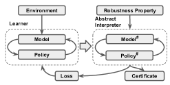
Figure 1: Schematic of Carol

Now we present the Carol framework. The framework (Figure 1) has two key components: a model-based learner and an abstract interpreter. During each training round, the learner maintains a model of the environment dynamics and a policy. These are sent to the abstract interpreter, which calculates a lower bound on the abstract reward. The lower bound is used to compute a differentiable loss the learner uses in the next iteration of learning. At convergence, the abstract trace computed during abstract interpretation is returned as a certificate of robustness.

Abstract Interpretation in Carol. Now we describe the abstract interpreter in Carol in more detail. Recall that our definition of robustness compares the expected reward of the original policy to the expected reward of the policy under an adversarial perturbation. As a result, our verifier is designed to reason about the worst-case reward under adversarial perturbations, while considering average-case behavior for stochastic policies and environments. Algorithm 1 finds a lower bound on this worst-case expected reward using abstract interpretation to overapproximate the adversary’s possible behaviors along with sampling to approximate the average-case behavior of the policy and environment. We denote this lower bound from Algorithm 1 as worst-case accumulative reward (Wcar), which is also used to measure the certified performance in our evaluation.

In more detail, Algorithm 1 proceeds by sampling a starting state $s_{0}\sim\mathcal{S}_{0}$. Then in Algorithm 2 for each time step, we find an overapproximation $s_{\text{obs}_{i}}^{\#}$ which includes all of the possible ways the adversary may perturb $s_{i}$. Based on this approximation, we sample a new approximation from the policy $\pi$. Intuitively, this may be done by using a policy $\pi$ whose randomness does not depend on the current state of the system. More formally, $\pi(a\mid s)=\mu_{\pi}(s)+f_{\pi}(a)$ where $f_{\pi}(a)$ is a distribution with zero mean which is independent of $s$. Then $a_{i}^{\#}$ may be computed as $\mu_{\pi}(s_{\text{obs}_{i}}^{\#})+\alpha(\{e\})$ where $e\sim f_{\pi}(a)$. Once the abstract action is computed, we may find the new (abstract) state and reward using the environment model $E$. The model is assumed to satisfy a PAC-style bound, i.e., there exist $\delta_{E}$ and $\varepsilon_{E}$ such that with probability at least $1-\delta_{E}$, $\|E(s,a)-P(s,a)\|\leq\varepsilon_{E}$. The values of $\delta_{E}$ and $\varepsilon_{E}$ can be measured during model construction.

One way to understand Algorithm 1 is to consider pairs of abstract and concrete trajectories in which the randomness is resolved in the same way. Specifically, if $\pi(a\mid s)=\mu_{\pi}(s)+f_{\pi}(a)$ and $E(s^{\prime}\mid s,a)=\mu(s,a)+f_{E}(s^{\prime})$, the initial state $s_{0}$ combined with the sequence of values $e_{i}\sim f_{\pi}(a)$ and $e^{\prime}_{i}\sim f_{E}(s^{\prime})$ for $0\leq i\leq T$ uniquely determine a trajectory. For a given set of values, the reward bound $\inf\beta(R_{\text{min}_{t}}^{\#})$ represents the worst-case reward under any adversary for a particular resolution of the randomness in the environment and the policy. The outer loop of Algorithm 1 approximates the expectation over these different random values by sampling. Theorem 1 in Section 5 shows formally that with high probability, Algorithm 1 gives a lower bound on the true adversarial reward.

Algorithm 1 Worst-Case Accumulative Reward (Wcar)

1:  Input: policy $\pi$, model $E$

2:  Output: worst case reward of $\pi$ under any adversary

3:  for $t$ from 1 to $N$ do

4:     Sample an initial state $s_{0}\sim\mathcal{S}_{0}$

5:     Get the worst case reward $R_{\text{min}_{t}}$ using Algorithm 2 over horizon $T$ starting from $s_{0}$

6:  end for

7:  return $\frac{1}{N}\sum_{t=1}^{N}R_{\text{min}_{t}}$

Algorithm 2 Worst-case rollout under adversarial perturbation

1:  Input: Initial state $s_{0}$, rollout horizon $T$

2:  Output: Worst-case reward of $\pi$ starting from $s_{0}$ over one random trajectory

3:  Abstract the initial state and reward: ${s_{\text{original}}}_{0}^{\#}\leftarrow\alpha(\{s_{0}\}),\quad{R_{\text{min}_{t}}^{\#}}_{i}\leftarrow\alpha\left(\{0\}\right)$

4:  for $i$ from 1 to $T$ do

5:     Abstract over possible perturbations: ${s_{\text{obs}}^{\#}}_{i}\leftarrow B({s_{\text{original}}^{\#}}_{i})$

6:     Calculate symbolic predicted actions: $a_{i}^{\#}\leftarrow\pi({s_{\text{obs}}^{\#}}_{i})$

7:     Calculate symbolic next-step states and rewards: ${s_{\text{original}}^{\#}}_{i+1},r^{\#}_{i}\leftarrow E_{\theta}({s_{\text{original}}^{\#}}_{i},a^{\#}_{i})+\alpha(\{x\mid\|x\|\leq\varepsilon_{E}\})$

8:     Update worst-case reward: ${R_{\text{min}}^{\#}}_{t}\leftarrow{R_{\text{min}}^{\#}}_{t}+r^{\#}_{i}$

9:  end for

10:  return $\inf\beta({R_{\text{min}}^{\#}}_{t})$

Algorithm 3 Certifiably Robust Reinforcement Learning

1:  Initialize a random policy $\pi_{\psi}$, random environment model $E_{\theta}$, and empty model dataset $\mathcal{D}_{\text{model}}$.

2:  Initialize an environment dataset $\mathcal{D}_{\text{env}}$ by unrolling trajectories under a random policy.

3:  for $N$ epochs do

4:     Train model $E_{\theta}$ on $\mathcal{D}_{\text{env}}$ via maximum likelihood

5:     Unroll $M$ trajectories int he model under $\pi_{\psi}$; add to $\mathcal{D_{\text{model}}}$

6:     Take action in environment according to $\pi_{\psi}$; add to $\mathcal{D_{\text{env}}}$

7:     for $G$ gradient updates do

8:        Calculate normal policy loss $L^{\text{normal}}(\pi_{\psi},\mathcal{D_{\text{model}}})$ as in MBPO [17]

9:        Sample $\langle s_{t},a_{t},s_{t+1},r_{t}\rangle$ uniformly from $\mathcal{D}_{\text{model}}$

10:        Rollout $\pi$ starting from $s_{t}$ under $E_{\theta}$ for $T_{\text{train}}$ steps and compute the total reward $R^{o}$

11:        Compute the worst-case reward $R_{\text{min}}$ using Algorithm 2 over horizon $T_{\text{train}}$.

12:        Compute the robustness loss $L^{\text{symbolic}}(\pi_{\psi},E_{\theta})\leftarrow R^{o}-R_{\text{min}}$

13:        Update policy parameters: $\psi\leftarrow\psi-\alpha\nabla_{\psi}(L^{\text{normal}}(\pi_{\psi},\mathcal{D}_{\text{model}})+\lambda(L^{\text{symbolic}}(\pi_{\psi},E_{\theta})-\Delta))$

14:        Update Lagrange multiplier: $\lambda\leftarrow\max(0,\lambda+\alpha^{\prime}(L^{\text{symbolic}}(\pi_{\psi},E_{\theta})-\Delta))$

15:     end for

16:     Unroll $n$ trajectories in the true environment under $\pi_{\psi}$; add to $\mathcal{D}_{\text{env}}$

17:  end for

Learning in Carol. Now we discuss how to learn a policy and environment model which may be proven robust by Algorithm 1. At a high level, Algorithm 3 works by introducing a symbolic loss term $L^{\text{symbolic}}_{\psi}$ which measures the robustness of the policy. Because robustness is a constrained optimization problem, we use this symbolic loss with a Lagrange multiplier in an alternating gradient descent scheme to find the optimal robust policy. Formally, for a given environment model $E$, the inner loop in Algorithm 3 solves the optimization problem

$$\operatorname*{arg\,min}_{\psi}L^{\text{normal}}(\pi_{\psi},\mathcal{D}_{\text{model}})\quad\text{s.t.}\quad L^{\text{symbolic}}(\pi,E)\leq\Delta$$

via the Lagrangian $\operatorname*{arg\,min}_{\psi}\max_{\lambda\geq 0}L^{\text{normal}}(\pi_{\psi},\mathcal{D}_{\text{model}})+\lambda(L^{\text{symbolic}}(\pi,E)-\Delta).$ We ensure that solving this problem solves the certifiable robustness problem by enforcing the following conditions: (i) $E$ accurately models the environment and (ii) $L^{\text{symbolic}}(\pi,E)$ measures the “provable robustness” of $\pi$. Condition (i) is handled by alternating model updates with policy updates, in the style of Dyna [35], so we will focus on condition (ii).

The computation of $L^{\text{symbolic}}$ uses the same underlying abstract rollouts (Algorithm 2) as the verifier described in Algorithm 1. Once again, this algorithm estimates the reward achieved by a policy under worst-case adversarial perturbations but average-case policy actions and environment transitions. We then define the robustness loss as the difference between the nominal loss $R^{o}$ and the provable lower bound on the worst-case loss $R_{\text{min}}$. Now as long as $L^{\text{symbolic}}<\Delta$, we satisfy the definition of robustness given in Section 3 for that specific trace. Repeating these gradient updates gives an approximation of the average-case behavior which is considered in Algorithm 1.

5 Theoretical Analysis

Now we explore some key theoretical properties of Carol. Proofs are deferred to Appendix B.

Theorem 1.

Assume the environment transition distribution is $P(s^{\prime}\mid s,a)=\mathcal{N}(\mu_{P}(s,a),{\bm{\Sigma}}_{P})$ and the environment model is $E(s^{\prime}\mid s,a)=\mathcal{N}(\mu_{E}(s,a),{\bm{\Sigma}}_{E})$ with ${\bm{\Sigma}}_{P},{\bm{\Sigma}}_{E}$ diagonal. Further, we assume that the model satisfies a PAC-style guarantee: for any state $s$, action $a$, and $\epsilon\in\mathcal{S}$, $|(\mu_{P}(s,a)+{\bm{\Sigma}}_{P}^{1/2}\epsilon)-(\mu_{E}(s,a)+{\bm{\Sigma}}_{E}^{1/2}\epsilon)|\leq\varepsilon_{E}$ with probability at least $1-\delta_{E}$. For any policy $\pi$, let the result of Algorithm 1 be $\hat{R}^{\#}$ and let the reward of $\pi$ under the optimal adversary $\nu^{*}$ be $R$. Then for any $\delta>0$ with probability at least $1-\delta$, we have

$$R\geq \hat{R}^{\#}-\frac{1}{\sqrt{\delta}}\sqrt{\frac{\mathrm{Var}\left[R^{\#}\right]}{N}}-\left(1-\left(1-\delta_{E}\right)^{T}\right)C.$$

where $C$ is a constant (see Appendix B for details of $C$).

Theorem 1 shows that our checker is a valid (probabilistic) proof strategy for determining if a policy is robust. That is, if we use Algorithm 1 to measure the reward of a policy under perturbation, the result is a lower bound of the true worst-case reward (minus a constant) with high probability, assuming an accurate environment model. The bound in Theorem 1 gives some interesting insights. First, the bound grows as $\delta$ shrinks, so we pay the price of a looser bound as we consider higher confidence levels. Second, the bound depends on the variance of the abstract reward and the number of samples in an intuitive way — higher variance makes it harder to measure the true reward, and more samples make the bound tighter. Third, as $\delta_{E}$ increases, the last term of the bound grows, indicating that a less accurate environment model leads to a looser bound. Finally, the bound grows with $T$, indicating that over longer time horizons, our reward measurement gets less accurate. This is consistent with the intuition that the environment model may drift away from the true environment over long rollouts.

Theorem 2.

Algorithm 3 converges to a policy $\pi$ which is robust and verifiable by Algorithm 1.

Intuitively, the theorem shows that Algorithm 3 solves the certifiable robustness problem, i.e., it converges to a policy that passes the check by Algorithm 1. The proof is straightforward because Algorithm 3 is a standard primal-dual approach to solve the constrained optimization problem outlined in Equation 1 [25].

6 Evaluation

We study the following experimental questions:

1. Can Carol learn policies with nontrivial certified reward bounds?

2. Do the certified bounds for Carol beat those for other (non-certified) robust RL methods?

3. How is Carol’s performance on empirical adversarial inputs?

4. How does Carol’s model-based training approach affect performance?

Environments and Setup. Our experiments consider $l_{\infty}$-norms perturbation of the state with radius $\epsilon$: $B_{p}(s,\epsilon):=\{s^{\prime}|\|s^{\prime}-s\|\leq\epsilon\}$. We implement Carol on top of the MBPO [17] model-based RL algorithm using the implementation from [27]. For training, we use Interval Bound Propagation (IBP) [15] as a scalable abstract interpretation mechanism to compute the layer-wise bounds for the neural networks, where all the abstract states are represented as intervals per dimension. More details of the abstract transition are omitted to Appendix E. During the evaluation, we use CROWN [41], a more computationally expensive but tighter bound propagation method based on IBP. During training, we use a $\epsilon$-schedule [15, 42] to slowly increase the $\epsilon_{t}$ at each epoch within the perturbation budget until reaching $\epsilon$. Note that the policies take action stochastically during training, but we set them to be deterministic during evaluation.

We experiment on four MuJoCo environments in OpenAI Gym [2]. For Carol, we use the same hyperparameters for the base RL algorithms as in [27] without further tuning. Specifically, we do not use an ensemble of dynamics models. Instead, we use a single dynamic model, which is the case when the ensemble is of size 1. We use Gaussian distribution as the independent noise distribution, $f_{\pi}(a),f_{E}(s^{\prime})$ for both policy and model in the experiments. Concretely, the output of our policies are the parameters $\mu_{\pi}$, ${\bm{\Sigma}}_{\pi}$ of a Gaussian, with ${\bm{\Sigma}}_{\pi}$ being diagonal and independent of input state $s$. For the model, the output are the parameters $\mu_{E}$, ${\bm{\Sigma}}_{E}$ of a Gaussian, with ${\bm{\Sigma}}_{E}$ being diagonal and independent of input $s,a$. The model error $\varepsilon_{E}$ is measured and considered following Algorithm 2. We defer the detailed descriptions of the model error and its construction details to Section C.2.

We compare Carol with the following methods: (1) MBPO [17], our base RL algorithm. (2) SA-PPO [42], a robust RL algorithm bounding per-step action distance. (3) RADIAL-PPO [26], a robust RL algorithm using lower bound PPO loss to update the policy. (4) Carol-Separate Sampler(Carol-SS), an ablation of Carol. In Carol, we update the policy loss $L^{\text{normal}}$ with the data sampled from the rollout between the learned model and the policy. While in Carol-SS, the data for $L^{\text{normal}}$ is sampled from the rollout between the environment and the policy. The $\epsilon_{\text{train}}$ is 0.075, 0.05, 0.075, 0.05 for Hopper, Walker2d, HalfCheetah, and Ant for Carol, Carol-SS, SA-PPO, and RADIAL-PPO in this section for consistency with baselines. Detailed training setup are available in Section C.1.

Evaluation. We evaluate the performance of policies with two metrics: (i). Wcar, which was formally defined in Algorithm 1 for certified performance. (ii). total reward under MAD attacks [42] for empirical performance.

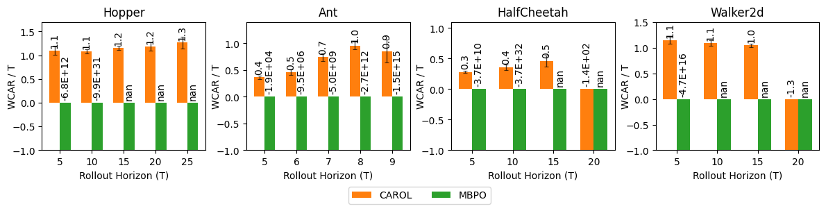
Figure 2: Certified performance of policies $\pi$ with the learned-together model, $E$. To have a fair comparison across different horizons, we quantify the certified performance by $\text{{Wcar}}/T$, where Wcar is formally defined in Algorithm 1 and $T$ is the rollout horizon in Algorithm 2. Each bar is an average of 25 starting states. nan denotes not a number, which means that ($\pi,E$) is not certifiable by a third-party verifier [41]. We use negative infinity to exhibit nan’s value. A higher value indicates a better certified worst-case performance. The results are based on $\varepsilon_{E}$ with a $1-\delta_{E}$ of $0.9$.

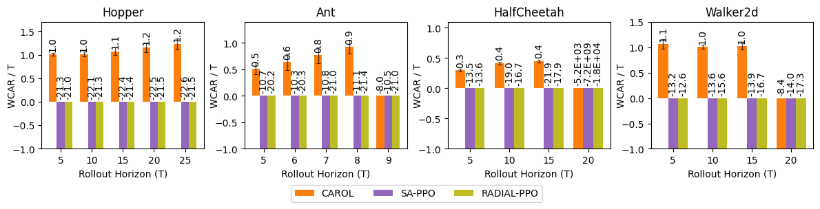
Figure 3: Certified performance of policies $\pi$ under a set of separately learned models, $\{E_{i}\}$. Each bar averages the learned policies on each $E_{i}$ of 25 starting states. The results are based on $\varepsilon_{E}$ with a $1-\delta_{E}$ of $0.9$.

RQ1: Certified Performance with Learned-together Certificate. After training, we get a policy, $\pi$, and an environment model, $E$, trained with the policy. Then, we evaluate the Wcar following Algorithm 1 with $\pi$ and $E$. Note that we use an $\epsilon_{\text{test}}=\frac{1}{255}$ for the evaluation of provability as certifying over long-horizon traces of neural network models tightly is a challenging task for abstract interpreters due to accumulated approximation error. The proof becomes more challenging as the horizon increases, primarily due to the consideration of the adversary’s behavior in the most unfavorable scenarios at each step, and the step-wise impact from the worst-case adversary accumulates. We vary the certified horizon under the $\epsilon_{\text{test}}$ to exhibit the certified performance.

Figure 2 exhibits the certified performance of Carol. Both Carol and MBPO are evaluated with the model trained together. We are able to train a policy with better certified accumulative reward under the worst attacks compared to the base algorithm, MBPO, which does not use the regularization $L^{\text{symbolic}}$. As the time horizon increases, it becomes harder to certify the accumulative reward. For example, in Ant and HalfCheetah, Carol is not able to give a good certified performance when the horizon reaches $10$ and $20$ respectively because of the accumulative influence from the worst-case attack and the overapproximation from the abstract interpreter. We also highlight that Ant is a challenging task for certification due to the high-dimensional state space.

RQ2: Comparison of Certified Performance with Other Methods. We compare Carol with two robust RL methods, SA-PPO [42] and RADIAL-PPO [26], which both bound the per-step performance of the policy during training. SA-PPO bounds the per-step action deviation under perturbation, and RADIAL-PPO bounds the one-step loss under perturbation. To have a fair comparison of the certified performance of policies and alleviate the impact from model error bias across methods, we separately train 5 additional environment models, $\{E_{i}\}$, with the trajectory datasets unrolled from 5 additional random policies and the environment. Details are deferred to Section C.2. We truncate Carol by extracting the policies from training and certify them with these separately trained environment models. This setting is not completely inline with Carol’s learned certificate and verification (see RQ1) but is designed for a fair comparison across policies.

As shown in Figure 3, the Carol’s certified performance with separately trained models is slightly worse yet comparable to its performance when using learned-together certificates. Compared with non-certified RL policies, Carol consistently exhibits better certifiable performance. It is worth noting that Carol is able to provide worst-case rewards over time for benchmarks aligning with the reward mechanisms used in these environments. We show the abstract trace lower bound ($R_{\text{min}}$) sampled from trajectories in Appendix D. These results demonstrate that Carol is able to provide reasonable certified performance, while the other methods, which are not specifically designed for worst-case accumulative reward certification, struggle to attain the same goal.

		Nominal	Attack (MAD)
Environment	Model	$\epsilon=0$	$\epsilon=\epsilon_{\text{train}}$
Hopper ($\epsilon_{\text{train}}=0.075$)	MBPO	3246.0$\pm$76.1	2874.2$\pm$203.4
	SA-PPO	3423.9$\pm$164.2	3213.8$\pm$284.8
	RADIAL-PPO	3547.0$\pm$166.9	3100.3$\pm$368.3
	CAROL	3290.1$\pm$104.9	3201.4$\pm$100.5
Ant ($\epsilon_{\text{train}}=0.05$)	MBPO	4051.9$\pm$526.2	406.2$\pm$83.5
	SA-PPO	5368.8$\pm$96.4	5327.4$\pm$112.7
	RADIAL-PPO	4694.1$\pm$219.5	4478.9$\pm$232.8
	CAROL	5696.6$\pm$277.9	5362.2$\pm$242.8
HalfCheetah ($\epsilon_{\text{train}}=0.075$)	MBPO	7706.3$\pm$710.1	2314.6$\pm$566.7
	SA-PPO	3193.9$\pm$650.7	3231.6$\pm$659.9
	RADIAL-PPO	3686.5$\pm$439.2	3409.6$\pm$683.9
	CAROL	5821.5$\pm$2401.9	3961.6$\pm$899.5
Walker2d ($\epsilon_{\text{train}}=0.05$)	MBPO	3815.6$\pm$211.9	3616.5$\pm$228.2
	SA-PPO	4271.7$\pm$222.2	4444.4$\pm$286.0
	RADIAL-PPO	2935.1$\pm$272.1	3022.6$\pm$381.7
	CAROL	3784.4$\pm$329.1	3774.3$\pm$260.3

Table 2: Average episodic reward $\pm$ standard deviation over 100 episodes on three baselines and Carol. We show natural rewards (under no attack) and rewards under adversarial attacks. The best results over all methods are in bold.

RQ3: Comparison of Empirical Performance with Other Methods. Usually, there is a trade-off between certified robustness and empirical robustness. One can get good provability but may sacrifice empirical rewards. We show that policy from our algorithm shows comparable natural rewards (without attack) and adversarial rewards compared with other methods. In Table 2, we show results on 4 environments and comparison with MBPO, SA-PPO, and RADIAL-PPO. The policies are the same ones evaluated for RQ1 and RQ2. For each environment, we compare the performance under MAD attacks [42]. Carol outperforms other methods on Ant and HalfCheetah under attacks when the base algorithm, MBPO, is extremely not robust. For Hopper, Carol has comparable adversarial rewards with the best methods. Carol’s reward is worse on Walker2d though still reasonable.

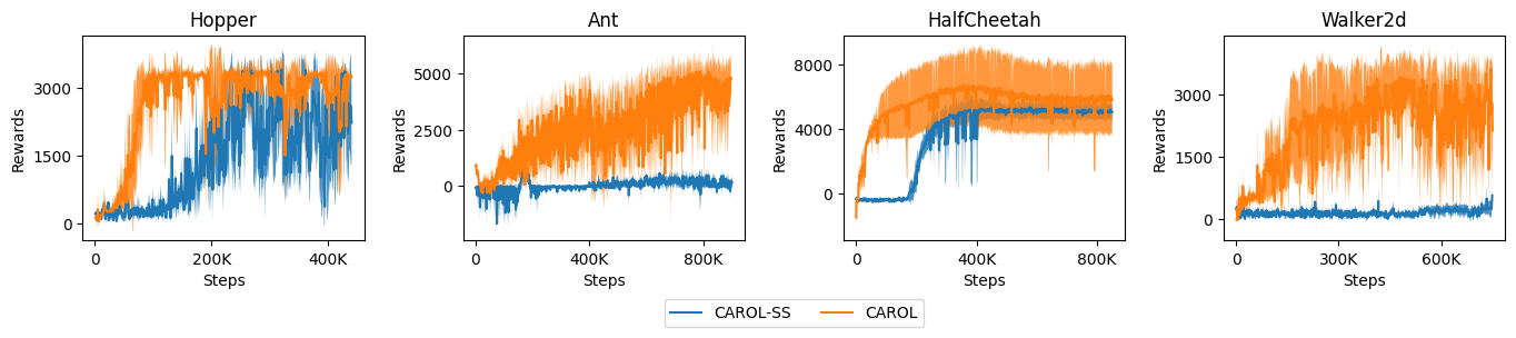
Figure 4: Training Curves of Carol and Carol-SS. The solid lines in the graph show the average natural rewards of five training trials, and the shaded areas represent the standard deviation among those trials.

RQ4: Impact of Model-Based Training. In this part, we investigate the impact of our design choices for $L^{\text{normal}}$ on performance. We compare our framework, Carol, with an ablation of it, Carol-SS, to understand how rollout with the learned model for $L^{\text{normal}}$ matters in Carol. We present a comparison of performance during training, as shown in Figure 4. In the implementation, we set a smoother $\epsilon$-schedule for Carol-SS by allowing Carol-SS to take longer steps from $\epsilon=0$ to the target $\epsilon$. These results show that Carol converges much faster while achieving a comparable or better final performance due to the benefits of the sample efficiency of MBRL. Additionally, the consistency between the rollout datasets for $L^{\text{normal}}$ and the ones for $L^{\text{symbolic}}$ also leads to a better natural reward at convergence in training.

7 Related Work

Adversarial RL. Adversarial attacks on RL systems have been extensively studied. Specific attacks include adversarial perturbations on agents’ observations or actions [16, 20, 36], adversarial disturbance forces to the system [28], and other adversarial policies in a multiagent setting [14]. Most recently, [43] and [34] consider an optimal adversary and propose methods to train agents together with a learned adversary in an online way to achieve a better adversarial reward.

Robust RL and Certifiable Robustness in RL. Multiple robust training methods have been applied to deep RL. Mankowitz et al. [22] explore a broader adversarial setting related to model disturbances and model uncertainty. Fischer et al. [13] leverage additional student networks to help the robust Q learning, and Everett et al. [12] enhance an agent’s robustness during testing time by computing the lower bound of each action’s Q value at each step. Zhang et al. [42] and Oikarinen et al. [26] leverage a bound propagation technique in a loss regularizer to encourage the agent to either follow its original actions or optimize over a loss lower bound. While these efforts achieve robustness by deterministic certification techniques for neural networks [15, 39], they mainly focus on the step-wise certification and are not able to give robustness certification if the impact from attacks accumulates across multiple steps. Carol differs from these papers by offering certified robustness for the aggregate reward in an episode. We know of only two recent efforts that study robustness certification for cumulative rewards. The first, by Wu et al. [38], gives a framework for certification rather than certified learning. The second, by Kumar et al. [18], proposes a certified learning algorithm under the assumption that the adversarial perturbation is smoothed using random noise. The attack model here is weaker than the adversarial model assumed by Carol and most other work on adversarial learning.

Certified RL. Safe control with learned certificates is an active field [10]. A few efforts in this space have considered controllers discovered through RL. Many works use a given certificate with strong control-theoretic priors to constrain the actions of an RL agent [4, 19, 5] or assume the full knowledge of the environment to yield the certificate during the training of an agent [40]. Chow et al. [7, 6] attempt to derive certificates from the structure of the constrained Markov decision process [1] for the safe control problems. Chang et al. [3] incorporate Lyapunov methods in deep RL to learn a neural Lyapunov critic function to improve the stability of an RL agent. We differ from this work by focusing on adversarial robustness rather than stability.

8 Discussion

We have presented Carol, the first RL framework with certifiable episode-level robustness guarantees. Our approach is based on a new combination of model-based RL and abstract interpretation. We have given a theoretical analysis to justify the approach and validated it empirically in four challenging continuous control tasks.

A key challenge in Carol is that our abstract interpreter may not be sufficiently precise, and attempts to increase precision may compromise scalability. Future research should work to address this issue with more accurate and scalable verification techniques. Also, as seen in Figure 4, there is variance in the results due to the use of a single dynamics model. To address this issue, future work should explore ways to incorporate certificates across ensembles of models. Moreover, because abstract interpretation of probabilistic systems is difficult, our approach assumes that the randomness in the environment transitions is state-independent. Future work should try to eliminate this assumption through abstract interpreters tailored to probabilistic systems. Finally, we focus on the state-adversarial setting, which of practical applications. However, there are broader adversarial settings encompassing model disturbances and model uncertainty. Exploring these areas within the context of certified learning is also an interesting future direction. A broader discussion of limitations appears in Appendix F.

Appendix A Symbols

We give a summary of the symbols used in this paper below.

Definition	Symbol/Notation
Policy	$\pi_{\psi},\pi$
Model of the environment	$E_{\theta},E$
Environment transition	$P$
Parameters (mean, covariance) for Gaussian distribution for environment, model, and policy	$\mu_{P},{\bm{\Sigma}}_{P},\mu_{E},{\bm{\Sigma}}_{E},\mu_{\pi},{\bm{\Sigma}}_{\pi}$
Distribution representing noise for environment, model, and policy	$f_{P},f_{E},f_{\pi}$
Adversary	$\nu$
Regular policy loss	$L^{\text{normal}}$
Robustness loss	$L^{\text{symbolic}}$
Lipschitz constants for the environment model and policy mean	$L_{E}$, $L_{\pi}$
Model error	$\varepsilon_{E}$
PAC bound probability	$\delta_{E}$
Abstract lifts	$\cdot^{\#}$
Abstraction	$\alpha$
Concretization	$\beta$
Horizon for training and testing	$T$, $T_{\text{train}}$, $T_{\text{test}}$
Disturbance for training and testing	$\epsilon$, $\epsilon_{\text{train}}$, $\epsilon_{\text{test}}$

Appendix B Proofs

In this section we present proofs of the theorems from Section 5.

Assumption 3.

The horizon of the MDP is bounded by $T$.

Assumption 4.

The environment transition distribution has the form $P\left(s^{\prime}\mid s,a\right)=\mathcal{N}\left(\mu_{P}\left(s,a\right),{\bm{\Sigma}}_{P}\right)$ with ${\bm{\Sigma}}_{P}$ diagonal and the environment model $E$ has the form $E\left(s^{\prime}\mid s,a\right)=\mathcal{N}\left(\mu_{E}(s,a),{\bm{\Sigma}}_{E}\right)$ with ${\bm{\Sigma}}_{E}$ diagonal.

Assumption 5.

There exist values $\varepsilon_{E}$ and $\delta_{E}$ such that for all $s,a$ and for any fixed $e$ with probability at least $1-\delta_{E}$, $\left\|\left(\mu_{P}\left(s,a\right)+{\bm{\Sigma}}_{P}^{1/2}e\right)-\left(\mu_{E}\left(s,a\right)+{\bm{\Sigma}}_{E}^{1/2}e\right)\right\|\leq\varepsilon_{E}$. Further, there exists some $d_{E}$ such that for all $s,a$, $\left\|\left(\mu_{P}\left(s,a\right)+{\bm{\Sigma}}_{P}^{1/2}e\right)-\left(\mu_{E}\left(s,a\right)+{\bm{\Sigma}}_{E}^{1/2}e\right)\right\|\leq d_{E}$.

Assumption 6.

The environment model mean function $\mu_{E}\left(s,a\right)$ is $L_{E}$-Lipschitz continuous, the immediate reward function $r\left(s,a\right)$ is $L_{r}$-Lipschitz continuous, and the policy mean $\mu_{\pi}\left(s\right)$ is $L_{\pi}$-Lipschitz continuous.

Assumption 7.

For all $s\in\mathcal{S}$, we have $s\in B\left(s\right)$. That is, the adversary may choose not to perturb any state.

Theorem 1.

For any policy $\pi$, let the result of Algorithm 1 be $\hat{R}^{\#}$, let $\nu^{*}$ be the optimal adversary (i.e., for all $\nu\in\mathbb{A}_{B}$, $R\left(\pi\circ\nu^{*}\right)\leq R\left(\pi\circ\nu\right)$), and let the reward of $\pi\circ\nu^{*}$ be $R$. Then for any $\delta>0$ with probability at least $1-\delta$, we have

$$R\geq\hat{R}^{\#}\left(\tau\right)-\frac{1}{\sqrt{\delta}}\sqrt{\frac{\mathrm{Var}\left[R^{\#}\right]}{N}}-\left(1-\left(1-\delta_{E}\right)^{T}\right)L_{r}(1+L_{\pi})d_{E}\frac{\left(L_{E}L_{\pi}\right)^{T}+\left(1-L_{E}L_{\pi}\right)T-1}{\left(1-L_{E}L_{\pi}\right)^{2}}.$$

Proof.

Recall that the environment transition $P$ and policy $\pi$ are assumed to be separable, i.e., $P\left(s^{\prime}\mid s,a\right)=\mu_{P}\left(s,a\right)+f_{P}\left(s^{\prime}\right)$ and $\pi\left(a\mid s\right)=\mu_{\pi}\left(s\right)+f_{\pi}\left(a\right)$ with $\mu_{P}$ and $\mu_{\pi}$ deterministic. As a result, a trajectory under policy $\pi\circ\nu^{*}$ may be written $\tau=s_{0},a_{0},s_{1},a_{1},\ldots,s_{n},a_{n}$ where $s_{0}\sim\mathcal{S}_{0}$, each $a_{i}=\mu_{\pi}\left(\nu^{*}\left(s_{i}\right)\right)+e^{\pi}_{i}$ for $e^{\pi}_{i}\sim f_{\pi}\left(a\right)$, and each $s_{i}=\mu_{P}\left(s_{i-1},a_{i-1}\right)+e^{P}_{i}$ for $e^{P}_{i}\sim f_{P}\left(s^{\prime}\right)$. By Assumption 4, we know that $e^{P}_{i}\sim\mathcal{N}\left({\bm{0}},{\bm{\Sigma}}_{P}\right)$ so that $e^{P}_{i}={\bm{\Sigma}}_{P}^{1/2}e_{i}$ where $e_{i}\sim\mathcal{N}\left(0,{\bm{I}}\right)$. In particular, because each trajectory $\tau$ is uniquely determined by $s_{0},\{e^{\pi}_{i}\}_{i=0}^{n},\{e_{i}\}_{i=1}^{n}$, we can write the reward of $\pi\circ\nu^{*}$ as

$$R\left(\pi\circ\nu^{*}\right)=\mathop{\mathbb{E}}_{s_{0}\sim\mathcal{S}_{0},\left\{e^{\pi}_{i}\sim f_{\pi}\left(a\right)\right\}_{i=0}^{n},\left\{e_{i}\sim\mathcal{N}\left({\bm{0}},{\bm{I}}\right)\right\}_{i=1}^{n}}R\left(\tau\right)$$

Because this expectation ranges over the values of $s_{0},\left\{e^{\pi}_{i}\right\}_{i=0}^{n},\left\{e_{i}\right\}_{i=1}^{n}$, we will proceed by considering pairs of abstract and concrete trajectories unrolled with the same starting state and noise terms.

To do this, we analyze Algorithm 2 for some fixed $s_{0},\left\{e^{\pi}_{i}\right\}_{i=0}^{n},\left\{e_{i}\right\}_{i=1}^{n}$. Let $e^{E}_{i}={\bm{\Sigma}}_{E}^{1/2}e_{i}$. That is, given the same underlying sample from $\mathcal{N}\left(0,{\bm{I}}\right)$, $e^{P}_{i}$ is the noise in the true environment while $e^{E}_{i}$ is the noise in the modeled environment. We show by induction that for all $i$, $s_{i}\in\beta\left(s_{\text{original}_{i}}^{\#}\right)$ with probability at least $\left(1-\delta_{E}\right)^{i}$. Note that, because abstract interpretation is sound, $s_{0}\in\beta\left(s_{\text{original}_{0}}^{\#}\right)$. Additionally, for all $i$ if $s_{i}\in\beta\left(s_{\text{original}_{i}}^{\#}\right)$ then $\nu^{*}\left(s_{i}\right)\in\beta\left(s_{\text{obs}_{i}}^{\#}\right)$. Moreover, since $e^{\pi}_{i}$ is fixed, we have

$$\pi\left(s_{\text{obs}_{i}}^{\#}\right)=\mu_{\pi}\left(s_{\text{obs}_{i}}^{\#}\right)+e^{\pi}_{i}$$

so that $\pi\left(\nu^{*}\left(s\right)\right)\in\beta\left(a_{i}^{\#}\right)$. Similarly, because $e^{E}_{i}$ is fixed, let $\Delta_{E}=\alpha\left(\left\{x\mid\left\|x\right\|\leq\varepsilon_{E}\right\}\right)$ and we have

$$E\left(s_{\text{original}_{i}}^{\#},a_{i}^{\#}\right)+\Delta_{E}=\mu_{E}\left(s_{\text{original}_{i}}^{\#},a_{i}^{\#}\right)+e^{E}_{i}+\Delta_{E}.$$

By the induction hypothesis, we know that $s_{i-1}\in\beta\left(s_{\text{original}_{i-1}}^{\#}\right)$ with probability at least $\left(1-\delta_{E}\right)^{i-1}$ and therefore $a_{i-1}\in\beta\left(a_{i-1}^{\#}\right)$. By Assumption 5, we have that $\left\|\left(\mu_{P}\left(s,a\right)+e^{P}_{i}\right)-\left(\mu_{E}\left(s,a\right)+e^{E}_{i}\right)\right\|<\varepsilon_{E}$ with probability at least $1-\delta_{E}$. In particular, $\left(\mu_{P}\left(s,a\right)+\varepsilon^{P}_{i}\right)-\left(\mu_{E}\left(s,a\right)+\varepsilon^{E}_{i}\right)\in\Delta_{E}$, so that $\mu_{P}\left(s,a\right)+e^{P}_{i}\in\beta\left(E\left(s_{\text{original}_{i}}^{\#},a_{i}^{\#}\right)+\Delta_{E}\right)$. Then with probability at least $1-\delta_{E}$, if $s_{i-1}\in\beta\left(s_{\text{original}_{i-1}}^{\#}\right)$ then $s_{i}\in\beta\left(s_{\text{original}_{i}}^{\#}\right)$. As a result, $s_{i}\in\beta\left(s_{\text{original}_{i}}^{\#}\right)$ with probability at least $\left(1-\delta_{E}\right)^{i}$. In particular, by Assumption 3, $n\leq T$ so that for a fixed $\tau$ defined by $s_{0},\left\{e^{\pi}_{i}\right\}_{i=0}^{n},\left\{e_{i}\right\}_{i=1}^{n}$, we have that with probability at least $\left(1-\delta_{E}\right)^{T}$, Algorithm 2 returns a lower bound on $R\left(\tau\right)$.

Now we consider the case where Algorithm 2 does not return a lower bound of $R\left(\tau\right)$. In this case, we show (again by induction) that for all $0\leq i\leq T$, there exists a point $s_{i}^{\prime}\in\beta\left(s_{\text{original}_{i}}^{\#}\right)$ such that

$$\left\|s_{i}-s_{i}^{\prime}\right\|\leq\sum_{j=0}^{i-1}\left(L_{E}L_{\pi}\right)^{j}d_{E}=d_{E}\left(\frac{1-\left(L_{E}L_{\pi}\right)^{i-1}}{1-L_{E}L_{\pi}}\right)$$

(when $\sum_{j=0}^{-1}\left(L_{E}L_{\pi}\right)^{j}d_{E}$ is taken to be zero). First, note that $s_{0}\in\beta\left(s_{\text{original}_{0}}^{\#}\right)$, so the base case is trivially true. Now by the induction hypothesis we have that there exists some $s_{i-1}^{\prime}\in\beta\left(s_{\text{original}_{i-1}}^{\#}\right)$ with $\left\|s_{i-1}-s_{i-1}^{\prime}\right\|\leq\sum_{j=0}^{i-2}\left(L_{E}L_{\pi}\right)^{j}d_{E}$. Notice that by Assumption 7, we also have $s_{i-1}^{\prime}\in\beta\left(s_{\text{obs}_{i-1}}^{\#}\right)$. Now because abstract interpretation is sound, we have that $\mu_{\pi}\left(s_{i-1}^{\prime}\right)+e^{\pi}_{i-1}\in\beta\left(a_{i-1}^{\#}\right)$ and by Assumption 6, $\|\mu_{\pi}\left(s_{i-1}\right)-\mu_{\pi}\left(s_{i-1}^{\prime}\right)\|\leq L_{\pi}\sum_{j=0}^{i-2}\left(L_{E}L_{\pi}\right)^{j}d_{E}$. Similarly, we have $\mu_{E}\left(s_{i-1}^{\prime},\mu_{\pi}\left(s_{i-1}^{\prime}\right)+e^{\pi}_{i-1}\right)+e^{E}_{i}\in\beta\left(s_{\text{original}_{i}}^{\#}\right)$, and $\left\|\mu_{E}\left(s_{i-1},\mu_{\pi}\left(s_{i-1}\right)+e^{\pi}_{i-1}\right)-\mu_{E}\left(s_{i-1}^{\prime},\mu_{\pi}\left(s_{i-1}^{\prime}\right)+e^{\pi}_{i-1}\right)\right\|\leq L_{E}L_{\pi}\sum_{j=0}^{i-2}\left(L_{E}L_{\pi}\right)^{j}d_{E}$. Let $\hat{s}_{i}=\mu_{E}\left(s_{i-1},\mu_{\pi}\left(s_{i-1}\right)+\varepsilon_{i-1}^{\pi}\right)+\varepsilon^{E}_{i}$. Then by Assumption 5, we have $\left\|\hat{s}_{i}-s_{i}\right\|\leq d_{E}$, so that in particular $\left\|s_{i}-\mu_{E}\left(s_{i-1}^{\prime},\mu_{\pi}\left(s_{i-1}^{\prime}\right)+e^{\pi}_{i-1}\right)+\varepsilon^{E}_{i}\right\|\leq d_{E}+L_{E}L_{\pi}\sum_{j=0}^{i-2}\left(L_{E}L_{\pi}\right)^{j}d_{E}$. Letting $s_{i}^{\prime}=\mu_{E}\left(s_{i-1}^{\prime},\mu_{\pi}\left(s_{i-1}^{\prime}\right)+e^{\pi}_{i-1}\right)+\varepsilon^{P}_{i}$, we have the desired result.

We use this result to bound the difference in reward between the abstract and concrete rollouts when Algorithm 2 does not return a lower bound. For each $i$, because $s_{i}^{\prime}\in\beta\left(s_{\text{original}_{i}}^{\#}\right)$ and $\mu_{\pi}\left(s_{i}^{\prime}\right)+e^{\pi}_{i}\in a_{i}^{\#}$, we define $r_{i}^{\prime}=r\left(s_{i}^{\prime},\mu_{\pi}\left(s_{i}^{\prime}\right)+e^{\pi}_{i}\right)$ and we know that $r^{\prime}\in r_{i}^{\#}$. Because $\left\|s_{i}-s_{i}^{\prime}\right\|\leq d_{E}\left(\frac{1-\left(L_{E}L_{\pi}\right)^{i-1}}{1-L_{E}L_{\pi}}\right)$ we have $\left\|a_{i}-a_{i}^{\prime}\right\|\leq L_{\pi}d_{E}\left(\frac{1-\left(L_{E}L_{\pi}\right)^{i-1}}{1-L_{E}L_{\pi}}\right)$ and $\left|r\left(s_{i},a_{i}\right)-r_{i}^{\prime}\right|\leq L_{r}(1+L_{\pi})d_{E}\left(\frac{1-\left(L_{E}L_{\pi}\right)^{i-1}}{1-L_{E}L_{\pi}}\right)$. In particular, let $R^{\prime}=\sum_{i}r_{i}^{\prime}$ and then

$$\left|R\left(\tau\right)-R^{\prime}\right| \leq\sum_{i=1}^{T}L_{r}(1+L_{\pi})d_{E}\left(\frac{1-\left(L_{E}L_{\pi}\right)^{i-1}}{1-L_{E}L_{\pi}}\right)$$

$$=L_{r}(1+L_{\pi})d_{E}\frac{\left(L_{E}L_{\pi}\right)^{T}+\left(1-L_{E}L_{\pi}\right)T-1}{\left(1-L_{E}L_{\pi}\right)^{2}}.$$

We now combine these two cases to bound the expected difference between the reward returned by Algorithm 2, denoted $R^{\#}\left(\tau\right)$, and the reward of $\tau$. Let $D=R^{\#}\left(\tau\right)-R\left(\tau\right)$ be a random variable representing this difference. Then with probability at least $\left(1-\delta_{E}\right)^{T}$, $D\leq 0$ and in all other cases (i.e., with probability no greater than $1-\left(1-\delta_{E}\right)^{T}$), $D\leq L_{R}(1+L_{\pi})d_{E}\frac{\left(L_{E}L_{\pi}\right)^{T}+\left(1-L_{E}L_{\pi}\right)T-1}{\left(1-L_{E}L_{\pi}\right)^{2}}$. In particular then,

$$\mathop{\mathbb{E}}\left[D\right]\leq\left(1-\left(1-\delta_{E}\right)^{T}\right)L_{r}(1+L_{\pi})d_{E}\frac{\left(L_{E}L_{\pi}\right)^{T}+\left(1-L_{E}L_{\pi}\right)T-1}{\left(1-L_{E}L_{\pi}\right)^{2}}.$$

By definition $\mathop{\mathbb{E}}\left[R^{\#}\left(\tau\right)\right]=\mathop{\mathbb{E}}\left[R\left(\tau\right)\right]+\mathop{\mathbb{E}}\left[D\right]$. Therefore, we have

$$\begin{split}\mathop{\mathbb{E}}\left[R\left(\tau\right)\right]&=\mathop{\mathbb{E}}\left[R^{\#}\left(\tau\right)\right]-\mathop{\mathbb{E}}\left[D\right]\geq\mathop{\mathbb{E}}\left[R^{\#}\left(\tau\right)\right]\\ &-\left(1-\left(1-\delta_{E}\right)^{T}\right)L_{r}(1+L_{\pi})d_{E}\frac{\left(L_{E}L_{\pi}\right)^{T}+\left(1-L_{E}L_{\pi}\right)T-1}{\left(1-L_{E}L_{\pi}\right)^{2}}.\end{split}$$ (2)

Algorithm 3 approximates $\mathop{\mathbb{E}}\left[R^{\#}\left(\tau\right)\right]$ by sampling $N$ values. Let $\hat{R}^{\#}\left(\tau\right)$ be the measured mean and recall $\mathop{\mathbb{E}}\left[\hat{R}^{\#}\left(\tau\right)\right]=\mathop{\mathbb{E}}\left[R^{\#}\left(\tau\right)\right]$ and $\mathrm{Var}\left[\hat{R}^{\#}\left(\tau\right)\right]=\mathrm{Var}\left[R^{\#}\left(\tau\right)\right]/N$. Then by Chebyshev’s inequality we have the for all $k>0$, $\mathrm{Pr}\left[\left|\hat{R}^{\#}\left(\tau\right)-\mathop{\mathbb{E}}\left[R^{\#}\left(\tau\right)\right]\right|\geq k\sqrt{\mathrm{Var}\left[\hat{R}^{\#}\left(\tau\right)\right]}\right]\leq 1/k^{2}$. Then in particular, with probability at least $1-1/k^{2}$,

$$\hat{R}^{\#}\left(\tau\right)-k\sqrt{\frac{\mathrm{Var}\left[R^{\#}\left(\tau\right)\right]}{N}}\leq R^{\#}\left(\tau\right).$$

Combining this with Equation 2 above and letting $k=1/\sqrt{\delta}$, we have with probability at least $1-\delta$,

$$\mathop{\mathbb{E}}\left[R\left(\tau\right)\right] \geq\hat{R}^{\#}\left(\tau\right)-\frac{1}{\sqrt{\delta}}\sqrt{\frac{\mathrm{Var}\left[R^{\#}\left(\tau\right)\right]}{N}}$$

$$-\left(1-\left(1-\delta_{E}\right)^{T}\right)L_{r}(1+L_{\pi})d_{E}\frac{\left(L_{E}L_{\pi}\right)^{T}+\left(1-L_{E}L_{\pi}\right)T-1}{\left(1-L_{E}L_{\pi}\right)^{2}}.$$

∎

While this paper focuses on continuous state and action spaces, we can extend our main theoretical result to discrete state and action spaces if the environment is deterministic. For this analysis, we maintain Assumptions 3 and 7, but we add a few new assumptions for the discrete setting.

Assumption 8.

The environment model $E$ is deterministic and $E(s,a)=P(s,a)$ with probability at least $1-\delta_{E}$.

Assumption 9.

The single-step reward for any state $s$ and action $a$ is bounded by $r_{\min}\leq r(s,a)\leq r_{\max}$.

Theorem 10.

For a deterministic policy $\pi$, let the result of Algorithm 1 be $\hat{R}^{\#}$, let $\nu^{*}$ be the optimal adversary, and let the reward of $\pi\circ\nu^{*}$ be $R$. Then for any $\delta$, with probability at least $1-\delta$,

$$R\geq\hat{R}^{\#}-\frac{1}{\sqrt{\delta}}\sqrt{\frac{\mathrm{Var}[R^{\#}]}{N}}-T(r_{\max}-r_{\min}).$$

Proof.

Consider a trajectory $\tau=s_{0},a_{0},s_{1},a_{1},\ldots,s_{n},a_{n}$ where $s_{0}\sim\mathcal{S}_{0}$, each $a_{i}=\pi(s_{i})$, and each $s_{i+1}=P(s_{i},a_{i})$. Note that because the dynamics of the environment and the policy are deterministic, the only randomness in the trajectory comes from sampling the initial state. Then $R(\pi\circ\nu^{*})=\mathbb{E}_{s_{0}\sim\mathcal{S}_{0}}R(\tau)$. Similar to the proof of Theorem 1, we proceed by considering pairs of abstract and concrete trajectories unrolled from the same starting state.

We show by induction that for all $i$, $s_{i}\in\beta\left(s_{\text{original}_{i}}^{\#}\right)$ with probability at least ${\left(1-\delta_{E}\right)}^{i}$. For the base case, note that because abstract interpretation is sound, $s_{0}\in\beta\left(s_{\text{original}_{0}}^{\#}\right)$. Additionally, for all $i$, if $s_{i}\in\beta\left(s_{\text{original}_{i}}^{\#}\right)$ then $\nu^{*}(s_{i})\in\beta\left(s_{\text{obs}_{i}}^{\#}\right)$ and $\pi(\nu^{*}(s_{i}))\in\beta\left(a_{i}^{\#}\right)$. From the induction hypothesis, we have $s_{i-1}\in\beta\left(s_{\text{original}_{i-1}}^{\#}\right)$ with probability at least $\left(1-\delta_{E}\right)^{i-1}$. By Assumption 8, we have $s_{i+1}=E(s_{i},a_{i})$ with probability at least $1-\delta_{E}$. Thus if $s_{i-1}\in\beta\left(s_{\text{original}_{i-1}}^{\#}\right)$ then with probability at least $1-\delta_{E}$ we know $s_{i}\in\beta\left(s_{\text{original}_{i}}^{\#}\right)$. Combined with the induction hypothesis, this implies that $s_{i}\in\beta\left(s_{\text{original}_{i}}^{\#}\right)$ with probability at least ${(1-\delta_{E})}^{i}$. Now by Assumption 3, $n\leq T$ so that for a fixed $\tau$ from a starting state $s_{0}$, we have that with probability at least ${(1-\delta_{E})}^{T}$, Algorithm 1 returns a lower bound on $R(\tau)$.

As in the proof of Theorem 1, we now turn to the case where Algorithm 1 does not return a lower bound of $R(\tau)$. In this case, let $r_{i}$ be the true adversarial reward at time step $i$. Then by Assumption 9, we have $r_{i}\geq r_{\min}$, and $\inf\beta\left(r_{i}^{\#}\right)\leq r_{\max}$. Thus in particular, letting $R^{\#}(\tau)$ represent the bound returned by Algorithm 1, we have $R^{\#}(\tau)-R(\tau)\leq T(r_{\max}-r_{\min})$.

Now letting $D=R^{\#}(\tau)-R(\tau)$, we have that with probability at least ${(1-\delta_{E})}^{T}$, $D\leq 0$ and in all other cases $D\leq T(r_{\max}-r_{\min})$. In particular,

$$\mathbb{E}[D]\leq\left(1-{\left(1-\delta_{E}\right)}^{T}\right)T\left(r_{\max}-r_{\min}\right).$$

By definition, $\mathbb{E}[R^{\#}(\tau)]=\mathbb{E}[R(\tau)]+\mathbb{E}[D]$ so that

$$\mathbb{E}[R^{\#}(\tau)]=\mathbb{E}[R^{\#}(\tau)]-\left(1-{\left(1-\delta_{E}\right)}^{T}\right)T(r_{\max}-r_{\min}).$$

Following the same sampling argument we make in the proof of Theorem 1, we have that for any $\delta$, with probability at least $1-\delta$,

$$\mathbb{E}[R(\tau)]\geq\hat{R}^{\#}(\tau)-\frac{1}{\sqrt{\delta}}\sqrt{\frac{\mathrm{Var}[R^{\#}(\tau)]}{N}}-T(r_{\max}-r_{\min}).$$

∎

Appendix C Experiment Details and More Results

C.1 Training Details

We run our experiments on Quadro RTX 8000 and Nvidia T4 GPUs. We define the perturbation set $B(s)$ to be an $l_{\infty}$ norm perturbation of the state with radius $\epsilon$: $B_{p}(s,\epsilon):=\{s^{\prime}|\|s^{\prime}-s\|\leq\epsilon\}$ in the experiments. We use a smoothed linear $\epsilon$-schedule during training as in [42, 26]. For the environments, we use the MuJoCo environments in OpenAI Gym [2]. We use Hopper-v2, HalfCheetah-v2, Ant-v2, Walker2d-v2 with 1000 trial lengths.

Network Structures and Hyperparameters for Training

For both policy networks and the model networks, we use the same network as in [27]. For both MBPO and Carol, we use the optimal hyperparameters in [27]. We set $T_{\text{train}}=1$ for all the training of Carol. We mainly set two additional parameters, regularization parameters and the $\epsilon$-schedule [42, 26, 15] parameters for Carol. The additional regularization parameter $\lambda$ to start with for regularizing $L^{\text{symbolic}}$ is chosen in $\{0.1,0.3,0.5,0.7,1.0\}$. The $\epsilon$-schedule starts as an exponential growth from $\epsilon=10^{-12}$ and transitions smoothly into a linear schedule until reaching $\epsilon_{\text{train}}$. Then the schedule keeps $\epsilon_{t}=\epsilon_{\text{train}}$ for the rest of iterations. We set the temperature parameter controlling the exponential growth with $4.0$ for all experiments. We have two other parameters to control the $\epsilon$-schedule: endStep, and finalStep, where endStep is the step where $\epsilon_{t}$ reaches $\epsilon_{\text{train}}$ and finalStep is the steps for the total training. The $\textit{midStep}=0.25*\textit{endStep}$ is the turning point from exponential growth to linear growth. Table 3 shows the details of each parameter.

Environments	Methods	endStep	finalStep
Hopper	Carol	$4\times 10^{5}$	$5\times 10^{5}$
	Carol-SS	$4\times 10^{5}$	$5\times 10^{5}$
Ant	Carol	$8\times 10^{5}$	$9\times 10^{5}$
	Carol-SS	$4\times 10^{6}$	$5\times 10^{6}$
Walker2d	Carol	$7\times 10^{5}$	$7.5\times 10^{5}$
	Carol-SS	$1.5\times 10^{6}$	$2\times 10^{6}$
HalfCheetah	Carol	$7.5\times 10^{5}$	$8.5\times 10^{5}$
	Carol-SS	$7.5\times 10^{5}$	$8.5\times 10^{5}$

Table 3: Parameters for $\epsilon$-schedule.

C.2 Certificate Usage and Model Error

In evaluation, we compare the certified performance of policies trained from different algorithms with a set of environment models. We measure the certified performance of policies in Figure 2 with the environment models trained together. Figure 5 shows the model error distribution across methods. The datasets for CAROL-together and MBPO-together are collected during training and the datasets for separate contain the data for 800k steps. We use $80\%$ for training and $20\%$ for testing. In training, we use basic supervised learning to get environment models. The model architectures are the same as in [27]. We use $\varepsilon_{E}$ with the $1-\delta_{E}$ of $0.90$ in Section 6.

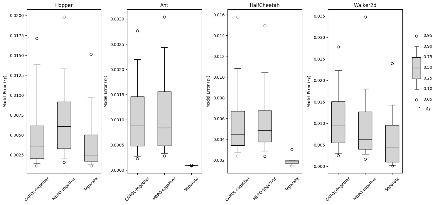
Figure 5: Demonstration of the model error distribution. CAROL-together, MBPO-together, and separate represent the distribution from the models trained with CAROL, models trained with MBPO, and the models trained from datasets from rollout with random policies, respectively.

C.3 Certified Performance When Assuming the Model Being Perfect

We demonstrate the certified performance when assuming the $\varepsilon_{E}$ being zero in Figure 6 and Figure 7. The general trend of the certified performance does not change much, while the exact Wcar $/T$ increases. Specifically, Walker2d could give reasonable certification over longer horizons.

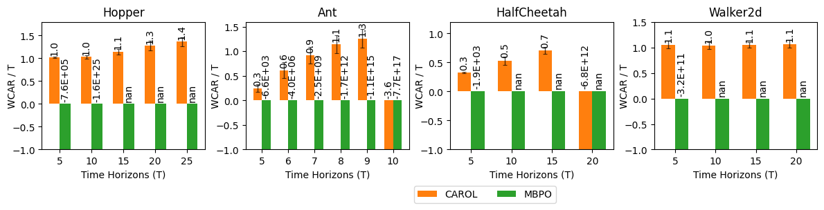
Figure 6: Certified performance of policies $\pi$ with the learned-together model, $E$. Each bar is an average of 25 starting states. The results are based on the assumption of $\varepsilon_{E}$ being $0.0$.

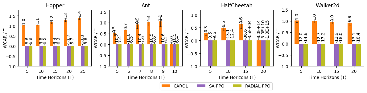
Figure 7: Certified performance of policies $\pi$ under a set of separately learned models, $\{E_{i}\}$. Each bar averages the learned policies on each $E_{i}$ of 25 starting states. The results are based on the assumption of $\varepsilon_{E}$ being $0.0$.

C.4 Certified Performance When Evaluating against Training Perturbation Range

We show the provability results with $\epsilon_{\text{test}}$ being $\epsilon_{\text{train}}$ in Figure 8 and Figure 9.

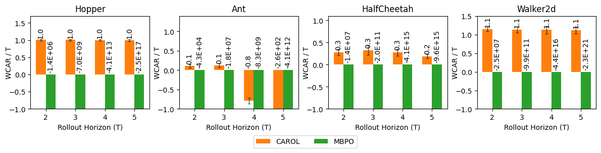
Figure 8: Certified performance of policies $\pi$ with the learned-together model, $E$. The results are based on $\varepsilon_{E}$ with a $1-\delta_{E}$ of $0.9$.

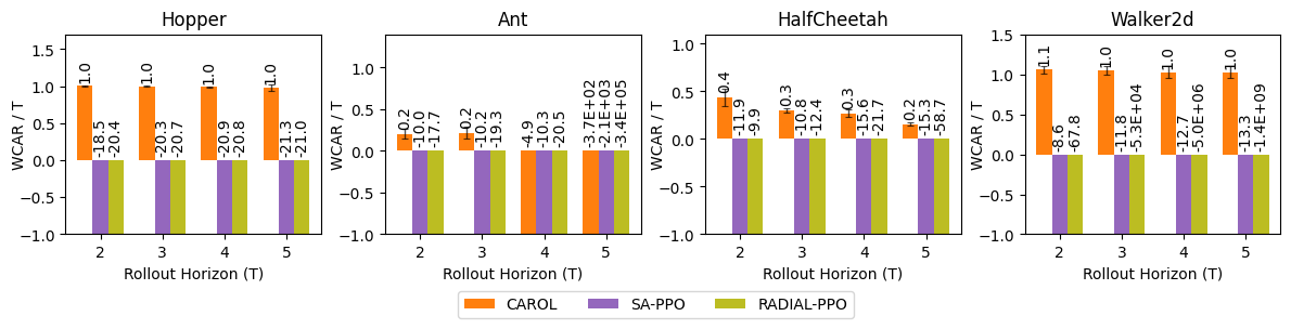
Figure 9: Certified performance of policies $\pi$ under a set of separately learned models, $\{E_{i}\}$. The results are based on $\varepsilon_{E}$ with a $1-\delta_{E}$ of $0.9$.

Appendix D Qualitative Evaluation of the Abstract Trace Lower Bound

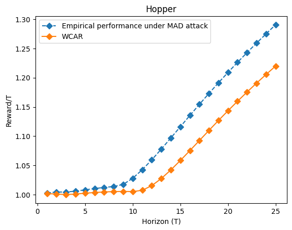
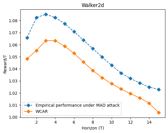
Figure 10: Examples of robustness certification of CAROL. We show the reward under one empirical attack (MAD) and WCAR (incorporating the model error with $1-\delta_{E}$ being $0.90$) over horizons starting from the same initial state.

We give our attempt to evaluate and demonstrate the lower bound of the abstract traces over CAROL with examples in Figure 10. Specifically, we show the reward under one empirical attack (MAD) and our Wcar (incorporating the model error) over horizons starting from the same initial state. Wcar being always smaller than the reward under empirical attack indicates soundness. The reasonably small gap between the two lines indicates tightness. One interesting observation is that as the horizon increases, the gap increases. We give two possible explanations for this:

• The empirical attack is not strong enough to reveal the agents’ performance under the worst-case attack.

• The overapproximation error and the model error from CAROL accumulate as the horizon increases.

Appendix E Abstract Bound Propagation

Now, we give an explanation of how interval bound propagation (IBP) works. CROWN [41] optimizes over IBP for tighter bound (specifically for Relu and sigmoid, etc.). IBP considers the box domain in the implementation. For a program with $m$ variables, each component in the domain represents a $m$-dimensional box. Each component of the domain is a pair $b=\langle b_{c},b_{e}\rangle$, where $b_{c}\in\mathbb{R}^{m}$ is the center of the box and $b_{e}\in\mathbb{R}^{m}_{\geq 0}$ represents the non-negative deviations. The interval concretization of the $i$-th dimension variable of $b$ is given by

$$[{(b_{c})}_{i}-{(b_{e})}_{i},{(b_{c})}_{i}+{(b_{e})}_{i}].$$

Now we give the abstract update for the box domain following [23].

Add.

For a concrete function $f$ that replaces the $i$-th element in the input vector $x\in\mathbb{R}^{m}$ by the sum of the $j$-th and $k$-th element:

$$f(x)=(x_{1},\dots,x_{i-1},x_{j}+x_{k},x_{i+1},\dots x_{m})^{T}.$$

The abstraction function of $f$ is given by:

$$f^{\#}(b)=\langle M\cdot b_{c},M\cdot b_{e}\rangle,$$

where $M\in\mathbb{R}^{m\times m}$ can replace the $i$-th element of $x$ by the sum of the $j$-th and $k$-th element by $M\cdot b_{c}$.

Multiplication.

For a concrete function $f$ that multiplies the $i$-th element in the input vector $x\in\mathbb{R}^{m}$ by a constant $w$:

$$f(x)=(x_{1},\dots,x_{i-1},w\cdot x_{i},x_{i+1},\dots,x_{m})^{T}.$$

The abstraction function of $f$ is given by:

$$f^{\#}(b)=\langle M_{w}\cdot b_{c},M_{|w|}\cdot b_{e}\rangle,$$

where $M_{w}\cdot b_{c}$ multiplies the $i$-th element of $b_{c}$ by $w$ and $M_{|w|}\cdot b_{e}$ multiplies the $i$-th element of $b_{e}$ with $|w|$.

Matrix Multiplication.

For a concrete function $f$ that multiplies the input $x\in\mathbb{R}^{m}$ by a fixed matrix $M\in\mathbb{R}^{m^{\prime}\times m}$:

$$f(x)=M\cdot x.$$

The abstraction function of $f$ is given by:

$$f^{\#}(b)=\langle M\cdot b_{c},|M|\cdot b_{e}\rangle,$$

where $M$ is an element-wise absolute value operation. Convolutions follow the same approach, as they are also linear operations.

ReLU.

For a concrete element-wise ReLU operation over $x\in\mathbb{R}^{m}$:

$$\textrm{ReLU}(x)=(\text{max}(x_{1},0),\dots,\text{max}(x_{m},0))^{T},$$

the abstraction function of ReLU is given by:

$$\textrm{ReLU}^{\#}(b)=\langle\frac{\textrm{ReLU}(b_{c}+b_{e})+\textrm{ReLU}(b_{c}-b_{e})}{2},\frac{\textrm{ReLU}(b_{c}+b_{e})-\textrm{ReLU}(b_{c}-b_{e})}{2}\rangle.$$

where $b_{c}+b_{e}$ and $b_{c}-b_{e}$ denotes the element-wise sum and element-wise subtraction between $b_{c}$ and $b_{e}$.

Sigmoid.

As Sigmoid and ReLU are both monotonic functions, the abstraction functions follow the same approach. For a concrete element-wise Sigmoid operation over $x\in\mathbb{R}^{m}$:

$$\textrm{Sigmoid}(x)=(\frac{1}{1+\text{exp}(-x_{1})},\dots,\frac{1}{1+\text{exp}(-x_{m})})^{T},$$

the abstraction function of Sigmoid is given by:

$$\textrm{Sigmoid}^{\#}(b)=\langle\frac{\textrm{Sigmoid}(b_{c}+b_{e})+\textrm{Sigmoid}(b_{c}-b_{e})}{2},\frac{\textrm{Sigmoid}(b_{c}+b_{e})-\textrm{Sigmoid}(b_{c}-b_{e})}{2}\rangle.$$

where $b_{c}+b_{e}$ and $b_{c}-b_{e}$ denotes the element-wise sum and element-wise subtraction between $b_{c}$ and $b_{e}$. All the above abstract updates can be easily differentiable and parallelized on the GPU.

Appendix F Broader Discussion about Limitations and Future Works

We present a detailed discussion about limitations and future directions of our work below.

Adversarial Setting.

We focus on the state-adversarial setting. There are broader adversarial settings related to model disturbances and model uncertainty [22]. Exploring the certified learning over environment dynamics perturbation is of interest. Specifically, we do not require a predefined model. We learn a model where the model misspecification amounts to supervised learning error. Future works would incorporate the potential disturbance of the environment in training to learn the dynamics model under Carol framework.

Dimensionality.

We focus on control benchmarks in this work. Related works about certification [38] use higher dimensional environments (e.g., Atari). However, the methods in CROP [38] primarily work on discrete state/action space and assume a deterministic environment. Carol is more general; while CROP does post-hoc verification, we focus on certified learning, where verification is integrated with learning. In addition, to the best of our knowledge, the environments we evaluate over have the largest dimensionality in certified RL papers [11, 3].

Stochasticity.

We have challenges in handling highly random environments, which is a fundamental limitation of all certified learning techniques. We consider the stochasticity in the theoretical analysis by incorporating the variance of $R^{\#}$in the soundness bound. When stochasticity is large, the tightness of our bound may be affected.

Complexity.

Certified learning is more expensive than regular learning due to the requirement of certifiability and soundness guarantee. In training, the symbolic state is represented by the center and the width of a box (2x information representation per state). Propagating over a box needs an additional 2x computation compared to computation without symbolic states. Consequently, Carol is approximately two times slower than the base RL algorithm per step.

In summary, Carol ’s performance is limited in the very large-scale MDPs over long rollout horizons mainly due to two reasons:

• Efficient abstract interpretation domains (e.g., Interval/Box) can give accumulated over-approximation error.

• Tighter abstract interpretation domains are expensive in training and may not be differentiable. (e.g. bounded Zonotopes [32] or Polyhedra [33]).

We believe that future works on tighter, more efficient, and differentiable abstract interpretation techniques would benefit Carol as our framework is not built on top of one particular abstract interpretation method. Additionally, a broader setting of adversarial perturbations would be an interesting future direction to extend our work.

References

- Altman [1999] Eitan Altman. Constrained Markov decision processes: stochastic modeling. Routledge, 1999.
- Brockman et al. [2016] Greg Brockman, Vicki Cheung, Ludwig Pettersson, Jonas Schneider, John Schulman, Jie Tang, and Wojciech Zaremba. Openai gym, 2016.
- Chang and Gao [2021] Ya-Chien Chang and Sicun Gao. Stabilizing neural control using self-learned almost lyapunov critics. In 2021 IEEE International Conference on Robotics and Automation (ICRA), pages 1803–1809. IEEE, 2021.
- Cheng et al. [2019a] Richard Cheng, Gábor Orosz, Richard M Murray, and Joel W Burdick. End-to-end safe reinforcement learning through barrier functions for safety-critical continuous control tasks. In Proceedings of the AAAI Conference on Artificial Intelligence, volume 33, pages 3387–3395, 2019a.
- Cheng et al. [2019b] Richard Cheng, Abhinav Verma, Gabor Orosz, Swarat Chaudhuri, Yisong Yue, and Joel Burdick. Control regularization for reduced variance reinforcement learning. In International Conference on Machine Learning, pages 1141–1150. PMLR, 2019b.
- Chow et al. [2018] Yinlam Chow, Ofir Nachum, Edgar Duenez-Guzman, and Mohammad Ghavamzadeh. A lyapunov-based approach to safe reinforcement learning. Advances in neural information processing systems, 31, 2018.
- Chow et al. [2019] Yinlam Chow, Ofir Nachum, Aleksandra Faust, Edgar Duenez-Guzman, and Mohammad Ghavamzadeh. Lyapunov-based safe policy optimization for continuous control. arXiv preprint arXiv:1901.10031, 2019.
- Cohen et al. [2019] Jeremy Cohen, Elan Rosenfeld, and Zico Kolter. Certified adversarial robustness via randomized smoothing. In International Conference on Machine Learning, pages 1310–1320. PMLR, 2019.
- Cousot and Cousot [1977] P. Cousot and R. Cousot. Abstract interpretation: a unified lattice model for static analysis of programs by construction or approximation of fixpoints. In Conference Record of the Fourth Annual ACM SIGPLAN-SIGACT Symposium on Principles of Programming Languages, pages 238–252, Los Angeles, California, 1977. ACM Press, New York, NY.
- Dawson et al. [2022a] Charles Dawson, Sicun Gao, and Chuchu Fan. Safe control with learned certificates: A survey of neural lyapunov, barrier, and contraction methods. arXiv preprint arXiv:2202.11762, 2022a.
- Dawson et al. [2022b] Charles Dawson, Zengyi Qin, Sicun Gao, and Chuchu Fan. Safe nonlinear control using robust neural lyapunov-barrier functions. In Conference on Robot Learning, pages 1724–1735. PMLR, 2022b.
- Everett et al. [2021] Michael Everett, Björn Lütjens, and Jonathan P How. Certifiable robustness to adversarial state uncertainty in deep reinforcement learning. IEEE Transactions on Neural Networks and Learning Systems, 2021.
- Fischer et al. [2019] Marc Fischer, Matthew Mirman, Steven Stalder, and Martin Vechev. Online robustness training for deep reinforcement learning. arXiv preprint arXiv:1911.00887, 2019.
- Gleave et al. [2019] Adam Gleave, Michael Dennis, Cody Wild, Neel Kant, Sergey Levine, and Stuart Russell. Adversarial policies: Attacking deep reinforcement learning. arXiv preprint arXiv:1905.10615, 2019.
- Gowal et al. [2018] Sven Gowal, Krishnamurthy Dvijotham, Robert Stanforth, Rudy Bunel, Chongli Qin, Jonathan Uesato, Relja Arandjelovic, Timothy Mann, and Pushmeet Kohli. On the effectiveness of interval bound propagation for training verifiably robust models. arXiv preprint arXiv:1810.12715, 2018.
- Huang et al. [2017] Sandy Huang, Nicolas Papernot, Ian Goodfellow, Yan Duan, and Pieter Abbeel. Adversarial attacks on neural network policies. arXiv preprint arXiv:1702.02284, 2017.
- Janner et al. [2019] Michael Janner, Justin Fu, Marvin Zhang, and Sergey Levine. When to trust your model: Model-based policy optimization. Advances in Neural Information Processing Systems, 32, 2019.
- Kumar et al. [2021] Aounon Kumar, Alexander Levine, and Soheil Feizi. Policy smoothing for provably robust reinforcement learning. In International Conference on Learning Representations, 2021.
- Li and Belta [2019] Xiao Li and Calin Belta. Temporal logic guided safe reinforcement learning using control barrier functions. arXiv preprint arXiv:1903.09885, 2019.
- Lin et al. [2017] Yen-Chen Lin, Zhang-Wei Hong, Yuan-Hong Liao, Meng-Li Shih, Ming-Yu Liu, and Min Sun. Tactics of adversarial attack on deep reinforcement learning agents. arXiv preprint arXiv:1703.06748, 2017.
- Lütjens et al. [2020] Björn Lütjens, Michael Everett, and Jonathan P How. Certified adversarial robustness for deep reinforcement learning. In Conference on Robot Learning, pages 1328–1337. PMLR, 2020.
- Mankowitz et al. [2019] Daniel J Mankowitz, Nir Levine, Rae Jeong, Yuanyuan Shi, Jackie Kay, Abbas Abdolmaleki, Jost Tobias Springenberg, Timothy Mann, Todd Hester, and Martin Riedmiller. Robust reinforcement learning for continuous control with model misspecification. arXiv preprint arXiv:1906.07516, 2019.
- Mirman et al. [2018] Matthew Mirman, Timon Gehr, and Martin Vechev. Differentiable abstract interpretation for provably robust neural networks. In International Conference on Machine Learning, pages 3578–3586. PMLR, 2018.
- Mnih et al. [2015] Volodymyr Mnih, Koray Kavukcuoglu, David Silver, Andrei A Rusu, Joel Veness, Marc G Bellemare, Alex Graves, Martin Riedmiller, Andreas K Fidjeland, Georg Ostrovski, et al. Human-level control through deep reinforcement learning. nature, 518(7540):529–533, 2015.
- Nandwani et al. [2019] Yatin Nandwani, Abhishek Pathak, Mausam, and Parag Singla. A primal dual formulation for deep learning with constraints. In H. Wallach, H. Larochelle, A. Beygelzimer, F. d'Alché-Buc, E. Fox, and R. Garnett, editors, Advances in Neural Information Processing Systems, volume 32. Curran Associates, Inc., 2019. URL https://proceedings.neurips.cc/paper/2019/file/cf708fc1decf0337aded484f8f4519ae-Paper.pdf.
- Oikarinen et al. [2021] Tuomas Oikarinen, Wang Zhang, Alexandre Megretski, Luca Daniel, and Tsui-Wei Weng. Robust deep reinforcement learning through adversarial loss. Advances in Neural Information Processing Systems, 34:26156–26167, 2021.
- Pineda et al. [2021] Luis Pineda, Brandon Amos, Amy Zhang, Nathan O. Lambert, and Roberto Calandra. Mbrl-lib: A modular library for model-based reinforcement learning. Arxiv, 2021. URL https://arxiv.org/abs/2104.10159.
- Pinto et al. [2017] Lerrel Pinto, James Davidson, Rahul Sukthankar, and Abhinav Gupta. Robust adversarial reinforcement learning. In International Conference on Machine Learning, pages 2817–2826. PMLR, 2017.
- Polydoros and Nalpantidis [2017] Athanasios S Polydoros and Lazaros Nalpantidis. Survey of model-based reinforcement learning: Applications on robotics. Journal of Intelligent & Robotic Systems, 86(2):153–173, 2017.
- Russo and Proutiere [2019] Alessio Russo and Alexandre Proutiere. Optimal attacks on reinforcement learning policies. arXiv preprint arXiv:1907.13548, 2019.
- Sallab et al. [2017] Ahmad EL Sallab, Mohammed Abdou, Etienne Perot, and Senthil Yogamani. Deep reinforcement learning framework for autonomous driving. Electronic Imaging, 2017(19):70–76, 2017.
- Scott et al. [2016] Joseph K Scott, Davide M Raimondo, Giuseppe Roberto Marseglia, and Richard D Braatz. Constrained zonotopes: A new tool for set-based estimation and fault detection. Automatica, 69:126–136, 2016.
- Singh et al. [2017] Gagandeep Singh, Markus Püschel, and Martin Vechev. Fast polyhedra abstract domain. In Proceedings of the 44th ACM SIGPLAN Symposium on Principles of Programming Languages, pages 46–59, 2017.
- Sun et al. [2021] Yanchao Sun, Ruijie Zheng, Yongyuan Liang, and Furong Huang. Who is the strongest enemy? towards optimal and efficient evasion attacks in deep rl. arXiv preprint arXiv:2106.05087, 2021.
- Sutton [1990] Richard S. Sutton. Integrated architecture for learning, planning, and reacting based on approximating dynamic programming. In Proceedings of the Seventh International Conference (1990) on Machine Learning, page 216–224, San Francisco, CA, USA, 1990. Morgan Kaufmann Publishers Inc. ISBN 1558601414.
- Weng et al. [2019] Tsui-Wei Weng, Krishnamurthy Dj Dvijotham, Jonathan Uesato, Kai Xiao, Sven Gowal, Robert Stanforth, and Pushmeet Kohli. Toward evaluating robustness of deep reinforcement learning with continuous control. In International Conference on Learning Representations, 2019.
- Wong and Kolter [2018] Eric Wong and Zico Kolter. Provable defenses against adversarial examples via the convex outer adversarial polytope. In International Conference on Machine Learning, pages 5286–5295. PMLR, 2018.
- Wu et al. [2021] Fan Wu, Linyi Li, Zijian Huang, Yevgeniy Vorobeychik, Ding Zhao, and Bo Li. Crop: Certifying robust policies for reinforcement learning through functional smoothing. In International Conference on Learning Representations, 2021.
- Xu et al. [2020] Kaidi Xu, Zhouxing Shi, Huan Zhang, Minlie Huang, K Chang, Bhavya Kailkhura, Xue Lin, and C Hsieh. Automatic perturbation analysis on general computational graphs. Technical report, Lawrence Livermore National Lab.(LLNL), Livermore, CA (United States), 2020.
- Yang and Chaudhuri [2021] Chenxi Yang and Swarat Chaudhuri. Safe neurosymbolic learning with differentiable symbolic execution. In International Conference on Learning Representations, 2021.
- Zhang et al. [2018] Huan Zhang, Tsui-Wei Weng, Pin-Yu Chen, Cho-Jui Hsieh, and Luca Daniel. Efficient neural network robustness certification with general activation functions. Advances in neural information processing systems, 31, 2018.
- Zhang et al. [2020] Huan Zhang, Hongge Chen, Chaowei Xiao, Bo Li, Mingyan Liu, Duane Boning, and Cho-Jui Hsieh. Robust deep reinforcement learning against adversarial perturbations on state observations. Advances in Neural Information Processing Systems, 33:21024–21037, 2020.
- Zhang et al. [2021] Huan Zhang, Hongge Chen, Duane Boning, and Cho-Jui Hsieh. Robust reinforcement learning on state observations with learned optimal adversary. arXiv preprint arXiv:2101.08452, 2021.