A Robust Optimisation Perspective on
Counterexample-Guided Repair of Neural Networks

Abstract

Counterexample-guided repair aims at creating neural networks with mathematical safety guarantees, facilitating the application of neural networks in safety-critical domains. However, whether counterexample-guided repair is guaranteed to terminate remains an open question. We approach this question by showing that counterexample-guided repair can be viewed as a robust optimisation algorithm. While termination guarantees for neural network repair itself remain beyond our reach, we prove termination for more restrained machine learning models and disprove termination in a general setting. We empirically study the practical implications of our theoretical results, demonstrating the suitability of common verifiers and falsifiers for repair despite a disadvantageous theoretical result. Additionally, we use our theoretical insights to devise a novel algorithm for repairing linear regression models based on quadratic programming, surpassing existing approaches.

proofidea

Proof Idea.

Oθnet_#1

1 Introduction

The success of artificial neural networks in such diverse domains as image recognition (LeCun et al., 1998), natural language processing (Brown et al., 2020), predicting protein folding (Senior et al., 2020), and designing novel algorithms (Fawzi et al., 2022) sparks interest in applying them to more demanding tasks, including applications in safety-critical domains. Neural networks are proposed to be used for medical diagnosis (Amato et al., 2013), autonomous aircraft control (Jorgensen, 1997; Julian et al., 2018), and self-driving cars (Bojarski et al., 2016). Since a malfunctioning of such systems can threaten lives or cause environmental disaster, we require mathematical guarantees on the correct functioning of the neural networks involved. Formal methods, including verification and repair, allow obtaining such guarantees (Pulina & Tacchella, 2010). As the inner workings of neural networks are opaque to human engineers, automated repair is a vital component for creating safe neural networks.

Alternating search for violations and removal of violations is a popular approach for repairing neural networks (Pulina & Tacchella, 2010; Goodfellow et al., 2015; Guidotti et al., 2019a; Dong et al., 2021; Goldberger et al., 2020; Sivaraman et al., 2020; Tan et al., 2021; Bauer-Marquart et al., 2022). We study this approach under the name counterexample-guided repair. Counterexample-guided repair uses inputs for which a neural network violates the specification (counterexamples) to iteratively refine the network until the network satisfies the specification. While empirical results demonstrate the ability of counterexample-guided repair to successfully repair neural networks (Bauer-Marquart et al., 2022), a theoretical analysis of counterexample-guided repair is lacking.

In this paper, we study counterexample-guided repair from the perspective of robust optimisation. Viewing counterexample-guided repair as an algorithm for solving robust optimisation problems allows us to encircle neural network repair from two sides. On the one hand side, we are able to show termination and optimality for counterexample-guided repair of linear regression models and linear classifiers, as well as single ReLU neurons. Coming from the other side, we disprove termination for repairing ReLU networks to satisfy a specification with an unbounded input set. Additionally, we disprove termination of counterexample-guided repair when using generic counterexamples without further qualifications, such as being most-violating. While we could not address termination for the precise robust program of neural network repair with specifications having bounded input sets, such as $L_{\infty}$ adversarial robustness or the ACAS Xu safety properties (Katz et al., 2017), our robust optimisation framework provides, for the first time to the best of our knowledge, fundamental insights into the theoretical properties of counterexample-guided repair.

Our analysis establishes a theoretical limitation of repair with otherwise unqualified counterexamples and suggests most-violating counterexamples as a replacement. We empirically investigate the practical consequences of these findings by comparing early-exit verifiers — verifiers that stop search on the first counterexample they encounter — and optimal verifiers that produce most-violating counterexamples. We complement this experiment by investigating the advantages of using falsifiers during repair (Bauer-Marquart et al., 2022), which is another approach that leverages sub-optimal counterexamples. These experiments do not reveal any practical limitations for repair using early-exit verifiers. In fact, using an early-exit verifier consistently yields faster repair for ACAS Xu networks (Katz et al., 2017) and an MNIST (LeCun et al., 1998) network, compared to using an optimal verifier. While the optimal verifier often allows performing fewer iterations, this advantage is offset by its additional runtime cost most of the time. Our experiments with falsifiers demonstrate that they can provide a significant runtime advantage for neural network repair.

For repairing linear regression models, we use our theoretical insights to design an improved repair algorithm based on quadratic programming. We compare this new algorithm with the Ouroboros (Tan et al., 2021) and SpecRepair (Bauer-Marquart et al., 2022) repair algorithms. The new quadratic programming repair algorithm surpasses Ouroboros and SpecRepair, illustrating the practical relevance of our theoretical results.

We highlight the following main contributions of this paper:

1. We formalise neural network repair as a robust optimisation problem and, therefore, view counterexample-guided repair as a robust optimisation algorithm.

2. Using this theoretical framework, we prove termination of counterexample-guided repair for more restrained problems than neural network repair and disprove termination in a more general setting.

3. We empirically investigate the merits of using falsifiers and early-exit verifiers during repair.

4. Our theoretical insights into repairing linear regression models allow us to surpass existing approaches for repairing linear regression models using a new repair algorithm.

2 Related Work

This paper is concerned with viewing neural network repair through the lens of robust optimisation. Neural network repair relies on neural network verification and can make use of neural network falsification. Counterexample-guided repair is related to other counterexample-guided algorithms. We introduce related work from these fields in this section.

Neural Network Verification We can verify neural networks, for example, using Satisfiability Modulo Theories (SMT) solving (Katz et al., 2017; Ehlers, 2017) or Mixed Integer Linear Programming (MILP) (Tjeng et al., 2019). Verification benefits from bounds computed using linear relaxations (Ehlers, 2017; Singh et al., 2018; Zhang et al., 2018; Xu et al., 2021). A particularly fruitful technique from MILP is branch and bound (Bunel et al., 2018; Palma et al., 2021; Wang et al., 2021). Approaches that combine branch and bound with multi-neuron linear relaxations (Ferrari et al., 2022) or extend branch and bound using cutting planes (Zhang et al., 2022b) form the current state-of-the-art (Müller et al., 2022).

Falsifiers are designed to discover counterexamples fast at the cost of completeness — they can not prove specification satisfaction. We view adversarial attacks as falsifiers for adversarial robustness specifications. Falsifiers use generic local optimisation algorithms (Szegedy et al., 2014; Goodfellow et al., 2015; Kurakin et al., 2017; Madry et al., 2018), global optimisation algorithms (Uesato et al., 2018; Bauer-Marquart et al., 2022), or specifically tailored search and optimisation techniques (Papernot et al., 2015; Chen et al., 2020).

Neural Network Repair Neural network repair is concerned with modifying a neural network such that it satisfies a formal specification. Many approaches make use of the counterexample-guided repair algorithm while utilising different counterexample-removal algorithms. The approaches range from augmenting the training set (Pulina & Tacchella, 2010; Goodfellow et al., 2015; Tan et al., 2021), over specialised neural network architectures (Guidotti et al., 2019a; Dong et al., 2021), and neural network training with constraints (Bauer-Marquart et al., 2022), to using a verifier for computing network weights (Goldberger et al., 2020). Counterexample-guided repair is also applied to support vector machines (SVMs) and linear regression models (Guidotti et al., 2019b; Tan et al., 2021). Using decoupled neural networks (Sotoudeh & Thakur, 2021) provides optimality and termination guarantees for repair but is limited to two-dimensional input spaces.

When considering only adversarial robustness, an alternative to counterexample-guided repair is provably robust training. Here, the applied techniques include interval arithmetic (Gowal et al., 2018), semi-definite relaxations (Raghunathan et al., 2018), linear relaxations (Mirman et al., 2018), and duality (Wong & Kolter, 2018). Also specialised neural network architectures can increase the adversarial robustness of neural networks (Cissé et al., 2017; Zhang et al., 2022a).

Robust and Scenario Optimisation Robust optimisation is, originally, a technique for dealing with data uncertainty (Ben-Tal et al., 2009). Although robust optimisation problems are, in general, NP-hard (Ben-Tal & Nemirovski, 1998), polynomial-time methods exist in many —typically convex — settings (Ben-Tal et al., 2009). Scenario problems and chance-constrained problems relax robust problems. Feasibility for a scenario problem can be linked to feasibility for a chance-constrained problem (Campi & Garatti, 2008) and even to a perturbed robust problem (Esfahani et al., 2015). In this paper, we consider the worst-case perspective on robust optimisation (Mutapcic & Boyd, 2009).

Loss functions based on robust optimisation can be used to train for adversarial robustness and beyond (Madry et al., 2018; Wong & Kolter, 2018; Fischer et al., 2019). We study a different robust optimisation formulation, where the specification is modelled as constraints.

Counterexample-Guided Algorithms Besides neural network repair, counterexample-guided approaches are also used in model checking (Clarke et al., 2000), program synthesis (Solar-Lezama et al., 2006), and beyond (Henzinger et al., 2003; Reynolds et al., 2015; Nguyen et al., 2017). The notion of minimal counterexamples in program synthesis (Jha & Seshia, 2014), which is based on an ordering of the counterexamples, encompasses our notion of most-violating counterexamples. While related, the termination results for counterexample-guided program synthesis (Solar-Lezama et al., 2006) do not transfer to repairing neural networks, as they only apply for finite input domains. We study infinite input domains in this paper.

3 Preliminaries and Problem Statement

In this section, we introduce preliminaries on robust optimisation, neural networks, and neural network verification before progressing to neural network repair, counterexample-guided repair, and the problem statement of our theoretical analysis.

3.1 Robust Optimisation

We consider general robust optimisation problems of the form

$$P:\left\{\!\begin{array}[]{cl}\underset{\mathbf{v}}{\text{minimise}}&f(\mathbf{v})\\ \text{subject to}&g{\left(\mathbf{v},\mathbf{d}\right)}\geq 0\quad\forall\mathbf{d}\in\mathcal{D}\\ &\mathbf{v}\in\mathcal{V},\end{array}\right.$$ (1)

where $\mathcal{V}\subseteq\mathbb{R}^{v}$, $\mathcal{D}\subseteq\mathbb{R}^{d}$ and $f:\mathcal{V}\to\mathbb{R}$, $g:\mathcal{V}\times\mathcal{D}\to\mathbb{R}$. Both $\mathcal{V}$ and $\mathcal{D}$ contain infinitely many elements. Therefore, a robust optimisation problem has infinitely many constraints. The variable domain $\mathcal{V}$ defines eligible values for the optimisation variable $\mathbf{v}$. The set $\mathcal{D}$ may contain, for example, all inputs for which a specification needs to hold. In this example, $g$ captures whether the specification is satisfied for a concrete input. Elaborating this example leads to neural network repair, which we introduce in Section 3.4.

A scenario optimisation problem relaxes a robust optimisation problem by replacing the infinitely many constraints of $P$ with a finite selection. For $\mathbf{d}^{(i)}\in\mathcal{D}$, $i\in\{1,\ldots,N\}$, $N\in\mathbb{N}$, the scenario optimisation problem is

$${S\!\!\>P}:\left\{\!\begin{array}[]{cl}\underset{\mathbf{v}}{\text{minimise}}&f(\mathbf{v})\\ \text{subject to}&g{\left(\mathbf{v},\mathbf{d}^{(i)}\right)}\geq 0\quad\forall i\in\{1,\ldots,N\}\\ &\mathbf{v}\in\mathcal{V}.\end{array}\right.$$ (2)

The counterexample-guided repair algorithm that we study in this paper uses a sequence of scenario optimisation problems to solve a robust optimisation problem.

3.2 Neural Networks

A neural network $\NN{}:\mathbb{R}^{n}\to\mathbb{R}^{m}$, with parameters $\bm{\theta}\in\mathbb{R}^{p}$ is a function composition of affine transformations and non-linear activations. For our theoretical analysis, it suffices to consider fully-connected neural networks (FCNN). Our experiments in Section 5 also use convolutional neural networks (CNN). We refer to Goodfellow et al. (2016) for an introduction to CNNs. An FCNN with $L$ hidden layers is a chain of affine functions and activation functions

$$\NN{}=h^{(L+1)}\circ\sigma^{(L)}\circ h^{(L)}\circ\cdots\circ\sigma^{(1)}\circ h^{(1)},$$ (3)

where $h^{(i)}:\mathbb{R}^{n_{i-1}}\to\mathbb{R}^{n_{i}}$ and $\sigma^{(i)}:\mathbb{R}^{n_{i}}\to\mathbb{R}^{n_{i}}$ with $n_{i}\in\mathbb{N}$ for $i\in\{0,\ldots,L+1\}$ and, specifically, $n_{0}=n$ and $n_{L+1}=m$. Each $h^{(i)}$ is an affine function, called an affine layer. It computes $h^{(i)}(\mathbf{z})=\mathbf{W}^{(i)}\mathbf{z}+\mathbf{b}^{(i)}$ with weight matrix $\mathbf{W}^{(i)}\in\mathbb{R}^{n_{i}\times n_{i-1}}$ and bias vector $\mathbf{b}^{(i)}\in\mathbb{R}^{n_{i}}$. Stacked into one large vector, the weights and biases of all affine layers are the parameters $\bm{\theta}$ of the FCNN. An activation layer $\sigma^{(i)}$ applies a non-linear function, such as ReLU ${\left[z\right]}^{+}=\max(0,z)$ or the sigmoid function $\sigma(z)=\frac{1}{1+e^{-z}}$ in an element-wise fashion.

3.3 Neural Network Verification

Neural network verification is concerned with automatically proving that a neural network satisfies a formal specification.

Definition 3.1 (Specification).

A specification $\Phi=\{\varphi_{1},\ldots,\varphi_{S}\}$ is a set of properties $\varphi_{i}$. A property $\varphi=(\mathcal{X}_{\varphi},\mathcal{Y}_{\varphi})$ is a tuple of an input set $\mathcal{X}_{\varphi}\subseteq\mathbb{R}^{n}$ and an output set $\mathcal{Y}_{\varphi}\subseteq\mathbb{R}^{m}$.

We write $\NN\vDash\Phi$ when a neural network $\NN:\mathbb{R}^{n}\to\mathbb{R}^{m}$ satisfies a specification $\Phi$. Specifically,

$$\NN\vDash\Phi \Leftrightarrow\forall\varphi\in\Phi:\NN\vDash\varphi$$ (4a)

$$\NN\vDash\varphi \Leftrightarrow\forall\mathbf{x}\in\mathcal{X}_{\varphi}:\NN(\mathbf{x})\in\mathcal{Y}_{\varphi}.$$ (4b)

Example specifications, such as $L_{\infty}$ adversarial robustness or an ACAS Xu safety specification (Katz et al., 2017) are defined in Appendix C.

Counterexamples are at the core of the counterexample-guided repair algorithm that we study in this paper.

Definition 3.2 (Counterexample).

An input $\mathbf{x}\in\mathcal{X}_{\varphi}$ for which a neural network $\NN$ violates a property $\varphi$ is called a counterexample.

To define verification as an optimisation problem, we introduce satisfaction functions. A satisfaction function quantifies the satisfaction or violation of a property regarding the output set. Definition 3.4 introduces the verification problem, also taking the input set of a property into account.

Definition 3.3 (Satisfaction Function).

A function $f_{\mathrm{Sat}}{}:\mathbb{R}^{m}\to\mathbb{R}$ is a satisfaction function of a property $\varphi=(\mathcal{X}_{\varphi},\mathcal{Y}_{\varphi})$ if $\mathbf{y}\in\mathcal{Y}_{\varphi}\Leftrightarrow f_{\mathrm{Sat}}(\mathbf{y})\geq 0$.

Definition 3.4 (Verification Problem).

The verification problem for a property $\varphi=(\mathcal{X}_{\varphi},\mathcal{Y}_{\varphi})$ and a neural network $\NN$ is

$$V:f_{\mathrm{Sat}}^{\ast}=\left\{\!\begin{array}[]{cl}\underset{\mathbf{x}}{\text{minimise}}&f_{\mathrm{Sat}}(\NN(\mathbf{x}))\\ \text{subject to}&\mathbf{x}\in\mathcal{X_{\varphi}}.\end{array}\right.$$ (5)

We call a specification a linear specification when its properties have a closed convex polytope as an input set and an affine satisfaction function. Appendix C contains several examples of satisfaction functions from SpecRepair (Bauer-Marquart et al., 2022). The following Proposition follows directly from the definition of a satisfaction function.

Proposition 3.5.

A neural network $\NN$ satisfies the property $\varphi$ if and only if the minimum of the verification problem $V$ ($f_{\mathrm{Sat}}^{\ast}$) is non-negative.

We now consider counterexample searchers that evaluate the satisfaction function for concrete inputs to compute an upper bound on the minimum of the verification problem $V$. Such tools can disprove specification satisfaction by discovering a counterexample. They can also prove specification satisfaction when they are sound and complete.

Definition 3.6 (Soundness and Completeness).

We call a counterexample searcher sound if it computes valid upper bounds and complete if it is guaranteed to find a counterexample whenever a counterexample exists.

Definition 3.7 (Verifiers and Falsifiers).

We call a sound and complete counterexample searcher a verifier. A sound but incomplete counterexample searcher is a falsifier.

Definition 3.8 (Optimal and Early-Exit Verifiers).

An optimal verifier is a verifier that always produces a global minimiser of the verification problem — a most-violating counterexample. An early-exit verifier aborts on the first counterexample it encounters. It provides any counterexample, without further qualifications.

We can perform verification through global minimisation of the verification problem from Equation (5). For ReLU-activated neural networks, global minimisation is possible, for example, using Mixed Integer Linear Programming (MILP) (Cheng et al., 2017; Lomuscio & Maganti, 2017). Falsifiers may perform local optimisation using projected gradient descent (PGD) (Kurakin et al., 2017; Madry et al., 2018) to become sound but not complete. We name the approach of using PGD for falsification BIM, abbreviating the name Basic Iterative Method used by Kurakin et al. (2017).

3.4 Neural Network Repair

Neural network repair means modifying a trained neural network so that it satisfies a specification it would otherwise violate. While the primary goal of repair is satisfying the specification, the key secondary goal is that the repaired neural network still performs well on the intended task. This secondary goal can be captured using a performance measure, such as the training loss function (Bauer-Marquart et al., 2022) or the distance between the modified and the original network parameters (Goldberger et al., 2020).

Definition 3.9 (Repair Problem).

Given a neural network $\NN$, a property $\varphi=(\mathcal{X}_{\varphi},\mathcal{Y}_{\varphi})$ and a performance measure $J:\mathbb{R}^{p}\to\mathbb{R}$, repair translates to solving the repair problem

$$R:\left\{\!\begin{array}[]{cl}\underset{\bm{\theta}\in\mathbb{R}^{p}}{\text{minimise}}&J(\bm{\theta})\\ \text{subject to}&f_{\mathrm{Sat}}(\NN(\mathbf{x}))\geq 0\quad\forall\mathbf{x}\in\mathcal{X}_{\varphi}.\end{array}\right.$$ (6)

The repair problem $R$ is an instance of a robust optimisation problem as defined in Equation (1). Checking whether a parameter $\bm{\theta}$ is feasible for $R$ corresponds to verification. In particular, we can equivalently reformulate $R$ using the verification problem’s minimum $f_{\mathrm{Sat}}^{\ast}$ from Equation (5) as

$$R^{\prime}:\left\{\!\begin{array}[]{cl}\underset{\bm{\theta}\in\mathbb{R}^{p}}{\text{minimise}}&J(\bm{\theta})\\ \text{subject to}&f_{\mathrm{Sat}}^{\ast}\geq 0.\end{array}\right.$$ (7)

We stress several characteristics of the repair problem that we relax or strengthen in Section 4. First of all, $\NN$ is a neural network and we repair all parameters $\bm{\theta}$ of the network jointly. Practically, $\NN$ is a ReLU-activated FCNN or CNN, as these are the models most verifiers support. For typical specifications, such as $L_{\infty}$ adversarial robustness or the ACAS Xu safety specifications (Katz et al., 2017), the property input set $\mathcal{X}_{\varphi}$ is a hyper-rectangle. Hyper-rectangles are closed convex polytopes and, therefore, bounded.

3.5 Counterexample-Guided Repair

In the previous section, we have seen that the repair problem includes the verification problem as a sub-problem. Using this insight, a natural approach to tackle the repair problem is to iterate running a verifier and removing the counterexamples it finds. This yields the counterexample-guided repair algorithm, that was first introduced by Goldberger et al. (2020), in a similar form. Removing counterexamples corresponds to a scenario optimisation problem ${C\!\!\>R}_{N}$ of the robust optimisation problem $R$ from Equation (6), where

$${C\!\!\>R}_{N}:\left\{\!\begin{array}[]{cl}\underset{\bm{\theta}\in\mathbb{R}^{p}}{\text{minimise}}&J(\bm{\theta})\\ \text{subject to}&f_{\mathrm{Sat}}{\left(\NN{\left(\mathbf{x}^{(i)}\right)}\right)}\geq 0\\ &\qquad\qquad\quad\forall i\in\{1,\ldots,N\}.\end{array}\right.$$ (8)

Algorithm 1 defines the counterexample-guided repair algorithm using ${C\!\!\>R}_{N}$ and $V$ from Equation (5). In analogy to ${C\!\!\>R}_{N}$, we use $V_{N}$ to denote the verification problem in iteration $N$. Concretely,

$$V_{N}:\left\{\!\begin{array}[]{cl}\underset{\mathbf{x}}{\text{minimise}}&f_{\mathrm{Sat}}(\NN[\theta^{(N-1)}](\mathbf{x}))\\ \text{subject to}&\mathbf{x}\in\mathcal{X_{\varphi}}.\end{array}\right.$$ (9)

We call the iterations of Algorithm 1 repair steps.

Algorithm 1 is concerned with repairing a single property. However, the algorithm extends to repairing multiple properties by adding one constraint for each property to ${C\!\!\>R}_{N}$ and verifying the properties separately. While Algorithm 1 is formulated for the repair problem $R$, it is easy to generalise it to any robust program $P$ as defined in Equation (1). Then, solving ${C\!\!\>R}_{N}$ corresponds to solving ${S\!\!\>P}$ from Equation (2) and solving $V_{N}$ corresponds to finding maximal constraint violations of $P$.

The question we are concerned with in this paper is whether Algorithm 1 is guaranteed to terminate after finitely many repair steps. We investigate this question in the following section by studying robust programs that are similar to the repair problem for neural networks and typical specifications, but either more restrained or more general.

Algorithm 1 Counterexample-Guided Repair

  $N\leftarrow 0$

  repeat

     // counterexample-removal (8)

     $\bm{\theta}^{(N)}\leftarrow$ local minimiser of ${C\!\!\>R}_{N}$

     $N\leftarrow N+1$ 

     // verification (9)

     $\mathbf{x}^{(N)}\leftarrow$ global minimiser of $V_{N}$

  until $f_{\mathrm{Sat}}{\left(\NN[\bm{\theta}^{(N-1)}]{\left(\mathbf{x}^{(N)}\right)}\right)}\geq 0$

4 Termination Results for Algorithm 1

The counterexample-guided repair algorithm (Algorithm 1) repairs neural networks by iteratively searching and removing counterexamples. In this section, we study whether Algorithm 1 is guaranteed to terminate and whether it produces optimally repaired networks. Our primary focus is on studying robust optimisation problems that are more restrained or more general than the repair problem $R$ from Equation (6). We apply Algorithm 1 to such problems and study termination of the algorithm for these problems. On our way, we also address the related questions of optimality on termination and termination when using an early-exit verifier as introduced in Definition 3.8.

Table 1: Symbol Overview

Symbol	Meaning
$R$	Repair Problem (6)
${C\!\!\>R}_{N}$	Counterexample Removal Problem (8)
$V_{N}$	Verification Problem for $\NN[\bm{\theta}^{(N-1)}]$ (9)
$\bm{\theta}^{\dagger}$	(Local) minimiser of $R$
$\bm{\theta}^{(N)}$	(Local) minimiser of ${C\!\!\>R}_{N}$
$\mathbf{x}^{(N)}$	Global minimiser of $V_{N}$

Table 1 summarises the central problem and variable names that we use throughout this paper. The iterations of Algorithm 1 are called repair steps. We count the repair steps starting from one but index the counterexample-removal problems starting from zero, reflecting the number of constraints. Hence, the minimiser of the counterexample-removal problem ${C\!\!\>R}_{N-1}$ from Equation (8) in repair step $N$ is $\bm{\theta}^{(N-1)}$. The verification problem in repair step $N$ is $V_{N}$ with a global minimiser $\mathbf{x}^{(N)}$.

4.1 Optimality on Termination

We prove that when applied to any robust program $P$ as defined in Equation (1), counterexample-guided repair produces a minimiser of $P$ whenever it terminates. While Algorithm 1 is formulated for the repair problem $R$, it is easy to generalise it to $P$, as described in Section 3.5. The following proposition holds regardless of whether we search for a local minimiser or a global minimiser of $R$.

Proposition 4.1 (Optimality on Termination).

Whenever Algorithm 1 terminates after $\overline{N}$ iterations, it holds that $\bm{\theta}^{(\overline{N}-1)}=\bm{\theta}^{\dagger}$.

We defer the proof of Proposition 4.1 to Appendix A.1.

4.2 Non-Termination for General Robust Programs

In this section, we demonstrate non-termination and divergence of Algorithm 1 when we relax the assumptions on the repair problem $R$ that we outline in Section 3.4. In particular, we drop the assumption that the property’s input set $\mathcal{X}_{\varphi}$ is bounded. We disprove termination by example when $\mathcal{X}_{\varphi}$ is unbounded. To simplify the proof, we use a non-standard neural network architecture. We also present a fully-connected neural network (FCNN) that similarly leads to non-termination. However, for this FCNN we also have to relax the assumption that we repair all parameters of a neural network jointly. Instead, we repair an individual parameter of the FCNN in isolation.

Proposition 4.2 (General Non-Termination).

Algorithm 1 is not guaranteed to terminate for $J:\mathbb{R}^{2}\to\mathbb{R}$, $f_{\mathrm{Sat}}:\mathbb{R}^{2}\to\mathbb{R}$, and $\NN:\mathbb{R}\to\mathbb{R}^{2}$, where $J(\bm{\theta})={\NN(0)}_{1}$, $f_{\mathrm{Sat}}(\mathbf{y})=\mathbf{y}_{2}+\mathbf{y}_{1}-1$, $\mathcal{X}_{\varphi}=\mathbb{R}$, and

$${\NN(\mathbf{x})}={\left[\begin{pmatrix}\bm{\theta}_{1}\bm{\theta}_{2}\\ \bm{\theta}_{1}\mathbf{x}+\bm{\theta}_{2}\end{pmatrix}\right]}^{+}\!\!\!\!\!\;,$$ (10)

where ${\left[x\right]}^{+}=\max(0,x)$ denotes the ReLU.

The network in Proposition 4.2 is constructed such that it allows for an execution of Algorithm 1 where the counterexamples $\mathbf{x}^{(N)}$ and the parameter iterates $\bm{\theta}^{(N)}$ diverge, such that Algorithm 1 does not terminate. The detailed proof and a visualisation of this phenomenon are contained in Appendix A.2.

Example 1 (Non-Termination for an FCNN).

The network in Proposition 4.2 fits our definition of a neural network but does not have a standard neural network architecture. However, Algorithm 1 also does not terminate for repairing only the parameter $\bm{\theta}$ of the FCNN

$$\NN(\mathbf{x})={\left[\!\begin{pmatrix}-1&0\\ 1&-1\end{pmatrix}{\left[\!\begin{pmatrix}0\\ 1\end{pmatrix}\mathbf{x}+\begin{pmatrix}\bm{\theta}\\ 2\end{pmatrix}\!\right]}^{+}\!\!\!\!\!\,+\!\begin{pmatrix}2\\ 0\end{pmatrix}\!\right]}^{+}\!\!\!\!\!\;,$$ (11)

when $f_{\mathrm{Sat}}$ and $J(\bm{\theta})$ are as in Proposition 4.2. The proof of non-termination for this FCNN is discussed in Appendix A.2.1.

4.3 Robust Programs with Linear Constraints

In the previous section, we relax assumptions on neural network repair and show non-termination for the resulting more general problem. In this section, we look at a more restricted class of problems instead: robust problems with linear constraints. For this class, we can prove termination regardless of the objective $J$. Therefore, this class encompasses such cases as training a linear regression model, a linear support vector machine (SVM), or a deep linear network (Saxe et al., 2014) to conform to a linear specification. Linear specifications, as defined in Section 3.3, only consist of properties with an affine satisfaction function and a closed convex polytope as an input set.

Theorem 4.3 (Termination for Linear Constraints).

Let $g(\bm{\theta},\mathbf{x})=f_{\mathrm{Sat}}(\NN(\mathbf{x}))$ be linear in $\mathbf{x}$ and let $\mathcal{X}_{\varphi}$ be a closed convex polytope. Algorithm 1 computes a minimiser of

$$R:\left\{\!\begin{array}[]{cl}\underset{\bm{\theta}\in\mathbb{R}^{p}}{\text{minimise}}&J(\bm{\theta})\\ \text{subject to}&g{\left(\bm{\theta},\mathbf{x}\right)}\geq 0\quad\forall\mathbf{x}\in\mathcal{X}_{\varphi},\end{array}\right.$$ (12)

in a finite number of repair steps.

For $R$ as in Equation (12), all verification problems $V_{N}$ are linear programs sharing the same feasible set $\mathcal{X}_{\varphi}$. Due to this, all most-violating counterexamples $\mathbf{x}^{(N)}$ are vertices of $\mathcal{X}_{\varphi}$, of which there are only finitely many. This forces Algorithm 1 to terminate. The detailed proof is contained in Appendix A.3. The insights from our proof enable a new repair algorithm for linear regression models based on quadratic programming. We discuss and evaluate this algorithm in Section 5.3.

4.4 Element-Wise Monotone Constraints

Next, we study a different restricted class of repair problems that contains repairing single ReLU and sigmoid neurons to conform to linear specifications. This includes repairing linear classifiers, which are single sigmoid neurons. In this class of problems, the constraint function $g(\bm{\theta},\mathbf{x})=f_{\mathrm{Sat}}(\NN(\mathbf{x}))$ is element-wise monotone and continuous and $\mathcal{X}_{\varphi}$ is a hyper-rectangle. We show termination for this class.

Element-wise monotone functions are monotone in each argument, all other arguments being fixed at some value. They can be monotonically increasing and decreasing in the same element but only for different values of the remaining elements. We formally define element-wise monotonicity in Appendix A.4. The definition includes single ReLU and sigmoid neurons.

Theorem 4.4 (Termination for Element-Wise Monotone Constraints).

Let $g(\bm{\theta},\mathbf{x})=f_{\mathrm{Sat}}(\NN(\mathbf{x}))$ be element-wise monotone and continuous. Let $\mathcal{X}_{\varphi}$ be a hyper-rectangle. Algorithm 1 computes a minimiser of

$$R:\left\{\!\begin{array}[]{cl}\underset{\bm{\theta}\in\mathbb{R}^{p}}{\text{minimise}}&J(\bm{\theta})\\ \text{subject to}&g{\left(\bm{\theta},\mathbf{x}\right)}\geq 0\quad\forall\mathbf{x}\in\mathcal{X}_{\varphi}\end{array}\right.$$ (13)

in a finite number of repair steps under the assumption that the algorithm prefers global minimisers of $V_{N}$ that are vertices of $\mathcal{X}_{\varphi}$.

The assumption in this theorem is weak, as we show in Appendix A.4. In particular, it is easy to construct a global minimiser of $V_{N}$ that is a vertex of $\mathcal{X}_{\varphi}$ given any global minimiser of $V_{N}$. Given that all $\mathbf{x}^{(N)}$ are vertices of $\mathcal{X}_{\varphi}$ under this assumption, Theorem 4.4 follows analogously to Theorem 4.3. Appendix A.4 contains a detailed proof.

4.5 Neural Network Repair with Bounded Input Sets

Table 2: Summary of Termination Results for Algorithm 1

Problem Class	Model	Specification	Termination
$f_{\mathrm{Sat}}{\left(\NN(\mathbf{x})\right)}$ linear in $\mathbf{x}$, $\mathcal{X}_{\varphi}$ closed convex polytope	Linear Regression Model, Linear SVM, Deep Linear Network	Linear	$\checkmark$	(Theorem 4.3)
$f_{\mathrm{Sat}}{\left(\NN(\mathbf{x})\right)}$ elem.-wise mon. and cont., $\mathcal{X}_{\varphi}$ hyper-rectangle	Linear Classifier, ReLU Neuron	Linear	$\checkmark$	(Theorem 4.4)
$\mathcal{X}_{\varphi}$ bounded	Neural Network	Bounded Input Set	?
$\mathcal{X}_{\varphi}$ unbounded	Neural Network	Unbounded Input Set	$\bigtimes$	(Proposition 4.2)
Using an early-exit verifier	Any	Any	$\bigtimes$	(Proposition 4.5)

Table 2 summarises our results regarding the termination of Algorithm 1. On the one hand, Theorem 4.4 provides us with a termination guarantee for repairing single neurons. On the other hand, Proposition 4.2 shows that Algorithm 1 is not, in general, guaranteed to terminate when applied to neural networks. However, both results do not readily transfer to our primary target — neural network repair with bounded input sets. When looking at neural network repair, the verification problem can have a minimiser anywhere inside the feasible region. Furthermore, this minimiser may move when the network parameters are modified. Therefore, the reasoning we use for proving Theorems 4.3 and 4.4 is not directly applicable when repairing neural networks. Coming from the other side, Proposition 4.2 relies on constructing a diverging sequence of counterexamples. However, when counterexamples need to lie in a bounded set, as it is the case with common neural network specifications, it becomes intricate to construct a diverging sequence originating from a repair problem.

In summary, although we can not answer at this point whether Algorithm 1 terminates when applied to neural network repair for bounded property input sets, our methodology is useful for studying related questions. In the following section, we continue our theoretical analysis, showing that early-exit verifiers are insufficient for guaranteeing termination of Algorithm 1.

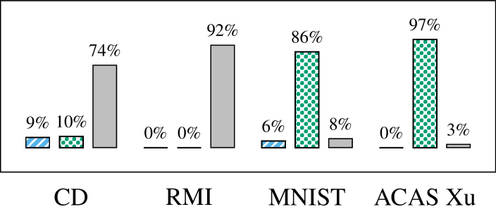
(a) Which is faster in terms of runtime?

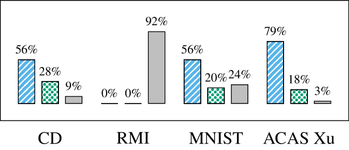
(b) Which is faster in terms of repair steps?

Figure 1: Optimal vs. Early-Exit Verifier. We plot how frequently repair using the optimal verifier  or the early-exit verifier  is faster in terms of (1(a)) runtime and (1(b)) repair steps. Grey bars  depict how frequently both approaches are equally fast. We consider two runtimes equal when they deviate by at most $30$ seconds. We use four different datasets: CollisionDetection (CD), integer datasets (RMI), MNIST and ACAS Xu. Gaps to $100\text{\,}\frac{\mathrm{\char 37\relax}}{}$ are due to failing repairs.

4.6 Early-Exit Verifiers

From a verification perspective, verifiers are not required to find most-violating counterexamples. Instead, it suffices to find any counterexample if one exists. In this section, we show that using just any counterexample is not sufficient for Algorithm 1 to terminate, even for linear regression models. Consider a modification of Algorithm 1, where we only search for a feasible point of $V_{N}$ with a negative objective value instead of the global minimum. This corresponds to using an early-exit verifier during repair. The following proposition demonstrates that this modification can lead to non-termination.

Proposition 4.5 (Non-Termination for Early-Exit Verifiers).

Algorithm 1 modified to use an early-exit verifier is not guaranteed to terminate for $J,f_{\mathrm{Sat}},\NN:\mathbb{R}\to\mathbb{R}$, where $J(\bm{\theta})=|\bm{\theta}|$, $f_{\mathrm{Sat}}(\mathbf{y})=\mathbf{y}$, $\NN(\mathbf{x})=\bm{\theta}-\mathbf{x}$, and $\mathcal{X}_{\varphi}=[0,1]$.

Assume that the early-exit verifier generates the sequence $\textstyle\mathbf{x}^{(N)}=\frac{1}{2}-\frac{1}{N+2}$. This leads to non-termination of Algorithm 1. The detailed proof of Proposition 4.5 is contained in Appendix A.5.

This result concludes our theoretical investigation. In the following section, we research empirical aspects of Algorithm 1, including the practical implications of the above result on using early-exit verifiers during repair.

5 Experiments

Optimal verifiers that compute most-violating counterexamples are theoretically advantageous but not widely available (Strong et al., 2021). Conversely, early-exit verifiers that produce plain counterexamples without further qualifications are readily available (Katz et al., 2019; Bak et al., 2020; Tran et al., 2020; Zhang et al., 2022b; Ferrari et al., 2022), but are theoretically disadvantageous, as apparent from Section 4.6. In this section, we empirically compare the effects of using most-violating counterexamples and sub-optimal counterexamples — as produced by early-exit verifiers and falsifiers — for repair. Additionally, we apply our insights from Section 4.3 for repairing linear regression models. Appendix D contains additional experimental results. Our experiments address the following questions regarding counterexample-guided repair:

1. How does repair using an early-exit verifier compare quantitatively to repair using an optimal verifier?

2. What quantitative advantages does it provide to use falsifiers during repair?

3. Can we surpass existing repair algorithms for linear regression models using our theoretical insights?

In our experiments, we repair an MNIST (LeCun et al., 1998) image classification network, ACAS Xu aircraft control networks (Julian et al., 2018; Katz et al., 2017), a CollisionDetection (Ehlers, 2017) particle dynamics network, and integer dataset Recursive Model Indices (RMIs) (Tan et al., 2021) for database indexing. RMIs contain two stages: a first-stage neural network and several second-stage linear regression models. We collect $50$ repair instances for MNIST, $34$ for ACAS Xu, $100$ for CollisionDetection, $50$ for RMI first-stage networks and $100$ for RMI second-stage models. A detailed description of all datasets, networks and specifications is contained in Appendix B.

For repair, we make use of an early-exit verifier, an optimal verifier, and the BIM falsifier (Kurakin et al., 2017; Madry et al., 2018). To obtain an optimal verifier, we modify the ERAN verifier (Singh et al., 2022) to compute most-violating counterexamples. This is described in Appendix B.1. We use the modified ERAN verifier both as the early-exit and as the optimal verifier. We use the SpecRepair counterexample-removal algorithm (Bauer-Marquart et al., 2022) unless otherwise noted. Our implementation and hardware are documented in Appendix B.4. Our source code is available at https://github.com/sen-uni-kn/specrepair.

5.1 Optimal vs. Early Exit Verifier

To evaluate how repair using an early-exit verifier compares to repair using an optimal verifier, we run repair using both verifiers for CollisionDetection, MNIST, ACAS Xu, and the RMI first-stage networks.

Figure 1 depicts which verifier leads to repair fastest. The figure shows this both for the absolute runtime of repair and the number of repair steps. For the larger MNIST and ACAS Xu networks, we observe that repair using the early-exit verifier requires less runtime in most cases. Regarding the number of repair steps, we observe the opposite trend. Here, the optimal verifier yields repair in fewer repair steps more often than not. The additional runtime cost of computing most-violating counterexamples offsets the advantage in repair steps. For the smaller CollisionDetection network and the RMI first stage networks, we primarily observe that only infrequently repair using one verifier outperforms using the other by more than $30$ seconds. While there is no variation regarding the number of repair steps for the Integer Dataset RMIs, Figure 1(b) shows the same trend for CollisionDetection as for ACAS Xu and MNIST.

5.2 Using Falsifiers for Repair

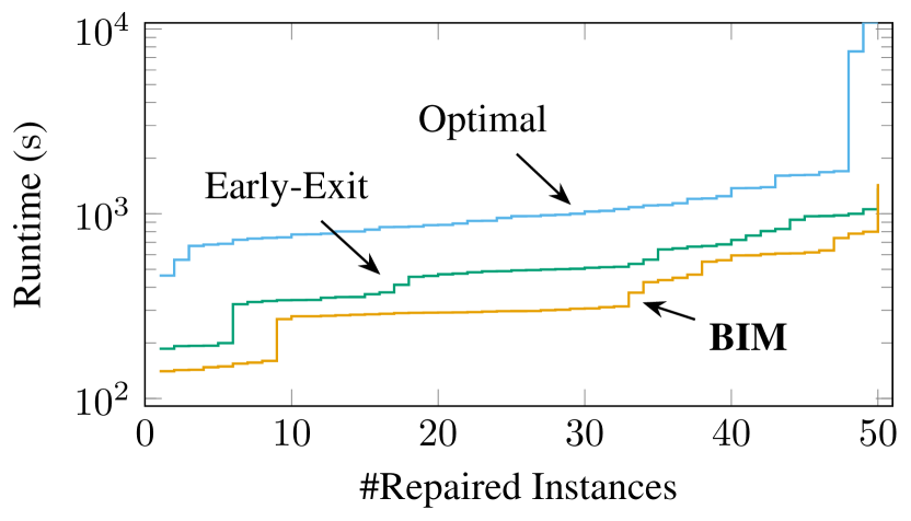
Figure 2: Repair using Falsifiers. We plot the number of repaired MNIST instances that individually require less than a certain runtime. We plot this for repair using BIM , only the optimal verifier  and only the early-exit verifier .

Falsifiers are sound but incomplete counterexample searchers that specialise in finding violations fast. In this section, we study how falsifiers can speed up repair. For this purpose, we repair an MNIST network using the BIM (Kurakin et al., 2017; Madry et al., 2018) falsifier that we describe in Section 3.3. We start repair by searching counterexamples using BIM. Only when BIM fails to produce further counterexamples we turn to the early-exit verifier. Ideally, we would want that the verifier is invoked only once to prove specification satisfaction. Practically, often several additional repair steps have to be performed using the verifier.

Figure 2 summarises the results of our experiment. We see that using BIM can significantly accelerate repair of the MNIST network, demonstrating the potential of falsifiers for repair. BIM is an order of magnitude faster than the early-exit verifier, yet it can find counterexamples with a larger violation. Thus, BIM can sometimes provide the repair step advantage of the optimal verifier at a much smaller cost. Appendix D.1 contains further experiments on using falsifiers for repair.

5.3 Repairing Linear Regression Models

Table 3: Repairing Linear Regression Models. We report the success rates of repairing RMI second-stage linear regression models for two specifications with different error bounds $\varepsilon$. The success rates include models that already satisfy their specification.

	Success Rate
Algorithm	$\varepsilon=100$	$\varepsilon=150$
Ouroboros ∗	$30\text{\,}\frac{\mathrm{\char 37\relax}}{}$	$77\text{\,}\frac{\mathrm{\char 37\relax}}{}$
SpecRepair ⋆	$58\text{\,}\frac{\mathrm{\char 37\relax}}{}$	$94\text{\,}\frac{\mathrm{\char 37\relax}}{}$
Quadratic Programming	$\mathbf{72}\,\textbf{\%}$	$\mathbf{97}\,\textbf{\%}$

^∗ Tan et al. (2021)  ^⋆ Bauer-Marquart et al. (2022)

Our theoretical investigation into the repair of linear regression models in Section 4.3 provides interesting insights that can be used to create a repair algorithm for linear regression models based on quadratic programming. In this section, we describe this algorithm and compare it to the Ouroboros (Tan et al., 2021) and SpecRepair (Bauer-Marquart et al., 2022) repair algorithms. Both Ouroboros and SpecRepair are counterexample-guided repair algorithms. The linear regression models we repair are the second-stage models of several integer dataset RMIs.

Insights into Repairing Linear Regression Models We recall from Section 4.3 that for repairing a linear regression model to conform to a linear specification, the most-violating counterexample for a property is always located at one of the vertices of the property’s input set. This implies two conclusions for repairing the second-stage RMI models:

1. To verify a linear regression model, it suffices to evaluate it on the vertices of the input set. This provides us with an analytical solution of the verification problem $V$. As the input of the RMI second-stage models is one-dimensional, we only have to check property violation for two points per property.

2. Since we can analytically solve $V$, we can rewrite $R^{\prime}$ from Equation (7) using, for RMI second-stage models, two constraints per property. The two constraints correspond to evaluating the satisfaction function for the two vertices of the property input set. We obtain an equivalent formulation of the repair problem $R$ from Equation (6) with a finite number of constraints.

Repair using Quadratic Programming Conclusion b) provides an equivalent formulation of the repair problem $R$ with finitely many linear constraints. We train and repair the second-stage models using MSE. Since MSE is a convex quadratic function and all constraints are linear, it follows that the repair problem is a quadratic program (Boyd & Vandenberghe, 2014). This allows for applying a quadratic programming solver to repair the linear regression models directly. We use Gurobi (Gurobi Optimization, LLC, 2021) and report the results for repairing linear regression models using this method under the name Quadratic Programming.

Table 3 summarises the results of repairing the second-stage RMI linear regression models. Our new Quadratic Programming repair algorithm achieves the highest success rate, outperforming Ouroboros and SpecRepair. In fact, due to solving the repair problem directly, Quadratic Programming is guaranteed to produce the optimal repaired model whenever repair is possible. Our implementation of the different algorithms does not allow for a fair runtime comparison, but we remark that the runtime of Quadratic Programming is competitive in our experiments.

6 Conclusion

In this paper, we prove termination of counterexample-guided repair for linear regression models, linear classifiers and single ReLU neurons, assuming linear specifications. We disprove termination for repairing neural networks when the specification has an unbounded input set. As our results show, our methodology of viewing repair as robust optimisation is useful for studying the theoretical properties of counterexample-guided repair. Empirically, we find that both early-exit verifiers and falsifiers allow achieving repair and can give speed advantages. For repairing linear regression models, we surpass existing approaches by designing a novel repair algorithm using our theoretical insights. Overall, we believe that robust optimisation provides a rich arsenal of useful tools for studying and advancing repair, both theoretically and practically.

Future Work Theorems 4.3 and 4.4 provide sufficient conditions for termination of Algorithm 1. Deriving sufficient conditions that are closer to neural network repair is an interesting direction for future work, as is deriving necessary conditions for termination. Another direction for future work is studying different classes of verifiers beyond optimal and early-exit verifiers. Further sufficient conditions, necessary conditions, and a more refined taxonomy of verifiers could provide insights into why, practically, Algorithm 1 terminates even when using early-exit verifiers.

Appendix A Proofs

This section contains the full proofs of all our propositions and theorems.

A.1 Proposition 4.1

Proof of Proposition 4.1.

Assume Algorithm 1 has terminated after $\overline{N}$ iterations for some robust program $R$. Since Algorithm 1 has terminated, we know that $\min V_{\overline{N}}\geq 0$. Hence, $\bm{\theta}^{(\overline{N}-1)}$ is feasible for $R$. As $\bm{\theta}^{(\overline{N}-1)}$ also minimises ${C\!\!\>R}_{\overline{N}-1}$, which is a relaxation of $R$, it follows that $\bm{\theta}^{(\overline{N}-1)}$ minimises $R$.

This proof is independent of whether we search for a local minimiser or a global minimiser of $R$. Therefore, Proposition 4.1 holds regardless of the type of minimiser of $R$ that we are interested in.

A.2 Proposition 4.2

For proving Proposition 4.2, we first prove non-termination for a simplified version of the network in Proposition 4.2. This simplified version serves as a lemma for proving Proposition 4.2.

Lemma A.1.

Algorithm 1 does not terminate for $J:\mathbb{R}\to\mathbb{R}$, $f_{\mathrm{Sat}}:\mathbb{R}^{2}\to\mathbb{R}$ and $\NN:\mathbb{R}\to\mathbb{R}^{2}$ where $J(\bm{\theta})=\NN(0)_{1}$, $f_{\mathrm{Sat}}(\mathbf{y})=\mathbf{y}_{2}+\mathbf{y}_{1}-1$, $\mathcal{X}_{\varphi}=\mathbb{R}$, and

$${\NN(\mathbf{x})}={\left[\begin{pmatrix}-\bm{\theta}\\ \bm{\theta}-\mathbf{x}\end{pmatrix}\right]}^{+}\!\!\!\!\!\;,$$ (14)

where ${\left[x\right]}^{+}=\max(0,x)$ denotes the ReLU.

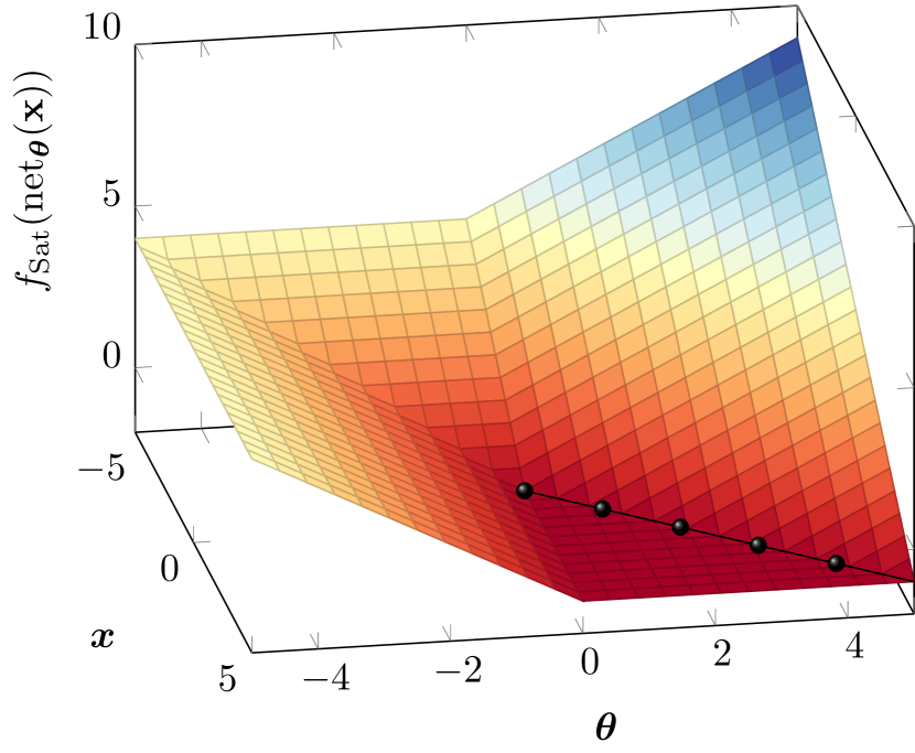
(a) Setting of Proposition 4.2

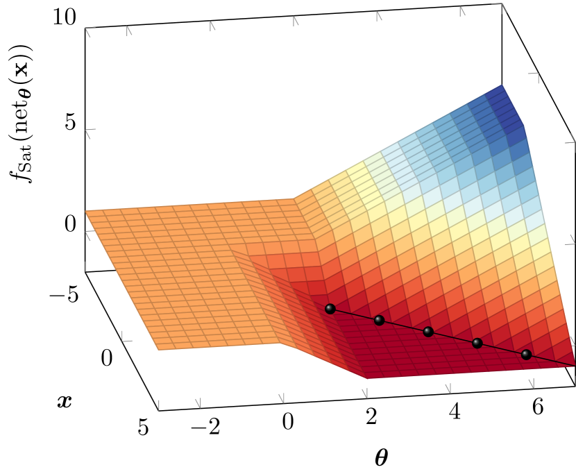
(b) FCNN Variant from Example 1

Figure 3: Constraint Visualisations for Non-Termination Proofs. We visualise the function $f_{\mathrm{Sat}}(\NN(\mathbf{x}))$ from Proposition 4.2 and for the FCNN variant from Example 1. In both cases, the parameter iterates $\bm{\theta}^{(N)}$ and the counterexamples $\mathbf{x}^{(N)}$ diverge to $\infty$ along the dark-red flat surface where the $f_{\mathrm{Sat}}$ value is negative. This divergence implies non-termination of Algorithm 1. The black line  represents an example sequence of diverging parameter and counterexample iterates.

The network $\NN$ in Lemma A.1 corresponds to the network from Proposition 4.2 with $\bm{\theta}_{1}=-1$. This leads to a one-dimensional input and a one-dimensional parameter space. Because of this, we can visualise the optimisation landscape that underlies repairing $\NN$. This visualisation is insightful for the proof of non-termination. Therefore, before we begin the proof of Lemma A.1, we first give an intuition for the proof using Figure 3(a). The core of the proof is that Algorithm 1 generates parameter iterates $\bm{\theta}^{(N)}$ and counterexamples $\mathbf{x}^{(N)}$ that lie on the dark-red flat surface of Figure 3(a), where $f_{\mathrm{Sat}}$ is negative. The combination of $f_{\mathrm{Sat}}$ and the objective function $J$ that prefers non-negative $\bm{\theta}^{(N)}$ leads to $\bm{\theta}^{(N)}\geq 0$ for every $N\in\mathbb{N}$. As there is always a new counterexample $\mathbf{x}^{(N)}$ for every $\bm{\theta}^{(N-1)}\geq 0$, Algorithm 1 does not terminate.

Proof of Lemma A.1.

Let $J$, $f_{\mathrm{Sat}}$, $\NN$ and $\mathcal{X}_{\varphi}$ be as in Lemma A.1. Assembled into a repair problem, they yield

$$R:\left\{\!\begin{array}[]{cl}\underset{\bm{\theta}\in\mathbb{R}}{\text{minimise}}&{\left[-\bm{\theta}\right]}^{+}\\ \text{subject to}&{\left[\bm{\theta}-\mathbf{x}\right]}^{+}+{\left[-\bm{\theta}\right]}^{+}-1\geq 0\quad\forall\mathbf{x}\in\mathbb{R}.\end{array}\right.$$ (15)

We now show that Algorithm 1 does not terminate when applied to $R$. The problem ${C\!\!\>R}_{0}$ is minimising $J(\bm{\theta})={\left[-\bm{\theta}\right]}^{+}$ without constraints. The minimiser of $J$ is not unique, but all minimisers satisfy $\bm{\theta}^{(0)}\geq 0$. Let $\bm{\theta}^{(0)}\geq 0$ be such a minimiser.

Searching for the global minimiser $\mathbf{x}^{(1)}$ of $V_{1}$, we find that this minimiser is non-unique as well. However, all minimisers satisfy $\mathbf{x}^{(1)}\geq\bm{\theta}^{(0)}$. This follows since any minimiser of

$$g{\left(\mathbf{x},\bm{\theta}^{(0)}\right)}={\left[\bm{\theta}^{(0)}-\mathbf{x}\right]}^{+}+{\left[-\bm{\theta}^{(0)}\right]}^{+}-1$$ (16)

minimises $\textstyle{\left[\bm{\theta}^{(0)}-\mathbf{x}\right]}^{+}$ as the remaining terms of Equation (16) are constant regarding $\mathbf{x}$. The observation $\mathbf{x}^{(1)}\geq\bm{\theta}^{(0)}$ applies analogously for later repair steps. Therefore, $\mathbf{x}^{(N)}\geq\bm{\theta}^{(N-1)}$.

For any further repair step, we find that all non-negative feasible points $\bm{\theta}$ of ${C\!\!\>R}_{N}$ satisfy

$$\bm{\theta}\geq\max{\left(\mathbf{x}^{(1)},\ldots,\mathbf{x}^{(N)}\right)}+1.$$ (17)

This follows because $\textstyle g{\left(\mathbf{x}^{(i)},\bm{\theta}\right)}\geq 0$ has to hold for all $i\in\{1,\ldots,N\}$ for $\bm{\theta}$ to be feasible for ${C\!\!\>R}_{N}$. Now, if $\bm{\theta}\geq 0$, we have

$$g{\left(\mathbf{x}^{(i)},\bm{\theta}\right)}={\left[\bm{\theta}-\mathbf{x}^{(i)}\right]}^{+}+{\left[-\bm{\theta}\right]}^{+}-1={\left[\bm{\theta}-\mathbf{x}^{(i)}\right]}^{+}-1\geq 0,$$ (18)

for all $i\in\{1,\ldots,N\}$. We see that Equation (18) is satisfied for all $i\in\{1,\ldots,N\}$ only if $\bm{\theta}$ is larger than the largest $\mathbf{x}^{(i)}$ by at least one. This yields equivalence of Equations (18) and (17).

As Equation (17) always has a solution, there always exists a positive feasible point for ${C\!\!\>R}_{N}$. Now, due to $J$, any minimiser $\bm{\theta}^{(N)}$ of ${C\!\!\>R}_{N}$ is positive and hence satisfies Equation (17). Putting these results together, we obtain

$$\bm{\theta}^{(0)} \geq 0$$ (19a)

$$\mathbf{x}^{(N)} \geq\bm{\theta}^{(N-1)}$$ (19b)

$$\bm{\theta}^{(N)} \geq\mathbf{x}^{(N)}+1.$$ (19c)

Inspecting Equation (15) closely reveals that no positive value $\bm{\theta}$ is feasible for $R$ as there always exists an $\mathbf{x}\geq\bm{\theta}$. However, it follows from Equations (19) that the iterate $\bm{\theta}^{(N)}$ of Algorithm 1 is always positive and thus never feasible for $R$. Since feasibility for $R$ is the criterion for Algorithm 1 to terminate, it follows that Algorithm 1 does not terminate for this repair problem.

Remark A.2.

We might be willing to accept non-termination for problems without a minimiser. However, $R$ from Equation (15) has a minimiser. We have already seen in the proof of Lemma A.1 that all positive $\bm{\theta}$ are infeasible for $R$. Similarly, all $\bm{\theta}\in(-1,0]$ are infeasible. However, all $\bm{\theta}\leq-1$ are feasible as

$${\left[\bm{\theta}-\mathbf{x}\right]}^{+}+{\left[-\bm{\theta}\right]}^{+}-1\geq{\left[-\bm{\theta}\right]}^{+}-1\geq 0,$$ (20)

for any $\mathbf{x}\in\mathbb{R}$. For negative $\bm{\theta}$, $J$ prefers larger values. Because of this, the only minimiser of $R$ is $\bm{\theta}^{\dagger}=-1$. Indeed, Algorithm 1 not only fails to terminate but also moves further and further away from the optimal solution.

We now prove Proposition 4.2 using Lemma A.1. As will become clear during the proof, the divergence for Lemma A.1 transfers to Proposition 4.2.

Proof of Proposition 4.2.

Let $J$, $f_{\mathrm{Sat}}$, $\NN$ and $\mathcal{X}_{\varphi}$ be as in Proposition 4.2. The repair problem is

$$R:\left\{\!\begin{array}[]{cl}\underset{\bm{\theta}\in\mathbb{R}}{\text{minimise}}&{\left[\bm{\theta}_{1}\bm{\theta}_{2}\right]}^{+}\\ \text{subject to}&{\left[\bm{\theta}_{1}\mathbf{x}+\bm{\theta}_{2}\right]}^{+}+{\left[\bm{\theta}_{1}\bm{\theta}_{2}\right]}^{+}-1\geq 0\quad\forall\mathbf{x}\in\mathbb{R}.\end{array}\right.$$ (21)

To show that Algorithm 1 is not guaranteed to terminate for $R$, we now construct an execution of Algorithm 1 that does not terminate. We first consider ${C\!\!\>R}_{0}$, which is minimising $J$ without constraints. Choosing $\bm{\theta}_{1}=-1$ and $\bm{\theta}_{2}\geq 0$ yields a local minimiser of $J$, since $\textstyle J{\left(\bm{\theta}\right)}=0$, which is the global minimum of $J$. Assuming $\bm{\theta}_{2}^{(0)}\geq 0$ and $\bm{\theta}_{1}^{(0)}=-1$, we now show that there is an execution of Algorithm 1, such that

$$\forall N\in\mathbb{N}_{0}:\bm{\theta}_{1}^{(N)}=-1\wedge\bm{\theta}_{2}^{(N)}\geq 0$$ (22)

As $\bm{\theta}_{1}=-1$ recreates the neural network from Lemma A.1, Proposition 4.2 follows from Lemma A.1 when Equation (22) holds for some execution. In the proof of Lemma A.1, we have already shown that there exists a $\bm{\theta}^{(N)}$ satisfying Equation (22) that is feasible for ${C\!\!\>R}_{N}$. Since $\textstyle J{\left(\bm{\theta}^{(N)}\right)}=0$ for any $\bm{\theta}^{(N)}$ satisfying Equation (22), there exist such parameters that are a local (in fact global) minimiser of ${C\!\!\>R}_{N}$. Therefore, Algorithm 1 is not guaranteed to terminate when repairing the neural network in Proposition 4.2, as there exists an execution of Algorithm 1 that does not terminate.

Remark A.3.

While the proof of Proposition 4.2 constructs an execution that does not terminate, the example in Proposition 4.2 also permits executions that terminate. In the following, we discuss different executions of Algorithm 1, including the executions that terminate. Beyond the execution constructed in the proof of Proposition 4.2, all executions with

$$\forall N\in\mathbb{N}_{0}:\bm{\theta}_{1}<0\wedge\bm{\theta}_{2}\geq 0$$ (23)

fail to terminate. Such executions may, however, converge to a solution $\bm{\theta}_{1}=0$, $\bm{\theta}_{2}\geq 1$. While still failing to terminate, they do not diverge. Values of $\bm{\theta}_{1}>0$ lead to non-termination, analogously to the case where $\bm{\theta}_{1}<0$. Also in this case, Algorithm 1 may converge to a solution with $\bm{\theta}_{1}=0$. There also exist executions where Algorithm 1 terminates, namely when it chooses $\bm{\theta}_{1}=0$ at some point during its execution. Choosing $\bm{\theta}_{1}=0$ is a valid choice, as it yields local minimisers of $J$ and allows removing any set of counterexamples. Therefore, for the example in Proposition 4.2, it is possible that Algorithm 1 terminates, but there is no guarantee.

Regarding the plausibility of non-terminating executions, we first remark that it is reasonable to obtain $\bm{\theta}^{(0)}_{1}\neq 0$, as neural network training is unlikely to reach $\bm{\theta}^{(0)}_{1}=0$ exactly. Regarding the plausibility of the choice of local minimisers of ${C\!\!\>R}_{N}$, we consider different concrete counterexample-removal algorithms.

• Gradient-based techniques (Pulina & Tacchella, 2010; Goodfellow et al., 2015; Dong et al., 2021; Tan et al., 2021; Bauer-Marquart et al., 2022) are unable to remove counterexamples for Proposition 4.2, as $f_{\mathrm{Sat}}$ does not provide information on improving property violation through its gradient. This is because the region where the most violating counterexamples are located is flat. Therefore, these techniques fail to remove counterexamples, which makes it impossible to study the termination of Algorithm 1.

• For SMT-based techniques (Goldberger et al., 2020), the choice of the local minimum $\bm{\theta}^{(N)}$ depends on the heuristics applied by the SMT solver. The SMT solver may choose to increase only one parameter, leading to a non-terminating execution, such as the one constructed in the proof of Proposition 4.2.

A.2.1 Example 1

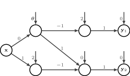
Figure 4: Fully-Connected Neural Network Variant of Proposition 4.2. This Figure visualises Equation (11). Empty nodes represent single ReLU neurons. Edge labels between nodes contain the network weights. Where edges are omitted, the corresponding weights are zero. Biases are written next to the incoming edge above the ReLU neurons.

Figure 4 visualises the FCNN from Example 1 The proof of non-termination for this FCNN is analogous to the proof of Lemma A.1. Figure 3(b) visualises $f_{\mathrm{Sat}}{\left(\NN(\mathbf{x})\right)}$ for the FCNN from Equation (11). Comparison with Figure 3(a) reveals that the key aspects of $f_{\mathrm{Sat}}{\left(\NN(\mathbf{x})\right)}$ for the FCNN are identical to Lemma A.1, except for being shifted. Most notably, there also exists a flat surface with a negative $f_{\mathrm{Sat}}$ value. As $J$ also prefers non-negative $\bm{\theta}$ in this example, Algorithm 1 diverges here as well.

A.3 Theorem 4.3

Proof of Theorem 4.3.

We prove termination of Algorithm 1 for $R$ from Theorem 4.3. Optimality then follows from Proposition 4.1. Let $g:\mathbb{R}^{p}\times\mathbb{R}^{n}\to\mathbb{R}$ be linear in the second argument. Let $\mathcal{X}_{\varphi}$ be a closed convex polytope. Given this, every $V_{N}$ is a linear program and all $V_{N}$ share the same feasible set $\mathcal{X}_{\varphi}$. Because $V_{N}$ is a linear program, its minimiser coincides with one of the vertices of the feasible set $\mathcal{X}_{\varphi}$.

It follows that $\forall N\in\mathbb{N}:\mathbf{x}^{(N)}\in\mathrm{vert}{\left(\mathcal{X}_{\varphi}\right)}$, where $\mathrm{vert}{\left(\mathcal{X}_{\varphi}\right)}$ are the vertices of $\mathcal{X}_{\varphi}$. Because $\mathrm{vert}{\left(\mathcal{X}_{\varphi}\right)}$ is finite, at some repair step $\overline{N}$ of Algorithm 1, we obtain a minimiser that we already encountered in a previous repair step. Let $\tilde{N}$ be this previous repair step, such that $\mathbf{x}^{(\tilde{N})}=\mathbf{x}^{(\overline{N})}$. Since $\bm{\theta}^{(\overline{N}-1)}$ is feasible for ${C\!\!\>R}_{\overline{N}-1}$, it satisfies

$$0\leq g{\left(\bm{\theta}^{(\overline{N}-1)},\mathbf{x}^{(\tilde{N})}\right)}=g{\left(\bm{\theta}^{(\overline{N}-1)},\mathbf{x}^{(\overline{N})}\right)}=f_{\mathrm{Sat}}{\left(\NN[\bm{\theta}^{(\overline{N}-1)}]{\left(\mathbf{x}^{(\overline{N})}\right)}\right)}.$$ (24)

As this is the termination criterion of Algorithm 1, the algorithm terminates in repair step $\overline{N}$.

A.4 Theorem 4.4

We first formally introduce element-wise monotonous functions. Informally, element-wise monotone functions are monotone in each argument, all other arguments being fixed at some value.

Definition A.4 (Element-Wise Monotone).

A function $f:\mathcal{X}\to\mathbb{R}$, $\mathcal{X}\subseteq\mathbb{R}^{n}$, is element-wise monotone if

$$\forall i\in\{1,\ldots,n\}:\forall\mathbf{x}\in\mathcal{X}:{{\left.f\right|}_{\mathcal{X}\cap\left(\{\mathbf{x}_{1}\}\times\cdots\times\{\mathbf{x}_{i-1}\}\times\mathbb{R}\times\{\mathbf{x}_{i+1}\}\times\cdots\times\{\mathbf{x}_{n}\}\right)}}\ \text{is monotone}.$$ (25)

Remark A.5.

Affine transformations of element-wise monotone functions maintain element-wise monotonicity. This directly follows from affine transformations maintaining monotonicity.

Element-wise monotone functions can be monotonically increasing and decreasing in the same element but only for different values of the remaining elements. Examples of element-wise monotone functions include the single neurons $\textstyle{\left[{\mathbf{w}^{\mkern-1.5mu\mathsf{T}}}\mathbf{x}+\mathbf{b}\right]}^{+}$ and $\textstyle\sigma{\left({\mathbf{w}^{\mkern-1.5mu\mathsf{T}}}\mathbf{x}+\mathbf{b}\right)}$, where ${\left[x\right]}^{+}=\max(0,x)$ is the ReLU function and $\textstyle\sigma(x)=\frac{1}{1+e^{-x}}$ is the sigmoid function. These functions are also continuous.

In Theorem 4.4, we make an assumption on the global minimisers that Algorithm 1 prefers when there are multiple global minimisers. In the proof of Lemma A.6, we show that the assumption in Theorem 4.4 is a weak assumption. In particular, we show that it is easy to construct a global minimiser of $V_{N}$ that is a vertex of $\mathcal{X}_{\varphi}$ given any global minimiser of $V_{N}$. Lemma A.6 is a preliminary result for proving Theorem 4.4.

Lemma A.6 (Optimal Vertices).

Let $R$, $g$ and $\mathcal{X}_{\varphi}$ be as in Theorem 4.4. Then, for every $N\in\mathbb{N}$ there is $\tilde{\mathbf{x}}^{(N)}\in\mathrm{vert}{\left(\mathcal{X}_{\varphi}\right)}$ that globally minimises $V_{N}$, where $\mathrm{vert}{\left(\mathcal{X}_{\varphi}\right)}$ denotes the set of vertices of $\mathcal{X}_{\varphi}$.

Proof.

Let $R$, $g$, $\mathcal{X}_{\varphi}$ be as in Lemma A.6. Let $N\in\mathbb{N}$. To prove the lemma we show that a) $V_{N}$ has a minimiser and b) when there is a minimiser of $V_{N}$, some vertex of $\mathcal{X}_{\varphi}$ also minimises $V_{N}$ and has the same $f_{\mathrm{Sat}}$ value.

1. As the feasible set of $V_{N}$ is closed and bounded due to being a hyper-rectangle and the objective function is continuous, $V_{N}$ has a minimiser.

2. Let $\mathbf{x}^{(N)}\in\mathbb{R}^{n}$ be a global minimiser of $V_{N}$. We show that there is a $\tilde{\mathbf{x}}^{(N)}\in\mathrm{vert}{\left(\mathcal{X}_{\varphi}\right)}$ such that $\tilde{\mathbf{x}}^{(N)}$ also minimises $V_{N}$ since

   $$g{\left(\bm{\theta}^{(N-1)},\mathbf{x}^{(N)}\right)}\geq g{\left(\bm{\theta}^{(N-1)},\tilde{\mathbf{x}}^{(N)}\right)}.$$ (26)

   Pick any dimension $i\in\{1,\ldots,n\}$. As $g$ is element-wise monotone, it is non-increasing in one of the two directions along dimension $i$ starting from $\mathbf{x}^{(N)}$. When $\mathbf{x}^{(N)}$ does not already lie on a face of $\mathcal{X}_{\varphi}$ that bounds expansion along the $i$-axis, we walk along the non-increasing direction along dimension $i$ until we reach such a face of $\mathcal{X}_{\varphi}$. As $\mathcal{X}_{\varphi}$ is a hyper-rectangle and, therefore, bounded, it is guaranteed that we reach such a face. We pick the point on the face of $\mathcal{X}_{\varphi}$ as the new $\mathbf{x}^{(N)}$. While keeping dimension $i$ fixed, we repeat the above procedure for a different dimension $j\in\{1,\ldots,n\},i\neq j$. We iterate the procedure over all dimensions always keeping the value of $\mathbf{x}^{(N)}$ in already visited dimensions fixed.

   In every step of this procedure, we restrict ourselves to a lower-dimensional face of $\mathcal{X}_{\varphi}$ as we fix the value in one dimension. Thus, when we have visited every dimension, we have reached a $0$-dimensional face of $\mathcal{X}_{\varphi}$, that is, a vertex. Since we only walked along directions in which $g$ is non-increasing and since $g$ is element-wise monotone, the vertex $\tilde{\mathbf{x}}^{(N)}$ that we obtain satisfies Equation (26). Since $\mathbf{x}^{(N)}$ is a global minimiser, Equation (26) needs to hold with equality.

Together, a) and b) yield that there is always a vertex $\tilde{\mathbf{x}}^{(N)}\in\mathrm{vert}{\left(\mathcal{X}_{\varphi}\right)}$ that globally minimises $V_{N}$.

Proof of Theorem 4.4.

We prove termination with optimality following from Proposition 4.1. Let $R$, $g$, $\mathcal{X}_{\varphi}$ be as in Theorem 4.4. Also, assume that Algorithm 1 prefers vertices of $\mathcal{X}_{\varphi}$ as global minimisers of $V_{N}$. From Lemma A.6 we know that there is always a vertex of $\mathcal{X}_{\varphi}$ that minimises $V_{N}$. From the proof of Lemma A.6 we also know that it is easy to find such a vertex given any global minimiser of $V_{N}$. As Algorithm 1 always chooses vertices of $\mathcal{X}_{\varphi}$ under our assumption, there is only a finite set of minimisers $\mathbf{x}^{(N)}$, as a hyper-rectangle has only finitely many vertices. Given this, termination follows analogously to the proof of Theorem 4.3.

A.5 Proposition 4.5

Proof of Proposition 4.5.

Let $J$, $f_{\mathrm{Sat}}$, $\NN$ and $\mathcal{X}_{\varphi}$ be as in Proposition 4.5. When inserting these into Equation (6), we obtain the repair problem

$$R:\left\{\!\begin{array}[]{cl}\underset{\bm{\theta}\in\mathbb{R}}{\text{minimise}}&|\bm{\theta}|\\ \text{subject to}&\bm{\theta}-\mathbf{x}\geq 0\quad\forall\mathbf{x}\in[0,1].\end{array}\right.$$ (27)

Assume the early-exit verifier generates the sequence $\mathbf{x}^{(N)}=\frac{1}{2}-\frac{1}{N+2}$ as long as these points are counterexamples for $\NN[\bm{\theta}^{(N-1)}]$. Otherwise, let it produce $\mathbf{x}^{(N)}=1$, the global minimum of all $V_{N}$.

Minimising $J$ without constraints yields $\bm{\theta}^{(0)}=0$. The point $\mathbf{x}^{(1)}=\frac{1}{2}-\frac{1}{3}$ is a valid result of the early-exit verifier for $V_{1}$, as it is a counterexample. We observe that the constraint

$$f_{\mathrm{Sat}}(\NN(\mathbf{x}))=\bm{\theta}-\mathbf{x}\geq 0$$ (28)

is tight when $\bm{\theta}=\mathbf{x}$. Smaller $\bm{\theta}$ violate the constraint. Since $J$ prefers values of $\bm{\theta}$ closer to zero, it always holds for any minimiser of ${C\!\!\>R}_{N}$ that

$$\bm{\theta}^{(N)}=\max{\left(\mathbf{x}^{(1)},\ldots,\mathbf{x}^{(N)}\right)}=\mathbf{x}^{(N)}.$$ (29)

The last equality is due to the construction of the points returned by the early-exit verifier. However, for these values of $\bm{\theta}^{(N)}$, $\textstyle\frac{1}{2}-\frac{1}{N+2}$ always remains a valid product of the early-exit verifier for $V_{N}$. Thus we obtain,

$$\bm{\theta}^{(N)}=\mathbf{x}^{(N)}=\frac{1}{2}-\frac{1}{N+2}.$$ (30)

The minimiser of $R$ is $\bm{\theta}^{\dagger}=1$. However, $\bm{\theta}^{(N)}$ does not converge to this point but to the infeasible $\lim_{N\to\infty}\bm{\theta}^{(N)}=\frac{1}{2}$. Since the iterates $\bm{\theta}^{(N)}$ always remain infeasible for $R$, the modified Algorithm 1 never terminates.

Appendix B Experiment Design

In our experiments, we repair an MNIST (LeCun et al., 1998) network, ACAS Xu networks (Katz et al., 2017), a CollisionDetection (Ehlers, 2017) network, and integer dataset Recursive Model Indices (RMIs) (Tan et al., 2021). For repair, we make use of an early-exit verifier, an optimal verifier, the SpecAttack falsifier (Bauer-Marquart et al., 2022), and the BIM falsifier (Madry et al., 2018; Kurakin et al., 2017). To obtain an optimal verifier, we modify the ERAN verifier (Singh et al., 2022) to compute most-violating counterexamples. We use the modified ERAN verifier both as the early-exit and as the optimal verifier in our experiments, as it supports both exit modes.

In all experiments, we use the SpecRepair counterexample-removal algorithm (Bauer-Marquart et al., 2022) unless otherwise noted. We set up all verifiers and falsifiers to return a single counterexample. For SpecAttack, which produces multiple counterexamples, we select the counterexample with the largest violation. We make this modification to eliminate differences due to some tools returning more counterexamples than others, as we are interested in studying the effects of counterexample quality, not counterexample quantity.

We make our source code available under the Apache 2.0 license at https://github.com/sen-uni-kn/specrepair. Our experimental data is available at https://doi.org/10.5281/zenodo.7938547.

B.1 Modifying ERAN to Compute Most-Violating Counterexamples

The ETH Robustness Verifier for Neural Networks (ERAN) (Singh et al., 2022) combines abstract interpretation with Mixed Integer Linear Programming (MILP) to verify neural networks. For our experiments, we use the DeepPoly abstract interpretation (Singh et al., 2019). ERAN leverages Gurobi (Gurobi Optimization, LLC, 2021) for MILP. To verify properties with low-dimensional input sets having a large diameter, ERAN implements the ReluVal input splitting branch and bound procedure (Wang et al., 2018). We employ this branch and bound procedure only for ACAS Xu.

The Gurobi MILP solver can be configured to stop optimisation when encountering the first point with a negative satisfaction function value below a small threshold. We use this feature for the early-exit mode. To compute most-violating counterexamples, we instead run the MILP solver until achieving optimality.

The input-splitting branch and bound procedure evaluates branches in parallel. In the early-exit mode, the procedure terminates when it finds a counterexample on any branch. As other branches may contain more-violating counterexamples, we search the entire branch and bound tree in the optimal mode.

B.2 Datasets, Networks, and Specifications

Table 4: Network Architectures. In(•) gives the dimension of the network input. Convolutional layers are denoted Conv(out=•, kernel=•, stride=•, pad=•), where out is the number of filters and kernel, stride, and pad are the kernel size, stride, and padding for all spatial dimensions of the layer input. Fully-connected layers are denoted FC(out=•), where out is the number of neurons. [•] × $n$ denotes the $n$-fold repetition of the block in square brackets. RMI stands for the Integer Dataset RMIs.

Dataset	Network Architecture
MNIST	In(1×28×28), Conv(out=8, kernel=3, stride=3, pad=1), ReLU, FC(out=80), ReLU, FC(out=10)
ACAS Xu	In(5), [FC(out=50), ReLU] × 6, FC(out=5)
Collision-Detection	In(6), [FC(out=10), ReLU] × 2, FC(out=2)
RMI, First Stage	In(1), [FC(out=16), ReLU] × 2, FC(out=1)
RMI, Second Stage	In(1), FC(out=1)

We perform experiments with four different datasets. In this section, we introduce the datasets, as well as what networks we repair to conform to which specifications. The network architectures for each dataset are contained in Table 4.

B.2.1 MNIST

The MNIST dataset (LeCun et al., 1998) consists of $70\,000$ labelled images of hand-written Arabic digits. Each image consists of $28\times 28$ pixels. The dataset is split into a training set of $60\,000$ images and a test set of $10\,000$ images. The task is to predict the digit in an image from the image pixel data. We train a small convolutional neural network achieving $97\text{\,}\frac{\mathrm{\char 37\relax}}{}$ test set accuracy ($98$% training set accuracy). Table 4 contains the concrete architecture.

We repair the $L_{\infty}$ adversarial robustness of this convolutional neural network for groups of $25$ input images. These images are randomly sampled from the images in the training set for which the network is not robust. Each robustness property has a radius of $0.03$. Overall, we form $50$ non-overlapping groups of input images. Thus, each repaired network is guaranteed to be locally robust for a different group of $25$ training set images. While specifications of this size are not practically relevant, they make it feasible to perform several ($50$) experiments for each verifier variant. We formally define $L_{\infty}$ adversarial robustness in Appendix C.1.

We train the MNIST network using Stochastic Gradient Descent (SGD) with a mini-batch size of $32$, a learning rate of $0.01$ and a momentum coefficient of $0.9$, training for two epochs. Counterexample-removal uses the same setup, except for using a decreased learning rate of $0.001$ and iterating only for a tenth of an epoch.

B.2.2 ACAS Xu

The ACAS Xu networks (Katz et al., 2017) form a collision avoidance system for aircraft without onboard personnel. Each network receives five sensor measurements that characterise an encounter with another aircraft. Based on these measurements, an ACAS Xu network computes scores for five possible steering directions: Clear of Conflict (maintain course), weak left/right, and strong left/right. The steering direction advised to the aircraft is the output with the minimal score. Each of the $45$ ACAS Xu networks is responsible for another class of encounter scenarios. More details on the system are provided by Julian et al. (2018). Each ACAS Xu network is a fully-connected ReLU network with six hidden layers of $50$ neurons each.

Katz et al. (2017) provide safety specifications for the ACAS Xu networks. Of these specifications, the property $\phi_{2}$ is violated by the largest number of networks. We repair $\phi_{2}$ for all networks violating it, yielding $34$ repair cases. The property $\phi_{2}$ specifies that the score for the Clear of Conflict action is never maximal (least-advised) when the intruder is far away and slow. The precise formal definition of $\phi_{2}$ is given in Appendix C.2.

We repair the ACAS Xu networks following Bauer-Marquart et al. (2022). To replace the unavailable ACAS Xu training data, we randomly sample a training and a validation set and compare with the scores produced by the original network. As a loss function, we use the asymmetric mean square error loss of Julian & Kochenderfer (2019). We repair using the Adam training algorithm (Kingma & Ba, 2015) with a learning rate of $10^{-4}$. We terminate training on convergence, when the loss on the validation set starts to increase, or after at most $500$ iterations.

For assessing the performance of repaired networks, we compare the accuracy and the Mean Absolute Error (MAE) between the predictions of the repaired network and the predictions of the original network on a large grid of inputs, filtering out counterexamples. For all networks, the filtered grid contains more than $24$ million points.

B.2.3 CollisionDetection

The CollisionDetection dataset (Ehlers, 2017) is introduced for evaluating neural network verifiers. The task is to predict whether two particles collide based on their relative position, speed, and turning angles. The training set of $7000$ instances and the test set of $3000$ instances are obtained from simulating particle dynamics for randomly sampled initial configurations. We train a small fully-connected neural network with $20$ neurons on this dataset. The full architecture is given in Table 4.

Similarly to MNIST, we repair the adversarial robustness of this network for 100 non-overlapping groups of ten randomly sampled inputs from the training set. Here we also include inputs that do not violate the specification to gather a sufficient number of groups. Each robustness property has a radius of $0.05$.

The CollisionDetection network is trained for $1000$ iterations using Adam (Kingma & Ba, 2015) with a learning rate of $0.01$. Repair uses Adam with a learning rate of $0.001$, terminating training on convergence or when reaching $5000$ iterations.

B.2.4 Integer Dataset RMIs

Learned index structures replace index structures, such as B-trees, with machine learning models (Kraska et al., 2018). Tan et al. (2021) identify these models as prime candidates for neural network verification and repair due to the strict requirements of their domain and the small size of the models. We use Recursive Model Indices (RMIs) (Kraska et al., 2018) in our experiments. The task of an RMI is to resolve a key to a position in a sorted sequence.

We build datasets, RMIs and specifications following Tan et al. (2021), with the exception that we create models of two sizes. While Tan et al. (2021) build one RMI with a second-stage size of ten, we build ten RMIs with a second-stage size of ten and $50$ RMIs with a second-stage size of $304$. Each RMI is constructed for a different dataset. We create models of two second-stage sizes because the smaller size does not yield unsafe first-stage models, while the larger second-stage size does not yield unsafe second-stage models. However, we want to repair models of both stages. Therefore, when repairing first-stage models in Section 5.2, we repair the first-stage models of the RMIs with second-stage size $304$. In Section 5.3, we repair the second-stage models of the RMIs with second-stage size ten.

Each dataset is a randomly generated integer dataset consisting of a sorted sequence of $190\,000$ integers. The integers are randomly sampled from a uniform distribution with the range $\left[0,10^{6}\right]$. The task is to predict the index of an integer (key) in the sorted sequence.

We build an RMI for each dataset. Each RMI consists of two stages. The first stage contains one neural network. The second stage contains several linear regression models. In our case, the second stage contains either ten or $304$ models. Each dataset is first split into several disjoint blocks, one for each second-stage model. Now, the first-stage network is trained to predict the block an integer key belongs to. The purpose of this model is to select a model from the second stage. Each model of the second stage is responsible for resolving the keys in a block to the position of the key in the sorted sequence. The architectures of the models are given in Table 4.

We train the first-stage model to minimise the Mean Square Error (MSE) between the model predictions and the true blocks. Training uses Adam (Kingma & Ba, 2015) with a learning rate of $0.01$ and a mini-batch size of $512$. For an RMI with a second-stage size of ten, we train for one epoch. For the larger second-stage size of $304$, we train for six epochs.

Minimising the MSE between the positions a second-stage model predicts and the true positions can be solved analytically. We use the analytic solution for training the second-stage models. In Section 5.3, we compare with Ouroboros (Tan et al., 2021) that also uses the analytic solution. SpecRepair (Bauer-Marquart et al., 2022) can not make use of the analytic solution. Instead, it repairs second-stage models using gradient descent with a learning rate of $10^{-13}$, running for $150$ iterations.

The specifications for the RMIs are error bounds on the predictions of each model. For a first-stage neural network, the specification is that it may not deviate by more than one valid block from the true block. The specification for a second-stage model consists of one property for each key in the target block and one for all other keys that the first stage assigns to the second-stage model. The property for a key $k_{i}$ specifies that the prediction for all keys between the previous key $k_{i-1}$ and the next key $k_{i+1}$ in the dataset may not deviate by more than $\varepsilon$ from the position for $k_{i}$. We use two sets of specifications, one with $\varepsilon=100$ and one with $\varepsilon=150$. According to Tan et al. (2021), the specifications express a guaranteed error bound for looking up both existing and non-existing keys. The formal definitions of the specifications are given in Appendix C.3.

As the original Ouroboros implementation is not publicly available, we reimplement Ouroboros, including creating integer dataset RMIs. To roughly estimate whether our reimplementation is faithful, we can examine the average size of the specifications for the second-stage models for the RMIs with second-stage size ten. As these specifications include keys that are wrongly assigned to a second-stage model, they can serve for quantifying the accuracy of the first-stage models. The specifications that we obtain for these models have a similar average size as reported by Tan et al. (2021) ($19\,426$ properties). This indicates that our reimplementation is faithful.

B.3 Repair Algorithms

Except for Section 5.3, we exclusively use the SpecRepair counterexample-removal algorithm (Bauer-Marquart et al., 2022) in our experiments. In Section 5.3, we also use the Ouroboros (Tan et al., 2021) repair algorithm and the novel Quadratic Programming repair algorithm. Additionally, we leverage different falsifiers for repair. This section introduces these tools.

Both Ouroboros and SpecRepair are counterexample-guided repair algorithms. Ouroboros performs repair by augmenting the training set with counterexamples and retraining the linear regression models using an analytic solution. SpecRepair uses the $L_{1}$ penalty function method (Nocedal & Wright, 2006). We use SpecRepair with a decreased initial penalty weight of $2^{-4}$ and a satisfaction constant of $10^{-4}$. We do not limit the number of repair steps a repair algorithm may perform, except for Section 5.3. Here, we perform at most two repair steps for SpecRepair. For Ouroboros, we perform up to five repair steps following Tan et al. (2021).

The Quadratic Programming repair algorithm from Section 5.3 is exact. That is, we obtain an infeasible problem if and only if the linear regression model can not satisfy the specification and otherwise obtain the optimal repaired regression model. To mitigate floating point issues, we require the satisfaction function to be at least $10^{-2}$ in Equation (6) instead of requiring it to be just non-negative. That corresponds to applying a satisfaction constant as in SpecRepair (Bauer-Marquart et al., 2022).

We run SpecAttack Bauer-Marquart et al. (2022) using Sequential Least SQuares Programming (SLSQP) as network gradients are available. Following Carlini & Wagner (2017), we run BIM (Kurakin et al., 2017; Madry et al., 2018) with Adam (Kingma & Ba, 2015) as optimiser. BIM performs local optimisation ten times from different random starting points.

B.4 Implementation and Hardware

We build upon SpecRepair (Bauer-Marquart et al., 2022) for our experiments, leveraging the modified ERAN. SpecRepair and ERAN are implemented in Python. SpecRepair is based on PyTorch (Paszke et al., 2019). For repairing linear regression models, we also use an ERAN-based Python reimplementation of Ouroboros (Tan et al., 2021). The original Ouroboros implementation is not publicly available. The quadratic programming repair algorithm for linear regression models is implemented in Python and leverages Gurobi (Gurobi Optimization, LLC, 2021).

All experiments were conducted on Ubuntu 2022.04.1 LTS machines using Python 3.8. The ACAS Xu, CollisionDetection and Integer Dataset RMI experiments were run on a compute server with an Intel Xeon E5–2580 v4 2.4GHz CPU (28 cores) and 1008GB of memory. The MNIST experiments were run on a GPU compute server with an AMD Ryzen Threadripper 3960X 24-Core Processor and 252GB of memory, utilising an NVIDIA RTX A6000 GPU with 48GB of memory.

We limit the execution time for repairing each ACAS Xu network and each MNIST specification to three hours. For CollisionDetection and the Integer Dataset RMIs, we use a shorter timeout of one hour. Except for ACAS Xu, whenever we report runtimes, we repeat all experiments ten times and report the median runtime from these runs. This way, we obtain more accurate runtime measurements that are necessary for interpreting runtime differences below one minute. For ACAS Xu, the runtime differences are sufficiently large for all but one network, so that we can faithfully compare different counterexample searchers without repeating the experiments.

Appendix C Specifications

In this section, we formally define the specifications used throughout this paper.

C.1 $\mathbf{L}_{\bm{\infty}}$ Adversarial Robustness

Adversarial robustness is a specification for classifiers capturing that small perturbations of an input may not change the classification. For $L_{\infty}$ adversarial robustness, the input set is an $L_{\infty}$ ball (a hyper-rectangle).

Assume the input space has $n$ dimensions and there are $m$ classes. Furthermore, assume the classifier produces a score for each class so that the classifier has $m$ outputs. Also, assume the classification is the class with the largest score. Let $\mathcal{D}\subset\mathbb{R}^{n}\times\{1,\ldots,m\}$ be the set of labelled inputs for which we want to specify adversarial robustness. Then, the $L_{\infty}$ adversarial robustness specification with radius $\varepsilon$ is

$$\Phi ={\{\varphi(\mathbf{x},c)\mid(\mathbf{x},c)\in\mathcal{D}\}}$$ (31a)

$$\varphi(\mathbf{x},c) =\left(\left\{\mathbf{x}^{\prime}\mid\mathbf{x}^{\prime}\in\mathbb{R}^{n},{\lVert\mathbf{x}^{\prime}-\mathbf{x}\rVert}_{\infty}\leq\varepsilon\right\},\left\{\mathbf{y}\;\left|\;\mathbf{y}\in\mathbb{R}^{m},\bigwedge_{i=1}^{m}\mathbf{y}_{i}\leq\mathbf{y}_{c}\right.\right\}\right).$$ (31b)

The SpecRepair satisfaction function (Bauer-Marquart et al., 2022) for a property $\varphi(\mathbf{x},c)$ is

$$f_{\mathrm{Sat}}(\mathbf{y})=\min_{i=1}^{m}\mathbf{y}_{c}-\mathbf{y}_{i}.$$ (32)

Equivalently, we can split up each property into several properties with just one linear constraint, yielding a linear specification. We describe this in Section C.3.

C.2 ACAS Xu $\bm{\phi}_{\mathbf{2}}$

This safety specification consists of a single property. The property $\phi_{2}$ of Katz et al. (2017) is

$$\phi_{2}=\left([55947.691,\infty]\times\mathbb{R}^{2}\times[1145,\infty]\times[-\infty,60],\left\{\mathbf{y}\;\left|\;\mathbf{y}\in\mathbb{R}^{5},\bigvee_{i=1}^{5}\mathbf{y}_{1}\leq\mathbf{y}_{i}\right.\right\}\right).$$ (33)

The output set expresses that Clear-of-Conflict is not the maximal score, or, in other words, is not least advised. The input set of this property is unbounded, but each ACAS Xu network has a bounded input domain. Intersected with one of the input domains, we obtain a closed input set for the property. The SpecRepair satisfaction function for $\phi_{2}$ is

$$f_{\mathrm{Sat}}(\mathbf{y})=\max_{i=1}^{m}\mathbf{y}_{i}-\mathbf{y}_{1}.$$ (34)

C.3 Integer Dataset RMI Error Bounds

For an RMI, the specification of a first-stage model is that it may not deviate by more than one valid block from the true block a key resides in. Let $[l_{1},u_{1}],[l_{2},u_{2}],\ldots,[l_{K},u_{K}]$ be the blocks of the RMI, where $K\in\{10,304\}$ is the number of blocks. Then, the specification of the first-stage model is

$$\Phi ={\{\varphi_{i}\}}_{i=1}^{K}$$ (35a)

$$\varphi_{i} =\left([l_{i},u_{i}],[\max(1,i-1),\min(i+1,K)]\right)\quad\forall i\in\{1,\ldots,K\}.$$ (35b)

The specification of a second-stage model contains one property for each key $k_{i}$ that is in the model’s target block or is assigned to the model by the first-stage model. Let $\mathcal{K}\subset\mathbb{N}$ be the indices of keys that are in the model’s block or assigned to it. Each property expresses that the predictions for all keys between the previous key $k_{i-1}$ and the next key $k_{i+1}$ deviate by at most $\varepsilon\in\{100,150\}$ from the true position $p_{i}$ of $k_{i}$. When there is no previous or next key in the dataset, we use the key itself as bound. Therefore, $k_{0}=k_{1}$ and $k_{$190\,001$}=k_{$190\,000$}$. Now, the second-stage specification is

$$\Phi ={\{\varphi_{i}\}}_{i\in\mathcal{K}}$$ (36a)

$$\varphi_{i} =\left([\min(k_{i-1}+1,k_{i}),\max(k_{i+1}-1,k_{i})],[p_{i}-\varepsilon,p_{i}+\varepsilon]\right).$$ (36b)

The output sets of these properties are hyper-rectangles. In the SpecRepair property format, one-dimensional hyper-rectangles correspond to a conjunction of two linear constraints. A conjunction of multiple linear constraints does not yield an affine satisfaction function, as SpecRepair uses a minimum to encode conjunctions. This is illustrated by Equation (32). To obtain a linear specification, we can split each property into two properties, such that each property only has one linear constraint. Using this alternative formulation, the specification of a second-stage model is

$$\Phi ={\{\varphi_{i}\}}_{i\in\mathcal{K}}\cup{\{\psi_{i}\}}_{i\in\mathcal{K}}$$ (37a)

$$\varphi_{i} =\left([\min(k_{i-1}+1,k_{i}),\max(k_{i+1}-1,k_{i})],\{\mathbf{y}\mid\mathbf{y}\in\mathbb{R},\mathbf{y}\geq p_{i}-\varepsilon\}\right)$$ (37b)

$$\psi_{i} =\left([\min(k_{i-1}+1,k_{i}),\max(k_{i+1}-1,k_{i})],\{\mathbf{y}\mid\mathbf{y}\in\mathbb{R},\mathbf{y}\leq p_{i}+\varepsilon\}\right).$$ (37c)

This formulation yields the affine SpecRepair satisfaction functions $f_{\mathrm{Sat}}(\mathbf{y})=\mathbf{y}-p_{i}-\varepsilon$ for the property $\varphi_{i}$ and $f_{\mathrm{Sat}}(\mathbf{y})=p_{i}+\varepsilon-\mathbf{y}$ for $\psi_{i}$. As the input set of each property is a hyper-rectangle, $\Phi$ from Equation (37) is a linear specification.

Appendix D Additional Experimental Results

In this section, we report additional experimental results. This includes additional results on using falsifiers for repair and an overview of the success rates and repaired network performance when using different verifiers and falsifiers for repair. For comparison with earlier work, we report our full ACAS Xu results in Section D.3.

A Note on Failing Repairs We witness several failing repairs in our experiments. These are either due to timeout or due to failing counterexample-removal. There are no indications of non-termination regarding Algorithm 1 itself in these failing repairs. In other words, we do not observe exceedingly high repair step counts. This holds true both for the optimal verifier, for which termination remains an open question, and the early-exit verifier, for which we disprove termination in Section 4.6.

D.1 Using Falsifiers for Repair

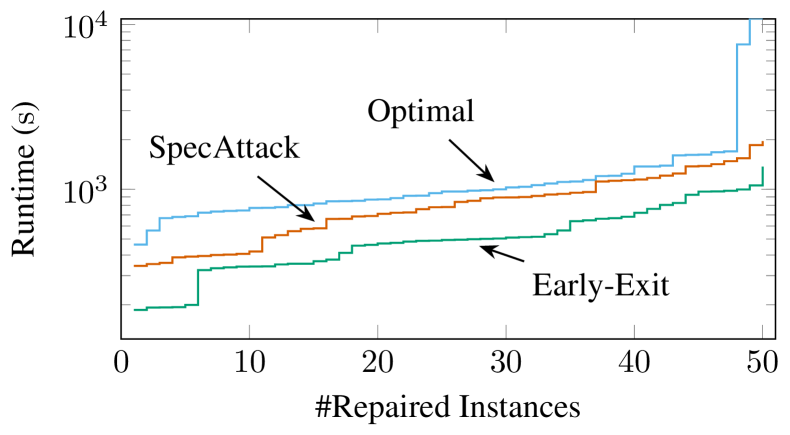
(a) MNIST

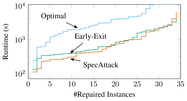
(b) ACAS Xu

Figure 5: Repair using Falsifiers. We plot the number of repaired instances that individually require less than a certain runtime. We plot this for repair using SpecAttack , only the optimal verifier  and only the early-exit verifier . Both experiments use a timeout of three hours. Runtimes are given on a logarithmic scale.

In this section, we report additional results on repair using falsifiers. To study the advantages of falsifiers for repair, we repair an MNIST network and the ACAS Xu networks using the SpecAttack (Bauer-Marquart et al., 2022) and BIM (Kurakin et al., 2017; Madry et al., 2018) falsifiers. We outline the approach of the BIM falsifier in Section 3.3. We start repair by searching counterexamples using one of the falsifiers. Only when the falsifier fails to produce further counterexamples we turn to the early-exit verifier. Ideally, we would want that the verifier is invoked only once to prove specification satisfaction. Practically, often several additional repair steps have to be performed using the verifier.

For ACAS Xu, we observe that BIM generally fails to find counterexamples. Therefore, we only report using SpecAttack for ACAS Xu. For the small CollisionDetection and Integer Dataset networks, the verifier is already comparably fast, so neither BIM nor SpecAttack can provide a runtime advantage. We also evaluated combining falsifiers with the optimal verifier, but this does not improve upon using the early-exit verifier.

SpecAttack Figure 5 summarises our results for repairing the MNIST network and the ACAS Xu networks using SpecAttack. For the MNIST network, using SpecAttack is inferior to using only the early-exit verifier. In our experiments, SpecAttack provides no significant runtime advantage for generating counterexamples over the early-exit verifier and tends to compute counterexamples with a smaller violation. SpecAttack’s runtime scales well with the network size but exponentially in the input dimension. Thus, it is not surprising that it provides no advantage for our MNIST network, which is tiny compared to state-of-the-art image classification networks.

For ACAS Xu, we would expect that SpecAttack outperforms using only the early-exit verifier more clearly than apparent from Figure 5. Here, SpecAttack’s runtime is an order of magnitude faster than the runtime of the early-exit verifier. SpecAttack can also provide an advantage in repair steps in many cases. However, at times using SpecAttack also increases the number of repair steps. Additionally, SpecAttack sometimes makes the final invocations of the early-exit verifier more costly than when only the verifier is used.

Additional Results on BIM The results of our experiments using BIM on MNIST are summarised in Figure 2. We already discussed that BIM can significantly accelerate repair. For MNIST, repair using BIM is the fastest method in $70\text{\,}\frac{\mathrm{\char 37\relax}}{}$ of the repair cases, compared to $26\text{\,}\frac{\mathrm{\char 37\relax}}{}$ for only the early-exit verifier, $2\text{\,}\frac{\mathrm{\char 37\relax}}{}$ for SpecAttack and $0\text{\,}\frac{\mathrm{\char 37\relax}}{}$ for only the optimal verifier. In $2\text{\,}\frac{\mathrm{\char 37\relax}}{}$ of the cases, the runtime of the two best variants is within $30$ seconds. The breakdown of which method is the fastest for each repair case shows that the picture is not as clear as we may wish it to be — BIM provides a significant runtime advantage in $70\text{\,}\frac{\mathrm{\char 37\relax}}{}$ of the cases, but in $26\text{\,}\frac{\mathrm{\char 37\relax}}{}$ of the cases using only the early-exit verifier is faster.

Our experiments using falsifiers demonstrate that they can give a substantial runtime advantage to repair, but they also show that speeding up repair traces back to more intricate properties beyond just falsifier speed. Understanding these properties better is a promising future research direction for designing better falsifiers for repair.

D.2 Success Rates and Repaired Network Performance

Table 5: Experiments: Success Rates. The success rates when repairing the ACAS Xu, MNIST, and CollisionDetection networks and integer dataset RMI first-stage models using the different verifiers and falsifiers. For ACAS Xu, BIM is not included as it is unable to discover counterexamples for these networks.

	Success Rate
Dataset	Optimal	Early-Exit	BIM	SpecAttack
ACAS Xu	$82.5\text{\,}\frac{\mathrm{\char 37\relax}}{}$	$100.0\text{\,}\frac{\mathrm{\char 37\relax}}{}$	–	$100.0\text{\,}\frac{\mathrm{\char 37\relax}}{}$
MNIST	$96.0\text{\,}\frac{\mathrm{\char 37\relax}}{}$	$100.0\text{\,}\frac{\mathrm{\char 37\relax}}{}$	$100.0\text{\,}\frac{\mathrm{\char 37\relax}}{}$	$100.0\text{\,}\frac{\mathrm{\char 37\relax}}{}$
Integer Datasets	$92.0\text{\,}\frac{\mathrm{\char 37\relax}}{}$	$92.0\text{\,}\frac{\mathrm{\char 37\relax}}{}$	$94.0\text{\,}\frac{\mathrm{\char 37\relax}}{}$	$90.0\text{\,}\frac{\mathrm{\char 37\relax}}{}$
CollisionDetection	$90.0\text{\,}\frac{\mathrm{\char 37\relax}}{}$	$90.0\text{\,}\frac{\mathrm{\char 37\relax}}{}$	$89.0\text{\,}\frac{\mathrm{\char 37\relax}}{}$	$88.0\text{\,}\frac{\mathrm{\char 37\relax}}{}$

Table 6: Experiments: Median Accuracy. The median repaired network accuracy when repairing the ACAS Xu, MNIST, and CollisionDetection networks and integer dataset RMI first-stage models using the different verifiers and falsifiers. We report the test set accuracy for MNIST and CollisionDetection and the training set accuracy for the integer dataset RMIs. For ACAS Xu, we report the accuracy for recreating the predictions of the original network for a large grid of inputs, as described in Appendix B.2. We report the median accuracy among the cases where repair is successful for all verifiers and falsifiers. For ACAS Xu, BIM is not included as it is unable to discover counterexamples for these networks.

	Median Accuracy
Dataset	Optimal	Early-Exit	BIM	SpecAttack
ACAS Xu	$99.6\text{\,}\frac{\mathrm{\char 37\relax}}{}$	$99.6\text{\,}\frac{\mathrm{\char 37\relax}}{}$	–	$99.6\text{\,}\frac{\mathrm{\char 37\relax}}{}$
MNIST	$97.4\text{\,}\frac{\mathrm{\char 37\relax}}{}$	$97.5\text{\,}\frac{\mathrm{\char 37\relax}}{}$	$97.4\text{\,}\frac{\mathrm{\char 37\relax}}{}$	$97.5\text{\,}\frac{\mathrm{\char 37\relax}}{}$
Integer Datasets	$90.9\text{\,}\frac{\mathrm{\char 37\relax}}{}$	$90.9\text{\,}\frac{\mathrm{\char 37\relax}}{}$	$90.0\text{\,}\frac{\mathrm{\char 37\relax}}{}$	$91.0\text{\,}\frac{\mathrm{\char 37\relax}}{}$
CollisionDetection	$89.8\text{\,}\frac{\mathrm{\char 37\relax}}{}$	$90.2\text{\,}\frac{\mathrm{\char 37\relax}}{}$	$90.0\text{\,}\frac{\mathrm{\char 37\relax}}{}$	$89.9\text{\,}\frac{\mathrm{\char 37\relax}}{}$

Table 5 summarises the success rates of repairing MNIST, ACAS Xu, and CollisionDetection networks and Integer Dataset RMI first-stage models using different verifiers and falsifiers. For the large MNIST and ACAS Xu networks, the early-exit verifier enables repair in some cases where repair using the optimal verifier fails due to timeout. Regarding the use of falsifiers, there are minor variations for the Integer Dataset RMIs and CollisionDetection. These differences are due to failing repairs. Here, the counterexample removal procedure is unable to remove all counterexamples provided by, for example, the optimal verifier, while it succeeds for another set of counterexamples.

Table 6 summarises the performance of the repaired networks. We only observe minimal variations regarding the performance. Using the early-exit verifier slightly outperforms the optimal verifiers on MNIST and CollisionDetection. The impact of BIM and SpecAttack is inconsistent across datasets. We recommend fine-tuning the initial penalty weight to the counterexample violation magnitude instead of using a different counterexample searcher to increase repaired network performance.

D.3 ACAS Xu

Table 7: Detailed ACAS Xu Results. Opt. and E.E denote repair using the optimal and the early-exit verifier, respectively. Sp.A. denotes repair using SpecAttack and the early-exit verifier. The symbol 1.2✓ denotes successful repair, while 1.05⍾ denotes timeout. Both accuracy and Mean Absolute Error (MAE) compare the predictions of the repaired network with the predictions of the initial faulty network for a large grid of inputs. More details on this are provided in Appendix B.2.

		Status			Accuracy			MAE
Spec.	Model	Opt.	E.E.	Sp.A.	Opt.	E.E.	Sp.A.	Opt.	E.E.	Sp.A.
$\phi_{2}$	$N_{2,1}$	1.2✓	1.2✓	1.2✓	$99.6\text{\,}\frac{\mathrm{\char 37\relax}}{}$	$99.4\text{\,}\frac{\mathrm{\char 37\relax}}{}$	$99.6\text{\,}\frac{\mathrm{\char 37\relax}}{}$	$0.10$	$0.15$	$0.11$
$\phi_{2}$	$N_{2,2}$	1.05⍾	1.2✓	1.2✓	–	$99.2\text{\,}\frac{\mathrm{\char 37\relax}}{}$	$99.1\text{\,}\frac{\mathrm{\char 37\relax}}{}$	–	$0.18$	$0.22$
$\phi_{2}$	$N_{2,3}$	1.2✓	1.2✓	1.2✓	$99.7\text{\,}\frac{\mathrm{\char 37\relax}}{}$	$99.7\text{\,}\frac{\mathrm{\char 37\relax}}{}$	$99.7\text{\,}\frac{\mathrm{\char 37\relax}}{}$	$0.09$	$0.10$	$0.11$
$\phi_{2}$	$N_{2,4}$	1.2✓	1.2✓	1.2✓	$99.7\text{\,}\frac{\mathrm{\char 37\relax}}{}$	$99.5\text{\,}\frac{\mathrm{\char 37\relax}}{}$	$99.8\text{\,}\frac{\mathrm{\char 37\relax}}{}$	$0.08$	$0.11$	$0.08$
$\phi_{2}$	$N_{2,5}$	1.05⍾	1.2✓	1.2✓	–	$99.4\text{\,}\frac{\mathrm{\char 37\relax}}{}$	$99.3\text{\,}\frac{\mathrm{\char 37\relax}}{}$	–	$0.11$	$0.11$
$\phi_{2}$	$N_{2,6}$	1.2✓	1.2✓	1.2✓	$99.6\text{\,}\frac{\mathrm{\char 37\relax}}{}$	$99.5\text{\,}\frac{\mathrm{\char 37\relax}}{}$	$99.5\text{\,}\frac{\mathrm{\char 37\relax}}{}$	$0.12$	$0.11$	$0.10$
$\phi_{2}$	$N_{2,7}$	1.05⍾	1.2✓	1.2✓	–	$99.5\text{\,}\frac{\mathrm{\char 37\relax}}{}$	$14.5\text{\,}\frac{\mathrm{\char 37\relax}}{}$	–	$0.17$	$0.16$
$\phi_{2}$	$N_{2,8}$	1.2✓	1.2✓	1.2✓	$99.6\text{\,}\frac{\mathrm{\char 37\relax}}{}$	$99.6\text{\,}\frac{\mathrm{\char 37\relax}}{}$	$99.7\text{\,}\frac{\mathrm{\char 37\relax}}{}$	$0.12$	$0.15$	$0.13$
$\phi_{2}$	$N_{2,9}$	1.2✓	1.2✓	1.2✓	$99.9\text{\,}\frac{\mathrm{\char 37\relax}}{}$	$99.8\text{\,}\frac{\mathrm{\char 37\relax}}{}$	$99.8\text{\,}\frac{\mathrm{\char 37\relax}}{}$	$0.17$	$0.14$	$0.14$
$\phi_{2}$	$N_{3,1}$	1.2✓	1.2✓	1.2✓	$99.0\text{\,}\frac{\mathrm{\char 37\relax}}{}$	$99.3\text{\,}\frac{\mathrm{\char 37\relax}}{}$	$99.4\text{\,}\frac{\mathrm{\char 37\relax}}{}$	$0.22$	$0.14$	$0.17$
$\phi_{2}$	$N_{3,2}$	1.2✓	1.2✓	1.2✓	$99.9\text{\,}\frac{\mathrm{\char 37\relax}}{}$	$99.8\text{\,}\frac{\mathrm{\char 37\relax}}{}$	$99.8\text{\,}\frac{\mathrm{\char 37\relax}}{}$	$0.08$	$0.09$	$0.13$
$\phi_{2}$	$N_{3,4}$	1.2✓	1.2✓	1.2✓	$99.6\text{\,}\frac{\mathrm{\char 37\relax}}{}$	$99.6\text{\,}\frac{\mathrm{\char 37\relax}}{}$	$99.6\text{\,}\frac{\mathrm{\char 37\relax}}{}$	$0.11$	$0.13$	$0.08$
$\phi_{2}$	$N_{3,5}$	1.2✓	1.2✓	1.2✓	$99.5\text{\,}\frac{\mathrm{\char 37\relax}}{}$	$99.5\text{\,}\frac{\mathrm{\char 37\relax}}{}$	$99.5\text{\,}\frac{\mathrm{\char 37\relax}}{}$	$0.08$	$0.10$	$0.08$
$\phi_{2}$	$N_{3,6}$	1.2✓	1.2✓	1.2✓	$99.8\text{\,}\frac{\mathrm{\char 37\relax}}{}$	$99.8\text{\,}\frac{\mathrm{\char 37\relax}}{}$	$99.7\text{\,}\frac{\mathrm{\char 37\relax}}{}$	$0.05$	$0.06$	$0.06$
$\phi_{2}$	$N_{3,7}$	1.2✓	1.2✓	1.2✓	$99.6\text{\,}\frac{\mathrm{\char 37\relax}}{}$	$99.6\text{\,}\frac{\mathrm{\char 37\relax}}{}$	$99.7\text{\,}\frac{\mathrm{\char 37\relax}}{}$	$0.09$	$0.08$	$0.08$
$\phi_{2}$	$N_{3,8}$	1.2✓	1.2✓	1.2✓	$99.6\text{\,}\frac{\mathrm{\char 37\relax}}{}$	$99.6\text{\,}\frac{\mathrm{\char 37\relax}}{}$	$99.7\text{\,}\frac{\mathrm{\char 37\relax}}{}$	$0.13$	$0.10$	$0.11$
$\phi_{2}$	$N_{3,9}$	1.05⍾	1.2✓	1.2✓	–	$97.5\text{\,}\frac{\mathrm{\char 37\relax}}{}$	$97.5\text{\,}\frac{\mathrm{\char 37\relax}}{}$	–	$0.19$	$0.18$
$\phi_{2}$	$N_{4,1}$	1.2✓	1.2✓	1.2✓	$99.8\text{\,}\frac{\mathrm{\char 37\relax}}{}$	$99.8\text{\,}\frac{\mathrm{\char 37\relax}}{}$	$99.8\text{\,}\frac{\mathrm{\char 37\relax}}{}$	$0.10$	$0.07$	$0.10$
$\phi_{2}$	$N_{4,3}$	1.2✓	1.2✓	1.2✓	$99.6\text{\,}\frac{\mathrm{\char 37\relax}}{}$	$99.6\text{\,}\frac{\mathrm{\char 37\relax}}{}$	$99.5\text{\,}\frac{\mathrm{\char 37\relax}}{}$	$0.09$	$0.08$	$0.13$
$\phi_{2}$	$N_{4,4}$	1.2✓	1.2✓	1.2✓	$99.7\text{\,}\frac{\mathrm{\char 37\relax}}{}$	$99.6\text{\,}\frac{\mathrm{\char 37\relax}}{}$	$99.7\text{\,}\frac{\mathrm{\char 37\relax}}{}$	$0.11$	$0.15$	$0.09$
$\phi_{2}$	$N_{4,5}$	1.2✓	1.2✓	1.2✓	$99.6\text{\,}\frac{\mathrm{\char 37\relax}}{}$	$99.5\text{\,}\frac{\mathrm{\char 37\relax}}{}$	$99.5\text{\,}\frac{\mathrm{\char 37\relax}}{}$	$0.09$	$0.07$	$0.12$
$\phi_{2}$	$N_{4,6}$	1.05⍾	1.2✓	1.2✓	–	$99.5\text{\,}\frac{\mathrm{\char 37\relax}}{}$	$99.6\text{\,}\frac{\mathrm{\char 37\relax}}{}$	–	$0.13$	$0.11$
$\phi_{2}$	$N_{4,7}$	1.05⍾	1.2✓	1.2✓	–	$99.2\text{\,}\frac{\mathrm{\char 37\relax}}{}$	$99.2\text{\,}\frac{\mathrm{\char 37\relax}}{}$	–	$0.17$	$0.18$
$\phi_{2}$	$N_{4,8}$	1.2✓	1.2✓	1.2✓	$99.4\text{\,}\frac{\mathrm{\char 37\relax}}{}$	$99.3\text{\,}\frac{\mathrm{\char 37\relax}}{}$	$99.5\text{\,}\frac{\mathrm{\char 37\relax}}{}$	$0.08$	$0.08$	$0.09$
$\phi_{2}$	$N_{4,9}$	1.2✓	1.2✓	1.2✓	$96.5\text{\,}\frac{\mathrm{\char 37\relax}}{}$	$96.4\text{\,}\frac{\mathrm{\char 37\relax}}{}$	$96.5\text{\,}\frac{\mathrm{\char 37\relax}}{}$	$0.16$	$0.14$	$0.13$
$\phi_{2}$	$N_{5,1}$	1.2✓	1.2✓	1.2✓	$99.7\text{\,}\frac{\mathrm{\char 37\relax}}{}$	$99.5\text{\,}\frac{\mathrm{\char 37\relax}}{}$	$99.6\text{\,}\frac{\mathrm{\char 37\relax}}{}$	$0.12$	$0.13$	$0.09$
$\phi_{2}$	$N_{5,2}$	1.2✓	1.2✓	1.2✓	$99.7\text{\,}\frac{\mathrm{\char 37\relax}}{}$	$99.7\text{\,}\frac{\mathrm{\char 37\relax}}{}$	$99.7\text{\,}\frac{\mathrm{\char 37\relax}}{}$	$0.08$	$0.07$	$0.08$
$\phi_{2}$	$N_{5,3}$	1.2✓	1.2✓	1.2✓	$99.9\text{\,}\frac{\mathrm{\char 37\relax}}{}$	$99.9\text{\,}\frac{\mathrm{\char 37\relax}}{}$	$99.9\text{\,}\frac{\mathrm{\char 37\relax}}{}$	$0.04$	$0.04$	$0.04$
$\phi_{2}$	$N_{5,4}$	1.2✓	1.2✓	1.2✓	$99.7\text{\,}\frac{\mathrm{\char 37\relax}}{}$	$99.7\text{\,}\frac{\mathrm{\char 37\relax}}{}$	$99.7\text{\,}\frac{\mathrm{\char 37\relax}}{}$	$0.10$	$0.07$	$0.10$
$\phi_{2}$	$N_{5,5}$	1.2✓	1.2✓	1.2✓	$99.8\text{\,}\frac{\mathrm{\char 37\relax}}{}$	$99.7\text{\,}\frac{\mathrm{\char 37\relax}}{}$	$99.8\text{\,}\frac{\mathrm{\char 37\relax}}{}$	$0.10$	$0.13$	$0.11$
$\phi_{2}$	$N_{5,6}$	1.2✓	1.2✓	1.2✓	$99.6\text{\,}\frac{\mathrm{\char 37\relax}}{}$	$99.5\text{\,}\frac{\mathrm{\char 37\relax}}{}$	$99.5\text{\,}\frac{\mathrm{\char 37\relax}}{}$	$0.13$	$0.11$	$0.11$
$\phi_{2}$	$N_{5,7}$	1.2✓	1.2✓	1.2✓	$99.3\text{\,}\frac{\mathrm{\char 37\relax}}{}$	$99.3\text{\,}\frac{\mathrm{\char 37\relax}}{}$	$99.5\text{\,}\frac{\mathrm{\char 37\relax}}{}$	$0.17$	$0.14$	$0.11$
$\phi_{2}$	$N_{5,8}$	1.2✓	1.2✓	1.2✓	$99.6\text{\,}\frac{\mathrm{\char 37\relax}}{}$	$99.4\text{\,}\frac{\mathrm{\char 37\relax}}{}$	$99.5\text{\,}\frac{\mathrm{\char 37\relax}}{}$	$0.13$	$0.12$	$0.13$
$\phi_{2}$	$N_{5,9}$	1.2✓	1.2✓	1.2✓	$99.0\text{\,}\frac{\mathrm{\char 37\relax}}{}$	$98.9\text{\,}\frac{\mathrm{\char 37\relax}}{}$	$99.1\text{\,}\frac{\mathrm{\char 37\relax}}{}$	$0.14$	$0.13$	$0.09$
		28	34	34	$99.6\text{\,}\frac{\mathrm{\char 37\relax}}{}$	$99.5\text{\,}\frac{\mathrm{\char 37\relax}}{}$	$99.6\text{\,}\frac{\mathrm{\char 37\relax}}{}$	$0.10$	$0.11$	$0.11$
		success frequency			median			median

For comparison with the earlier work of Bauer-Marquart et al. (2022), we report our detailed ACAS Xu results in Table 7. Due to improvements in the interaction with the verifier, we are successful more frequently than any method evaluated by Bauer-Marquart et al. (2022). At the same time, we maintain the level of repaired network performance.

References

- Amato et al. (2013) Amato, F., López, A., Peña-Méndez, E. M., Vaňhara, P., Hampl, A., and Havel, J. Artificial neural networks in medical diagnosis. J. Appl. Biomed., 11(2):47–58, 2013. URL https://doi.org/10.2478/v10136-012-0031-x.
- Bak et al. (2020) Bak, S., Tran, H., Hobbs, K., and Johnson, T. T. Improved Geometric Path Enumeration for Verifying ReLU Neural Networks. In CAV (1), volume 12224 of Lecture Notes in Computer Science, pp. 66–96. Springer, 2020. URL https://doi.org/10.1007/978-3-030-53288-8_4.
- Bauer-Marquart et al. (2022) Bauer-Marquart, F., Boetius, D., Leue, S., and Schilling, C. SpecRepair: Counter-Example Guided Safety Repair of Deep Neural Networks. In SPIN, volume 13255 of Lecture Notes in Computer Science, pp. 79–96. Springer, 2022. URL https://doi.org/10.1007/978-3-031-15077-7_5.
- Ben-Tal & Nemirovski (1998) Ben-Tal, A. and Nemirovski, A. Robust Convex Optimization. Math. Oper. Res., 23(4):769–805, 1998. URL https://doi.org/10.1287/moor.23.4.769.
- Ben-Tal et al. (2009) Ben-Tal, A., Ghaoui, L. E., and Nemirovski, A. Robust Optimization, volume 28 of Princeton Series in Applied Mathematics. Princeton University Press, 2009. URL https://doi.org/10.1515/9781400831050.
- Bojarski et al. (2016) Bojarski, M., Testa, D. D., Dworakowski, D., Firner, B., Flepp, B., Goyal, P., Jackel, L. D., Monfort, M., Muller, U., Zhang, J., Zhang, X., Zhao, J., and Zieba, K. End to End Learning for Self-Driving Cars. CoRR, abs/1604.07316, 2016. URL http://arxiv.org/abs/1604.07316.
- Boyd & Vandenberghe (2014) Boyd, S. P. and Vandenberghe, L. Convex Optimization. Cambridge University Press, 2014. URL https://doi.org/10.1017/CBO9780511804441.
- Brown et al. (2020) Brown, T. B., Mann, B., Ryder, N., Subbiah, M., Kaplan, J., Dhariwal, P., Neelakantan, A., Shyam, P., Sastry, G., Askell, A., Agarwal, S., Herbert-Voss, A., Krueger, G., Henighan, T., Child, R., Ramesh, A., Ziegler, D. M., Wu, J., Winter, C., Hesse, C., Chen, M., Sigler, E., Litwin, M., Gray, S., Chess, B., Clark, J., Berner, C., McCandlish, S., Radford, A., Sutskever, I., and Amodei, D. Language Models are Few-Shot Learners. In NeurIPS, 2020. URL https://proceedings.neurips.cc/paper/2020/hash/1457c0d6bfcb4967418bfb8ac142f64a-Abstract.html.
- Bunel et al. (2018) Bunel, R., Turkaslan, I., Torr, P. H. S., Kohli, P., and Mudigonda, P. K. A Unified View of Piecewise Linear Neural Network Verification. In NeurIPS, pp. 4795–4804, 2018. URL https://proceedings.neurips.cc/paper/2018/hash/be53d253d6bc3258a8160556dda3e9b2-Abstract.html.
- Campi & Garatti (2008) Campi, M. C. and Garatti, S. The Exact Feasibility of Randomized Solutions of Uncertain Convex Programs. SIAM J. Optim., 19(3):1211–1230, 2008. URL https://doi.org/10.1137/07069821X.
- Carlini & Wagner (2017) Carlini, N. and Wagner, D. A. Towards Evaluating the Robustness of Neural Networks. In IEEE Symposium on Security and Privacy, pp. 39–57. IEEE Computer Society, 2017. URL https://doi.org/10.1109/SP.2017.49.
- Chen et al. (2020) Chen, J., Jordan, M. I., and Wainwright, M. J. HopSkipJumpAttack: A Query-Efficient Decision-Based Attack. In IEEE Symposium on Security and Privacy, pp. 1277–1294. IEEE, 2020. URL https://doi.org/10.1109/SP40000.2020.00045.
- Cheng et al. (2017) Cheng, C., Nührenberg, G., and Ruess, H. Maximum Resilience of Artificial Neural Networks. In ATVA, volume 10482 of Lecture Notes in Computer Science, pp. 251–268. Springer, 2017. URL https://doi.org/10.1007/978-3-319-68167-2_18.
- Cissé et al. (2017) Cissé, M., Bojanowski, P., Grave, E., Dauphin, Y. N., and Usunier, N. Parseval Networks: Improving Robustness to Adversarial Examples. In ICML, volume 70 of Proceedings of Machine Learning Research, pp. 854–863. PMLR, 2017. URL http://proceedings.mlr.press/v70/cisse17a.html.
- Clarke et al. (2000) Clarke, E. M., Grumberg, O., Jha, S., Lu, Y., and Veith, H. Counterexample-guided abstraction refinement. In CAV, volume 1855 of Lecture Notes in Computer Science, pp. 154–169. Springer, 2000. URL https://doi.org/10.1007/10722167_15.
- Dong et al. (2021) Dong, G., Sun, J., Wang, J., Wang, X., and Dai, T. Towards Repairing Neural Networks Correctly. In QRS, pp. 714–725. IEEE, 2021. URL https://doi.org/10.1109/QRS54544.2021.00081.
- Ehlers (2017) Ehlers, R. Formal Verification of Piece-Wise Linear Feed-Forward Neural Networks. In ATVA, volume 10482 of Lecture Notes in Computer Science, pp. 269–286. Springer, 2017. URL https://doi.org/10.1007/978-3-319-68167-2_19.
- Esfahani et al. (2015) Esfahani, P. M., Sutter, T., and Lygeros, J. Performance Bounds for the Scenario Approach and an Extension to a Class of Non-Convex Programs. IEEE Trans. Autom. Control., 60(1):46–58, 2015. URL https://doi.org/10.1109/TAC.2014.2330702.
- Fawzi et al. (2022) Fawzi, A., Balog, M., Huang, A., Hubert, T., Romera-Paredes, B., Barekatain, M., Novikov, A., R. Ruiz, F. J., Schrittwieser, J., Swirszcz, G., Silver, D., Hassabis, D., and Kohli, P. Discovering faster matrix multiplication algorithms with reinforcement learning. Nat., 610(7930):47–53, 2022. URL https://doi.org/10.1038/s41586-022-05172-4.
- Ferrari et al. (2022) Ferrari, C., Mueller, M. N., Jovanović, N., and Vechev, M. Complete Verification via Multi-Neuron Relaxation Guided Branch-and-Bound. In ICLR, 2022. URL https://openreview.net/forum?id=l_amHf1oaK.
- Fischer et al. (2019) Fischer, M., Balunovic, M., Drachsler-Cohen, D., Gehr, T., Zhang, C., and Vechev, M. T. DL2: Training and Querying Neural Networks with Logic. In ICML, volume 97 of Proceedings of Machine Learning Research, pp. 1931–1941. PMLR, 2019. URL http://proceedings.mlr.press/v97/fischer19a.html.
- Goldberger et al. (2020) Goldberger, B., Katz, G., Adi, Y., and Keshet, J. Minimal Modifications of Deep Neural Networks using Verification. In LPAR, volume 73 of EPiC Series in Computing, pp. 260–278. EasyChair, 2020. URL https://easychair.org/publications/paper/CWhF.
- Goodfellow et al. (2015) Goodfellow, I. J., Shlens, J., and Szegedy, C. Explaining and Harnessing Adversarial Examples. In ICLR (Poster), 2015. URL http://arxiv.org/abs/1412.6572.
- Goodfellow et al. (2016) Goodfellow, I. J., Bengio, Y., and Courville, A. C. Deep Learning. Adaptive computation and machine learning. MIT Press, 2016. URL http://www.deeplearningbook.org/.
- Gowal et al. (2018) Gowal, S., Dvijotham, K., Stanforth, R., Bunel, R., Qin, C., Uesato, J., Arandjelovic, R., Mann, T. A., and Kohli, P. On the Effectiveness of Interval Bound Propagation for Training Verifiably Robust Models. CoRR, abs/1810.12715, 2018. URL http://arxiv.org/abs/1810.12715.
- Guidotti et al. (2019a) Guidotti, D., Leofante, F., Pulina, L., and Tacchella, A. Verification and Repair of Neural Networks: A Progress Report on Convolutional Models. In AI*IA, volume 11946 of Lecture Notes in Computer Science, pp. 405–417. Springer, 2019a. URL https://doi.org/10.1007/978-3-030-35166-3_29.
- Guidotti et al. (2019b) Guidotti, D., Leofante, F., Tacchella, A., and Castellini, C. Improving reliability of myocontrol using formal verification. IEEE Trans. Neural Syst. Rehabilitation Eng., 27(4):564–571, 2019b. URL https://doi.org/10.1109/TNSRE.2019.2893152.
- Gurobi Optimization, LLC (2021) Gurobi Optimization, LLC. Gurobi Optimizer Reference Manual, 2021. URL https://www.gurobi.com.
- Henzinger et al. (2003) Henzinger, T. A., Jhala, R., and Majumdar, R. Counterexample-guided control. In ICALP, volume 2719 of Lecture Notes in Computer Science, pp. 886–902. Springer, 2003. URL https://doi.org/10.1007/3-540-45061-0_69.
- Jha & Seshia (2014) Jha, S. and Seshia, S. A. Are there good mistakes? A theoretical analysis of CEGIS. In SYNT, volume 157 of EPTCS, pp. 84–99, 2014. URL https://doi.org/10.4204/EPTCS.157.10.
- Jorgensen (1997) Jorgensen, C. C. Direct Adaptive Aircraft Control Using Dynamic Cell Structure Neural Networks. Technical report, NASA Ames Research Center, 1997.
- Julian & Kochenderfer (2019) Julian, K. D. and Kochenderfer, M. J. Guaranteeing Safety for Neural Network-Based Aircraft Collision Avoidance Systems. CoRR, abs/1912.07084, 2019. URL http://arxiv.org/abs/1912.07084.
- Julian et al. (2018) Julian, K. D., Kochenderfer, M. J., and Owen, M. P. Deep Neural Network Compression for Aircraft Collision Avoidance Systems. CoRR, abs/1810.04240, 2018. URL http://arxiv.org/abs/1810.04240.
- Katz et al. (2017) Katz, G., Barrett, C. W., Dill, D. L., Julian, K. D., and Kochenderfer, M. J. Reluplex: An Efficient SMT Solver for Verifying Deep Neural Networks. In CAV (1), volume 10426 of Lecture Notes in Computer Science, pp. 97–117. Springer, 2017. URL https://doi.org/10.1007/978-3-319-63387-9_5.
- Katz et al. (2019) Katz, G., Huang, D. A., Ibeling, D., Julian, K., Lazarus, C., Lim, R., Shah, P., Thakoor, S., Wu, H., Zeljic, A., Dill, D. L., Kochenderfer, M. J., and Barrett, C. W. The Marabou Framework for Verification and Analysis of Deep Neural Networks. In CAV (1), volume 11561 of Lecture Notes in Computer Science, pp. 443–452. Springer, 2019. URL https://doi.org/10.1007/978-3-030-25540-4_26.
- Kingma & Ba (2015) Kingma, D. P. and Ba, J. Adam: A Method for Stochastic Optimization. In ICLR, 2015. URL http://arxiv.org/abs/1412.6980.
- Kraska et al. (2018) Kraska, T., Beutel, A., Chi, E. H., Dean, J., and Polyzotis, N. The Case for Learned Index Structures. In SIGMOD Conference, pp. 489–504. ACM, 2018. URL https://doi.org/10.1145/3183713.3196909.
- Kurakin et al. (2017) Kurakin, A., Goodfellow, I. J., and Bengio, S. Adversarial examples in the physical world. In ICLR. OpenReview.net, 2017. URL https://openreview.net/forum?id=HJGU3Rodl.
- LeCun et al. (1998) LeCun, Y., Bottou, L., Bengio, Y., and Haffner, P. Gradient-based learning applied to document recognition. Proc. IEEE, 86(11):2278–2324, 1998. URL https://doi.org/10.1109/5.726791.
- Lomuscio & Maganti (2017) Lomuscio, A. and Maganti, L. An approach to reachability analysis for feed-forward ReLU neural networks. CoRR, abs/1706.07351, 2017. URL http://arxiv.org/abs/1706.07351.
- Madry et al. (2018) Madry, A., Makelov, A., Schmidt, L., Tsipras, D., and Vladu, A. Towards Deep Learning Models Resistant to Adversarial Attacks. In ICLR (Poster). OpenReview.net, 2018. URL https://openreview.net/forum?id=rJzIBfZAb.
- Mirman et al. (2018) Mirman, M., Gehr, T., and Vechev, M. T. Differentiable Abstract Interpretation for Provably Robust Neural Networks. In ICML, volume 80 of Proceedings of Machine Learning Research, pp. 3575–3583. PMLR, 2018. URL http://proceedings.mlr.press/v80/mirman18b.html.
- Müller et al. (2022) Müller, M. N., Brix, C., Bak, S., Liu, C., and Johnson, T. T. The Third International Verification of Neural Networks Competition (VNN-COMP 2022): Summary and Results. CoRR, abs/2212.10376, 2022. URL https://doi.org/10.48550/arXiv.2212.10376.
- Mutapcic & Boyd (2009) Mutapcic, A. and Boyd, S. P. Cutting-set methods for robust convex optimization with pessimizing oracles. Optim. Methods Softw., 24(3):381–406, 2009. URL https://doi.org/10.1080/10556780802712889.
- Nguyen et al. (2017) Nguyen, T., Antonopoulos, T., Ruef, A., and Hicks, M. Counterexample-guided approach to finding numerical invariants. In ESEC/FSE, pp. 605–615. ACM, 2017. URL https://doi.org/10.1145/3106237.3106281.
- Nocedal & Wright (2006) Nocedal, J. and Wright, S. J. Numerical Optimization. Springer, 2 edition, 2006. URL https://doi.org/10.1007/b98874.
- Palma et al. (2021) Palma, A. D., Bunel, R., Desmaison, A., Dvijotham, K., Kohli, P., Torr, P. H. S., and Kumar, M. P. Improved Branch and Bound for Neural Network Verification via Lagrangian Decomposition. CoRR, abs/2104.06718, 2021. URL https://arxiv.org/abs/2104.06718.
- Papernot et al. (2015) Papernot, N., McDaniel, P. D., Jha, S., Fredrikson, M., Celik, Z. B., and Swami, A. The Limitations of Deep Learning in Adversarial Settings. CoRR, abs/1511.07528, 2015. URL http://arxiv.org/abs/1511.07528.
- Paszke et al. (2019) Paszke, A., Gross, S., Massa, F., Lerer, A., Bradbury, J., Chanan, G., Killeen, T., Lin, Z., Gimelshein, N., Antiga, L., Desmaison, A., Köpf, A., Yang, E., DeVito, Z., Raison, M., Tejani, A., Chilamkurthy, S., Steiner, B., Fang, L., Bai, J., and Chintala, S. PyTorch: An Imperative Style, High-Performance Deep Learning Library. In NeurIPS, pp. 8024–8035, 2019. URL https://proceedings.neurips.cc/paper/2019/hash/bdbca288fee7f92f2bfa9f7012727740-Abstract.html.
- Pulina & Tacchella (2010) Pulina, L. and Tacchella, A. An Abstraction-Refinement Approach to Verification of Artificial Neural Networks. In CAV, volume 6174 of Lecture Notes in Computer Science, pp. 243–257. Springer, 2010. URL https://doi.org/10.1007/978-3-642-14295-6_24.
- Raghunathan et al. (2018) Raghunathan, A., Steinhardt, J., and Liang, P. Certified Defenses against Adversarial Examples. In ICLR (Poster). OpenReview.net, 2018. URL https://openreview.net/forum?id=Bys4ob-Rb.
- Reynolds et al. (2015) Reynolds, A., Deters, M., Kuncak, V., Tinelli, C., and Barrett, C. W. Counterexample-guided quantifier instantiation for synthesis in SMT. In CAV (2), volume 9207 of Lecture Notes in Computer Science, pp. 198–216. Springer, 2015. URL https://doi.org/10.1007/978-3-319-21668-3_12.
- Saxe et al. (2014) Saxe, A. M., McClelland, J. L., and Ganguli, S. Exact solutions to the nonlinear dynamics of learning in deep linear neural networks. In ICLR, 2014. URL http://arxiv.org/abs/1312.6120.
- Senior et al. (2020) Senior, A. W., Evans, R., Jumper, J., Kirkpatrick, J., Sifre, L., Green, T., Qin, C., Zídek, A., Nelson, A. W. R., Bridgland, A., Penedones, H., Petersen, S., Simonyan, K., Crossan, S., Kohli, P., Jones, D. T., Silver, D., Kavukcuoglu, K., and Hassabis, D. Improved protein structure prediction using potentials from deep learning. Nat., 577(7792):706–710, 2020. URL https://doi.org/10.1038/s41586-019-1923-7.
- Singh et al. (2018) Singh, G., Gehr, T., Mirman, M., Püschel, M., and Vechev, M. T. Fast and Effective Robustness Certification. In NeurIPS, pp. 10825–10836, 2018. URL https://proceedings.neurips.cc/paper/2018/hash/f2f446980d8e971ef3da97af089481c3-Abstract.html.
- Singh et al. (2019) Singh, G., Gehr, T., Püschel, M., and Vechev, M. T. An Abstract Domain for Certifying Neural Networks. Proc. ACM Program. Lang., 3(POPL):41:1–41:30, 2019. URL https://doi.org/10.1145/3290354.
- Singh et al. (2022) Singh, G., Müller, M. N., Balunovic, M., Makarchuk, G., Ruoss, A., Serre, F., Baader, M., Cohen, D. D., Gehr, T., Hoffmann, A., Maurer, J., Mirman, M., Müller, C., Püschel, M., Tsankov, P., and Vechev, M. ETH Robustness Analyzer for Neural Networks (ERAN) Repository, 2022. URL https://github.com/eth-sri/eran. Accessed 2023-05-17.
- Sivaraman et al. (2020) Sivaraman, A., Farnadi, G., Millstein, T. D., and den Broeck, G. V. Counterexample-Guided Learning of Monotonic Neural Networks. In NeurIPS, 2020. URL https://proceedings.neurips.cc/paper/2020/hash/8ab70731b1553f17c11a3bbc87e0b605-Abstract.html.
- Solar-Lezama et al. (2006) Solar-Lezama, A., Tancau, L., Bodík, R., Seshia, S. A., and Saraswat, V. A. Combinatorial sketching for finite programs. In ASPLOS, pp. 404–415. ACM, 2006. URL https://doi.org/10.1145/1168857.1168907.
- Sotoudeh & Thakur (2021) Sotoudeh, M. and Thakur, A. V. Provable repair of deep neural networks. In PLDI, pp. 588–603. ACM, 2021. URL https://doi.org/10.1145/3453483.3454064.
- Strong et al. (2021) Strong, C. A., Wu, H., Zeljić, A., Julian, K. D., Katz, G., Barrett, C., and Kochenderfer, M. J. Global optimization of objective functions represented by ReLU networks. Mach. Learn., 2021. URL https://doi.org/10.1007/s10994-021-06050-2.
- Szegedy et al. (2014) Szegedy, C., Zaremba, W., Sutskever, I., Bruna, J., Erhan, D., Goodfellow, I. J., and Fergus, R. Intriguing properties of neural networks. In ICLR (Poster), 2014. URL http://arxiv.org/abs/1312.6199.
- Tan et al. (2021) Tan, C., Zhu, Y., and Guo, C. Building verified neural networks with specifications for systems. In APSys, pp. 42–47. ACM, 2021. URL https://doi.org/10.1145/3476886.3477508.
- Tjeng et al. (2019) Tjeng, V., Xiao, K. Y., and Tedrake, R. Evaluating Robustness of Neural Networks with Mixed Integer Programming. In ICLR (Poster). OpenReview.net, 2019. URL https://openreview.net/forum?id=HyGIdiRqtm.
- Tran et al. (2020) Tran, H., Yang, X., Lopez, D. M., Musau, P., Nguyen, L. V., Xiang, W., Bak, S., and Johnson, T. T. NNV: The Neural Network Verification Tool for Deep Neural Networks and Learning-Enabled Cyber-Physical Systems. In CAV (1), volume 12224 of Lecture Notes in Computer Science, pp. 3–17. Springer, 2020. URL https://doi.org/10.1007/978-3-030-53288-8_1.
- Uesato et al. (2018) Uesato, J., O’Donoghue, B., Kohli, P., and van den Oord, A. Adversarial Risk and the Dangers of Evaluating Against Weak Attacks. In ICML, volume 80 of Proceedings of Machine Learning Research, pp. 5032–5041. PMLR, 2018. URL http://proceedings.mlr.press/v80/uesato18a.html.
- Wang et al. (2018) Wang, S., Pei, K., Whitehouse, J., Yang, J., and Jana, S. Formal Security Analysis of Neural Networks using Symbolic Intervals. In USENIX Security Symposium, pp. 1599–1614. USENIX Association, 2018. URL https://www.usenix.org/conference/usenixsecurity18/presentation/wang-shiqi.
- Wang et al. (2021) Wang, S., Zhang, H., Xu, K., Lin, X., Jana, S., Hsieh, C., and Kolter, J. Z. Beta-CROWN: Efficient Bound Propagation with Per-neuron Split Constraints for Neural Network Robustness Verification. In NeurIPS, pp. 29909–29921, 2021. URL https://proceedings.neurips.cc/paper/2021/hash/fac7fead96dafceaf80c1daffeae82a4-Abstract.html.
- Wong & Kolter (2018) Wong, E. and Kolter, J. Z. Provable Defenses against Adversarial Examples via the Convex Outer Adversarial Polytope. In ICML, volume 80 of Proceedings of Machine Learning Research, pp. 5283–5292. PMLR, 2018. URL http://proceedings.mlr.press/v80/wong18a.html.
- Xu et al. (2021) Xu, K., Zhang, H., Wang, S., Wang, Y., Jana, S., Lin, X., and Hsieh, C. Fast and Complete: Enabling Complete Neural Network Verification with Rapid and Massively Parallel Incomplete Verifiers. In ICLR. OpenReview.net, 2021. URL https://openreview.net/forum?id=nVZtXBI6LNn.
- Zhang et al. (2022a) Zhang, B., Jiang, D., He, D., and Wang, L. Boosting the Certified Robustness of L-infinity Distance Nets. In ICLR. OpenReview.net, 2022a. URL https://openreview.net/forum?id=Q76Y7wkiji.
- Zhang et al. (2018) Zhang, H., Weng, T., Chen, P., Hsieh, C., and Daniel, L. Efficient Neural Network Robustness Certification with General Activation Functions. In NeurIPS, pp. 4944–4953, 2018. URL https://proceedings.neurips.cc/paper/2018/hash/d04863f100d59b3eb688a11f95b0ae60-Abstract.html.
- Zhang et al. (2022b) Zhang, H., Wang, S., Xu, K., Li, L., Li, B., Jana, S., Hsieh, C., and Kolter, J. Z. General Cutting Planes for Bound-Propagation-Based Neural Network Verification. In NeurIPS, 2022b. URL https://openreview.net/forum?id=5haAJAcofjc.