Entanglement Purification of Hypergraph States

Abstract

Entanglement purification describes a primitive in quantum information processing, where several copies of noisy quantum states are distilled into few copies of nearly-pure states of high quality via local operations and classical communication. Especially in the multiparticle case, the task of entanglement purification is complicated, as many inequivalent forms of pure state entanglement exist and purification protocols need to be tailored for different target states. In this paper we present optimized protocols for the purification of hypergraph states, which form a family of multi-qubit states that are relevant from several perspectives. We start by reformulating an existing purification protocol in a graphical language. This allows for systematical optimization and we present improvements in three directions. First, one can optimize the sequences of the protocol with respect to the ordering of the parties. Second, one can use adaptive schemes, where the measurement results obtained within the protocol are used to modify the protocols. Finally, one can improve the protocol with respect to the efficiency, requiring fewer copies of noisy states to reach a certain target state.

I Introduction

For many tasks in quantum information processing one needs high-fidelity entangled states, but in practice most states are noisy. Purification protocols address this problem and provide a method to transform a certain number of copies of a noisy state into single copy with high-fidelity. The first protocols to purify Bell states were introduced by Bennett et al. and Deutsch et al.  [1, 2, 3]. The concept was then further developed for different entangled states, especially in the multiparticle setting. This includes protocols for the purification of different kinds of states, such as graph states [4, 5], or W states [6], see also [7] for an overview. There are several examples for experimental realisations of purification protocols [8, 9, 10, 11].

When analysing multiparticle entanglement, the exponentially increasing dimension of the Hilbert space renders the discussion of arbitrary states difficult. It is therefore a natural strategy to consider specific families of states which enable a simple description. Graph states [12] and hypergraph states [13, 14, 15] form such families of multi-qubit quantum states, as they can be described by a graphical formalism. Besides this, they found applications in various contexts, ranging from quantum error correction [16, 17], measurement-based quantum computation [18, 19], Bell nonlocality [20, 21, 22], and state verification and self-testing [23, 24]. Consequently, their entanglement properties were studied in various works [25, 26]. Note that hypergraph states are a special case of the so-called locally maximally entangleable states [13].

Concerning entanglement purification, the only known purification protocol which is valid for hypergraph states is formulated for locally maximally entangleable (LME) states by Carle, Kraus, Dür, and de Vicente (CKDdV) [27]. In this paper we first ask how this protocol can be translated to the hypergraph formalism. Based on this, we can then systematical develop improvements of the protocol.

Our paper is organized as follows. In Section II we introduce our notation and review hypergraph states. We also recall how operations like $\operatorname{\textsc{cnot}}$ and Pauli operators act graphically. In Section III we reformulate the CKDdV purification protocol in a graphical manner, providing a different language to understand it. Based on this, we propose systematic extensions in Section IV, which naturally arise from the graphical formalism. We first propose two approaches to make the protocol applicable to noisy states where the original CKDdV protocol fails. Later we propose a method to requiring fewer copies of noisy states to reach a certain target state. In Section V we extend the protocol to more qubits. We summarize and conclude in Section VI.

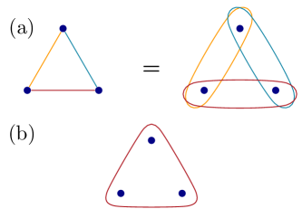
Figure 1: Examples of graphs and hypergraphs. Figure (a) shows a fully connected graph, which corresponds to the three-qubit GHZ state. In the hypergraph state formalism one often draws edges by circles (right) instead of lines as in the graph state formalism (left). The hypergraph state corresponding to the hypergraph in the lower figure (b) of the figure is local unitary equivalent to the state $\ket{H}=\left(\ket{000}+\ket{001}+\ket{010}+\ket{111}\right)/2$.

II Hypergraph States

In this section we present a short introduction to the class of hypergraph states and the description of transformations between them. Readers familiar with the topic may directly skip to the next section.

II.1 Definition of Hypergraph States

A hypergraph $H=(V,E)$ is a set $V$ of vertices and hyperedges $e\in E$ connecting them. Contrary to a normal graph, the edges in a hypergraph may connect more than two vertices; examples of hypergraphs are given in Figure 1.

Hypergraph states are multi-qubit quantum states, where the vertices and hyperedges of the hypergraph $H=(V,E)$ represent qubits and entangling gates, respectively. The state $\ket{H}$, corresponding to a hypergraph $H=(V,E)$ is defined as

$$\ket{H}=\prod_{e\in E}C_{e}\ket{+}^{\otimes\lvert V\rvert}\equiv U_{\text{ph}}\ket{+}^{\otimes\lvert V\rvert},$$ (1)

where $C_{e}$ is a generalized controlled-$Z$ gate, acting on qubits in the edge $e$ as $C_{e}=\operatorname{\mathds{1}}_{e}-2\outerproduct{11\ldots 1}{11\ldots 1}_{e}$. If an edge contains only a single vertex, $\lvert e\rvert=1$, then $C_{e}$ reduces to the Pauli-Z operator, and for two-vertex edges $C_{e}$ is just the standard two-qubit controlled phase gate. A detailed discussion on hypergraph state properties can be found in Refs. [25, 28].

Similarly as for graph states, there is an alternative definition using so-called stabilizing operators. First, one can define for each vertex $i$ a stabilizer operator,

$$S_{i}=U_{\text{ph}}X_{i}U_{\text{ph}}^{\dagger},$$ (2)

where $X_{i}$ denotes the first Pauli matrix acting on the $i$-th qubit and $U_{\text{ph}}$ denotes the collection of phase gates as in Eq. (1). Note that here only the gates with $i\in e$ matter. The stabilizing operators are non-local hermitian observables with eigenvalues $\pm 1$, they commute and generate an abelian group, the so-called stabilizer.

Then, a hypergraph state may be defined as a common eigenvector of all stabilizing operators $S_{i}$. Here, one has to fix the eigenvalues of the $S_{i}$. Often, the state defined in Equation 1 is called $\ket{H_{00\ldots 0}}$, as it is a common eigenstate of the $S_{i}$ with eigenvalue $+1$. By applying Pauli-Z gates on the state, one obtains states orthogonal to $\ket{H_{00\ldots 0}}$, where some of the eigenvalues are flipped to $-1.$ By applying all possible combinations of Z gates, one obtains a basis: $\{\ket{H_{\mathbf{k}}}=Z^{\mathbf{k}}\ket{H_{\mathbf{0}}}\}$, where $\mathbf{k}$ is a binary multi-index and $Z^{\mathbf{k}}=\bigotimes_{v\in V}Z^{k_{v}}_{v}$. In this notation, it holds that $S_{i}\ket{H_{\mathbf{k}}}=(-1)^{k_{i}}\ket{H_{\mathbf{k}}}$. Hence, $\ket{H_{\mathbf{k}}}$ is an eigenstate of $S_{i}$ with eigenvalue $(-1)^{k_{i}}$. It is convenient to write arbitrary states in the hypergraph basis:

$$\rho=\sum_{\mathbf{k},\mathbf{k^{\prime}}}c_{\mathbf{k},\mathbf{k^{\prime}}}\outerproduct{H_{\mathbf{k}}}{H_{\mathbf{k^{\prime}}}}.$$ (3)

Later we will purify states in this form to the state $\ket{H_{\mathbf{0}}}$.

II.2 Operations on Hypergraph States

Many operations on hypergraph states can be represented in a graphical manner. In the following we explain the effect of applying Pauli gates $X$ and $Z$, measuring in the corresponding basis $\sigma_{x}$ and $\sigma_{z}$, discuss how to represent the $\operatorname{\textsc{cnot}}$ gate graphically [29], and introduce the reduction operator $P_{v_{1},v_{2}}$ which we will need later. Note that in the following for Pauli matrices we use $X$ and $Z$ to denote the corresponding unitary transformation and $\sigma_{x}$ and $\sigma_{z}$ to denote the measurements. We only discuss transformations that are needed in the current paper, an overview on other transformations can be found in Ref. [28].

We have already mentioned the action of the unitary transformation $Z_{v}$ on some qubit $v$. It adds the edge $e=\{v\}$ to the set of edges $E$, if it was not contained before, or removes it otherwise. For example applying $Z_{2}$ and $Z_{3}$ to the left hypergraph state in Figure 2 would add a circle at vertex $2$ and remove the one at vertex $3$.

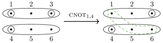
Figure 2: Example of a $\operatorname{\textsc{cnot}}_{1,4}$ gate (with control qubit 1 and target qubit 4) performed on a hypergraph state. Left: Hypergraph with vertex set $V=\{1,\dots,6\}$ and edge set $E=\{\{1\},\{1,2,3\},\{3\},\{4\},\{4,5,6\}\}$. Right: Hypergraph after applying $\operatorname{\textsc{cnot}}_{1,4}$. A new edge $\{1,5,6\}$ appeared while the edge $\{1\}$ vanished. The effect of applying the $\operatorname{\textsc{cnot}}_{1,4}$ gate is to introduce or delete edges from the set $E_{4}=\{\{1\},\{1,5,6\}\}$. The underlying rule is the following [29]: One takes the so-called adjacency $\operatorname{\mathcal{A}}(4)$ of the target qubit $t=4$, where one first considers all edges that contain $t$, but then removes $t$ from it. Here, we have $\operatorname{\mathcal{A}}(4)=\{\{\},\{5,6\}\}.$ Then, $E_{4}$ contains all edges which are unions of edges from $\operatorname{\mathcal{A}}(4)$ and the edge $\{1\}$ of the control qubit $c=1$.

The unitary transformation $X_{v}$ on a vertex $v$ of a hypergraph state $\ket{H}$ corresponding to the hypergraph $H=(V,E)$ is given by

$$X_{v}\ket{H}=\prod_{e\in E}C_{e}\prod_{e^{\prime}\in\operatorname{\mathcal{A}}(v)}C_{e^{\prime}}\ket{+}^{\otimes\lvert V\rvert},$$ (4)

where $\operatorname{\mathcal{A}}(v)$ is the adjacency of vertex $v$. This is a set of edges defined as

$$\operatorname{\mathcal{A}}(v)=\{e\setminus\{v\}\mid e\in E\text{ with }v\in e\}.$$ (5)

In words, to build the adjacency $\operatorname{\mathcal{A}}(v)$ one first takes the set of edges that contain $v$ and then removes $v$ from them. Examples of local transformations $X$ are given in Figure 3.

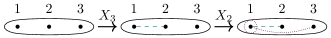
Figure 3: Application of $X$ operators on qubits 3 and 2. We first apply $X_{3}$ on the left graph. The adjacency of qubit 3 is given by $\operatorname{\mathcal{A}}(3)=\{\{1,2\}\}$. This new edge is shown by the blue dashed line in the middle graph. We then apply $X_{2}$ to the middle graph. The adjacency of qubit 2 is given by $\operatorname{\mathcal{A}}(2)=\{\{1\},\{1,3\}\}$. These new edges are shown by the dotted purple lines in the right graph.

Let us discuss now the graphical description of some local measurements on hypergraph states. In order to derive the post-measurement state after measuring vertex $v$, we can expand the state $\ket{H}$ at this vertex as

$$\ket{H}=\frac{1}{\sqrt{2}}\left(\ket{0}_{v}\ket{H_{0}}\pm\frac{1}{\sqrt{2}}\ket{1}_{v}\ket{H_{1}}\right),$$ (6)

where $\ket{H_{0}}$ and $\ket{H_{1}}$ are new hypergraph states with vertex set $V_{0}=V_{1}=V\setminus v$ and edge sets $E_{0}=\{e\in E\mid v\notin e\}$ and $E_{1}=E_{0}\cup\operatorname{\mathcal{A}}(v)$ [28]. After measuring $\sigma_{z}$, we therefore either get the state $\ket{H_{0}}$ or $\ket{H_{1}}$. Measuring $\sigma_{x}$ leads to a superposition of these two states and often the post-measurement state is then not a hypergraph sate anymore. In our case, we only measure $\sigma_{x}$ on qubits which are separated from other parts of the system. that is where $\ket{H_{0}}=\ket{H_{1}}$.

Applying a $\operatorname{\textsc{cnot}}_{ct}$ gate on a hypergraph state $H$, where $c$ is the control and $t$ the target, introduces or deletes hyperedges of the set $E_{t}=\{e_{t}\cup{c}\mid e_{t}\in\operatorname{\mathcal{A}}(t)\}$. The new edge set after applying $\operatorname{\textsc{cnot}}_{ct}$ is given by

$$E^{\prime}=E\triangle E_{t},$$ (7)

where $A\triangle B=A\cup B\setminus A\cap B$ is the symmetric difference of two sets. Since $C_{e}^{2}=\operatorname{\mathds{1}}$, double edges cancel out. Therefore, the operation $\operatorname{\textsc{cnot}}_{ct}$ deletes edges which are in $E$ and $E_{t}$ and introduces edges which are only in $E_{t}$. For example in the left part of Figure 2, the neighbourhood of vertex $4$ is given by $N(4)=\{\{\},\{5,6\}\}$ and therefore $E_{4}=\{\{1\},\{1,5,6\}\}$.

Finally, another operator which will be important later is the reduction operator $P_{v_{1},v_{2}}$, which maps two qubits to a single qubit. In the computational basis, the reduction operator is written as

$$P_{v_{1},v_{2}}=\outerproduct{0}{00}+\outerproduct{1}{11}.$$ (8)

It merges two vertices $v_{1},v_{2}$ to one which we call $v_{2}$. This action changes edges which contain $v_{1}$ into edges which contain $v_{2}$ and deletes edges $e,e^{\prime}$, with $e\neq e^{\prime}$ but $(e\setminus\{v_{1}\})=(e^{\prime}\setminus\{v_{2}\})$. The new edge set will therefore be

$$E^{\prime}=(\{e\in E|v_{1}\notin e\}\triangle\{f\cup\{v_{2}\}|f\in\operatorname{\mathcal{A}}(v_{1})\}).$$

An example is shown in Figure 4.

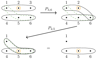
Figure 4: Application of the reduction projector $P_{3,6}$ and $P_{2,5}$. The projector merges two vertices and its corresponding edges to one. In the first step, we merge vertices 3 and 6. In the second step we merge vertices 2 and 5. This results in two times the same edge, the green dashed edge $\{1,5,6\}$ and the edge which was initially $\{1,2,3\}$ and such double edges cancel out.

III The CKDdV Purification Protocol

In this section we discuss the only known protocol which works for hypergraph states [27], we will refer to it as the CKDdV protocol. Originally, it was formulated for more general LME states. We first reformulate the purification protocol in a graphical manner, which makes it intuitively understandable. Based on this reformulation, we can then propose improvements.

In the simplest case, the aim is to purify a three-qubit state $\rho$ to a pure hypergraph state, chosen to be the state $\ket{H_{\mathbf{0}}}=C_{\{123\}}\ket{+}^{\otimes 3}$. The state is distributed between three parties, Alice, Bob, and Charlie. In the following, we explicitly describe the sub-protocol which reduces noise on Alice’s qubit. There are equivalent sub-protocols on Bob’s and Charlie’s qubits. The protocol is performed on two copies of a state $\rho$. Alice holds qubit $a_{1}$ of the first state and qubit $a_{2}$ of the second state, equivalently for Bob and Charlie.

The key idea of the protocol is to induce a transformation on the basis elements of the form

$$\ket{H_{i,j,k}}\ket{H_{i^{\prime},j^{\prime},k^{\prime}}}\rightarrow\delta_{i,i^{\prime}}\ket{H_{i,j+j^{\prime},k+k^{\prime}}},$$ (9)

where $\delta_{i,i^{\prime}}$ denotes the Kronecker delta. This means that the sub-protocol compares the indices $i,i^{\prime}$ on Alice’s qubits, and the state is discarded when $i\neq i^{\prime}$. This map drives a general state as in Eq. (3) closer to the desired hypergraph state. In detail, the sub-protocol which implements this transition is given by:

Protocol 1 (CKDdV protocol).

(0) Alice, Bob, and Charlie share two copies of a state.

(i) Alice applies a local $\operatorname{\textsc{cnot}}_{a_{1},a_{2}}$ gate on her qubits.

(ii) Bob and Charlie apply local reduction operators $P_{v_{1},v_{2}}$ on their qubits.

(iii) Alice measures qubits $a_{1}$ in the $\sigma_{x}$ basis. She keeps the state, if the outcome is “$+1$”, and discards it otherwise.

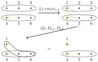
Figure 5: The CKDdV protocol, as described in in 1. In the figure, the transformation of the two basis elements $\ket{H_{000}}\ket{H_{100}}$ is shown. In step (i), Alice performs a local $\operatorname{\textsc{cnot}}_{1,4}$ gate. Then, Bob and Charlie apply local reduction operators $P_{2,5}$ and $P_{3,6}$, respectively. Double edges cancel out, so that the green dashed line and the former edge $\{1,2,3\}$ vanish. In step (iii), Alice measures qubit 1 in the $\sigma_{x}$ basis. If there is a single-qubit edge on vertex 1, as the orange one in this figure, her measurement outcome will be “$-1$” and therefore the state gets discarded. If one ignores all orange single-qubit edges in the figure, this corresponds to the transformation of the basis elements $\ket{H_{000}}\ket{H_{000}}$. In this case, Alice’s measurement outcome will be “$+1$” and the remaining state $\ket{H_{000}}$ is kept.

In Figure 5 it is shown how the basis elements $\ket{H_{000}}\ket{H_{i00}}$ transform.

In order to purify the full state, one needs to choose a sequence of sub-protocols in which these sub-protocols are applied on different parties. In Ref. [27], the sequence ABC-CAB-BCA was favoured, as it seems to perform better than just repeating the sequence ABC. The reason is that the qubit of Charlie becomes more noisy due to the back action from the sub-protocols purifying Alice’s and Bob’s qubits.

IV Improving the Protocol Performance

In order to purify towards one state of a certain fidelity, one needs a number of input states, which depends exponentially on the number of iterations, as in each run of the protocol a certain fraction of states is discarded. Therefore it is of high interest to apply the subprotocols in a sequence which works as efficient as possible. As already pointed out by Carle et al. [27], it depends on the input state which sequence is the most advantageous and it is not trivial to see which sequence is optimal. Carle et al. decided to use the sequence $S={\rm ABC-CAB-BCA}$ in all their applications, since it performs well in many cases. In the following we will ask whether the proposed sequence really is the best and how we can potentially find better sequences.

One should notice that in step (ii) of the protocol a large fraction of states is discarded. The operator $P_{v_{1},v_{2}}$ corresponds to a positive map, which maps two qubits, which are in the same state, to one qubit and both qubits are discarded, if they are in different states. This can be seen as one outcome of a measurement. In the second part of this section we will ask whether one can reduce the amount of discarded states.

IV.1 Improved and Adaptive Sequences

Consider a noisy three-qubit state $\rho(p)$, where $p$ is a noise parameter for some noise model, which should be purified to the pure hypergraph state $\outerproduct{H_{000}}{H_{000}}$. Clearly, for a fixed sequence $S$ there is a maximal amount of noise until which the state can still be purified and there is a regime, where one cannot purify it any more.

Interestingly, for some parameter regimes where the state cannot be purified, the purification protocol does not converge towards a state with random noise, but towards a specific state which is a mixture of two states: either $\frac{1}{2}(\outerproduct{H_{000}}{H_{000}}+\outerproduct{H_{001}}{H_{001}})$, $\frac{1}{2}(\outerproduct{H_{000}}{H_{000}}+\outerproduct{H_{010}}{H_{010}})$, or $\frac{1}{2}(\outerproduct{H_{000}}{H_{000}}+\outerproduct{H_{100}}{H_{100}})$. This observation gives insights about how good the purification works on different parties. The protocol eliminates noise on two parties but fails on the third party. For example if we apply sequence $S={\rm ABC}$, in the cases we tested, there is a regime, where the state does not get purified but converges to $\frac{1}{2}(\outerproduct{H_{000}}{H_{000}}+\outerproduct{H_{001}}{H_{001}})$.

This is consistent with the explanation given in Ref. [27] that the purification has an disadvantage on Charlie’s site. It may be explained as follows: By performing the protocol at one party, one aims to reduce noise on this party. As an unwanted side effect, one increases noise on the other parties. This happens because if there is noise on the first input state, the local reduction operator will “copy” it to the second state (see Equation 9). So, when choosing sequence $S={\rm ABC}$, one increases the noise on Charlie’s qubit two times before purifying it the first time.

How well the protocol performs on each party can be analysed using the measurement statistics obtained in step (iii) of the protocol. The probability to measure outcome “$+1$” in step (iii) on a qubit belonging to a certain party gives insights, how much noise the state on this party has. On the perfect target state, one does not detect any noise and therefore measures outcome “$+1$” with probability equal to one. If one applies the protocol to the state $\frac{1}{2}(\outerproduct{H_{000}}{H_{000}}+\outerproduct{H_{001}}{H_{001}})$, however, one obtains outcome “$+1$” with a probability equal to one or 0.5, depending on which subprotocol was applied. If it was the subprotocol where Alice’s or Bob’s qubits are measured in step (iii), the probability is equal to one. If it was the subprotocol where Charlie’s qubit was measured the probability is 0.5. So, by evaluating the probabilities to measure outcome “$+1$” in step (iii) of the protocol, one can analyse the efficiency of the sequence.

All in all, we use two approaches to find better sequences. The first approach is to find an optimal sequence, which allows a high noise tolerance and will be applied later without further observation of the statistics. The second approach uses two sequences where we switch from one to the other depending on the measurement outcomes during the process. The first approach helps to find sequences which are more efficient also for purification of states with a low noise level. The second approach gives a method to purify states which would not be purifyable otherwise.

We assume that we know how often we want to apply the protocol and therefore how many copies of the initial state are needed. We perform the first subprotocol on all copies and get a certain fraction of output states. We then perform the second subprotocol on all output states and so on. With this procedure, we do multiple measurements on copies of states such that we can approximate a probability from the frequency of a certain outcome. We further assume that we repeat this procedure several times, that is, we produce a certain number of copies of input states, purify them and start again from the beginning. In each run, we can vary the sequence, using what we have learned in the run before. We restricted ourselves to sequences of length nine. The best sequence we find in this way we call $S_{1}$.

It is not known how the efficiency of the sequence depends on the state. Therefore, even if the state is known, one needs to sample which sequence works best. However, there are some observations which can be used to find better sequences. We notice that it is reasonable to consider permutations of A, B, C together. We further notice, that the first party of the triple experiences the largest impact. It is also a good strategy to address the same party in two consecutive rounds, that is on the last position of one triple and on the first position of the following triple. The sequence proposed by Carle et al. fulfills all mentioned properties and is in principle a good starting sequence. After gaining experience how efficient the sequence works for the given state, one can exchange few positions and evaluate its impact. We will see later (i.e. in Tables 1 and 4) that the optimal sequences $S_{1}$ we found for different states, support our observations. Every triple is a permutation of A,B,C. We see that except of one case, the first position of one triple is equal to either the first or the last position of the previous triple. However, it consumes many states to find good sequences. Another strategy could be to estimate the corresponding density matrix of the given state by local tomography and find the optimal sequence by simulations on the computer.

With the second approach, we give a way to purify states which can not be purified by sequence $S_{1}$ because their initial fidelity is slightly beyond the threshold. We start using sequence $S_{1}$ and switch to sequence $S_{2}$ depending on the measurement outcomes of step (iii). Our switching condition is the following: After each measurement of step (iii), we evaluate the probability to measure “$-1$” for the given party. Based on the last three probabilities associated to the same party, we take a decision to switch or not. For $\vec{x}$ being the vector of this three probabilities, where $x_{3}$ is the newest probability, we switch, if the product of the vectors $\vec{a}\vec{x}$ exceed a bound $b$ where $\vec{a}$ is a weight vector. In real applications we can not evaluate the probability. We suggest to count appearance of certain outcomes and estimate the probability from the frequency.

	$\operatorname{\mathcal{E}}_{\text{wn}}(\rho,p)$	$\operatorname{\mathcal{E}}_{\text{deph}}(\rho,p)$	$\operatorname{\mathcal{E}}_{\text{depo}}(\rho,p)$
$S_{1}$	ABC-CBA-ABC	ABC-CBA-CBA	ABC-CAB-BCA
$S_{2}$	BAB-CAB-ABA	CCC-ACB-CBC	BBB-BCB-BBB-BAB
$\vec{a}$	$(0.33,0.35,0.32)$	$(0.35,0.43,0.21)$	$(0.35,0.34,0.31)$
$b$	0.35	0.39	0.44

Table 1: Sequences $S_{1}$, $S_{2}$, approximate weight vectors $\vec{a}$, and bounds $b$ for states with three kinds of noise. Explanation see text.

To see the efficiency of our methods, we consider different noise models. We analyze the influence of global white noise described by the channel

$$\operatorname{\mathcal{E}}_{\text{wn}}(\rho,p)=p\rho+\frac{1-p}{2^{n}}\operatorname{\mathds{1}},$$ (10)

where $n$ is the number of qubits. In this section, the number of states is $n=3$. We further analyse local noise channels given by $\operatorname{\mathcal{E}}(\rho,p)=\bigotimes_{i=1}^{n}\operatorname{\mathcal{E}}^{i}(\rho,p)$, where $\operatorname{\mathcal{E}}^{i}$ is either the dephasing channel

$$\operatorname{\mathcal{E}}_{\text{deph}}^{i}(\rho,p)=p\rho+\frac{1-p}{2}(\rho+Z_{i}\rho Z_{i})$$ (11)

or the depolarizing channel

$$\operatorname{\mathcal{E}}_{\text{depo}}^{i}(\rho,p)=p\rho+\frac{1-p}{4}(\rho+X_{i}\rho X_{i}+Y_{i}\rho Y_{i}+Z_{i}\rho Z_{i}).$$ (12)

The sequences, weight vectors and bounds we found to be optimal are given in Table 1. To compare the approaches, we give the noise thresholds found in Ref. [27], obtained by our sequence $S_{1}$, and by the adaptive approach in Table 2. The sequences we found are also better in other perspectives. If we apply the new sequences $S_{1}$ nine rounds on given input states, we see that the output states have a higher fidelity then after purifying the same state nine rounds using the sequence given in Ref. [27].

	$p_{\text{min}}$ from [27]	$p_{\text{min}}$ from $S_{1}$	$p_{\text{min}}$ from
			adaptive protocol
$\operatorname{\mathcal{E}}_{\text{wn}}(\rho,p)$	0.6007	0.5878	0.5876
$\operatorname{\mathcal{E}}_{\text{deph}}(\rho,p)$	0.8013	0.7803	0.7747
$\operatorname{\mathcal{E}}_{\text{depo}}(\rho,p)$	0.8136	0.8136	0.8132

Table 2: Noise thresholds $p_{\text{min}}$ reproduced from Ref. [27], gained from our sequences $S_{1}$ (see Table 1), and for the adaptive approach. In the case of $\operatorname{\mathcal{E}}_{\text{depo}}(\rho,p)$ we found that the sequence from Ref. [27] was already the best sequence of length 9. Therefore there is no improvement of $p_{\text{min}}$ in this case.

IV.2 Recycling of Discarded States

If one wishes to purify a state using the CKDdV protocol one needs a high number of input states in order to obtain one state of a certain fidelity. Let us count how many states we need to have one state after applying the protocol once. In step (0) of the protocol, one takes two input states. One does not loose states by applying $\operatorname{\textsc{cnot}}$ in step (i). By applying the reduction operator $P_{v_{1},v_{2}}$, approximately $\frac{1}{2}$ of the pairs are lost. Since this operator is applied on two parties in step (ii), one needs approximately four pairs. In step (iii), one measures outcome “$+1$” with a probability $\leqslant 1$. This probability depends on the fidelity of the states and increases with increasing fidelity. So, in total, approximately $8$ input states are required to obtain one output state. To prepare a state for which we need to apply the protocol $m$ times, we need more than $8^{m}$ input stats. To purify, for example, a state of initial fidelity 0.93 to a state of fidelity of 0.994, we need three steps. The required number of input states to obtain one output state is roughly $8.7^{3}\approx 660$. If we want to purify the same state to a fidelity of $0.999$, which we reach after six steps, we need about $8.38^{6}\approx 346\ 000$ input states to get one new state.

It is natural to try to use the available quantum states more efficiently. In step (ii) of the CKDdV protocol, one performs a projective measurement and considers only one outcome, namely $P_{v_{1},v_{2}}$, which we get with probability approximately $\frac{1}{2}$. We suggest to use the states which were discarded because we measured something different than $P_{v_{1},v_{2}}$. The second reduction operator $P_{v_{1},v_{2}}^{\perp}$ is perpendicular to $P_{v_{1},v_{2}}$ and defined as

$$P_{v_{1},v_{2}}^{\perp}=\outerproduct{0}{10}+\outerproduct{1}{01}=P_{v_{1},v_{2}}(X_{v_{1}}\otimes\operatorname{\mathds{1}}_{v_{2}}).$$ (13)

As $P_{v_{1},v_{2}}$, the operator $P_{v_{1},v_{2}}^{\perp}$ is a positive map. It maps two qubits, which are in different states, to one qubit. This can be seen as a different measurement outcome than $P_{v_{1},v_{2}}$, or one may interpret the set $\{P_{v_{1},v_{2}},P_{v_{1},v_{2}}^{\perp}\}$ as a quantum instrument.

In the original CKDdV protocol one keeps the state only after measuring $P_{b_{1},b_{2}}P_{c_{1},c_{2}}$. There are three more possible measurement outcomes: $P_{b_{1},b_{2}}P_{c_{1},c_{2}}^{\perp}$, $P_{b_{1},b_{2}}^{\perp}P_{c_{1},c_{2}}$, and $P_{b_{1},b_{2}}^{\perp}P_{c_{1},c_{2}}^{\perp}$. In the cases of measuring $P_{v_{1},v_{2}}^{\perp}$ on at least one party, one obtains a post measurement state on which one can apply some corrections to get a state, which is similar to the input state. One can collect these states and further purify them.

So, one can write down a modified protocol of the CKDdV protocol. Here, we give the sub-protocol which reduces noise on Alice’s qubits. The sub-protocols for Bob and Charlie work equivalently.

Protocol 2 (Improved CKDdV protocol).

(0) Alice, Bob, and Charlie share two copies of a state.

(i) Alice applies a local $\operatorname{\textsc{cnot}}_{a_{1},a_{2}}$ gate on her qubits.

(ii) Bob and Charlie perform a measurement on their qubits and measure the local reduction operators $P_{v_{1},v_{2}}$ and $P_{v_{1},v_{2}}^{\perp}$. If the measurement outcome for Bob and Charlie was $P_{v_{1},v_{2}}$, continue with step (iiia). Else, continue with (iiib)

(iiia) After Bob and Charlie both measured $P_{v_{1},v_{2}}$, Alice measures qubits $a_{1}$ in the $\sigma_{x}$ basis. She keeps the state, if the outcome is “$+1$”, and discards it otherwise.

(iiib) After measuring $P_{v_{1},v_{2}}^{\perp}$ on at least one pair of Bob and Charlie’s qubits, Alice measures her qubit $a_{1}$ in the $\sigma_{z}$ basis. If she measure “$+1$”, she keeps the state as it is. Otherwise, Bob and Charlie apply some local unitaries, which depend on the combinations of measurement outcomes in step (ii) and are given in Table 3.

Measurement	local correction	local correction
outcomes	Bob	Charlie
$P_{b_{1},b_{2}}P_{c_{1},c_{2}}^{\perp}$	$Z$	$\operatorname{\mathds{1}}$
$P_{b_{1},b_{2}}^{\perp}P_{c_{1},c_{2}}$	$\operatorname{\mathds{1}}$	$Z$
$P_{b_{1},b_{2}}^{\perp}P_{c_{1},c_{2}}^{\perp}$	$Z$	$Z$

Table 3: In 2 step (iiib), Alice measures her qubit $a_{1}$ in the $Z$ basis. If her outcome is “$-1$”, Bob and Charlie have to apply local corrections to their qubits. The local corrections depend on their measurement outcomes from step (ii) and are given in this table. The first case is shown in Figure 6.

The key idea is that output states from step (iiib) can be collected and further purified. In case of measuring $P_{v_{1},v_{2}}^{\perp}$ on at least one party, the protocol gives us a transition

$$\ket{H_{i,j,k}}\ket{H_{i^{\prime},j^{\prime},k^{\prime}}}\rightarrow\ket{H_{i^{\prime},j+j^{\prime},k+k^{\prime}}}.$$ (14)

The resulting state has in general a lower fidelity than the input state. This is caused by the same reason of “copying” noise, as discussed before. Since in the considered case the protocol does not reduce noise, the fidelity drops.

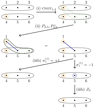
Figure 6: Modified 2 for the same initial states as shown in Figure 5 for the case to measure $P_{b_{1},b_{2}}P_{c_{1},c_{2}}^{\perp}$ in step (ii). Alice performs a $\sigma_{z}^{(1)}$-measurement on her qubit 1 of the state in the second raw. If she gets outcome “$+1$” in step (iiib), the resulting state is the same as the initial state (qubits 4, 5 and 6). If she gets outcome “$-1$”, Bob’s qubit 5 has a decoration, which he needs to correct. After Bob applied a local $Z_{5}$ unitary on qubit 5, again the resulting state is the same as the initial state (qubits 4, 5 and 6). Note that this is only the case, if there is no noise on qubit 2 and 3, as shown in this figure. In general one obtains the state given in Equation 14.

An example for 2 is shown in Figure 6, where we assume the case that Bob measures $P_{2,5}$ and Charlie measures $P_{3,6}^{\perp}$. In this case, the local correction after measuring outcome “$-1$” is applying a unitary $Z_{5}$ at qubit 5.

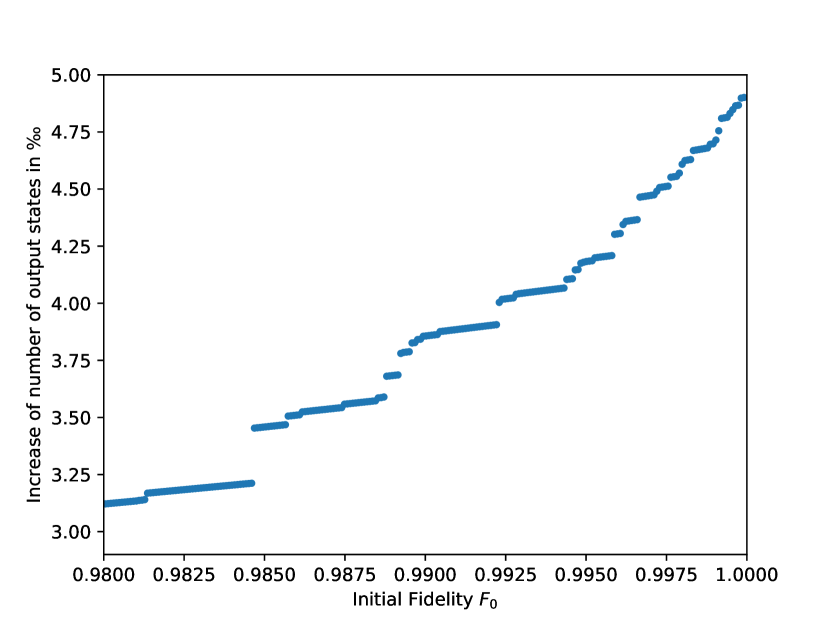
Figure 7: Effect of using 2 instead of the original CKDdV protocol. The input states are given by $\operatorname{\mathcal{E}}_{\text{wn}}(\outerproduct{H_{\mathbf{0}}}{H_{\mathbf{0}}},p)$. We first apply 1 three times and computed the fidelity $F_{3}$ of the output states. Then, we apply 2 on the same input states and compare how many more output states of fidelity $\geqslant F_{3}$ we get. The figure displays the increase of output states by using 2, depending on the fidelity $F_{0}$ of the input states.

Given a certain number of input states which we want to purify to a target fidelity, we obtain more output states of the desired fidelity if we follow 2 instead of the original CKDdV protocol. The effect in the cases we tested turned out, however, to be small. As input states, we chose the state $\outerproduct{H_{000}}{H_{000}}$ mixed with white noise. We first applied 1 three times, that is, once on each party, and computed the fidelity $F_{3}$ of the output states. Then, we applied 2 on the same input states and compared how many more output states of fidelity $\geqslant F_{3}$ we get. In Figure 7 we show how much the number of output states increase by using 2, depending on the fidelity $F_{0}$ of the input states. In the chosen cases, we get approximately 0.4 % more output states from using 2 instead of the CKDdV protocol.

A similar idea of reusing states which get discarded in most protocols was proposed in Ref. [26]. Zhou et al. consider Bell states and reuse states from the last step of the protocol, which is equivalent to step (iii) in the CKDdV protocol.

V Generalisation to More Qubits

The methods described here can also be applied to states with more qubits and different arrangement of edges. We restrict our attention to hypergraphs which are $k$-regular and $k$-colorable. A hypergraph is $k$-regular, if all edges $e\in E$ have order $k$ and it is $k$-colorable, if it is possible to color vertices of a hypergraph using $k$ colors such that no two vertices of the same color share a common edge. For example, the hypergraph states shown in Figures 2 and 8 are 3-colorable and 3-regular. In this section we discuss purification protocols to hypergraph states of more than 3 qubits which are 3-colorable and 3-regular. In the following, we will denote the colors by $A$, $B$, and $C$.

The protocols can be generalised by letting all parties holding qubits of color $A$ do what was described for Alice before. In the same way, parties holding a qubit of color $B$ or $C$ do what was described for Bob or Charlie, respectively. For a explicit formulation of the generalized protocol, see Ref. [27].

	$p_{\text{min}}$ from	$p_{\text{min}}$	sequence $S_{1}$
	$S_{\text{CKDdV}}$	from $S_{1}$
$\operatorname{\mathcal{E}}_{\text{wn}}(\rho_{3},p)$	0.6007	0.5878	ABC-CBA-ABC
$\operatorname{\mathcal{E}}_{\text{wn}}(\rho_{4},p)$	0.4633	0.4396	ABC-ACB-BCA
$\operatorname{\mathcal{E}}_{\text{wn}}(\rho_{5},p)$	0.3901	0.3486	ABC-ABC-CBA
$\operatorname{\mathcal{E}}_{\text{wn}}(\rho_{6},p)$	0.3341	0.3017	ABC-ACB-BAC*
$\operatorname{\mathcal{E}}_{\text{deph}}(\rho_{3},p)$	0.8013	0.7803	ABC-CBA-CBA
$\operatorname{\mathcal{E}}_{\text{deph}}(\rho_{4},p)$	0.8014	0.7803	ABC-CBA-CBA*
$\operatorname{\mathcal{E}}_{\text{deph}}(\rho_{5},p)$	0.8014	0.7803	ABC-CBA-CBA*
$\operatorname{\mathcal{E}}_{\text{deph}}(\rho_{6},p)$	0.8014	0.7803	ABC-CBA-CBA*
$\operatorname{\mathcal{E}}_{\text{depo}}(\rho_{3},p)$	0.8137	0.8136	ABC-CAB-BCA
$\operatorname{\mathcal{E}}_{\text{depo}}(\rho_{4},p)$	0.8306	0.8122	BAC-CBA-CAB
$\operatorname{\mathcal{E}}_{\text{depo}}(\rho_{5},p)$	0.8358	0.8128	ACB-BCA-CBA
$\operatorname{\mathcal{E}}_{\text{depo}}(\rho_{6},p)$	0.8144	0.8121	ABC-CBA-CAB

Table 4: Noise thresholds $p_{\text{min}}$ for the sequence $S_{\text{CKDdV}}$ proposed in Ref. [27] and new sequences $S_{1}$. The index of the state gives the number of qubits. In the case of $\operatorname{\mathcal{E}}_{\text{depo}}(\rho_{3},p)$ we found that the sequence from Ref. [27] was already the best sequence of length 9. Therefore there is no improvement of $p_{\text{min}}$. When we found (non-trivially) different sequences of the same length, we marked them with an asterisk.

We analysed linear three-colorable states with up to six qubits under the influence of global white noise, dephasing and depolarisation. That is the states to which we want to purify are $U_{123}U_{234}\ket{+}^{\otimes 4}$, $U_{123}U_{234}U_{345}\ket{+}^{\otimes 5}$, and $U_{123}U_{234}U_{345}U_{456}\ket{+}^{\otimes 6}$, as shown in Figure 8. We compare the noise threshold $p_{\text{min}}$ for the sequence proposed in Ref. [27] with new sequences $S_{1}$, found using methods described in Section IV.1.

Our results are shown in Table 4. One sees that in the case of white noise for more qubits, the differences in the noise threshold $p_{\text{min}}$ become more significant. Therefore, especially in these cases it is more relevant to find good sequences. For the tested states with dephasing and depolarisation noise, the noise threshold is constant or varies slightly, respectively.

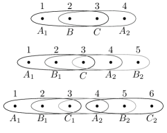
Figure 8: Linear 3-colorable and 3-regular hypergraph states with 4, 5, and 6 qubits. The colors are denoted by $A$, $B$, and $C$. Note that two qubits which have the same color, for example qubits 1 and 4, still belong to different parties. Since we are restricted to local operations, we can only perform operations on qubits of the same party, that is in general not on qubits of the same color.

VI Conclusion and Outlook

In this paper we discussed protocols for entanglement purification of hypergraph states. First, we reformulated the CKDdV protocol in a graphical language. This offers a new way to understand the protocol, furthermore, it allows to search for systematic extensions. Consequently, we introduced several improvements of the original protocol. These improvements are based on different sequences, adaptive schemes, as well as methods to recycle some of the unused states. While these modifications are conceptually interesting and can indeed improve the performance in various examples, the amount of the improvement in realistic examples seems rather modest.

The problem of finding efficient sequences is also relevant for purification protocols for other states and was raised for example in Ref.  [4] in the context of two-colorable graph states. The methods developed here can be applied to this case, but also to all purification protocols which follow the concept introduced by Bennett et al.  [1].

A further open question is how the effects of our methods scale with the number of qubits. Another open question is whether 2 can be further improved so that the effect gets more significant.

VII Acknowledgments

We thank Mariami Gachechiladze, Kiara Hansenne, Jan L. Bönsel, Fabian Zickgraf, Yu-Bo Sheng, Lucas Tendick, and Owidiusz Makuta for discussions. This work was supported by the Deutsche Forschungsgemeinschaft (DFG, German Research Foundation, project numbers 447948357 and 440958198), the Sino-German Center for Research Promotion (Project M-0294), the ERC (Consolidator Grant 683107/TempoQ), the German Ministry of Education and Research (Project QuKuK, BMBF Grant No. 16KIS1618K), and the Stiftung der Deutschen Wirtschaft.

References

- Bennett et al. [1996a] C. H. Bennett, H. J. Bernstein, S. Popescu, and B. Schumacher, Phys. Rev. A 53, 2046 (1996a).
- Bennett et al. [1996b] C. H. Bennett, D. P. DiVincenzo, J. A. Smolin, and W. K. Wootters, Phys. Rev. A 54, 3824 (1996b).
- Deutsch et al. [1996] D. Deutsch, A. Ekert, R. Jozsa, C. Macchiavello, S. Popescu, and A. Sanpera, Phys. Rev. Lett. 77, 2818 (1996).
- Aschauer et al. [2005] H. Aschauer, W. Dür, and H.-J. Briegel, Phys. Rev. A 71, 012319 (2005).
- Kruszynska et al. [2006] C. Kruszynska, A. Miyake, H. J. Briegel, and W. Dür, Phys. Rev. A 74, 052316 (2006).
- Miyake and Briegel [2005] A. Miyake and H. J. Briegel, Phys. Rev. Lett. 95, 220501 (2005).
- Dür and Briegel [2007] W. Dür and H. J. Briegel, Rep. Prog. Phys. 70, 1381 (2007).
- Kwiat et al. [2001] P. G. Kwiat, S. Barraza-Lopez, A. Stefanov, and N. Gisin, Nature 409, 1014 (2001).
- Pan et al. [2003] J.-W. Pan, S. Gasparoni, R. Ursin, G. Weihs, and A. Zeilinger, Nature 423, 417 (2003).
- Hu et al. [2021] X.-M. Hu, C.-X. Huang, Y.-B. Sheng, L. Zhou, B.-H. Liu, Y. Guo, C. Zhang, W.-B. Xing, Y.-F. Huang, C.-F. Li, and G.-C. Guo, Phys. Rev. Lett. 126, 010503 (2021).
- Huang et al. [2022] C.-X. Huang, X.-M. Hu, B.-H. Liu, L. Zhou, Y.-B. Sheng, C.-F. Li, and G.-C. Guo, Sci. Bull. 67, 593 (2022).
- Hein et al. [2004] M. Hein, J. Eisert, and H. J. Briegel, Phys. Rev. A 69, 062311 (2004).
- Kruszynska and Kraus [2009] C. Kruszynska and B. Kraus, Phys. Rev. A 79, 052304 (2009).
- Qu et al. [2013] R. Qu, J. Wang, Z.-s. Li, and Y.-r. Bao, Phys. Rev. A 87, 022311 (2013).
- Rossi et al. [2013] M. Rossi, M. Huber, D. Bruß, and C. Macchiavello, New J. Phys. 15, 113022 (2013).
- Shor [1995] P. W. Shor, Phys. Rev. A 52, R2493 (1995).
- Wagner et al. [2018] T. Wagner, H. Kampermann, and D. Bruß, J. Phys. A Math. Theor. 51, 125302 (2018).
- Raussendorf and Briegel [2001] R. Raussendorf and H. J. Briegel, Phys. Rev. Lett. 86, 5188 (2001).
- Gachechiladze et al. [2019] M. Gachechiladze, O. Gühne, and A. Miyake, Phys. Rev. A 99, 052304 (2019).
- Scarani et al. [2005] V. Scarani, A. Ací n, E. Schenck, and M. Aspelmeyer, Phys. Rev. A 71, 042325 (2005).
- Gühne et al. [2005] O. Gühne, G. Tóth, P. Hyllus, and H. J. Briegel, Phys. Rev. Lett. 95, 120405 (2005).
- Gachechiladze et al. [2016] M. Gachechiladze, C. Budroni, and O. Gühne, Phys. Rev. Lett. 116, 070401 (2016).
- Morimae et al. [2017] T. Morimae, Y. Takeuchi, and M. Hayashi, Phys. Rev. A 96, 062321 (2017).
- Baccari et al. [2020] F. Baccari, R. Augusiak, I. Šupić, J. Tura, and A. Acín, Phys. Rev. Lett. 124, 020402 (2020).
- Gühne et al. [2014] O. Gühne, M. Cuquet, F. E. S. Steinhoff, T. Moroder, M. Rossi, D. Bruß, B. Kraus, and C. Macchiavello, J. Phys. A Math. Theor. 47, 335303 (2014).
- Zhou et al. [2020] L. Zhou, W. Zhong, and Y.-B. Sheng, Opt. Express 28, 2291 (2020).
- Carle et al. [2013] T. Carle, B. Kraus, W. Dür, and J. I. de Vicente, Phys. Rev. A 87, 012328 (2013).
- Gachechiladze [2019] M. Gachechiladze, Quantum hypergraph states and the theory of multiparticle entanglement, Ph.D. thesis, Universität Siegen (2019).
- Gachechiladze et al. [2017] M. Gachechiladze, N. Tsimakuridze, and O. Gühne, J. Phys. A Math. Theor. 50, 19LT01 (2017).