SemSup-XC: Semantic Supervision for Extreme Classification

Abstract

Extreme classification (XC) involves predicting over large numbers of classes (thousands to millions), with real-world applications like news article classification and e-commerce product tagging. The zero-shot version of this task requires generalization to novel classes without additional supervision. In this paper, we develop SemSup-XC, a model that achieves state-of-the-art zero-shot and few-shot performance on three XC datasets derived from legal, e-commerce, and Wikipedia data. To develop SemSup-XC, we use automatically collected semantic class descriptions to represent classes and facilitate generalization through a novel hybrid matching module that matches input instances to class descriptions using a combination of semantic and lexical similarity. Trained with contrastive learning, SemSup-XC significantly outperforms baselines and establishes state-of-the-art performance on all three datasets considered, gaining up to 12 precision points on zero-shot and more than 10 precision points on one-shot tests, with similar gains for recall@10. Our ablation studies highlight the relative importance of our hybrid matching module and automatically collected class descriptions.

1 Introduction

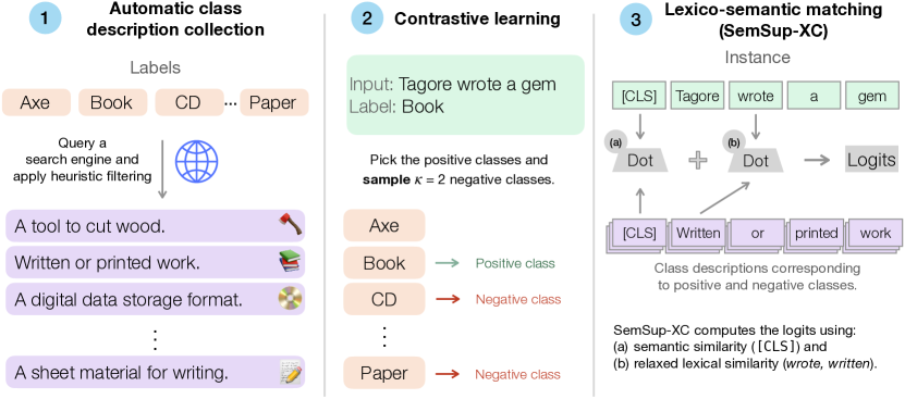
Figure 1: Our model SemSup-XC achieves state-of-the-art performance on zero-shot and few-shot extreme classification through three innovations – [baseline=(char.base)] [shape=circle, fill=approach, draw=approach, text=black, inner sep=1.2pt, scale=0.9, font=] (char) 1; large-scale automated class description collection with heuristic filtering to improve semantic understanding of classes, [baseline=(char.base)] [shape=circle, fill=approach, draw=approach, text=black, inner sep=1.2pt, scale=0.9, font=] (char) 2; contrastive learning to make training faster by over 99% when compared to the previous work (semsup), and [baseline=(char.base)] [shape=circle, fill=approach, draw=approach, text=black, inner sep=1.2pt, scale=0.9, font=] (char) 3; a novel lexico-semantic matching model building called Hybrid-Match to utilize both semantic similarity at the sentence level and contextual lexico-semantic similarity at the token level.

Extreme classification (XC) studies the problem of predicting over a large space of classes, ranging from thousands to millions (Agrawal2013MultilabelLW; bengio2019extreme; Bhatia2015SparseLE; Chang2019AMD; Lin2014MultilabelCV; Jiang2021LightXMLTW). This paradigm has multiple real-world applications including movie and product recommendation, search-engines, and e-commerce product tagging. In many of these applications, models are required to handle the addition of new classes on a regular basis, which has been the subject of recent work on zero-shot and few-shot extreme classification (ZS-XC and FS-XC) Gupta2021GeneralizedZE; Xiong2022ExtremeZL; Simig2022OpenVE. These setups are challenging because of (1) the presence of a large number of fine-grained classes which are often not mutually exclusive, (2) limited or no labeled data per class, and (3) increased computational expense and model size due to the large label space. While the aforementioned works have tried to tackle the latter two issues, they lack a semantically rich representation of classes, and instead rely on class names or hierarchies to represent them.

In this work, we leverage semantic supervision (semsup) (Hanjie2022SemanticSE) for developing models for extreme classification. SemSup-XC represents classes using multiple diverse class descriptions, which allows it to generalize naturally to novel classes when provided with corresponding descriptions. However, semsup as proposed in Hanjie2022SemanticSE cannot be naively applied to XC for several reasons: (1) semsup requires encoding descriptions of all classes for each training batch, which is prohibitively computationally expensive for large label spaces, (2) it uses semantic similarity only at the sentence level between the instance and label description, and (3) it requires human intervention to collect descriptions, which is expensive for extremely large label spaces we are dealing with.

We remedy these deficiencies by developing SemSup-XC, a model that scales to large class spaces in XC and establishes a new state-of-the-art using three innovations. First, we use a novel hybrid lexical-semantic similarity model (Hybrid-Match) that combines semantic similarity of sentences with relaxed lexical-matching between all token pairs. Second, we propose semsup-web – an automatic pipeline with precise heuristics to discover high-quality descriptions. Finally, we use a contrastive learning objective that samples a fixed number of negative label descriptions, improving computation speed by up to 99% when compared to semsup.

SemSup-XC achieves state-of-the-art performance on three diverse XC datasets from legal (EURLex), e-commerce (AmazonCat), and wiki (Wikipedia) domains, across zero-shot (ZS-XC), generalized zero-shot (GZS-XC) and few-shot (FS-XC) settings. For example, on ZS-XC, SemSup-XC outperforms the next best baseline by $5-12$ precision points over all datasets and all metrics. On FS-XC, SemSup-XC consistently outperforms baselines by over $10$ P@1 points on the EURLex and AmazonCat datasets. Surprisingly, SemSup-XC even outperforms larger unsupervised language models like T5 and Sentence Transformers (e.g., by over $30$ P@1 points on EURLex) which are pre-trained on much larger web-scale corpora. Our ablation studies dissect the importance of each component in SemSup-XC, and shows the importance of our proposed hybrid matching module. Qualitative error analysis of our model (Table 6) shows that it predicts diverse correct classes that are applicable to the instance at times, whereas other models either predict incorrect classes or suffer a mode collapse.

2 Methodology

2.1 Background

Extreme Classification

Extreme classification deals with prediction over large label spaces (thousands to millions classes) and multiple correct classes per instance (multi-label) Agrawal2013MultilabelLW; Bhatia2015SparseLE; Babbar2017DiSMECDS; Gupta2021GeneralizedZE; Xiong2022ExtremeZL; Simig2022OpenVE. Zero-shot extreme classification (ZS-XC) is a variant where models are evaluated on unseen classes not encountered during training. We evaluate both on (1) zero-shot (ZS), where the model is tested only on unseen classes and (2) generalized zero-shot (G-ZS), where the model is tested on a combined set of train and unseen classes. We also consider few-shot extreme classification (FS-XC), where a small number of supervised examples (e.g., $5$) are available for unseen classes. The heavy tailed distribution of a large number of fine-grained classes in XC poses efficiency and performance challenges.

Zero-shot classification

Zero-shot classification is usually performed by matching instances to auxiliary information corresponding to classes, like their class name or attributes larochelle2008zero; dauphin2014zero. Recently, Hanjie2022SemanticSE proposed the use of multiple class descriptions to endow the model with a holistic semantic understanding of the class from different viewpoints. semsup uses an (1) input encoder ($f_{\textrm{IE}}$) to encode the instance and an (2) output encoder ($g_{\textrm{OE}}$) to encode class descriptions, and makes predictions by measuring the compatibility of the input and output representations. Formally, let $x_{i}$ be the input instance, $d_{j}\in\mathcal{D}_{j}$ be one sampled description of class $j$, $\textrm{$f_{\textrm{IE}}$}\left(x_{i}\right),\textrm{$g_{\textrm{OE}}$}\left(d_{j}\right)\in\mathbb{R}^{d}$ be the input and output representation respectively. For the multi-label XC setting, the probability of picking the $j^{\textrm{th}}$ class is:

$$\begin{split}\textrm{{semsup}{}}&\coloneqq P(y_{j}=1|x_{i})=\sigma\left(\textrm{$g_{\textrm{OE}}$}\left(d_{j}\right)^{\intercal}\cdot\textrm{$f_{\textrm{IE}}$}\left(x_{i}\right)\right)\end{split}$$ (1)

Challenges with large class spaces

Hanjie2022SemanticSE’s method cannot be directly applied to XC for several reasons. First, they use a bi-encoder model bai2009supervised which measures only the semantic similarity between the input instance and the class description at the sentence level. However, instances and descriptions often share lexical terms with the same or similar meaning and lemma (e.g., picture and photo), which is not exploited by their method. Second, their class description collection pipeline requires human intervention, which is not feasible for the large number of classes in XC datasets. And third, they fine-tune the label encoder by encoding descriptions for all classes for every batch of instances, making it computationally infeasible for large label spaces because of GPU memory constraints.

2.2 SemSup-XC: Improved ZS extreme classification

SemSup-XC addresses the aforementioned challenges using: (1) a novel hybrid semantic-lexical similarity model for improved performance, (2) an automatic class description discovery pipeline with accurate heuristics for garnering high-quality class descriptions, and (3) contrastive learning with negative samples for improved computational speed .

2.2.1 Hybrid lexico-semantic similarity model

semsup’s bi-encoder architecture measures only the semantic similarity of the input instance and class description at sentence level. However, semantic similarity ignores lexical matching of shared words which exhibit strong evidence of compatibility. (eg., Input: It was cold and flavorful and Description: Ice cream is a cold dessert). A recently proposed information-retrieval model, COIL (coil), alleviates this by incorporating lexical similarity by adding the dot product of contextual representations corresponding to common tokens between the query and document. But COIL has the drawback that semantically similar tokens (e.g., “pictures” and “photos”) and words with the same lemma (e.g., walk and walking) are treated as dissimilar tokens, despite being commonly used interchangeably. (eg., Input: Capture the best moments in high quality pictures and Class description: A camera is used to take photos.)

We propose Hybrid-Match to exploit such token similarity. We create clusters of tokens based on: 1) the BERT token-embedding similarity (Rajaee2021ACAisotropic) is higher than a threshold or 2) if tokens share the same lemma, which results in tokens like “photo”, “picture”, and “pictures” being in the same cluster. We provide implementation details on clustering in Appendix C. In addition to semantic similarity, Hybrid-Match uses these clusters to for relaxed lexical-matching by computing the dot-product of contextual representations of “similar” tokens in the input and description, as judged by the clusters. For cases where an input token has several similar tokens in the description, we choose the description token with the max dot product with the former. Formally let $x_{i}=(x_{i1},\dots,x_{in})$ be the input instance with $n$ tokens, $d_{j}=(d_{j1},\dots,d_{jm})$ class $j^{\textrm{th}}$ descriptions with $m$ tokens, $v_{\textrm{cls}}^{x_{i}}$ and $v_{\textrm{cls}}^{d_{j}}$ be the [CLS] representations of the input and description, and $v_{k}^{x_{i}}$ and $v_{l}^{d_{j}}$ be the representation of the $k^{\textrm{th}}$ and $l^{\textrm{th}}$ token of $x_{i}$ and $d_{j}$ respectively. Let $\textrm{CL}(w)$ denote the cluster membership of the token $w$, with $\textrm{CL}(w_{i})=\textrm{CL}(w_{j})$ implying that the tokens are similar. Then probability of class $y_{j}$ is:

$$\begin{split}&\textrm{Hybrid-Match{}}\coloneqq P(y_{j}=1|x_{i})=\sigma\biggl{(}{v_{\textrm{cls}}^{x_{i}}}^{\intercal}\cdot v_{\textrm{cls}}^{d_{j}}\\ &+\sum_{k=1}^{n}\max_{l\in\{1,\dots,m\},~{}\textrm{CL}\left(x_{ik}\right)=\textrm{CL}\left(d_{jl}\right)}\left({v_{k}^{x_{i}}}^{\intercal}v_{l}^{d_{j}}\right)\biggr{)}\end{split}$$ (2)

2.2.2 semsup-web: Automatic collection of high-quality descriptions

We create a completely automatic pipeline for collecting descriptions which includes sub-routines for removing spam, advertisements, and irrelevant descriptions, and we detail the list of heuristics used in Appendix B. These sub-routines contain precise rules to remove irrelevant descriptions, for example by removing sentences with too many special characters (usually spam), descriptions with clickbait phrases (usually advertisements), ones with multiple interrogative phrases (usually people’s comments), small descriptions (usually titles) and so on (Appendix B). Further in Wikipedia, querying search engine for labels return no useful results, since labels are very specific (eg., Fencers at the 1984 Summer Olympics) . Therefore, we design a multi-stage approach, where we first break label names into relevant constituents and query each of them individually (see Appendix B.3). In addition to web-scraped label descriptions, we utilize label-hierarchy information if provided by the dataset (EURLex and AmazonCat), which allows us to encode properties about parent and children classes wherever present. Further details for hierarchy are present in Appendix B.2. As we show in the ablation study ($\S$ 4.3), label descriptions that we collect automatically provide significant performance boosts.

2.2.3 Training using contrastive learning

For datasets with a large number of classes (large $|C|$), it is not computationally feasible to encode class descriptions for all classes for every batch. We draw inspiration from contrastive learning (hadsell2006dimensionality) and sample a significantly smaller number of negative classes to train the model. For an instance $x_{i}$, consider two partitions of the labels $Y_{i}=\{y_{i1},\dots,y_{iC}|y_{ij}\in\{0,1\}\}$, with $Y_{i}^{+}$ containing the positive classes ($y_{ij}=1$) and $Y_{i}^{-}$ containing the negative classes ($y_{ij}=0$). SemSup-XC caps the total number of class descriptions being encoded for this instance to $\mathcal{K}$ by using all the positive classes ($|Y_{i}^{+}|$) and sampling only $\mathcal{K}-|Y_{i}^{+}|$ negative classes. Intuitively, our training objective incentivizes the representations of the instance and positive classes to be similar while simultaneously making them dissimilar to the negative classes. To improve learning, rather than picking negative labels at random, we sample hard negatives that are lexically similar to positive classes. A typical dataset we consider (AmazonCat) has $|C|=13,000$ and $\mathcal{K}$ $\approx 1000$, which leads to SemSup-XC being $\frac{12000}{13000}=92.3\%$ faster than semsup. Mathematically, the following is the training objective, where $N$ is the train dataset size.

$$\begin{split}\mathcal{L}_{\textrm{SemSup-XC{}}}=\dfrac{1}{N\cdot\mathcal{K}}&\sum_{i}\biggl{(}\sum_{y_{k}\in Y_{i}^{+}}\mathcal{L}_{\textrm{BCE}}\left(P\left(y_{k}=1|x_{i}\right),y_{k}\right)\\ +&\sum_{y_{l}\sim Y_{i}^{-},~{}l=1}^{\mathcal{K}-|Y_{i}^{+}|}\mathcal{L}_{\textrm{BCE}}\left(P(y_{l}=0|x_{i}),y_{l}\right)\biggr{)}\end{split}$$ (3)

For each batch, a class description is randomly sampled for each class ($d_{j}^{l}\in\mathcal{D}_{j}$), thus allowing the model to see all the descriptions in $\mathcal{D}_{j}$ over the course of training, with the same sampling strategy during evaluation. We refer readers to appendix D for additional details.

Dataset	Documents			Labels
	$\bf{N_{\text{train }}}$	$\bf{N_{\text{test }}}$	$\bf{N_{\text{test(ZS{}-XC{})}}}$	$\bf{\left|Y_{\text{seen }}\right|}$	$\bf{\left|Y_{\text{unseen }}\right|}$
EURLex-4.3K	$45\mathrm{~{}K}$	$6\mathrm{~{}K}$	$5.3\mathrm{~{}K}$	3,136	1,057
AmazonCat-13K	$1.1\mathrm{M}$	$307\mathrm{K}$	$268\mathrm{~{}K}$	6,830	6,500
Wikipedia-1M	$2.3\mathrm{M}$	$2.7\mathrm{M}$	$2.2\mathrm{M}$	495,107	776,612

Table 1: Dataset statistics along with information about zero-shot (ZS-XC) splits. $N_{\textrm{testzsl}}$ indicates number of samples in zero-shot split, and $Y_{avg}$ indicates average number of positive labels per input document.

Model	EURLex-4.3K				AmazonCat-13K				Wikipedia-1M
	ZS-XC		GZS-XC		ZS-XC		GZS-XC		ZS-XC		GZS-XC
	P@1	R@10	P@1	R@10	P@1	R@10	P@1	R@10	P@1	R@10	P@1	R@10
	Baselines with Class Names
Unsupervised Baselines
TF-IDF	$44.0$	$55.8$	$53.4$	$41.2$	$18.7$	$21.0$	$21.5$	$14.7$	$14.5$	$18.3$	$14.4$	$14.7$
T5 (t5_google)	$7.2$	$29.2$	$10.4$	$23.0$	$2.5$	$10.5$	$3.2$	$10.2$	$8.2$	$23.6$	$4.2$	$15.1$
Sent. Transformer (Reimers2019SentenceBERTSE)	$16.6$	$23.2$	$20.9$	$42.0$	$18.2$	$25.0$	$21.1$	$17.9$	$7.8$	$13.3$	$5.2$	$9.1$
Supervised Baselines
ZestXML (Gupta2021GeneralizedZE)	$24.7$	$46.4$	$84.9$	$60.2$	$15.6$	$24.4$	$87.6$	$54.2$	$15.8$	$20.8$	$26.3$	$17.2$
SPLADE (Formal2021SPLADESL)	$20.2$	$24.4$	$52.3$	$34.2$	$17.2$	$28.7$	$75.8$	$41.3$	$14.3$	$17.8$	$20.3$	$22.4$
MACLR (Xiong2022ExtremeZL)	$24.9$	$42.1$	$60.7$	$55.2$	$36.0$	$54.4$	$46.0$	$46.9$	$29.8$	$41.7$	$28.0$	$32.7$
GROOV (Simig2022OpenVE)	$1.2$	$7.0$	$84.1$	$49.4$	$0.0$	$2.4$	$87.4$	$47.9$	$6.0$	$15.4$	$31.4$	$29.0$
	Baselines with SemSup-XC scraped Class Descriptions
Unsupervised Baselines
TF-IDF	$43.7$	$50.4$	$57.2$	$39.5$	$17.4$	$20.8$	$21.1$	$15.0$	$9.2$	$12.5$	$9.1$	$10.3$
T5 (t5_google)	$5.0$	$24.8$	$3.3$	$8.1$	$2.8$	$7.7$	$3.2$	$4.2$	$3.7$	$13.4$	$3.4$	$13.2$
Sent. Transformer (Reimers2019SentenceBERTSE)	$15.9$	$31.1$	$18.8$	$25.5$	$15.2$	$22.2$	$16.0$	$18.4$	$19.6$	$22.5$	$14.2$	$16.6$
Supervised Baselines
ZestXML (Gupta2021GeneralizedZE)	$22.6$	$44.6$	$84.2$	$60.7$	$5.4$	$24.8$	$76.9$	$50.7$	$10.6$	$14.1$	$20.9$	$17.9$
SPLADE (Formal2021SPLADESL)	$20.7$	$22.0$	$45.1$	$32.9$	$16.9$	$28.9$	$77.0$	$42.0$	$8.2$	$11.1$	$20.7$	$22.4$
MACLR (Xiong2022ExtremeZL)	$20.9$	$37.9$	$60.3$	$53.8$	$18.4$	$22.3$	$36.5$	$23.8$	$30.7$	$\mathbf{41.9}$	$28.1$	$33.6$
GROOV (Simig2022OpenVE)	$0.3$	$0.6$	$80.2$	$18.1$	$0.0$	$0.0$	$84.5$	$23.5$	$0.5$	$0.2$	$7.0$	$1.5$
	SEMSUP-XC (Our Model)
SEMSUP-XC	$\mathbf{49.3}$	$\mathbf{62.4}$	$\mathbf{87.0}$	$\mathbf{62.9}$	$\mathbf{48.2}$	$\mathbf{72.9}$	$\mathbf{88.6}$	$\mathbf{71.6}$	$\mathbf{36.5}$	$38.5$	$\mathbf{33.7}$	$\mathbf{34.1}$

Table 2: Zero-shot (ZS-XC) and generalized zero-shot (GZS-XC) results for all models on three XC benchmarks. SemSup-XC significantly outperforms state-of-the-art models on both precision (P@) and recall (R@) metrics across the board.

3 Experimental Setup

Datasets

We evaluate our model on three diverse public datasets. They are, EURLex-4.3K (Chalkidis2019LargeScaleMT) which is legal document classification dataset with 4.3K classes, AmazonCat-13K (McAuley2013HiddenFA) which is an e-commerce product tagging dataset including Amazon product descriptions and titles with 13K categories, and Wikipedia-1M (Gupta2021GeneralizedZE) which is an article classification dataset made up of 5 million Wikipedia articles with over 1 million categories. We provide detailed statistics about the number of instances and classes in train and test set in Table 1. See Appendix E.1 for details on split creation.

Baselines

We perform extensive experiments with several baselines, which can be divided into unsupervised (first three) and supervised which are fine-tuned on the datasets we consider (the remaining four). 1) TF-IDF performs a nearest neighbour match between the sparse tf-idf features of the input and class description. 2) T5 (t5_google) is a large sequence-to-sequence model which has been pre-trained on 750GB unsupervised data and further fine-tuned on MNLI (MNLI). We evaluate the model as an NLI task where labels are ranked based on the likelihood of entailment to the input document. For computational efficiency, we evaluate T5 only on top 50 labels shortlisted by TF-IDF on each instance. 3) Sentence Transformer (Reimers2019SentenceBERTSE) is a semantic text similarity model fine-tuned using a contrastive learning objective on over 1 billion sentence pairs. We rank the labels based on the similarity between input and description embeddings. The latter two baselines use significantly more data than SemSup-XC and T5 has $9\times$ the parameters. The aforementioned baselines are unsupervised and not fine-tuned on our datasets. The following baselines are previously proposed supervised models and are fine-tuned on the datasets we consider. 4) ZestXML (Gupta2021GeneralizedZE) learns a highly sparsified linear transformation ( W ) which projects sparse input features close to corresponding positive label features. At inference, for each input instance $x_{i}$, label $l_{j}$ is scored based on the formula $s_{ij}=l_{j}^{T}Wx_{i}$. 5) MACLR (Xiong2022ExtremeZL) is a bi-encoder based model pre-trained on two self-supervised learning tasks to improve extreme classification—Inverse Cloze Task (InverseCloze) and SimCSE (Gao2021SimCSESC), and we fine-tune it on the datasets considered. 6) GROOV (Simig2022OpenVE) is a T5 model that learns to generate labels given an input instance. 7) SPLADE (Formal2021SPLADESL) is a state-of-the-art sparse neural retreival model that learns label/document sparse expansion via a Bert masked language modelling head.

We evaluate baselines under two different settings – by providing either class names or class descriptions as auxillary information, and use the label hierarchy in both settings. The version of baselines which use our class descriptions are strictly comparable to SemSup-XC models. See Appendix A.2 for additional details.

SemSup-XC implementation details

We use the Bert-base model (Devlin2019BERTPO) as the backbone for the input encoder and Bert-small model (Turc2019WellReadSL) for the output encoder. SemSup-XC follows the model architecture described in Section 2.2 (Hybrid-Match) and we use contrastive learning hadsell2006dimensionality to train our models. During training, we sample $\mathcal{K}-|Y_{i}^{+}|$ hard negatives for each instance, where $\mathcal{K}$ is the number of labels for the instance. At inference, to improve computational efficiency, we precompute the output representations of label descriptions and shortlist top 1000 labels based on the TF-IDF scores. We use the AdamW optimizer (Loshchilov2019DecoupledWD) and tune our hyperparameters using grid search on the respective validation set. We use similar hyperparameters for all datasets, and similar settings across all baselines. See Appendix A.1 for more details.

Evaluation setting and metrics

We evaluate all models on three different settings: Zero-shot classification (ZS-XC) on a set of unseen classes, generalized zero-shot classification (GZS-XC) on a combined set of seen and unseen classes, and few-shot classification (FS-XC) on a set of classes with minimal amounts of supervised data ($1$ to $20$ examples per class). For all three settings, we train on input instances of seen classes. We use Precision@K and Recall@K as our evaluation metrics, as is standard practice. Precision@K measures how accurate the top-K predictions of the model are, and Recall@K measures what fraction of correct labels are present in the top-K predictions, and they are mathematically defined as $P@k=\frac{1}{k}\sum_{i\in\operatorname{rank}_{k}(\hat{y})}y_{i}$ and $R@k=\frac{1}{\sum_{i}y_{i}}\sum_{i\in\operatorname{rank}_{k}(\hat{y})}y_{i}$, where $\operatorname{rank}_{k}(\hat{y})$ is the set of top-K predictions. We average the metrics over test instances.

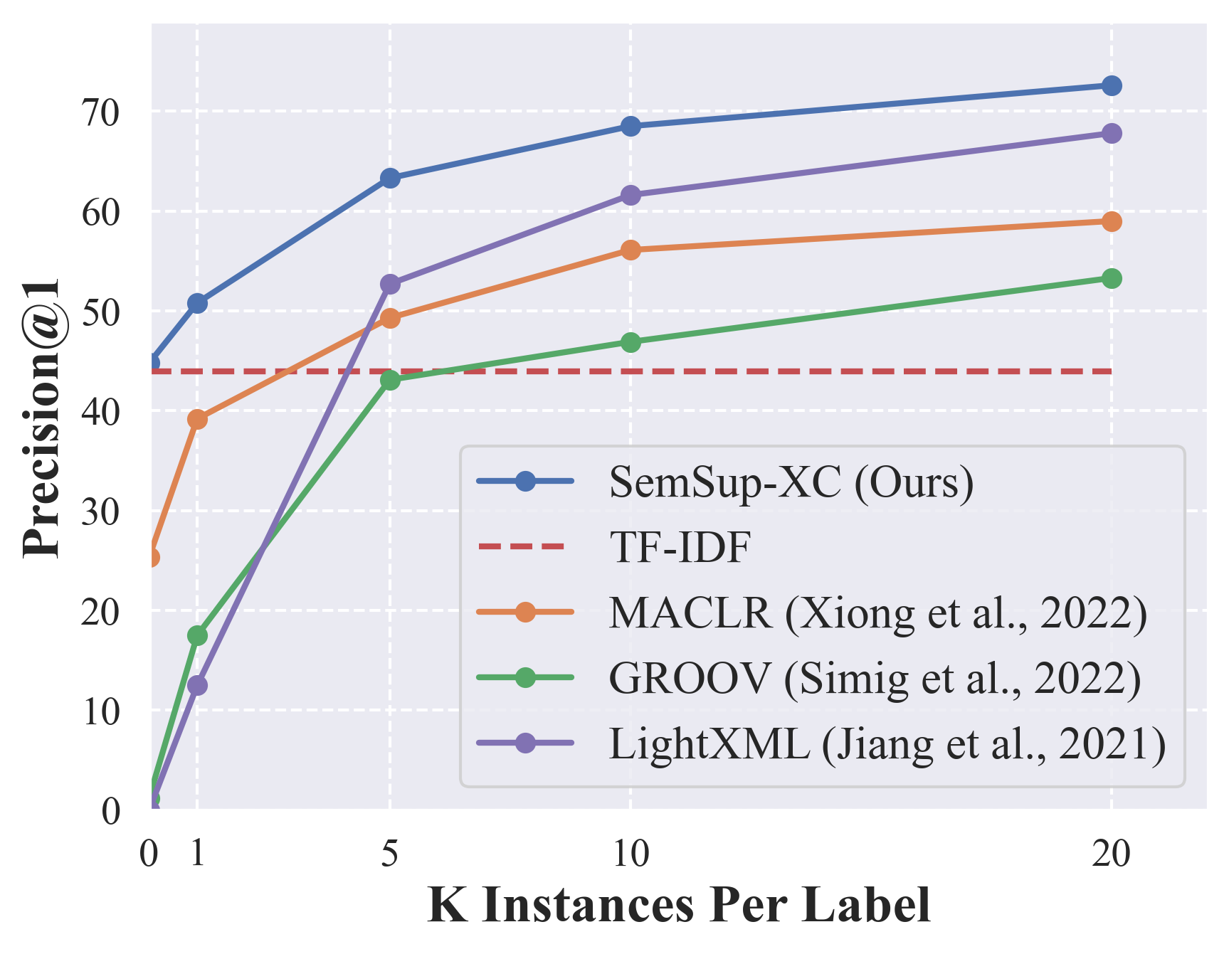
(a) EURLex-4.3K

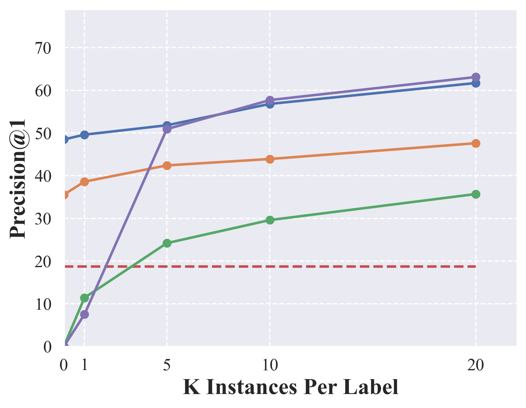
(b) AmazonCat-13K

Figure 2: Few-Shot P@1 for different Values of K on EURLex and AmazonCat. SemSup-XC starts off significantly higher and for EURLex maintains the gap for larger values of K to the second best model, MACLR Xiong2022ExtremeZL. For AmazonCat, SemSup-XC maintains similar leads for most baselines, while being at par with Light XML Jiang2021LightXMLTW.

4 Results

4.1 Zero-shot extreme classification

For the zero-shot scenario, we compare SemSup-XC with baselines which use class descriptions and counterparts which use class names as auxiliary information. We provide label hierarchy as additional supervision in both cases. We compare SemSup-XC with the best variant of each baseline. Table 2 shows that SemSup-XC significantly outperforms baselines on almost all datasets and metrics, under both zero-shot (ZS-XC) and generalized zero-shot (GZS-XC) settings. On ZS-XC, SemSup-XC outperforms MACLR by over $24$, $12$, and $6$ P@1 points on the three datasets respectively, even though MACLR uses XC specific pre-training. SemSup-XC also outperforms GROOV (e.g., over $48$ P@1 points on EURLex) which uses a generative T5 model pre-trained on significantly more data than our BERT backbone. GROOV’s unconstrained output space might be one of the reasons for its worse performance. SemSup-XC’s semantic understanding of instances and labels stands out against ZestXML which uses sparse non-contextual features with the former consistently scoring twice as higher compared to the latter. SemSup-XC consistently outperforms SPLADE (Formal2021SPLADESL), a state-of-the-art information retrieval method. This shows that the straightforward application of IR baselines on XC, even when they are fine-tuned, underperforms. This is likely because of the multi-label and fine-grained nature of classes coupled with a heavy-tailed distribution. For most of the datasets and settings, TF-IDF is competitive with deep baselines. This is because sparse methods often perform better than dense bi-encoders in zero-shot settings (Thakur2021BEIRAH), as the latter fail to capture fine-grained information. However, SemSup-XC’s hybrid lexico-semantic similarity module (Hybrid-Match) can perform fine-grained lexical and semantic matching between input instance and description and thus outperforms both sparse and deep methods on all datasets. SemSup-XC also outperforms the unsupervised baselines T5 and Sentence-Transformer, even though they are pre-trained on significantly larger amounts of data than BERT (T5 use $50\times$ compared our base model).

SemSup-XC also achieves higher recall on EURLex and AmazonCat datasets, beating the best performing baselines by $6$, $18$ R@10 points respectively, while being only 3 R@10 points less on Wikipedia. SemSup-XC is also the best model for GZS-XC. The margins of improvement are 1-2 P@1 points, which are smaller only because GZS-XC includes seen labels during evaluation, which are usually large in number. We refer readers to Appendix I.2 for more detailed discussion on GZS-XC performance. Table 7 in Appendix E contains additional results with more methods and metrics. Our results show that SemSup-XC is able to utilize the semantic and lexical information in class descriptions to improve performance significantly, while other baselines hardly improve when using descriptions instead of class names.

Method	Components				EURLex-4.3K			AmazonCat-13K
	Auxillary	Hierarchy	Exact	Hybrid	P@1	P@5	R@10	P@1	P@5	R@10
	Information		Match	Match
Ablating Label Descriptions
SemSup-XC	Descriptions	✓	✓	✓	$44.7$	$\mathbf{20.9}$	$\mathbf{57.4}$	$\bf{48.2}$	$\bf{27.0}$	$\bf{72.9}$
Replace descriptions with names	Names	✓	✓	✓	$\mathbf{45.4}$	$20.6$	$57.0$	$43.9$	$25.4$	$69.7$
Remove hierarchy	Descriptions	✗	✓	✓	$30.2$	$14.2$	$40.2$	$21.7$	$13.6$	$40.3$
Ablating Model Architecture Components
SemSup-XC	Descriptions	✓	✓	✓	$\mathbf{44.7}$	$\mathbf{20.9}$	$\mathbf{57.4}$	$\bf{48.2}$	$\bf{27.0}$	$\bf{72.9}$
Replace Hybrid with Exact Lexical Matching	Descriptions	✓	✓	✗	$42.6$	$19.3$	$53.7$	$45.8$	$25.5$	$69.2$
Remove all lexical matching	Descriptions	✓	✗	✗	$11.9$	$8.9$	$29.4$	$37.3$	$22.0$	$60.6$

Table 3: Component-wise Model Analysis of SemSup-XC for ZS-XC on EURLex and AmazonCat. Each component contributes to the final performance, with lexical-matching playing an important role.

Method	EURLex-4.3K			AmazonCat-13K
	P@1	P@5	R@10	P@1	P@5	R@10
SemSup-XC	$44.7$	$20.9$	$57.4$	$\bf{48.2}$	$\bf{27.0}$	$\bf{72.9}$
+ Augmentation	$\bf{45.5}$	$\bf{21.6}$	$\bf{59.0}$	$47.8$	$26.8$	$72.6$

Table 4: Description augmentation helps boost performance for ZS-XC on EURLex, but does not help on AmazonCat, which is a significantly larger dataset ($3\times$ labels). This demonstrates SemSup-XC’s out-of-the-box performance, since augmentation is unnecessary for larger label spaces.

4.2 Few-shot extreme classification

We now consider the FS-XC setup, where new classes added at evaluation time have a small number of labeled instances each ($K$). We evaluate on four settings – $K\in\{1,5,10,20\}$ and all baselines other than ZestXML, which cannot be used for FS-XC (See Appendix F). Further, we omit evaluation on Wikipedia, since it has $\approx 10$ training examples per label, which is insufficient to study the effect of increasing values of $K$. For the sake of completeness, we also include zero-shot performance (ZS-XC, $K=0$) and report results in Figure 2. Detailed results for other metrics (showing the same trend as P@1) and implementation details regarding creation of the few-shot splits are in appendix F.

Similar to the ZS-XC case, SemSup-XC outperforms all baselines for all values of $K$ on EURLex. For AmazonCat, SemSup-XC outperforms all baselines other than Light XML. Light XML is significantly outperformed for $K=\{0,1\}$ and matches for $K=\{5,10,20\}$. In comparison to MACLR and GROOV, SemSup-XC consistently outperforms by large margins (eg., 12 & 27P@1 points for EURLex) across all values of $K$. SemSup-XC’s zero-shot performance is higher than even the few-shot scores of MACLR and GROOV that have access to $K=20$ labeled samples on AmazonCat, which further strengthens the model’s applicability to the XC paradigm. Moreover, adding a few labeled examples seems to be more effective in EURLex than AmazonCat, with the performance difference between $K=1$ and $K=20$ being 22 and 12 P@1 points respectively. This, along with the fact that performance seems to plateau for both datasets, suggests that SemSup-XC learns label semantics better for AmazonCat than EURLex, due to its larger label space with rich descriptions.

4.3 Analysis

We dissect the performance of SemSup-XC by conducting ablation studies on model components and label descriptions and further provide qualitative analysis on EURLex and AmazonCat for the zero-shot extreme classification setting (ZS-XC) in the following sections.

Ablating components of SemSup-XC

Method	EURLex-4.3K			AmazonCat-13K
	P@1	P@5	R@10	P@1	P@5	R@10
WordNet	$42.8$	$20.7$	$55.0$	$47.2$	$26.2$	$72.2$
GPT-3 (6.7B)	$42.5$	$20.5$	$55.9$	$47.0$	$26.8$	$72.8$
SemSup-XC	$\bf{44.7}$	$\bf{20.9}$	$\bf{57.4}$	$\bf{48.2}$	$\bf{27.0}$	$\bf{72.9}$

Table 5: SemSup-XC significantly outperforms methods using descriptions from alternative sources like WordNet and GPT-3. Our approach consistently improves performance on EURLex and AmazonCat datasets. Additionally, our proposed method generates more diverse descriptions, scales efficiently to large datasets unlike LLM-based approaches, and provides descriptions for non-dictionary proper nouns, unlike WordNet.

Input Document	Top 5 Predictions
	SEMSUP-XC	MACLR
Start-Up: A Technician’s Guide. In addition to being an excellent stand-alone self-instructional guide, ISA recommends this book to prepare for the Start-Up Domain of CCST Level I, II, and III examinations.	test preparation	vocational tests
	schools & teaching	graduate preparation
	new	test prep & study guides
	used and rental textbooks	testing
	software	vocational
Homecoming (High Risk Books). When Katey Bruscke’s bus arrives in her unnamed hometown, she finds the scenery blurred, "as if my hometown were itself surfacing from beneath a black ocean." At …	literature & fiction	friendship
	thriller & suspense	mothers & children
	thrillers	drugs
	genre fiction	coming of age
	general	braille
Rolls RM65 MixMax 6x4 Mixer. The new RM65b HexMix is a single rack space unit featuring 6 channels of audio mixing, each with an XLR Microphone Input and 1/4ünbalanced Line Input. A unique …	studio recording equipment	powered mixers
	powered mixers	hand mixers
	home audio	mixers & accessories
	musical instruments	mixers
	speaker parts & components	mixer parts

Table 6: Sample predictions from SemSup-XC (our model) compared to MACLR (Xiong2022ExtremeZL). Bold represents correct predictions. Qualitative analysis shows that SemSup-XC can understand the document at a higher level than baselines like MACLR. The second example poses an especially interesting case where SemSup-XC is able to understand that the document is a fiction book, whereas MACLR tries to parse the story itself and predicts all labels incorrectly.

SemSup-XC’s use of the Hybrid-Match model and semantically rich descriptions enables it to outperform all baselines considered, and we analyze the importance of each component in Table 3. As our base model (first row) we consider SemSup-XC without ensembling it with TF-IDF. We note that the SemSup-XC base model is the best performing variant for both datasets and on all metrics other than P@1 for EURLex, for which it is only $0.7$ points lower. Web scraped class descriptions are important because removing them decreases both precision and recall scores (e.g., P@1 is lower by $4$ points on AmazonCat) on all settings considered. We see bigger improvements with AmazonCat, which is the dataset with larger number of classes (13K), which substantiates the need for semantically rich descriptions when dealing with a large number of fine-grained classes. Label hierarchy information is similarly crucial, with large performance drops on both datasets in its absence (e.g., $26$ P@1 points on AmazonCat), thus showing that access to structured hierarchy information leads to better semantic representations of labels.

On the modeling side, we observe that relaxed and exact lexical matching, which are components of Hybrid-Match, are important, with their absence leading to $2$ and $11$ P@1 point degradation on AmazonCat. Even for EURLex, hybrid lexical matching improves performance by $33$ P@1 points when compared to a model with no lexical matching. This highlights that our proposed model Hybrid-Match’s hybrid semantic-lexical approach significantly improves performance on XC datasets.

Augmenting Label Descriptions

The previous result showed the importance of class descriptions, and we explore the effect of augmenting them to increase their diversity and quantity (See Table 4). We use the easy data augmentation (EDA) method (eda) for augmentations. Specifically, we apply random word deletion, random word swapping, random insertion, and synonym replacement each with a probability of 0.5 on each description, and add the augmented descriptions to the original ones. We notice that augmentation improves performance on EURLex by $1$, $1$, and $2$ P@1, P@5, and R@10 points respectively, suggesting that augmentation can be a viable way to increase the quantity of descriptions. On AmazonCat, augmentation has no effect on the performance and rather slightly hurts it (e.g., $0.4$ P@1 points). Given that AmazonCat has $3\times$ the number of labels in EURLex, we believe this shows SemSup-XC’s effectiveness in capturing the label semantics in the presence of a larger number of classes, rendering data augmentation redundant. However, we believe that data augmentation might be a simple tool to boost performance on smaller datasets with lesser labels or descriptions.

4.4 Alternate Sources of Descriptions

We further assess the impact of utilizing class descriptions from various sources. In Table 5, we compare the performance of descriptions obtained from 1.) Language Model generated: We generate descriptions using variant of GPT-3 with 6.7B parameters, 2.) Knowledge Base: We use definitions provided in WordNet as descriptions, and 3.) SemSup-XC: Our proposed method. Our method consistently outperforms the others, with a 2 P@1 point improvement on EURLex and a 1 P@1 point improvement on AmazonCat. Furthermore, unlike LLM-based approaches, our method can efficiently scale to datasets containing millions of labels, such as Wikipedia. SemSup-XC generates more diverse descriptions compared to those available in WordNet and is also applicable to classes containing proper nouns or non-dictionary words. See Appendix I.1 for more details.

Qualitative analysis

We present a qualitative analysis of the performance SemSup-XC’s predictions in Table 6 compared to MACLR. Examples are instances where SemSup-XC outperforms MACLR, highlighting the strengths of our method, with correct predictions in bold. In the first example, while MACLR predicts five labels which are all similar, SemSup-XC is able to predict diverse labels while getting the correct label in five predictions. In the second example, SemSup-XC realizes the content of the document is a story and hence predicts literature & fiction, whereas MACLR predicts classes based on the content of the story instead. This shows the nuanced understanding of the label space that SemSup-XC has learned. In the third example, SemSup-XC shows a deep understanding of the label space by predicting "studio recording equipment" even though the document has no explicit mention of the words studio, recording or equipment. For same example, MACLR fails as it predicts labels like powered mixers because of the presence of the word mixer. These examples show that SemSup-XC’s understanding of how different fine-grained classes are related and how instances refer to them is better than the baselines considered. We list more such examples in Appendix H.

5 Related Work

Extreme classification

Extreme classification (XC) Agrawal2013MultilabelLW studies multi-class and multi-label classification problems over numerous classes (thousands to millions). Traditionally, studies have used sparse bag-of-words features of input documents (Bhatia2015SparseLE; Chang2019AMD; Lin2014MultilabelCV), simple one-versus-all binary classifiers (Babbar2017DiSMECDS; Yen2017PPDsparseAP; Jain2019SliceSL; dahiya2021siamesexml), and tree-based methods which utilize the label hierarchy (Parabel; Wydmuch2018ANG; Khandagale2020BonsaiDA). Recently, neural-network (NN) based contextual dense-features have improved accuracies. Studies have experimented with convolutional neural networks (Liu2017DeepLF), Transformers (xtransformer; Jiang2021LightXMLTW; zhang2021fast), attention-based networks (You2019AttentionXMLLT), and shallow networks (medini2019extreme; mittal2021decaf; dahiya2021deepxml). While the aforementioned works show impressive performance when the labels during training and testing are the same, they do not consider the practical zero-shot classification scenario with unseen test labels.

Zero-shot classification

Zero-shot classification (ZS) (larochelle2008zero) aims to predict unseen classes not encountered during training by utilizing auxiliary information like class names or prototypes. Multiple works have attempted ZS for text (dauphin2014zero; nam2016all; wang2018joint; pappas2019gile; Hanjie2022SemanticSE), however, they face performance degradation and are computationally expensive due to XC’s large label space. ZestXML (Gupta2021GeneralizedZE) was the first study to attempt ZS extreme classification by projecting non-contextual bag-of-words input features close to corresponding label features using a sparsified linear transformation. Subsequent works have used NNs to generate contextual representations (Xiong2022ExtremeZL; Simig2022OpenVE; zhang2022metadata; rios2018few), with MACLR (Xiong2022ExtremeZL) adding an XC specific pre-training step and GROOV (Simig2022OpenVE) using a sequence-to-sequence model to predict novel labels. However, these works use only label names to represent classes (e.g., the word “car”), which lack semantic information. We use semantically rich descriptions Hanjie2022SemanticSE, which coupled with our modeling innovations ($\S$ 2.2) achieves state-of-the-art performance on ZS-XC.

Computational Efficiency

In order to ensure efficient inference, similar to the training process, SemSup-XC makes predictions on the top 1000 labels shortlisted using TF-IDF. The results presented in Table 8 demonstrate that SemSup-XC achieves comparable throughput to deep baselines such as MACLR and GROOV, while significantly outperforming them in terms of overall performance. While ZestXML is significantly faster, SemSup-XC’s P@1 is $2\times$ higher. While SemSup-XC requires more storage, the modest 17 GB space it occupies on modern hard drives is inconsequential, especially considering the dataset’s scale, which comprises over a million labels. The storage requirements primarily stem from SemSup-XC’s Hybrid-Match module, which necessitates contextualized representations for each token in the description. These findings demonstrate that SemSup-XC strikes the optimal balance between throughput and performance while maintaining practical storage requirements. We provide a more detailed analysis of our method in Appendix G

6 Conclusion

We tackle the task of zero-shot extreme classification (XC) which involves very large label spaces, by using 1) Hybrid-Match, which incorporates both semantic similarity at the sentence level and relaxed lexical similarity at the token level, 2) contrastive learning to make training efficient, and 3) semantically rich class descriptions to gain a better understanding of the label space. We achieve state-of-the-art results on three standard XC benchmarks and significantly outperform prior work. Our various ablation studies and qualitative analyses demonstrate the relative importance of our modeling choices. Future work can further improve description quality, and given the strong performance of Hybrid-Match, can experiment with better architectures to further push the boundaries of this practical task.

7 Limitations

While our method, SemSup-XC, exhibits promising results, it is important to acknowledge its inherent limitations. Firstly, our approach relies on scraping descriptions from search engines. Although we have implemented post-processing techniques to filter out toxic content and retain only the most relevant search hits, it is possible that biases and harmful elements present in the original data may persist in the scraped descriptions. Furthermore, despite evaluating our method across diverse domains such as legal, shopping, and Wikipedia, it is essential to note that our approach may encounter challenges when applied to datasets where scraping descriptions is not a straightforward task or necessitates specialized technical knowledge that may not be readily available on the web.

Appendices

Appendix A Training Details

A.1 Hyperparameter Tuning

We tune the learning rate, batch_size using grid search. For the EURLex dataset, we use the standard validation split for choosing the best parameters. We set the input and output encoder’s learning rate at $5e^{-5}$ and $1e^{-4}$, respectively. We use the same learning rate for the other two datasets. We use batch_size of 16 on EURLex and 32 on AmazonCat and Wikipedia. For Eurlex, we train our zero-shot model for fixed 2 epochs and the generalized zero-shot model for 10 epochs. For the other 2 datasets, we train for a fixed 1 epoch. For baselines, we use the default settings as used in respective papers. For all daasets, we use same hyperparameters, and for baselines we use comparable settings to SemSup-XC for fair comparison.

Training

All of our models are trained end-to-end. We use the pretrained BERT model devlinbert for encoding input documents, and Bert-Small model Turc2019WellReadSL for encoding output descriptions. For efficiency in training, we freeze the first two layers of the output encoder. We use contrastive learning to train our models and sample hard negatives based on TF-IDF features. All implementation was done in PyTorch and Huggingface transformer and experiments were run NVIDIA RTX2080 and NVIDIA RTX3090 gpus.

A.2 Baselines

We use the code provided by ZestXML, MACLR and GROOV for running the supervised baselines. We employ the exact implementation of TF-IDF as used in ZestXML. We evaluate T5 as an NLI task (Xue2021mT5AM). We separately pass the names of each of the top 100 labels predicted by TF-IDF, and rank labels based on the likelihood of entailment. We evaluate Sentence-Transformer by comparing the similarity between the emeddings of input document and the names of the top 100 labels predicted by TF-IDF. Splade is a sparse neural retreival model that learns label/document sparse expansion via a Bert masked language modelling head. We use the code provided by authors for running the baselines. We experiment with various variations and pretrained models, and find splade_max_CoCodenser pretrained model with low sparsity($\lambda_{d}=1e-6$ & $\lambda_{q}=1e-6$) to be performing the best.

Appendix B Label descriptions from the web

B.1 Automatically scraping label descriptions from the web

We mine label descriptions from web in an automated end-to-end pipeline. We make query of the form ‘what is <class_name>’(or component name in case of Wikipedia) on duckduckgo search engine. Region is set to United States(English), and advertisements are turned off, with safe search set to moderate. We set time range from 1990 uptil June 2019. On average top 50 descriptions are scraped for each query. To further improve the scraped descriptions, we apply a series of heuristics:

• We remove any incomplete sentences. Incomplete sentences do not end in a period or do not have more than one noun, verb or auxiliary verb in them.
  Eg: Label = Adhesives ; Removed Sentence = What is the best glue or gel for applying

• Statements with lot of punctuation such as semi-colon were found to be non-informative. Descriptions with more than 10 non-period punctuations were removed.
  Eg: Label = Plant Cages & Supports ; Removed Description = Plant Cages & Supports. My Account; Register; Login; Wish List (0) Shopping Cart; Checkout $ USD $ AUD THB; R$ BRL $ CAD $ CLP $ …

• We used regex search to identify urls and currencies in the text. Most of such descriptions were spam and were removed.
  Eg: Label = Accordion Accessories ; Removed Description = Buy Accordion Accessories Online, with Buy Now & Pay Later and Rental Options. Free Shipping on most orders over $250. Start Playing Accordion Accessories Today!

• Descriptions with small sentences(<5 words) were removed.
  Eg: Label = Boats ; Removed Description = Boats for Sale. Buy A Boat; Sell A Boat; Boat Buyers Guide; Boat Insurance; Boat Financing …

• Descriptions with more than 2 interrogative sentences were filtered out.
  Eg: Label = Shower Curtains ; Removed Description = So you’re interested…why? you’re starting a company that makes shower curtains? or are you just fooling around? Wiki User 2010-04

• We mined top frequent n-grams from a sample of scraped descriptions, and based on it identified n-grams which were commonly used in advertisements. Examples include: ‘find great deals’, ‘shipped by’.
  Label = Boat compasses ; Removed Description = Shop and read reviews about Compasses at West Marine. Get free shipping on all orders to any West Marine Store near you today.

• We further remove obscene words from the datasets using an open-source library (profanity).

• We also run a spam detection model (spamdet) on the descriptions and remove those with a confidence threshold above 0.9.
  Eg: Label = Phones ; Removed Description = Check out the Phones page at <xyz_company> — the world’s leading music technology and instrument retailer!

• Additionally, most of the sentences in first person, were found to be advertisements, and undetected by previous model. We remove descriptions with more than 3 first person words (such as I, me, mine) were removed.
  Eg: Label = Alarm Clocks ; Removed Description = We selected the best alarm clocks by taking the necessary, well, time. We tested products with our families, waded our way through expert and real-world user opinions, and determined what models lived up to manufacturers’ claims. …

B.2 Post-Processing

We further add hierarchy information in a natural language format to the label descriptions for AmazonCat and EURLex datasets. Precisely, we follow the format of ‘key is value.’ with each key, value pair represented in new line. Here key belongs to the set { ‘Description’, ‘Label’, ‘Alternate Label Names’, ‘Parents’, ‘Children’ }, and the value corresponds to comma separated list of corresponding information from the hierarchy or scraped web description. For example, consider the label ‘video surveillance’ from EURLex dataset. We pass the text:
‘Label is video surveillance.
Description is <web_scraped_description>.
Parents are video communications.
Alternate Label Names are camera surveillance, security camera surveillance.’
to the output encoder.
For Wikipedia, label hierarchy is not present, so we only pass the description along with the name of label.

B.3 Wikipedia Descriptions

When labels are fine-grained, as in the Wikipedia dataset, making queries for the full label name is not possible. For example, consider the label ‘Fencers at the 1984 Summer Olympics’ from Wikipedia categories; querying for it would link to the same category on Wikipedia itself. Instead, we break the label names into separate constituents using a dependency parser. Then for each constituent(‘Fencers’ and ‘Summer Olympics’), we scrape descriptions. No descriptions are scraped for constituents labelled by Named-Entity Recognition(‘1984’), and their NER tag is directly used. Finally, all the scraped descriptions are concatenated in a proper format and passed to the output encoder.

B.4 De-Duplication

To ensure no overlap between our descriptions and input documents, we used SuffixArray-based exact match algorithm  (Lee2022DeduplicatingTD) with a minimum threshold of 60 characters and removed the matched descriptions.

Appendix C Hybrid-Match

We propose Hybrid-Match to exploit token similarity. We create clusters of tokens based on: 1) the BERT token-embedding similarity (Rajaee2021ACAisotropic) is higher than a threshold or 2) if tokens share the same lemma. Specifically, first tokens with BERT embedding cosine similarity greater than 0.6 are put into same cluster. In the second stage if two different tokens share the same lemma, but are in different clusters, their clusters are merged. In model, a mask is created of size (Q * LQ * D * LD), where Q is the number of label descriptions, LQ is the max length of all label descriptions, D is the number of documents, and LD is the length of label descriptions. Here a entry of 1 means that corresponding token in label description and input share the same cluster, else it is set to 0.

Appendix D Contrastive Learning

During training, for both EURLex and AmazonCat, we sample $1000-|Y_{i}^{+}|$ hard negative labels for each input document. For Wikipedia, we precompute the top 1000 labels for each input based on TF-IDF scores. We then randomly sample $1000-|Y_{i}^{+}|$ negative labels for each document. At inference time, we evaluate our models on all labels for both EURLex and AmazonCat. However, even evaluation on millions of labels in Wikipedia is not computationally tractable. Therefore, we evaluate only on top 1000 labels predicted by TF-IDF for each input.

Appendix E Full results for zero-shot classification

E.1 Split Creation

For EURLex, and AmazonCat, we follow the same procedure as detailed in GROOV (Simig2022OpenVE). We randomly sample k labels from all the labels present in train set, and consider the remaining labels as unseen. For EURLex we have roughly 25%(1057 labels) and for AmazonCat roughly 50%(6500 labels) as unseen. For Wikipedia, we use the standard splits as proposed in ZestXML (Gupta2021GeneralizedZE).

E.2 Results

Table 7 contains complete results for ZS-XCacross the three datasets, including additional baselines and metrics.

Method	Precision - ZSL			Recall - ZSL / GZSL		Precision - GZSL
	$@1$	$@3$	$@5$	$R@10$	$R@10$	$@1$	$@3$	$@5$
Eurlex-4.3K
TF-IDF	$44.0$$(\pm 0.0)$	$26.9$$(\pm 0.0)$	$19.6$$(\pm 0.0)$	$55.8$$(\pm 0.0)$	$41.2$$(\pm 0.0)$	$53.4$$(\pm 0.0)$	$35.2$$(\pm 0.0)$	$28.0$$(\pm 0.0)$
T5	$7.2$$(\pm 0.0)$	$7.1$$(\pm 0.0)$	$7.0$$(\pm 0.0)$	$29.2$$(\pm 0.0)$	$23.0$$(\pm 0.0)$	$10.4$$(\pm 0.0)$	$11.0$$(\pm 0.0)$	$11.2$$(\pm 0.0)$
Sentence Transformer	$15.9$$(\pm 0.0)$	$10.8$$(\pm 0.0)$	$9.1$$(\pm 0.0)$	$31.1$$(\pm 0.0)$	$25.5$$(\pm 0.0)$	$18.8$$(\pm 0.0)$	$15.7$$(\pm 0.0)$	$11.9$$(\pm 0.0)$
ZestXML	$9.6$$(\pm 0.0)$	$7.3$$(\pm 0.0)$	$6.5$$(\pm 0.0)$	$25.7$$(\pm 0.0)$	$54.8$$(\pm 0.0)$	$84.8$$(\pm 0.0)$	$64.8$$(\pm 0.0)$	$48.9$$(\pm 0.0)$
ZestXML + TF-IDF	$24.7$$(\pm 0.0)$	$17.7$$(\pm 0.0)$	$14.4$$(\pm 0.0)$	$46.4$$(\pm 0.0)$	$54.2$$(\pm 0.0)$	$84.9$$(\pm 0.0)$	$65.7$$(\pm 0.0)$	$50.3$$(\pm 0.0)$
MACLR	$24.9$$(\pm 0.6)$	$16.6$$(\pm 0.2)$	$13.4$$(\pm 0.2)$	$42.1$$(\pm 0.5)$	$55.2$$(\pm 1.3)$	$60.7$$(\pm 1.3)$	$49.1$$(\pm 1.9)$	$41.1$$(\pm 1.3)$
GROOV	$1.2$ $(\pm 0.1)$	$2.6$ $(\pm 0.4)$	$2.6$ $(\pm 0.3)$	$7.0$ $(\pm 0.9)$	$49.4$ $(\pm 0.1)$	$84.1$ $(\pm 0.1)$	$61.5$ $(\pm 0.2)$	$45.3$ $(\pm 0.1)$
SemSup-XC-Hier	$45.4$$(\pm 0.2)$	$28.1$$(\pm 0.1)$	$20.6$$(\pm 0.2)$	$57.0$$(\pm 0.2)$	$65.6$$(\pm 1.0)$	$86.4$$(\pm 0.2)$	$\mathbf{69.2}$$(\pm 0.2)$	$\mathbf{54.2}$$(\pm 0.4)$
SemSup-XC	$44.7$$(\pm 2.3)$	$27.9$$(\pm 1.1)$	$20.9$$(\pm 0.6)$	$57.4$$(\pm 3.4)$	$\mathbf{65.2}$$(\pm 0.3)$	$\mathbf{87.1}$$(\pm 0.1)$	$68.5$$(\pm 0.1)$	$53.7$$(\pm 0.1)$
SemSup-XC + TF-IDF	$\mathbf{49.3}$$(\pm 0.9)$	$\mathbf{31.2}$$(\pm 0.8)$	$\mathbf{23.1}$$(\pm 0.3)$	$\mathbf{62.4}$$(\pm 0.8)$	$62.9$$(\pm 1.1)$	$87.0$$(\pm 0.1)$	$67.6$$(\pm 0.1)$	$51.6$$(\pm 0.6)$
Amazon-13K
TF-IDF	$18.7$$(\pm 0.0)$	$11.5$$(\pm 0.0)$	$8.5$$(\pm 0.0)$	$21.0$$(\pm 0.0)$	$14.7$$(\pm 0.0)$	$21.5$$(\pm 0.0)$	$14.4$$(\pm 0.0)$	$11.1$$(\pm 0.0)$
T5	$2.5$$(\pm 0.0)$	$2.8$$(\pm 0.0)$	$3$$(\pm 0.0)$	$10.5$$(\pm 0.0)$	$10.2$$(\pm 0.0)$	$3.2$$(\pm 0.0)$	$4.2$$(\pm 0.0)$	$4.9$$(\pm 0.0)$
Sentence Transformer	$15.2$$(\pm 0.0)$	$10.5$$(\pm 0.0)$	$8.3$$(\pm 0.0)$	$22.2$$(\pm 0.0)$	$16.0$$(\pm 0.0)$	$18.4$$(\pm 0.0)$	$13.4$$(\pm 0.0)$	$11.0$$(\pm 0.0)$
ZestXML	$12.7$$(\pm 0.0)$	$8.9$$(\pm 0.0)$	$7.1$$(\pm 0.0)$	$21.2$$(\pm 0.0)$	$52.5$$(\pm 0.0)$	$87.9$$(\pm 0.0)$	$58.6$$(\pm 0.0)$	$41.5$$(\pm 0.0)$
ZestXML + TF-IDF	$15.6$$(\pm 0.0)$	$11.1$$(\pm 0.0)$	$8.8$$(\pm 0.0)$	$24.4$$(\pm 0.0)$	$54.2$$(\pm 0.0)$	$87.6$$(\pm 0.0)$	$59.0$$(\pm 0.0)$	$42.3$$(\pm 0.0)$
MACLR	$36.0$$(\pm 0.6)$	$23.5$$(\pm 0.4)$	$18.0$$(\pm 0.4)$	$54.4$$(\pm 0.8)$	$46.9$$(\pm 0.4)$	$46.0$$(\pm 0.3)$	$33.7$$(\pm 0.3)$	$27.2$$(\pm 0.3)$
GROOV	$0.0$$(\pm 0.0)$	$0.3$$(\pm 0.0)$	$0.5$$(\pm 0.0)$	$2.4$ $(\pm 0.2)$	$47.9$$(\pm 0.3)$	$87.4$$(\pm 0.5)$	$55.8$$(\pm 0.8)$	$38.8$$(\pm 0.5)$
SemSup-XC-Hier	$43.9$$(\pm 0.4)$	$31.5$$(\pm 0.7)$	$25.4$$(\pm 0.3)$	$69.7$$(\pm 0.6)$	$71.5$$(\pm 0.3)$	$88.4$$(\pm 0.3)$	$65.0$$(\pm 0.5)$	$50.2$$(\pm 0.3)$
SemSup-XC + TF-IDF	$\mathbf{48.2}$$(\pm 0.5)$	$\mathbf{33.9}$$(\pm 0.2)$	$\mathbf{27.0}$$(\pm 0.5)$	$\mathbf{72.9}$$(\pm 0.5)$	$\mathbf{71.6}$$(\pm 0.3)$	$\mathbf{88.6}$$(\pm 0.1)$	$\mathbf{65.3}$$(\pm 0.3)$	$\mathbf{51.2}$$(\pm 0.1)$
Wikipedia-1M
TF-IDF	$14.5$$(\pm 0.0)$	$7.7$$(\pm 0.0)$	$5.5$$(\pm 0.0)$	$18.3$$(\pm 0.0)$	$14.7$$(\pm 0.0)$	$14.4$$(\pm 0.0)$	$8.5$$(\pm 0.0)$	$6.5$$(\pm 0.0)$
T5	$8.2$$(\pm 0.0)$	$7.6$$(\pm 0.0)$	$6.7$$(\pm 0.0)$	$23.6$$(\pm 0.0)$	$15.1$$(\pm 0.0)$	$4.2$$(\pm 0.0)$	$4.5$$(\pm 0.0)$	$4.4$$(\pm 0.0)$
Sentence Transformer	$19.6$$(\pm 0.0)$	$11.1$$(\pm 0.0)$	$7.9$$(\pm 0.0)$	$22.5$$(\pm 0.0)$	$16.6$$(\pm 0.0)$	$14.2$$(\pm 0.0)$	$9.1$$(\pm 0.0)$	$7.0$$(\pm 0.0)$
ZestXML	$12.9$$(\pm 0.0)$	$8.0$$(\pm 0.0)$	$6.0$$(\pm 0.0)$	$20.0$$(\pm 0.0)$	$25.7$$(\pm 0.0)$	$26.7$$(\pm 0.0)$	$18.8$$(\pm 0.0)$	$14.6$$(\pm 0.0)$
ZestXML + TF-IDF	$15.8$$(\pm 0.0)$	$8.9$$(\pm 0.0)$	$6.4$$(\pm 0.0)$	$20.8$$(\pm 0.0)$	$26.3$$(\pm 0.0)$	$30.6$$(\pm 0.0)$	$22.2$$(\pm 0.0)$	$17.2$$(\pm 0.0)$
MACLR	$29.8$$(\pm 0.8)$	$17.8$$(\pm 0.6)$	$13.2$$(\pm 0.4)$	$\mathbf{41.7}$$(\pm 1.3)$	$32.7$$(\pm 0.6)$	$28.0$$(\pm 0.3)$	$18.3$$(\pm 0.3)$	$14.4$$(\pm 0.4)$
GROOV	$6.0$$(\pm 0.1)$	$5.8$$(\pm 0.3)$	$5.0$$(\pm 0.4)$	$15.4$$(\pm 0.2)$	$29.0$$(\pm 0.2)$	$31.4$$(\pm 0.1)$	$\mathbf{24.9}$$(\pm 0.1)$	$\mathbf{19.1}$$(\pm 0.0)$
SemSup-XC	$34.6$$(\pm 0.2)$	$18.9$$(\pm 0.2)$	$13.1$$(\pm 0.3)$	$37.9$$(\pm 0.4)$	$33.0$$(\pm 0.3)$	$29.8$$(\pm 0.1)$	$22.0$$(\pm 0.2)$	$17.0$$(\pm 0.4)$
SemSup-XC + TF-IDF	$\mathbf{36.5}$$(\pm 0.3)$	$\mathbf{19.5}$$(\pm 0.2)$	$\mathbf{13.4}$$(\pm 0.5)$	$38.5$$(\pm 0.3)$	$\mathbf{34.1}$$(\pm 0.3)$	$\mathbf{33.7}$$(\pm 0.4)$	$23.4$$(\pm 0.3)$	$17.7$$(\pm 0.2)$

Table 7: Comparison of SEMSUP-XC with other supervised and unsupervised baselines. Our method consistently outperfoms all methods across all datasets.

Model	Device	Throughput	Storage	P@1
		(Inputs/s)	(GB)	(ZSL)
SemSup-XC	1 GPU	$46.2$	$17.9$	$\mathbf{36.5}$
MACLR	1 GPU	$77.8$	$4.6$	$29.8$
GROOV	1 GPU	$8.9$	$\mathbf{0.4}$	$6.0$
ZestXML	16 CPUs	$\mathbf{2371}$	$1.8$	$15.8$

Table 8: Computational Efficiency of SemSup-XC and baselines on Wikipedia dataset. We have comparable throughput to dense baselines while requiring higher storage but with substantial performance gains.

Appendix F Full results for few-shot classification

F.1 Split Creation

We iteratively select k instances of each label in train documents. If a label has more than k documents associated with it, we drop the label from training(such labels are not sampled as either positives or negatives) for the extra documents. We refer to these labels as neutral labels for convenience. Because of such labels, loss functions of dense methods need to be modified accordingly. For ZestXML, this is not possible because it directly learns a transformation over the whole dataset, and individual labels for particular instances cannot be masked as neutral.

F.2 Models

We use MACLR, GROOV, Light XML as baselines. We initialize the weights from the corresponding pre-trained models in the GZSL setting. We use the default hyperparameters for baselines and semsup models. As discussed in the previous section, neutral labels are not provided at train time for MACLR and GROOV baselines. However, since Light XML uses a final fully-connected classification layer, we cannot selectively remove them for a particular input. Therefore, we mask the loss for labels which are neutral to the documents. We additionally include scores for TF-IDF, but since it is a fully unsupervised method, only zero-shot numbers are included.

F.3 Results

The full results for few-shot classification are present in Table 9.

Method	EURLex-4.3K			AmazonCat-13K
	P@1	P@5	R@10	P@1	P@5	R@10
1-shot
SemSup-XC	$\mathbf{50.8}$$(\pm 0.9)$	$\mathbf{21.4}$$(\pm 0.7)$	$\mathbf{57.9}$$(\pm 2.9)$	$\mathbf{49.6}$$(\pm 0.4)$	$\mathbf{25.2}$$(\pm 0.2)$	$\mathbf{66.3}$$(\pm 0.7)$
MACLR	$39.2$$(\pm 0.7)$	$17.3$$(\pm 0.5)$	$50.9$$(\pm 1.0)$	$38.6$$(\pm 0.6)$	$19.7$$(\pm 0.1)$	$56.4$$(\pm 0.8)$
MACLR with Descriptions	$38.5$$(\pm 0.4)$	$17.0$$(\pm 0.5)$	$49.1$$(\pm 0.8)$	$36.3$$(\pm 0.4)$	$18.3$$(\pm 0.7)$	$52.4$$(\pm 0.6)$
GROOV	$17.5$$(\pm 0.6)$	$4.2$$(\pm 0.2)$	$9.4$$(\pm 0.4)$	$11.4$$(\pm 0.8)$	$4.3$$(\pm 0.4)$	$9.1$$(\pm 0.9)$
GROOV with Descriptions	$1.1$$(\pm 0.2)$	$0.4$$(\pm 0.2)$	$1.3$$(\pm 0.3)$	$4.0$$(\pm 0.3)$	$0.9$$(\pm 0.1)$	$1.9$$(\pm 0.4)$
Light XML	$12.5$$(\pm 1.9)$	$6.3$$(\pm 0.9)$	$19.5$$(\pm 2.9)$	$7.5$$(\pm 0.7)$	$7.0$$(\pm 0.3)$	$25.1$$(\pm 0.3)$
5-shot
SemSup-XC	$\mathbf{63.3}$$(\pm 0.3)$	$\mathbf{26.3}$$(\pm 0.3)$	$\mathbf{67.6}$$(\pm 0.1)$	$\mathbf{51.8}$$(\pm 0.1)$	$\mathbf{26.1}$$(\pm 0.2)$	$\mathbf{70.0}$$(\pm 0.8)$
MACLR	$51.2$$(\pm 0.4)$	$23.0$$(\pm 0.2)$	$63.8$$(\pm 0.7)$	$42.4$$(\pm 0.3)$	$21.6$$(\pm 0.4)$	$61.4$$(\pm 0.1)$
MACLR with Descriptions	$52.5$$(\pm 0.4)$	$22.9$$(\pm 0.5)$	$62.1$$(\pm 0.4)$	$39.3$$(\pm 0.5)$	$19.9$$(\pm 0.3)$	$57.4$$(\pm 0.6)$
GROOV	$43.1$$(\pm 1.0)$	$14.2$$(\pm 0.5)$	$33.3$$(\pm 1.1)$	$24.2$$(\pm 0.8)$	$9.7$$(\pm 0.6)$	$19.4$$(\pm 1.5)$
GROOV with Descriptions	$6.0$$(\pm 0.6)$	$1.3$$(\pm 0.4)$	$3.5$$(\pm 0.6)$	$17.6$$(\pm 0.5)$	$3.5$$(\pm 0.2)$	$9.5$$(\pm 0.3)$
Light XML	$52.7$$(\pm 0.1)$	$23.7$$(\pm 0.0)$	$62.6$$(\pm 0.3)$	$50.9$$(\pm 0.7)$	$24.7$$(\pm 0.4)$	$64.3$$(\pm 0.4)$
10-shot
SemSup-XC	$\mathbf{68.5}$$(\pm 0.1)$	$\mathbf{28.3}$$(\pm 0.5)$	$\mathbf{71.9}$$(\pm 2.1)$	$56.8$$(\pm 0.3)$	$\mathbf{27.7}$$(\pm 0.4)$	$\mathbf{69.8}$$(\pm 0.5)$
MACLR	$56.1$$(\pm 0.1)$	$25.4$$(\pm 0.0)$	$69.4$$(\pm 0.1)$	$43.9$$(\pm 0.2)$	$22.3$$(\pm 0.0)$	$62.9$$(\pm 0.3)$
MACLR with Descriptions	$57.0$$(\pm 0.2)$	$26.7$$(\pm 0.3)$	$69.7$$(\pm 0.3)$	$41.6$$(\pm 0.3)$	$21.4$$(\pm 0.2)$	$60.3$$(\pm 0.5)$
GROOV	$46.9$$(\pm 0.6)$	$18.0$$(\pm 0.1)$	$43.2$$(\pm 0.2)$	$29.6$$(\pm 0.4)$	$12.8$$(\pm 0.1)$	$29.3$$(\pm 0.4)$
GROOV with Descriptions	$10.1$$(\pm 0.4)$	$2.0$$(\pm 0.1)$	$4.8$$(\pm 0.4)$	$21.4$$(\pm 0.5)$	$4.5$$(\pm 0.5)$	$13.4$$(\pm 0.4)$
Light XML	$61.6$$(\pm 0.6)$	$27.1$$(\pm 0.3)$	$71.0$$(\pm 0.4)$	$\mathbf{57.7}$$(\pm 0.3)$	$27.5$$(\pm 0.3)$	$69.3$$(\pm 0.7)$
20-shot
SemSup-XC	$\mathbf{72.6}$$(\pm 0.2)$	$\mathbf{30.8}$$(\pm 0.1)$	$\mathbf{78.2}$$(\pm 0.4)$	$61.7$$(\pm 0.5)$	$\mathbf{29.9}$$(\pm 0.2)$	$\mathbf{73.9}$$(\pm 0.3)$
MACLR	$59.0$$(\pm 0.3)$	$27.2$$(\pm 0.0)$	$73.2$$(\pm 0.2)$	$47.6$$(\pm 0.2)$	$24.1$$(\pm 0.1)$	$66.9$$(\pm 0.3)$
MACLR with Descriptions	$60.6$$(\pm 0.5)$	$27.4$$(\pm 0.4)$	$73.2$$(\pm 0.4)$	$47.2$$(\pm 0.3)$	$23.5$$(\pm 0.2)$	$66.3$$(\pm 0.2)$
GROOV	$53.3$$(\pm 1.3)$	$21.5$$(\pm 0.8)$	$52.7$$(\pm 2.2)$	$35.7$$(\pm 0.2)$	$15.6$$(\pm 0.2)$	$39.5$$(\pm 0.3)$
GROOV with Descriptions	$16.4$$(\pm 0.3)$	$3.6$$(\pm 0.4)$	$10.0$$(\pm 0.6)$	$29.0$$(\pm 0.3)$	$6.4$$(\pm 0.4)$	$18.1$$(\pm 0.4)$
Light XML	$67.8$$(\pm 0.5)$	$30.4$$(\pm 0.1)$	$76.6$$(\pm 0.0)$	$\mathbf{63.1}$$(\pm 0.2)$	$29.8$$(\pm 0.3)$	$73.6$$(\pm 0.3)$

Table 9: Detailed table for few-shot results. SemSup-XC outperforms all other baselines with significant margins for $k=1,5,\&10$ shot settings. For 20-shot we perform almost at par with fully supervised method of Light XML, which otherwise performs poorly for zero-shot and lower values of k in few shot setting.

Appendix G Computational Efficiency

Extreme Classification necessitates that the models scale well in terms of time and memory efficiency with labels at both train and test times. SemSup-XC uses contrastive learning for efficiency at train time. During inference, SemSup-XC predicts on top 1000 shortlists by TF-IDF, thereby achieving sub-linear time. Further, contextualized tokens for label descriptions are computed only once and stored in memory-mapped files, thus decreasing computational time significantly. Overall, our computational complexity can be represented by $\mathcal{O}(T_{IE}*N+T_{OE}*|Y|+k*N*T_{lex})$, where $T_{IE}$, $T_{OE}$ represent the time taken by input encoder and output encoder respectively, $N$ is the total number of input documents, |Y| is the number of all labels, k indicates the shortlist size and $|T_{lex}|$ denotes the time in soft-lexical computation between contextualized tokens of documents and labels. In our experiments, $T_{IE}*N>>T_{OE}*|Y|$ and $T_{IE}\approx T_{lex}*k$. Thus effectively, computational complexity is approximately equal to $\mathcal{O(T_{IE}*N)}$, which is in comparison to other SOTA extreme classification methods.

To ensure efficiency at inference time, similar to training, SemSup-XC predicts on top of 1000 labels shortlisted by TF-IDF. Table 8 shows that SemSup-XC’s throughput is comparable to deep baselines (MACLR and GROOV) while demonstrating much better performance. While ZestXML is significantly faster, SemSup-XC’s P@1 is $2\times$ higher. While SemSup-XC’s storage is higher, $17$ GB of space on modern-day hard drives is trivial, especially given that the dataset has over a million labels. SemSup-XC’s Hybrid-Match module requires contextualized representations for every token in the description, which contributes to the majority of the storage. This shows that SemSup-XC provides the best throughput-performance trade-off while having practical storage requirements.

Method	Eurlex P@1	Eurlex R@10	Amazon P@1	Amazon R@10	Wiki P@1	Wiki R@10
ZestXML	$84.9$	$60.2$	$87.6$	$54.2$	$26.3$	$17.2$
MACLR	$60.7$	$55.2$	$46.0$	$46.9$	$28.0$	$32.7$
GROOV	$84.1$	$49.4$	$87.4$	$47.9$	$31.4$	$29.0$
SemSup-XC	$87.0$	62.9	$88.6$	71.6	$33.7$	$34.1$
$Oracle_{\text{Seen}}$	97.2	$60.0$	95.0	$54.9$	66.1	43.2

Table 10: Comparison of $Oracle_{Seen}$ on GZS-XC split. $Oracle_{Seen}$ is able to get high scores, despite completely ignoring unseen labels. However SemSup-XC is the only method that beats $Oracle_{Seen}$ by significant margins on EURLex and AmazonCat datasets.

Method	$P(D_{unseen},Y)@1$	$R(D_{unseen},Y)@10$
GROOV	$0.0$	$0.8$
ZestXML	$0.2$	$8.8$
MACLR	$16.4$	$23.7$
SemSup-XC	31.2	36.8

Table 11: Comparison of $P(D_{unseen},Y)$ and $R(D_{unseen},Y)$ on GZS-XC split on EURLex dataset. GROOV and ZestXML perform very poorly demonstrating they are deriving high scores on GZS-XC solely from seen labels. MACLR performs decently, while SemSup-XC performs the best indicating the contribution of unseen labels in it’s high scores in GZS-XC setting.

Appendix H Qualitative Analysis

Table 12 shows multiple qualitative examples for which our model outperforms the next baseline MACLR. The examples were chosen so as to increase diversity of input document’s topic, number of correct predictions and relative improvement over baseline. All examples are on AmazonCat dataset.

Input Document	Top 5 Predictions
	SEMSUP-XC	MACLR
Start-Up: A Technician’s Guide. In addition to being an excellent stand-alone self-instructional guide, ISA recommends this book to prepare for the Start-Up Domain of CCST Level I, II, and III examinations.	test preparation	vocational tests
	schools & teaching	graduate preparation
	new	test prep & study guides
	used and rental textbooks	testing
	software	vocational
Homecoming (High Risk Books). When Katey Bruscke’s bus arrives in her unnamed hometown, she finds the scenery blurred, "as if my hometown were itself surfacing from beneath a black ocean." At the conclusion of new novelist Gussoff’s "day-in-the-life-of" first-person narrative, the reader feels equally blurred by the relentless …	literature & fiction	friendship
	thriller & suspense	mothers & children
	thrillers	drugs
	genre fiction	coming of age
	general	braille
Rolls RM65 MixMax 6x4 Mixer. The new RM65b HexMix is a single rack space unit featuring 6 channels of audio mixing, each with an XLR Microphone Input and 1/4ünbalanced Line Input. A unique feature of the 1/4l̈ine inputs is they may be internally reconfigured to operate as Inserts for the Microphone Input. Each channel, in …	studio recording equipment	powered mixers
	powered mixers	hand mixers
	home audio	mixers & accessories
	musical instruments	mixers
	speaker parts & components	mixer parts
Political Business in East Asia (Politics in Asia). The book offers a valuable analysis of the ties between politics and business in various East Asian countries..Pacific Affairs, Fall 2003	international & world politics	international
	business & investing	relations
	politics & social sciences	policy & current events
	asian	practical politics
	economics	international law
Chicago Latrobe 550 Series Cobalt Steel Jobber Length Drill Bit Set with Metal Case, Gold Oxide Finish, 135 Degree Split Point, Wire Size, 60-piece, #60 - #1. This Chicago-Latrobe 550 series jobber length drill bit set contains 60 cobalt steel drill bits, including one each of wire gauge sizes #60 through #1, with a gold oxide finish and a …	drill bits	industrial drill bits
	twist drill bits	step drill bits
	power & hand tools	long length drill bits
	jobber drill bits	reduced shank drill bits
	power tool accessories	installer drill bits
Raggedy Ann and Johnny Gruelle: A Bibliography of Published Works. Patricia Hall has written and lectured extensively on Gruelle and his contributions to American culture. Her collection of Gruelle’s books, dolls, correspondence, original artwork, business records and photographs is one of the most comprehensive in the world. Many …	reference	art
	history & criticism	bibliographies & indexes
	humor & entertainment	art & photography
	publishing & books	arts
	research & publishing guides	children’s literature
Harmonic Analysis and Applications (Studies in Advanced Mathematics). The present book may definitely be useful for anyone looking for particular results, examples, applications, exercises, or for a book that provides the skeleton for a good course on harmonic analysis. R. Brger; Monatsheft fr Mathematik; 127.1999.3	statistics	pure mathematics
	science & math	algebra
	professional science	applied
	new	algebra & trigonometry
	used & rental textbooks	calculus
Soldier Spies: Israeli Military Intelligence. After its brilliant successes in the Six-Day War, the War of Attrition and the campaign against Black September, A’MAN, Israel’s oldest intelligence agency, fell prey to institutional hubris. A’MAN’s dangerous overconfidence only deepened, Katz here reveals, after spectacular coups such as …	israel	intelligence & espionage
	middle east	espionage
	international & world politics	national & international security
	politics & social sciences	middle eastern
	history	arms control
SF Signature White Chocolate Fondue, 4-Pound (Pack of 2). Smooth and creamy SF Signature White Chocolate Fondue provides unparalleled flavor in an incredibly easy-to-use product. This white chocolate fondue works better than other fountain chocolates due to its low viscosity and great taste. Packaged in two pound …	chocolate	baking cocoa
	breads & bakery	chocolate truffles
	pantry staples	chocolate assortments
	canned & jarred food	baking chocolates
	kitchen & dining	chocolate
Little Monsters: Monster Friends and Family (1000). Kind of a demented Monsters, Inc. meets Oliver Twist, the 1989 live-action film Little Monsters takes every child’s nightmare of a monster under the bed and spins it into a dark tale of a secret underworld where children and adults turn into monsters and run wild without rules or any …	movies & tv	movies
	film	movies & tv
	musical genres	tv
	rock	film
	tv	theater
adidas Women’s Ayuna Sandal,Newnavy/Wht/Altitude,5 M. adidas is a name that stands for excellence in all sectors of sport around the globe. The vision of company founder Adolf Dassler has become a reality, and his corporate philosophy has been the guiding principle for successor generations. The idea was as simple as it was …	girls	sport sandals
	clothing	shoes
	sandals	athletic
	sneakers	mountaineering boots
	outdoor	sandals

Table 12: Examples of class predictions from SemSup-XC (our model) compared to MACLR (Xiong2022ExtremeZL). Bold represents correct predictions.

Appendix I Analysis

I.1 Alternate Sources of Descriptions

We further assess the impact of utilizing class descriptions from various sources. In Table 5, we compare the performance of descriptions obtained from 1.) Language Model generated: We generate descriptions using variant of GPT-3 with 6.7B parameters, 2.) Knowledge Base: We use definitions provided in WordNet as descriptions, and 3.) SemSup-XC: Our proposed method. Specifically, we sample 20 descriptions from GPT-3, using the prompt “List 20 diverse descriptions for <class_name> in the context of the <legal/e-commerce> domain”. We set the temperature at 0.7 to ensure diversity of scraped descriptions. We do not evaluate the method on Wikipedia due to the large cost associated with scraping descriptions for more than 1 million labels. For sourcing descriptions from WordNet, we find the closest synset to class description, and use the corresponding definitions of the synset.

Our method consistently outperforms the others, with a 2 P@1 point improvement on EURLex and a 1 P@1 point improvement on AmazonCat. Furthermore, unlike LLM-based approaches, our method can efficiently scale to datasets containing millions of labels, such as Wikipedia. SemSup-XC generates more diverse descriptions compared to those available in WordNet and is also applicable to classes containing proper nouns or non-dictionary words.

I.2 Performance on the GZS-XC Split

To gain further insights into the higher performance on the GZS-XC split compared to the ZS-XC split, we conducted additional evaluations. In Table 10, we compare a hypothetical method denoted as $Oracle_{Seen}$, which achieves perfect accuracy in predicting seen classes while completely avoiding predictions for unseen classes. Although such a high level of prediction capability is impractical in real-world scenarios, the significant advantage demonstrated by $Oracle_{Seen}$ highlights that competitive scores on the GZS-XC split can be attained even by disregarding unseen classes. This is not favourable, therefore it is crucial to consider and compare both GZS-XC and ZS-XC scores when evaluating and comparing different methods. It is worth noting that this also explains the relatively smaller improvement achieved by SemSup-XC over other methods in comparison to the ZS-XC split. Nonetheless, SemSup-XC consistently outperforms all other baselines across various metrics and settings, showcasing its superior understanding of both seen and unseen labels.

Furthermore, when assessing the Recall@10 metric, it is important to observe that SemSup-XC is the only method that achieves statistically significant margins over $Oracle_{Seen}$ on the EURLex and AmazonCat datasets, with improvements of 2.9 and 16.7 points, respectively. This outcome can be attributed to the fact that achieving a higher Recall@10 score necessitates a broader coverage of correct labels in the predictions, which is limited to seen labels only. Therefore, only a method that can effectively classify both seen and unseen labels simultaneously, such as SemSup-XC, can achieve a higher Recall@10 value.

To provide further evidence that methods like GROOV achieve high performance on the GZS-XC split solely by predicting seen labels without truly understanding unseen labels, we introduce a new metric, denoted as $P(D_{unseen},Y)$. In this metric, Y represents the gold labels as before, and $D_{unseen}$ indicates that only the model’s predictions on unseen labels are taken into account. We evaluate different methods using this metric specifically on the GZS-XC split. Intuitively, higher scores on this metric indicate the extent to which unseen labels contribute to achieving a high score on the GZS-XC split.

As we can observe from Table 11, both GROOV and ZestXML perform poorly on this metric, indicating their limited understanding of unseen labels. Conversely, MACLR demonstrates decent performance, while SemSup-XC emerges as the best performing method by significant margins. This finding suggests that SemSup-XC’s higher performance on the GZS-XC split is a result of effectively considering and classifying both seen and unseen labels, rather than solely relying on seen labels.