Neural Continuous-Discrete State Space Models
for Irregularly-Sampled Time Series

Abstract

Learning accurate predictive models of real-world dynamic phenomena (e.g., climate, biological) remains a challenging task. One key issue is that the data generated by both natural and artificial processes often comprise time series that are irregularly sampled and/or contain missing observations. In this work, we propose the Neural Continuous-Discrete State Space Model (NCDSSM) for continuous-time modeling of time series through discrete-time observations. NCDSSM employs auxiliary variables to disentangle recognition from dynamics, thus requiring amortized inference only for the auxiliary variables. Leveraging techniques from continuous-discrete filtering theory, we demonstrate how to perform accurate Bayesian inference for the dynamic states. We propose three flexible parameterizations of the latent dynamics and an efficient training objective that marginalizes the dynamic states during inference. Empirical results on multiple benchmark datasets across various domains show improved imputation and forecasting performance of NCDSSM over existing models.

1 Introduction

State space models (SSMs) provide an elegant framework for modeling time series data. Combinations of SSMs with neural networks have proven effective for various time series tasks such as segmentation, imputation, and forecasting (Krishnan et al., 2015; Fraccaro et al., 2017; Rangapuram et al., 2018; Kurle et al., 2020; Ansari et al., 2021). However, most existing models are limited to the discrete time (i.e., uniformly sampled) setting, whereas data from various physical (Menne et al., 2010), biological (Goldberger et al., 2000), and business (Turkmen et al., 2019) systems in the real world are sometimes only available at irregular intervals. Such systems are best modeled as continuous-time latent processes with irregularly-sampled discrete-time observations. Desirable features of such a time series model include modeling of stochasticity (uncertainty) in the system, and efficient and accurate inference of the system state from potentially high-dimensional observations (e.g., video frames).

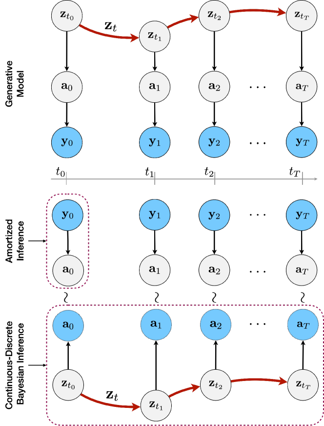
Figure 1: (Top) Generative model of Neural Continuous-Discrete State Space Model. The bold red arrows indicate that the state, ${\mathbf{z}}_{t}$, evolves continuously in time. The auxiliary variables, ${\mathbf{a}}_{k}$, and observations, ${\mathbf{y}}_{k}$, are emitted at arbitrary discrete timesteps $t_{k}\in\{t_{0},t_{1},\dots,t_{T}\}$. (Bottom) Amortized inference for auxiliary variables and continuous-discrete Bayesian inference for states. Samples from the amortized variational distribution over auxiliary variables are used as pseudo-observations to condition and perform inference in the continuous-discrete SSM at the bottom.

Recently, latent variable models based on neural differential equations have gained popularity for continuous-time modeling of time series (Chen et al., 2018; Rubanova et al., 2019; Yildiz et al., 2019; Li et al., 2020; Liu et al., 2020; Solin et al., 2021). However, these models suffer from limitations. The ordinary differential equation (ODE)-based models employ deterministic latent dynamics and/or encode the entire context window into an initial state, creating a restrictive bottleneck. Stochastic differential equation (SDE)-based models use stochastic latent dynamics, but typically perform a variational approximation of the latent trajectories via posterior SDEs. The posterior SDEs incorporate new observations in an ad-hoc manner, potentially resulting in a disparity between the posterior and generative transition dynamics, and a non-Markovian state space.

To address these issues, we propose the Neural Continuous-Discrete State Space Model (NCDSSM) that uses discrete-time observations to model continuous-time stochastic Markovian dynamics (Fig. 1). By using auxiliary variables, NCDSSM disentangles recognition of high-dimensional observations from dynamics (encoded by the state) (Fraccaro et al., 2017; Kurle et al., 2020). We leverage the rich literature on continuous-discrete filtering theory (Jazwinski, 1970), which has remained relatively underexplored in the modern deep learning context (Schirmer et al., 2022). Our proposed inference algorithm only performs amortized variational inference for the auxiliary variables since they enable classic continuous-discrete Bayesian inference (Jazwinski, 1970) for the states, using only the generative model. This obviates the need for posterior SDEs and allows incorporation of new observations via a principled Bayesian update, resulting in accurate state estimation. As a result, NCDSSM enables online prediction and naturally provides state uncertainty estimates. We propose three dynamics parameterizations for NCDSSM (linear time-invariant, non-linear and locally-linear) and a training objective that can be easily computed during inference.

We evaluated NCDSSM on imputation and forecasting tasks on multiple benchmark datasets. Our experiments demonstrate that NCDSSM accurately captures the underlying dynamics of the time series and extrapolates it consistently beyond the training context, significantly outperforming baseline models. From a practical perspective, we found that NCDSSM is less sensitive to random initializations and requires fewer parameters than the baselines.

In summary, the key contributions of this work are:

• NCDSSM, a continuous-discrete SSM with auxiliary variables for continuous-time modeling of irregularly-sampled (high dimensional) time series;

• An accurate inference algorithm that performs amortized inference for auxiliary variables and classic Bayesian inference for the dynamic states;

• An efficient learning algorithm and its stable implementation using square root factors;

• Experiments on multiple benchmark datasets, demonstrating that NCDSSM learns accurate models of the underlying dynamics and extrapolates it consistently into the future.

2 Approximate Continuous-Discrete Inference

We begin with a review of approximate continuous-discrete Bayesian filtering and smoothing, inference techniques employed by our proposed model. Consider the following Itô SDE,

$$d{\mathbf{z}}_{t}={\mathbf{f}}({\mathbf{z}}_{t},t)dt+{\mathbf{G}}({\mathbf{z}}_{t},t)d{\mathbf{B}}_{t},$$ (1)

where ${\mathbf{z}}_{t}\in\mathbb{R}^{m}$ is the state, ${\mathbf{B}}_{t}\in\mathbb{R}^{m}$ denotes a Brownian motion with diffusion matrix ${\mathbf{Q}}$, ${\mathbf{f}}(\cdot,t):\mathbb{R}^{m}\to\mathbb{R}^{m}$ is the drift function and ${\mathbf{G}}(\cdot,t):\mathbb{R}^{m}\to\mathbb{R}^{m\times m}$ is the diffusion function at time $t$. The initial density of the state, $p({\mathbf{z}}_{0})$, is assumed to be known and independent of the Brownian motion, ${\mathbf{B}}_{t}$. The evolution of the marginal density of the state, $p_{t}({\mathbf{z}}_{t})$, is governed by the Fokker-Plank-Kolmogorov (FPK) equation (Jazwinski, 1970, Ch. 4),

$$\frac{\partial p_{t}({\mathbf{z}}_{t})}{\partial t}=\mathscr{L}^{\ast}p_{t},$$ (2)

where $\mathscr{L}^{\ast}$ is the forward diffusion operator given by

$$\mathscr{L}^{\ast}\varphi=-\sum_{i=1}^{d}\frac{\partial}{\partial x_{i}}\left[\varphi f_{i}\right]+\frac{1}{2}\sum_{i=1}^{d}\sum_{j=1}^{d}\left[\varphi({\mathbf{G}}{\mathbf{Q}}{\mathbf{G}}^{\top})_{ij}\right].$$

In practice, we only have access to noisy transformations (called measurements or observations), ${\mathbf{a}}_{t_{k}}\in\mathbb{R}^{d}$, of the state, ${\mathbf{z}}_{t_{k}}$, at discrete timesteps $t_{k}\in\{t_{0},\dots,t_{T}\}$. In the following, we employ the notation ${\mathbf{x}}_{t}$ to represent the value of a variable ${\mathbf{x}}$ at an arbitrary continuous time $t$, and ${\mathbf{x}}_{t_{k}}$ (or ${\mathbf{x}}_{k}$ for short) to represent its value at the time $t_{k}$ associated with the $k$-th discrete timestep. The continuous-discrete state space model (Jazwinski, 1970, Ch. 6) is an elegant framework for modeling such time series.

Definition 2.1 (Continuous-Discrete State Space Model).

A continuous-discrete state space model is one where the latent state, ${\mathbf{z}}_{t}$, follows the continuous-time dynamics governed by Eq. (1) and the measurement, ${\mathbf{a}}_{k}$, at time $t_{k}$ is obtained from the measurement model $p({\mathbf{a}}_{k}|{\mathbf{z}}_{t_{k}})$.

In this work, we consider linear Gaussian measurement models, ${\mathbf{a}}_{k}\sim{\mathcal{N}}({\mathbf{a}}_{k};{\mathbf{H}}{\mathbf{z}}_{t_{k}},{\mathbf{R}}),$ where ${\mathbf{H}}\in\mathbb{R}^{d\times m}$ is the measurement matrix and ${\mathbf{R}}\succeq 0\in\mathbb{R}^{d\times d}$ is the measurement covariance matrix. Given observations ${\mathcal{A}}_{\tau}=\{{\mathbf{a}}_{k}:t_{k}\leq\tau\}$, we are interested in answering two types of inference queries: the posterior distribution of the state, ${\mathbf{z}}_{t}$, conditioned on observations up to time $t$, $p_{t}({\mathbf{z}}_{t}|{\mathcal{A}}_{t})$, and the posterior distribution of the state, ${\mathbf{z}}_{t}$, conditioned on all available observations, $p_{t}({\mathbf{z}}_{t}|{\mathcal{A}}_{T})$. These are known as the filtering and smoothing problems, respectively.

The filtering density, $p_{t}({\mathbf{z}}_{t}|{\mathcal{A}}_{t})$, satisfies the FPK equation (Eq. 2) for $t\in[t_{k},t_{k+1})$ between observations, with the initial condition $p_{t}({\mathbf{z}}_{t}|{\mathcal{A}}_{t_{k}})$ at time $t_{k}$. Observations can be incorporated via a Bayesian update,

$$p_{t}({\mathbf{z}}_{t_{k}}|{\mathcal{A}}_{t_{k}})=\frac{p({\mathbf{a}}_{t_{k}}|{\mathbf{z}}_{t_{k}})p({\mathbf{z}}_{t_{k}}|{\mathcal{A}}_{t_{k-1}})}{p({\mathbf{a}}_{k}|{\mathcal{A}}_{t_{k-1}})}.$$ (3)

The smoothing density satisfies a backward partial differential equation related to the FPK equation. We refer the reader to Anderson (1972) and Särkkä & Solin (2019, Ch. 10) for details and discuss a practical approximate filtering procedure in the following (cf. Appendix B.1 for smoothing).

2.1 Continuous-Discrete Bayesian Filtering

Solving Eq. (2) for arbitrary ${\mathbf{f}}$ and ${\mathbf{G}}$ is intractable; hence, several approximations have been considered in the literature (Särkkä & Solin, 2019, Ch. 9). The Gaussian assumed density approximation uses a Gaussian approximation,

$$p_{t}({\mathbf{z}}_{t})\approx{\mathcal{N}}({\mathbf{z}}_{t};{\mathbf{m}}_{t},{\mathbf{P}}_{t}),$$ (4)

for the solution to the FPK equation, characterized by the time-varying mean, ${\mathbf{m}}_{t}$, and covariance matrix, ${\mathbf{P}}_{t}$. Further, linearization of the drift ${\mathbf{f}}$ via Taylor expansion results in the following ODEs that govern the evolution of the mean and covariance matrix,

$$\frac{d{\mathbf{m}}_{t}}{dt} ={\mathbf{f}}({\mathbf{m}}_{t},t),$$ (5a)

$$\frac{d\mathbf{P}_{t}}{dt} ={\mathbf{F}}_{{\mathbf{z}}}({\mathbf{m}}_{t},t){\mathbf{P}}_{t}+{\mathbf{P}}_{t}{\mathbf{F}}^{\top}_{{\mathbf{z}}}({\mathbf{m}}_{t},t)+{\mathbf{D}}({\mathbf{m}}_{t},t),$$ (5b)

where ${\mathbf{F}}_{{\mathbf{z}}}({\mathbf{m}}_{t},t)$ is the Jacobian of ${\mathbf{f}}({\mathbf{z}},t)$ with respect to ${\mathbf{z}}$ at ${\mathbf{m}}_{t}$ and ${\mathbf{D}}(\cdot,t)={\mathbf{G}}(\cdot,t){\mathbf{Q}}{\mathbf{G}}^{\top}(\cdot,t)$. Thus, for $t\in[t_{k},t_{k+1})$ between observations, the filter distribution $p_{t}({\mathbf{z}}_{t}|{\mathcal{A}}_{t})$ can be approximated as a Gaussian with mean and covariance matrix given by solving Eq. (5), with initial conditions ${\mathbf{m}}_{t_{k}}$ and ${\mathbf{P}}_{t_{k}}$ at time $t_{k}$. This is known as the prediction step.

The Gaussian assumed density approximation of $p({\mathbf{z}}_{t_{k}}|{\mathcal{A}}_{t_{k-1}})$ described above makes the Bayesian update in Eq. (3) analytically tractable as $p({\mathbf{a}}_{t_{k}}|{\mathbf{z}}_{t_{k}})$ is also a Gaussian distribution with mean ${\mathbf{H}}{\mathbf{z}}_{k}$ and covariance matrix ${\mathbf{R}}$. The parameters, ${\mathbf{m}}_{k}$ and $\mathbf{P}_{k}$, of the Gaussian approximation of $p_{t}({\mathbf{z}}_{t_{k}}|{\mathcal{A}}_{t_{k}})$ are then given by,

$${\mathbf{S}}_{k} =\mathbf{H}\mathbf{P}_{k}^{-}\mathbf{H}^{\top}+\mathbf{R},$$ (6a)

$$\mathbf{K}_{k} =\mathbf{P}_{k}^{-}\mathbf{H}^{\top}{\mathbf{S}}_{k}^{-1},$$ (6b)

$${\mathbf{m}}_{k} ={\mathbf{m}}_{k}^{-}+\mathbf{K}_{k}\left({\mathbf{a}}_{k}-\mathbf{H}{\mathbf{m}}_{k}^{-}\right),$$ (6c)

$$\mathbf{P}_{k} =\mathbf{P}_{k}^{-}-\mathbf{K}_{k}{\mathbf{S}}_{k}\mathbf{K}^{\top}_{k},$$ (6d)

where ${\mathbf{m}}_{k}^{-}$ and $\mathbf{P}_{k}^{-}$ are the parameters of $p_{t}({\mathbf{z}}_{t_{k}}|{\mathcal{A}}_{t_{k-1}})$ given by the prediction step. Eq. (6) constitutes the update step which is exactly the same as the update step in the Kalman filter for discrete-time linear Gaussian SSMs. The continuous-time prediction step together with the discrete-time update step is sometimes also referred to as the hybrid Kalman filter. As a byproduct, the update step also provides the conditional likelihood terms, $p({\mathbf{a}}_{k}|{\mathcal{A}}_{t_{k-1}})={\mathcal{N}}({\mathbf{a}}_{k};\mathbf{H}{\mathbf{m}}_{k}^{-},{\mathbf{S}}_{k}),$ which can be combined to give the likelihood of the observed sequence, $p({\mathcal{A}}_{t_{T}})=p({\mathbf{y}}_{0})\prod_{k=1}^{T}p({\mathbf{a}}_{k}|{\mathcal{A}}_{t_{k-1}}).$

3 Neural Continuous-Discrete State Space Models

In this section, we describe our proposed model: Neural Continuous-Discrete State Space Model (NCDSSM). We begin by formulating NCDSSM as a continuous-discrete SSM with auxiliary variables that serve as succinct representations of high-dimensional observations. We then discuss how to perform efficient inference along with parameter learning and a stable implementation for NCDSSM.

3.1 Model Formulation

NCDSSM is a continuous-discrete SSM in which the latent state, ${\mathbf{z}}_{t}\in\mathbb{R}^{m}$, evolves in continuous time, emitting linear-Gaussian auxiliary variables, ${\mathbf{a}}_{t}\in\mathbb{R}^{h}$, which in turn emit observations, ${\mathbf{y}}_{t}\in\mathbb{R}^{d}$. Thus, NCDSSM possesses two types of latent variables: (a) the states that encode the hidden dynamics, and (b) the auxiliary variables that can be viewed as succinct representations of the observations and are equivalent to observations in the continuous-discrete state space models considered in Section 2. The inclusion of auxiliary variables offers two benefits; (i) it allows disentangling representation learning (or recognition) from dynamics (encoded by ${\mathbf{z}}_{t}$) and (ii) it enables the use of arbitrary decoders to model the conditional distribution $p({\mathbf{y}}_{t}|{\mathbf{a}}_{t})$. We discuss this further in Section 3.2.

Consider the case when we have observations available at discrete timesteps $t_{0},\dots,t_{T}$. Following the graphical model in Fig. 1, the joint distribution over the states ${\mathbf{z}}_{0:T}$, the auxiliary variables ${\mathbf{a}}_{0:T}$, and the observations ${\mathbf{y}}_{0:T}$ factorises as

$$p_{\theta}({\mathbf{z}}_{0:T}, {\mathbf{a}}_{0:T},{\mathbf{y}}_{0:T})=\prod_{k=0}^{T}p({\mathbf{y}}_{k}|{\mathbf{a}}_{k})p({\mathbf{a}}_{k}|{\mathbf{z}}_{k})p({\mathbf{z}}_{k}|{\mathbf{z}}_{{k-1}}),$$

where ${\mathbf{x}}_{0:T}$ denotes the set $\{{\mathbf{x}}_{t_{0}},\dots,{\mathbf{x}}_{t_{T}}\}$ and $p({\mathbf{z}}_{0}|{\mathbf{z}}_{{-1}})=p({\mathbf{z}}_{0})$. We model the initial (prior) distribution of the states as a multivariate Gaussian distribution,

$$p({\mathbf{z}}_{0})={\mathcal{N}}({\mathbf{z}}_{0};\bm{\mu}_{0},\bm{\Sigma}_{0}),$$ (7)

where $\bm{\mu}_{0}\in\mathbb{R}^{m}$ and $\bm{\Sigma}_{0}\succeq 0\in\mathbb{R}^{m\times m}$ are the mean and covariance matrix, respectively. The transition distribution of the states, $p({\mathbf{z}}_{k}|{\mathbf{z}}_{{k-1}})$, follows the dynamics governed by the SDE in Eq. (1). The conditional emission distributions of the auxiliary variables and observations are modeled as multivariate Gaussian distributions given by,

$$p({\mathbf{a}}_{k}|{\mathbf{z}}_{k}) ={\mathcal{N}}({\mathbf{a}}_{k};\mathbf{H}{\mathbf{z}}_{k},{\mathbf{R}}),$$ (8)

$$p({\mathbf{y}}_{k}|{\mathbf{a}}_{k}) ={\mathcal{N}}({\mathbf{y}}_{k};f^{\mu}({\mathbf{a}}_{k}),f^{\Sigma}({\mathbf{a}}_{k})),$$ (9)

where ${\mathbf{H}}~{}\in~{}\mathbb{R}^{h\times m}$ is the auxiliary measurement matrix, ${\mathbf{R}}~{}\succeq~{}0~{}\in~{}\mathbb{R}^{h\times h}$ is the auxiliary covariance matrix, and $f^{\mu}$ and $f^{\Sigma}$ are functions parameterized by neural networks that output the mean and the covariance matrix of the distribution, respectively. We use $\theta$ to denote the parameters of the generative model, including SSM parameters $\{\bm{\mu}_{0},\bm{\Sigma}_{0},{\mathbf{f}},{\mathbf{Q}},{\mathbf{G}},{\mathbf{H}},{\mathbf{R}}\}$ and observation emission distribution parameters $\{f^{\mu},f^{\Sigma}\}$.

We propose three variants of NCDSSM, depending on the parameterization of ${\mathbf{f}}$ and ${\mathbf{G}}$ functions in Eq. (1) that govern the dynamics of the state:

Linear time-invariant dynamics is obtained by parameterizing ${\mathbf{f}}$ and ${\mathbf{G}}$ as

$${\mathbf{f}}({\mathbf{z}}_{t},t)={\mathbf{F}}{\mathbf{z}}_{t}\quad\text{and}\quad{\mathbf{G}}({\mathbf{z}},t)={\mathbf{I}},$$ (10)

respectively, where ${\mathbf{F}}\in\mathbb{R}^{m\times m}$ is a Markov transition matrix and ${\mathbf{I}}$ is the $m$-dimensional identity matrix. In this case, Eqs. (4) and (5) become exact and the ODEs in Eq. (5) can be solved analytically using matrix exponentials (cf. Appendix B.2). Unfortunately, the restriction of linear dynamics is limiting for practical applications. We denote this linear time-invariant variant as NCDSSM-LTI.

Non-linear dynamics is obtained by parameterizing ${\mathbf{f}}$ and ${\mathbf{G}}$ using neural networks. With sufficiently powerful neural networks, this parameterization is flexible enough to model arbitrary non-linear dynamics. However, the neural networks need to be carefully regularized (cf. Appendix LABEL:app:stable-implementation) to ensure optimization and inference stability. Inference in this variant also requires computation of the Jacobian of a neural network for solving Eq. (5). We denote this non-linear variant as NCDSSM-NL.

Locally-linear dynamics is obtained by parameterizing ${\mathbf{f}}$ and ${\mathbf{G}}$ as

$${\mathbf{f}}({\mathbf{z}}_{t},t)={\mathbf{F}}({\mathbf{z}}_{t}){\mathbf{z}}_{t}\quad\text{and}\quad{\mathbf{G}}({\mathbf{z}},t)={\mathbf{I}},$$ (11)

respectively, where the matrix ${\mathbf{F}}({\mathbf{z}}_{t})\in\mathbb{R}^{m\times m}$ is given by a convex combination of $K$ base matrices $\{{\mathbf{F}}^{(j)}\}_{j=1}^{K}$,

$${\mathbf{F}}({\mathbf{z}}_{t})=\sum_{j=1}^{K}\alpha^{(j)}({\mathbf{z}}_{t}){\mathbf{F}}^{(j)},$$ (12)

and the combination weights, $\alpha({\mathbf{z}}_{t})$, are given by

$$\alpha({\mathbf{z}}_{t})=\mathrm{softmax}(g({\mathbf{z}}_{t})),$$ (13)

where $g$ is a neural network. Such parameterizations smoothly interpolate between linear SSMs and can be viewed as “soft” switching SSMs. Locally-linear dynamics has previously been used for discrete-time SSMs (Karl et al., 2016; Klushyn et al., 2021); we extend it to the continuous time setting by evaluating Eq. (12) continuously in time. Unlike non-linear dynamics, this parameterization does not require careful regularization and its flexibility can be controlled by choosing the number of base matrices, $K$. Furthermore, the Jacobian of ${\mathbf{f}}$ in Eq. (5) can be approximated as ${\mathbf{F}}({\mathbf{m}}_{t})$, avoiding the expensive computation of the Jacobian of a neural network (Klushyn et al., 2021). We denote this locally-linear variant as NCDSSM-LL.

3.2 Inference

Exact inference in the model described above is intractable when the dynamics is non-linear and/or the observation emission distribution, $p({\mathbf{y}}_{k}|{\mathbf{a}}_{k})$, is modeled by arbitrary non-linear functions. In the modern deep learning context, a straightforward approach would be to approximate the posterior distribution over the states and auxiliary variables, $q({\mathbf{z}}_{0:T},{\mathbf{a}}_{0:T}|{\mathbf{y}}_{0:T})$, using recurrent neural networks (e.g., using ODE-RNNs when modeling in continuous time). However, such parameterizations have been shown to lead to poor optimization of the transition model in discrete-time SSMs, leading to inaccurate learning of system dynamics (Klushyn et al., 2021). Alternatively, directly applying continuous-discrete inference techniques to non-linear emission models requires computation of Jacobian matrices and inverses of $d\times d$ matrices (cf. Eq. 6) which scales poorly with the data dimensionality.

The introduction of linear-Gaussian auxiliary variables offers a middle ground between the two options above. It allows efficient use of continuous-discrete Bayesian inference techniques for the inference of states, avoiding fully amortized inference for auxiliary variables and states. Concretely, we split our inference procedure into two inference steps: (i) for auxiliary variables and (ii) for states.

Inference for auxiliary variables.

We perform amortized inference for the auxiliary variables, factorizing the variational distribution as,

$$q_{\phi}({\mathbf{a}}_{0:T}|{\mathbf{y}}_{0:T})=\prod_{k=0}^{T}q({\mathbf{a}}_{k}|{\mathbf{y}}_{k}),$$ (14)

where $q({\mathbf{a}}_{k}|{\mathbf{y}}_{k})={\mathcal{N}}({\mathbf{a}}_{k};f_{\phi}^{\mu}({\mathbf{y}}_{k}),f_{\phi}^{\Sigma}({\mathbf{y}}_{k}))$ and $f_{\phi}^{\mu}$, $f_{\phi}^{\Sigma}$ are neural networks. This can be viewed as the recognition network in a variational autoencoder, per timestep. This flexible factorization permits use of arbitrary recognition networks, thereby allowing arbitrary non-linear emission distributions, $p({\mathbf{y}}_{k}|{\mathbf{a}}_{k})$.

Inference for states.

Given the variational distribution $q_{\phi}({\mathbf{a}}_{0:T}|{\mathbf{y}}_{0:T})$ in Eq. (14), we can draw samples, $\tilde{{\mathbf{a}}}_{0:T}\sim q_{\phi}({\mathbf{a}}_{0:T}|{\mathbf{y}}_{0:T})$, from it. Viewing $\tilde{{\mathbf{a}}}_{0:T}$ as pseudo-observations, we treat the remaining SSM (i.e., the states and auxiliary variables) separately. Specifically, conditioned on the auxiliary variables, $\tilde{{\mathcal{A}}}_{\tau}=\{\tilde{{\mathbf{a}}}_{k}:t_{k}\leq\tau\}$, we can answer inference queries over the states ${\mathbf{z}}_{t}$ in continuous time. This does not require additional inference networks and can be performed only using the generative model via classic continuous-discrete Bayesian inference techniques in Section 2. To infer the filtered density, $p_{t}({\mathbf{z}}_{t}|\tilde{{\mathcal{A}}}_{t})$, we can use Eq. (5) for the prediction step and Eq. (6) for the update step, replacing ${\mathbf{y}}_{k}$ by $\tilde{{\mathbf{a}}}_{k}$. Similarly, we can use Eq. (23) (Appendix) to infer the smoothed density, $p_{t}({\mathbf{z}}_{t}|\tilde{{\mathcal{A}}}_{T})$.

As the inference of states is now conditioned on auxiliary variables, only the inversion of $h\times h$ matrices is required which is computationally feasible as ${\mathbf{a}}_{k}$ generally has lower dimensionality than ${\mathbf{y}}_{k}$. Notably, this inference scheme does not require posterior SDEs for inference (as in other SDE-based models; cf. Section 4) and does not suffer from poor optimization of the transition model as we employ the (generative) transition model for the inference of states.

3.3 Learning

The parameters of the generative model $\{\theta\}$ and the inference network $\{\phi\}$ can be jointly optimized by maximizing the following evidence lower bound (ELBO) of the log-likelihood, $\log p_{\theta}({\mathbf{y}}_{0:T})$,

$$\log p_{\theta}({\mathbf{y}}_{0:T})$$

$$\>\geq\mathbb{E}_{q_{\phi}({\mathbf{a}}_{0:T}|{\mathbf{y}}_{0:T})}\left[\log\frac{\prod_{k=0}^{T}p_{\theta}({\mathbf{y}}_{k}|{\mathbf{a}}_{k})p_{\theta}({\mathbf{a}}_{0:T})}{\prod_{k=0}^{T}q_{\phi}({\mathbf{a}}_{k}|{\mathbf{y}}_{k})}\right]$$

$$\>=:{\mathcal{L}}_{\mathrm{ELBO}}(\theta,\phi).$$ (15)

The distributions $p_{\theta}({\mathbf{y}}_{k}|{\mathbf{a}}_{k})$ and $q_{\phi}({\mathbf{a}}_{k}|{\mathbf{y}}_{k})$ in ${\mathcal{L}}_{\mathrm{ELBO}}$ are immediately available via the emission and recognition networks, respectively. What remains is the computation of $p_{\theta}({\mathbf{a}}_{0:T})$. Fortunately, $p_{\theta}({\mathbf{a}}_{0:T})$ can be computed as a byproduct of the inference (filtering) procedure described in Section 3.2. The distribution factorizes as

$$p({\mathbf{a}}_{0:T})=p({\mathbf{a}}_{0})\prod_{k=1}^{T}p({\mathbf{a}}_{k}|{\mathcal{A}}_{t_{k-1}}),$$

where $p({\mathbf{a}}_{k}|{\mathcal{A}}_{t_{k-1}})={\mathcal{N}}({\mathbf{a}}_{k};\mathbf{H}{\mathbf{m}}_{k}^{-},{\mathbf{S}}_{k})$, and ${\mathbf{m}}_{k}^{-}$ and ${\mathbf{S}}_{k}$ are computed during the prediction and update steps, respectively. The $p_{\theta}({\mathbf{a}}_{0:T})$ term can be viewed as a “prior” over the auxiliary variables. However, unlike the fixed standard Gaussian prior in a vanilla variational autoencoder, $p_{\theta}({\mathbf{a}}_{0:T})$ is a learned prior given by the marginalization of the states, ${\mathbf{z}}_{t}$, from the underlying SSM. Algorithm 1 summarizes the learning algorithm for a single time series; in practice, mini-batches of time series are sampled from the dataset.

Algorithm 1 Learning in Neural Continuous-Discrete State Space Models

Observations $\{({\mathbf{y}}_{k},t_{k})\}_{k=0}^{T}$and model parameters $\{\theta,\phi\}$. Compute $q_{\phi}({\mathbf{a}}_{0:T}|{\mathbf{y}}_{0:T})$using Eq. (). Sample $\tilde{{\mathbf{a}}}_{0:T}\sim q_{\phi}({\mathbf{a}}_{0:T}|{\mathbf{y}}_{0:T})$. $\underline{\hskip 10.00002pt},\log p_{\theta}(\tilde{{\mathbf{a}}}_{0:T})\leftarrow$Filter$\tilde{{\mathbf{a}}}_{0:T}$, $t_{0:T}$; $\theta$$\triangleright$cf. Algorithm 3(Appendix) for Filter. Compute $\prod_{k=0}^{T}p_{\theta}({\mathbf{y}}_{k}|\tilde{{\mathbf{a}}}_{k})$using Eq. (). Optimize ${\mathcal{L}}_{\mathrm{ELBO}}(\theta,\phi)$. end of training.

3.4 Stable Implementation

A naive implementation of the numerical integration of ODEs (Eqs. 5 and 23) and other operations (Eq. 6) results in unstable training and crashing due to violation of the positive definite constraint for the covariance matrices. Commonly employed tricks such as symmetrization, ${\mathbf{P}}=({\mathbf{P}}+{\mathbf{P}}^{\top})/2,$ and addition of a small positive number ($\epsilon$) to the diagonal elements, ${\mathbf{P}}={\mathbf{P}}+\epsilon{\mathbf{I}},$ did not solve these training issues. Therefore, we implemented our algorithms in terms of square root (Cholesky) factors, which proved critical to the stable training of NCDSSM. Several square root factors’ based inference algorithms have been previously proposed (Zonov, 2019; Jorgensen et al., 2007; Kailath et al., 2000, Ch. 12). In the following, we discuss our implementation which is based on Zonov (2019). Further discussion on implementation stability, particularly in the case of non-linear dynamics, can be found in Appendix LABEL:app:stable-implementation.

We begin with a lemma that shows that the square root factor of the sum of two matrices with square root factors can be computed using $\mathrm{QR}$ decomposition.

Lemma 3.1.

Let ${\mathbf{A}}$ and ${\mathbf{B}}$ be two $n\times n$ matrices with square root factors ${\mathbf{A}}^{1/2}$ and ${\mathbf{B}}^{1/2}$, respectively. The matrix ${\mathbf{C}}={\mathbf{A}}+{\mathbf{B}}$ also has a square root factor, ${\mathbf{C}}^{1/2}$, given by

$$\Theta,\begin{bmatrix}{\mathbf{C}}^{1/2}&\mathbf{0}_{n\times n}\end{bmatrix}^{\top}=\mathrm{QR}\left(\begin{bmatrix}{\mathbf{A}}^{1/2}&{\mathbf{B}}^{1/2}\end{bmatrix}^{\top}\right),$$

where $\Theta$ is the orthogonal $\mathrm{Q}$ matrix given by $\mathrm{QR}$ decomposition and $\mathbf{0}_{n\times n}$ is an $n\times n$ matrix of zeros.

Prediction step.

The solution of matrix differential equations of the form in Eq. (5b) — called Lyapunov differential equations — over $[t_{0},t_{1}]$ is given by (Abou-Kandil et al., 2012, Corollary 1.1.6)

$${\mathbf{P}}_{t_{1}}=\bm{\Phi}_{t_{1}}{\mathbf{P}}_{t_{0}}\bm{\Phi}_{t_{1}}^{\top}+\int_{t_{0}}^{t_{1}}\bm{\Phi}_{t}{\mathbf{D}}_{t}\bm{\Phi}_{t}^{\top}dt,$$ (16)

where $\bm{\Phi}_{t}$, called the fundamental matrix, is defined by

$$\frac{d\bm{\Phi}_{t}}{dt}={\mathbf{F}}_{{\mathbf{z}}}({\mathbf{m}}_{t},t)\bm{\Phi}_{t}\>\>\text{and}\>\>\bm{\Phi}_{t_{0}}={\mathbf{I}}.$$ (17)

This initial value problem can be solved using an off-the-shelf ODE solver. Let $\{\tilde{\bm{\Phi}}_{1}={\mathbf{I}},\tilde{\bm{\Phi}}_{2},\dots,\tilde{\bm{\Phi}}_{n}\}$ be intermediate solutions of Eq. (17) given by an ODE solver with step size $\eta$, Eq. (16) can be approximated as

$${\mathbf{P}}_{t_{1}} \approx\tilde{\bm{\Phi}}_{n}{\mathbf{P}}_{t_{0}}\tilde{\bm{\Phi}}_{n}^{\top}$$

$$+\frac{\eta}{2}\left(\tilde{\bm{\Phi}}_{1}{\mathbf{D}}_{1}\tilde{\bm{\Phi}}_{1}^{\top}+2\tilde{\bm{\Phi}}_{2}{\mathbf{D}}_{2}\tilde{\bm{\Phi}}_{2}^{\top}+\dots+\tilde{\bm{\Phi}}_{n}{\mathbf{D}}_{n}\tilde{\bm{\Phi}}_{n}^{\top}\right).$$ (18)

The additions in Eq. (18) are performed using Lemma 3.1 with square root factors $\tilde{\bm{\Phi}}_{n}{\mathbf{P}}_{t_{0}}^{1/2}$ and $\{\tilde{\bm{\Phi}}_{j}{\mathbf{D}}_{j}^{1/2}\}_{j=1}^{n}$.

Update step.

Using similar arguments as in the proof of Lemma 3.1 (cf. Appendix LABEL:app:stable-implementation for details), the update step (Eq. 6) can be performed by the $\mathrm{QR}$ decomposition of the square root factor

$$\begin{bmatrix}{\mathbf{R}}^{1/2}&{\mathbf{H}}({\mathbf{P}}_{k}^{-})^{1/2}\\ \mathbf{0}_{m\times d}&({\mathbf{P}}_{k}^{-})^{1/2}\end{bmatrix}^{\top}.$$ (19)

Let $\begin{bmatrix}{\mathbf{X}}&\mathbf{0}\\ {\mathbf{Y}}&{\mathbf{Z}}\end{bmatrix}^{\top}$ be the upper triangular $\mathrm{R}$ matrix obtained from the $\mathrm{QR}$ decomposition of (19). The square root factor of the updated covariance matrix, ${\mathbf{P}}_{k}^{1/2}$, and the Kalman gain matrix, ${\mathbf{K}}_{k}$, are then given by ${\mathbf{P}}_{k}^{1/2}={\mathbf{Z}}$ and ${\mathbf{K}}_{k}={\mathbf{Y}}{\mathbf{X}}^{-1}$, respectively.

4 Related Work

ODE-based models.

Since the introduction of the NeuralODE (Chen et al., 2018), various models based on neural ODEs have been proposed for continuous-time modeling of time series. LatentODE (Rubanova et al., 2019) encodes the entire context window into an initial state using an encoder (e.g., ODE-RNN) and uses a NeuralODE to model the latent dynamics. ODE2VAE (Yildiz et al., 2019) decomposes the latent state into position and velocity components to explicitly model the acceleration and parameterize the ODE dynamics with Bayesian neural networks, thus accommodating uncertainty. Nevertheless, both models lack a mechanism to update the latent state based on new observations. To address this limitation, NeuralCDE (Kidger et al., 2020) incorporates techniques from rough path theory to control the latent state using observations. Conversely, GRU-ODE-B (De Brouwer et al., 2019) and NJ-ODE (Herrera et al., 2020) combine neural ODEs with a Bayesian-inspired update step, enabling the incorporation of new observations. Unlike prior models, NCDSSM incorporates observations via a principled Bayesian update and disentangles recognition from dynamics using auxiliary variables.

SDE-based models.

LatentSDE (Li et al., 2020) uses a posterior SDE in the latent space to infer the latent dynamics together with a prior (generative) SDE in a variational setup. Solin et al. (2021) proposed a variant of LatentSDE trained by exploiting the Gaussian assumed density approximation of the non-linear SDE. VSDN (Liu et al., 2020) uses ODE-RNNs to provide historical information about the time series to the SDE drift and diffusion functions. These models rely on posterior SDEs to infer the dynamics, and new observations are incorporated in an ad-hoc manner. This approach can potentially lead to discrepancies between the posterior and generative dynamics, as well as non-Markovian state spaces. In contrast, NCDSSM employs stochastic Markovian dynamics, incorporates observations through principled Bayesian updates, and performs continuous-discrete Bayesian inference for the state variables (dynamics), eliminating the need for posterior SDEs.

State space models.

Several prior works (Chung et al., 2015; Krishnan et al., 2015; Karl et al., 2016; Krishnan et al., 2017; Doerr et al., 2018) have proposed SSM-like models for discrete-time sequential data, trained via amortized variational inference. Unlike NCDSSM, these models approximate sequential Bayesian inference (i.e., filtering and smoothing) via deterministic RNNs and are limited to the discrete time setting. More recently, deterministic linear SSMs (Gu et al., 2021; Zhang et al., 2023), featuring specific transition matrices (Gu et al., 2020), have been introduced as components for sequence modeling. In contrast, our work proposes a general probabilistic continuous-discrete SSM that supports locally-linear and non-linear dynamics.

The combination of Bayesian inference for a subset of latent variables and amortized inference for others has been previously explored in SSMs. SNLDS (Dong et al., 2020) and REDSDS (Ansari et al., 2021) perform amortized inference for the states and exact inference for discrete random variables (switches and duration counts) in switching SSMs. KVAE (Fraccaro et al., 2017), EKVAE (Klushyn et al., 2021) and ARSGLS (Kurle et al., 2020) introduce auxiliary variables and perform classic Bayesian filtering and smoothing for the state variables, similar to NCDSSM. However, these models utilize specific parameterizations of state dynamics and operate on discrete-time sequential data. On the other hand, our proposed framework presents a general approach for continuous-time modeling of irregularly-sampled time series, allowing for multiple possible parameterizations of the dynamics.

The continuous recurrent unit (CRU) (Schirmer et al., 2022) is the most closely related model to NCDSSM, as it also employs continuous-discrete inference. However, there are notable distinctions between CRU and our work: (i) we propose a general framework offering multiple possible parameterizations of dynamics, while CRU focuses on specific locally-linear dynamics that are time-invariant between observed timesteps, unlike NCDSSM-LL, (ii) NCDSSM serves as an unconditional generative model, which fundamentally differs from CRU’s conditional training for downstream tasks, and (iii) NCDSSM utilizes continuous-time smoothing for imputation by incorporating future information through the backward (smoothing) pass, whereas CRU solely relies on the forward (filtering) pass.

5 Experiments

In this section, we present empirical results on time series imputation and forecasting tasks. Our primary focus was to investigate the models’ ability to capture the underlying dynamics of the time series, gauged by the accuracy of long-term forecasts beyond the training context. We experimented with the three variants of our model described in Section 3.1: NCDSSM-LTI, NCDSSM-NL, and NCDSSM-LL. Our main baselines were LatentODE and LatentSDE, two popular continuous-time latent variable models with deterministic and stochastic dynamics, respectively. We also compared NCDSSM against several other baselines for individual experiments. We first discuss experiment results on the low-dimensional bouncing ball and damped pendulum datasets, then move to higher dimensional settings: walking sequences from the CMU Motion Capture (MoCap) dataset, the USHCN daily climate dataset, and two 32x32 dimensional video datasets (Box and Pong). Our code is available at https://github.com/clear-nus/NCDSSM.

Table 1: Imputation and forecasting results for bouncing ball and damped pendulum datasets averaged over 50 sample trajectories. Mean ± standard deviation are computed over 5 independent runs.

Dataset	Model	Imputation MSE ($\downarrow$) (% Missing)			Forecast MSE ($\downarrow$) (% Missing)
		30%	50%	80%	0%	30%	50%	80%
Bouncing Ball	LatentODE (Rubanova et al., 2019)	0.007 ± 0.000	0.008 ± 0.001	0.011 ± 0.000	0.386 ± 0.025	0.489 ± 0.133	0.422 ± 0.053	0.412 ± 0.048
	LatentSDE (Li et al., 2020)	0.006 ± 0.000	0.007 ± 0.000	0.011 ± 0.001	0.408 ± 0.043	1.209 ± 1.115	1.567 ± 2.263	0.352 ± 0.077
	GRUODE-B (De Brouwer et al., 2019)	0.017 ± 0.001	0.026 ± 0.010	0.051 ± 0.003	0.868 ± 0.103	0.805 ± 0.315	0.856 ± 0.394	0.445 ± 0.182
	NCDSSM-LTI	0.020 ± 0.001	0.026 ± 0.001	0.067 ± 0.002	0.592 ± 0.106	0.557 ± 0.014	0.556 ± 0.025	0.555 ± 0.022
	NCDSSM-NL	0.006 ± 0.000	0.006 ± 0.000	0.007 ± 0.000	0.037 ± 0.018	0.036 ± 0.007	0.041 ± 0.007	0.115 ± 0.029
	NCDSSM-LL	0.006 ± 0.000	0.006 ± 0.000	0.008 ± 0.001	0.037 ± 0.028	0.034 ± 0.016	0.049 ± 0.034	0.076 ± 0.017
Damped Pendulum	LatentODE (Rubanova et al., 2019)	0.151 ± 0.002	0.155 ± 0.002	0.206 ± 0.013	0.097 ± 0.042	0.117 ± 0.001	0.119 ± 0.001	0.148 ± 0.007
	LatentSDE (Li et al., 2020)	0.092 ± 0.076	0.148 ± 0.001	0.229 ± 0.001	0.046 ± 0.046	0.084 ± 0.058	0.147 ± 0.020	0.357 ± 0.096
	GRUODE-B (De Brouwer et al., 2019)	0.015 ± 0.001	0.023 ± 0.003	0.064 ± 0.003	0.244 ± 0.107	0.424 ± 0.617	0.124 ± 0.088	0.037 ± 0.036
	NCDSSM-LTI	0.036 ± 0.001	0.057 ± 0.001	0.120 ± 0.002	0.282 ± 0.084	1.017 ± 1.363	1.527 ± 1.440	0.231 ± 0.050
	NCDSSM-NL	0.008 ± 0.000	0.011 ± 0.000	0.033 ± 0.002	0.011 ± 0.004	0.011 ± 0.003	0.012 ± 0.003	0.034 ± 0.019
	NCDSSM-LL	0.008 ± 0.000	0.011 ± 0.000	0.037 ± 0.003	0.025 ± 0.030	0.010 ± 0.001	0.020 ± 0.008	0.055 ± 0.007

5.1 Bouncing Ball and Damped Pendulum

The bouncing ball and damped pendulum datasets have known ground truth dynamics, which facilitates quality assessment of the dynamics learned by a given model. For details on these datasets, please refer to Appendix LABEL:app:datasets. In brief, the univariate bouncing ball dataset exhibits piecewise-linear dynamics, whilst bivariate damped pendulum dataset (Karl et al., 2016; Kurle et al., 2020) exhibits non-linear latent dynamics.

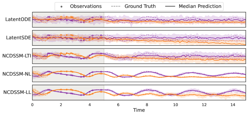
Figure 2: Predictions from different models on the damped pendulum dataset in the 80% missing data setting. The ground truth is shown using dashed lines with observed points in the context window (gray shaded region) shown as filled circles. The vertical dashed gray line marks the beginning of the forecast horizon. Solid lines indicate median predictions with 90% prediction intervals shaded around them. The purple and orange colors indicate observation dimensions. NCDSSM-NL and NCDSSM-LL are significantly better at forecasting compared to the baselines.

Table 2: Forecasting results for the CMU MoCap walking dataset averaged over 50 sample trajectories with 95% prediction interval based on the $t$-statistic in parentheses. ${}^{\dagger}$Baseline results from Solin et al. (2021).

Model	MSE ($\downarrow$)
	${}^{\dagger}$Setup 1	Setup 2
npODE (Heinonen et al., 2018)	22.96	–
NeuralODE (Chen et al., 2018)	22.49 (0.88)	–
ODE2VAE-KL (Yildiz et al., 2019)	8.09 (1.95)	–
LatentODE (Rubanova et al., 2019)	5.98 (0.28)	31.62 (0.05)
LatentSDE (Li et al., 2020)	4.03 (0.20)	9.52 (0.21)
LatentApproxSDE (Solin et al., 2021)	7.55 (0.05)	–
NCDSSM-LTI	13.90 (0.02)	5.22 (0.02)
NCDSSM-NL	5.69 (0.01)	6.73 (0.02)
NCDSSM-LL	9.96 (0.01)	4.74 (0.01)

We trained all the models on 10s/5s sequences (with a discretization of 0.1s) for bouncing ball/damped pendulum with 0%, 30%, 50% and 80% timesteps missing at random to simulate irregularly-sampled data. The models were evaluated on imputation of the missing timesteps and forecasts of 20s/10s beyond the training regime for bouncing ball/damped pendulum.

Table 1 reports the imputation and forecast mean squared error (MSE) for different missing data settings. In summary, the NCDSSM models with non-linear and locally-linear dynamics (NCDSSM-NL and NCDSSM-LL) perform well across datasets, settings, and random initializations, significantly outperforming the baselines. Furthermore, for these low-dimensional datasets, learning latent representations in the form of auxiliary variables is not required and we can set the recognition and emission functions in Eq. (14) and Eq. (9) to identity functions. This results in NCDSSM models requiring 2-5 times fewer parameters than LatentODE and LatentSDE (cf. Table LABEL:tab:parameter-comparison in the Appendix).

Fig. 2 shows example predictions from the best performing run of every model for 80% missing data for the pendulum (cf. Appendix LABEL:app:additional-results for other settings). NCDSSM-NL and NCDSSM-LL generates far better predictions both inside and outside the context window compared to the baselines. Ordinary least squares (OLS) goodness-of-fit results in Table LABEL:tab:ols-pendulum (Appendix) suggest that this performance can be attributed to our models having learnt the correct dynamics; latent states from NCDSSM-NL and NCDSSM-LL are highly correlated with the ground truth angle and angular velocity for all missingness scenarios. In other words, the models have learnt a Markovian state space which is informative about the dynamics at a specific time.

5.2 CMU Motion Capture (Walking)

This dataset comprises walking sequences of subject 35 from the CMU MoCap database containing joint angles of subjects performing everyday activities. We used a preprocessed version of the dataset from Yildiz et al. (2019) that has 23 50-dimensional sequences of length 300.

We tested the models under two setups. Setup 1  (Yildiz et al., 2019; Li et al., 2020; Solin et al., 2021) involves training on complete 300 timestep sequences from the training set and using only the first 3 timesteps as context to predict the remaining 297 timesteps during test time. Although challenging, this setup does not evaluate the model’s performance beyond the training context. Thus, we propose Setup 2 in which we train the model only using the first 200 timesteps. During test time, we give the first 100 timesteps as context and predict the remaining 200 timesteps.

The forecast MSE results for both setups are reported in Table 2. NCDSSM-NL performs better than all baselines except LatentSDE on Setup 1 while NCDSSM models perform significantly better than baselines on Setup 2. This showcases NCDSSM’s ability to correctly model the latent dynamics, aiding accurate long-term predictions beyond the training context.

5.3 USHCN Climate Indicators

We evaluated the models on the United States Historical Climatology Network (USHCN) dataset that comprises measurements of five climate indicators across the United States. The preprocessed version of this dataset from De Brouwer et al. (2019) contains sporadic time series (i.e., with measurements missing both over the time and feature axes) from 1,114 meteorological stations over 4 years. Following De Brouwer et al. (2019), we trained the models on sequences from the training stations and evaluated them on the task of predicting the next 3 measurements given the first 3 years as context from the held-out test stations. The results in Table 3 show that NCDSSM-NL outperforms all the baselines with NCDSSM-LTI and NCDSSM-LL performing better than most of the baselines.

5.4 Pymunk Physical Environments

Finally, we evaluated the models on two high-dimensional (video) datasets of physical environments used in Fraccaro et al. (2017), simulated using the Pymunk Physics engine (Blomqvist, 2022): Box and Pong. The box dataset consists of videos of a ball moving in a 2-dimensional box and the pong dataset consists of videos of a Pong-like environment where two paddles move to keep a ball in the frame at all times. Each frame is a 32x32 binary image.

Figure 3: Sample predictions from NCDSSM-NL on the Pong dataset. The top row is the ground truth with some missing observations in the context window. The next two rows show trajectories sampled from NCDSSM-NL upto 20 forecast steps. NCDSSM-NL is able to both impute and forecast accurately. Best viewed zoomed-in on a computer. More examples in Appendix LABEL:app:additional-results.

Table 3: Forecasting results for the USHCN climate dataset. Mean ± standard deviation are computed over 5 folds as described in De Brouwer et al. (2019). ${}^{\dagger}$Results from De Brouwer et al. (2019). ${}^{\ddagger}$Results from Liu et al. (2020).

Model	MSE ($\downarrow$)
${}^{\dagger}$NeuralODE-VAE (Chen et al., 2018)	0.83 ± 0.10
${}^{\dagger}$SequentialVAE (Krishnan et al., 2015)	0.83 ± 0.07
${}^{\dagger}$GRU-D (Che et al., 2018)	0.53 ± 0.06
${}^{\dagger}$T-LSTM (Baytas et al., 2017)	0.59 ± 0.11
${}^{\dagger}$GRUODE-B (De Brouwer et al., 2019)	0.43 ± 0.07
${}^{\ddagger}$ODE-RNN (Rubanova et al., 2019)	0.39 ± 0.06
${}^{\ddagger}$LatentODE (Rubanova et al., 2019)	0.77 ± 0.09
${}^{\ddagger}$LatentSDE (Li et al., 2020)	0.74 ± 0.11
${}^{\ddagger}$VSDN-F (IWAE) (Liu et al., 2020)	0.37 ± 0.06
NCDSSM-LTI	0.38 ± 0.07
NCDSSM-NL	0.34 ± 0.06
NCDSSM-LL	0.37 ± 0.06

Table 4: Forecasting results for the Box and Pong datasets averaged over 16 sample trajectories.

Model	EMD ($\downarrow$)
	Box	Pong
LatentODE (Rubanova et al., 2019)	1.792	4.543
LatentSDE (Li et al., 2020)	1.925	3.505
NCDSSM-LTI	1.685	3.265
NCDSSM-NL	0.692	1.714
NCDSSM-LL	0.632	1.891

We trained the models on sequences of 20 frames with 20% of these frames randomly dropped. At test time, the models were evaluated on forecasts of 40 frames beyond the training context. For evaluation, we treat each image as a probability distribution on the XY-plane and report the earth mover’s distance (EMD) between the ground truth and predicted images, averaged over the forecast horizon, in Table 4. NCDSSM-NL and NCDSSM-LL significantly outperform baseline models on both box and pong datasets. Fig. LABEL:fig:pymunk-emd (Appendix) shows the variation of EMD against time for different models. In the context window (0-2s), all models have EMD close to 0; however, in the forecast horizon (2-6s), the EMD rises rapidly and irregularly for LatentODE and LatentSDE but does so gradually for NCDSSM-NL and NCDSSM-LL. This indicates that the dynamics models learned by NCDSSM-NL and NCDSSM-LL are both accurate and robust.

Qualitatively, both NCDSSM-LL and NCDSSM-NL correctly impute the missing frames and the forecasts generated by them are similar to ground truth. Fig. 3 shows sample predictions for the pong dataset generated by NCDSSM-NL. In contrast, other models only impute the missing frames correctly, failing to generate accurate forecasts (cf. Appendix LABEL:app:additional-results).

6 Discussion

Choice of dynamics.

The selection of latent dynamics heavily relies on the dataset and the specific problem at hand. Nevertheless, we offer some general guidelines based on our experiments and observations. The linear time-invariant (LTI) dynamics are well-suited when the time series exhibit approximate linearity or when fast inference is crucial (as the predict step can be analytically computed using matrix exponentials). The locally-linear (LL) dynamics performs exceptionally well out of the box and is highly desirable for achieving quick, high-quality results. It requires minimal tuning and regularization since the drift parameterization is straightforward through the $K$ base matrices, which control the dynamics’ flexibility. On the other hand, the non-linear model demonstrates superior performance in most scenarios but necessitates careful parameterization, specifically in selecting the drift network, and rigorous regularization. We delve into the parameterization and regularization of non-linear dynamics in Appendix LABEL:app:stable-implementation and anticipate that our findings will prove valuable for non-linear models beyond NCDSSM-NL.

Time complexity.

The time complexities of the predict and update steps primarily depend on drift function evaluation/matrix multiplication and matrix inversion, respectively. As a result, the overall complexity of the filtering process is $O(N_{\mathrm{int}}C_{\mathrm{int}}(N_{\mathrm{dfe}})+T_{\mathrm{obs}}h^{3})$, where $N_{\mathrm{int}}$ represents the number of integration steps, $C_{\mathrm{int}}$ denotes the cost of a single integration step (which is influenced by the number of drift function evaluations, $N_{\mathrm{dfe}}$), $T_{\mathrm{obs}}$ corresponds to the number of observed timesteps, and $h$ represents the dimensionality of the auxiliary variable. The first term aligns with the cost incurred by ODE-based models. The NCDSSM incurs an additional overhead of $O(T_{\mathrm{obs}}h^{3})$ due to the Bayesian update. It is worth noting that although the complexity $h^{3}$ (or approximately $h^{2.4}$, depending on the chosen matrix inversion algorithm) exhibits poor scaling with respect to $h$, the assumption is made that the auxiliary variables are of low dimensionality.

Limitations.

As discussed above, the update step in NCDSSM incurs an additional computational cost of $O(T_{\mathrm{obs}}h^{3})$ compared to ODE-based models, resulting in slower training and inference. In this study, our primary focus was on ensuring model stability and accurate predictions. Nonetheless, we acknowledge that several optimizations can be explored to enhance the computational efficiency of inference, e.g., by side-stepping explicit matrix inversion in the update step and by choosing adaptive solvers that allow for larger step sizes. We defer these investigations to future research.

Furthermore, the linearization of the drift function within our Gaussian assumed density approximation may impose limitations on the expressiveness of the non-linear dynamics. Although this approximation outperforms alternative types of dynamics in our experimental evaluations, we believe that further improvements are attainable. For instance, employing sigma point approximations through Gauss–Hermite integration or Unscented transformation (Särkkä & Solin, 2019, Ch. 9) could enhance the modeling accuracy and flexibility.

7 Conclusion

In this work, we proposed a model for continuous-time modeling of irregularly-sampled time series. NCDSSM improves continuous-discrete SSMs with neural network-based parameterizations of dynamics, and modern inference and learning techniques. Through the introduction of auxiliary variables, NCDSSM enables efficient modeling of high-dimensional time series while allowing accurate continuous-discrete Bayesian inference of the dynamic states. Experiments on a variety of low- and high-dimensional datasets show that NCDSSM outperforms existing models on time series imputation and forecasting tasks.

Appendix A Proofs

A.1 Proof of Lemma 3.1

See 3.1

Proof.

Our proof is based on Zonov (2019, Thm. 3.2). Consider the square root factor

$${\mathbf{Y}}=\begin{bmatrix}{\mathbf{A}}^{1/2}&{\mathbf{B}}^{1/2}\end{bmatrix}.$$

Clearly, ${\mathbf{C}}={\mathbf{Y}}{\mathbf{Y}}^{\top}$; however, we also have ${\mathbf{C}}={\mathbf{Y}}\Theta\Theta^{\top}{\mathbf{Y}}^{\top}$, for any orthogonal matrix $\Theta$. Thus, ${\mathbf{Y}}\Theta$ is also a square root factor of ${\mathbf{C}}$. Let $\Theta$ be an orthogonal matrix such that

$${\mathbf{Y}}\Theta=\begin{bmatrix}{\mathbf{X}}&\mathbf{0}_{n\times n}\end{bmatrix},$$ (20)

where ${\mathbf{X}}$ is an $n\times n$ lower triangular matrix. This implies that ${\mathbf{X}}$ is a square root factor of ${\mathbf{C}}$.

From Eq. (20), we further have the following,

$${\mathbf{Y}} =\begin{bmatrix}{\mathbf{X}}&\mathbf{0}_{n\times n}\end{bmatrix}\Theta^{\top},$$ (21)

$${\mathbf{Y}}^{\top} =\Theta\begin{bmatrix}{\mathbf{X}}^{\top}\\ \mathbf{0}_{n\times n}\end{bmatrix},$$ (22)

where we post-multiply by $\Theta^{\top}$ in the first step and use the fact that $\Theta\Theta^{\top}={\mathbf{I}}$, and transpose both sides in the second step. We have thus expressed ${\mathbf{Y}}^{\top}$ as the product of an orthogonal matrix, $\Theta$, and an upper triangular matrix, $\begin{bmatrix}{\mathbf{X}}&\mathbf{0}_{n\times n}\end{bmatrix}^{\top}$. Such a factorization can be performed by $\mathrm{QR}$ decomposition. Thus, we can compute the square root factor ${\mathbf{C}}^{1/2}={\mathbf{X}}$ via the $\mathrm{QR}$ decomposition of $\begin{bmatrix}{\mathbf{A}}^{1/2}&{\mathbf{B}}^{1/2}\end{bmatrix}^{\top}$. ∎

Algorithm 2 Sum of Square Root Factors

SumMatrixSqrts${\mathbf{A}}^{1/2}$, ${\mathbf{B}}^{1/2}$$\underline{\hskip 10.00002pt},\begin{bmatrix}{\mathbf{C}}^{1/2}&\mathbf{0}_{n\times n}\end{bmatrix}^{\top}=\mathrm{QR}\left(\begin{bmatrix}{\mathbf{A}}^{1/2}&{\mathbf{B}}^{1/2}\end{bmatrix}^{\top}\right)$${\mathbf{C}}^{1/2}$

Appendix B Technical Details

B.1 Continuous-Discrete Bayesian Smoothing

Several approximate smoothing procedures based on Gaussian assumed density approximation have been proposed in the literature. We refer the reader to Särkkä & Sarmavuori (2013) for an excellent review of continuous-discrete smoothers. In the following, we discuss the Type II extended RTS smoother which is linear in the smoothing solution. According to this smoother, the mean, ${\mathbf{m}}^{s}_{t}$, and covariance matrix, ${\mathbf{P}}^{s}_{t}$, of the Gaussian approximation to the smoothing density, $p_{t}({\mathbf{z}}_{t}|{\mathcal{Y}}_{T})$, follow the backward ODEs,

$$\frac{d{\mathbf{m}}^{s}_{t}}{dt} ={\mathbf{f}}({\mathbf{m}}_{t},t)+{\mathbf{C}}({\mathbf{m}}_{t},t)({\mathbf{m}}^{s}_{t}-{\mathbf{m}}_{t}),$$ (23a)

$$\frac{d\mathbf{P}^{s}_{t}}{dt} ={\mathbf{C}}({\mathbf{m}}_{t},t){\mathbf{P}}^{s}_{t}+{\mathbf{P}}^{s}_{t}{\mathbf{C}}^{\top}({\mathbf{m}}_{t},t)-{\mathbf{D}}({\mathbf{m}}_{t},t),$$ (23b)

where (${\mathbf{m}}_{t}$, ${\mathbf{P}}_{t}$) is the filtering solution given by Eq. (5), ${\mathbf{C}}({\mathbf{m}}_{t},t)={\mathbf{F}}_{{\mathbf{z}}}({\mathbf{m}}_{t},t)+{\mathbf{D}}({\mathbf{m}}_{t},t)\mathbf{P}^{-1}_{t}$ and backward means that the ODEs are solved backwards in time from the filtering solution (${\mathbf{m}}^{s}_{T}={\mathbf{m}}_{T}$, ${\mathbf{P}}^{s}_{T}={\mathbf{P}}_{T}$).

B.2 Algorithms

Algorithm 3 Continuous-Discrete Bayesian Filtering

Update${\mathbf{a}}_{k}$, ${\mathbf{m}}_{k}^{-}$, $({\mathbf{P}}_{k}^{-})^{1/2}$; ${\mathbf{H}},{\mathbf{R}}$${\mathbf{R}}^{1/2}\leftarrow\mathrm{cholesky}({\mathbf{R}})$${\mathbf{A}}\leftarrow\begin{bmatrix}{\mathbf{R}}^{1/2}&{\mathbf{H}}({\mathbf{P}}_{k}^{-})^{1/2}\\ \mathbf{0}_{m\times d}&({\mathbf{P}}_{k}^{-})^{1/2}\end{bmatrix}$$\underline{\hskip 10.00002pt},\begin{bmatrix}{\mathbf{X}}&\mathbf{0}\\ {\mathbf{Y}}&{\mathbf{Z}}\end{bmatrix}^{\top}\leftarrow\mathrm{QR}({\mathbf{A}}^{\top})$${\mathbf{K}}_{k}\leftarrow{\mathbf{Y}}{\mathbf{X}}^{-1}$$\hat{{\mathbf{a}}}_{k}\leftarrow{\mathbf{H}}{\mathbf{m}}_{k}^{-}$${\mathbf{m}}_{k}\leftarrow{\mathbf{m}}_{k}^{-}+{\mathbf{K}}_{k}({\mathbf{a}}_{k}-\hat{{\mathbf{a}}}_{k})$${\mathbf{P}}_{k}^{1/2}\leftarrow{\mathbf{Z}}$${\mathbf{S}}_{k}^{1/2}\leftarrow{\mathbf{X}}$${\mathbf{m}}_{k}$, ${\mathbf{P}}_{k}^{1/2}$, $\hat{{\mathbf{a}}}_{k}$, ${\mathbf{S}}_{k}^{1/2}$Predict${\mathbf{m}}_{k}$, ${\mathbf{P}}_{k}^{1/2}$, $t_{k}$

References

- Abou-Kandil et al. (2012) Abou-Kandil, H., Freiling, G., Ionescu, V., and Jank, G. Matrix Riccati equations in control and systems theory. Birkhäuser, 2012.
- Anderson (1972) Anderson, B. D. Fixed interval smoothing for nonlinear continuous time systems. Information and Control, 20(3):294–300, 1972.
- Ansari et al. (2021) Ansari, A. F., Benidis, K., Kurle, R., Turkmen, A. C., Soh, H., Smola, A. J., Wang, B., and Januschowski, T. Deep explicit duration switching models for time series. Advances in Neural Information Processing Systems, 34, 2021.
- Baytas et al. (2017) Baytas, I. M., Xiao, C., Zhang, X., Wang, F., Jain, A. K., and Zhou, J. Patient subtyping via time-aware LSTM networks. In Proceedings of the 23rd ACM SIGKDD international conference on knowledge discovery and data mining, pp. 65–74, 2017.
- Blomqvist (2022) Blomqvist, V. Pymunk, 11 2022. URL https://pymunk.org.
- Che et al. (2018) Che, Z., Purushotham, S., Cho, K., Sontag, D., and Liu, Y. Recurrent neural networks for multivariate time series with missing values. Scientific reports, 8(1):1–12, 2018.
- Chen et al. (2018) Chen, R. T., Rubanova, Y., Bettencourt, J., and Duvenaud, D. K. Neural ordinary differential equations. Advances in neural information processing systems, 31, 2018.
- Chung et al. (2015) Chung, J., Kastner, K., Dinh, L., Goel, K., Courville, A. C., and Bengio, Y. A recurrent latent variable model for sequential data. Advances in neural information processing systems, 28, 2015.
- De Brouwer et al. (2019) De Brouwer, E., Simm, J., Arany, A., and Moreau, Y. GRU-ODE-Bayes: Continuous modeling of sporadically-observed time series. Advances in neural information processing systems, 32, 2019.
- Doerr et al. (2018) Doerr, A., Daniel, C., Schiegg, M., Duy, N.-T., Schaal, S., Toussaint, M., and Sebastian, T. Probabilistic recurrent state-space models. In International Conference on Machine Learning, pp. 1280–1289. PMLR, 2018.
- Dong et al. (2020) Dong, Z., Seybold, B., Murphy, K., and Bui, H. Collapsed amortized variational inference for switching nonlinear dynamical systems. In International Conference on Machine Learning, pp. 2638–2647. PMLR, 2020.
- Flamary et al. (2021) Flamary, R., Courty, N., Gramfort, A., Alaya, M. Z., Boisbunon, A., Chambon, S., Chapel, L., Corenflos, A., Fatras, K., Fournier, N., Gautheron, L., Gayraud, N. T., Janati, H., Rakotomamonjy, A., Redko, I., Rolet, A., Schutz, A., Seguy, V., Sutherland, D. J., Tavenard, R., Tong, A., and Vayer, T. Pot: Python optimal transport. Journal of Machine Learning Research, 22(78):1–8, 2021. URL http://jmlr.org/papers/v22/20-451.html.
- Fraccaro et al. (2017) Fraccaro, M., Kamronn, S., Paquet, U., and Winther, O. A disentangled recognition and nonlinear dynamics model for unsupervised learning. arXiv preprint arXiv:1710.05741, 2017.
- Goldberger et al. (2000) Goldberger, A. L., Amaral, L. A. N., Glass, L., Hausdorff, J. M., Ivanov, P. C., Mark, R. G., Mietus, J. E., Moody, G. B., Peng, C.-K., and Stanley, H. E. PhysioBank, PhysioToolkit, and PhysioNet: Components of a new research resource for complex physiologic signals. Circulation, 101(23):e215–e220, 2000.
- Gu et al. (2020) Gu, A., Dao, T., Ermon, S., Rudra, A., and Ré, C. Hippo: Recurrent memory with optimal polynomial projections. Advances in neural information processing systems, 33:1474–1487, 2020.
- Gu et al. (2021) Gu, A., Goel, K., and Ré, C. Efficiently modeling long sequences with structured state spaces. arXiv preprint arXiv:2111.00396, 2021.
- Heinonen et al. (2018) Heinonen, M., Yildiz, C., Mannerström, H., Intosalmi, J., and Lähdesmäki, H. Learning unknown ODE models with Gaussian processes. In International Conference on Machine Learning, pp. 1959–1968. PMLR, 2018.
- Herrera et al. (2020) Herrera, C., Krach, F., and Teichmann, J. Neural jump ordinary differential equations: Consistent continuous-time prediction and filtering. arXiv preprint arXiv:2006.04727, 2020.
- Jazwinski (1970) Jazwinski, A. H. Stochastic processes and filtering theory. Academic Press, 1970.
- Jorgensen et al. (2007) Jorgensen, J. B., Thomsen, P. G., Madsen, H., and Kristensen, M. R. A computationally efficient and robust implementation of the continuous-discrete extended Kalman filter. In 2007 American Control Conference, pp. 3706–3712. IEEE, 2007.
- Kailath et al. (2000) Kailath, T., Sayed, A. H., and Hassibi, B. Linear estimation. Prentice Hall, 2000.
- Karl et al. (2016) Karl, M., Soelch, M., Bayer, J., and Van der Smagt, P. Deep variational Bayes filters: Unsupervised learning of state space models from raw data. arXiv preprint arXiv:1605.06432, 2016.
- Kidger et al. (2020) Kidger, P., Morrill, J., Foster, J., and Lyons, T. Neural controlled differential equations for irregular time series. Advances in Neural Information Processing Systems, 33:6696–6707, 2020.
- Klushyn et al. (2021) Klushyn, A., Kurle, R., Soelch, M., Cseke, B., and van der Smagt, P. Latent matters: Learning deep state-space models. Advances in Neural Information Processing Systems, 34:10234–10245, 2021.
- Krishnan et al. (2017) Krishnan, R., Shalit, U., and Sontag, D. Structured inference networks for nonlinear state space models. In Proceedings of the AAAI Conference on Artificial Intelligence, volume 31, 2017.
- Krishnan et al. (2015) Krishnan, R. G., Shalit, U., and Sontag, D. Deep Kalman filters. arXiv preprint arXiv:1511.05121, 2015.
- Kurle et al. (2020) Kurle, R., Rangapuram, S. S., de Bézenac, E., Günnemann, S., and Gasthaus, J. Deep rao-blackwellised particle filters for time series forecasting. Advances in Neural Information Processing Systems, 33, 2020.
- Li et al. (2020) Li, X., Wong, T.-K. L., Chen, R. T., and Duvenaud, D. Scalable gradients for stochastic differential equations. In International Conference on Artificial Intelligence and Statistics, pp. 3870–3882. PMLR, 2020.
- Liu et al. (2020) Liu, Y., Xing, Y., Yang, X., Wang, X., Shi, J., Jin, D., and Chen, Z. Learning continuous-time dynamics by stochastic differential networks. arXiv preprint arXiv:2006.06145, 2020.
- Menne et al. (2010) Menne, M., Williams Jr, C., and Vose, R. Long-term daily and monthly climate records from stations across the contiguous united states. Website http://cdiac. ornl. gov/epubs/ndp/ushcn/access. html [accessed 23 September 2010], 2010.
- Miyato et al. (2018) Miyato, T., Kataoka, T., Koyama, M., and Yoshida, Y. Spectral normalization for generative adversarial networks. arXiv preprint arXiv:1802.05957, 2018.
- Øksendal (2003) Øksendal, B. Stochastic differential equations. In Stochastic differential equations, pp. 65–84. Springer, 2003.
- Rangapuram et al. (2018) Rangapuram, S. S., Seeger, M. W., Gasthaus, J., Stella, L., Wang, Y., and Januschowski, T. Deep state space models for time series forecasting. Advances in neural information processing systems, 31, 2018.
- Rubanova et al. (2019) Rubanova, Y., Chen, R. T., and Duvenaud, D. K. Latent ordinary differential equations for irregularly-sampled time series. Advances in neural information processing systems, 32, 2019.
- Särkkä & Sarmavuori (2013) Särkkä, S. and Sarmavuori, J. Gaussian filtering and smoothing for continuous-discrete dynamic systems. Signal Processing, 93(2):500–510, 2013.
- Särkkä & Solin (2019) Särkkä, S. and Solin, A. Applied stochastic differential equations. Cambridge University Press, 2019.
- Schirmer et al. (2022) Schirmer, M., Eltayeb, M., Lessmann, S., and Rudolph, M. Modeling irregular time series with continuous recurrent units. In International Conference on Machine Learning, pp. 19388–19405. PMLR, 2022.
- Solin et al. (2021) Solin, A., Tamir, E., and Verma, P. Scalable inference in SDEs by direct matching of the Fokker–Planck–Kolmogorov equation. Advances in Neural Information Processing Systems, 34:417–429, 2021.
- Turkmen et al. (2019) Turkmen, A. C., Wang, Y., and Januschowski, T. Intermittent demand forecasting with deep renewal processes. arXiv preprint arXiv:1911.10416, 2019.
- Yildiz et al. (2019) Yildiz, C., Heinonen, M., and Lahdesmaki, H. ODE2VAE: Deep generative second order ODEs with Bayesian neural networks. Advances in Neural Information Processing Systems, 32, 2019.
- Zhang et al. (2023) Zhang, M., Saab, K. K., Poli, M., Dao, T., Goel, K., and Ré, C. Effectively modeling time series with simple discrete state spaces. arXiv preprint arXiv:2303.09489, 2023.
- Zonov (2019) Zonov, S. Kalman filter based sensor placement for Burgers equation. Master’s thesis, University of Waterloo, 2019.