Time-delay based output feedback control of fourth-order oscillatory systems

Abstract

We consider a robust stabilization of the fourth-order oscillatory systems with non-collocated output sensing. Worth recalling is that the fourth-order systems are relatively common in mechatronics as soon as there are two-mass or more generally two-inertia dynamics with significant elasticities in the link. A novel yet simple control method is introduced based on the time-delayed output feedback. The delayed output feedback requires only the oscillation frequency to be known and allows for a robust control design that leads to cancelation of the resonance peak. We use the stability margins to justify the transfer characteristics and robustness of the time-delay control in frequency domain. The main advantage of the proposed method over the other possible lead-based loop-shaping strategies is that neither time derivatives of the noisy output nor the implementation of transfer functions with a numerator degree greater than zero are required to deploy the controller. This comes in favor of practical applications. An otherwise inherently instable proportional-integral (PI) feedback of the non-collocated output is shown to be stabilized by the proposed method. The control developed and associated analysis are also confirmed by the experimental results shown for the low damped two-mass oscillator system with uncertainties.

1 Introduction

Time delays in a feedback control loop are usually associated with degradation of performance and robustness and, in worth case, with destabilization due to the evoked phase ’deficit’ of the loop transfer function. At the same time, there are situations where time delays are used as controller parameters, cf. [1]. Several important classes of dynamic systems, including different type of oscillators, cannot be stabilized by static output feedback, although they might be stabilizeable by inserting an artificial time delay into the feedback, cf. e.g. [2]. While for a well developed (Lyapunov based) stability analysis of time-delay systems we refer to seminal literature, see e.g. [3], [4], [5] and references therein, a purposeful use of a time-delayed feedback for stabilization is a less studied topic in the control applications. A former work [6] used a positive delayed output feedback for stabilizing the second-order oscillatory system. Later, the output feedback stabilization problem of a chain of integrators using multiple delays was addressed in [7]. More specifically, it was shown in [7] that a chain of $n$ integrators can be stabilized by a proportional plus delay controller including $n-1$ delays, or by a chain of $n$ delay blocks. As early as two decades ago, it was already recognized that delay properties can be also useful, since introducing delays voluntarily can benefit the control, see an overview of some advances and open problems with time-delay systems in [8]. Still, to the best of the author’s knowledge, a positive delayed feedback was used only by the Pyragas control [9] for stabilization of unstable periodic orbits of a chaotic system. Later, a similar delay-based strategy was pursued in [10] to control the noise-induced oscillations in nonlinear second-order systems. However, unlike the approach proposed in the present work, an opposite sign of the difference between the delayed and current state of the system and the output rate instead of the output value itself were used in [10] for feedback.

While most of the known works on time delay systems (some of which were mentioned above) deal with stabilization of the delay-affected plants and networks, the approach provided in the present work is rather to use a purposefully injected delay as a control parameter. The main motivating idea behind the proposed control is the fact of anti-phase between the input $u$ and oscillatory mode of a fourth-order system. Here, it is worth recalling that the fourth-order systems are relatively common in mechatronics as soon as there are two-mass or more generally two-inertia dynamics with significant elasticities in the link. Notable applications can be found, for example, with payloads driven via the ropes or cables, such as elevators, cranes, winches and others. It is also worth emphasized that the proposed method uses only the output information $x$ but not its time derivatives or other internal dynamic states, cf. with [3]. This comes in favor of different practical applications like, for example, with non-collocated sensing and actuation, or noisy output sensing where the time derivatives are not available. One of the main contributions of this work can be viewed in the introduced control

$$u(t)=K_{d}\bigl{(}x(t)-x(t-\tau)\bigr{)},$$ (1)

with the dedicated time-delay parameter $\tau$. We have to notice that some preliminary results were reported in [11], where (1) was shown for the first time. In view of this, the claimed novelty and results of the present work are:

• detailed analysis of the closed-loop with (1);

• design of the robust time-delay-based stabilizer for PI-controlled non-collocated fourth-order plants;

• experimental confirmation of the effectiveness and performance of the oscillation compensator (1).

The rest of the paper is organized as follows. In Section 2, the problem formulation is given. The main results of the introduced feedback control (1), its stability analysis, and parameterizations are presented in section 3. The stabilization problem of a PI-feedback controlled fourth-order plant with non-collocated sensing and actuation is addressed in section 4. This is followed by the associated experimental example demonstrated in section 5. Brief summary and discussion are given in section 6.

Notation. Throughout the text, the uppercase italic Latin letters denote the vectors and matrices of the appropriate dimension, while their lowercase counterparts denote the variables. The dynamic variables in time domain are with argument $t$, and in Laplace domain with argument $s$. The italic Latin letters with time argument are used for denoting the measured signals. The Latin and Greek letters denote the constants and parameters, while the control gains are denoted by $K$ with a subindex. $I$ is an identity matrix of an appropriate dimension. Unless other specified, $\omega$ is the angular frequency, $j$ is the imaginary unit of a complex number, and $|\Omega|$ and $\angle\Omega$ are the magnitude and phase of a complex function $\Omega$.

2 Problem formulation

We consider a class of single-input-single-output (SISO) oscillatory systems of the fourth-order with one free integrator. Note that the integrative behavior of the system output is purposefully required for elucidating the issue of a feedback destabilization due to the lack of phase characteristics. Otherwise, instead of the pole in origin, the systems considered can also have an additional negative real pole. For the measurable system input and output $u(t)$ and $x(t)$, respectively, the transfer characteristics in Laplace domain are given by

$$G(s)=\frac{x(s)}{u(s)}=F(sI-A)^{-1}B.$$ (2)

The exemplified system matrix and coupling vectors are

$$A=\left(\begin{array}[]{cccc}-a_{1}&-a_{2}&a_{3}&-a_{4}\\ 1&0&0&0\\ a_{5}&a_{6}&-a_{7}&-a_{8}\\ 0&0&1&0\end{array}\right),\quad B=\left(\begin{array}[]{c}b\\ 0\\ 0\\ 0\end{array}\right),$$

$F=(0,0,0,1)$, respectively, with the constant parameters $a_{1},\ldots,a_{8},b>0$ which are satisfying $a_{3},a_{5},a_{7}\ll a_{1},a_{2},a_{4},a_{6},a_{8}$. A typical configuration of the poles of the system (2), (2) is exemplary shown in Figure 1, without numerical values.

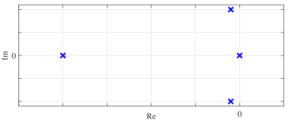
Figure 1: Typical poles configuration of oscillatory system (2), (2).

Then, the associated fourth-order input-output transfer function (2) can be rewritten as

$$G(s)=\frac{N(s)}{D(s)}=\frac{k(s+z_{1})}{s(s+p_{1})(s^{2}+2\zeta\omega_{0}s+\omega_{0}^{2})}.$$ (3)

Here the system parameters are accommodated in the gain factor $k$, natural frequency $\omega_{0}$, damping ratio $\zeta$, and the roots’ coefficients of one real zero $z_{1}$ and one real pole $p_{1}$, while $z_{1}>\omega_{0}$; all coefficients are strictly positive. Worth emphasizing that $0<\zeta\ll 1$, while for $\zeta=1$ the conjugate complex pole pair collapses into the double real pole, and the system (3) becomes critically damped without having to compensate for oscillatory behavior.

Applying any type of the output feedback controller $R(s)$, yet without pole-zero cancelation within $R(s)G(s)$, results in the closed-loop transfer function

$$H(s)=\frac{N(s)}{D(s)+R(s)N(s)}=\frac{N(s)D(s)^{-1}}{1+R(s)N(s)D(s)^{-1}}.$$ (4)

Recall that the loop transfer function $R(s)N(s)D(s)^{-1}$ contains all information about the closed-loop behavior and is (usually) used for analysis and design of the feedback control $R(s)$, which should render a desired $H(s)$-behavior, cf. e.g. [12, 13]. Due to the phase lag of the fourth-order dynamics (3), the output feedback capacities are relatively limited, featured by the stability margins, and more specifically – gain and phase margins. An increase of the loop gaining factor, i.e. either of $k$ in (3) or $R(0)$ of the control, leads unavoidably to destabilization of $H(s)$. This is due to the lack of the gain margin (GM) of the loop transfer function $R(s)N(s)D(s)^{-1}$ once a proportional feedback is included in $R(s)$. Worth emphasizing is that without compensating explicitly for the resonance peak at $\omega_{0}$ and, therefore, improving the GM criteria of the loop transfer characteristics, any type of $R(s)$ with proportional feedback action will lead to an unstable, or at least largely oscillating, behavior of $H(s)$. This becomes best way visible when comparing the loop transfer functions $N(s)D(s)^{-1}$ for two largely differing damping ratios, e.g. $\zeta=[0.01,0.7]$. This results in a frequency response with and without resonance peak as exemplary shown in Figure 2.

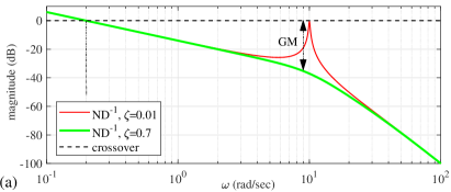
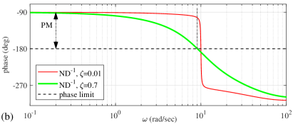
Figure 2: Exemplary Bode diagrams of the loop transfer functions $N(s)D(s)^{-1}$ with different damping ratios $\zeta=[0.01,0.7]$.

While the phase margin (PM) appears sufficient and nearly unsensitive to the damping ratio, for the assigned loop gaining factor, the GM is drastically reduced in case of the resonance peak. The GM of the loop transfer function with $\zeta=0.7$, marked by the double-arrow in Figure 2, will only gradually decrease with an increasing gain factor. Quite opposite, for the loop transfer function with $\zeta=0.01$, an infinitesimally small gain enhancement will already lead to losing completely GM and, therefore, to destabilization of $H(s)$.

Against the background provided above, the objective is to design the time-delay-based output feedback compensator $R(s)$, which will largely attenuate the resonance peak of the system (3) without significantly affecting the residual shape of the loop transfer function. This way, a time-delay-based compensation should allow for using other outer feedback control loops which can guarantee for $x(t)-r(t)\rightarrow 0$, where $r=\mathrm{const}\neq 0$ is a reference set value, and that after possibly oscillation-free transient response of the control system.

3 Time-delay feedback control

The proposed control (1) is parameterized by the gain factor $K_{d}>0$ and the time-delay

$$\tau=-\bigl{[}\arg G(j\omega)|_{\omega=\omega_{0}}\bigr{]}\omega_{0}^{-1}.$$ (5)

The latter corresponds to the phase angle at the resonance frequency, where the output value is in anti-phase (i.e. $-\pi$ rad/s) to the input value. Though an explicit use of the time delay in output feedback was proposed previously for the second-order systems in [6], the control (1), (5) is principally differing to that one provided in [6]. The difference between the current and anti-phase-delayed output values in (1) provides a nearly zero or some low-constant control action for all angular frequencies other than $\omega_{0}$. On the contrary, in vicinity to $\omega_{0}$ the proposed control aims to suppress the resonance peak, cf. Figure 2, through the positive feedback of the control law (1).

Despite the dynamic behavior of systems with time delay are usually analyzed in time domain, cf. [8], [7], [2], we purposefully use the frequency domain consideration of the system transfer characteristics, this way allowing for stability margin analysis and corresponding loop shaping via time delay in feedback. Here it is worth mentioning that the stability of time-delay systems by considering the induced-gain of a time-delay operator in the loop and the associated Bode plots were successfully analyzed in [14].

Taking the ratio between the uncompensated loop transfer function (3) and feedback-compensated (4) results in

$$\frac{G(s)}{H(s)}=1+\frac{R(s)N(s)}{D(s)}.$$ (6)

For achieving the above stated compensation goals, cf. with Figure 2, one needs to ensure that (6) has the magnitude response satisfying $|G(j\omega)||H(j\omega)|^{-1}=\mathrm{const}$ for $\omega<\omega_{0}$ and $|G(j\omega)||H(j\omega)|^{-1}=\mathrm{const}\approx 1$ for $\omega>\omega_{0}$. This is in the sense of loop shaping where the resonance peak associated with $\omega_{0}$ needs to be suppressed. Recall that here, $H(j\omega)$ constitutes a resonance compensated loop transfer function, cf. with exemplary frequency characteristics shown in Figure 2 for the well damped case of $\zeta=0.7$. Note that at lower frequencies $\omega<\omega_{0}$, the loop gaining factor of (6) can be adjusted afterwards, this way settling the required crossover frequency once the resonance peak is compensated. For angular frequencies around $\omega_{0}$, the (6) ratio must be of the same magnitude as the resonance peak of $G(j\omega)$, meaning its maximal possible compensation.

Before deriving the corresponding optimal $K_{d}$-gain, for which the resonance peak is attenuated as possible at $\omega_{0}$, let us first examine the principal ability of

$$R(s)=K_{d}\bigl{(}\exp(-s\tau)-1\bigr{)}$$ (7)

to meet the above requirements at lower and higher frequencies, i.e. for $\omega<\omega_{0}$ and $\omega>\omega_{0}$. Recall that the time-delay-based compensator (7), as infinite-dimensional operator, is upper bounded by a lead transfer element with the gaining factor $2K_{d}$, cf. Figure 3 and e.g. [13, ch. 4].

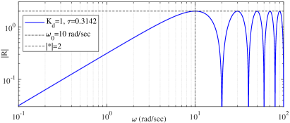
Figure 3: Exemplary magnitude plot of (7) with $K_{d}=1$, $\tau=0.3142$.

Since for $\omega<\omega_{0}$ the $|D(j\omega)|$ has also an incremental slope of one decade per decade and $|N(j\omega)|\rightarrow\mathrm{const}=kz_{1}$, it is apparent that $|R(j\omega)N(j\omega)D^{-1}(j\omega)|=\mathrm{const}$ at lower frequencies, cf. (6). Note that this constant value depends on both, the system parameter $kz_{1}$ and the control parameter $\tau$. At higher frequencies, $|D(j\omega)|$ has an incremental slope of four decades per decade, owing to four integrators in a chain, see (3). At the same time, $|N(j\omega)|$ has an incremental slope of one decade per decade and $|R(j\omega)|\leq\mathrm{const}$ for $\omega>\omega_{0}$, cf. Figure 3. Therefore, $|R(j\omega)N(j\omega)D^{-1}(j\omega)|\rightarrow 0$ as $\omega$ increases within the range larger than $\omega_{0}$. An exemplary $G(s)H(s)^{-1}$ ratio is demonstrated by the magnitude plot in Figure 4, here for the sake of visualization.

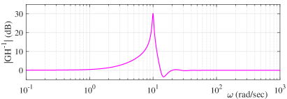
Figure 4: Exemplary plot of $|GH^{-1}|$ ratio according to (6), (7).

In order to determine the optimal $K_{d}$-gain, consider first the resonance peak of $G(j\omega)$ comparing to the transfer characteristics of $G$ without resonance peak, i.e. for $\zeta=0.7$. For the natural frequency, one obtains

$$\frac{|G(j\omega_{0})|}{|G_{\zeta=0.7}(j\omega_{0})|}=\frac{0.7}{\zeta},$$ (8)

which indicates the desired ratio of (6) at $\omega=\omega_{0}$ when applying a suitable $R(s)$. Replacing in (6) the left-hand-side by (8) and $R(s)$ by (7), substituting $j\omega$ instead of $s$, and solving the obtained equation for $\omega=\omega_{0}$ results in

$$K_{d}=\frac{\omega_{0}^{3}(0.7-\zeta)}{k}\,\Bigl{|}\frac{p_{1}+j\omega_{0}}{z_{1}+j\omega_{0}}\Bigr{|}.$$ (9)

4 Stabilization of non-collocated PI-control

For non-collocated output of the system (3) to be controlled, an inherent stability problem lies in the fact of a phase ’deficit’ due to the system relative degree $>2$. The $\angle G$ is always crossing the $-180$ deg phase limit, cf. Figure 2, thus making the GM to a sensitive stability criteria. Needless to say is that additional unmodeled lag properties in the loop with system $G(s)$, such as due to even minor dynamics of sensing and actuating elements and signal transmission delays, will further increase the phase ’deficit’ and, thus, impair stability margins in general.

In order to guarantee the controlled output $x(t)$ can follow the reference value $r(t)$, i.e. to solve not only a set value stabilization problem $r=\mathrm{const}$, an integral control term is usually required. When applying a standard PI (proportional-integral) controller, with the design parameters $K_{p},K_{i}>0$, the loop transfer function is written

$$L(s)=C(s)G(s)=K_{p}\,\frac{s+K_{i}K_{p}^{-1}}{s}\,\frac{N(s)}{D(s)}.$$ (10)

It is remarkable that independent of the assigned $K_{p},K_{i}$ a conjugate-complex pole pair of $L(s)$ does not vanish, cf. Figure 1, and is migrating to the right towards the unstable right-hand-side half plane when increasing the loop gain factor $K_{p}$. Using, for example, the root locus analysis or other conventional tools of the linear control theory, cf. [12], one can find the critical $\max K_{p}$ beyond which the closed loop of (10) becomes unstable. Even if $K_{p}<\max K_{p}$ is guaranteed, the uncertainties in $k$ or its temporal variations, cf. (3), can destabilize the closed-loop system. Furthermore, a lower loop gain cannot improve the transient oscillating behavior since the damping ratio of the conjugate-complex pole pair is not directly affected by the design of $K_{p},K_{i}$.

In order to see the stabilizing properties of the time-delay-based compensator (7), the $G(s)$ and $D(s)$ must be substituted in (10) by $H(s)$ and $D(s)+R(s)N(s)$, respectively. Then, the phase characteristics and, thereupon based, stability margins are visible when comparing $\angle\,\bigl{(}D(j\omega)\bigr{)}^{-1}$ and $\angle\,\bigl{(}D(j\omega)+R(j\omega)N(j\omega)\bigr{)}^{-1}$, see Figure 5.

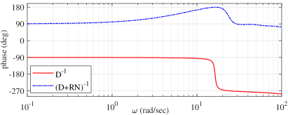
Figure 5: Exemplary phase characteristics of $D^{-1}$ and $(D+RN)^{-1}$.

One can recognize that the lifted and reshaped phase response of the loop transfer function with $H(j\omega)$ does not cross $\pm 180$ deg phase limits over the whole frequency range. This allows for larger variations of the loop gains $K_{p}$ and $k$, in addition to the resonance peak cancelation and, thus, improvement of GM criterion, cf. section 3.

Combining the outer PI control $C(s)$ and the time-delay-based compensation $R(s)$ results in the overall two-degrees-of-freedom feedback controller

$$u(s)=C(s)r(s)+\bigl{(}R(s)-C(s)\bigr{)}x(s).$$ (11)

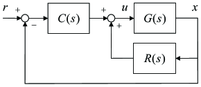
Figure 6: Block diagram of the control loop with feedback controller $C(s)$ and stabilizing compensator $R(s)$

This is purposefully denoted to have two degrees-of-freedom since the compensator $R(s)$ is designed fully independently of $C(s)$. This is equivalent to the outer control of the resonance compensated system $H(s)=x(s)/v(s)$, where the new (virtual) input is $v(s)=u(s)-R(s)y(s)$. The structure of the overall two-degrees-of-freedom control loop with (11) is visualized in the block diagram in Figure 6, for convenience of the reader.

5 Experimental example

In the following, a series of control experiments performed on the laboratory system [11], [15] is provided for evaluating the time-delay-based compensator in accord with sections 3 and 4. The fourth-order system plant is the two-mass oscillator with non-collocated contactless sensing of the load position and actuation by the voice-coil-motor, see Figure 7.

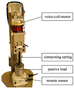
Figure 7: Two-mass oscillator system with non-collocated contactless sensing and voice-coil-motor actuation (laboratory view).

The available actuator displacement is bounded by $0\leq y\leq 0.02$ m. The well-balanced free hanging load (with one vertical degree of freedom) is subject to the oscillations with an extremely low structural damping of the connecting spring, cf. [11] and Figure 9 (a). The input control voltage $U(t)$ of the voice-coil-motor and the relative position $X(t)=x(t)+x_{0}$ of the hanging load are real-time available with the set sampling rate of 10 kHz. The steady-state elongation offset $x_{0}$ is due to the gravity force when $U(t)=0$. The nominal values of the system parameters, partially identified and partially taken over from the technical data sheets, are listed in Table 1, while for more details on the system model we refer to [16]. Since the gravity force of both moving masses $\mathrm{m}_{1}$ and $\mathrm{m}_{2}$ is known and does not change over the operation range, it is pre-compensated, thus resulting in

$$U(t)=u(t)+u_{g}=u(t)+\frac{\mathrm{R}\mathrm{g}}{\Psi}\Bigl{(}\mathrm{m}_{1}+\mathrm{m}_{2}\Bigr{)}.$$ (12)

Here $u(t)$ is the applied feedback control law (11). Further we note that the electromagnetic dynamics of the voice-coil-motor is reasonably neglected, so that the coupling factor between the input (terminal) voltage and the produced electro-magnetic force (EMF) is $\Psi\mathrm{R}^{-1}$.

Table 1: Nominal values of the system parameters.

parameter	unit	value	meaning
$\mathrm{m}_{1}$	kg	0.6	actuator mass
$\mathrm{m}_{2}$	kg	0.75	load mass
$\mathrm{k}$	N/m	200	spring constant
$\sigma$	kg/s	200	actuator damping
$\delta$	kg/s	0.01	spring damping
$\mathrm{R}$	V/A	5.23	coil resistance
$\Psi$	Vs/m	17.16	EMF constant
$\mathrm{g}$	m/s2	9.81	gravity constant

For the vector of the state variables $z\equiv(\dot{y},y,\dot{x},x)^{\top}$, the corresponding state-space model is

$$\dot{z}=\underset{A}{\underbrace{\left(\begin{array}[]{cccc}-333.4&-333.3&0.033&333.3\\ 1&0&0&0\\ 0.027&266.7&-0.027&-266.7\\ 0&0&1&0\end{array}\right)}}z+B\,u,$$ (13)

with the coupling vectors $B=(5.47,0,0,0)^{\top}$ and $F=(0,0,0,1)$ of the input and output, respectively. The natural frequency corresponding to the oscillations of the hanging load is at $\omega_{0}=16.3$ rad/sec. The parameters of the feedback control $u(t)$, given by (11), are $K_{p}=100$, $K_{i}=150$, $K_{d}=100$, $\tau=0.1923$. The corresponding Bode diagrams of the plant $G(j\omega)$ and the plant extended by the time-delayed feedback $H(j\omega)$, both connected in series with the PI-feedback controller $C(j\omega)$, are shown in Figure 8.

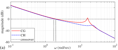
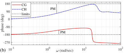
Figure 8: Bode diagrams of the loop transfer functions $CG$ and $CH$.

While the phase margin of the $C(s)G(s)$ loop transfer function is relatively moderate, being $\mathrm{PM}_{CG}=52.3$ deg, the gain margin is not available, i.e. being already negative $\mathrm{GM}_{CG}=-4$ dB. That means an unstable closed-loop behavior of the $C(s)G(s)$ loop system. On the contrary, the $C(s)H(s)$ loop transfer function reveals a sufficiently large phase margin, as $\mathrm{PM}_{CH}=112$ deg, and a theoretically infinite gain margin since $\angle CH$ is not crossing the $\pm 180$ deg phase limits, see Figure 8.

The open-loop response of the experimental system to a short rectangular pulse is shown in Figure 9 (a) and visualizes the low damping properties of the two-mass oscillator.

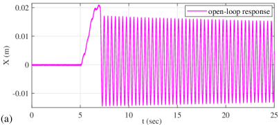
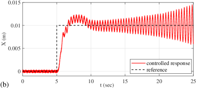
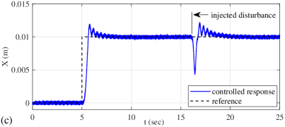
Figure 9: Measured load position: oscillatory open-loop response to a short square-shape pulse excitation in (a), controlled step response with PI feedback only in (b), controlled step response with PI feedback extended by the time-delay compensator (11) in (c).

The unstable step response of the PI-feedback controlled system (i.e. when setting $K_{d}=0$) is shown in Figure 9 (b). On the contrary, the step response of the time-delay-stabilized PI-feedback control system (i.e. when allowing for $K_{d}=100$) is shown in Figure 9 (c). Note that here, an additional external manual disturbance was injected at the time about $t\approx 16.5$ sec, for additional assessment of robustness of the proposed time-delay-based compensator.

6 Summary and Discussion

In this paper, we presented a new time-delay-based control method which allows for a robust compensation of resonance oscillations in non-collocated fourth-order dynamic systems. The compensator has only two parameters, the natural frequency and an adjustable gain factor, the value of which is determined based on the knowledge of resonance peak magnitude of the system transfer characteristics. The analysis of the time-delay-based approach and associated loop shaping are made in frequency domain, also using the stability margins as classical criteria for robustness and performance of an output feedback loop.

It is fair to notice that the proposed control (1), (5) has the induced gain properties which are similar (in magnitude response) to those of the lead transfer element

$$W(s)=\frac{2K_{d}s}{\tau s+1}.$$

The main advantage of the proposed method, however, is that neither time derivatives of the noisy output nor implementation of any transfer functions, like e.g. $W(s)$, are required for applying (1), (5). Also the analytic form (1) of the control law in time domain can allow for adaptation and on-line adjustment of the natural frequency parameter, which speaks for different real applications.

If a non-collocated output feedback system (3) uses a PI control to guarantee the steady-state performance, i.e. $x(t)-r(t)\rightarrow 0$, the feedback control loop yields inherently unstable if not compensating for the resonance peak. The proposed time-delay-based loop shaping suppresses robustly the resonance peak without much affecting the loop transfer characteristics at other frequencies. It is worth noting that the proposed compensator relies on the knowledge of $\omega_{0}$, cf. (5), (9). A robust estimation of $\omega_{0}$, as shown in [15], is however available for tuning the required parameters. It can also be noted that despite uncertainties of $\omega_{0}$, which are due to effective stiffness in the operational point of the oscillator, the compensator performs robustly, as confirmed by the experimental evaluation. A detailed sensitivity analysis of parameter tuning is beyond the scope of this work and is the subject of future research.

The proposed control method was evaluated experimentally on two-mass oscillator system with non-collocated contactless sensing and voice-coil-motor actuation. It was shown, cf. Figure 9, that an extremely low-damped oscillatory behavior is effectively compensated by the proposed time-delay-based method, thus allowing also for a standard PI outer feedback control loop.

References

- [1] W. Michiels, Control of Linear Systems with Delays, Springer, 2013, pp. 1–10.
- [2] E. Fridman, L. Shaikhet, Delay-induced stability of vector second-order systems via simple Lyapunov functionals, Automatica 74 (2016) 288–296.
- [3] R. Sipahi, S.-I. Niculescu, C. T. Abdallah, W. Michiels, K. Gu, Stability and stabilization of systems with time delay, IEEE Control Systems Magazine 31 (1) (2011) 38–65.
- [4] V. Kharitonov, Time-delay systems: Lyapunov functionals and matrices, Springer, 2013.
- [5] E. Fridman, Tutorial on Lyapunov-based methods for time-delay systems, European Journal of Control 20 (6) (2014) 271–283.
- [6] C. Abdallah, P. Dorato, J. Benites-Read, R. Byrne, Delayed positive feedback can stabilize oscillatory systems, in: American Control Conference, 1993, pp. 3106–3107.
- [7] S.-I. Niculescu, W. Michiels, Stabilizing a chain of integrators using multiple delays, IEEE Transactions on Automatic Control 49 (5) (2004) 802–807.
- [8] J.-P. Richard, Time-delay systems: an overview of some recent advances and open problems, Automatica 39 (10) (2003) 1667–1694.
- [9] K. Pyragas, Continuous control of chaos by self-controlling feedback, Physics Letters A 170 (6) (1992) 421–428.
- [10] A. G. Balanov, N. B. Janson, E. Schöll, Control of noise-induced oscillations by delayed feedback, Physica D: Nonlinear Phenomena 199 (1–2) (2004) 1–12.
- [11] M. Ruderman, Robust output feedback control of non-collocated low-damped oscillating load, in: IEEE 29th Mediterranean Conference on Control and Automation (MED), 2021, pp. 639–644.
- [12] S. Skogestad, I. Postlethwaite, Multivariable feedback control: analysis and design, John Wiley & Sons, 2005.
- [13] J. C. Doyle, B. A. Francis, A. R. Tannenbaum, Feedback control theory, Dover, 2009.
- [14] C.-Y. Kao, B. Lincoln, Simple stability criteria for systems with time-varying delays, Automatica 40 (8) (2004) 1429–1434.
- [15] M. Ruderman, One-parameter robust global frequency estimator for slowly varying amplitude and noisy oscillations, Mechanical Systems and Signal Processing 170 (2022) 108756.
- [16] B. Voß, M. Ruderman, C. Weise, J. Reger, Comparison of fractional-order and integer-order H-infinity control of a non-collocated two-mass oscillator, IFAC-PapersOnLine 55 (25) (2022) 145–150.