New charged anisotropic solution on paraboloidal spacetime

Abstract

New exact solutions of Einstein’s field equations for charged stellar models by assuming linear equation of state $P_{r}=A(\rho-\rho_{a})$, where $P_{r}$ is the radial pressure and $\rho_{a}$ is the surface density. By assuming $e^{\lambda}=1+\frac{r^{2}}{R^{2}}$ for metric potential. The physical acceptability conditions of the model are investigated, and the model is compatible with several compact star candidates like 4U 1820-30, PSR J1903+327, EXO 1785-248, Vela X-1, PSR J1614-2230, Cen X-3. A noteworthy feature of the model is that it satisfies all the conditions needed for a physically acceptable model.

1 Introduction

Einstein’s field equations are a system of highly non-linear partial differential second-order equations. They are essential for modeling relativistic compact objects such as dark energy stars, gravastars, quark stars, black holes and neutron stars. The pressure distribution in the star may not be isotropic when the matter distributions have a high density in the nuclear regime, has been presented by Ruderman ruderman1972pulsars and Canuto canuto1974equation . Bowers and Liang bowers1974anisotropic discussed the different causes for anisotropy. Since then, many researchers have studied the anisotropy Maharaj and Maartens maharaj1989anisotropic , Gokhroo and Mehra gokhroo1994anisotropic , Patel and Mehta patel1995exact , Tikekar and Thomas tikekar1998relativistic , Tikekar and Thomas tikekar1999anisotropic , Tikekar and Thomas tikekar2005relativistic , Thomas and Ratanpal thomas2007non , Dev and Gleiser dev2002anisotropic , Dev and Gleiser dev2003anisotropic , Dev and Gleiser gleiser2004anistropic to name a few. A large number of researchers worked on Einstein’s field equations, making different assumptions in the physical content as well as spacetime metric viz., Sharma and Ratanpal sharma2013relativistic , Murad and Fatema murad2013family , Murad and Fatema murad2014some , Murad and Fatema murad2015some , Pandya et al. pandya2015modified , Pandya and Thomas thomas2015compact , Pandya and Thomas thomas2015new , Ratanpal et al. ratanpal2015new .

For constructing relativistic compact star models, an equation of state for the matter content is substituted in Einstein’s field equations. Researchers used generic barotropic equations of state, in which pressure and density have linear, quadratic or polytropic relationships in several modern literary works. Sharma and Maharaj sharma2007class used linear equation of state to establish relativistic compact models consistent with observational data. Physically viable relativistic compact stars models studied by Ngubelanga et al. ngubelanga2015relativistic for a linear equation of state in isotropic coordinates. For getting a solution of anisotropic distributions with a quadratic equation of state (EOS) deliberated by Sharma and Ratanpal sharma2013relativistic , Feroze and Siddiqui feroze2011charged and Takisa and Maharaj takisa2013compact . Thirukkanesh and Ragel thirukkanesh2012exact and Takisa and Maharaj takisa2013some have implemented polytropic EOS to generate results for relativistic stars.

Knutsen knutsen1988some gave the set-up for general conditions like causality condition, regularity condition and strong and weak energy condition. It has been observed that if the tangential pressure (denoted by $p_{\perp}$) is higher than the radial pressure (represented by $p_{r}$), the system becomes more stable. The effect of anisotropy has been derived by Ivanov ivanov2002static . Once Einstein’s field equations are solved using the energy-momentum tensor, using boundary condition with $r=R$, one can obtain the constant of integration and eventually determine the mass and radius of the star. In 2007, Sharma and Maharaj sharma2007class studied the linear equation of state for relativistic stars choosing $e^{\lambda}=\frac{1+ar^{2}}{1+(a-b)r^{2}}$ in the space-time metric as the coefficient of $dr^{2}$, get the different result for different values of $a$ and $b$. Thirukkanesh and Maharaj thirukkanesh2008charged have studied charged anisotropic matter with a linear equation of state by specifying a particular form for one of the gravitational potentials and the electric field intensity. Ivanov ivanov2020linear has studied generating solutions for linear and Ricatti equation in general relativity.

Felice et al. de1999relativistic and Ray et al. ray2003electrically suggested the models generated which have been used in the description of neutron stars and black hole formation. Several models of charged relativistic matter have been studied by researchers, for example, Komathiraj and Maharaj komathiraj2007analytical , Thirukkanesh and Maharaj thirukkanesh2008charged . Bare quark stars were considered by Usov et al. usov2005structure , hybrid proto-neutron stars by Nicotra et al. nicotra2006hybrid and strange quark star matter by Dicus et al. dicus2008critical has been used in charged models. In static spherically symmetric spacetimes, the existence of a conformal killing vector is assumed by Esculpi and Aloma esculpi2010conformal for the anisotropic relativistic charged matter. Mak and Harko mak2002exact have found exact solutions for strange quark matter. Felice et al. de1999relativistic studied a particular solution relating the radial pressure to the energy with a quadratic equation of state. This is a significant advance as the complexity of the model increases significantly due to the radial pressure non-linearity concerning the energy density. But the survey mentioned it mainly suffers from the undesired property of having specificity in the charge density property of the center of the sphere. Malaver malaver2014strange represented a relativistic model with the quadratic equation of state with a charged distribution and a gravitational potential $z(x)$ that depends on an adjustable parameter. Malaver and Daei malaver2020relativistic studied the strange quark star model with the quadratic equation of state to integrate the field equation. Sunzu et al. sunzu2014charged describe matter distribution satisfies a linear equation of state consistent with quark matter. Maharaj et al. maharaj2014some derived some simple models for quark stars by considering the charged anisotropic matter with a linear equation of state.

The objective of this paper is to generate exact solutions to the Einstein field equation, with a linear equation of state that may be derived to analyse charged anisotropic relativistic compact stars. Section 2 expresses the paraboloidal spacetime and the field equations assuming anisotropic matter distributions. In section 3, we derived the model by assuming the linear equation of state $p=p(\rho)$ by taking ansatz $e^{\lambda}=1+\frac{r^{2}}{R^{2}}$. In section 4, finding the parameter R, A and $\alpha$. We have used matching condition for the interior spacetime metric with the Schwarzchild exterior metric across the boundary $r=a$. In section 5, we have found the bounds on A and $\alpha$ by using the feasibility conditions at the centre $r=0$ and on the boundary at $r=a$. We have obtained solutions of EFEs satisfying the linear equation of state on a paraboloidal spacetime compatible with observational data of many compact star candidates like 4U 1820-30, PSR J1903+327, EXO 1785-248, Vela X-1, PSR J1614-2230, Cen X-3. All the physical acceptability conditions have been extensively discussed in section 5. In section 5, we have discussed the physical viability of the model using the graphical method for the compact stars like 4U 1820-30, PSR J1903+327, EXO 1785-248, Vela X-1, PSR J1614-2230, Cen X-3. In section 6, we have concluded by pointing out the main results of our model.

2 The Spacetime Metric

A three-paraboloid immersed in a four-dimensional Euclidean space has the cartesian equation

$$x^{2}+y^{2}+z^{2}=2wR,$$ (1)

where w = constants gives a spheres, while x = constants, y = constants, z = constants respectively, give 3- paraboloids. on taking the parametrization

$$x=rsin\theta cos\phi,$$

$$y=rsin\theta sin\phi,$$

$$z=rcos\theta,$$

$$w=\frac{r^{2}}{2R},$$ (2)

the euclidean metric

$$d\sigma^{2}=dx^{2}+dy^{2}+dz^{2}+dw^{2}.$$ (3)

takes the form

$$ds^{2}=\left(1+\frac{r^{2}}{R^{2}}\right)dr^{2}-r^{2}(d\theta^{2}+sin^{2}\theta d\phi^{2})$$ (4)

We shall take the interior spacetime metric for the anisotropic fluid distribution as

$$ds^{2}=e^{\nu}dt^{2}-\left(1+\frac{r^{2}}{R^{2}}\right)dr^{2}-r^{2}(d\theta^{2}+sin^{2}\theta d\phi^{2})$$ (5)

The constant $\frac{1}{R^{2}}$ can be identified with the curvature parameter. We take the energy-momentum tensor for an anisotropic-charged imperfect fluid sphere to be of the form

$$T_{ij}=diag\left(\rho+{E^{2}},P_{r}-{E^{2}},P_{\perp}+{E^{2}},P_{\perp}+{E^{2}}\right)$$ (6)

where $\rho$ is the matter density, $P_{r}$ is the radial pressure, $p_{\perp}$ is the tangential pressure, and E is the electric field intensity. with spacetime metric (5) and energy-momentum technique (6) the Einstein’s field equations, takes the form

$$8\pi\rho+E^{2}=\frac{1-e^{-\lambda}}{r^{2}}+\frac{e^{-\lambda}\lambda^{\prime}}{r},$$ (7)

$$8\pi p_{r}-E^{2}=\frac{e^{-\lambda}\nu^{\prime}}{r}+\frac{e^{-\lambda}-1}{r^{2}},$$ (8)

$$8\pi p_{\perp}+E^{2}=e^{-\lambda}\left(\frac{\nu^{{}^{\prime\prime}}}{2}+\frac{\nu^{2}}{4}-\frac{\nu^{\prime}\lambda^{\prime}}{4}+\frac{\nu^{\prime}-\lambda^{\prime}}{2r}\right),$$ (9)

$$8\pi\Delta=8\pi P_{r}-8\pi P_{\perp}.$$ (10)

where primes denote differentiation with respect to r. The system of equation (7-10) governs the behaviour of the gravitational field for an anisotropic charged fluid distribution. choosing

$$E^{2}=\frac{\alpha\frac{r^{2}}{R^{2}}}{R^{2}(1+\frac{r^{2}}{R^{2}})^{2}}$$ (11)

By substituting the value of $e^{\lambda}=1+\frac{r^{2}}{R^{2}}$ and $E^{2}$ in the equation (7), we get

$$8\pi\rho=\frac{3+(1-\alpha)\frac{r^{2}}{R^{2}}}{R^{2}(1+\frac{r^{2}}{R^{2}})^{2}}$$ (12)

The expression for density $\rho(r)$ is finite at the centre of the star.

3 Linear Equation of state

We anticipate that the matter distribution should meet a barotropic equation of state for a physically plausible relativistic star $p_{r}=p_{r}(\rho)$. Many researchers have presented their idea on the linear equation of state Sharma and Maharaj sharma2007class , Thirukkanesh and Maharaj thirukkanesh2008charged , Thomas and Pandya thomas2017anisotropic . We consider a linear equation of state between the radial pressure $p_{r}$ and matter density $\rho$ as

$$P_{r}=A\rho-B,$$ (13)

Where A and B are constants. The radius of the star with this pressure distribution is obtained by using the condition

$$P_{r}(r=a)=0,$$

gives,

$$B=A\rho_{a}$$ (14)

We substitute equation (14) in (13) , We get

$$P_{r}=A\rho-A\rho_{a}=A(\rho-\rho_{a})$$ (15)

Applying the equation (15) in equation (8), We get

$$\nu^{\prime}=re^{\lambda}[A(\rho-\rho{a})-(\frac{e^{-\lambda}-1}{r^{2}})-E^{2}],$$

$$\nu^{\prime}=r\left(1+\frac{r^{2}}{R^{2}}\right)\left(\frac{1}{r^{2}+R^{2}}+A\left(\frac{-3R^{2}+a^{2}(\alpha-1)}{(a^{2}+R^{2})^{2}}+\frac{3-\frac{r^{2}}{R^{2}}(1-\alpha)}{R^{2}(r^{2}+R^{2})^{2}}-\frac{r^{2}\alpha}{(r^{2}+R^{2})^{2}}\right)\right),$$ (16)

using equation (16), we get

$$e^{\nu}=c\left(r^{2}+R^{2}\right)^{\left(\frac{\alpha+A(2+\alpha)}{2}\right)}$$

$$\centering\times exp\left[{(A+1)(1-\alpha)\frac{r^{2}}{2R^{2}}-\frac{A}{2}\left(\left(3+(1-\alpha)\frac{a^{2}}{R^{2}}\right)\left(1+\frac{r^{2}}{2R^{2}}\right)\left(1+\frac{a^{2}}{R^{2}}\right)^{-2}\dfrac{r^{2}}{R^{2}}\right)}\right],\@add@centering$$ (17)

Where c is a constant of integration. This is a new exact solution for charged linear equation of state. If we put $\alpha=0$ in the expression of $e^{\nu}$, we get the same expression given by Thomas and Pandya thomas2017anisotropic .

4 Matching Condition

The solutions presented in this work might be related to Einstein’s field equations. The spacetime metric (5) together with (2) should continuously useful with the Reissner-Nordström exterior spacetime

$$ds^{2}=\left(1-\frac{2M}{r}+\frac{Q^{2}}{r^{2}}\right)dt^{2}-\left(1-\frac{2M}{r}+\frac{Q^{2}}{r^{2}}\right)^{-1}dr^{2}-r^{2}(d\theta^{2}+sin^{2}\theta d\phi^{2})$$ (18)

This leads to across the boundary r = a of the star. We get,

$$M =\frac{\frac{a^{3}}{R^{2}}\left(1+(1+\alpha)\frac{a^{2}}{R^{2}}\right)}{2(1+\frac{a^{2}}{R^{2}})^{2}}$$ (19)

$$c =\frac{R^{2}}{(a^{2}+R^{2})^{\frac{(A+1)(2+\alpha)}{2}}}\times F$$ (20)

where,

$$F=exp\left({\frac{1}{4R^{2}}\left({AR^{2}+a^{2}A\alpha-Aa^{2}+2a^{2}\alpha+2A\alpha R^{2}-2a^{2}+2R^{2}\alpha-2R^{2}}\right)}\right)$$

The expression of matter density, radial pressure and tangential pressure then takes the form

$$8\pi\rho=\frac{3+(1-\alpha)\frac{r^{2}}{R^{2}}}{R^{2}(1+\frac{r^{2}}{R^{2}})^{2}},$$ (21)

$$P_{r}=A\rho-A\rho_{a}=A(\rho-\rho_{a}),$$ (22)

$$8\pi P_{\perp}=\frac{-r^{2}\alpha}{(r^{2}+R^{2})^{2}}+\frac{A_{1}+A_{2}+A_{3}-A_{4}+r^{2}(A_{5})^{2}}{4(1+\frac{r^{2}}{R^{2}})}.$$ (23)

Where

$$A_{1}=\frac{-18Ar^{2}R^{2}-12AR^{4}+4R^{2}a^{2}A(\alpha-1)+6a^{2}Ar^{2}(\alpha-1)}{R^{2}(a^{2}+R^{2})^{2}},$$

$$A_{2}=\frac{4\alpha R^{2}+4A(2+\alpha)R^{2}-4R^{2}+2(1+A)r^{2}(\alpha+1)}{R^{2}(r^{2}+R^{2})^{2}},$$

$$A_{3}=\frac{-6r^{2}\alpha-6Ar^{2}(2+\alpha)}{(r^{2}+R^{2})^{2}},$$

$$A_{4}=\frac{4(1+A)(\alpha-1)}{R^{2}},$$

$$A_{5}=\frac{A(r^{2}+R^{2})(-3R^{2}+a^{2}(\alpha-1))}{R^{2}(a^{2}+R^{2})^{2}}-\frac{(1+A)(\alpha-1)}{R^{2}}+\frac{\alpha}{r^{2}+R^{2}}+\frac{A(2+\alpha)}{r^{2}+R^{2}}.$$

It connects the variable A, R,$\alpha$ and c. This shows that there are enough parameters to readily satisfy the persistence of the metric coefficients throughout the boundary of the star $r=R$. The amount of free parameters readily meets the requirements that develop for a specific model under research. While putting the variables into the expression $\rho$, $p_{r}$ and $p_{\perp}$, we can observe a graphical representation of different stars at the center and boundary of the star in the next section.

5 Physical Plausibility Condition

Kuchowicz kuchowicz1972differential , Buchdahl buchdahl1979regular , Knutsen knutsen1988some and Murad and Fatema murad2015some have given the set of conditions to verify the model is physically justifiable: (i) Regularity of metric potential (ii) Radial Pressure and Tangential Pressure at the boundary (iii) Energy conditions (iv) Monotone Decrease of Physical Parameters (v) Pressure Anisotropy (vi) Surface Redshift (vii) Stability Conditions (viii) Mass-Radius Relation (ix) Stability under three forces acting on the system

5.1 Regularity of metric potential

In our metric , at $r=0$ , $e^{\lambda}=1$ and

$$e^{\nu}=cR^{\left(\alpha+A(2+\alpha)\right)}e^{\frac{AR^{2}(-3R^{2}+a^{2}(\alpha-1))-2(A+1)R^{2}(\alpha-1)(a^{2}+R^{2})^{2}}{4(a^{2}+R^{2})^{2}}}$$

which are positive constants.

$$(e^{\lambda})^{\prime}=\frac{2r}{R^{2}},\;\;\;\;i.e\;\;\;(e^{\lambda})^{\prime}_{(r=0)}=0$$ (24)

$$(e^{\nu})^{\prime}_{(r=0)}=0$$ (25)

Clearly, from the above equation, it shows that metric coefficients are regular at $r=0$.

5.2 Radial Pressure and Tangential Pressure at Boundary

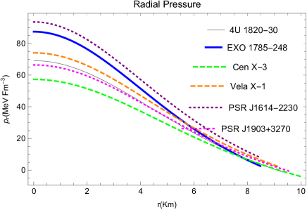
Figure 2: Variation of radial pressures against radial variable $r$.

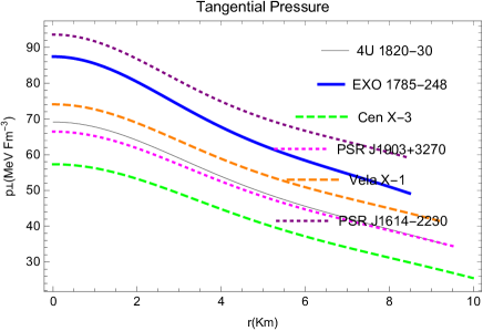
Figure 3: Variation of transverse pressures against radial variable $r$.

The value of radial pressure $p_{r}$ should be equal to zero at the surface of the star $r=a.$ From the equation (22), we can observed that the value of $p_{r}$ at $r=a$ is zero. From equations (22) and (23), it can be shown that the conditions $p_{r}(r=0)\geq 0$ , $p_{\perp}(r=0)\geq 0$ and $p_{\perp}(r=R)\geq 0$ impose a bound on $\alpha$, viz.,$0\leq\alpha\leq 0.251789$. It means that these conditions are satisfied in the range $\alpha$. It can be observed from the graphical method. Fig. 2 and Fig. 3 show that the fact about the condition is satisfied. These conditions are satisfies for the stars 4U 1820-30, PSR J1903+327, EXO 1785-248, Vela X-1, PSR J1614-2230, Cen X-3.

5.3 Pressure Anisotropy

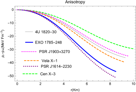
Figure 6: Variation of anisotropies against radial variable $r$.

The difference between tangential and radial pressure should be zero at the centre of a compact star. This condition gives that the pressure components would be equal at a single point. i.e.$\Delta_{(r=0)}=0$ where $\Delta$ is anisotropy of the star. Equation (10) is the expression for the anisotropy. Fig. 6 represents the anisotropy for a different star.

Table 1: Estimated values of physical parameters based on the observational data for $\alpha=0.1$

STAR	$\mathbf{M}$	$\mathbf{a}$	$\mathbf{R}$	$\mathbf{\rho-p_{r}-2p_{\perp}}_{(r=0)}$	$\mathbf{\rho-p_{r}-2p_{\perp}}_{(r=a)}$
	$\mathbf{(M_{\odot})}$	$\mathbf{(Km)}$	(Km)	(MeV fm-3)	(MeV fm-3)
4U 1820-30	1.58	9.1	9.31	834.813	279.409
PSR J1903+327	1.66	9.438	9.54	793.228	258.666
EXO 1785-248	1.3	8.849	8.48	993.993	286.58
Vela X-1	1.77	9.56	8.45	846.824	246.009
PSR J1614-2230	1.97	9.69	9.19	984.427	219.801
Cen X-3	1.49	9.178	9.98	809.696	275.308

In Table 1, We have calculated the values of strong energy condition for various stars at the boundary $(r=a)$ and at center $(r=0)$, which is one of the required conditions to justify the model’s feasibility of compact stars.

5.4 Monotone Decrease of Physical Parameters

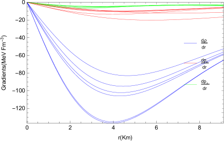
Figure 11: Variation of a Gradients $\frac{d\rho}{dr}$,$\frac{dp_{r}}{dr}$ and $\frac{dp_{\perp}}{dr}$ for different compact stars.

The conditions for monotone decrease of physical parameters are as   $\frac{d\rho}{dr}\leq 0$ ,   $\frac{dp_{r}}{dr}\leq 0$    and    $\frac{dp_{\perp}}{dr}\leq 0$    for $0\leq r\leq a.$ The gradients of density and radial pressure are given by $\dfrac{dp_{r}}{dr}=A(8\pi\dfrac{d\rho}{dr})=A(\frac{2r^{3}(\alpha-1)-2rR^{2}(5+\alpha)}{(r^{2}+R^{2})^{3}})$    for $0\leq r\leq a.$ Fig. 11 shows a gradient of density, radial pressure and tangential pressure are decreasing radially outward for the compact stars 4U 1820-30, PSR J1903+327, EXO 1785-248, Vela X-1, PSR J1614-2230, Cen X-3.

5.5 Energy conditions

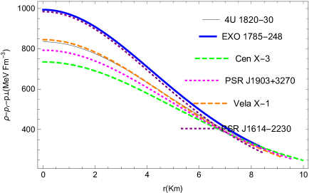
Figure 7: Variation of strong energy condition against radial variable $r$.

(i) $\rho-p_{r}-2p_{\perp}\geq 0$ (Strong energy conditions).
The verification of strong energy condition is verified in Table 1 Strong energy conditions $\rho-p_{r}-2p_{\perp}\geq 0$ at the centre $r=0$ and surface of the star $r=R.$ when we simplify this condition on $\alpha$, we get the restriction on $\alpha$ viz., $0\leq\alpha\leq 0.3215$. The condition is fulfilled within the range of $\alpha$. Fig. 7 is the evidence for the fulfilment of the condition for different stars 4U 1820-30, PSR J1903+327, EXO 1785-248, Vela X-1, PSR J1614-2230, Cen X-3.
(ii) $\rho\geq p_{r}$ and $\rho\geq p_{\perp}$ (Weak Energy conditions).
The Weak energy indicates that $\rho-p_{r}\geq 0$ and $\rho-p_{\perp}\geq 0$. Since the strong energy condition yields a positive value indicating that $\rho$ is greater than both $p_{r}$ and $p_{\perp}.$ This implies that the difference between $\rho$ and $p_{r}$ as well as $\rho$ and $p_{\perp}$ is greater than equal to zero.

5.6 Stability Conditions

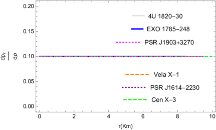
Figure 4: Variation of $\frac{dp_{r}}{d\rho}$ against radial variable $r$.

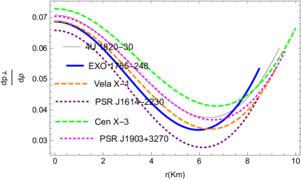
Figure 5: Variation of $\frac{dp_{\perp}}{d\rho}$ against radial variable $r$.

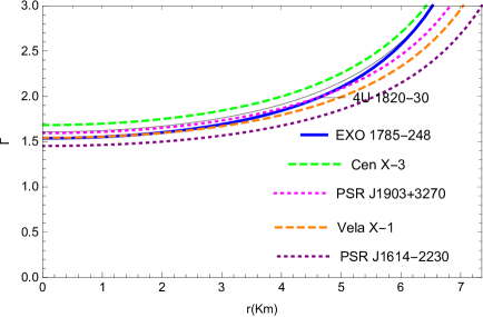
Figure 8: Variation of adiabatic Index against radial variable $r$.

(i) Causality condition: $0\leq\frac{dp_{r}}{d\rho}\leq 1,\;\;0\leq\frac{dp_{\perp}}{d\rho}\leq 1$    for $0\leq r\leq a.$
The values for the radial speed of sound waves $\frac{dp_{r}}{d\rho}$ denoted as $\nu^{2}_{r}$ and transverse speed of sound waves $\frac{dp_{\perp}}{d\rho}$ denoted as $\nu^{2}_{t}$ between $r=0$ and $r=a$ for different stars have been calculated in Table 3. These velocities are in the range of 0 and 1. The bounds on $\alpha$ for $0\leq\frac{dp_{r}}{d\rho}\leq 1,\;\;0\leq\frac{dp_{\perp}}{d\rho}\leq 1$ are $0\leq\alpha\leq 2.28165\;\;and\;\;0\leq\alpha\leq 1.11724$. Fig. 4 and Fig. 5 show that these conditions are satisfied throughout the distribution.
(ii) Relativistic adiabatic index: $\Gamma=(\frac{\rho+p_{r}}{p_{r}})\frac{dp_{r}}{d\rho}$
The adiabatic index stated must be greater than 1.333… in the prescribed range $0\leq r\leq a.$ $\Gamma\geq\frac{4}{3}$ at $r=0$ imposes a restriction on $\alpha$ given by $0\leq\alpha\leq 1.8686$. Table 3 shows these respective values for the different compact stars. Fig. 8 shows that these conditions are satisfied throughout the distribution.

5.7 Redshift

The redshift $z=\sqrt{1/e^{\nu}}-1$ must be a decreasing function of r and finite for $0\leq z\leq 5$. In Table 2, we have described all the values for different compact stars (related to the stability of a relativistic anisotropic stellar configuration). The value of the redshift remains less than 5. For a relativistic star, it is expected that the redshift must decrease towards the boundary and be finite throughout the distribution. Fig. 9 shows that gravitational redshift decreases throughout the star under consideration for 4U 1820-30, PSR J1903+327, EXO 1785-248, Vela X-1, PSR J1614-2230, Cen X-3.

5.8 Mass-Radius Relation:

According to Buchdahl buchdahl1979regular , the mass radius relation must satisfy the inequality, $\frac{M}{a}\leq\frac{4}{9}$ The values are calculated in Table 2 to verify this inequality. We can verify this Mass-Radius Relation with graphical Method $\frac{M}{a}=0.256<\frac{4}{9}.$ Fig. 10 shows the Mass-Radius Relation for the star 4U 1820-30, PSR J1903+327, EXO 1785-248, Vela X-1, PSR J1614-2230 and Cen X-3.

5.9 Stability under three forces acting on the system

We want to examine the stability of our present model under three different forces viz., gravitational force, hydrostatics force and anisotropic force, which the following equation can describe

$$-\frac{M_{G}(r)(\rho+p_{r})}{2}e^{(\nu-\lambda)/2}-\dfrac{dp_{r}}{dr}-\frac{2}{r}(p_{\perp}-p_{r})=0$$ (26)

proposed by Tolman-Oppenheimer-Volkov and named as TOV equation. The quantity $M_{G}(r)$ represents the gravitational mass within the radius r, which can be derived from the Tolman-Whittaker formula and Einstein’s field equations and is defined by

$$M_{G}(r)=\frac{\nu^{\prime}}{2}re^{(\nu-\lambda)/2}$$ (27)

Adding the value of (27) into equation (26), we get,

$$-\frac{\nu^{\prime}}{2}re^{(\nu-\lambda)/2}(\rho+p_{r})e^{(\nu-\lambda)/2}-\dfrac{dp_{r}}{dr}-\frac{2}{r}(p_{\perp}-p_{r})=0$$ (28)

The above expression may also be written as

$$F_{g}+F_{h}+F_{a}=0$$ (29)

$$F_{g}=-\frac{\nu^{\prime}}{2}r(\rho+p_{r})$$ (30)

$$F_{h}=-\dfrac{dp_{r}}{dr}$$ (31)

$$F_{a}=-\frac{2}{r}(p_{\perp}-p_{r})$$ (32)

5 the three different forces act on the system. The figure shows that gravitational 5force is negative and dominating in nature which is counterbalanced by the combined effect of hydrostatics and anisotropic forces to keep the system in equilibrium. Fig. 12 shows these three forces in graphical method for the star 4U 1820-30, PSR J1903+327, EXO 1785-248, Vela X-1, PSR J1614-2230, Cen X-3.

Table 2: Estimated values of physical parameters based on the observational data for $\alpha=0.1$

STAR	$\mathbf{M}$	$\mathbf{a}$	$\mathbf{Z_{r=0}}$	$\mathbf{Z_{(r=a)}}$	$\mathbf{\Gamma_{(r=0)}}$	$\mathbf{u(=\frac{M}{a})}$
	$\mathbf{(M_{\odot})}$	$\mathbf{(Km)}$	(Redshift)	(Redshift)	(Adiabatic	(Buchdahl
					Index)	Ratio)
4U 1820-30	1.58	9.1	0.800561	0.398355	1.60715	0.173
PSR J1903+327	1.66	9.438	0.822543	0.406674	1.59342	0.175
EXO 1785-248	1.3	8.849	0.902282	0.425903	1.53685	0.146
Vela X-1	1.77	9.56	0.921587	0.442963	1.53998	0.185
PSR J1614-2230	1.97	9.69	1.1548	0.521521	1.45172	0.203
Cen X-3	1.49	9.178	0.787317	0.393294	1.61581	0.162

Table 3: Estimated values of physical parameters based on the observational data for $\alpha=0.1$

STAR	$\mathbf{M}$	$\mathbf{a}$	$\mathbf{\left(\frac{dp_{r}}{d\rho}\right)}_{r=0}$	$\mathbf{\left(\frac{dp_{\perp}}{d\rho}\right)_{r=0}}$	$\mathbf{(\nu^{2}_{t}-\nu^{2}_{r})_{r=0}}$	$\mathbf{\left(\frac{dp_{r}}{d\rho}\right)_{r=a}}$	$\mathbf{\left(\frac{dp_{\perp}}{d\rho}\right)_{r=a}}$	$\mathbf{(\nu^{2}_{t}-\nu^{2}_{r})_{r=a}}$
	$\mathbf{(M_{\odot})}$	$\mathbf{(Km)}$
4U 1820-30	1.58	9.1	0.1	0.0707929	-0.0292071	0.1	0.0567916	-0.043
PSR J1903+327	1.66	9.438	0.1	0.0703981	-0.0296019	0.1	0.0572536	-0.042
EXO 1785-248	1.3	8.48	0.1	0.0686885	-0.0313115	0.1	0.0599306	-0.043
Vela X-1	1.77	9.56	0.1	0.0658326	-0.0312131	0.1	0.442963	-0.040
PSR J1614-2230	1.97	9.69	0.1	0.0687869	-0.0341674	0.1	0.0675101	-0.032
Cen X-3	1.49	9.178	0.1	0.071038	-0.028962	0.1	0.0565314	-0.048

6 Discussion

We have studied the compatibility of the model developed using Linear Equation of state in the background of paraboloidal spacetime for compact stars like 4U 1820-30, PSR J1903+327, EXO 1785-248, Vela X-1, PSR J1614-2230, Cen X-3. Our model satisfies the elementary physical requirements for representing a superdense compact star through the graphical method. It is found that the model can accommodate the mass and radius of the compact star candidates given by Gangopadhyay et al. gangopadhyay2013strange . It is found that stars whose compactness is more accommodate more density, pressure and anisotropy. The redshift increase with compactness while the value of the adiabatic Index decreases with compactness showing that the stability decreases with an increase in compactness. Pertinent feature of the model is that the exact solution obtained is simple, which is only found in some solutions. We have displayed the physical analysis only for a few compact star models here, but it can be applied to a larger class of known pulsars. The model possesses a definite background spacetime geometry, namely paraboloidal geometry, and the expression involved in the solution is exponential. It has been concluded that a large number of pulsars with known masses and radii can be accommodated in the present model, satisfying the linear equation of state.

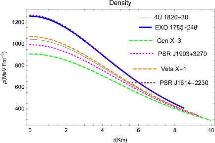
Figure 1: Variation of density against radial variable $r$.

Figure 9: Variation of surface redshift against radial variable $r$.

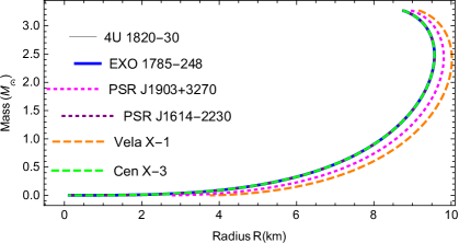
Figure 10: Variation of a mass M with respect to a radius R for various stars.

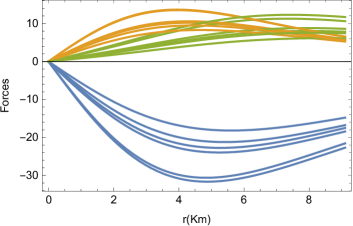
Figure 12: Variation of three forces like Gravitational Force(Blue), Hydrostatic Force(Orange) and Anisotropic Force(Green) for different compact star.

References

- \bibcommenthead
- (1) Ruderman, M.: Pulsars: structure and dynamics. Annual Review of Astronomy and Astrophysics 10(1), 427–476 (1972)
- (2) Canuto, V.: Equation of state at ultrahigh densities. Annual Review of Astronomy and Astrophysics 12(1), 167–214 (1974)
- (3) Bowers, R.L., Liang, E.: Anisotropic spheres in general relativity. The Astrophysical Journal 188, 657 (1974)
- (4) Maharaj, S., Maartens, R.: Anisotropic spheres with uniform energy density in general relativity. General relativity and gravitation 21(9), 899–905 (1989)
- (5) Gokhroo, M., Mehra, A.: Anisotropic spheres with variable energy density in general relativity. General relativity and gravitation 26(1), 75–84 (1994)
- (6) Patel, L., Mehta, N.: An exact model of an anisotropic relativistic sphere. Australian Journal of Physics 48(4), 635–644 (1995)
- (7) Tikekar, R., Thomas, V.: Relativistic fluid sphere on pseudo-spheroidal space-time. Pramana 50(2), 95–103 (1998)
- (8) Tikekar, R., Thomas, V.: Anisotropic fluid distributions on pseudo-spheroidal spacetimes. Pramana 52(3), 237–244 (1999)
- (9) Tikekar, R., Thomas, V.: A relativistic core-envelope model on pseudospheroidal space-time. Pramana 64(1), 5–15 (2005)
- (10) Thomas, V., Ratanpal, B.: Non-adiabatic gravitational collapse with anisotropic core. International Journal of Modern Physics D 16(09), 1479–1495 (2007)
- (11) Dev, K., Gleiser, M.: Anisotropic stars: exact solutions. General relativity and gravitation 34(11), 1793–1818 (2002)
- (12) Dev, K., Gleiser, M.: Anisotropic stars ii: stability. General relativity and gravitation 35(8), 1435–1457 (2003)
- (13) Gleiser, M., Dev, K.: Anistropic stars: Exact solutions and stability. International Journal of Modern Physics D 13(07), 1389–1397 (2004)
- (14) Sharma, R., Ratanpal, B.: Relativistic stellar model admitting a quadratic equation of state. International Journal of Modern Physics D 22(13), 1350074 (2013)
- (15) Murad, M.H., Fatema, S.: A family of well behaved charge analogues of durgapal’s perfect fluid exact solution in general relativity. Astrophysics and space science 343(2), 587–597 (2013)
- (16) Murad, M.H., Fatema, S.: Some static relativistic compact charged fluid spheres in general relativity. Astrophysics and Space Science 350(1), 293–305 (2014)
- (17) Murad, M.H., Fatema, S.: Some new wyman–leibovitz–adler type static relativistic charged anisotropic fluid spheres compatible to self-bound stellar modeling. The European Physical Journal C 75(11), 1–21 (2015)
- (18) Pandya, D., Thomas, V., Sharma, R.: Modified finch and skea stellar model compatible with observational data. Astrophysics and Space Science 356(2), 285–292 (2015)
- (19) Thomas, V., Pandya, D.: Compact stars on pseudo-spheroidal spacetime compatible with observational data. Astrophysics and Space Science 360(2), 1–8 (2015)
- (20) Thomas, V., Pandya, D.: A new class of solutions of compact stars with charged distributions on pseudo-spheroidal spacetime. Astrophysics and Space Science 360(2), 1–13 (2015)
- (21) Ratanpal, B., Thomas, V., Pandya, D.: A new class of solutions of anisotropic charged distributions on pseudo-spheroidal spacetime. Astrophysics and Space Science 360(2), 1–9 (2015)
- (22) Sharma, R., Maharaj, S.: A class of relativistic stars with a linear equation of state. Monthly Notices of the Royal Astronomical Society 375(4), 1265–1268 (2007)
- (23) Ngubelanga, S.A., Maharaj, S.D.: Relativistic stars with polytropic equation of state. The European Physical Journal Plus 130(10), 1–5 (2015)
- (24) Feroze, T., Siddiqui, A.A.: Charged anisotropic matter with quadratic equation of state. General Relativity and Gravitation 43(4), 1025–1035 (2011)
- (25) Takisa, P.M., Maharaj, S.: Compact models with regular charge distributions. Astrophysics and Space Science 343(2), 569–577 (2013)
- (26) Thirukkanesh, S., Ragel, F.: Exact anisotropic sphere with polytropic equation of state. Pramana 78(5), 687–696 (2012)
- (27) Takisa, P.M., Maharaj, S.: Some charged polytropic models. General Relativity and Gravitation 45(10), 1951–1969 (2013)
- (28) Knutsen, H.: Some physical properties and stability of an exact model of a relativistic star. Astrophysics and space science 140(2), 385–401 (1988)
- (29) Ivanov, B.: Static charged perfect fluid spheres in general relativity. Physical Review D 65(10), 104001 (2002)
- (30) Thirukkanesh, S., Maharaj, S.: Charged anisotropic matter with a linear equation of state. Classical and Quantum Gravity 25(23), 235001 (2008)
- (31) Ivanov, B.: Linear and riccati equations in generating functions for stellar models in general relativity. The European Physical Journal Plus 135(4), 1–14 (2020)
- (32) de Felice, F., Siming, L., Yunqiang, Y.: Relativistic charged spheres: Ii. regularity and stability. Classical and Quantum Gravity 16(8), 2669 (1999)
- (33) Ray, S., Espindola, A.L., Malheiro, M., Lemos, J.P., Zanchin, V.T.: Electrically charged compact stars and formation of charged black holes. Physical Review D 68(8), 084004 (2003)
- (34) Komathiraj, K., Maharaj, S.: Analytical models for quark stars. International Journal of Modern Physics D 16(11), 1803–1811 (2007)
- (35) Usov, V., Harko, T., Cheng, K.: Structure of the electrospheres of bare strange stars. The Astrophysical Journal 620(2), 915 (2005)
- (36) Nicotra, O., Baldo, M., Burgio, G., Schulze, H.-J.: Hybrid protoneutron stars with the mit bag model. Physical Review D 74(12), 123001 (2006)
- (37) Dicus, D.A., Repko, W.W., Teplitz, V.: Critical charges on strange quark nuggets and other extended objects. Physical Review D 78(9), 094006 (2008)
- (38) Esculpi, M., Aloma, E.: Conformal anisotropic relativistic charged fluid spheres with a linear equation of state. The European Physical Journal C 67(3), 521–532 (2010)
- (39) Mak, M., Harko, T.: An exact anisotropic quark star model. Chinese journal of astronomy and astrophysics 2(3), 248 (2002)
- (40) Malaver, M.: Strange quark star model with quadratic equation of state. arXiv preprint arXiv:1407.0760 (2014)
- (41) Malaver, M., Daei Kasmaei, H.: Relativistic stellar models with quadratic equation of state. International Journal of Mathematical Modelling & Computations 10(2 (SPRING)), 111–124 (2020)
- (42) Sunzu, J.M., Maharaj, S.D., Ray, S.: Charged anisotropic models for quark stars. Astrophysics and Space Science 352(2), 719–727 (2014)
- (43) Maharaj, S., Sunzu, J., Ray, S.: Some simple models for quark stars. The European Physical Journal Plus 129(1), 1–10 (2014)
- (44) Thomas, V., Pandya, D.: Anisotropic compacts stars on paraboloidal spacetime with linear equation of state. The European Physical Journal A 53(6), 1–9 (2017)
- (45) Kuchowicz, B.: Differential conditions for physically meaningful fluid spheres in general relativity. Physics Letters A 38(5), 369–370 (1972)
- (46) Buchdahl, H.: Regular general relativistic charged fluid spheres. Acta Physica Polonica. Series B 10(8), 673–685 (1979)
- (47) Gangopadhyay, T., Ray, S., Li, X.-D., Dey, J., Dey, M.: Strange star equation of state fits the refined mass measurement of 12 pulsars and predicts their radii. Monthly Notices of the Royal Astronomical Society 431(4), 3216–3221 (2013)