Radial-velocity discovery of a second planet in the TOI-1338/BEBOP-1 circumbinary system
(Old title: The First Circumbinary Planet Discovered with Radial Velocities)

We report the detection of a gas-giant planet in orbit around both stars of an eclipsing binary star system that also contains the smaller, inner transiting planet TOI-1338b. The new planet, called TOI-1338/BEBOP-1c, was discovered using radial-velocity data collected with the HARPS and ESPRESSO spectrographs. Our analysis reveals it is a $65.2~{}\rm{M_{\oplus}}$ circumbinary planet with a period of $215.5$ days. This is the first detection of a circumbinary planet using radial-velocity observations alone, and makes TOI-1338/BEBOP-1 only the second confirmed multiplanet circumbinary system to date. We do not detect the smaller inner transiting planet with radial-velocity data, and can place an upper limit on the inner planet’s mass at $21.8~{}\mathrm{M}_{\oplus}$ with $99\%$ confidence. The inner planet is the first circumbinary planet amenable for atmospheric characterisation, using the James Webb Space Telescope.

Circumbinary planets are planets that orbit both stars of a central binary. They were once confined to science fiction, but the discovery of Kepler-16b  (?) paved the way for the discovery of 14 transiting planets in 12 binary systems, by the Kepler  (?) and TESS  (?) missions. Of the 12 transiting circumbinary planet systems discovered to date only one hosts multiple circumbinary planets, Kepler-47. Kepler-47 b, d and c have orbital periods of $49.5$, $187.4$, and $303.2~{}\rm{days}$ respectively  (?), with c’s orbit placing it within the system’s habitable zone. Planet forming disks around binaries are harsh environments for planet formation to take place, and circumbinary planet discoveries provide insights into the formation and migration mechanisms at play in these unique environments  (?, ?, ?, ?, ?).

Of the 14 confirmed transiting circumbinary planets discovered to date, there are only significant mass detections (different from zero at $>2\sigma$) for six of them. These are: Kepler-34 b and 35 b  (?), TIC 17290098 b  (?), Kepler-16 b  (?, ?), Kepler-47 c and d  (?). Where the masses were determined from binary eclipse timing variations (ETV’s) alone. For the remaining eight circumbinary planets only upper limits can be placed on their masses, because the ETV’s are on the order of only seconds or minutes, and hence difficult to measure. Their masses could therefore be much lower than expected and reveal several inflated objects, ideal targets for atmospheric transmission follow-up observations  (?). To correctly characterise these planets, accurate masses are required.

To increase the number of known circumbinary planets, and to provide accurate masses for systems discovered with the transit method, we initiated a radial-velocity observing survey dedicated to circumbinary planet detection called Binaries Escorted By Orbiting Planets (BEBOP)  (?). Systems followed by BEBOP are on average 4 visual magnitudes brighter than circumbinary systems identified with Kepler  (?). Radial velocities are less restricted to the edge-on and shorter orbital periods found by the transit method  (?). Despite initial challenges in bringing radial-velocity precision for binaries down to values where planets can be detected  (?), recent results have produced an independent detection of Kepler-16b with a precision of $1.5~{}\rm m.s^{-1}$, resulting in a planetary mass in agreement with ETV measurements  (?).

The first circumbinary planet discovered by NASA’s Transiting Exoplanet Survey Satellite (TESS)  (?) was TOI-1338 b  (?). TOI-1338 is a low mass eclipsing binary system, which consists of a $1.13~{}\rm M_{\odot}$ F8-type primary star with a visual magnitude of $V=11.7$  (?, ?), and a $0.31~{}\rm M_{\odot}$ M-dwarf companion. This system was already being monitored with radial velocities with HARPS  (?) as part of the BEBOP project, where the target was known as EBLM J0608-59  (?, ?). Radial-velocity data available at the time were unable to detect any trace of TOI-1338b, the Saturn-sized planet announced by Kostov et al. (2020)  (?). To constrain the mass of this planet, we used the ESPRESSO spectrograph at the Very Large Telescope  (?). Meanwhile we continued to observe with HARPS intermittently in order to combine both datasets more easily, and in order to mitigate observatory closures caused by the COVID pandemic. In total, we collected $123$ ESPRESSO, and $61$ HARPS spectra covering a timespan of $1472$ days.

We analyse our radial-velocity data with the diffusive nested sampler implemented in kima  (?), slightly adapted for the purpose of a circumbinary system. We include non Keplerian effects such as gravitational redshift, light time travel  (?, ?, ?) and tidal distortion  (?). In addition, we directly fit for the most important of the Newtonian perturbations, the apsidal precession, which we parameterise by a free parameter, $\dot{\omega}_{\rm bin}$. Further details can be found in the supplementary material, but we note here that a particularly useful feature of kima is that the number of planetary signals in the data can be included as a free parameter in the analysis. The number of planets detected is determined from the ratio of evidence between models with different number of planets. The radial-velocity data favours a one-planet model over a zero-planet model with a ratio of probability (Bayes factor) $>29,000$ (where $>150$ is the typical threshold for detection). The same analysis provides a Bayes factor of only $1.4$ in favour of a two-planet model over a one-planet model, far below the detection threshold. Therefore, only one planetary signal is formally detected in our data.

Figure 1 depicts a histogram of the posterior samples obtained from our analysis. There are two peaks, one at the binary orbital period of $14.6$ days, and a single additional excess at $215.5$ days. Since this periodicity does not correspond to the $95$ day period of the transiting planet  (?), and an outer orbit significantly improves the fit, we conclude the detected planetary signal is likely that of an additional, outer circumbinary planet within the system. We therefore give the system the name BEBOP-1, becoming the first entry in the BEBOP catalogue for circumbinary planets detected with radial velocities, with the new signal being TOI-1338/BEBOP-1c. Figure 2 shows a phase-folded plot of the radial-velocity variation caused by TOI-1338/BEBOP-1c, with a semi-amplitude $K_{\rm{c}}=5.6\pm 1.0~{}\rm{m.s^{-1}}$, corresponding to a minimum mass $m_{\rm c}\sin i_{\rm c}=0.217\pm 0.035~{}\rm M_{Jup}$. The binary’s apsidal precession is found marginally different from zero ($\dot{\omega}_{\rm bin}=66.0^{+65.0}_{-54.7}~{}\rm{arcsec\,year^{-1}}$). Parameters of the binary and planetary orbits, obtained from our model fit to the radial velocities are available in Table 1. We calculate the True Inclusion Probability (TIP)  (?, ?) for our posterior samples which also provides a clear $>99.9\%$ probability of the presence of a planetary signal at a period of $215.5$ days. Further details can be found in the supplementary material.

Stellar magnetic activity can produce periodic modulations in radial velocity over a wide range of timescales sometimes mimicking a planetary companion  (?). To verify if this is the case for the TOI-1338/BEBOP-1c signal, we search for periodic signals in five spectroscopic activity indices (see supplementary material for details).

Stellar activity has been shown to affect most, if not all of these five indices at once  (?). In our case, only two show any signal. Furthermore, at shorter periods neither Ca II H+K nor H$\alpha$ indices produce any significant peak. Combining the stellar radius and projected rotational velocity of TOI-1338/BEBOP-1, a rotation period of $19\pm 3$ days has been reported  (?). We do not find any statistically significant signal at the estimated rotation period.

Our analysis of activity indices rules out any association between the 215 day radial-velocity variation and stellar activity, supporting the hypothesis for TOI-1338/BEBOP-1c’s planetary nature. Further details and figures are provided in the supplementary material.

A visual inspection of TESS lightcurves shows no transit of TOI-1338/BEBOP-1c, however, thanks to orbital circulation, transits are expected to occur in due time. Circumbinary orbits exhibit nodal precession. This changes the orientation of a circumbinary planet’s orbital plane with respect to both the binary and the observer. This makes a planet change from a transiting to a non-transiting configuration  (?, ?) as has been seen in a few systems  (?, ?). Using an analytic criterion  (?, ?), we find that TOI-1338/BEBOP-1c is guaranteed to eventually transit mainly because the binary is so well-aligned with our line of sight ($I_{\rm bin}=89.658^{\circ}$) combined with the rather large size of the primary star ($R_{\rm A}=1.299R_{\odot}$). Whilst TOI-1338/BEBOP-1c will eventually transit, we are unable to predict when and how frequently. Its precession period is of order 119 years, during which time there will be two periods of transitability of a duration depending on TOI-1338/BEBOP-1c’s orbital inclination.

To verify the orbital parameters of our fit we carry out a global stability analysis of the system. This stability analysis shows the system is stable when the two circumbinary planets are in nearly circular and coplanar orbits (see supplementary material). More precisely, the eccentricities of both planets cannot exceed 0.1, in agreement with the best fit solution (Table 1). The inclination of planet c, $i_{\rm c}$, is unconstrained by the radial velocities, however, thanks to orbital stability arguments, it cannot be higher than $40^{\circ}$ with respect to the orbital plane of the binary, corresponding to a maximum mass of $m_{\rm max,c}=0.28~{}\rm M_{Jup}$.

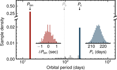
Figure 1: Histogram periodogram of posterior samples obtained from a kima run on the TOI-1338/BEBOP-1 system. The $14.6$ day binary period along with the $215.5$ day period of TOI-1338/BEBOP-1c can be clearly seen, and are highlighted in red and blue respectively. The inlaid plots show a zoom on these two peaks. No significant peak from the transiting planet TOI-1338/BEBOP-1b can be seen in these posterior samples.

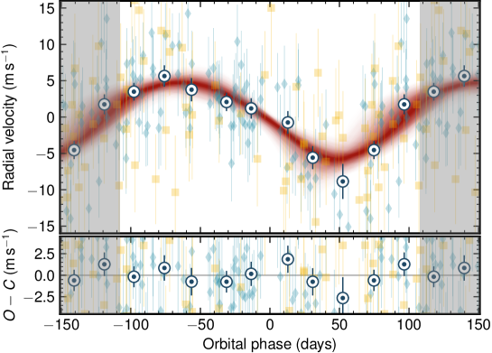
Figure 2: Phased Keplerian Radial-Velocity (RV) models of TOI-1338/BEBOP-1c with ESPRESSO (blue diamonds) and HARPS (orange squares) data along with associated residuals after removing the binary signal. RV data is binned by $0.1$ phase units (${\sim}21.6$ days) and illustrated by the circular points. Red Keplerian models are based on $500$ randomly drawn posterior samples from a kima run, shaded from the $50^{\rm{th}}$ to $99^{\rm{th}}$ percentiles. The shaded regions display the repeating signal.

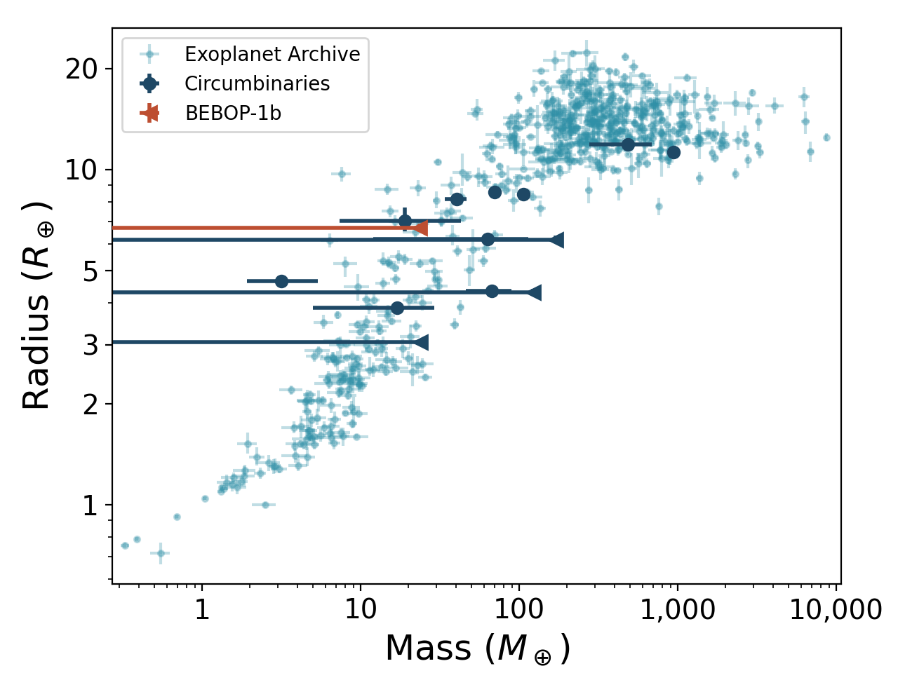
Figure 3: Radius vs Mass plot of all transiting circumbinary planets (dark blue) and planets orbiting single stars (light blue). TOI-1338/BEBOP-1b is highlighted in orange, with one of the lowest densities known. The newly-discovered TOI-1338/BEBOP-1c is not on the graph since it does not transit. For the single star planets we restrict the sample to planets with mass and radius percentage errors less than $20\%$.

The influence of the central binary means that circumbinary planets have unique formation pathways, and it is noteworthy that the system discussed in this paper is only the second system known to host multiple planets. Hydrodynamical simulations have shown that the preference for observed circumbinary planets to be located close to the stability boundary can be explained by formation at large distances in circumbinary discs, followed by inwards migration and stalling at the edge of the inner cavities formed by the central binaries  (?, ?, ?). We have utilised a purpose-built simulation code to study the formation of circumbinary planets as a means of understanding plausible formation scenarios for the TOI-1338/BEBOP-1 system. Details of this code are available in the supplementary material. The model includes the N-body integrator mercury6, adapted to include a central binary system  (?, ?), and it incorporates prescriptions for a viscous circumbinary disc that includes the effects of an eccentric, precessing central cavity and photoevaporative winds  (?), pebble accretion onto planetary seeds  (?), planet migration  (?), and gas accretion onto growing planets  (?, ?). Our suite of simulations produced numerous systems that were qualitatively similar to TOI-1338/BEBOP-1 (see additional material), with TOI-1338/BEBOP-1b and c analogues landing on stable orbits at their observed locations.

With no detection of the $95$ day planet in our data the best we can do is to calculate a detection limit for this period region. We find that TOI-1338/BEBOP-1b has a mass $<~{}21.8\rm~{}M_{\oplus}$ with $99\%$ confidence. This is compatible with the $33\pm 20~{}\rm M_{\oplus}$ from ETV’s  (?). Combined with a planetary radius of $\approx 6.9~{}\rm R_{\oplus}$  (?), TOI-1338/BEBOP-1b has a maximum mean planetary density $<0.36~{}\rm{g.cm^{-3}}$. This allows us to calculate the Transmission Spectroscopy Metric (TSM)  (?) for planet b using the upper limit on the mass ($<~{}21.8\rm~{}M_{\oplus}$); this yields a minimum TSM value of $>39$ (see supplementary material). Of the now 15 known circumbinary exoplanets, TOI-1338/BEBOP-1b is the only one for which James Webb Space Telescope transmission spectroscopy can currently be pursued. If we are to unveil the mysteries of circumbinary Tatooine-like exo-atmospheres, the TOI-1338/BEBOP-1 system provides a new hope.

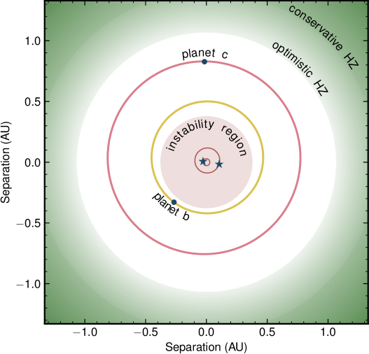
Figure 4: Overview of the TOI-1338/BEBOP-1 system along with the extent of the systems habitable zone calculated using the Multiple Star HZ website  (?). The conservative habitable zone is shown by the dark green region, while the optimistic habitable zone is shown by the light green region. Binary stars are marked by the blue stars in the centre. TOI-1338/BEBOP-1c’s orbit is shown by the red orbit models, based on $500$ randomly drawn posterior samples from a kima run, shaded from the $50^{\rm{th}}$ to $99^{\rm{th}}$ percentiles. TOI-1338/BEBOP-1b’s orbit is shown by the yellow models, and is also based on $500$ random samples drawn from the posterior in its discovery paper  (?).

Table 1: TOI-1338/BEBOP-1 system orbital parameters from our analysis of the ESPRESSO and HARPS radial velocities, after removing outliers. $1\sigma$ uncertainties are provided as the last two significant digits, within brackets. Dates are given in BJD - 2,450,000. ^∗ from Kostov et al. (2020)  (?), ^∗∗ from Triaud et al. (2017)  (?).

Binary parameters
$P_{\rm bin}$	day	14.6085579(57)
$T_{0,\rm bin}$	BJD	9287.20017(71)
$K_{1,\rm bin}$	$\rm km\,s^{-1}$	21.61764(73)
$e_{\rm bin}$	–	0.155522(29)
$\omega_{\rm bin}$	rad	2.05549(30)
$\dot{\omega}_{\rm bin}$	$\rm{arcsec\,year^{-1}}$	66.0${}^{+65.0}_{-54.7}$
$M_{1}$	$\rm M_{\odot}$	1.127(69)∗
$R_{1}$	$\rm R_{\odot}$	1.345(46)∗
$M_{2}$	$\rm M_{\odot}$	0.313(12)
$a_{\rm bin}$	$\rm AU$	0.1321(25)
$T_{\rm eff,1}$	$\rm K$	6050(80)∗
$V_{\rm mag,1}$	–	11.72(02)∗
$\rm{Spectraltype}$	–	F8∗∗
Planet b parameters
$P_{\rm b}$	day	95.174(35)∗
$K_{\rm b}$	$\rm m\,s^{-1}$	$<2.4(0.1)$
$e_{\rm b}$	–	0.0880(43) ∗
$m_{\rm b}$	$\rm M_{\oplus}$	$<21.8(0.9)$
$m_{\rm b}$	$\rm M_{Jup}$	$<0.0685(29)$
$a_{\rm b}$	$\rm AU$	0.4607(88)∗
$\rho_{\rm b}$	$\rm{g\,cm^{-3}}$	$<$0.36${}^{+0.02}_{-0.01}$
Planet c parameters
$P_{\rm c}$	day	215.5(3.3)
$T_{0,\rm c}$	BJD	9208.7(29.1)
$K_{\rm c}$	$\rm m\,s^{-1}$	5.6(1.0)
$e_{\rm c}$	–	$<$0.16
$\omega_{\rm c}$	rad	3.84(86)
$m_{\rm c}\sin i_{\rm c}$	$\rm M_{\oplus}$	65.2(11.8)
$m_{\rm c}\sin i_{\rm c}$	$\rm M_{Jup}$	0.205(37)
$a_{\rm c}$	$\rm AU$	0.794(16)
System parameters
$\gamma$	$\rm km\,s^{-1}$	30.75335(99)
Instrumental
$\rm{Jitter_{HAR}}$	$\rm m\,s^{-1}$	4.2${}^{+1.6}_{-3.0}$
$\rm{Jitter_{ESP19}}$	$\rm m\,s^{-1}$	4.2(2.0)
$\rm{Jitter_{ESP21}}$	$\rm m\,s^{-1}$	4.5(0.6)
$\rm{RV\,Offset_{ESP19}}$	$\rm m\,s^{-1}$	-146.4${}^{+1.9}_{-1.8}$
$\rm{RV\,Offset_{ESP21}}$	$\rm m\,s^{-1}$	-150.8(1.2)

Author contributions

The BEBOP project was established by DVM, and AHMJT, building on work by the WASP consortium that involved AHMJT, IB, ACC, MG, CH, PFLM, FP, AS and SU. The radial velocity (RV) data used in this manuscript were secured and obtained by MRS, AHMJT, LS, DVM, VK, DS, TAB, PFLM, NJM, and AS and their reduction involved MRS, AHMJT, FP and SU. The observational campaign was led by MRS for ESPRESSO observations, and AHMJT for HARPS. RV analysis was led by MRS with assistance from AHMJT, DVM, and JPF. Outliers in RV data were identified by TAB, and MRS. Detection limit analysis was performed by MRS, JH, and EL with help from JPF. TIP and FIP analysis was carried out by TAB, and NCH. Analysis of stellar activity was carried out by LS, MRS, and AHMJT. Independent stability analysis on the system was carried out by ACMC, and DVM with inputs from RM. Formation pathway simulations were carried out by GALC and RPN. The Transmission Spectroscopy Metric (TSM) was calculated by GD. The system was identified to have an inner transiting planet TOI-1338/BEBOP-1b by DVM, JAO and WFW. VK prepared the majority of figures in the paper. All co-authors assisted in writing and reviewing the manuscript.

Supplementary materials

Collected Observations
Modelisation of the data
Stellar Activity
System Dynamics
System Formation
Prospects for atmospheric follow-up with JWST
Journal Of Radial-Velocity Observations
Tables S1 to S4
Figures S5 to S16
References

Supporting Online Material

In this supplementary material we present additional methods and details in support of our main article “Radial-velocity discovery of a second planet in the TOI-1338/BEBOP-1 circumbinary system”. The material is organised as follows, in Section 1 we describe the collected observations for the discovery, along with outlier removal. Section 2 presents the orbital fitting and data analysis techniques utilised, along with constraints on additional planetary companions in the system. Section 3 provides an overview of the stellar activity analysis on the system. In Section 4 we discuss the stability of the system, and in Section 5 we discuss formation pathways for the planetary system. Section 6 hosts discussion on atmospheric follow-up observations of system. The Radial-Velocity data used in the analysis is available in Section 7.

1 Collected Observations

TOI-1338/BEBOP-1 was selected for the Binaries Escorted By Orbiting Planets (BEBOP) programme  (?) from a large sample of low-mass eclipsing binaries identified by the EBLM project  (?) under the name EBLM J0608-59. Those binaries were detected as part of the Wide Angle Search for Planets (WASP), as candidate transiting planet which were later shown with using radial velocities to be “false positive” eclipsing binaries. To be part of the EBLM and BEBOP sample, a system needs to be a single-lined eclipsing binary. For identification and selection, the southern sample exclusively used the CORALIE spectrograph ($R\sim 45,000$; mounted on the 1.2m Euler Swiss telescope, at La Silla, Chile). TOI-1338/BEBOP-1 was first observed as a part of the EBLM project in 2009.

The BEBOP sample represents a sub-sample of the EBLM sample, where the binaries are selected to optimise planet-finding capability. The main discriminator is the obtained radial-velocity precision, which is typically a function of magnitude. There is also a bias to wider ($\gtrsim 5$ days) binaries, since rapid rotation due to tidal locking broadens spectral lines and reduces precision. Fortunately, the Kepler results in fact show a dearth of planets transiting the tightest binaries  (?). We also progressively remove binaries where a long-term radial velocity trend reveals a presence of a third star, which is believed to have a detrimental impact on planet occurrence  (?). Finally, systems are also removed based on simple activity indicators just as the line bisector  (?). Targets within the BEBOP sample receive both longer exposures than the rest of the EBLM sample, in order to improve precision. TOI-1338/BEBOP-1 was first observed as a part of the BEBOP project in 2014. Greater details about the selection process can be found in  (?).

There exists 55 radial velocities obtained with CORALIE, which are not used in this paper. Their typical uncertainty is $25~{}\rm m\,s^{-1}$, much higher than the signal we identify. Some of them were used to determine the spin–orbit angle of the binary  (?).

1.1 HARPS

HARPS is a high-resolution, high-precision échelle spectrograph built for the detection of exoplanets  (?). It has a resolution $R\sim 100,000$ and typically achieves a long-term stability under $1~{}\rm m\,s^{-1}$. It is mounted on the ESO 3.6m telescope at La Silla, Chile.

The southern BEBOP sample, including TOI-1338/BEBOP-1 (under the name J0608-59) were observed by HARPS under two ESO large observing programmes (prog.ID 1101.C-0721 and 106.212H; PI Triaud). TOI-1338/BEBOP-1 received $61$ spectra between the dates of 2018-04-08 and 2022-04-18. Typically exposure times of 1800s were obtained, with a median radial-velocity precision of $5.73~{}\rm m\,s^{-1}$.

HARPS data were reduced by HARPS Data Reduction Software (DRS) version 3.5 (which is hosted at the Observatory of Geneva, and will be made public in a few months). A description of how the DRS works can be found in  (?) and in  (?). Spectra are correlated using a weighted numerical mask matching the spectral type of the target producing a cross-correlation function (CCF). A Gaussian function is fitted to the CCF to find the mean radial velocity.

Version 3.5 of the DRS is not very different from the version held by ESO but it allowed us to recorrelate the spectra with our own specification. The standard DRS is built to study single, slow rotating stars. It assumes two quantities: a common mean radial velocity for all spectra of a given system, and a correlation window of $30~{}\rm km\,s^{-1}$ on either side of that mean velocity. In the case of binaries, the velocity changes according to the binary phase. In addition some of the BEBOP sample targets rotate fast enough that a $30~{}\rm\,km\,s^{-1}$ window is not adequate. Using version 3.5 allowed us to centre the correlation window to the observed velocity at each epoch, thus ensuring the same set of absorption lines are used to produce the radial velocities, epoch after epoch. For TOI-1338/BEBOP-1 we used the standard $30~{}\rm km\,s^{-1}$ correlation window and a G2 mask to produce the cross-correlation window. The reduction software provides the radial velocity, its uncertainty (determined from photon noise and the line width), the line width (FWHM), the span of the bisector slope (Bis_Span), and automatically produced corrections to the barycentre of the Solar system.

All HARPS data are available at the ESO public archive by searching for J0608-59, and can be found in Table 3 in this supplementary material.

1.2 ESPRESSO

Following the discovery of TOI-1338b  (?), $20$ radial-velocity measurements were obtained in 2019 with the ESPRESSO spectrograph located in Paranal, Chile  (?) in an attempt to confirm the planet and more accurately constrain its mass (Prog.ID 103.2024, PI Triaud). Exposure times were typically $900~{}\rm s$ in length and yielded a median precision of $2.83~{}\rm m\,s^{-1}$. These data combined with previously obtained HARPS spectra yielded no detection of TOI-1338/BEBOP-1b, but hinted at the presence of an outer companion planet with an orbital period of $\approx 200$ days. To confirm this candidate planet and attempt to detect the inner transiting planet, a further $103$ ESPRESSO spectra were obtained with exposure times of $900~{}\rm s$ yielding a median precision of $2.63~{}\rm m\,s^{-1}$ (Prog.ID 106.216B PI Standing). Of these $103$ measurements, $3$ were obtained during the primary eclipse of the binary, and $1$ during the transit of planet b. These $4$ observations have been discarded from our analysis as they are affected by the Rossiter-McLaughlin effect, which we do not model here  (?, ?).

In our radial-velocity analysis, we fit for an offset between ESPRESSO data obtained in $2019$, and those in $2021$, post COVID closures. This $4.6~{}\rm m\,s^{-1}$ offset, though small, was introduced by calibration lamp change during the COVID closure of telescope in $2020$  (?). Our $2019$ dataset was obtained after the fibre change on the instrument in $2019$. Without accounting for this offset the planetary signal is still detected in the data. COVID closure of both the La Silla and Paranal observatories delayed the collection of data on this system and by consequence the discovery of this planet by a year. Complete phase coverage of TOI-1338/BEBOP-1c’s orbit was finally achieved when the final data points were collected in March $2022$.

ESPRESSO data were reduced using version 2.3.3 of the ESPRESSO pipeline (publicly available at ESO) with a procedure similar to that used to HARPS, but adapted to ESPRESSO. Each cross correlation function was obtained with a G2 template spectra, step size of $0.5~{}\rm{km\,s^{-1}}$, and a $300~{}\rm{km\,s^{-1}}$ window centered on the radial velocity of the binary. To summarise, we have $123$ ESPRESSO observations in total, with $20$ observations in ESPRESSO $2019$, and $103$ in ESPRESSO $2021/2022$. The total timespan of the HARPS and ESPRESSO combined is $1472$ days.

All ESPRESSO data are available at the ESO public archive by searching for J0608-59. All radial-velocity data used in our analysis can be found in Tables 2-4 in this supplementary material.

1.3 TESS

TOI-1338/BEBOP-1 was a target for the radial-velocity survey before the launch of TESS. It was then later discovered to contain a 95-day transiting planet (TOI-1338b, aka TOI-1338/BEBOP-1b), based on four sectors of TESS data (three in short cadence, 120 seconds). More data has been taken in the years since. These data are mentioned here for completeness but we do not include them in the analysis; TOI-1338/BEBOP-1c is an independent radial-velocity discovery.

1.4 Outlier treatment

Outliers were identified using two methods. The first involved a-priori finding outliers in the span of the bisector slope (Bis_Span, a measure of line shape  (?)) and Full Width at Half Maximum (FWHM), and excluding these data. The radial-velocity analysis in this paper used this method. The second method used a student-t distribution to account for outliers as part of the sampling process (e.g.  (?)), we used this to check the results from the first method.

Preliminary outliers were first removed where the wrong star was observed or the observations occured during an eclipse or a planetary transit. The following methods to deal with outliers were then applied to the remainder of the data.

For the a-priori removal, each set of points was fit as a mixture model with inlier and outlier populations, following the method described in Hogg et al. (2010)  (?). For both FWHM and Bis_Span, the inlier model was simply a constant with a small scatter allowed in addition to the uncertainties (which were taken as double the radial-velocity uncertainty). The outlier model also fits a constant but with a very wide population scatter.

We used PyMC3  (?) to fit a mean and scatter for both the inlier and outlier distributions, as well as a parameter $f$ for the proportion of points that are outliers, the prior on $f$ is a $\beta[1.5,9]$ distribution favouring a low proportion of outliers. These parameters were then used to calculate the probability of the $i^{th}$ point being an outlier for each posterior using the following equation:

$$P_{i,out}=\frac{fL_{i,out}}{fL_{i,out}+(1-f)L_{i,in}}$$ (1)

where $L_{i,out}$ and $L_{i,in}$ are the likelihoods for the $i^{th}$ point in the respective outlier and inlier distributions.

The power of this method is in removing the human factor from outlier identification, and not having to resort to sigma-clipping which does not usually consider measurement uncertainties. A total of 17 outliers were identified this way.

For the student-t method, we ran the fits on the dataset accounting for outliers using a student-t distribution. Outliers in radial velocity can then be directly identified, rather than relying on the Bis_Span and FWHM indicators as in method 1. This student-t method identified 6 outliers of which 3 are shared with the 17 outliers identified in method 1; the 3 points are particularly strong outliers in the student-t analysis.

Importantly, the resulting detection of TOI-1338/BEBOP-1c and non-detection of TOI-1338/BEBOP-1b is not affected by the method of dealing with outliers, and all the parameters from the student-t fit were consistent with those found removing the outliers a-priori.

In summary: 3 outliers were identified in the HARPS data in FWHM one of which is also identified in Bis_Span and is such a strong outlier it is suspected that the wrong star was observed; 1 outlier was identified in the ESPRESSO $2019$ data in FWHM; and 13 outliers are identified in the ESPRESSO $2021/2022$ data in FWHM (2 of which are also identified in Bis_Span). Data points identified as outliers are flagged in Tables 2-4 of this supplementary material. We denote outliers, excluded from the analysis, with the following flags: Wrong star W, Bis_Span B, FWHM F, During binary transit R, during planetary transit P.

2 Modeling of the data

2.1 Kima

For the radial-velocity analysis we use the kima package  (?). kima models radial-velocity data with a sum of Keplerian functions from $N_{\rm{p}}$ orbiting planets, and estimates the posterior distributions for each of the orbital parameters.

To sample the posterior distribution kima uses a Diffusive Nested Sampling (DNS) approach  (?). This provides kima with estimates on the evidence for each model, allowing for model comparison  (?, ?). This model comparison can then be used to compare the ratio of evidences between models with different numbers of Keplerian signals. Importantly, the number of planets $N_{\rm{p}}$ is a free parameter like any other.

The radial-velocity analysis follows that described in Standing et al. (2022)  (?) and Triaud et al. (2022)  (?) with added post-Keplerian corrections as described in Baycroft et al. (in prep). These corrections account for relativistic and tidal effects on the radial velocity measurements from the binary orbit which have been derived and tested in  (?, ?, ?, ?, ?). In addition, we directly fit for apsidal precession of the binary within kima, which is the largest Newtonian effect we can expect. We find a value of $\dot{\omega}_{\rm bin}=66.0^{+65.0}_{-54.7}~{}\rm{arcsec\,year^{-1}}$, distinct but barely different from zero. Details about this implementation are described in Baycroft et al. (in prep). Prior distributions used in our analysis can be found in Table 2.

Table 2: Prior distributions for the binary and planetary RV model signals in kima

Parameter	Unit	Prior distribution
		Binary	Planet
$N_{\rm p}$		$1$	$\pazocal{U}(0,3)$
$P$	days	$\pazocal{U}(14.61\pm{0.01})$	$\pazocal{LU}(4\times P_{\rm bin},2000)$
$K$	$\rm{m\,s^{-1}}$	$\pazocal{U}(21617\pm{15})$	$\pazocal{MLU}(0.1,100)$
$e$		$\pazocal{U}(0.1556\pm{0.001})$	$\pazocal{K}(0.867,3.03)$
$\phi$		$\pazocal{U}(0,2\pi)$
$\omega$		$\pazocal{U}(0,2\pi)$
$\dot{\omega}_{\rm bin}$	$\rm{arcsec\,year^{-1}}$	$\pazocal{N}(0,1000)$	-
$\sigma_{\rm jit}$	$\rm{m\,s^{-1}}$	$\pazocal{LU}(0.01,67)$
$\gamma$	$\rm{m\,s^{-1}}$	$\pazocal{U}(30761\pm{100})$

Notes: $N_{\rm p}$ denotes the Number of Planetary Keplerian signals to fit to the data. $P_{\rm bin}$ denotes the Period of the binary. $\pazocal{U}$ denotes a uniform prior with an upper and lower limit, $\pazocal{LU}$ is a log-uniform (Jeffreys) prior with upper and lower limits, $\pazocal{MLU}$ is a modified log-uniform prior with a knee and upper limit, $\pazocal{N}$ is a gaussian prior with a mean and standard deviation, and $\pazocal{K}$ is a Kumaraswamy prior  (?) which takes two shape parameters  (?).

2.2 Resulting fit

The kima combined fit of our HARPS and ESPRESSO data favours a single planet model in addition to the binary orbit with a Bayes factor of $>29,000$. The Bayes factor is the ratio of the Bayesian evidence between two competing models. In our case the Bayes factor is the number of posterior samples obtained with $\rm{N_{p}}$ planetary signals, over those with $\rm{N_{p}}-1$. The Bayes factor value indicates the measure of support in favour of one model over the other  (?, ?, ?).

A Bayes factor value of $>150$ indicates very strong evidence  (?, ?) in favour of a single planet in addition to the binary orbit.

When searching for the inner transiting planet in the data we obtain a Bayes factor of $1.4$ in favour of two planetary signals. This is categorised as inconclusive evidence of any further signals in the data.

Forcing a fit on a $95$ day Keplerian signal yields no clear signal corresponding to TOI-1338/BEBOP-1b with posterior samples having a semi-amplitude consistent with $0~{}\rm{m.s^{-1}}$. This fit still produces a clear detection of TOI-1338/BEBOP-1c.

To obtain orbital parameters for the system, we follow the same procedure as detailed in Standing et al. (2022)  (?). Proposed posterior samples with orbits which cross one another, or into the instability region of the binary, are removed. The remaining samples are clustered with the HDBSCAN clustering algorithm  (?). Clusters corresponding to the binary and TOI-1338/BEBOP-1c are then plotted using the Corner package  (?). Orbital parameters are then determined as the $50^{\rm th}$ percentile, with $1\sigma$ uncertainties estimated from the $14^{\rm th}$ and $84^{\rm th}$ percentiles of the cluster. Corner plots for the binary and TOI-1338/BEBOP-1c can be seen in Figures 5 and 6 respectively.

2.3 Constraints on TOI-1338/BEBOP-1b and further planetary companions

Using kima as in Standing et al. (2022), and Triaud et al. (2022)  (?, ?) we calculate a detection limit on additional undetected planetary signals in the radial-velocity data. Firstly, we remove the highest likelihood Keplerian model corresponding to TOI-1338/BEBOP-1c from the data. Following this, to calculate the detection limit we fix $N_{\rm{p}}=1$ in our fit, include the binary with tight priors on its parameters, and obtain posterior samples of all remaining signals which are compatible with the data. This method is conceptually similar to that described in Tuomi et al. (2014)  (?), where the sampler is forced to fit an additional signal to the data. Any signals found are compatible with the data, but as of yet undiscovered, since only one planetary signal is present in our original fit.

The resulting posterior samples can be seen as a greyscale density plot in Figure 7, with a blue $99\%$ contour corresponding to our detection limit. The blue limit demonstrates that we are sensitive to additional sub-Saturn mass planets for periods out to $2000$ days, while we are sensitive to Neptune mass planets near the instability limit.

We note a density of posterior samples at periods around $100$ days in agreement with the presence of TOI-1338/BEBOP-1b seen in TESS photometry  (?). Following the findings described in Standing et al. (2022)  (?), we calculate an additional detection limit to place an upper limit on the mass of TOI-1338/BEBOP-1b. This limit is calculated in the same manner as the blue line, though only using posterior samples with eccentricities $<0.1$ (the approximate upper limit on the eccentricity of TOI-1338/BEBOP-1b  (?), and a value allowed by our orbital stability analysis). A running mean is applied on the red eccentricity cut line to ensure $>1000$ samples are in each bin. The resulting red detection limit demonstrates our sensitivity to circular planets at the orbital period of TOI-1338/BEBOP-1b is $\approx 2.4\pm 0.1~{}\rm{m.s^{-1}}$. This allows us to place an upper limit on the mass of TOI-1338/BEBOP-1b of $21.8\pm 0.9~{}M_{\oplus}$. With a radius of $\approx 6.9~{}R_{\oplus}$, we calculate the mean density of TOI-1338/BEBOP-1b to be $<0.36~{}\rm{g.cm^{-3}}$. The mass of planet b from Kostov et al.  (?) is primarily determined thanks to the apsidal precession imprinted on the eclipse timing variations, under the assumption of a single planet. Our study uses exclusively radial velocities. Since they are not sensitive to the planet’s mass, we only place an upper limit.

The uncertainty of the detection limit is determined by performing numerical experiments with kima. We first generate a radial-velocity timeseries, following a Gaussian distribution, with dates following a log-uniform distribution. Then we run kima just like any other system and produce a large number of posteriors (in our case 685,000). Following that, we compute a detection limit like in Standing et al. (2022)  (?) and call this our fiducial case. The next step is to calculate detection limits for many subsamples of the posterior and measure their fractional distance to the fiducial detection limit. We find that the fractional error in the position of subsamples’ detection limits follows a square root law. Consequently, we fit these data with a function $y=a\,x^{-1/2}$, where $y$ is the fractional uncertainty of the detection limit at a given orbital period and $x$ is the number of posterior within a given posterior subsamples. We find $a=15.1\pm 0.3$. We use this relation to represent an uncertainty on Fig. 4.

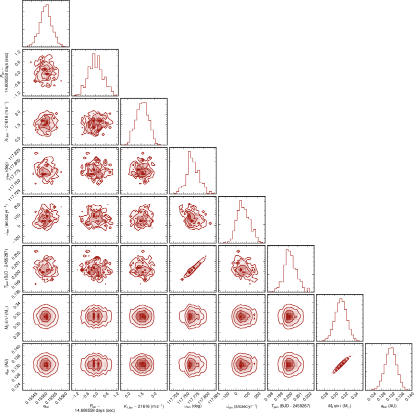
Figure 5: Corner plot of posterior sample distributions for the Binary stars orbital parameters; eccentricity, orbital period, semi-amplitude, argument of periastron, binary apsidal precession, time of periastron passage, $M\sin i$ in Solar masses, and semi-major axis.

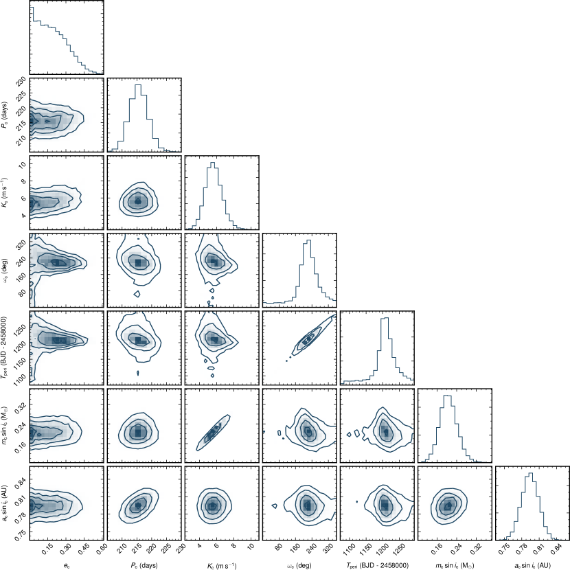
Figure 6: Corner plot of posterior sample distribution for TOI-1338/BEBOP-1c orbital parameters; eccentricity, orbital period, semi-amplitude, argument of periastron, time of periastron passage, $M\sin i$ in Earth masses, and semi-major axis.

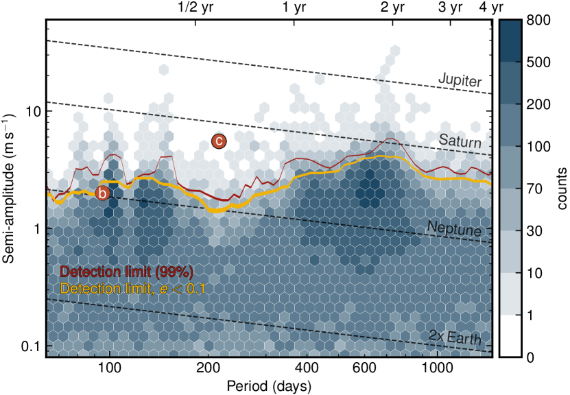
Figure 7: Hexbin plot denoting the density of $\sim 100\,000$ posterior samples obtained from four separate kima runs on TOI-1338/BEBOP-1 Radial-Velocity (RV) data with $N_{\rm{p}}$ fixed $=1$. The red line shows the calculated $99\%$ detection limit, along with its associated error. Point ‘c’ indicates the position of detected planet TOI-1338/BEBOP-1c, and point ‘b’ that of planet TOI-1338/BEBOP-1b undetected in RV data alone. The orange line shows the detection limit on samples with eccentricity $<0.1$ (the upper limit on TOI-1338/BEBOP-1b’s eccentricity  (?)).

2.3.1 FIP and TIP

We compute the True Inclusion Probability (TIP) and False Inclusion Probability (FIP) for a signal being present in the data over various frequency bins  (?). Plotting this in a periodogram gives similar information to the detection limit described above. However, where the detection limits give us information about an upper limit on the mass of a potential planetary signal, the TIP periodogram effectively gives us the probability of there being a planetary signal at that given period. It has been shown that using this metric as a detection criterion is optimal in the context of exoplanet detection  (?). We find 1 peak in the TIP periodogram further to the detected planet c at: $\approx 700$ days with TIP of 0.94. This is shown in Figure 8 which shows the FIP and TIP periodograms. We attribute this signal to the window function as seen in Figure 9, though further observations will provide greater insight into the source of the signal.

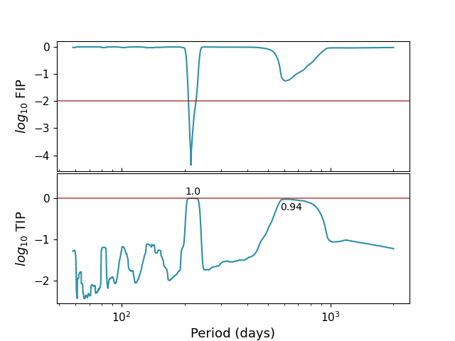
Figure 8: Top: False Inclusion Probability (FIP) periodogram showing the clear detection of TOI-1338/BEBOP-1c at $\approx 215$ days. Bottom: True Inclusion Probability (TIP) periodogram showing the significance of any other peaks with TIP $>0.2$. The second highest peak occurs at $\approx 700$ days with a significance of 94%.

3 Stellar Activity

Chromospheric emission lines observed in the stellar spectrum often trace stellar magnetic activity. Here we describe the activity indices measured and used in our analysis. We used the open-source package actin  (?) to measure the Ca II H&K, He I, sodium D doublet (Na D a and b), Ca I and H$\alpha$ activity indices.

First we compute a generalised Lomb-Scargle (GLS) periodogram  (?) of each activity indicators, from individual instruments, and using the combined dataset. In Figure 10 (a,b), we show the window function of each individual and combined datasets and the periodogram of radial velocity. We compute false alarm probability levels of $10\%$, $1\%$ and $0.1\%$ using a bootstrap randomisation of the dataset. We consider a signal to be significant if the false alarm probability level is $<0.1\%$. We searched for periodic signals of chromospheric activity indicators to investigate the possibility of TOI-1338/BEBOP-1c’s period $P_{\mathrm{c}}$ being produced by magnetic activity of TOI-1338/BEBOP-1A (the primary). Figure 10 (c-g) depicts the periodogram of Ca II, H$\alpha$, Na D, He I and Ca I indices. None of the activity indicators shows any significant signal at or near P_c ($\sim$ 215 d). We see significant period at $\sim$ 7.5 d in Na D (FAP $\sim$0.1%) and He I (FAP $\sim$1%), however, the nature of these signals are not obvious. We see weak signals in H$\alpha$ at 270 d caused by a combination of window function and a long-period term, however, the signal is not significant. In addition, the activity time series shown in Figure 11 does not show any obvious modulation.

We searched All-Sky Automated Survey (ASAS;  (?)) archival data to constraint the rotation period and to investigate the nature of the TOI-1338/BEBOP-1c signal. The ASAS observations spanning over  10 years. The ASAS data shows a strong signal at  61 d (10% false alarm probability) which could be related to stellar rotation ($\sim$3P_rot).

In addition, analysis of the radial-velocity bisector shows no correlation with the $\sim 215$ d signal, yielding a Pearson Correlation co-efficient of $<0.052$.

The ASAS data and activity indicators do not show any significant signal at $\sim 215$ d, therefore this signal is likely planetary in nature.

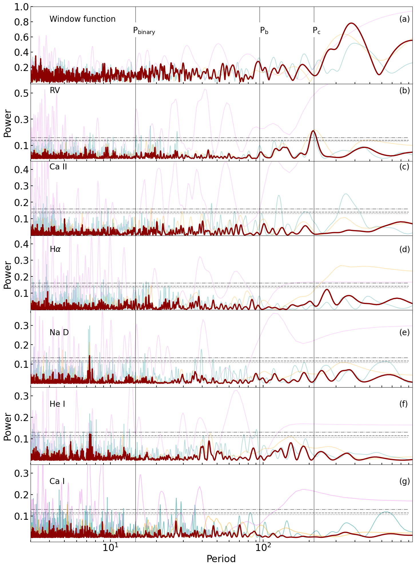
Figure 9: Generalised Lomb-Scargle periodogram of TOI-1338/BEBOP-1 spectroscopic data. The top panel shows the window function of the combined dataset (dark red). b, Periodogram of the radial-velocity measurements. c-g, Periodogram for Ca II, H$\alpha$, Na D, He I and Ca I index. The cyan, violet and orange curves corresponds to HARPS, ESPRESSO 2019 and ESPRESSO 2021/2022, respectively, and the dark red curves correspond to the combined dataset. The horizontal lines represent the bootstrapped false alarm probability levels of 10% (dotted), 1% (dashed), and 0.1% (dotted dash). The vertical solid lines indicate the binary period and planetary periods (P_b and P_c).

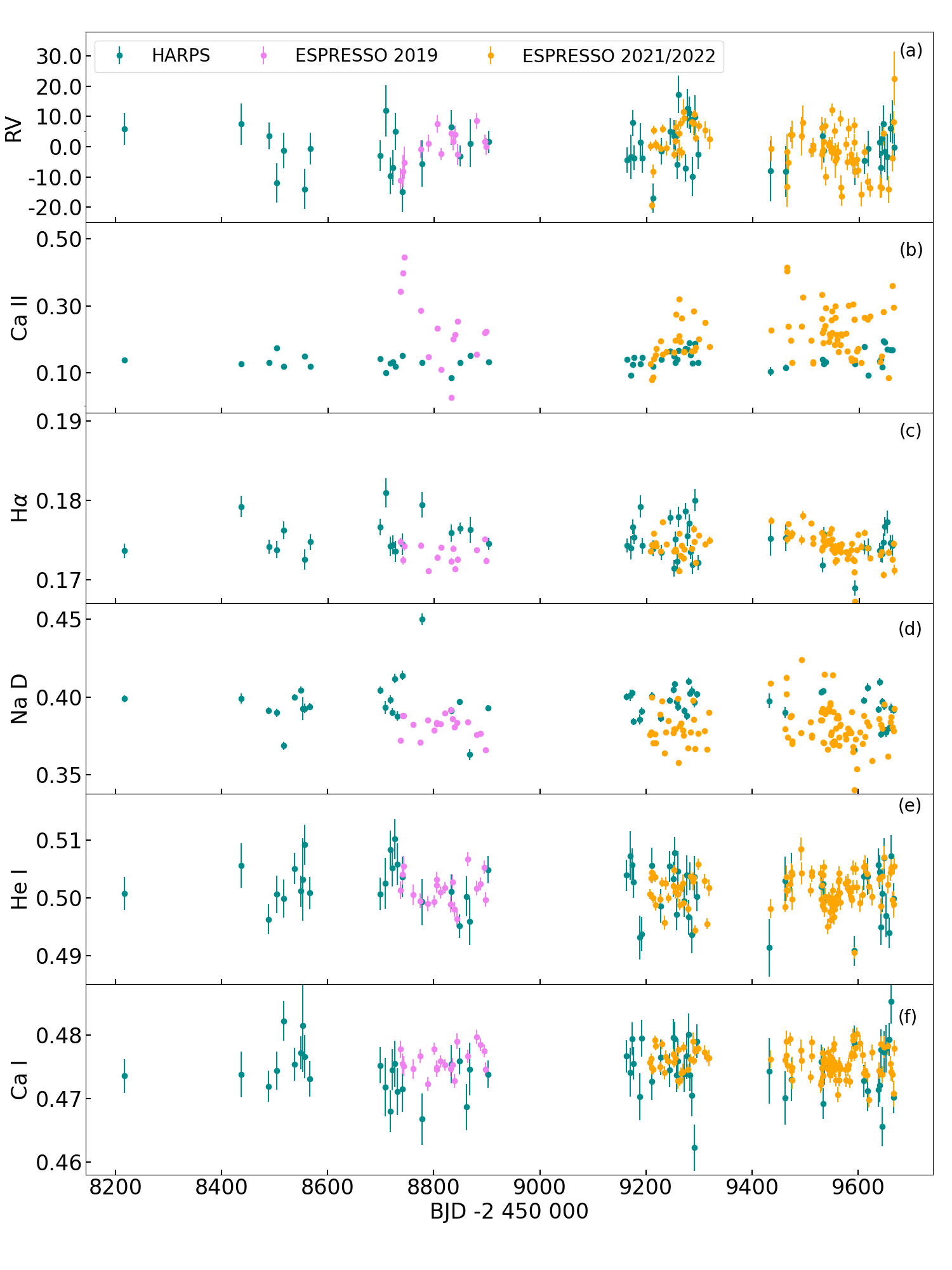
Figure 10: Radial velocity, Ca II, H$\alpha$, Na D, He I and Ca I timeseries for TOI-1338/BEBOP-1.

4 System dynamics

In this section we deal with various aspects of the orbital dynamics of TOI-1338/BEBOP-1, first looking at the stability of the system, and then estimating whether the outer planet, TOI-1338/BEBOP-1c, will show transits at some point into the future.

4.1 Orbital Stability

The orbital solution given in Table 1 in the main text shows a compact two-planet circumbinary system ($a_{\mathrm{bin}}=0.13$, $a_{\mathrm{b}}=0.46$ and $a_{\mathrm{c}}=0.79$ au). The inner planet has a maximum mass similar to Neptune ($m_{\mathrm{b}}=21.8$ M_⊕) and is close to the circumbinary stability boundary  (?, ?), while the outer planet minimum mass is similar to Saturn ($m_{\mathrm{c}}=0.21$ M_Jup). As a consequence, we expect strong mutual gravitational interactions between the stars and the planets. In order to study the stability of the system, we performed a global frequency analysis  (?, ?) in the same way as achieved for other circumbinary planetary systems  (?). In our analysis, we always consider for the inner planet its maximal mass, which can be seen as a superior limit for stability. Moreover, the mass of this planet is relatively small and does not impact much the stability, and so smaller masses do not change much the global picture described here.

The system is integrated on a regular 2D mesh of initial conditions in the vicinity of the best fit (Table 1 main text). We used the symplectic integrator SABAC4  (?), with a step size of $0.001$ yr and general relativity corrections. Each initial condition is integrated for 5000 yr, and a stability indicator, $\Delta=|1-n_{b^{\prime}}/n_{b}|$, is computed. Here, $n_{b}$ and $n_{b}^{\prime}$ are the main frequency of the mean longitude of the inner planet over 2500 yr and 5000 yr, respectively, calculated via the frequency analysis  (?). Note that while the osculating mean motion varies over a single planetary orbit as a result of energy exchange with the binary and planet c, $n_{b}$ calculated over time intervals much longer than any resonant variations is constant for stable systems, while it drifts for unstable systems until one of the planets escapes. The results are reported in color, where yellow represents strongly chaotic trajectories with $\Delta>10^{-2}$, while extremely stable systems for which $\Delta<10^{-8}$ are shown in purple/black. Orange indicates the transition between the two, with $\Delta\sim 10^{-4}$.

Observationally, only the inner planet’s eccentricity is well-constrained: $e_{\mathrm{b}}=0.088\pm 0.004$  (?). In contrast, only an upper limit can be placed for the outer, non-transiting planet: $e_{\mathrm{c}}<0.1$ (Table 1 main text).

Therefore, in a first experiment, we explore the stability of the system in the plane $(e_{\mathrm{b}},e_{\mathrm{c}})$, assuming coplanar orbits. The results are shown in Figure 11. We observe that that the eccentricities of both planets must be smaller than $0.1$ to ensure a stable system. Moreover, since we already have for the inner planet $e_{\mathrm{b}}\approx 0.1$  (?), the only remaining possibility for the outer planet is $e_{\mathrm{c}}\approx 0$. We thus adopt $e_{\mathrm{c}}=0$ in the following stability analyses.

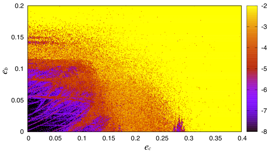
Figure 11: Stability analysis of the TOI-1338/BEBOP-1 system in the plane $(e_{\mathrm{c}},e_{\mathrm{b}})$, assuming coplanar orbits. For fixed initial conditions (Table 1 main text), the parameter space of the system is explored by varying the eccentricities of both planets, with a step size of $0.001$. For each initial condition, the system is integrated over 5000 yr and a stability indicator is calculated which involved a frequency analysis of the mean longitude of the inner planet (see text). Chaotic diffusion is indicated when the main frequency of the mean longitude varies in time. Yellow points correspond to highly unstable orbits, while purple points correspond to orbits which are likely to be stable on a billion-years timescales.

The inner planet is not detected in the radial-velocity data, its presence can only be inferred from photometric measurements  (?). Therefore, in a second experiment, we explore the stability of the inner planet orbit, by varying the orbital period and the eccentricity of this planet, assuming coplanar orbits (Figure 12). This allow us to test the compatibility of the two independent observational datasets. We observe that the inner planet lies in a small stability region that is shaped by the presence of the binary system on the left hand side and by the presence of the massive outer planet on the right hand side. We thus conclude that the two planet circumbinary solution is reliable. However, we assumed $e_{\mathrm{c}}=0$ to draw the stability map obtained in Figure 12. As we increase the eccentricity of the outer planet, the small stable region is quickly degraded and completely disappears for $e_{\mathrm{c}}>0.1$, in conformity with the results shown in Figure 11. Figure 12 shows that the inner planet, TOI-1338/BEBOP-1b, is surrounded by unstable regions. If the planet migrated to its current location, it would have to pass through two resonances with the outer planet. This could indicate consequences for formation migration in the system.

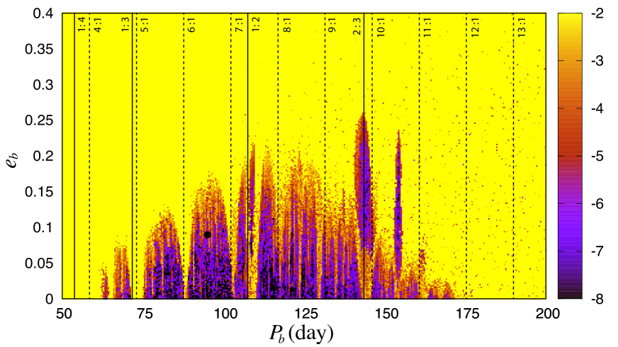
Figure 12: Stability analysis of the TOI-1338/BEBOP-1 system in the plane $(P_{\mathrm{b}},e_{\mathrm{b}})$, assuming coplanar orbits. For fixed initial conditions (Table 1 main text), the parameter space of the system is explored by varying the orbital period $P_{\mathrm{b}}$ and the eccentricity $e_{\mathrm{b}}$ of the inner planet. The step size is $0.4$ day in orbital period and $0.002$ in eccentricity. The black dot gives the best fit parameters for the inner planet  (?). The color codes are the same from Figure 11, the dashed black lines indicate resonances with the binary, and the solid black lines resonances with the outer planet TOI-1338/BEBOP-1c.

The radial-velocity technique alone is unable to constrain the inclination, $I_{\mathrm{c}}$, and the longitude of the node, $\Omega_{\mathrm{c}}$, of the outer planet. As a result, we can only determine the minimum value of its mass, which corresponds to a coplanar system ($I_{\mathrm{c}}=90$), that we have been assuming in previous analyses. However, contrarily to the inner planet, the outer planet does not transit, and thus cannot be exactly in the same orbital plane of the remaining bodies in the system. In a final experiment, we explore the stability of the system, by varying the inclination and the longitude of the node of the outer planet (Figure 13). We observe that the system can be stable within a circle centred at the coplanar solution, which corresponds to mutual inclinations smaller than $40^{\circ}$. A larger stability regions also exists centred at ($\Omega_{\mathrm{c}}=180^{\circ},I_{\mathrm{c}}=90^{\circ}$), but it corresponds to mutual inclinations higher than $120^{\circ}$, that is, to retrograde orbits, which are more unlikely from a formation point-of-view. As we change $I_{\mathrm{c}}$, the mass of the outer planet increases. At the boundary of stability, $I_{\mathrm{c}}=90^{\circ}\pm 40^{\circ}$, we get a maximum mass for the outer planet, $m_{\rm max,c}=0.28$ M_Jup. Note, however, that we can also get a mutual inclination of $40^{\circ}$ with $I_{c}=90^{\circ}$ and $\Omega_{c}=\pm 40^{\circ}$, for which the mass of the planet is on the low side, $m_{\rm min,c}=0.21$ M_Jup. Thus, the source of instability is truly mutual inclinations above the $40^{\circ}$ threshold and not masses higher than $0.28$ M_Jup. Again, we assumed $e_{\mathrm{c}}=0$ to draw the stability map obtained in Figure 12. As we increase the eccentricity of the outer planet, the radius of the stable circle quickly shrinks and completely disappears for $e_{\mathrm{c}}>0.1$, in conformity with the results shown in Figure 11.

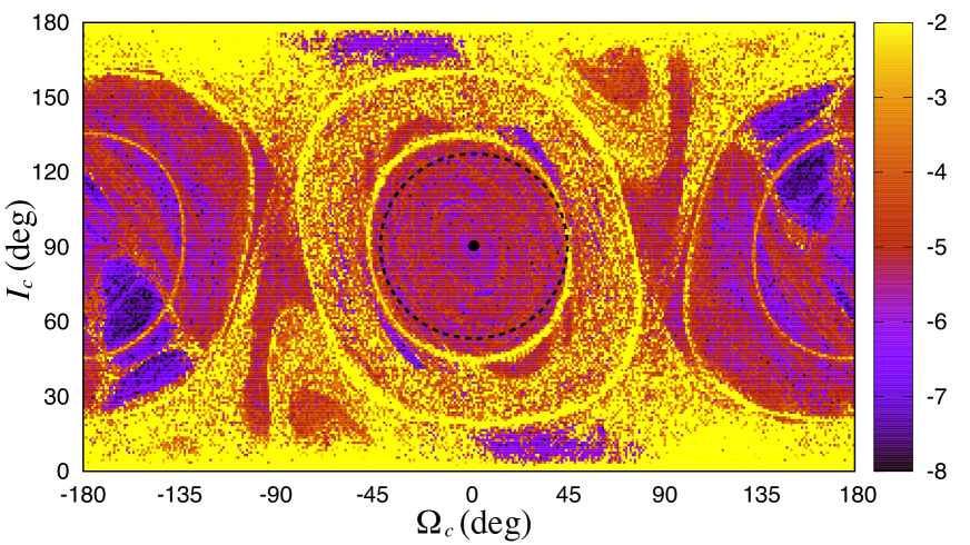
Figure 13: Stability analysis of the TOI-1338/BEBOP-1 system in the plane $(\Omega_{\mathrm{c}},I_{\mathrm{c}})$. For fixed initial conditions (Table 1 main text), the parameter space of the system is explored by varying the inclination $I_{\mathrm{c}}$ and the longitude of the node $\Omega_{\mathrm{c}}$ of the outer planet, with a step size of $1^{\circ}$. The black dot gives the best fit parameters, while the dashed circle corresponds to mutual inclinations equal to $40^{\circ}$. The color codes are the same from Figure 11.

4.2 Possible transits of TOI-1338/BEBOP-1c

Orbits of circumbinary planets exhibit nodal precession. This changes the orientation of the planet’s orbit with respect to both the binary and the observer. This means that a planet changes from a transiting to non-transiting configuration  (?, ?). The precession timescale is typically on the order of decades, and hence can be observable with long baselines such as Kepler and TESS. Kepler-413 exhibited this on-off transit sequence  (?). Kepler-453 did not start transiting until half way through the Kepler mission  (?).

(?, ?) derived an analytic criterion for if a planet will ever enter transitability on the primary (A) or secondary (B) star during its precession cycle:

$$\Delta I>\left|\frac{\pi}{2}-I_{\rm bin}\right|-\sin^{-1}\left(\frac{a_{\rm A,B}}{a_{\rm p}}\sin\left|\frac{\pi}{2}-I_{\rm bin}\right|+\frac{R_{\rm A,B}}{a_{\rm p}}\right),$$ (2)

where $\Delta I$ is the mutual inclination between the planet and binary orbit. It may seem counter-intuitive at first that a planet-binary misalignment makes transitability more likely. The reason is that the planet’s sky inclination oscillates around the binary’s sky inclination, with an amplitude equal to $\Delta I$. A higher $\Delta I$ therefore makes it more likely that the planet’s inclination will become close to $90^{\circ}$, and hence transitability. For eclipsing binaries $I_{\rm bin}$ is near $90^{\circ}$, and hence the vast majority of circumbinary planets orbiting eclipsing binaries will eventually transit.

Placing the TOI-1338/BEBOP-1c values into Eq. 2 yields $\Delta I_{\rm min}=-0.11^{\circ}$ for the primary star. The negative inclination criterion means that TOI-1338/BEBOP-1c is guaranteed to eventually transit regardless of what its mutual inclination is. This is mainly because the binary is so well-aligned with our line of sight ($I_{\rm bin}=89.658^{\circ}$) and the primary star is rather large ($R_{\rm A}=1.299R_{\odot}$). Whilst we think that TOI-1338/BEBOP-1c is guaranteed to eventually transit, we are unable to predict when and how frequently. The precession period is

$$P_{\rm prec}=P_{\rm p}\frac{16}{3}\left(\frac{a_{\rm p}}{a_{\rm bin}}\right)^{2}\frac{1}{\cos\Delta I},$$ (3)

where we assume circular orbits  (?, ?). For TOI-1338/BEBOP-1c $P_{\rm prec}=119$ years, assuming $\Delta I$ is close to zero, as is the case of the known circumbinary planets. With modern advances in medical science, there is a chance that the authors will live to see TOI-1338/BEBOP-1c transit.

5 System formation

The coplanarity between the planet and binary orbit planes for the circumbinary planets that have been discovered so far strongly suggests that these planets were formed in circumbinary protoplanetary discs that were themselves closely aligned with the binary orbit plane. We present here the results from a suite of simulations of circumbinary planet formation that were performed to examine plausible scenarios for the origin of the TOI-1338/BEBOP-1b & c system.

5.1 Circumbinary disc and N-body model

Our simulations were performed using a newly developed code designed specifically to examine the formation of circumbinary planet systems. The code employs the N-body symplectic integrator mercury6, adapted to include a central binary system  (?, ?). The code utilises the ‘close-binary’ algorithm  (?) that calculates the temporal evolution of the positions and velocities of each body in the simulations with respect to the centre of mass of the binary stars, subject to gravitational perturbations from both stars and other large bodies. The evolution of the circumbinary disc is calculated using a 1D viscous $\alpha$–disc model  (?), solving the standard diffusion equation with additional terms that account for the possible presence of a gap forming planet and a photoevaporative wind:

$$\dfrac{d\Sigma}{dt}=\frac{1}{r}\dfrac{d}{dr}\left[3r^{1/2}\dfrac{d}{dr}\left(\nu\Sigma r^{1/2}\right)-\dfrac{2\Lambda\Sigma r^{3/2}}{GM_{*}}\right]-\dfrac{d\Sigma_{\rm pe}}{dt}$$ (4)

Here, $\dfrac{d\Sigma_{\rm pe}}{dt}$ is the rate of change in surface density due the photoevaporative wind, $\Lambda$ is the torque per unit mass that operates when a planet forms and becomes massive enough to open a gap in the disc, and $\nu$ is the disc viscosity  (?), given by

$$\nu=\alpha c_{\rm s}^{2}/\Omega,$$ (5)

where $c_{\rm s}$ is the local isothermal sound speed, $\Omega=\sqrt{\frac{GM_{*}}{r^{3}}}$ is the Keplerian frequency and $\alpha$ is the viscosity parameter. The planet torque per unit mass is given by

$$\Lambda={\rm sign}(r-r_{\rm p})q^{2}\dfrac{GM_{*}}{2r}\left(\dfrac{r}{|\Delta_{\rm p}|}\right)^{4},$$ (6)

where $q$ is the planet/star mass ratio, $r_{\rm p}$ is the planet orbital radius, and $|\Delta_{\rm p}|=\max(H\text{, }|r-r_{\rm p}|)$, where $H$ is the local disc scale height. We assume that the disc is in thermal equilibrium, and as such we use an iterative method to solve the following equation  (?)

$$Q_{\rm irr,A}+Q_{\rm irr,B}+Q_{\nu}+Q_{\rm cloud}-Q_{\rm cool}=0,$$ (7)

where we balance irradiation heating from both central stars ($Q_{\rm irr,A+B}$), background heating from the residual molecular cloud ($Q_{\rm cloud}$), viscous heating ($Q_{\nu}$) with blackbody cooling ($Q_{\rm cool}$).

Mass loss due to photoevaporative winds, resulting from high-energy photons emitted by both the central stars and nearby externally located stars, occurs on a time-scale determined by the adopted flux of high energy photons  (?, ?).

Hydrodynamical simulations have shown that circumbinary discs develop precessing eccentric inner cavities, with their sizes and eccentricities being dependant on the properties of the binary and disc  (?, ?). This cavity plays an important role in the evolution of planets that migrate into its vicinity. To mimic the presence of this cavity in the 1D viscous disc model, we use a variable $\alpha$ model fitted to results from 2D hydrodynamic simulations using fargo3d  (?), that show that the mass flux through the cavity remains roughly constant within the region around the binary. For these fargo3d simulations we adopt a computational domain that spans 0.13–20 $\,{\rm au}$, and for the numerical grid we adopt a resolution of $N_{\rm r}\times N_{\rm\phi}=768\times 512$, with logarithmic radial spacing. We use the stellar parameters outlined in this work, and the disc mass lying within 40 $\,{\rm au}$ was set to equal 6% of the combined binary mass. The viscosity parameter $\alpha=10^{-3}$ and the constant disc aspect ratio was set to 0.05. To ensure the simulations reached equilibrium, we ran them for 30,000 binary orbits.

5.2 Planet migration

Planets with masses that significantly exceed a Lunar-mass undergo migration because of gravitational interactions with the surrounding disc. We follow  (?) and include Type I migration in the model via the culmination of the torque formulae that take account of Lindblad and corotation torques  (?), as well as those of eccentricity and inclination damping  (?, ?),

$$\begin{split}&\Gamma_{\rm I,tot}=F_{L}\Gamma_{\rm LR}+\left\{\Gamma_{\rm VHS}F_{p_{v}}G_{p_{v}}+\Gamma_{\rm EHS}F_{p_{v}}F_{p_{\chi}}\sqrt{G_{p_{v}}G{p_{\chi}}}+\Gamma_{\rm LVCT}(1-K_{p_{v}})\right.\\ &\left.+\Gamma_{\rm LECT}\sqrt{(1-K_{p_{v}})(1-K_{p_{\chi}})}\right\}F_{e}F_{i}\end{split}$$ (8)

where $\Gamma_{\rm LR}$, $\Gamma_{\rm VHS}$, $\Gamma_{\rm EHS}$, $\Gamma_{\rm LVCT}$ and $\Gamma_{\rm LECT}$, are the Lindblad torque, vorticity and entropy related horseshoe drag torques, and linear vorticity and entropy related corotation torques, respectively, as given by equations 3-7 in  (?). The functions $F_{p_{v}}$, $F_{p_{\chi}}$, $G_{p_{v}}$, $G_{p_{\chi}}$, $K_{p_{v}}$ and $K_{p_{\chi}}$ are related to the ratio between viscous/thermal diffusion time scales and horseshoe libration/horseshoe U-turn time scales, as given by equations 23, 30 and 31 in  (?). If a planet becomes massive enough to form a gap in the disc  (?), its migration changes from type I to type II. When transitioning from type I to type II migration the model accounts for gap formation self-consistently by calculating the torque acting on the disc due to the planet, with the back-reaction driving migration  (?). Planets in the vicinity of the inner cavity of the circumbinary disc will experience time varying forces arising from its eccentricity and precession. These are not naturally captured in a 1D disc model, so we have added additional terms to the evolution equations to incorporate these effects. Using the results from the fargo3d simulations described above, we calculate an azimuthally averaged eccentricity profile, that when used in conjunction with a uniformly precessing disc, can give the velocity of the gas in an eccentric disc at any azimuthal location. Following the calculated precession rates from previous works  (?), we assume that the disc precession rate is equal to 3,000 binary orbits. Using the steady precessing, 2D eccentric structure of the disc obtained from the hydrodynamic simulations, we created a two-dimensional map of the radial and azimuthal forces that an embedded particle at any position in the disc would feel. This map is interpolated during the N-body simulations to find the force acting on any planet that forms.

5.3 Planetary growth

The growth of planetary seeds in the model occurs via pebble accretion, and once a planet exceeds an Earth mass it starts to accrete gas from the disc. Pebble accretion models have shown that as protoplanetary discs evolve, dust coagulates into pebbles and settles in the midplane, where the pebbles drift inwards  (?). This creates a pebble production front that expands outwards over time. As the pebbles drift through the disc, they encounter planetary embryos which can accrete the pebbles with an efficiency that depends on the disc and planet properties  (?, ?). We adopt the models of  (?, ?) to account for the production of pebbles in the disc, as well as accretion onto planetary embryos. Whilst such models were derived for single stars, with no perturbing forces from a central binary, they should be sufficiently accurate for the circumbinary disc models we present here. This is because the system is a close binary, and as such once material is only $\sim$few $\,{\rm au}$ away from the central stars the gravitational force it feels is very similar to that of a single star. Given that pebble production primarily occurs far from the binary, in the outer disc regions, we assume that the formulation for single stars is accurate. In terms of planets accreting pebbles, the same applies with most planets accreting pebbles at distances greater than $2\,{\rm au}$. However, some planets are able to migrate and accrete pebbles near the cavity, and here it would not be suitable to assume that the pebbles follow circular Keplerian orbits. Results from previous work have shown that dust particles with small Stokes numbers closely follows the gas  (?), and as such we assume that the pebbles follow the same eccentric profiles as used to calculate the torques acting on the planet in the vicinity of the central cavity. The relative velocities between pebbles drifting past the planet are then calculated and used in the equations for pebble accretion  (?).

Gas accretion onto the planets is modelled using a recently developed empirical fit  (?) to the results of detailed 1D envelope structure models  (?) that account for local disc conditions:

$$\left(\dfrac{dM_{\mathrm{ge}}}{dt}\right)_{\mathrm{local}}= 10^{-10.199}\left(\dfrac{\mathrm{M_{\oplus}}}{\mathrm{yr}}\right)f_{\mathrm{opa}}^{-0.963}\left(\dfrac{T_{\mathrm{local}}}{\mathrm{1\,K}}\right)^{-0.7049}\left(\dfrac{M_{\mathrm{core}}}{\mathrm{M}_{\oplus}}\right)^{5.6549}\left(\dfrac{M_{\mathrm{ge}}}{\mathrm{M}_{\oplus}}\right)^{-1.159}$$

$$\times\left[\exp{\left(\dfrac{M_{\mathrm{ge}}}{M_{\mathrm{core}}}\right)}\right]^{3.6334}.$$ (9)

where $T_{\rm local}$ is the local disc temperature, $f_{\rm opa}$ is an opacity reduction factor, equal in this work to 0.01, and $M_{\rm core}$ and $M_{\rm ge}$ are the planet’s core and envelope masses respectively. Given that these models calculate orbit averaged accretion rates, we assume this is also valid for planets in eccentric circumbinary discs, however further work examining the validity of this assumption should be undertaken. We note these models predict that gas accretion starts off very slowly and speeds up as the core and envelope grow in mass. Hence, the onset of gas accretion does not generally result in the formation of a gas giant planet because the envelope contracts on its Kelvin-Helmholtz time-scale.

5.4 The resulting circumbinary planet systems

The simulations were initiated by placing 42 planetary seeds throughout the disc between 2 and 20 au, with eccentricities and inclinations distributed uniformly up to $e=0.02$ and $i=0.5^{\circ}$, respectively. The initial masses of the seeds were set to equal one tenth of the transition mass, which is where pebble accretion becomes efficient as the planetary core begins to accrete from the entirety of its Hill sphere as opposed to its Bondi sphere. These initial masses were between $10^{-4}$ and $10^{-3}M_{\oplus}$ and are consistent with recent simulations of planetary embryo formation within protoplanetary discs based on gravitational collapse  (?). We initialised the gas surface density according to $\Sigma=\Sigma_{0}\left(\frac{r}{1\,{\rm au}}\right)^{-1}$ where $\Sigma_{0}$ depends on the initial disc mass. We explored discs masses between 10–15% of the combined stellar mass in discs that extend out to 100$\,{\rm au}$, and we considered metallicities of 0.5, 1 or 2 $\times$ the Solar value. We assumed a viscous $\alpha$ of $2\times 10^{-3}$, an $f_{41}$ parameter for EUV photoevaporation of 100, and an external photoevaporative mass loss rate for a disc of size 100$\,{\rm au}$ of $3\times 10^{-7}\,{\rm M}_{\odot}\,{\rm yr^{-1}}$.

Figure 14 shows the mass and semimajor axis evolution from an example simulation that formed a planetary system similar to TOI-1338/BEBOP-1. Black points show the final masses and semimajor axes of the surviving planets, whilst the vertical black dashed line denotes the stability boundary  (?). The red triangle and plus sign indicate the locations of TOI-1338/BEBOP-1b and c.

The formation of this system occurred as follows. As the pebble front moved outwards, the planetary embryos on the most circular orbits were able to accrete pebbles efficiently, allowing a number of them to grow to masses greater than an Earth mass. These planets began to migrate, generally in towards the central cavity, and continued to accrete drifting pebbles as well as gas. The central cavity in the disc provides a positive surface density gradient in the gas, and this allowed corotation torques to balance Lindblad torques for planets arriving there, resulting in migration stalling. Hence, inward migrating planets started to congregate near the outer edge of the cavity, with some resonant chains forming. As the planets continued to grow in mass, two planets with masses $\sim 10M_{\oplus}$ collided, forming a more massive core. This planet was then able to accrete gas more efficiently and entered a brief period of runaway gas accretion to become a gas giant. As the planet’s mass increased, it migrated in closer towards the central stars, pushing planets interior to it into the cavity, and closer to the stability boundary. This resulted in the inner-most planets being ejected from the system as they crossed the stability boundary and were gravitationally scattered by the central stars, although the planet destined to become the TOI-1338/BEBOP-1b analogue remained outside of the boundary. The gas giant planet opened a gap in the disc and began to undergo slow inwards type II migration, whilst continuing to accrete gas through the gap at the viscous supply rate. After 1.8 Myr the disc reached the end of its life and was fully dispersed due to photoevaporative winds, and the giant planet stopped accreting and migrating, leaving both planets with masses and semimajor axes similar to those inferred from the observations. The system was allowed to evolve for a further 8 Myr, during which time it remained stable, yielding the final system shown in figure 14.

This evolution scenario was a common outcome for a number of simulated systems, with planets growing through pebble accretion at large radii in the disc, before migrating in towards the central cavity. Planets congregated there, leading to collisions and some ejections. Figure 15 shows the mass versus semimajor axis for all planets formed in the simulations, with the colour coding showing the metallicity of the system in comparison with the Solar value (this determines the mass in pebbles assumed in the models). Planets shown by grey points have been lost from the systems through collisions with more massive planets or by ejection. The black dashed line shows the stability boundary, whilst the black triangle and plus sign show the masses and locations of TOI-1338/BEBOP-1b and c.

The figure shows that formation of TOI-1338/BEBOP-1b analogues is a relatively common outcome of the simulations, with numerous super-Earth and Neptune mass planets being formed with similar orbital periods. This is unsurprising given that these planets become trapped relatively easily around the cavity, close to the observed location of TOI-1338/BEBOP-1b. For TOI-1338/BEBOP-1c, this planet has fewer simulated planets in its proximity, a result of its observed mass. At this mass, planets are in a runaway gas accretion regime, where they quickly grow to masses greater than Saturn’s. Indeed, in our best fit simulation, the gas giant planet had a mass roughly twice that inferred for TOI-1338/BEBOP-1c. In our best fitting simulations, runaway gas accretion was initiated close to the end of the disc lifetimes, which limited the amount of gas that could be accreted by the planets. This necessity for appropriate timing could indicate that TOI-1338/BEBOP-1c formed very late in the disc lifetime.

Looking at the metallicities required to form the planets, no systems with half the Solar metallicity were able to form systems similar to TOI-1338/BEBOP-1. This was because cores with sufficient mass to undergo efficient gas accretion were unable to form. On the other hand, systems with twice the Solar metallicity were too effective at forming massive cores, resulting in too many gas giant planets forming, and few planets with masses comparable to TOI-1338/BEBOP-1b remaining in the system, making them poor fits for comparison. These results show that the metallicity of the system, and how efficiently dust is converted into planets, is important for determining the architectures of circumbinary planet systems.

Finally, we note that the orbital configuration of TOI-1338/BEBOP-1, with planet periods of 95 and 215 days and the more massive planet on the outside, is consistent with the prediction of Fitzmaurice et al. (2022)  (?) in their study of migrating multi-planet circumbinary systems. They predict that if there is a planet near the stability limit, as is the case for TOI-1338/BEBOP-1, then any equal or more massive outer planets would be located on a period more than double that of the inner planet. Their simulations show that if an exterior planet carrying greater angular momentum reaches the 2:1 resonance with the inner planet, the two lock into resonance and the inner planet is pushed into the inner cavity, resulting in ejection. The periods in TOI-1338/BEBOP-1 at 95 and 215 days are explained by the disc dissipating (and hence stopping migration) before the outer planet reaches the 2:1 resonance.

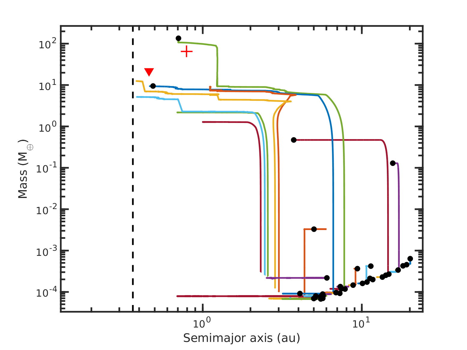
Figure 14: Evolution of the mass versus semimajor axes for the best matching simulated planetary system formed through pebble accretion to TOI-1338/BEBOP-1. Black dots represent the final masses and locations of the planets, whilst the red triangle and plus show the observed locations of TOI-1338/BEBOP-1b and c respectively. The black dashed line denotes the stability limit for the system  (?).

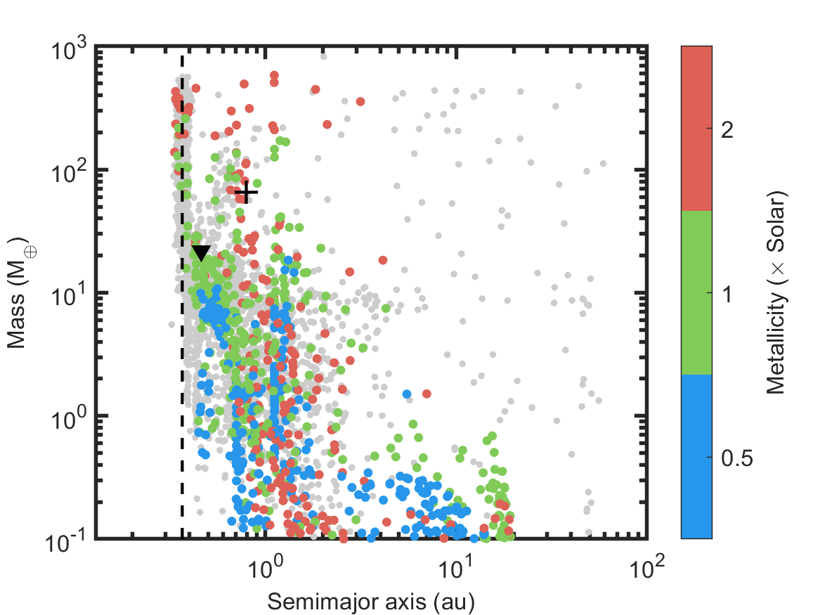
Figure 15: A mass versus semimajor axes plot showing all planets formed in simulations. Different colour points show the initial metallicity of the sytems, whilst the grey points show planets there were lost, either through accretion into other planets, or ejection from the system. TOI-1338/BEBOP-1b and 1c are denoted by the black triangle and plus symbols. The black dashed line denotes the stability limit for the system  (?).

6 Prospects for atmospheric follow-up with JWST

In order to assess the suitability of TOI-1338/BEBOP-1b for atmospheric characterisation using transmission spectroscopy, we calculate its Transmission Spectroscopy Metric (TSM) as established by Kempton et. al. (2018)  (?). A planet’s TSM is proportional to the SNR that could be achieved by observations using JWST, and it depends on the planet’s mass, radius and equilibrium temperature, and the host star’s radius and J-band magnitude.

Calculation of TOI-1338/BEBOP-1b’s equilibrium temperature is non-trivial; its non-zero eccentricity and changing irradiation levels caused by the binary mean that the temperature oscillates between minimum and maximum values. Full modelling of this, as was done in Kane & Hinkel (2013)  (?), is beyond the scope of this paper, so we estimate a mean equilibrium temperature based on two extremes: when the secondary star is closest and furthest to the planet. The equilibrium temperature calculated from the irradiation of just the primary star is $\rm 501\,K$, and the motion of the secondary star will cause the true equilibrium temperature to vary between $\rm 603-659\,K$.

We calculate the TSM following Kempton et al. (2018)  (?) using a mean $\rm T_{eq}=630\,K$ and the mass upper limit of $\rm M_{b}\,<\,21.8\,M_{\oplus}$ in the first instance, yielding a TSM of 39. This value is below the suggested JWST cut-off of 96 for planets in the sub-Jovian regime. However, the mass used for this calculation is the upper limit; a lower mass would imply a larger scale height and therefore a significantly larger TSM.

In Figure 16 we present the TSM of TOI-1338/BEBOP-1b as compared to other known exoplanets. Its position shows that even the lower limit of its TSM range compares favourably with other sub-Jovian sized planets in its temperature regime. We have indicated with an arrow the range of TSMs possible for a mass down to $\rm 10\,M_{\oplus}$, which would imply a mean density of $\rm 0.17\,g/cm^{3}$, comparable to Kepler-47c, for example  (?).

We also note that crucially, of the now 15 known circumbinary exoplanets, TOI-1338/BEBOP-1b is the only one for which observations of this kind can currently be pursued. Most Kepler systems are too faint (e.g. Kepler-47 with a $\rm Jmag=13.970$  (?), or Kepler-34 with a $\rm Jmag=13.605$  (?)), and others such as Kepler-16 no longer transit  (?). Therefore, despite the challenges it may present, TOI-1338/BEBOP-1b is our only possibility to shed light on the atmospheric make-up of circumbinary planets.

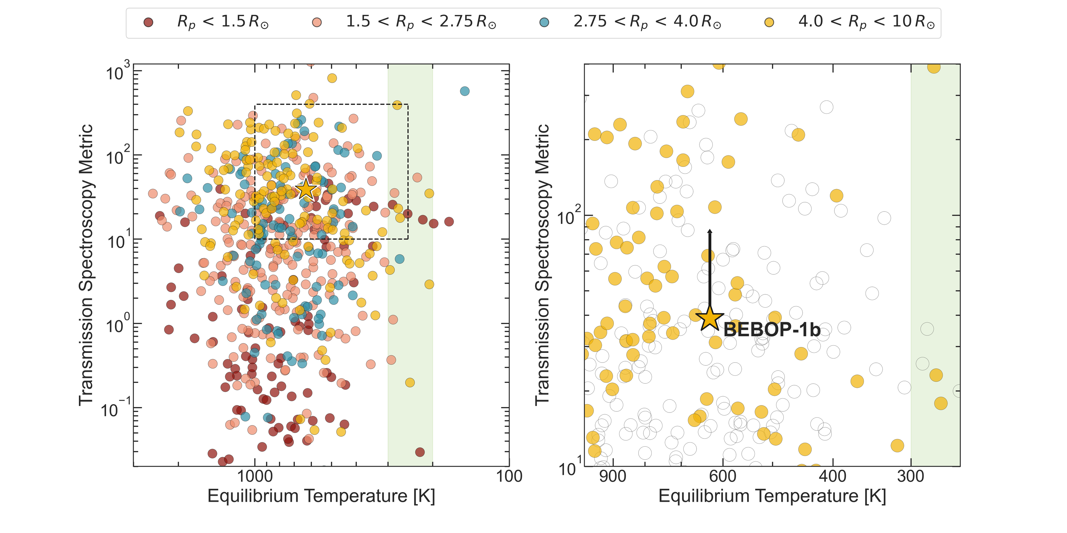
Figure 16: Transmission spectroscopy metric as a function of equilibrium temperature for planets with measured masses. Planets are coloured according to their size range, with TOI-1338/BEBOP-1b plotted as a yellow star as it falls into the sub-Jovian regime of $\rm 4.0<R_{p}<10~{}R_{\oplus}$. In both panels we show in light green the position of the temperate zone between $\rm 200-300~{}K$. In the right hand panel we zoom in on the vicinity of TOI-1338/BEBOP-1b and indicate with a black arrow the range of possible TSMs for a mass down to $\rm 10~{}M_{\oplus}$. Data for this plot was retrieved from the NASA Exoplanet Archive  (?) on May 18th 2022.

7 Journal Of Radial-Velocity Observations

Table 3: Journal of Observations containing our HARPS data for TOI-1338/BEBOP-1. Flags indicate whether the measurement is identified as a potential outlier for the following reasons: W, wrong star; B, bisector outlier; F, FWHM outlier; R, during binary transit; P, during planetary transit; S, identified by student-t. Dates are given in BJD - 2,400,000. $V_{\rm rad}$ are the measured radial velocities with their uncertainties $\sigma_{V_{\rm rad}}$. FWHM is the Full With at Half Maximum of the Gaussian fitted to the cross correlation function, and contrast is its amplitude. Bis. span is the span of the bisector slope. Uncertainties on FWHM and bis. span are $2\times\sigma_{V_{\rm rad}}$.

flag	BJD-2,400,000	$V_{\rm rad}$	$\sigma_{V_{\rm rad}}$	FWHM	contrast	bis. span
	[days]	[$\rm km\,s^{-1}$]	[$\rm km\,s^{-1}$]	[$\rm km\,s^{-1}$]		[$\rm km\,s^{-1}$]
	58216.529441	50.78673	0.00527	8.62517	33.284	0.04984
	58436.821943	48.95425	0.00683	8.60645	33.510	0.01450
	58488.758689	23.57766	0.00433	8.61047	33.532	0.02913
	58503.731900	26.22766	0.00648	8.62748	32.803	0.04815
	58516.712301	14.71036	0.00592	8.62249	33.393	0.03321
	58556.646009	20.57355	0.00664	8.61148	33.356	0.02785
	58566.604454	50.14641	0.00526	8.65706	33.177	0.06616
	58698.935537	50.75479	0.00501	8.63891	33.166	0.04375
	58708.900586	30.92087	0.00844	8.62618	33.307	0.03230
	58717.869356	14.86234	0.00608	8.64292	33.309	0.03386
	58721.884268	19.14344	0.00577	8.63451	33.503	0.03270
	58726.880800	49.14747	0.00606	8.63034	33.580	0.02617
	58740.815851	46.73639	0.00673	8.65363	33.015	0.02828
	58777.865197	7.57447	0.00775	8.62193	33.480	0.04777
	58832.810367	37.48155	0.00573	8.63670	33.207	0.03620
	58848.722188	21.71885	0.00350	8.64730	33.414	0.02062
F	58861.667840	41.08977	0.00616	8.55803	33.640	0.03357
	58867.644660	16.88223	0.00783	8.64317	33.465	0.02665
	58902.582483	50.11217	0.00377	8.60631	33.474	0.04012
	59163.705508	43.13564	0.00417	8.60739	33.669	0.04133
	59170.792366	14.32580	0.00741	8.59433	33.516	0.02690
	59173.721395	12.42927	0.00439	8.61091	33.624	0.02420
	59176.668061	32.95458	0.00417	8.61199	33.595	0.01304
	59188.634700	14.25913	0.00636	8.62851	33.702	0.04388
	59191.651879	35.49221	0.00486	8.59691	33.561	0.02025
	59211.662441	45.90963	0.00487	8.61660	33.531	0.04283
	59227.640383	32.91789	0.00448	8.61194	33.672	0.03462
	59244.662941	8.79879	0.00444	8.64343	33.221	0.01978
	59251.644571	44.61290	0.00520	8.63634	33.503	0.02609
	59254.602429	49.90968	0.00448	8.63231	33.600	0.03055
	59257.658434	22.97524	0.00496	8.62586	33.461	0.02828
	59260.590560	8.80567	0.00614	8.63341	33.413	0.06138
	59272.597942	19.04391	0.00456	8.61572	33.388	0.02352
	59276.545689	15.95709	0.00645	8.65730	33.152	0.05425
	59280.570701	43.13379	0.00535	8.65045	33.420	0.05059
	59282.587090	50.43272	0.00429	8.66531	33.226	0.03972
	59286.640886	25.88951	0.00658	8.61449	33.288	0.04448
	59291.599947	19.03116	0.00717	8.67435	32.989	0.01348
	59296.574262	49.02190	0.00485	8.65725	33.296	0.05447
	59432.915546	23.53480	0.01006	8.60847	33.470	-0.00621
	59461.840683	27.18387	0.00837	8.63513	33.182	0.02817
F	59474.875056	44.09898	0.00608	8.55833	33.404	0.05304
	59530.787352	50.18431	0.00435	8.59874	33.507	0.04165
	59533.768571	40.07132	0.00398	8.59069	33.524	0.03166
W/S	59536.865577	8.58978	0.00536	8.78151	32.610	-0.05729
	59592.644734	35.36664	0.00442	8.58328	33.543	0.02524
	59610.628629	7.60999	0.00424	8.60636	33.508	0.03719
	59617.633579	47.93738	0.00585	8.62591	33.392	0.04730
	59638.669783	11.07926	0.00542	8.61874	33.062	0.02959
	59640.662829	9.73189	0.00551	8.62356	33.143	0.02188
	59643.549232	28.77716	0.00566	8.60709	33.489	0.04687
	59645.617218	42.22367	0.00624	8.62776	32.944	0.05350
	59648.619602	50.65155	0.00662	8.64878	32.875	0.01530
	59652.605979	17.00512	0.00764	8.58887	32.870	0.03801
	59658.559334	31.63510	0.00474	8.60176	33.121	0.01684
	59662.578359	50.64357	0.00709	8.61825	32.884	0.04475
	59666.562593	24.65893	0.00460	8.62847	33.322	0.02856
	59678.558881	48.91383	0.00613	8.63485	33.275	0.04387
	59682.528521	10.85815	0.00699	8.61124	33.206	0.07145
	59686.540476	22.71545	0.00689	8.60983	32.928	0.05059
	59688.495789	36.51633	0.00633	8.61060	33.306	0.04156

Table 4: Journal of Observations containing our 2019 ESPRESSO data for TOI-1338/BEBOP-1 pre-calibration lamp change. Flags indicate whether the measurement is identified as a potential outlier for the following reasons: W, wrong star; B, bisector outlier; F, FWHM outlier; R, during binary transit; P, during planetary transit; S, identified by student-t. Columns are as in Table 3.

flag	BJD-2,400,000	$V_{\rm rad}$	$\sigma_{V_{\rm rad}}$	FWHM	contrast	bis. span
	[days]	[$\rm km\,s^{-1}$]	[$\rm km\,s^{-1}$]	[$\rm km\,s^{-1}$]		[$\rm km\,s^{-1}$]
	58736.877282	21.76153	0.00386	9.35270	45.08543	-0.02995
	58740.853942	46.75387	0.00508	9.37866	43.97280	-0.02901
	58743.882022	47.54869	0.00525	9.34604	44.67442	-0.02851
F	58760.868104	24.05023	0.00525	9.40855	44.55251	-0.00934
	58774.797532	32.50228	0.00288	9.36375	45.12590	-0.00107
	58788.804499	39.20782	0.00281	9.35552	46.13411	-0.01414
	58800.687988	50.49684	0.00211	9.33485	46.21587	0.00094
	58805.840799	11.96096	0.00293	9.34411	46.18027	-0.02645
	58805.853819	11.86026	0.00276	9.32303	46.18795	-0.02347
	58812.832857	41.52667	0.00202	9.34686	46.40748	-0.00833
	58820.719656	10.11904	0.00191	9.33895	46.26380	-0.01669
	58831.662527	46.86291	0.00312	9.34385	45.91930	-0.00895
	58835.596434	8.75913	0.00302	9.35211	45.82418	-0.03332
	58839.611578	25.24170	0.00281	9.34291	45.97437	0.00664
	58843.641422	48.67236	0.00338	9.36552	45.89060	-0.03628
	58864.576277	9.94548	0.00245	9.33974	46.43191	-0.03564
	58880.582185	8.10059	0.00260	9.36042	46.02511	-0.03986
	58887.547492	48.91687	0.00226	9.34008	46.16192	-0.03410
	58895.570898	9.36537	0.00245	9.35557	45.63188	-0.02719
	58897.568595	21.74950	0.00285	9.33254	45.99687	-0.00162

Table 5: Journal of Observations containing our 2021/22 ESPRESSO data for TOI-1338/BEBOP-1 post-calibration lamp change. Flags indicate whether the measurement is identified as a potential outlier for the following reasons: W, wrong star; B, bisector outlier; F, FWHM outlier; R, during binary transit; P, during planetary transit; S, identified by student-t. Columns are as in Table 3.

flag	BJD-2,400,000	$V_{\rm rad}$	$\sigma_{V_{\rm rad}}$	FWHM	contrast	bis. span
	[days]	[$\rm km\,s^{-1}$]	[$\rm km\,s^{-1}$]	[$\rm km\,s^{-1}$]		[$\rm km\,s^{-1}$]
	59207.687480	43.80224	0.00156	9.37761	46.31836	-0.01166
S	59209.628417	50.37108	0.00159	9.37580	46.43171	-0.02890
	59211.660755	45.77950	0.00217	9.35553	46.17093	-0.03101
	59213.608767	25.62042	0.00147	9.35216	45.85679	-0.01713
	59216.617681	8.18971	0.00153	9.37519	46.34949	-0.03437
	59218.740865	20.18316	0.00159	9.36935	46.11973	-0.01806
	59226.586386	43.49514	0.00155	9.36541	46.26637	-0.03917
	59230.661220	7.43254	0.00144	9.36048	46.40324	-0.04251
F	59234.763082	30.43838	0.00253	9.38958	45.42103	-0.02132
	59237.675552	47.27860	0.00239	9.38360	45.80074	-0.01717
R	59242.594322	28.37619	0.00158	9.35821	46.07464	0.02823
	59251.647333	44.47071	0.00156	9.36148	46.26004	-0.00822
	59253.579655	50.52710	0.00157	9.36675	46.24797	-0.02805
	59255.616689	44.90922	0.00231	9.36382	45.55454	-0.01475
	59260.656954	8.86909	0.00349	9.38242	45.03587	-0.02082
	59261.570641	13.44921	0.00147	9.36278	46.13836	-0.01415
	59263.543084	27.30447	0.00174	9.35886	46.22777	-0.02054
	59265.633180	41.15591	0.00192	9.37520	45.80166	-0.03367
	59269.686062	48.06284	0.00402	9.36591	45.33246	-0.02726
	59270.617600	41.76652	0.00167	9.36544	46.13202	-0.00691
	59279.615948	37.38595	0.00148	9.32690	46.62544	-0.02920
	59284.600155	46.44112	0.00154	9.37661	46.35578	-0.00420
	59288.601602	8.24637	0.00393	9.39004	45.29095	-0.01497
	59289.558302	7.94851	0.00140	9.36444	46.36742	-0.01240
	59292.617105	26.25967	0.00160	9.36279	46.38443	-0.01914
	59298.529197	49.47896	0.00180	9.36071	46.01858	-0.01272
	59310.557405	46.63806	0.00277	9.35520	45.72558	0.01329
R	59315.529230	30.05916	0.00161	9.22765	46.59440	-0.01299
	59318.493789	7.49658	0.00334	9.37612	46.25952	0.00924
	59434.886191	7.72835	0.00406	9.38789	45.20792	-0.02862
	59461.875388	26.60478	0.00179	9.38405	46.00120	-0.00395
F	59464.797631	7.78951	0.00610	9.38198	44.24505	-0.03947
	59464.852082	7.91591	0.00562	9.43539	44.26999	-0.00213
	59466.891173	18.78338	0.00248	9.33472	45.93830	-0.02929
	59471.888348	48.91225	0.00257	9.35499	46.10455	-0.00382
	59473.770470	49.65291	0.00441	9.37446	45.85213	-0.02673
F	59475.781757	35.16473	0.00544	9.40688	44.61897	-0.03005
F	59475.793768	35.03023	0.00471	9.40944	45.39922	-0.02857
	59491.728251	18.88142	0.00603	9.31472	46.12284	-0.07435
	59493.720410	7.44845	0.00559	9.35603	45.28000	-0.04729
	59509.854678	13.07129	0.00236	9.34211	46.23157	-0.02061
	59512.842954	34.02253	0.00245	9.35205	46.87258	-0.00193
	59512.855927	34.11283	0.00263	9.35547	46.69308	-0.00158
	59529.677831	46.60567	0.00361	9.32951	45.79053	-0.02134
F	59530.618883	49.68125	0.00494	9.40343	44.94001	-0.02776
	59531.802019	50.44588	0.00226	9.33524	46.23785	-0.03232
	59532.720289	47.66931	0.00204	9.33130	46.39628	-0.01964
	59533.679007	40.78062	0.00228	9.34486	46.03277	-0.00715
R	59534.615899	30.40381	0.00337	9.35282	45.33094	0.01244
	59535.766807	16.55441	0.00255	9.34206	45.89073	-0.03407
F	59536.619244	9.64249	0.00294	9.41335	45.01306	-0.03384
F/S	59537.738391	7.59953	0.00371	9.41515	46.07402	-0.03767
	59542.613295	37.64360	0.00311	9.37607	45.61895	-0.04708
	59543.758054	44.17420	0.00190	9.33951	46.37724	-0.02434
	59544.665713	48.05618	0.00205	9.34654	46.12688	-0.01813
	59545.669437	50.44361	0.00231	9.35663	46.08663	-0.04244
	59546.842367	49.57590	0.00287	9.32741	46.09767	-0.03066
	59547.702845	45.48948	0.00291	9.36807	45.72661	-0.01271
	59548.622872	37.39873	0.00351	9.38229	45.23370	0.00187
	59549.670272	24.81471	0.00212	9.34777	45.99796	-0.00368
	59550.722645	13.21611	0.00169	9.32627	46.16202	-0.00265
	59551.671532	7.91486	0.00293	9.35368	45.91887	0.03150
	59552.697168	8.43029	0.00194	9.33663	46.34639	-0.00803
	59553.676730	13.05334	0.00250	9.34812	46.18860	-0.02586
	59554.576962	19.02977	0.00331	9.36551	45.58520	-0.02356
	59555.605078	26.50216	0.00557	9.37734	45.04094	-0.06264
	59557.592836	39.92466	0.00235	9.35799	45.96443	-0.03400
	59558.690961	45.71291	0.00203	9.33884	46.20128	-0.02282
	59561.597912	49.09863	0.00317	9.37203	46.28033	-0.02749
F	59562.588878	43.45288	0.00405	9.40179	46.07450	-0.00592
	59563.570834	33.56211	0.00269	9.37255	46.56322	0.00182
	59564.605166	20.81757	0.00255	9.35978	46.22947	-0.01380
F/S	59565.620260	10.95610	0.00398	9.39488	45.62137	-0.05093
B/F	59566.626009	7.41922	0.00318	9.39870	45.77566	-0.05742
	59575.684564	50.37154	0.00214	9.34620	46.22991	-0.02944
	59577.752093	38.32622	0.00270	9.37025	45.73892	-0.00015
	59580.674743	8.59139	0.00317	9.35019	45.25616	-0.02305
	59582.578623	11.25863	0.00264	9.33852	45.84375	-0.01116
	59584.601711	24.89331	0.00227	9.34412	46.15903	-0.00402
	59586.580398	38.52810	0.00200	9.34233	46.24767	-0.01804
	59588.561475	48.28672	0.00347	9.35869	45.42404	0.00701
	59590.718141	49.42114	0.00288	9.37818	45.52608	0.00617
	59590.763503	49.27649	0.00257	9.34866	45.75520	-0.03599
	59592.683281	34.77366	0.00219	9.34450	46.11654	-0.01601
	59595.638420	7.62069	0.00233	9.36676	46.04454	-0.05363
	59597.574782	13.47948	0.00244	9.34960	45.45612	-0.00326
F	59603.794993	49.94906	0.00394	9.40307	44.85825	-0.00935
B/F/S	59607.733856	29.58589	0.00438	9.43764	44.46652	-0.07771
	59610.557055	7.43040	0.00243	9.37618	45.63957	-0.00768
P	59613.678124	23.84446	0.00488	9.35368	45.36720	0.00387
	59616.558505	42.91328	0.00269	9.37147	45.71280	-0.01982
	59620.543282	46.73256	0.00303	9.33914	45.78754	0.02492
	59626.642810	12.57945	0.00368	9.33877	45.58173	-0.01760
	59639.611804	7.44974	0.00384	9.36696	45.70465	-0.01814
	59642.523956	21.14343	0.00325	9.35484	45.06757	-0.03741
	59645.600842	41.97985	0.00386	9.35632	46.48695	0.00010
S	59648.534020	50.54759	0.00650	9.36679	46.66851	-0.06742
	59655.659961	11.45834	0.00449	9.35032	46.25790	-0.02203
F	59660.602305	44.05437	0.00372	9.40772	44.79431	-0.02115
	59662.591082	50.49499	0.00427	9.34963	44.80618	-0.01204
	59664.650017	44.95555	0.00370	9.36024	45.49735	-0.02922
	59666.625811	23.74319	0.00842	9.38995	43.39249	-0.04636
	59668.519892	7.97514	0.00368	9.34184	44.44794	-0.00950

References

- 1. L. R. Doyle, et al., Science 333, 1602 (2011).
- 2. W. J. Borucki, et al., Science 327, 977 (2010).
- 3. G. R. Ricker, et al., Journal of Astronomical Telescopes, Instruments, and Systems 1, 14003 (2015).
- 4. J. A. Orosz, et al., The Astrophysical Journal 157, 174 (2019).
- 5. S. Meschiari, ApJ 752, 71 (2012).
- 6. S. Lines, Z. M. Leinhardt, S. Paardekooper, C. Baruteau, P. Thebault, ApJl 782, L11 (2014).
- 7. A. Pierens, C. P. McNally, R. P. Nelson, MNRAS 496, 2849 (2020).
- 8. D. V. Martin, E. Fitzmaurice, MNRAS (2022).
- 9. E. Fitzmaurice, D. V. Martin, D. C. Fabrycky, MNRAS 512, 5023 (2022).
- 10. W. F. Welsh, et al., Nature 481, 475 (2012).
- 11. V. B. Kostov, et al., The Astrophysical Journal 162, 234 (2021).
- 12. A. H. M. J. Triaud, et al., MNRAS 511, 3561 (2022).
- 13. E. M. R. Kempton, et al., PASP 130, 114401 (2018).
- 14. D. V. Martin, et al., A&A 624, A68 (2019).
- 15. D. V. Martin, A. H. M. J. Triaud, A&A 570, A91 (2014).
- 16. M. Konacki, M. W. Muterspaugh, S. R. Kulkarni, K. G. Hełminiak, ApJ 704, 513 (2009).
- 17. V. B. Kostov, et al., The Astrophysical Journal 159, 253 (2020).
- 18. A. H. Triaud, et al., A&A 608, A129 (2017).
- 19. F. Pepe, et al., The Messenger 110, 9 (2002).
- 20. F. Pepe, et al., A&A 645, A96 (2021).
- 21. J. P. Faria, N. C. Santos, P. Figueira, B. J. Brewer, The Journal of Open Source Software 3, 487 (2018).
- 22. S. Zucker, T. Alexander, ApJl 654, L83 (2007).
- 23. M. Konacki, M. W. Muterspaugh, S. R. Kulkarni, K. G. Hełminiak, ApJ 719, 1293 (2010).
- 24. P. Sybilski, M. Konacki, S. K. Kozłowski, K. G. Hełminiak, MNRAS 431, 2024 (2013).
- 25. P. Arras, J. Burkart, E. Quataert, N. N. Weinberg, MNRAS 422, 1761 (2012).
- 26. N. C. Hara, N. Unger, J.-B. Delisle, R. Díaz, D. Ségransan, arXiv e-prints p. arXiv:2105.06995 (2021).
- 27. N. C. Hara, T. de Poyferré, J.-B. Delisle, M. Hoffmann, arXiv e-prints p. arXiv:2203.04957 (2022).
- 28. D. Queloz, et al., A&A 379, 279 (2001).
- 29. J. Gomes da Silva, et al., A&A 534, A30 (2011).
- 30. J. Schneider, Planetary Space Science 42, 539 (1994).
- 31. V. B. Kostov, et al., The Astrophysical Journal 784, 14 (2014).
- 32. W. F. Welsh, et al., ApJ 809, 26 (2015).
- 33. D. V. Martin, A. H. Triaud, MNRAS 449, 781 (2015).
- 34. D. V. Martin, MNRAS 465, 3235 (2017).
- 35. A. Pierens, R. P. Nelson, A&A 472, 993 (2007).
- 36. A. Pierens, R. P. Nelson, A&A 478, 939 (2008).
- 37. A. B. T. Penzlin, W. Kley, H. Audiffren, C. M. Schäfer, A&A 660, A101 (2022).
- 38. J. E. Chambers, MNRAS 304, 793 (1999).
- 39. J. E. Chambers, E. V. Quintana, M. J. Duncan, J. J. Lissauer, The Astrophysical Journal 123, 2884 (2002).
- 40. G. A. L. Coleman, T. J. Haworth, MNRAS 514, 2315 (2022).
- 41. M. Lambrechts, A. Johansen, A&A 572, A107 (2014).
- 42. S.-J. Paardekooper, C. Baruteau, W. Kley, MNRAS 410, 293 (2011).
- 43. G. A. L. Coleman, J. C. B. Papaloizou, R. P. Nelson, MNRAS 470, 3206 (2017).
- 44. S. T. S. Poon, R. P. Nelson, G. A. L. Coleman, MNRAS 505, 2500 (2021).
- 45. T. W. A. Müller, N. Haghighipour, ApJ 782, 26 (2014).
- 46. D. V. Martin, T. Mazeh, D. C. Fabrycky, MNRAS 453, 3554 (2015).
- 47. V. Kunovac Hodžić, et al., MNRAS 497, 1627 (2020).
- 48. M. Mayor, et al., The Messenger 114, 20 (2003).
- 49. A. Baranne, et al., A&As 119, 373 (1996).
- 50. M. R. Standing, et al., MNRAS 511, 3571 (2022).
- 51. A. H. M. J. Triaud, The Rossiter-McLaughlin Effect in Exoplanet Research (2018), p. 2.
- 52. V. Kunovac Hodžić, A. H. M. J. Triaud, H. M. Cegla, W. J. Chaplin, G. R. Davies, MNRAS 502, 2893 (2021).
- 53. J. P. Faria, et al., A&A 658, A115 (2022).
- 54. E. Agol, et al., PSJ 2, 1 (2021).
- 55. D. W. Hogg, J. Bovy, D. Lang, arXiv e-prints p. arXiv:1008.4686 (2010).
- 56. J. Salvatier, T. Wiecki, C. Fonnesbeck, arXiv e-prints p. arXiv:1507.08050 (2015).
- 57. B. J. Brewer, L. B. Pártay, G. Csányi, Statistics and Computing 21, 649 (2011).
- 58. F. Feroz, S. T. Balan, M. P. Hobson, MNRAS 415, 3462 (2011).
- 59. B. J. Brewer, arXiv e-prints p. arXiv:1411.3921 (2014).
- 60. P. Kumaraswamy, Journal of Hydrology 46, 79 (1980).
- 61. D. M. Kipping, MNRAS 434, L51 (2013).
- 62. R. E. Kass, A. E. Raftery, Journal of the American Statistical Association 90, 773 (1995).
- 63. R. Trotta, Contemporary Physics 49, 71 (2008).
- 64. H. Jeffreys, Theory of probability (Oxford University Press, 1961).
- 65. L. McInnes, J. Healy, S. Astels, The Journal of Open Source Software 2 (2017).
- 66. D. Foreman-Mackey, The Journal of Open Source Software 1, 24 (2016).
- 67. M. Tuomi, H. R. A. Jones, J. R. Barnes, G. Anglada-Escudé, J. S. Jenkins, MNRAS 441, 1545 (2014).
- 68. J. Gomes da Silva, P. Figueira, N. Santos, J. Faria, The Journal of Open Source Software 3, 667 (2018).
- 69. M. Zechmeister, M. Kürster, M. Endl, A&A 505, 859 (2009).
- 70. G. Pojmanski, Acta Astronomica 47, 467 (1997).
- 71. B. Quarles, S. Satyal, V. Kostov, N. Kaib, N. Haghighipour, ApJ 856, 150 (2018).
- 72. J. Laskar, Icarus 88, 266 (1990).
- 73. J. Laskar, Physica D Nonlinear Phenomena 67, 257 (1993).
- 74. A. C. M. Correia, et al., A&A 440, 751 (2005).
- 75. J. Laskar, P. Robutel, Celestial Mechanics and Dynamical Astronomy 80, 39 (2001).
- 76. F. Farago, J. Laskar, MNRAS 401, 1189 (2010).
- 77. N. I. Shakura, R. A. Sunyaev, A&A 24, 337 (1973).
- 78. N. I. Shakura, R. A. Sunyaev, A&A 24, 337 (1973).
- 79. G. D’Angelo, F. Marzari, ApJ 757, 50 (2012).
- 80. C. P. Dullemond, D. Hollenbach, I. Kamp, P. D’Alessio, Protostars and Planets V pp. 555–572 (2007).
- 81. I. Matsuyama, D. Johnstone, L. Hartmann, ApJ 582, 893 (2003).
- 82. A. Pierens, R. P. Nelson, A&A 556, A134 (2013).
- 83. D. Thun, W. Kley, G. Picogna, A&A 604, A102 (2017).
- 84. P. Benítez-Llambay, F. S. Masset, ApJs 223, 11 (2016).
- 85. G. A. L. Coleman, R. P. Nelson, MNRAS 445, 479 (2014).
- 86. J. K. Daisaka, H. Tanaka, S. Ida, Icarus 185, 492 (2006).
- 87. P. Cresswell, R. P. Nelson, A&A 482, 677 (2008).
- 88. S.-J. Paardekooper, C. Baruteau, W. Kley, MNRAS 410, 293 (2011).
- 89. A. Crida, A. Morbidelli, F. Masset, Icarus 181, 587 (2006).
- 90. D. N. C. Lin, J. Papaloizou, ApJ 309, 846 (1986).
- 91. M. Lambrechts, A. Johansen, A&A 544, A32 (2012).
- 92. A. Johansen, M. Lambrechts, Annual Review of Earth and Planetary Sciences 45, 359 (2017).
- 93. G. A. L. Coleman, R. P. Nelson, A. H. M. J. Triaud, MNRAS 513, 2563 (2022).
- 94. G. A. L. Coleman, MNRAS 506, 3596 (2021).
- 95. M. J. Holman, P. A. Wiegert, The Astrophysical Journal 117, 621 (1999).
- 96. S. R. Kane, N. R. Hinkel, ApJ 762, 7 (2013).
- 97. R. M. Cutri, et al., VizieR Online Data Catalog p. II/246 (2003).
- 98. R. L. Akeson, et al., PASP 125, 989 (2013).