Optimisation of seismic imaging via bilevel learning

Abstract

Full Waveform Inversion (FWI) is a standard algorithm in seismic imaging. It computes a model of the physical properties of the earth’s subsurface by minimising the misfit between actual measurements of scattered seismic waves and numerical predictions of these, with the latter obtained by solving the (forward) wave equation. The implementation of FWI requires the a priori choice of a number of “design parameters”, such as the positions of sensors for the actual measurements and one (or more) regularisation weights. In this paper we describe a novel algorithm for determining these design parameters automatically from a set of training images, using a (supervised) bilevel learning approach. In our algorithm, the upper level objective function measures the quality of the reconstructions of the training images, where the reconstructions are obtained by solving the lower level optimisation problem – in this case FWI. Our algorithm employs (variants of) the BFGS quasi-Newton method to perform the optimisation at each level, and thus requires the repeated solution of the forward problem – here taken to be the Helmholtz equation. The paper focuses on the implementation of the algorithm. The novel contributions are: (i) an adjoint-state method for the efficient computation of the upper-level gradient; (ii) a complexity analysis for the bilevel algorithm, which counts the number of Helmholtz solves needed and shows this number is independent of the number of design parameters optimised; (iii) a bilevel frequency-continuation strategy that helps avoiding convergence to a spurious stationary point; (iv) an effective preconditioning strategy for iteratively solving the linear systems required at each step of the bilevel algorithm; (v) a smoothed extraction process for point values of the discretised wavefield, necessary for ensuring a smooth upper level objective function. The advantage of our algorithm is demonstrated on a problem derived from the standard Marmousi test problem.

1 Introduction

Seismic Imaging is the process of computing a structural image of the interior of a body (e.g., a part of the earth’s subsurface), from seismic data (i.e., measurements of artificially-generated waves that have propagated within it). Seismic imaging is used widely in searching for mineral deposits and archaeological sites underground, or to acquire geological information; see, e.g. [21, Chapter 14]. The generation of seismic data typically requires fixing a configuration of sources (to generate the waves) and sensors (to measure the scattered field). The subsurface properties being reconstructed (often called model parameters) can include density, velocity or moduli of elasticity. There are various reconstruction methods – the method we choose for this paper is Full Waveform Inversion (FWI). FWI is widely used in geophysics and has been applied also in $\mathrm{CO}_{2}$ sequestration (e.g., [3]) and in medical imaging (e.g., [10] and [14]).

Motivation for application of bilevel learning. The quality of the result produced by FWI depends on the choice of various design parameters, related both to the experimental set-up (e.g. placement of sources or sensors) and to the design of the inversion algorithm (e.g., the choice of FWI objective function, regularization strategy, etc.). In exploration seismology, careful planning of seismic surveys is essential in achieving cost-effective acquisition and processing, as well as high quality data. Therefore in this paper we explore the potential for optimisation of these design parameters using a bilevel learning approach, driven by a set of pre-chosen ‘training models’. Although there are many design parameters that could be optimised, we restrict attention here to ‘optimal’ sensor placement and ‘optimal’ choice of regularization weight. However the general principles of our approach apply more broadly.

There are many applications of FWI where optimal sensor placement can be important. For example, carbon sequestration involves first characterising a candidate site via seismic imaging, and then monitoring the site over a number of years to ensure that the storage is performing effectively and safely. Here accuracy of images is imperative and optimisation of sensor locations could be very useful in the long term. The topic of the present paper is thus of practical interest, but also fits with the growth of contemporary interest in bilevel learing in other areas of inverse problems. A related approach has been used to learn sampling patterns for MRI [22]. Reviews of bilevel optimisation in general can be found, for example, in [6], [7].

The application of bilevel learning in seismic imaging does not appear to have had much attention in the literature. An exception is [12], where the regularisation functional is optimised using a supervised learning approach on the upper-level and the model is reconstructed on the lower-level using a simpler linear forward operator (see [12, Equation 12 and Section 4]). To our knowledge, the current paper is the first to study bilevel learning in the context of FWI.

We optimise the design parameters by exploiting prior information in the form of training models. In practical situations, such prior information may be available due to 2D surveys, previous drilling or exploratory wells, for example, see, e.g., [18, Section 2.3.3]. We use these training models to learn ‘optimal’ design parameters, meaning that these give the best reconstructions of the training models over all possible choices of design parameters. In the bilevel learning framework, the upper level objective involves the misfit between the training models and their reconstructions, obtained via FWI, and the lower level is FWI itself.

Contribution of this Paper. This paper formulates the bilevel optimisation problem, and proposes a solution using quasi-Newton methods at both upper and lower level. We derive a novel formula for the gradient of the upper level objective function with respect to the design parameters, and analyse the complexity of the resulting algorithm in terms of the number of forward solves needed. In this paper we work in the frequency domain, so the forward problem is the Helmholtz equation. The efficient running of the algorithm depends on several implementation techniques: a novel bilevel frequency-continuation technique, which helps avoid stagnation in spurious stationary point, and a novel extraction process, which ensures that the computed wavefield is a smooth function of sensor position, irrespective of the numerical grid used to solve the Helmholtz problem. Since the gradient of the upper level objective function involves the inverse of the Hessian of the lower-level objective function, Hessian systems have to be solved at each step of the bilevel method; we present an effective preconditioning technique for solving these systems via Krylov methods. Finally, we apply our novel bilevel algorithm to an inverse problem involving the reconstruction of a smoothed version of the Marmousi model. These show that the design parameters obtained using the bilevel algorithm provide better FWI reconstructions (on test problems lying outside the space of training models) than those reconstructions obtained with a priori choices of design parameters. A specific list of contributions of the paper are given as items (i) – (v) in the abstract.

Outline of paper.   In §2, we discuss the formulation of the bilevel problem, while §3 presents our approach for solving it, including its reduction to a single-level problem, the derivation of the upper-level gradient formula, and the complexity analysis. §4, provides implementation details, with numerical verification, while §5, presents numerical results for the Marmousi-type test problem.

2 Formulation of the Bilevel Problem

Since one of our ultimate aims is to optimise sensor positions, we formulate the FWI objective function in terms of wavefields that solve the continuous (and not discrete) Helmholtz problem, thus ensuring that the wavefield depends smoothly on sensor position. This is different from many papers about FWI, where the wavefield is postulated to be the solution of a discrete system; see, e.g., [1, 13, 17, 16, 28, 29]. When, in practice, we work at the discrete level, special measures are taken to ensure that the smoothness with respect to sensor positions is preserved as well as possible – see §4.3.

2.1 The Wave Equation in the Frequency Domain

While the FWI problem can be formulated using a forward problem defined by any wave equation in either the time or frequency domain, we focus here on the acoustic wave equation in the frequency domain, i.e., the Helmholtz equation. We study this in a bounded Lipschitz domain $\Omega$ with boundary $\partial\Omega$ and with classical impedance first-order absorbing boundary condition (ABC). However it is straightforward to extend to more general domains and boundary conditions (e.g. with obstacles, PML boundary condition, etc.).

In this paper the model to be recovered in FWI is taken to be the ‘squared-slowness’ (i.e., the inverse of the velocity squared) and this will be specified by a vector $\boldsymbol{m}=(m_{1},\dots,m_{k})\in\mathbb{R}^{M}_{+}\linebreak[4]:=\{\boldsymbol{m}\in\mathbb{R}^{M}:m_{k}>0,\,k=1,\ldots,M\}$. We assume that $\boldsymbol{m}$ determines a function on the domain $\Omega$ through a relationship of the form:

$$m(x)=\sum_{k=1}^{M}m_{k}\beta_{k}(x),$$ (2.1)

for some basis functions $\{\beta_{k}\}$, assumed to have local support in $\Omega$. For example, we may choose $\beta_{k}$ as nodal finite element basis functions with respect to a mesh defined on $\Omega$ and then $\boldsymbol{m}$ contains the nodal values. The simplest case, where $\Omega$ is a rectangle, discretised by a uniform triangular grid and $\beta_{k}$ are the continuous piecewise linear basis, is used in the experiments in this paper.

Definition 2.1 (Solution operator and its adjoint).

For a given model $\boldsymbol{m}$ and frequency $\omega$, we define the solution operator $\mathscr{S}_{\boldsymbol{m},\omega}:L^{2}(\Omega)\times L^{2}(\partial\Omega)\rightarrow H^{1}(\Omega)\times H^{1/2}(\partial\Omega)$ by requiring

$$\left(\begin{array}[]{l}u\\ u_{b}\end{array}\right)={\mathscr{S}}_{\boldsymbol{m},\omega}\left(\begin{array}[]{l}f\\ f_{b}\end{array}\right)\quad\iff\quad\left\{\begin{array}[]{rl}-(\Delta+\omega^{2}{m})u&=f\quad\text{on}\quad\Omega,\\ (\partial/\partial n-{\rm i}\sqrt{m}\omega)u&=f_{b}\quad\text{on}\quad\partial\Omega,\\ u_{b}&=u|_{\partial\Omega}\end{array}\right.,$$ (2.9)

for all $(f,f_{b})^{\top}\in L^{2}(\Omega)\times L^{2}(\partial\Omega)$. We also define the adjoint solution operator $\mathscr{S}^{*}_{\boldsymbol{m},\omega}$ by

$$\left(\begin{array}[]{r}v\\ v_{b}\end{array}\right)=\mathscr{S}^{*}_{\boldsymbol{m},\omega}\left(\begin{array}[]{l}g\\ g_{b}\end{array}\right)\quad\iff\quad\left\{\begin{array}[]{rl}-(\Delta+\omega^{2}{m})v&=g\quad\text{on}\quad\Omega\\ (\partial/\partial n+{\rm i}\sqrt{m}\omega)v&=g_{b}\quad\text{on}\quad\partial\Omega,\\ v_{b}&=v|_{\partial\Omega}\end{array}\right.,$$ (2.17)

for all $(g,g_{b})^{\top}\in L^{2}(\Omega)\times L^{2}(\partial\Omega)$.

Remark 2.2.

The solution operator $\mathscr{S}_{\boldsymbol{m},\omega}$ returns a vector with two components, one being the solution of a Helmholtz problem on the domain $\Omega$ and the other being its restriction to the boundary $\partial\Omega$. Pre-multiplication of this vector with the vector $(1,0)$ just returns the solution on the domain.

We denote the $L^{2}$ inner products on $\Omega$ and $\partial\Omega$ by $(\cdot,\cdot)_{\Omega}$, $(\cdot,\cdot)_{\partial\Omega}$ and also introduce the inner product on the product space:

$$\left(\left(\begin{array}[]{l}f\\ f_{b}\end{array}\right),\left(\begin{array}[]{l}g\\ g_{b}\end{array}\right)\right)_{\Omega\times\partial\Omega}=(f,g)_{\Omega}+(f_{b},g_{b})_{\partial\Omega}.$$

Then, integrating by parts twice (i.e., using Green’s identity), one can easily obtain the property:

$$\left(\mathscr{S}_{\boldsymbol{m},\omega}\left(\begin{array}[]{l}f\\ f_{b}\end{array}\right),\left(\begin{array}[]{l}g\\ g_{b}\end{array}\right)\right)_{\Omega\times\partial\Omega}=\left(\left(\begin{array}[]{l}f\\ f_{b}\end{array}\right),\mathscr{S}^{*}_{\boldsymbol{m},\omega}\left(\begin{array}[]{l}g\\ g_{b}\end{array}\right)\right)_{\Omega\times\partial\Omega}.$$ (2.26)

Considerable simplifications could be obtained by assuming that $m$ is constant on $\partial\Omega$; this is a natural assumption used in theoretically justifying the absorbing boundary condition in (2.9) and (2.17), or for more sophisticated ABCs such as a PML. However in some of the literature (e.g. [27, §6.2]) $m$ is allowed to vary on $\partial\Omega$, leading to problems that depend nonlinearly on $m$ on $\partial\Omega$, as in (2.9) and (2.17); we therefore cover the most general case here.

We consider below wavefields generated by sources; i.e., solutions of the Helmholtz equation with the right-hand side a delta function.

Definition 2.3 (The delta function and its derivative).

For any point $r\in\Omega$ we define the delta function $\delta_{r}$ by

$$(f,\delta_{r})=f(r),$$

for all $f$ continuous in a neighbourhood of $r$. Then, for $l=1,\ldots,d$, we define the generalised function $\frac{\partial}{\partial x_{l}}(\delta_{r})$ by

$$\left(f,\frac{\partial}{\partial x_{l}}(\delta_{r})\right):=-\left(\frac{\partial f}{\partial x_{l}},\delta_{r}\right),$$

for all $f$ continuously differentiable in a neighbourhood of $r$.

2.2 The lower-level problem

The lower-level objective function of our bilevel problem is the classical FWI objective function:

$$\phi(\boldsymbol{m},\mathcal{P},\alpha)=\frac{1}{2}\sum_{s\in\mathcal{S}}\sum_{\omega\in\mathcal{W}}\|\boldsymbol{\varepsilon}(\boldsymbol{m},\mathcal{P},\omega,s)\|_{2}^{2}+\frac{1}{2}\boldsymbol{m}^{\top}\Gamma(\alpha,\mu)\boldsymbol{m}.$$ (2.27)

Here we distinguish three independent variables of $\phi$: (i) the model $\boldsymbol{m}\in\mathbb{R}^{M}$ denotes the model (and the lower level problem consists of minimising $\phi$ over all such $\boldsymbol{m}$); (ii) $\mathcal{P}=\{p_{j}:j=1,\ldots,N_{r}\}$ denotes the set of $N_{r}$ sensor positions, with each $p_{j}\in\Omega$, and (iii) $\alpha$ is a regularisation parameter. In (2.27), $\mathcal{S}$ is a finite set of source positions, $\mathcal{W}$ is a finite set of frequencies, $\Gamma(\alpha,\mu)$ is a real symmetric positive semi-definite regularization matrix (to be defined below). Moreover, $\|\cdot\|_{2}$ denotes usual Euclidean norm on $\mathbb{C}^{N_{r}}$ and $\boldsymbol{\varepsilon}\in\mathbb{C}^{N_{r}}$ is the vector of “data misfits” at the $N_{r}$ sensors, defined by

$$\boldsymbol{\varepsilon}(\boldsymbol{m},\boldsymbol{p},\omega,s)=\textbf{d}(\boldsymbol{p},\omega,s)-\mathcal{R}(\mathcal{P})u(\boldsymbol{m},\omega,s)\in\mathbb{C}^{N_{r}},$$ (2.28)

where $\textbf{d}\in\mathbb{C}^{N_{r}}$ is the data, $u(\boldsymbol{m},\omega,s)$ is the wavefield obtained by solving the Helmholtz equation with model $\boldsymbol{m}$, frequency $\omega$, source $s$ and zero impedance data, i.e.,

$$u(\boldsymbol{m},\omega,s)=\mathscr{S}_{\boldsymbol{m},\omega}\left(\begin{array}[]{l}\delta_{s}\\ 0\end{array}\right),$$ (2.31)

and $\mathcal{R}(\mathcal{P})$ is the restriction operator, which evaluates the wavefield at sensor positions, i.e.,

$$\mathcal{R}(\mathcal{P})u =\left[u(p_{1}),u(p_{2}),\ldots,u(p_{N_{r}})\right]^{\top}=\left[(u,\delta_{p_{1}}),(u,\delta_{p_{2}}),\ldots,(u,\delta_{p_{N_{r}}})\right]^{\top}\in\mathbb{C}^{N_{r}}.$$ (2.32)

We also need the adjoint operator $\mathcal{R}(\mathcal{P})^{*}$ defined by

$$\mathcal{R}(\mathcal{P})^{*}\boldsymbol{z}=\sum_{j=1}^{N_{r}}\delta_{p_{j}}z_{j},\quad\text{for}\quad\boldsymbol{z}\in\mathbb{C}^{N_{r}}.$$ (2.33)

It is then easy to see that, with $\langle\cdot,\cdot\rangle$ denoting the Euclidean inner product on $\mathbb{C}^{N_{r}}$,

$$\langle\mathcal{R}(\mathcal{P})u,\boldsymbol{z}\rangle=(u,\mathcal{R}(\mathcal{P})^{*}\boldsymbol{z})_{\Omega}.$$ (2.34)

Regularization

The general form of the regularisation matrix in (2.27) is

$$\Gamma(\alpha,\mu)=\alpha\mathsf{R}+\mu I$$ (2.35)

where $I$ is the $M\times M$ identity, $\mathsf{R}$ is an $M\times M$ real positive semidefinite matrix that approximates the action of the negative Laplacian on the model space and $\alpha,\mu$ are positive parameters to be chosen. In the computations in this paper, $\Omega\subset\mathbb{R}^{2}$ is a rectangular domain discretised by a rectangular grid with $n_{1}$ nodes in the horizontal ($x$) direction and $n_{2}$ nodes in the vertical ($z$) direction, in which case we make the particular choice

$$\mathsf{R}=D_{x}^{T}D_{x}+D_{z}^{T}D_{z},$$ (2.36)

where $D_{x}:=D_{n_{1}}\otimes I_{n_{2}}$, $D_{z}:=I_{n_{1}}\otimes D_{n_{2}}$, $\otimes$ is the Kronecker product and $D_{n}$ is the difference matrix

$$D_{n} =(n-1)\left(\begin{matrix}1&-1&&&&&\text{\rm\large 0}\\ &1&-1&&&&\\ &&\ddots&\ddots&&&&\\ &&&&1&-1&\\ \text{\rm\large 0}&&&&&1&-1\end{matrix}\right)\in\mathbb{R}^{\left(n-1\right)\times n},$$

For general domains and discretisations, the relation (2.1) could be exploited to provide the matrix $\mathsf{R}$ by defining $\mathsf{R}_{k,k^{\prime}}=\int_{\Omega}\nabla\beta_{k}\cdot\nabla\beta_{k^{\prime}}$, so that $\boldsymbol{m}^{T}\mathsf{R}\boldsymbol{m}=\|\nabla m\|_{L^{2}(\Omega)}^{2}$.

In this paper, $\alpha$ and (some of) the coordinates of the points in $\mathcal{P}$ are designated design parameters, to be found by optimising the upper level objective $\psi$ (defined below). We also tested algorithms that included $\mu$ in the list of design parameters. but these failed to substantially improve the reconstruction of $\boldsymbol{m}$. However the choice of a small fixed $\mu>0$ (typically of the order of $10^{-6}$) ensured the stability of the algorithm in practice. Nevertheless, $\mu$ plays an important role in the theory, since large enough $\mu$ is sufficient to ensure convexity of $\phi$ [8]. The inclusion of the term $\mu\|\boldsymbol{m}\|_{2}^{2}$ in the regulariser typically appears in FWI theory and practice, sometimes in the more general form $\mu||\boldsymbol{m}-\boldsymbol{m}_{0}||_{2}^{2}$, where $\boldsymbol{m}_{0}$ is a ‘prior model’, for example see [2], [25, Section 3.2] and [1, Equation 4].

2.3 Training models and the bilevel problem

The main purpose of this paper is to show that, given a carefully chosen set $\mathcal{M}^{\prime}$ of $N_{\boldsymbol{m}^{\prime}}$ training models, one can learn good choices of design parameters, which then provide an FWI algorithm with enhanced performance in more general applications. The good design parameters are found by minimising the misfit between the “ground truth” training models and their FWI reconstructions. Thus, we are applying FWI in the special situation where the data $\mathbf{d}$ in (2.28) is synthetic, given by $\mathbf{d}(\boldsymbol{m}^{\prime},\omega,s)={\mathcal{R}}(\mathcal{P})u(\boldsymbol{m}^{\prime},\omega,s)$, and so we rewrite $\phi$ in (2.27) as:

$$\phi(\boldsymbol{m},\mathcal{P},\alpha,\boldsymbol{m}^{\prime}) =\frac{1}{2}\sum_{s\in\mathcal{S}}\sum_{\omega\in\mathcal{W}}\|\boldsymbol{\varepsilon}(\boldsymbol{m},\mathcal{P},\omega,s,\boldsymbol{m}^{\prime})\|_{2}^{2}+\frac{1}{2}\boldsymbol{m}^{\top}\Gamma(\alpha,\mu)\boldsymbol{m},$$ (2.37)

with

$$\boldsymbol{\varepsilon}(\boldsymbol{m},\mathcal{P},\omega,s,\boldsymbol{m}^{\prime}) =\mathcal{R}(\mathcal{P})(u(\boldsymbol{m}^{\prime},\omega,s)-u(\boldsymbol{m},\omega,s)).$$ (2.38)

Then, letting $\boldsymbol{m}^{FWI}(\mathcal{P},\alpha,\boldsymbol{m}^{\prime}$) denote a minimiser of $\phi$ (given by (2.37), (2.38))), for each training model $\boldsymbol{m}^{\prime}\in\mathcal{M^{\prime}}$, sensor position $\mathcal{P}$ and regularisation parameter $\alpha$, the upper level objective function is defined to be

$$\psi(\mathcal{P},\alpha) :=\frac{1}{2N_{m^{\prime}}}\sum_{\boldsymbol{m}^{\prime}\in\mathcal{M^{\prime}}}||\boldsymbol{m}^{\prime}-\boldsymbol{m}^{FWI}(\mathcal{P},\alpha,\boldsymbol{m}^{\prime})||_{2}^{2}.$$ (2.39)

Definition 2.4 (General bilevel problem).

With $\psi$ defined by (2.39) and $\phi$ defined by (2.37):

$$\rm{Find}\quad\mathcal{P}_{\min},\alpha_{\min} =\underset{\mathcal{P},\alpha}{\mathrm{argmin}}\,\,\,\psi(\mathcal{P},\alpha),$$ (2.40)

$$\textrm{subject to }\,\,\boldsymbol{m}^{FWI}(\mathcal{P},\alpha,\boldsymbol{m}^{\prime}) \in\underset{\boldsymbol{m}}{\mathrm{argmin}}\,\,\,\phi(\boldsymbol{m},\mathcal{P},\alpha,\boldsymbol{m}^{\prime})\quad\mbox{ for each }\boldsymbol{m}^{\prime}\in\mathcal{M^{\prime}}$$ (2.41)

Since $\phi$ is non-negative and (under suitable conditions) depends continuously on $\boldsymbol{m}$ – see [8, §3.4.3] – $\phi$ has at least one minimiser with respect to $\boldsymbol{m}$. However since $\phi$ is not necessarily convex, the $\mathrm{argmin}$ function in (2.41) is potentially multi-valued. This leads to an ambiguity in the defintion of $\psi$ in (2.40). To deal with this, we replace (2.41) by its first order optimality condition (necessarily satisfied by any minimiser in $\mathbb{R}_{+}^{M}$). While this in itself does not guarantee a unique minimiser at the lower level, it does allow us to compute the gradient of $\psi$ with respect to any coordinate of the points in $\mathcal{P}$ or with respect to $\alpha$, under the assumption of uniqueness at the lower level. A similar approach to deal with non-convexity of the lower level problem is taken in, e.g., [5, Section 4.2] In [8, Section 2.4.4] it is shown that Definition 2.5 is equivalent to Definition 2.4 when $\mu$ is sufficiently large.

Definition 2.5 (Reduced single level problem).

Find $$\mathcal{P}_{\min},\alpha_{\min}=\underset{\mathcal{P},\alpha}{\mathrm{argmin}}\,\psi(\mathcal{P},\alpha)$$

subject to $$\nabla\phi(\boldsymbol{m}^{FWI}(\mathcal{P},\alpha,\boldsymbol{m}^{\prime}),\mathcal{P},\alpha,\boldsymbol{m}^{\prime})=\mathbf{0}\quad\mbox{for each }\boldsymbol{m}^{\prime}\in\mathcal{M^{\prime}},$$ (2.42)

where $\nabla\phi$ denotes the gradient of $\phi$ with respect to $\boldsymbol{m}$.

The literature on bilevel optimisation contains several approaches to deal with the non-convexity of the lower level problem. For example in [23, Section II], the ‘optimistic’ (respectively ‘pessimistic’) approaches are discussed, which means that one fixes the lower-level minimiser as being one providing the smallest (respectively largest) value of $\psi$. However it is not obvious how to implement this scheme in practice.

We denote the gradient and Hessian of $\phi$ with respect to $\boldsymbol{m}$ by $\nabla\phi$ and $H$ respectively. These are both functions of $\boldsymbol{m},\mathcal{P}$, and $\alpha$ and $H$ is independent of $\boldsymbol{m}^{\prime}$ so we write $H=H(\boldsymbol{m},\mathcal{P},\alpha)$. An explicit formula for $\nabla\phi$ is given in the following proposition. It involves the operator $\mathcal{G}_{\boldsymbol{m},\omega}$ on $L^{2}(\Omega)\times L^{2}(\partial\Omega)$ defined by

$$\mathcal{G}_{\boldsymbol{m},\omega}\left(\begin{array}[]{l}v\\ v_{b}\end{array}\right):=\left(\begin{array}[]{l}\omega^{2}v\\ \frac{{\rm i}\omega}{2}\left(\frac{v_{b}}{\sqrt{m}}\right)|_{\partial\Omega}\end{array}\right).$$

Proposition 2.6.

Let $\Re$ denote the real part of a complex number. Then

$$\frac{\partial\phi}{\partial m_{k}}(\boldsymbol{m},\mathcal{P},\alpha,\boldsymbol{m}^{\prime})\ =\ -\Re\sum_{s\in\mathcal{S}}\sum_{\omega\in\mathcal{W}}\left\langle\mathcal{R}(\mathcal{P})\frac{\partial u}{\partial m_{k}}(\boldsymbol{m},\omega,s),\boldsymbol{\varepsilon}(\boldsymbol{m},\mathcal{P},\omega,s,\boldsymbol{m}^{\prime})\right\rangle+\Gamma(\alpha,\mu)\boldsymbol{m},$$ (2.43)

and

$$\left(\begin{array}[]{l}\frac{\partial u}{\partial m_{k}}\\ \frac{\partial u}{\partial m_{k}}|_{\partial\Omega}\end{array}\right) =\,\mathscr{S}_{\boldsymbol{m},\omega}\mathcal{G}_{\boldsymbol{m},\omega}\left(\begin{array}[]{l}\beta_{k}u(\boldsymbol{m},\omega,s)\\ \beta_{k}u(\boldsymbol{m},\omega,s)|_{\partial\Omega}\end{array}\right).$$ (2.48)

Proof.

(2.43) follows from differentiating (2.37). (2.48) is obtained by differentiating (2.31) and using (2.1). ∎

Now, for any $\boldsymbol{\sigma}=(\sigma_{1},\dots,\sigma_{M})\in\mathbb{R}^{M}$, using (2.48) and the linearity of $\mathscr{S}_{\boldsymbol{m},\omega}$ and $\mathcal{G}_{\boldsymbol{m},\omega}$,

we obtain

$$\sum_{k=1}^{M}\sigma_{k}\frac{\partial u(\boldsymbol{m},\omega,s)}{\partial m_{k}}=(1,0)\,\mathscr{S}_{\boldsymbol{m},\omega}\mathcal{G}_{\boldsymbol{m},\omega}(\sigma u(\boldsymbol{m},\omega,s)),\quad\text{where}\quad\sigma:=\sum_{k=1}^{M}\sigma_{k}\beta_{k}.$$ (2.49)

3 Solving the Bilevel Problem

We apply a quasi-Newton method to solve the Reduced Problem in Definition 2.5. To implement this we need formulae for the derivative of $\psi$ with respect to (some subset) of the coordinates $\{p_{j,\ell}:j=1,\ldots,N_{r},\ \ell=1,\ldots,d\}$ as well as the parameter $\alpha$. In deriving these formulae, we use the fact that $\psi$ is a $C^{1}$ function of these variables; this is proved (for sufficiently large $\mu$) using the Implicit Function Theorem in [8, Corollary 3.4.30].

3.1 Derivative of $\psi$ with respect to position coordinate $p_{j,\ell}$

The formulae derived in Theorems 3.3 and 3.4 involve the solution $\boldsymbol{\rho}$ of the system (3.1) below, with Hessian system matrix $H$ and right-hand side given by the discrepancy between the training model $\boldsymbol{m}^{\prime}$ and its FWI reconstruction $\boldsymbol{m}^{FWI}(\mathcal{P},\alpha,\boldsymbol{m}^{\prime})$, found at the lower level. The existence of $\boldsymbol{\rho}$ is guaranteed by the following proposition.

Proposition 3.1.

Provided $\mu$ is sufficiently large, then, for any collection of sensors $\mathcal{P}$, regularisation parameter $\alpha>0$, and $\boldsymbol{m},\boldsymbol{m}^{\prime}\in\mathbb{R}^{M}$, the Hessian $H(\boldsymbol{m},\mathcal{P},\alpha,\boldsymbol{m}^{\prime})$ of $\phi$ is non-singular and there is a unique $\boldsymbol{m}^{FWI}(\mathcal{P},\alpha,\boldsymbol{m}^{\prime})\in\mathbb{R}^{M}$ satisfying (2.42), which we abbreviate by writing

$$\boldsymbol{m}^{FWI}=\boldsymbol{m}^{FWI}(\mathcal{P},\alpha,\boldsymbol{m}^{\prime}).$$

Proof.

The Hessian $H$ is symmetric and (in general) indefinite, but it can be made positive definite by choosing $\mu$ sufficiently large – see [8, Section 2.4.4]. ∎

By Proposition 3.1, the linear system

$$H(\boldsymbol{m}^{FWI},\mathcal{P},\alpha)\,\boldsymbol{\rho}=\boldsymbol{m}^{\prime}-\boldsymbol{m}^{FWI}$$ (3.1)

has a unique solution $\boldsymbol{\rho}=\boldsymbol{\rho}(\mathcal{P},\alpha,\boldsymbol{m}^{\prime})\in\mathbb{R}^{M}$, and we can define the corresponding function $\rho=\rho(\mathcal{P},\alpha,\boldsymbol{m}^{\prime})$ on $\Omega$ by

$$\rho=\sum_{k=1}^{M}\rho_{k}\beta_{k}.$$ (3.2)

Notation 3.2.

To simplify notation, in several proofs we assume only one training model $\boldsymbol{m}^{\prime}$, one source $s$ and one frequency $\omega$, in which case we drop the summations over these variables. In this case we also omit the appearance of $s,\omega$ in the lists of independent variables.

Theorem 3.3 (Derivative of $\psi$ with respect to $p_{j,\ell}$).

If $\mu$ is sufficiently large, then, for $j=1,\ldots,N_{r}$, and $\ell=1,\ldots,d$, $\partial\psi/\partial p_{j,\ell}$ exists and can be written

$$\frac{\partial\psi}{\partial p_{j,\ell}}(\mathcal{P},\alpha)\ =\ \frac{1}{N_{m^{\prime}}}\sum_{\boldsymbol{m}^{\prime}\in\mathcal{M^{\prime}}}\sum_{s\in\mathcal{S}}\sum_{\omega\in\mathcal{W}}\Re\,a_{\ell}(\boldsymbol{m}^{FWI},\omega,s,\boldsymbol{m}^{\prime};p_{j}).$$ (3.3)

Here, for each $\ell$, $a_{\ell}(\boldsymbol{m}^{FWI},\omega,s,\boldsymbol{m}^{\prime};p_{j})$ denotes the evaluation of the function $a_{\ell}(\boldsymbol{m}^{FWI},\omega,s,\boldsymbol{m}^{\prime})$ at the point $p_{j}$, where

$$a_{\ell}(\boldsymbol{m}^{FWI},\omega,s,\boldsymbol{m}^{\prime}) =\tau(\boldsymbol{m}^{FWI},\omega,s,\boldsymbol{m}^{\prime})\left(\frac{\partial u}{\partial x_{\ell}}(\boldsymbol{m}^{FWI},\omega,s)-\frac{\partial u}{\partial x_{\ell}}(\boldsymbol{m}^{\prime},\omega,s)\right)$$

$$\qquad+\frac{\partial\tau}{\partial x_{\ell}}(\boldsymbol{m}^{FWI},\omega,s,\boldsymbol{m}^{\prime})\left(u(\boldsymbol{m}^{FWI},\omega,s)-u(\boldsymbol{m}^{\prime},\omega,s)\right),$$ (3.4)

with $\tau$ given by

$$\tau(\boldsymbol{m}^{FWI},\omega,s,\boldsymbol{m}^{\prime}):=(1,0)\,\mathscr{S}_{\boldsymbol{m}^{FWI},\omega}\mathcal{G}_{\boldsymbol{m}^{FWI},\omega}(\rho u),$$ (3.5)

where $u=u(\boldsymbol{m}^{FWI},\omega,s)$ and $\rho=\rho(\mathcal{P},\alpha,\boldsymbol{m}^{\prime})$ are given by (3.1), (3.2).

Proof.

We adopt the convention in Notation 3.2. The first step is to differentiate (2.39) with respect to each $p_{j,\ell}$, to obtain, recalling $\boldsymbol{m}\in\mathbb{R}^{M}_{+}$,

$$\frac{\partial\psi}{\partial p_{j,\ell}}(\mathcal{P},\alpha)=-\left\langle\frac{\partial\boldsymbol{m}^{FWI}}{\partial p_{j,\ell}},\boldsymbol{m}^{\prime}-\boldsymbol{m}^{FWI}\right\rangle,$$ (3.6)

where $\boldsymbol{m}^{FWI}$ is an abbreviation for $\boldsymbol{m}^{FWI}(\mathcal{P},\alpha,\boldsymbol{m}^{\prime})$. To find an expression for the first argument in the inner product in (3.6), we differentiate (2.42) with respect to $p_{j,\ell}$ and use the chain rule to obtain

$$H\frac{\partial\boldsymbol{m}^{FWI}}{\partial p_{j,\ell}}=-\frac{\partial\nabla\phi}{\partial p_{j,\ell}},$$ (3.7)

where, to improve readability, we have avoided explicitly writing the dependent variables of $\nabla\phi=\nabla\phi(\boldsymbol{m}^{FWI},\mathcal{P},\alpha,\boldsymbol{m}^{\prime})$, $H=H(\boldsymbol{m}^{FWI},\mathcal{P},\alpha)$ and $\boldsymbol{m}^{FWI}=\boldsymbol{m}^{FWI}(\mathcal{P},\alpha,\boldsymbol{m})$. The application of the chain rule required to obtain (3.7) can be justified by applying the Implicit Function Theorem; see [8, Section 3.5.1]. Then, combining (3.6) and (3.7) and using the symmetry of $H$ and the definition of $\boldsymbol{\rho}$ in (3.1), we obtain

$$\frac{\partial\psi}{\partial p_{j,\ell}}(\mathcal{P},\alpha)\ =\ \left\langle\frac{\partial\nabla\phi}{\partial p_{j,l}},\boldsymbol{\rho}\right\rangle\ =\ \sum_{k=1}^{M}\rho_{k}\left(\frac{\partial^{2}\phi}{\partial p_{j,\ell}\,\partial m_{k}}\right),$$ (3.8)

where we used the fact that $\boldsymbol{\rho}=\boldsymbol{\rho}(\mathcal{P},\alpha,\boldsymbol{m}^{\prime})\in\mathbb{R}^{M}$. Recall also that $\partial^{2}\phi/\partial p_{j,\ell}\partial m_{k}$ is evaluated at $(\boldsymbol{m}^{FWI},\mathcal{P},\alpha,\boldsymbol{m}^{\prime})$.

Then, to simplify (3.8), we differentiate (2.43) with respect to $p_{j,\ell}$ and then use (2.34) to obtain, for any $\boldsymbol{m},\mathcal{P},\alpha$ (and recalling Notation (3.2)),

$$\left(\frac{\partial^{2}\phi}{\partial p_{j,\ell}\,\partial m_{k}}\right)(\boldsymbol{m},\mathcal{P},\alpha,\boldsymbol{m}^{\prime}) =-\Re\,\frac{d}{dp_{j,\ell}}\left\langle\mathcal{R}(\mathcal{P})\frac{\partial u}{\partial m_{k}}(\boldsymbol{m}),\boldsymbol{\varepsilon}(\boldsymbol{m},\mathcal{P},\boldsymbol{m}^{\prime})\right\rangle$$

$$=-\Re\,\frac{d}{dp_{j,\ell}}\left(\frac{\partial u}{\partial m_{k}}(\boldsymbol{m}),\mathcal{R}(\mathcal{P})^{*}\boldsymbol{\varepsilon}(\boldsymbol{m},\mathcal{P},\boldsymbol{m}^{\prime})\right)_{\Omega}$$

$$=-\Re\,\left(\frac{\partial u}{\partial m_{k}}(\boldsymbol{m}),\frac{d}{dp_{j,\ell}}\bigg{(}\mathcal{R}(\mathcal{P})^{*}\boldsymbol{\varepsilon}(\boldsymbol{m},\mathcal{P},\boldsymbol{m}^{\prime})\bigg{)}\right)_{\Omega}.$$ (3.9)

Hence, evaluating (3.9) at $\boldsymbol{m}=\boldsymbol{m}^{FWI}$, combining this with (3.8) and then using (2.49), we have

$$\frac{\partial\psi}{\partial p_{j,\ell}}(\mathcal{P},\alpha) =-\Re\left(\sum_{k}\rho_{k}(\mathcal{P},\alpha,\boldsymbol{m}^{\prime})\frac{\partial u}{\partial m_{k}}(\boldsymbol{m}^{FWI}),\frac{d}{dp_{j,\ell}}\bigg{(}\mathcal{R}(\mathcal{P})^{*}\boldsymbol{\varepsilon}(\boldsymbol{m}^{FWI},\mathcal{P},\boldsymbol{m}^{\prime})\bigg{)}\right)_{\Omega}$$

$$=-\Re\left((1,0)\,\mathscr{S}_{\boldsymbol{m}^{FWI},\omega}\mathcal{G}_{\boldsymbol{m}^{FWI},\omega}\bigg{(}\rho(\mathcal{P},\alpha,\boldsymbol{m}^{\prime})u(\boldsymbol{m}^{FWI})\bigg{)},\frac{d}{dp_{j,\ell}}\bigg{(}\mathcal{R}(\mathcal{P})^{*}\boldsymbol{\varepsilon}(\boldsymbol{m}^{FWI},\mathcal{P},\boldsymbol{m}^{\prime})\bigg{)}\right)_{\Omega}.$$

Now, using the definition of $\tau=\tau(\boldsymbol{m}^{FWI},\boldsymbol{m}^{\prime})$ in (3.5) we obtain

$$\frac{\partial\psi}{\partial p_{j,\ell}}(\mathcal{P},\alpha) =-\Re\left(\tau,\frac{d}{dp_{j,\ell}}\bigg{(}\mathcal{R}(\mathcal{P})^{*}\boldsymbol{\varepsilon}(\boldsymbol{m}^{FWI},\mathcal{P},\boldsymbol{m}^{\prime})\bigg{)}\right)_{\Omega}.$$ (3.10)

To finish the proof, we note that the operator $d/dp_{j,\ell}$, appearing in (3.10), denotes the total derivative with respect to $p_{j,\ell}$. Recalling (2.38) and (2.32), we have

$$\boldsymbol{\varepsilon}_{j^{\prime}}(\boldsymbol{m}^{FWI},\mathcal{P},\boldsymbol{m}^{\prime}) =u(\boldsymbol{m}^{\prime};p_{j^{\prime}})-u(\boldsymbol{m}^{FWI};p_{j^{\prime}}),\quad\text{for}\quad j^{\prime}=1,\ldots,N_{r}.$$

Therefore, by (2.33),

$${\mathcal{R}}(\mathcal{P})^{*}\boldsymbol{\varepsilon}(\boldsymbol{m}^{FWI},\mathcal{P},\boldsymbol{m}^{\prime})=\sum_{j^{\prime}=1}^{N_{r}}\left(u(\boldsymbol{m}^{\prime};p_{j^{\prime}})-u(\boldsymbol{m}^{FWI};p_{j^{\prime}})\right)\delta_{p_{j^{\prime}}}.$$

and thus

$$\frac{d}{dp_{j,l}}\left(\mathcal{R}(\mathcal{P})^{*}\boldsymbol{\varepsilon}(\boldsymbol{m}^{FWI},\mathcal{P},\boldsymbol{m}^{\prime})\right) =\left(\frac{\partial u}{\partial x_{l}}(\boldsymbol{m}^{\prime};p_{j})-\frac{\partial u}{\partial x_{l}}(\boldsymbol{m}^{FWI};p_{j})\right)\delta_{p_{j}}$$

$$\mbox{\hskip 28.45274pt}+(u(\boldsymbol{m}^{\prime};p_{j})-u(\boldsymbol{m};p_{j}))\frac{\partial}{\partial x_{l}}(\delta_{p_{j}}).$$

Recalling Definition 2.3 and substituting this into (3.10) yields the result (3.3), (3.4). ∎

3.2 Derivative of $\psi$ with respect to regularisation parameter $\alpha$

Theorem 3.4.

Provided $\mu$ is sufficiently large, $\partial\psi/\partial\alpha$ exists and is given by the formula

$$\frac{\partial\psi}{\partial\alpha}(\mathcal{P},\alpha)=\frac{1}{N_{m^{\prime}}}\sum_{\boldsymbol{m}^{\prime}\in\mathcal{M^{\prime}}}(\boldsymbol{m}^{FWI})^{\top}\,S\,\boldsymbol{\rho}$$ (3.11)

where $\boldsymbol{m}^{FWI}=\boldsymbol{m}^{FWI}(\mathcal{P},\alpha,\boldsymbol{m}^{\prime})$ and $\boldsymbol{\rho}=\boldsymbol{\rho}(\boldsymbol{m}^{FWI},\mathcal{P},\alpha,\boldsymbol{m}^{\prime})$ are as given in Proposition 3.1 and (3.1), and $S$ is as in (2.36).

Proof.

The steps follow the proof of Theorem 3.3, but are simpler and again we assume only one training model $\boldsymbol{m}^{\prime}$. First we differentiate (2.39) with respect to $\alpha$ to obtain

$$\frac{\partial\psi(\mathcal{P},\alpha)}{\partial\alpha}=-\left\langle\frac{\partial\boldsymbol{m}^{FWI}}{\partial\alpha},\boldsymbol{m}^{\prime}-\boldsymbol{m}^{FWI}\right\rangle.$$ (3.12)

Then we differentiate (2.42) with respect to $\alpha$ to obtain, analogous to (3.7),

$$H\frac{\partial\boldsymbol{m}^{FWI}}{\partial\alpha}\ =\ -\frac{\partial\nabla\phi}{\partial\alpha}.$$ (3.13)

Differentiating (2.43) with respect to $\alpha$, and then substituting the into the right-hand side of (3.13), we obtain

$$H\,\frac{\partial\boldsymbol{m}^{FWI}}{\partial\alpha} \ =\ -S\,\boldsymbol{m}^{FWI}.$$ (3.14)

Substituting (3.14) into (3.12) and recalling the definition of $\boldsymbol{\rho}$ in (3.1) gives (3.11). ∎

The following algorithm summarises the steps involved in computing the derivatives of the upper level objective function.

Algorithm 1 Derivative of $\psi$ with respect to $\alpha$ and $p_{j,\ell}$

1:Inputs: $\mathcal{P}$,  $\alpha$,  $\mathcal{M^{\prime}}$,  $\mathcal{M}^{FWI}:=\{\boldsymbol{m}^{FWI}(\mathcal{P},\alpha,\boldsymbol{m}^{\prime}):\boldsymbol{m}^{\prime}\in\mathcal{M}^{\prime}\}$ (lower level solutions),  $j,\ell$

2:For each $\boldsymbol{m}^{\prime}\in\mathcal{M^{\prime}}$ (letting $\boldsymbol{m}^{FWI}$ denote $\boldsymbol{m}^{FWI}(\mathcal{P},\alpha,\boldsymbol{m}^{\prime})$):

3:Solve (3.1) for $\boldsymbol{\rho}=\boldsymbol{\rho}(\mathcal{P},\alpha,\boldsymbol{m}^{\prime})$

4:For each $\omega\in\mathcal{W}$, $s\in\mathcal{S}$: ($\star$)

5: Compute $u(\boldsymbol{m}^{FWI},\omega,s)=(1,0)\mathscr{S}_{\boldsymbol{m}^{FWI},\omega}(\delta_{s})$;

6: Compute $\tau(\boldsymbol{m}^{FWI},\omega,s,\boldsymbol{m}^{\prime})$ by (3.5);

7: Compute $a_{\ell}(\boldsymbol{m}^{FWI},\omega,s,\boldsymbol{m}^{\prime})$ by (3.4) and evaluate at $p_{j}$.

8:End

9:End

10:Output 1: Compute $\partial\psi/\partial\alpha$ by (3.11).

11:Output 2: Compute $\partial\psi/\partial p_{j,\ell}$ by (3.3)

Remark 3.5 (Remarks on Algorithm 1).

The computation of Output 1 does not require the inner loop over $\omega$ and $s$ marked ($\star$) above.

For each $s,\omega,\boldsymbol{m}^{\prime}$, Algorithm 1 requires two Helmholtz solves, one for $u$ and one for $\tau$. While $u$ would already be available as the wavefield arising in the lower level problem, the computation of $\tau$ involves data determined by $\rho u$, where $\rho=\rho(\mathcal{P},\alpha,\boldsymbol{m}^{\prime})$ is given by (3.1) and (3.2).

The system (3.1), which has to be solved for $\boldsymbol{\rho}$, has system matrix $H(\boldsymbol{m}^{FWI}(\mathcal{P},\alpha,\boldsymbol{m}^{\prime}),\mathcal{P},\alpha)$, which is real symmetric. As is shown in Discussion 6.4, matrix-vector multiplications with $H$ can be done very efficiently and so we solve (3.1) using an iterative method. Although positive definiteness of $H$ is only guaranteed for $\mu$ sufficiently large (and such $\mu$ is not in general known), here we used the preconditioned conjugate gradient method and found it to be very effective. Details are given in §4.5.

Analogous Hessian systems arise in the application of the truncated Newton method for the lower level problem (i.e., FWI). In [16, §4.4] the conjugate gradient method was also applied to solve these, although this was replaced by Newton or steepest descent directions if the Hessian became indefinite.

3.3 Complexity Analysis in Terms of the Number of PDE Solves

To assess the complexity of the bilevel algorithm in terms of the number of Helmholz solves needed (arguably the most computationally intensive part of the algorithm), we introduce the notation:

• $N_{\rm upper}$ = number of iterations needed to solve the upper level optimisation problem.

• $N_{\rm lower}$ = average number of iterations needed to solve the lower level (FWI) problem. (Since the number needed will vary as the upper level iteration progresses we work with the average here.)

• $N_{\rm CG}$ = average number of conjugate gradient iterations used to solve (3.1)

• $N_{\rm data}:=N_{s}*N_{\omega}*N_{m^{\prime}}$ = the product of the number of sources, the number of frequencies and the number of training models = the total amount of data used in the algorithm.

The total cost of solving the bilevel problem may then be broken down as follows.

• Cost of computing $\{\boldsymbol{m}^{FWI}(\mathcal{P},\alpha,\boldsymbol{m}^{\prime}):\boldsymbol{m}^{\prime}\in\mathcal{M}^{\prime}\}$.  Each iteration of FWI requires two Helmholtz solves for each $s$ and $\omega$ (see §6.1) and this is repeated for each $\boldsymbol{m}^{\prime}$, so the total cost is $2N_{\rm lower}N_{\rm data}$ Helmholtz solves.

• Cost of updating $\mathcal{P},\alpha$.  To solve the systems (3.1) for each $s,\omega$ and $\boldsymbol{m}^{\prime}$ via the conjugate gradient method we need, in principle, to do four Helmholtz solves for each matrix-vector product with $H$ (see §6.2). However two of these ($u$ and the adjoint solution $\lambda$ defined by (6.4)) have already been counted in Point A. So the total number of solves needed by the CG method is $2N_{\rm CG}N_{s}N_{\omega}N_{\boldsymbol{m}^{\prime}}=2N_{\rm CG}N_{\rm data}$. After this has been done, for each $s,\omega,\boldsymbol{m}^{\prime}$ one more Helmholtz solve is needed to compute (3.5). So the total cost of one update to $\mathcal{P},\alpha$ is $(2N_{\rm CG}+1)N_{\rm data}$

Summarising, we obtain the following result.

Theorem 3.6.

The total cost of solving the bilevel sensor optimisation problem with a gradient-based optimisation method in terms of the number of PDE solves is

$$\mathrm{Number\ of\ Helmholtz\ Solves}=N_{\rm upper}\left(2N_{\rm lower}+2N_{\rm CG}+1\right)N_{\rm data}.$$

When using line search with the gradient-based optimisation method (as we do in practice), there is an additional cost factor of the number of line search iterations, but we do not include that here.

While the cost reported in Theorem 3.6 could be quite substantial, we note that it is completely independent of the number of parameters (in this case sensor coordinates and regularisation parameters) that we choose to optimise. Also, as we see in §4.6, the algorithm is highly parallelisable over training models, and experiments suggest that in a suitable parallel environment the factor $N_{m^{\prime}}$ will not appear in $N_{\rm data}$.

4 Numerical Implementation

The structure of the algorithm is presented in Figure 1. Initial guesses for the design parameters $\mathcal{P}$, $\alpha$ are fed into the lower-level optimisation problem, which is solved by quasi-Newton method, stopping when the norm of $\nabla\phi(\boldsymbol{m})$ is sufficiently small and yielding the optimised models $\boldsymbol{m}^{FWI}(\mathcal{P},\alpha,\boldsymbol{m}^{\prime})$, for each $\boldsymbol{m}^{\prime}$. This process can be trivially parallelised over $\boldsymbol{m}^{\prime}$. The optimised models $\boldsymbol{m}^{FWI}$ are then inputs for the upper level optimsation problem, which in turn yields a new $\mathcal{P}$ and $\alpha$. The cycle continues until some pre-set convergence criteria is met (see §5 for an example of criteria that are meaningful in this setting). This cycle is all contained within a frequency-continuation algorithm (see Algorithm 2).

Figure 1: Overall Schematic of the Bilevel Problem.

In the following subsections we give more detail of the key components of the algorithm.

4.1 Numerical forward model

To approximate the action of the forward operator $\mathscr{S}_{\boldsymbol{m},\omega}$ defined in Definition 2.1 we use a finite element method. Specifically, we write the problem (2.9) satisfied by $u\in H^{1}(\Omega)$ (the Sobolev space of functions on $\Omega$ with one square-integrable weak derivative) in weak form:

$$a(u,v): =\int_{\Omega}\left(\nabla u\cdot\nabla\overline{v}-\omega^{2}mu\overline{v}\right)-{\rm i}\omega\int_{\partial\Omega}\sqrt{m}u\overline{v}\ =\ \int_{\Omega}f\overline{v}+\int_{\partial\Omega}f_{b}\overline{v}=:F(v),$$

for all $v\in H^{1}(\Omega)$. Using the finite element method in the space of continuous piecewise linear basis functions (denoted $V_{h}$), the solution $u_{h}\in V_{h}$ satisfies $a(u_{h},v_{h})=F(v_{h})$, for all $v_{h}\in V_{h}.$ Expressing $u_{h}$ in terms of the usual hat function basis $\{\phi_{j}\}$ yields a linear system in the form

$$A(\boldsymbol{m},\omega)\mathbf{u}=\mathbf{f}+\mathbf{f}_{b},$$

to be solved for the nodal values $\mathbf{u}$ of $u_{h}$. Here the matrix $A(\boldsymbol{m},\omega)$ takes the form

$$A(\boldsymbol{m},\omega)=S-\omega^{2}M(\boldsymbol{m})-{\rm i}\omega B(\boldsymbol{m}),$$

with $S_{i,j}=\int_{\Omega}\nabla\phi_{i}\cdot\nabla\phi_{j}$,

$$M(\boldsymbol{m})_{i,j}=\int_{\Omega}m\,\phi_{i}\cdot\phi_{j},\quad B(\boldsymbol{m})_{i,j}=\int_{\partial\Omega}\sqrt{m}\,\phi_{i}\cdot\phi_{j},$$ (4.1)

$$f_{j}=\int_{\Omega}f\phi_{j},\quad\text{and}\quad(f_{b})_{j}=\int_{\partial\Omega}f_{b}\phi_{j}$$ (4.2)

To simplify this further we approximate the integrals in (4.1) and (4.2) by nodal quadrature leading to approximations again denoted $M$ and $B$ taking the simpler diagonal form:

$$M(\boldsymbol{m})=\mathrm{diag}\{d_{k}m_{k}\},\quad B(\boldsymbol{m})=\mathrm{diag}\{b_{k}\sqrt{m_{k}}\},$$

where $k=1,\ldots M$ denotes a labelling of the nodes and $\mathbf{d},\mathbf{b}\in\mathbb{R}^{M}_{+}$ are vectors with $b_{k}$ vanishing at interior nodes. Moreover

$$(\mathbf{f})_{k}=d_{k}f(x_{k}),\quad(\mathbf{f}_{b})_{k}=b_{k}f(x_{k})$$

are the vectors of (weighted) nodal values of the functions $f,f_{b}$. Analagously, solving with $A(\boldsymbol{m},\omega)^{*}=S-\omega^{2}D(\boldsymbol{m})+{\rm i}\omega B(\boldsymbol{m})$ represents numerically the action of the adjoint solution operator $\mathscr{S}^{*}_{\boldsymbol{m},\omega}$.

All our computations in this paper are done on rectangular domains discretized with uniform rectangular meshes, in which case $S$ corresponds to the “five point Laplacian” arising in lowest order finite difference methods and $M,B$ are diagonal matrices, analogous to (but not the same as) those proposed in a finite difference context in [26, 27].

Computing the wavefield.   When the source $s$ is a gridpoint, the wavefield $\mathbf{u}=\mathbf{u}(\boldsymbol{m},s,\omega)$ is found by solving

$$A(\boldsymbol{m},\omega)\mathbf{u}=\mathbf{e}_{s},\quad$$

where $(\mathbf{e}_{s})_{k}=0$ for $k\not=s$ and $(\mathbf{e}_{s})_{s}=1$ (i.e. the standard basis vector centred on node $s$). When $s$ is not a grid-point we still generate the vector by inserting $f=\delta_{s}$ in the first integral in (4.2).

Our implementation is in Matlab and the linear systems are factorized using the sparse direct (backslash) operator available there. Our code development for the lower level problem was influenced by [26].

In the numerical implementation of the bilevel algorithm, the wavefields $u(\boldsymbol{m},\omega,s)$ and $u(\boldsymbol{m}^{\prime},\omega,s)$ were computed on different grids before computing the misfit (2.38), as is commonly done when avoiding ‘inverse crimes’. This is done at both training and testing steps in the experiments in §5. We also tested the bilevel algorithm with and without the addition of artificial noise in the misfit $\boldsymbol{\varepsilon}$ and it was found that adding noise made the upper level objective $\psi$ much less smooth. As a result, noise was not included in the definition of $\phi$ when the design parameters were optimised. However, noise was added to the synthetic data when the optimal design parameters were tested.

4.2 Quasi-Newton methods

At the lower level, the optimisation is done using the L-BFGS method (Algorithms 9.1 and 9.2 in [31]) with Wolfe Line Search. Since the FWI is independant for each training model, we parallelise the lower-level over all training models. The upper-level optimisation is performed using a bounded version of the L-BFGS algorithm (namely L-BFGSb), chosen to ensure that the sensors stay within the domain we are considering. Our implementation of such algorithm is based on [9] and [4]. More details can be found in [8, Section 5.4].

4.3 Numerical restriction operator

In our implementation, the restriction operator ${\mathcal{R}}(\mathcal{P})$ defined in (2.32) is discretised as an $N_{r}\times N$ matrix $R(\mathcal{P})$, where $N_{r}$ is the number of sensors and $N$ is the number of finite element nodes. For any nodal vector $\mathbf{u}$ the product $R(\mathcal{P})\mathbf{u}$ then contains a vector of approximations to the quantities $\{u_{h}(p):\,p\in\mathcal{P}\}$. The action of $R(\mathcal{P})$ does not simply produce the values of $u_{h}$ at the points in $\mathcal{P}$, because this would not be sufficiently smooth. In fact experiments with such a definition of $R(\mathcal{P})$ yielded generally poor results when used in the bilevel algorithm – recall that the upper-level gradient formula (3.4) involves the derivative of the restriction operator with respect to sensor position.

Instead, to obtain a sufficiently smooth dependence on the points in $\mathcal{P}$, we use a “sliding cubic” approximation defined as follows. First, in one dimension (see Figures 2, 3), with $p$ denoting the position of a sensor moving along a line, the value of the interpolant is found by cubic interpolation at the four nearest nodes. So as $p$ moves, the nodal values used change. In two dimensions, we perform bicubic interpolation using the four closest nodes in each direction.

Figure 2: Points used for cubic interpolant for sensor $p$ in interval $[x_{1},x_{2}]$

Figure 3: Points used for cubic interpolant for sensor $p$ in interval $[x_{2},x_{3}]$

4.4 Bilevel Frequency Continuation

It is well known that (in frequency domain FWI), the objective function $\phi$ is less oscillatory for lower frequencies than higher (see, e.g., Figure 4), but that a range of frequencies are required to reconstruct a range of different sized features in the image. Hence frequency continuation (i.e., optimising for lower frequencies first to obtain a good starting guess for higher frequencies) is a standard technique for helping to avoid spurious local minima (see, e.g., [24]). Here we present a novel bilevel frequency-continuation approach that uses interacting frequency continuation on both the upper and lower levels, thus reducing the risk of converging to spurious stationary points at either level.

As motivation we consider the following simplified illustration. Figure 4(a) shows the training model used (i.e. $N_{m^{\prime}}=1$), with three sources (given by the green dots) and three sensors (given by the red dots). Here $L=1.25$ km, and $m=1/c^{2}$ with maximum wavespeed $c$ varying between $2$ km/s and $2.1$ km/s. The sensors are constrained on a vertical line and are placed symmetrically about the centre point. Here there is only one optimisation variable – the distance $\Delta\in[0,L]$ depicted in Figure 4(a). For each of 1251 equally spaced values of $\Delta\in[0,L]$, (giving 1251 configurations of sensors) we compute the value of the upper level objective function $\psi$ in (2.39) and plot it in Figure 4(b). This is repeated for two values of $\omega=\pi$ (blue dashed line) and $\omega=11\pi$ (continuous red line). We see that for $\omega=\pi$ the one local minimum is also the global minimum, but for $\omega=11\pi$ there are several local minima, but the global minimum is close to the global minimum of $\omega=\pi$. This illustration shows the potential for bilevel frequency continuation.

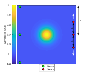
(a) Setup for plots of $\psi$.

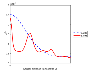
(b) Plots of $\psi$.

Figure 4:

These observations suggest the following algorithm in which we arrange frequencies into groups of increasing size and solve the bilevel problem for each group using the solution obtained for the previous group. We summarise this in Algorithm 2 which, for simplicity, is presented for one training model only; the notation ‘Bilevel Optimisation Algorithm($g_{k}$)’ means solving the bilevel optimisation problem (Algorithm 5.4.2) on the $k$th frequency group $g_{k}$.

Algorithm 2 Bilevel Frequency Continuation

1:Inputs: $\mathcal{P}_{0}$, $\boldsymbol{m}_{0}$, frequencies $\{\omega_{1}<\omega_{2}<...<\omega_{N{\omega}}\}\in\mathcal{W}$, $\boldsymbol{m}^{\prime}$

2:Group frequencies into $N_{f}$ groups $\{g_{1}$, $g_{2}$,$\ldots$, $g_{N_{f}}\}$

3:for $k=1$ to $N_{f}$ do

4:$[\mathcal{P}_{\min},\boldsymbol{m}^{FWI}]\leftarrow$ Bilevel Optimisation Algorithm($g_{k}$)

5:$\mathcal{P}_{0}\leftarrow\mathcal{P}_{\min}$

6:$\boldsymbol{m}_{0}\leftarrow\boldsymbol{m}^{FWI}$

7:end for

8:Output: $\mathcal{P}_{\min}$

We illustrate the performance of Algorithm 2 in Figure 5. Each row of Figure 5 shows a plot of the upper-level objective function $\psi$ for the problem setup in Figure 4(a), starting at a low frequency on row one, and increasing to progressively higher frequencies/frequency groups. In Subfigure (a) we represent a typical starting guess for the parameter to be optimised, $\Delta$, by an open red circle. Here $\psi$ has one minimum, and the optimisation method finds it straightforwardly – see the full red circle in Subfigure (b). We then progress through higher frequency groups, using the solution at the previous step as a starting guess for the next, allowing eventually convergence to the global minimum of the highest frequency group and avoiding the spurious local minima.

(a) 0.5 Hz (b) 0.5 Hz (c) 1 and 2 Hz group (d) 1 and 2 Hz group (e) 4 and 5 Hz group (f) 4 and 5 Hz group Figure 5: Plots of the upper-level objective function in an illustration of the bilevel frequency continuation approach. The symbol denotes a starting guess, and the symbol denotes a minimum.

Remark 4.1.

Algorithm 2 is written for the optimisation of sensor positions $\mathcal{P}$ only. The experiments in [8, §5.1] indicate that the objective function $\psi$ does not become more oscillatory with respect to $\alpha$ for higher frequencies, and so the bilevel frequency-continuation approach is not required for optimising $\alpha$. Thus we recommend the user to begin optimising $\alpha$ alongside $\mathcal{P}$ only in the final frequency group, starting with a reasonable initial guess for $\alpha$, to keep iteration numbers low. If one does not have a reasonable starting guess for $\alpha$, it may be beneficial to begin optimising $\alpha$ straight away in the first frequency group.

4.5 Preconditioning the Hessian

While the solutions of Hessian systems are not required in the quasi-Newton method for the lower-level problem, such solutions are required to compute the gradient of the upper level objective function (see (3.1)). We solve these systems using a preconditioned conjugate gradient iteration, without explicilty forming the Hessian. As explained in §6, “adjoint-state” type arguments can be applied to efficiently compute matrix-vector multiplications with $H$; see also [16, Section 3.2]. In this section we discuss preconditioning techniques for the system (3.1). Our proposed preconditioners are:

• Preconditioner 1:

  $$P_{1}^{-1},\quad\text{where}\quad P_{1}=H(\boldsymbol{m}^{FWI}(\mathcal{P}_{0},\alpha_{0},\boldsymbol{m}^{\prime}),\mathcal{P}_{0},\alpha_{0}),$$

  i.e., the full Hesssian at some chosen design parameters $\mathcal{P}_{0}$ and $\alpha_{0}$.

  During the bilevel algorithm the design parameters $\mathcal{P},\alpha$ (and hence $\boldsymbol{m}^{FWI}(\mathcal{P},\alpha,\boldsymbol{m}^{\prime})$) may move away from the initial choice $\mathcal{P}_{0},\alpha_{0}$ and $\boldsymbol{m}^{FWI}(\mathcal{P}_{0},\alpha_{0},\boldsymbol{m}^{\prime})$ and the preconditioner may need to be recomputed using updated $\mathcal{P},\alpha$ to ensure its effectiveness. Here we recompute the preconditioner at the beginning of each new frequency group. The cost of computing this preconditioner, is relatively high – costing $M$ Helmholtz solves, for each source, frequency, and training model.

• Preconditioner 2:

  $$P_{2}^{-1},\quad\text{where}\quad P_{2}=\Gamma(\alpha_{0},\mu).$$

  This is cheap to compute as no PDE solves are required. In addition, this preconditioner is independent of the sensor positions $\mathcal{P}$, training models $\boldsymbol{m}^{\prime}$, FWI reconstructions $\boldsymbol{m}^{FWI}$ and frequency. When optimising sensor positions alone, the preconditioner therefore only needs to be computed once at the beginning of the bilevel algorithm. Even when optimising $\alpha$, this preconditioner does not need to be recomputed since it turns out to remain effective even when $\alpha$ is no longer near its initial guess.

Although we write the preconditioners above as the inverses of certain matrices, these are not computed in practice, rather the Cholesky factorisation of the relevant matrix is computed and used to compute the action of the inverse. To test the preconditioners we consider the solution of (3.1) in the following situation. We take a training model and configuration of sources and sensors as shown in Figure 6 and compute $\boldsymbol{m}^{FWI}$, using synthetic data, avoiding an inverse crime by computing the data and solution using different grids.

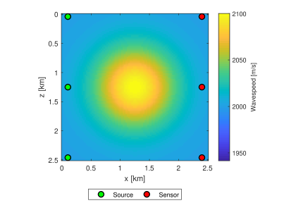
Figure 6: Ground truth model and acquisition setup used for preconditioining experiments.

We consider the CG/PCG method to have converged if $\|\textbf{r}_{n}\|_{2}/\|\textbf{r}_{0}\|_{2}\leq 10^{-6}$, where $\textbf{r}_{n}$ denotes the residual at the $n$th iteration and $\textbf{r}_{0}$ denotes the initial residual.

The aim of this experiment is to demonstrate the reduction in the number of iterations for PCG to converge, compared to the number of CG iterations (denoted $N_{i}$ here). We denote the number of iterations taken using Preconditioner 1 as $N_{i}^{P_{1}}$ and the number of iterations taken using Preconditioner 2 as $N_{i}^{P_{2}}$. As we have explained, the preconditioner $P_{1}$ depends on the sensor positions. Therefore we test two versions of $P_{1}$ – one where the sensor positions $\mathcal{P}_{0}$ are close to the current sensor positions $\mathcal{P}$ (i.e. close to those shown in Figure 6) and one where the sensor positions $\mathcal{P}_{0}$ are far from $\mathcal{P}$. We denote these preconditioners as $P_{1_{near}}$ and $P_{1_{far}}$ and their iterations counts as $N_{i}^{{P_{1}}_{near}}$ and $N_{i}^{{P_{1}}_{far}}$, respectively. We display these ‘near’ and ‘far’ sensor setups in Figure 7 (a) and (b), respectively.

(a) Sensor positions ‘near’ $\boldsymbol{p}$

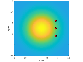
(b) Sensor positions ‘far’ from $\boldsymbol{p}$

Figure 7: Sensor positions used to compute the preconditioner $P_{1}$. This preconditioner is used to solve (3.1) for the problem shown in Figure 6.

We vary the regularisation parameter $\alpha$ and record the resulting number of CG/PCG iterations taken to solve (3.1). Table 1 shows the number of iterations needed to solve (3.1) when using the PCG method, as well as the percentage reduction in iterations (computed as the reduction in iterations divided by the original non-preconditioned number of iterations, expressed as a percentage and rounded to the nearest whole number). We see that preconditioner $P_{1}$ is very effective at reducing the number of iterations when the sensors $\mathcal{P}_{0}$ are close to $\mathcal{P}$. The number of iterations are reduced by between 85-96$\%$. When $\mathcal{P}_{0}$ is not close to $\mathcal{P}$ however, $P_{1}$ is not as effective. In this case, the PCG method is even worse than the CG method when $\alpha$ is small, but improves as $\alpha$ is increased, reaching approximately a 89$\%$ reduction in number of iterations at best. This motivates the update in this preconditioner as the sensors move far from their initial positions. The preconditioner $P_{2}$ produces a more consistent reduction in the number of iterations, ranging from 71-91$\%$.

$\alpha$	$N_{i}$	$N_{i}^{{P_{1}}_{near}}$	$\%$	$N_{i}^{{P_{1}}_{far}}$	$\%$	$N_{i}^{P_{2}}$	$\%$
0.5	153	21	86 $\%$	181	-18 $\%$	36	76 $\%$
1	132	17	87 $\%$	136	- 3 $\%$	35	73 $\%$
5	127	11	91 $\%$	62	51 $\%$	29	77 $\%$
10	137	9	93 $\%$	46	66 $\%$	26	81 $\%$
20	143	8	94 $\%$	32	78 $\%$	21	85 $\%$
50	158	7	96 $\%$	24	85 $\%$	17	89 $\%$
100	162	6	96 $\%$	16	90 $\%$	14	91 $\%$

Table 1: Effect of varying Tikhonov regularisation weight $\alpha$ on solving (3.1) using PCG, using two versions of the preconditioner $P_{1}$ and the preconditioner $P_{2}$. The convex parameter is constant at $\mu=10^{-8}$.

These iteration counts must then be considered in the context of the overall cost of solving the bilevel problem in [8, Section 5.2.2.1]. In this cost analysis we show that, in general, $P_{2}$ is a more cost effective preconditioner than $P_{1}$ when $M$ is large.

4.6 Parallelisation

Examination of Algorithm 1 reveals that its parallelisation over training models is straightforward. For each $\boldsymbol{m}^{\prime}\in\mathcal{M}^{\prime}$, the lower-level solutions $\boldsymbol{m}^{FWI}(\boldsymbol{p},\boldsymbol{m}^{\prime})$ can be computed independently. Then, from the loop beginning at Step 2 of Algorithm 1, the main work in computing the gradient of $\psi$ is also independent of $\boldsymbol{m}^{\prime}$, with only the finally assembly of the gradient (by (3.11) (3.3)) having to take place outside of this parallelisation. The algorithm was parallelised using the parfor function in Matlab. [8, Section 5.3] demonstrated, using strong and weak scaling, that the problem scaled well using up to $N_{m^{\prime}}$ processes.

5 Application to a Marmousi problem

In this section we apply our algorithm to find the optimal design parameters for the standard Marmousi benchmark, smoothed by applying a Gaussian filter horizontally and vertically (see Figure 8). We use the smoothed model here, combined with standard Tikhonov regularisation (as in (2.35)), because we want to assess the performance of our design parameter optimisation, rather than the choice of regularisation. The algorithm we propose could also be combined with other regularisation techniques more suitable for non-smooth problems.

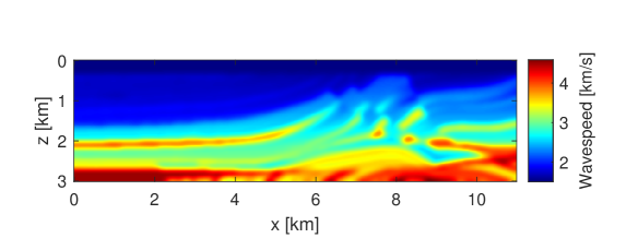
Figure 8: Smooth Marmousi model.

We discretised the model in Figure 8 using a $440\times 121$ rectangular grid, yielding a grid spacing of 25m in both the $x$ (horizontal) and $z$ (vertical) directions. We split this horizontally into five slices of equal size (Figure 9) (each with 10648 model parameters), and used Slices 1,2,4,5 as training models, reserving Slice 3 as a testing model for evaluation of the optimal parameters on a related but (different) model. This idea was motivated by experiments in [12, Section 4.3] and [11, Section 5.1].

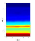
(a) Slice 1

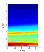
(b) Slice 2

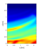
(c) Slice 3

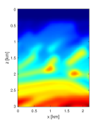
(d) Slice 4

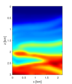
(e) Slice 5

Figure 9: Smooth Marmousi model divided into individual slices.

5.1 Training

We optimised the positions (i.e., both coordinates) of 20 sensors, as well as the regularisation weight $\alpha$. The initial set of non-optimised positions is illustrated in Figure 10(a), where we have chosen to superimpose this on Slice 2. In a transmission set-up, 10 sources are positioned uniformly along a line on the left-hand side, and 20 sensors are uniformly spaced along a line on the opposite side. The same starting setup is used for all four training models. Our non-optimised choice of regularisation weight is $\alpha=10$, which was experimentally observed to generate good quality reconstructions in general. The non-optimised parameters were used as the starting guesses for Algorithm 1.

The starting guess for computing the FWI reconstructions of each training model (lower level solutions) was taken to be $m=1/c^{2}$, where $c$ is a smoothly vertically varying wavespeed, increasing with depth, horizontally constant, and containing no information on any of the structures in the training models. (See Figure 10(b).)

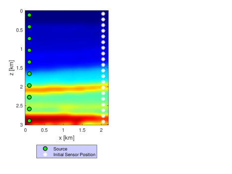
(a)

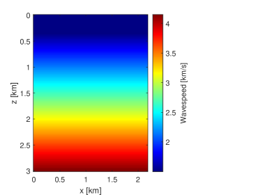
(b)

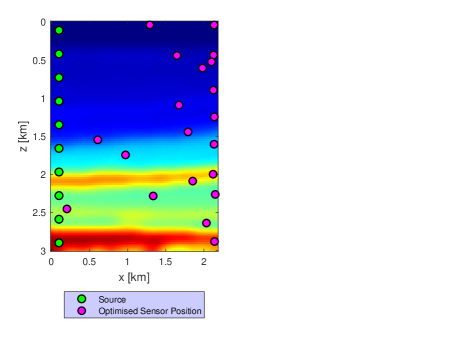
(c)

Figure 10: (a) Source positions and non-optimised sensor positions; (b) Initial guess for the wavespeed for each training model; (c) Source positions and optimised sensor positions after application of Algorithm 1 using four training models. Illustrations (a),(c) are presented on slice 2 for convenience.

We implemented Algorithm 1 with bilevel frequency continuation (Algorithm 2), using four frequency groups in the range 0.5 Hz to 6 Hz. In the first three groups, only the sensor positions were optimised, while in the final group the regularisation weight was optimised as well. The lower-level problem was solved to a tolerance of $\|\nabla\phi\|_{2}\leq 10^{-10}$, while the CG iteration for the Hessian system (3.1) (required for the upper-level gradient computation) was terminated when a Euclidean norm relative residual reduction of $10^{-15}$ was achieved. In the optimisation at the upper level, for each frequency group, iteration was terminated when any one of the following conditions was satisfied: (i) the infinity norm of the gradient (projected onto the feasible design space) was smaller than $10^{-10}$, (ii) the updates to $\psi$ or the optimisation parameters stalled or (iii) 100 iterations were reached. (Note that condition (i) is similar to the condition proposed in [4, Equation 6.1].)

Results: The optimised sensor positions are displayed in Figure 10(c) (again superimposed on Slice 2). We note that many sensors have remained on the right-hand side of the domain, close to their starting guesses, but they are no longer uniformly spaced along a straight line. In the upper half of the domain, the optimised sensors all lie in the top right quadrant, possibly because these are the best locations to measure both waves transmitted directly from the sources, as well as waves generated by upper sources and reflected from the layers below of higher wavespeed. In the lower half there are three sensors that have moved left into the interior. The overlay on slice 2 in Figure 10(c) shows that these are found near layers of different wavespeeds and potentially stimulated by these features. The optimal regularisation weight for this setup was found to be 6.855.

In Figures 11 and 12 we display the reconstructions of the training models at, respectively, the non-optimised and optimised design parameters with the ground truths displayed in Figure 8. (Note that the colour maps are scaled to be in the same range; i.e., the colours correspond to the same values in each slice.) We observe that the non-optimised design parameters yield reconstructions that, in general, identify the large-scale structures present in the ground truth. However, the shapes and wavespeed values in the structures are not always correct. For example, in Slices 1 and 2, the layer of higher wavespeed at depth approximately 2.1 km has wavespeed values that are too low, and the layer itself is not the correct thickness

The reconstruction of Slice 4 is relatively poor and many of the details present in the ground truth are missing, for example, the curving bump at around 2.25-2.5 km depth has been reconstructed with missing chunks, and the isolated area of high wavespeed at about 2 km in depth and 1.75 km across is missing. For Slice 5, the general structure is correct, but some of the wavespeed values are incorrect, particularly near the bottom of the domain.

With the optimised parameters (Figure 12), many of the issues observed in Figure 11 have been improved on. Both the geometry and wavespeed values in these reconstructions appear closer to the ground truth. The images have appeared to ‘sharpen’ up, particularly in the upper part of the domain, and the finer features of structures and boundaries between the layers have become evident. Some features that are missing in the starting guess now appear in the optimised reconstructions although there remain areas that could be improved.

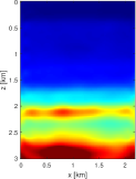
(a) Slice 1

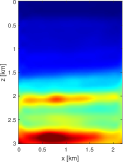
(b) Slice 2

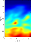
(c) Slice 4

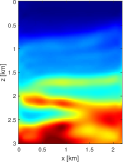
(d) Slice 5

Figure 11: FWI Reconstructions of training models using the non-optimised design parameters.

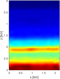
(a) Slice 1

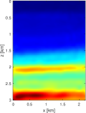
(b) Slice 2

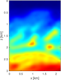
(c) Slice 4

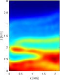
(d) Slice 5

Figure 12: FWI Reconstructions of training models using the optimised design parameters.

For more insight into the quality of the reconstructions in Figures 11 and 12, the relative percentage errors were computed (for each model parameter) using the formula

$$\text{Relative Percentage Error}=\left|\frac{\text{Reconstructed Value - True Value}}{\text{True Value}}\right|\times 100.$$ (5.1)

and these are plotted in Figures 13 and 14 respectively. Since darker shading represents larger error, with white indicating zero error, here we see more clearly the conspicuous benefit of optimisation of the design parameters.

In Table 2, we report the mean relative percentage error for the reconstructions using the optimised parameters. This shows that, on average, the errors that are low for all training models. Here we also report the Structural Similarity Index (SSIM) between the ground truths and the optimised reconstructions. SSIM is a quality metric commonly used in imaging [30, Section III B]. A good similarity between images is indicated by values of SSIM that are close to 1. The SSIM values were computed using the ssim function in Matlab’s Image Processing Toolbox.

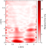
(a) Slice 1

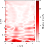
(b) Slice 2

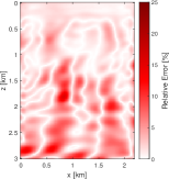
(c) Slice 4

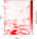
(d) Slice 5

Figure 13: Absolute value of the relative percentage error in the reconstructions using the non-optimised parameters.

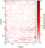
(a) Slice 1

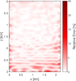
(b) Slice 2

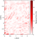
(c) Slice 4

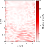
(d) Slice 5

Figure 14: Absolute value of the relative percentage error in the reconstructions at the optimised parameters.

Slice	Mean Relative Error ($\%$)	SSIM
1	0.937	0.962
2	1.159	0.943
4	1.017	0.957
5	1.055	0.948

Table 2: Measures of quality of the FWI reconstructions of training models at optimised parameters.

5.2 Testing

Here we evaluate the optimal parameters found in §5.1 by applying FWI to Slice 3 of Figure 9 and comparing the results with those obtained using non-optimised parameters. For this test we added $1\%$ Gaussian white noise to the synthetic data.

Results: The ground truth, and reconstructions at the non-optimised and optimised parameters are shown in Figure 15.

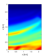
(a) Ground Truth

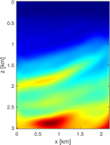
(b) Initial

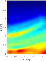
(c) Optimised

Figure 15: Ground truth testing model and its correspondng reconstructions at the non-optimised and optimised parameters.

While the reconstruction using the non-optimised parameters appears reasonable, the values of the wavespeed (particularly near the bottom of the domain) are quite inaccurate while the optimisation has yielded considerable improvement. The advantage of the optimisation is more obvious from the plots of the relative percentage error (5.1) given in Figure 16. Similarly to the training models, the improvement is most noticeable in the part of the domain below 2km. When using the optimised parameters, the mean relative error is $1.075$ and the SSIM is $0.949$: these values show that the reconstruction at the optimal parameters is indeed of good quality (and of similar quality to the reconstructed training models), and that there is a significant improvement over the non-optimised parameters.

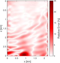
(a) Initial

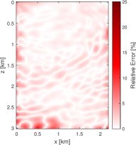
(b) Optimised

Figure 16: Absolute value of the relative percentage error in the FWI reconstructions of the testing model at the non-optimised and optimised parameters.

Conclusion:

The experiment shows that training on a set of ‘rough models’ has the potential to provide good design parameters for inverting data coming from some different unknown model, but with some similarity to the training set. Indeed, while the training and testing models above have differences, they also share some properties, such as the range of wavespeeds present and the fact that the wavespeed increases, on average, as the depth increases. Although outside the scope of the present paper, an important question now concerns the potential of the proposed method for geophysical problems, where (for example) rough surveys could be used to drive parameter optimisation for inversion from more extensive surveys.

Acknowledgements.  We thank Schlumberger Cambridge Research for financially supporting the PhD studentship of Shaunagh Downing within the SAMBa Centre for Doctoral Training at the University of Bath. The original concept for this research was proposed by Evren Yarman, James Rickett and Kemal Ozdemir (all Schlumberger) and we thank them all for many useful, insightful and supportive discussions. We also thank Matthias Ehrhardt (Bath), Romina Gaburro (Limerick), Tristan Van Leeuwen (Amsterdam), and Stéphane Operto and Hossein Aghamiry (Geoazur, Nice) for helpful comments and discussions.

We gratefully acknowledge support from the UK Engineering and Physical Sciences Research Council Grants EP/S003975/1 (SG, IGG, and EAS), EP/R005591/1 (EAS), and EP/T001593/1 (SG). This research made use of the Balena High Performance Computing (HPC) Service at the University of Bath.

6 Appendix – Computations with the gradient and Hessian of $\phi$

6.1 Gradient of $\phi$

Recall the formula for the gradient $\nabla\phi$ given in (2.43). Since we use a variant of the BFGS quasi-Newton algorithm to minimise $\phi$, the cost of this algorithm is dominated by the computation of $\phi$ and $\nabla\phi$. While efficient methods for computing these two quantities (using an ‘adjoint-state’ argument) are known, we state them again briefly here since (i) we do not know references where this procedure is written down at the PDE (non-discrete) level and (ii) the development motivates our approach for computing $\nabla\psi$ given in §3.1. A review of the adjoint-state method, and an alternative derivation of the gradient from a Lagrangian persepctive, are provided in [19], see also [16].

Theorem 6.1 (Formula for $\nabla\phi$).

For models $\boldsymbol{m},\boldsymbol{m}^{\prime}$, sensor positions $\mathcal{P}$, regularisation parameter $\alpha$ and each $k=1,\ldots,M$,

$$\frac{\partial\phi}{\partial m_{k}}(\boldsymbol{m},\mathcal{P},\alpha,\boldsymbol{m}^{\prime})\ =\ -\Re\sum_{s\in\mathcal{S}}\sum_{\omega\in\mathcal{W}}\bigg{(}\mathcal{G}_{\boldsymbol{m},\omega}(\beta_{k}u(\boldsymbol{m},\omega,s)),\lambda(\boldsymbol{m},\mathcal{P},\omega,s,\boldsymbol{m}^{\prime})\bigg{)}_{\Omega\times\partial\Omega}\noindent+\Gamma(\alpha,\mu)\boldsymbol{m},$$ (6.1)

where, for each $\omega\in\mathcal{W}$ and $s\in\mathcal{S}$, $\lambda$ is the adjoint solution:

$$\lambda(\boldsymbol{m},\mathcal{P},\omega,s,\boldsymbol{m}^{\prime})=\mathscr{S}_{\boldsymbol{m},\omega}^{*}\left(\begin{array}[]{l}\mathcal{R}(\mathcal{P})^{*}\boldsymbol{\varepsilon}(\boldsymbol{m},\mathcal{P},\omega,s,\boldsymbol{m}^{\prime})\\ 0\end{array}\right).$$ (6.4)

Proof.

Here we adopt the convention in Notation 3.2 and use (2.34) to write (2.43) as

$$\frac{\partial\phi}{\partial m_{k}}(\boldsymbol{m},\mathcal{P},\alpha)\ =\ -\Re\left\langle\mathcal{R}(\mathcal{P})\frac{\partial u}{\partial m_{k}}(\boldsymbol{m}),\boldsymbol{\varepsilon}(\boldsymbol{m},\mathcal{P})\right\rangle+\Gamma(\alpha,\mu)\boldsymbol{m}$$

$$=\ -\Re\left(\frac{\partial u}{\partial m_{k}}(\boldsymbol{m}),\mathcal{R}(\mathcal{P})^{*}\boldsymbol{\varepsilon}(\boldsymbol{m},\mathcal{P})\right)_{\Omega}+\Gamma(\alpha,\mu)\boldsymbol{m}.$$ (6.5)

Using (2.48), the first term on the right-hand side of (6.5) becomes

$$-\Re\bigg{(}(1,0)\,\mathscr{S}_{\boldsymbol{m},\omega}\mathcal{G}_{\boldsymbol{m},\omega}(\beta_{k}u(\boldsymbol{m})),\,\mathcal{R}(\mathcal{P})^{*}\boldsymbol{\varepsilon}(\boldsymbol{m},\mathcal{P})\bigg{)}_{\Omega}$$

$$\quad\quad=\ -\Re\left(\mathscr{S}_{\boldsymbol{m},\omega}\mathcal{G}_{\boldsymbol{m},\omega}(\beta_{k}u(\boldsymbol{m})),\,\left(\begin{array}[]{l}\mathcal{R}(\mathcal{P})^{*}\boldsymbol{\varepsilon}(\boldsymbol{m},\mathcal{P})\\ 0\end{array}\right)\right)_{\Omega\times\partial\Omega}$$ (6.8)

$$\quad\quad=\ -\Re\left(\mathcal{G}_{\boldsymbol{m},\omega}(\beta_{k}u(\boldsymbol{m})),\,\lambda(\boldsymbol{m},\mathcal{P})\right)_{\Omega\times\partial\Omega},$$ (6.9)

where we used (2.26). Combining (6.5) and (6.9) yields the result. ∎

Thus, given $\boldsymbol{m},\mathcal{P},\alpha,\boldsymbol{m}^{\prime}$ and assuming $u(\boldsymbol{m}^{\prime},s,\omega)$ is known for all $s,\omega$, to find $\nabla\phi$, we need only two Helmholtz solves for each $s$ and $\omega$, namely a solve to obtain $u(\boldsymbol{m},\omega,s)$ and an adjoint solve to obtain $\lambda(\boldsymbol{m},\mathcal{P},\omega,s,\boldsymbol{m}^{\prime})$. Algorithm 3 presents the steps involved.

Algorithm 3 Algorithm for Computing $\phi,\ \nabla\phi$

1:Inputs: $\mathcal{P}$, $\mathcal{W}$, $\mathcal{S}$, $\boldsymbol{m},\boldsymbol{m}^{\prime}$, $\alpha,\mu$ and $\textbf{u}(\boldsymbol{m}^{\prime},s,\omega)=(1,0)\mathscr{S}_{\boldsymbol{m}^{\prime},\omega}(\delta_{s})$

2:for $\omega\in\mathcal{W}$, $s\in\mathcal{S}$ do

3:Compute the primal wavefield $\textbf{u}(\boldsymbol{m},s,\omega)=(1,0)\mathscr{S}_{\boldsymbol{m},\omega}(\delta_{s})$

4:Compute $\boldsymbol{\varepsilon}(\boldsymbol{m},\mathcal{P},\omega,s,\boldsymbol{m}^{\prime})$ by (2.38)

5:Compute the adjoint wavefield $\boldsymbol{\lambda}(\boldsymbol{m},\mathcal{P},\omega,s,\boldsymbol{m}^{\prime})$ from (6.4)

6:end for

7:Compute $\phi$ from (2.37), (2.38).

8:Compute $\nabla\phi$ from (6.1)

Computing the gradient.  Using the discretisation scheme in §4.1 and restricting to the computation of a single term in the sum on the right-hand side, the numerical analogue of (6.1) is as follows.

The vector $\boldsymbol{\lambda}\in\mathbb{C}^{M}$ representing $\lambda(\boldsymbol{m},\mathcal{P},\omega,s,\boldsymbol{m}^{\prime})$ is computed by solving

$$A(\boldsymbol{m},\omega)^{*}\boldsymbol{\lambda}=\sum_{\boldsymbol{p}\in\mathcal{P}}\varepsilon_{\boldsymbol{p}}\mathbf{e}_{\boldsymbol{p}}\ ,\quad\text{where}\quad\varepsilon_{\boldsymbol{p}}=(R(\mathcal{P})\left(\mathbf{u}(\boldsymbol{m}^{\prime},\omega,s)-\mathbf{u}(\boldsymbol{m},\omega,s)\right))_{\boldsymbol{p}},$$

and $R(\mathcal{P})$ denotes the sliding cubic approximation (as described in §4.3) and $\mathbf{e}_{\boldsymbol{p}}$ represents the numerical realisation of the delta function situated at $\boldsymbol{p}$. Then the inner product in (6.1) is approximated by

$$-\Re\left(\omega^{2}d_{k}u_{k}\overline{\lambda_{k}}\right), \text{if}\quad k\quad\text{is an interior node},$$

$$-\Re\left((\omega^{2}d_{k}u_{k}+b_{k}\frac{{\rm i}\omega}{2\sqrt{m_{k}}}u_{k})\overline{\lambda_{k}}\right), \text{if}\quad k\quad\text{is a boundary node}.$$

6.2 Matrix-vector multiplication with the Hessian

Differentiating (2.43) with respect to $m_{j}$, we obtain the Hessian $H$ of $\phi$,

$$H(\boldsymbol{m},\mathcal{P},\alpha,\boldsymbol{m}^{\prime})=H^{(1)}(\boldsymbol{m},\mathcal{P})+H^{(2)}(\boldsymbol{m},\mathcal{P},\boldsymbol{m}^{\prime})+\Gamma(\alpha,\mu),$$

with $H^{(1)}$ and $H^{(2)}$ defined by

$$\left(H^{(1)}(\boldsymbol{m},\mathcal{P})\right)_{j,k} \ =\ \Re\sum_{s\in\mathcal{S}}\sum_{\omega\in\mathcal{W}}\left\langle\mathcal{R}(\mathcal{P})\frac{\partial u}{\partial m_{j}}(\boldsymbol{m},\omega,s)\,,\,\mathcal{R}(\mathcal{P})\frac{\partial u}{\partial m_{k}}(\boldsymbol{m},\omega,s)\right\rangle,$$ (6.10)

$$\left(H^{(2)}(\boldsymbol{m},\mathcal{P},\boldsymbol{m}^{\prime})\right)_{j,k} \ =\ -\Re\sum_{s\in\mathcal{S}}\sum_{\omega\in\mathcal{W}}\left\langle\mathcal{R}(\mathcal{P})\frac{\partial^{2}u}{\partial m_{k}\partial m_{j}}(\boldsymbol{m},\omega,s)\,,\,\boldsymbol{\varepsilon}(\boldsymbol{m},\mathcal{P},\omega,s,\boldsymbol{m}^{\prime})\right\rangle.$$ (6.11)

Observe that $H^{(1)}$ is symmetric positive semidefinite, while $H^{(2)}$ is symmetric but possibly indefinite.

In the following two lemmas we obtain efficient formulae for computing $H^{(1)}\widetilde{\boldsymbol{m}}$ and $H^{(2)}\widetilde{\boldsymbol{m}}$ for any $\widetilde{\boldsymbol{m}}\in\mathbb{R}^{M}$. These make use of ‘adjoint state’ arguments. Analogous formulae in the discrete case are given in [16]. Before we begin, for any $\widetilde{\boldsymbol{m}}=(\widetilde{m}_{1},\dots,\widetilde{m}_{M})\in\mathbb{R}^{M}$, we define

$$\widetilde{m}=\sum_{k}\widetilde{m}_{k}\beta_{k}.$$ (6.12)

Lemma 6.2 (Adjoint-state formula for multiplication by $H^{(1)}(\boldsymbol{m},\mathcal{P})$).

For any $\boldsymbol{m},\boldsymbol{m}^{\prime}\in\mathbb{R}^{M}$, $\omega\in\mathcal{W}$ and $s\in\mathcal{S}$, let $u(\boldsymbol{m},\omega,s)$ be the wavefield defined by (2.31), and set

$$v(\boldsymbol{m},\omega,s,\widetilde{\boldsymbol{m}})=(1,0)\,\mathscr{S}_{\boldsymbol{m},\omega}\,\mathcal{G}_{\boldsymbol{m},\omega}\left(\begin{array}[]{l}\widetilde{m}u(\boldsymbol{m},\omega,s)\\ \widetilde{m}u(\boldsymbol{m},\omega,s)|_{\partial\Omega}\end{array}\right).$$ (6.15)

Then, for each $j=1,\ldots,M$,

$$(H^{(1)}(\boldsymbol{m},\mathcal{P},\boldsymbol{m}^{\prime})\widetilde{\boldsymbol{m}})_{j} \quad=\Re\sum_{s\in\mathcal{S}}\sum_{\omega\in\mathcal{W}}\left(\mathcal{G}_{\boldsymbol{m},\omega}\left(\begin{array}[]{l}\beta_{j}u(\boldsymbol{m},\omega,s)\\ \beta_{j}u(\boldsymbol{m},\omega,s)|_{\partial\Omega}\end{array}\right),\mathscr{S}_{\boldsymbol{m},\omega}^{*}\left(\begin{array}[]{l}{\mathcal{R}}(\mathcal{P})^{*}{\mathcal{R}}(\mathcal{P})v(\boldsymbol{m},\omega,s,\widetilde{\boldsymbol{m}})\\ 0\end{array}\right)\right)_{\Omega\times\partial\Omega}.$$ (6.20)

Proof.

Using the convention in Notation 3.2, the definition of $\widetilde{m}$, the linearity of $\mathscr{S}_{\boldsymbol{m},\omega}$ and $\mathcal{G}_{\boldsymbol{m},\omega}$ and then (2.48), we can write

$$v(\boldsymbol{m},\widetilde{\boldsymbol{m}})=(1,0)\,\sum_{k}\,\mathscr{S}_{\boldsymbol{m},\omega}\,\mathcal{G}_{\boldsymbol{m},\omega}\left(\begin{array}[]{l}\beta_{k}u(\boldsymbol{m})\\ \beta_{k}u(\boldsymbol{m})|_{\partial\Omega}\end{array}\right)\,\widetilde{m}_{k}=\sum_{k}\frac{\partial u}{\partial m_{k}}(\boldsymbol{m})\,\widetilde{m}_{k}.$$ (6.23)

Then, using (6.10), (6.23), and then (2.34), we obtain

$$(H^{(1)}(\boldsymbol{m},\mathcal{P},\boldsymbol{m}^{\prime})\widetilde{\boldsymbol{m}})_{j} =\Re\sum_{k}\left\langle\mathcal{R}(\mathcal{P})\frac{\partial u}{\partial m_{j}}(\boldsymbol{m})\,,\,\mathcal{R}(\mathcal{P})\frac{\partial u}{\partial m_{k}}(\boldsymbol{m})\right\rangle\widetilde{m}_{k}$$

$$=\Re\left\langle\mathcal{R}(\mathcal{P})\frac{\partial u}{\partial m_{j}}(\boldsymbol{m})\,,\,\mathcal{R}(\mathcal{P})v(\boldsymbol{m},\boldsymbol{m}^{\prime})\right\rangle=\Re\left(\frac{\partial u}{\partial m_{j}}(\boldsymbol{m})\,,\,\mathcal{R}(\mathcal{P})^{*}\mathcal{R}(\mathcal{P})v(\boldsymbol{m},\boldsymbol{m}^{\prime})\right)_{\Omega}.$$

Then substituting for $\partial u/\partial m_{j}$ using (2.48), and proceeding analogously to (6.9), we have

$$(H^{(1)}(\boldsymbol{m},\mathcal{P},\boldsymbol{m}^{\prime})\widetilde{\boldsymbol{m}})_{j} =\Re\left(\mathcal{G}_{\boldsymbol{m},\omega}\left(\begin{array}[]{l}\beta_{j}u(\boldsymbol{m})\\ \beta_{j}u(\boldsymbol{m})|_{\partial\Omega}\end{array}\right)\,,\,\mathscr{S}_{m,\omega}^{*}\left(\begin{array}[]{l}\mathcal{R}(\mathcal{P})^{*}\mathcal{R}(\mathcal{P})v(\boldsymbol{m},\boldsymbol{m}^{\prime})\\ 0\end{array}\right)\right)_{\Omega\times\partial\Omega}.$$

Recalling Notation 3.2, this completes the proof. ∎

This lemma shows that (for each $\omega,s$) computing $H^{(1)}\widetilde{\boldsymbol{m}}$ requires only three Helmholtz solves, namely those required to compute $u$, $v$ and, in addition, the second argument in the inner products (6.20). Computing $H^{(2)}\widetilde{\boldsymbol{m}}$ is a bit more complicated. For this we need the following formula for the second derivatives of $u$ with respect to the model.

$$\left(\begin{array}[]{l}\frac{\partial^{2}u}{\partial m_{j}\partial m_{k}}\\ \frac{\partial^{2}u}{\partial m_{j}\partial m_{k}}|_{\partial\Omega}\end{array}\right) =\mathscr{S}_{\boldsymbol{m},\omega}\,\left[\mathcal{G}_{\boldsymbol{m},\omega}\left(\begin{array}[]{l}u_{j,k}\\ u_{j,k}|_{\partial\Omega}\end{array}\right)-\left(\begin{array}[]{l}0\\ \left(\frac{{\rm i}\omega}{4m^{3/2}}\right)\beta_{j}\beta_{k}u|_{\partial\Omega}\end{array}\right)\right],$$ (6.30)

where

$$u_{j,k}(\boldsymbol{m},\omega,s)=\beta_{j}\frac{\partial u}{\partial m_{k}}(\boldsymbol{m},\omega,s)+\beta_{k}\frac{\partial u}{\partial m_{j}}(\boldsymbol{m},\omega,s).\$$ (6.31)

The formulae (6.30), (6.31) are obtained by writing out (2.48) explicitly and differentiating with respect to $m_{j}$. Analogous second derivative terms appear in, e.g., [20] and [15]. However these are presented in the context of a forward problem consisting of solution of a linear algebraic system and so the detail of the PDEs being solved at each step is less explicit than here.

Lemma 6.3 (Adjoint-state formula for $H^{(2)}(\boldsymbol{m},\mathcal{P},\boldsymbol{m}^{\prime})\,\widetilde{\boldsymbol{m}}$).

For each $j=1,\ldots,M$,

$$\left(H^{(2)}(\boldsymbol{m},\mathcal{P},\boldsymbol{m}^{\prime})\widetilde{\boldsymbol{m}}\right)_{j} =-\Re\sum_{s\in\mathcal{S}}\sum_{\omega\in\mathcal{W}}\left[\left(\mathcal{G}_{\boldsymbol{m},\omega}\left(\begin{array}[]{l}\beta_{j}v(\boldsymbol{m},\omega,s,\boldsymbol{m}^{\prime})\\ \beta_{j}v(\boldsymbol{m},\omega,s,\boldsymbol{m}^{\prime})|_{\partial\Omega}\end{array}\right),\lambda(\boldsymbol{m},\mathcal{P},\omega,s,\boldsymbol{m}^{\prime})\right)_{\Omega\times\partial\Omega}\right.$$ (6.34)

$$\quad\quad\quad\quad+\left.\left(\mathcal{G}_{\boldsymbol{m},\omega}\left(\begin{array}[]{l}\beta_{j}u(\boldsymbol{m},\omega,s)\\ \beta_{j}u(\boldsymbol{m},\omega,s)|_{\partial\Omega}\end{array}\right),\mathscr{S}_{\boldsymbol{m},\omega}^{*}\left(\widetilde{m}\mathcal{G}_{\boldsymbol{m},\omega}\lambda(\boldsymbol{m},\mathcal{P},\omega,s,\boldsymbol{m}^{\prime})\right)\right)_{\Omega\times\partial\Omega}\right.$$ (6.37)

$$\quad\quad\quad\quad\left.-\left(\frac{{\rm i}\omega}{4m^{3/2}}\beta_{j}\widetilde{m}u(\boldsymbol{m},\omega,s)\,,\,\lambda(\boldsymbol{m},\mathcal{P},\omega,s,\boldsymbol{m}^{\prime})\right)_{\partial\Omega}\right],$$ (6.38)

where $\lambda$ is defined in (6.4) and $v$ is defined in (6.15).

Proof.

Using Notation 3.2 and (2.34), we can write $(H^{(2)}(\boldsymbol{m},\mathcal{P}))_{j,k}$ in (6.11) as

$$\left(H^{(2)}(\boldsymbol{m},\mathcal{P})\right)_{j,k}=-\Re\left\langle\mathcal{R}(\mathcal{P})\frac{\partial^{2}u}{\partial m_{k}\partial m_{j}}(\boldsymbol{m}),\boldsymbol{\varepsilon}(\boldsymbol{m},\mathcal{P})\right\rangle =-\Re\left(\frac{\partial^{2}u}{\partial m_{k}\partial m_{j}}(\boldsymbol{m}),\mathcal{R}(\boldsymbol{p})^{*}\boldsymbol{\varepsilon}(\boldsymbol{m},\mathcal{P})\right)_{\Omega}.$$ (6.39)

Then, substituting (6.30) into (6.39) and recalling (6.4), we obtain

$$(H^{(2)}(\boldsymbol{m},\mathcal{P}))_{j,k} =-\Re\left(\mathcal{G}_{\boldsymbol{m},\omega}\left(\begin{array}[]{l}u_{j,k}\\ u_{j,k}|_{\partial\Omega}\end{array}\right)-\left(\begin{array}[]{l}0\\ \left(\frac{{\rm i}\omega}{4m^{3/2}}\right)\beta_{j}\beta_{k}u\end{array}\right)\,,\,\lambda(\boldsymbol{m},\mathcal{P})\right)_{\Omega\times\partial\Omega}.$$ (6.44)

Before proceeding with (6.44) we first note that, by (6.31), (6.12), and then (6.23), we have

$$\sum_{k}u_{j,k}\widetilde{m}_{k}=\beta_{j}\sum_{k}\frac{\partial u}{\partial m_{k}}(\boldsymbol{m})\widetilde{m}_{k}+\widetilde{m}\frac{\partial u}{\partial m_{j}}(\boldsymbol{m})=\ \beta_{j}v(\boldsymbol{m},\boldsymbol{m}^{\prime})+\widetilde{m}\frac{\partial u}{\partial m_{j}}(\boldsymbol{m}).$$ (6.45)

Then, by (6.44), (6.45) and linearity of $\mathcal{G}_{\boldsymbol{m},\omega}$,

$$(H^{(2)}(\boldsymbol{m},\mathcal{P})\widetilde{\boldsymbol{m}})_{j}\ =\ -\Re\left(\mathcal{G}_{\boldsymbol{m},\omega}\left(\begin{array}[]{l}\beta_{j}v(\boldsymbol{m},\boldsymbol{m}^{\prime})\\ \beta_{j}v(\boldsymbol{m},\boldsymbol{m}^{\prime})|_{\partial\Omega}\end{array}\right),\lambda(\boldsymbol{m},\mathcal{P})\right)_{\Omega\times\partial\Omega}$$ (6.48)

$$\quad-\Re\left(\mathcal{G}_{\boldsymbol{m},\omega}\left(\begin{array}[]{l}\widetilde{m}\frac{\partial u}{\partial m_{j}}(\boldsymbol{m})\\ \widetilde{m}\frac{\partial u}{\partial m_{j}}(\boldsymbol{m})|_{\partial\Omega}\end{array}\right)\,,\,\lambda(\boldsymbol{m},\mathcal{P})\right)_{\Omega\times\partial\Omega}$$ (6.51)

$$\quad+\Re\left(\left(\begin{array}[]{l}0\\ \frac{{\rm i}\omega}{4m^{3/2}}\beta_{j}\widetilde{m}u|_{\partial\Omega}\end{array}\right)\,,\,\lambda(\boldsymbol{m},\mathcal{P})\right)_{\Omega\times\partial\Omega}.$$ (6.54)

The first and third terms in (6.54) correspond to the first and third terms in (6.38). The second term in (6.54) can be written

$$-\Re\left(\left(\begin{array}[]{l}\frac{\partial u}{\partial m_{j}}(\boldsymbol{m})\\ \frac{\partial u}{\partial m_{j}}(\boldsymbol{m})|_{\partial\Omega}\end{array}\right)\,,\,\widetilde{m}\mathcal{G}_{\boldsymbol{m},\omega}^{*}\lambda(\boldsymbol{m},\mathcal{P})\right)_{\Omega\times\partial\Omega}=-\Re\left(\mathscr{S}_{\boldsymbol{m},\omega}\mathcal{G}_{\boldsymbol{m},\omega}\left(\begin{array}[]{l}\beta_{k}u(\boldsymbol{m})\\ \beta_{k}u(\boldsymbol{m})|_{\partial\Omega}\end{array}\right)\,,\,\widetilde{m}\mathcal{G}_{\boldsymbol{m},\omega}^{*}\lambda(\boldsymbol{m},\mathcal{P})\right)_{\Omega\times\partial\Omega}$$

(where we also used (2.48)), and this corresponds to the second term in (6.38), completing the proof. ∎

As noted in [16, Section 3.3], the solution of a Hessian system with a matrix-free conjugate gradient algorithm requires the solution to $2+2N_{i}$ PDEs, where $N_{i}$ is the number of conjugate gradient iterations performed.

Discussion 6.4 (Cost of matrix-vector multiplication with $H$).

Lemmas 6.2 and 6.3 show that, to compute the product $H(\boldsymbol{m},\mathcal{P},\boldsymbol{m}^{\prime})\widetilde{\boldsymbol{m}}$ for any $\widetilde{\boldsymbol{m}}\in\mathbb{R}^{M}$ the Helmholtz solves required are (i) computation of $u$ in (2.31), (ii) computation of $\lambda$ in (6.4), (iii) computation of $v$ in (6.15), and finally (iv) the more-complicated adjoint solve

$$z:=\mathscr{S}_{\boldsymbol{m},\omega}^{*}\left[\left(\begin{array}[]{l}{\mathcal{R}}(\mathcal{P})^{*}{\mathcal{R}}(\mathcal{P})v(\boldsymbol{m},\omega,s,\widetilde{\boldsymbol{m}})\\ 0\end{array}\right)-\widetilde{m}\mathcal{G}_{\boldsymbol{m},\omega}\lambda(\boldsymbol{m},\mathcal{P},\omega,s,\boldsymbol{m}^{\prime})\right]$$

The remainder of the calculations in (6.20) and (6.38) require only inner products and no Helmholtz solves.

References

- [1] H. Aghamiry, A. Gholami, and S. Operto, Full waveform inversion by proximal newton method using adaptive regularization, Geophysical Journal International, 224 (2021), pp. 169–180.
- [2] A. Asnaashari, R. Brossier, S. Garambois, F. Audebert, P. Thore, and J. Virieux, Regularized seismic full waveform inversion with prior model information, Geophysics, 78 (2013), pp. R25–R36.
- [3] B. Brown, T. Carr, and D. Vikara, Monitoring, verification, and accounting of co2 stored in deep geologic formations, US Department of Energy National Energy Technology Laboratory, (2009).
- [4] R. H. Byrd, P. Lu, J. Nocedal, and C. Zhu, A limited memory algorithm for bound constrained optimization, SIAM Journal on Scientific Computing, 16 (1995), pp. 1190–1208.
- [5] C. Crockett and J. A. Fessler, Bilevel methods for image reconstruction, arXiv preprint arXiv:2109.09610, (2021).
- [6] S. Dempe, Bilevel Optimization: Theory, Algorithms and Applications, vol. Preprint 2018-11, TU Bergakademie Freiberg, Fakultät für Mathematik und Informatik, 2018.
- [7] S. Dempe and A. Zemkoho, eds., Bilevel Optimization: Advances and Next Challenges, vol. 161, Springer series on Optimization and its Applications, 2020.
- [8] S. Downing, Optimising Seismic Imaging via Bilevel Learning: Theory and Algorithms, PhD thesis, University of Bath, 2022. https://researchportal.bath.ac.uk/en/studentTheses/optimising-seismic-imaging-via-bilevel-learning-theory-and-algori.
- [9] B. Granzow, L-BFGS-B: A pure MATLAB implementation of L-BFGS-B. https://github.com/bgranzow/L-BFGS-B.
- [10] L. Guasch, O. C. Agudo, M. X. Tang, P. Nachev, and M. Warner, Full-waveform inversion imaging of the human brain, NPJ Digital Medicine, 3 (2020), pp. 1–12.
- [11] E. Haber, L. Horesh, and L. Tenorio, Numerical methods for experimental design of large-scale linear ill-posed inverse problems, Inverse Problems, 24 (2008), p. 055012.
- [12] E. Haber and L. Tenorio, Learning regularization functionals—a supervised training approach, Inverse Problems, 19 (2003), p. 611.
- [13] Q. He and Y. Wang, Inexact newton-type methods based on lanczos orthonormal method and application for full waveform inversion, Inverse problems, 36 (2020), pp. 115007–27.
- [14] F. Lucka, M. Pérez-Liva, B. E. Treeby, and B. T. Cox, High resolution 3D ultrasonic breast imaging by time-domain full waveform inversion, Inverse Problems, 38 (2021), p. 025008.
- [15] L. Métivier, R. Brossier, S. Operto, and J. Virieux, Second-order adjoint state methods for full waveform inversion, in EAGE 2012-74th European Association of Geoscientists and Engineers Conference and Exhibition, 2012.
- [16] , Full waveform inversion and the truncated newton method, SIAM Review, 59 (2017), pp. 153–195.
- [17] L. Métivier, P. Lailly, F. Delprat-Jannaud, and L. Halpern, A 2d nonlinear inversion of well-seismic data, Inverse problems, 27 (2011), p. 055005.
- [18] P. A. Narbel, J. P. Hansen, and J. R. Lien, Energy Technologies and Economics, Springer, 2014.
- [19] R. E. Plessix, A review of the adjoint-state method for computing the gradient of a functional with geophysical applications, Geophysical Journal International, 167 (2006), pp. 495–503.
- [20] R. G. Pratt, C. Shin, and G. J. Hick, Gauss–Newton and full Newton methods in frequency–space seismic waveform inversion, Geophysical Journal International, 133 (1998), pp. 341–362.
- [21] R. E. Sheriff and L. P. Geldart, Exploration Seismology, Cambridge University Press, 1995.
- [22] F. Sherry, M. Benning, J. C. De los Reyes, M. J. Graves, G. Maierhofer, G. Williams, C. B. Schönlieb, and M. J. Ehrhardt, Learning the sampling pattern for MRI, IEEE Transactions on Medical Imaging, 39 (2020), pp. 4310–4321.
- [23] A. Sinha, P. Malo, and K. Deb, A review on bilevel optimization: From classical to evolutionary approaches and applications, IEEE Transactions on Evolutionary Computation, 22 (2018), pp. 276–295.
- [24] L. Sirgue and R. G. Pratt, Efficient waveform inversion and imaging: A strategy for selecting temporal frequencies, Geophysics, 69 (2004), pp. 231–248.
- [25] A. Tarantola, Inverse Problem Theory and Methods for Model Parameter Estimation, SIAM, 2005.
- [26] T. van Leeuwan, Simple FWI. https://github.com/TristanvanLeeuwen/SimpleFWI, 2014.
- [27] T. van Leeuwen and F. J. Herrmann, A penalty method for pde-constrained optimization in inverse problems, Inverse Problems, 32 (2016), p. 015007.
- [28] T. van Leeuwen and W. A. Mulder, A comparison of seismic velocity inversion methods for layered acoustics, Inverse Problems, 26 (2009), p. 015008.
- [29] J. Virieux and S. Operto, An overview of full-waveform inversion in exploration geophysics, Geophys., 74 (2009), pp. WCC127–WCC152.
- [30] Z. Wang, A. C. Bovik, H. R. Sheikh, and E. P. Simoncelli, Image quality assessment: from error visibility to structural similarity, IEEE Transactions on Image Processing, 13 (2004), pp. 600–612.
- [31] S. Wright, J. Nocedal, et al., Numerical Optimization, Springer Science, 35 (1999), p. 7.