Automatic Locally Robust Estimation with Generated Regressors

Abstract

Many economic and causal parameters of interest depend on generated regressors. Examples include structural parameters in models with endogenous variables estimated by control functions and in models with sample selection, treatment effect estimation with propensity score matching, and marginal treatment effects. Inference with generated regressors is complicated by the very complex expression for influence functions and asymptotic variances. To address this problem, we propose Automatic Locally Robust/debiased GMM estimators in a general setting with generated regressors. Importantly, we allow for the generated regressors to be generated from machine learners, such as Random Forest, Neural Nets, Boosting, and many others. We use our results to construct novel Doubly Robust and Locally Robust estimators for the Counterfactual Average Structural Function and Average Partial Effects in models with endogeneity and sample selection, respectively. We provide sufficient conditions for the asymptotic normality of our debiased GMM estimators and investigate their finite sample performance through Monte Carlo simulations.

Keywords: Local robustness, orthogonal moments, double robustness, semiparametric estimation, bias, GMM. JEL Classification: C13; C14; C21; D24

1 Introduction

Many economic and causal parameters of interest depend on generated regressors. Leading examples include the Counterfactual Average Structural Function (CASF) in models with endogenous variables estimated by control functions (see, e.g., Stock,, 1989, 1991; Blundell and Powell,, 2004), Average Partial Effects (APE) in sample selection models (see, e.g., Das et al.,, 2003), Propensity Score Matching (PSM) (see, e.g., Heckman et al.,, 1998), and Marginal Treatment Effects (MTE) using Local Instrumental Variables (see, e.g., Heckman and Vytlacil,, 2005). There are currently no general econometric methods for inference on these parameters allowing for generated regressors obtained by machine learning. The goal of this paper is to propose Automatic Locally Robust/Debiased estimators of and inference on structural parameters in such models. The estimators and inferences that we propose are automatic in the sense that influence functions and asymptotic variances are estimated automatically from data and identifying moments. There is no need to find their analytic shape.

We extend Chernozhukov et al., 2022a ’s results to build debiased moment conditions in the presence of nonparametric/semiparametric generated regressors. By applying the chain rule, the debiasing correction term can be decomposed into one accounting for the first step, which is used to generate a regressor, and the term accounting for the second step, where the outcome variable is regressed onto the generated variable (among other covariates). Chernozhukov et al., 2022a construct debiased moment conditions which account for this second step (with no generated regressor). Our paper provides the additional correction term that accounts for (i) the plug-in of generated regressors in the moment condition and (ii) the effect of generated regressor on the estimation of the second step.

Each of the two correction terms depends on additional nuisance parameters. Under a linearization assumption (as in, e.g., Newey,, 1994; Ichimura and Newey,, 2022), we show how the additional nuisance parameters in the correction term can be estimated separately without knowing their specific analytic shape. This process is called automatic estimation (see Chernozhukov et al., 2022b, ). Automatic estimation is particularly well motivated in the case of generated regressors, where the nuisance parameters in the correction term take complex shapes (see, for instance, Hahn and Ridder,, 2013; Mammen et al.,, 2016; Escanciano et al.,, 2014).

As a leading application of our methods, we propose novel Automatic Locally Robust estimators for the CASF parameter of Blundell and Powell, (2004). This parameter is a linear functional of a second step function satisfying orthogonality conditions involving generated regressors (the control function) from a first step. We show that it is relatively straightforward to construct Automatic Doubly Robust estimators that are robust to functional form assumptions for the second step. For instance, a practical approach could be to fit a partially linear specification for the second step, like in Robinson, (1988), but with a non-parametric function of the generated regressors. Our results cover this case, in which the second step is semiparametric.

The Doubly Robust estimators are, however, not Locally Robust to the generated regressors in general. To construct fully Locally Robust estimators we use numerical derivatives to account for the presence of generated regressors. Fortunately, our automatic approach is amenable to any machine learning method for which out of sample predictions are available. Another approach could be to specify a model for the second step for which analytical derivatives are available, e.g., a partially linear model. We note that the Doubly Robust moment conditions are robust to this model being misspecified when the adjustment term is consistently estimated (see Remark 2.2).

We provide mild sufficient conditions for the asymptotic normality of the debiased GMM estimator. We illustrate the results with the CASF example. The finite sample performance of the proposed debiased estimator for the CASF is evaluated through Monte Carlo simulations. We use Lasso with different dictionaries (linear, quadratic, and one including interactions) to fit the first and second step parameters, as well as the nuisance parameters in the first and second step correction terms. Our Monte Carlo results confirm that the plug-in estimator is substantially biased. Correcting the moment condition for the second step estimation reduces de bias, but a first step correction must be also added to remove it totally throughout all the different specifications considered.

The paper builds on two different literatures. The first literature is the classical literature on semiparametric estimators with generated regressors, see Ichimura and Lee, (1991); Ahn and Powell, (1993); Heckman et al., (1998); Newey et al., (1999); Rothe, (2009); Imbens and Newey, (2009), among many others. The asymptotic properties of several estimators within this class is given, for example, by Escanciano et al., (2014), Hahn and Ridder, (2013, 2019) and Mammen et al., (2012, 2016). With respect to these papers, we allow the second step to be semiparametric or parametric (on top of fully non-parametric). Furthermore, we contribute to this literature by providing automatic debiased GMM estimators, which allow for machine learning generated regressors and reduce regularization and model selection biases. These biases are shown to be important in practice and are significantly reduced by our methods in the CASF example. Our results are thus motivated by the many applications where machine learning methods are used to generate regressors, including high dimensional propensity score estimates for matching and treatment effects, imputed missing covariates, and sentiment in text analysis, among many others (see Fong and Tyler,, 2021, for a partial review of applications).

The second literature we build on is the more recent literature on Locally Robust/Debiased estimators, see, e.g., Chernozhukov et al., (2018); Chernozhukov et al., 2022a . With the only exception of Sasaki and Ura, (2021), this literature has not considered models with generated regressors. Our results complement the analysis of the Policy Relevant Treatment Effect (PRTE) in Sasaki and Ura, (2021) by providing a general setting for problems with generated regressors and automatic estimation of adjustment terms. Relative to the Automatic Locally Robust literature (e.g. Chernozhukov et al., 2022b, ) we innovate by considering a nonlinear setting with an implicit functional (the generated regressor as a conditioning argument) for which an analytic derivative is not available for general machine learners. We also exploit novel partial or separate robustness results for identifying and estimating individual Riesz representers.

The proposed debiased estimators and inferences are flexible, modern, robustified, and cross-fitted versions of commonly employed estimators in the applied econometrics literature, see, e.g., Heckman, (1979), Rivers and Vuong, (1988), and Wooldridge, (2015). More broadly, our methods provide new robust estimators for models with generated regressors for which inference was unavailable, such as that for the CASF in Blundell and Powell, (2004).

We illustrate the simplicity of our estimators with the CASF parameter for a partially linear second step $\hat{h}(X_{i},\hat{V}_{i})=\hat{\beta}^{\prime}X_{i}+\hat{\kappa}(\hat{V}_{i})$, a control variable $\hat{V}_{i}=D_{i}-\hat{g}(Z_{i})$ for the endogenous regressor $D_{i}$, and first step $\hat{g}(Z_{i})$. Both steps could be obtained, for example, from Lasso fits. Then, the plug-in (PI), Doubly Robust (DR), and fully Locally Robust (LR) estimators are given, respectively, by

$$\hat{\theta}_{PI} =\hat{\beta}^{\prime}\bar{X}^{*},$$

$$\hat{\theta}_{DR} =\hat{\theta}_{PI}+\frac{1}{n}\sum_{\ell=1}^{L}\sum_{i\in I_{\ell}}\hat{\alpha}_{2\ell}(X_{i},\hat{V}_{i\ell})\cdot(Y_{i}-\hat{h}_{\ell}(X_{i},\hat{V}_{i\ell})),$$

$$\hat{\theta}_{LR} =\hat{\theta}_{DR}+\frac{1}{n}\sum_{\ell=1}^{L}\sum_{i\in I_{\ell}}\hat{\alpha}_{1\ell}(Z_{i})\cdot(D_{i}-\hat{g}_{\ell}(Z_{i})),$$

where $\bar{X}^{*}$ is a counterfactual average for $X$, $\hat{g}_{\ell}$ and $\hat{h}_{\ell}$ are cross-fitted estimates for the first and second step parameters (not using observations in the set $I_{\ell}$), $\hat{V}_{i\ell}=D_{i}-\hat{g}_{\ell}(Z_{i})$, and $\hat{\alpha}_{2\ell}(X_{i},\hat{V}_{i\ell})$ and $\hat{\alpha}_{1\ell}(Z_{i})$ are automatic estimators that we propose in (4.7) and (4.10), respectively. We also consider nonparametric versions of these estimators that are robust to misspecification of the partially linear model. These estimators are prototypes of a general class of automatic debiased GMM estimators with generated regressors that we propose in this paper.

The rest of the paper is organized as follows. Section 2 introduces the setting and the examples. Section 2.1 finds the influence function of parameters identified by moments with generated regressors. Section 3 gives the general construction of Automatic Locally Robust moments with generated regressors. In Section 4, we provide the details for Debiased/Locally Robust GMM estimation. A summary of the estimation algorithm is given in Section 4.2. The asymptotic theory for the proposed estimator is developed in Section 5. Monte Carlo simulations are presented in Section 6. Section 7 concludes. Appendix A provides the details for the APE estimation in sample selection models, while Appendix B gathers the proofs of the main results.

2 Setting

We observe data $W=(Y,D,Z)$ with cumulative distribution function (cdf) $F_{0}$. For simplicity of exposition, we consider that $Y$ and $D$ are one-dimensional. In our setting, there is a first step linking $D$ with $Z$. The first step results in a one-dimensional generated regressor

$$V\equiv\varphi(D,Z,g_{0}),$$

where $\varphi$ is a known function of observed variables $(D,Z)$ and an unknown function $g_{0}\in\Delta_{1}$, for $\Delta_{1}$ a linear and closed subspace of $L_{2}(Z)$. Henceforth, for a generic random variable U, we denote by $L_{2}(U)$ the Hilbert space of square-integrable functions of $U$. The unknown function $g_{0}$ solves the orthogonal moments

$$\mathbb{E}[\delta_{1}(Z)(D-g_{0}(Z))]=0\text{ for all }\delta_{1}\in\Delta_{1}.$$ (2.1)

This setting covers semiparametric and non-parametric first steps $g_{0}$. For example, when $\Delta_{1}=L_{2}(Z)$, we have $g_{0}(Z)=\mathbb{E}[D|Z]$. For general parametric first steps see Remark 3.3.

The second step links $Y$ with a component of $(D,Z)$, denoted by $X$, and the generated regressor $V$, through the moment restrictions

$$\mathbb{E}[\delta_{2}(X,V)(Y-h_{0}(X,V))]=0\text{ for all }\delta_{2}\in\Delta_{2}(g_{0}),$$ (2.2)

where $\Delta_{2}(g_{0})$ is a linear and closed subspace of $L_{2}(X,V)$ (note $\Delta_{2}$ depends on $g_{0}$ because $V$ depends on $g_{0}$). For instance, Hahn and Ridder, (2013) and Mammen et al., (2016) consider cases where the second step $h_{0}$ is a non-parametric regression of $Y$ on $(X,V)$, i.e., $\Delta_{2}(g_{0})=L_{2}(X,V)$. Semiparametric examples of $\Delta_{2}(g_{0})$ are given below.

Let $\Theta\subseteq\mathbb{R}$ denote the parameter space where the structural parameter of interest lies. Consider the moment function $m\colon\mathbb{R}^{\operatorname{dim}(W)}\times L_{2}(Z)\times L_{2}(X,V)\times\Theta\to\mathbb{R}$. The parameter of interest $\theta_{0}$ is identified in a third step by a GMM moment condition

$$\mathbb{E}[m(W,g_{0},h_{0},\theta_{0})]=0.$$

Here we assume that $\theta_{0}$ is identified by these moments, i.e. that $\theta_{0}$ is the unique solution to $\mathbb{E}[m(W,g_{0},h_{0},\theta)]=0$ over $\theta\in\Theta$.

Our result allows for an arbitrary number of parameters $\theta\in\mathbb{R}^{\operatorname{dim}(\theta)}$ and moment conditions $m\colon\mathbb{R}^{\operatorname{dim}(W)}\times L_{2}(Z)\times L_{2}(X,V)\times\Theta\to\mathbb{R}^{\operatorname{dim}(m)}$, with $\operatorname{dim}(m)\geq\operatorname{dim}(\theta)\geq 1$. To ease the exposition, most results are derived for the one-dimensional case (the extension to multiple parameters is straightforward). Our results can be also extended to (i) allow for multidimensional $D$ and $Y$ and (ii) first and second steps satisfying different orthogonality conditions, as in Section 3 of Ichimura and Newey, (2022).

The following problem serves as a running example to illustrate the result of this paper:

Example 1 (Control Function Approach)

We observe $W=(Y,D,Z)$ satisfying the model $Y=H(X,U)$, for an unknown function $H$. The main feature of this model is that $D$, a component of $X$, may be an endogenous regressor. We assume that the endogenous regressor satisfies $D=g_{0}(Z)+V$, with $U$ and $V$ being unobserved correlated error terms. The function $g_{0}$ could be identified by a conditional mean restriction, as in equation (2.1). We assume a Control Function approach: $U|D,Z\sim U|X,V\sim U|V$, where $\sim$ denotes equally distributed. Thus, the corresponding $\varphi$ is

$$V\equiv\varphi(X,Z,g_{0})\equiv D-g_{0}(Z).$$

As in Blundell and Powell, (2003), the Control Function assumption implies

$$\mathbb{E}[Y|X=x,V=v] =\mathbb{E}[H(X,U)|X=x,V=v]=\mathbb{E}[H(x,U)|X=x,V=v]$$

$$=\mathbb{E}[H(x,U)|V=v]\equiv h_{0}(x,v).$$

This defines the second step, which satisfies (2.2) with $\Delta_{2}(g_{0})=L_{2}(X,V)$.

The Control Function assumption allows us to identify the Average Structural Function (ASF) at a point $x\in\mathbb{R}^{\operatorname{dim}(X)}$:

$$\operatorname{ASF}_{0}(x)\equiv\mathbb{E}[H(x,U)]=\mathbb{E}[\mathbb{E}[H(x,U)|V]]=\mathbb{E}[h_{0}(x,V)].$$

Some well-known conditions on the support of the random vectors are needed for the above equation to hold (see Blundell and Powell,, 2004; Imbens and Newey,, 2009).

In this setup, a parameter of interest is the Counterfactual Average Structural Function (CASF) given by

$$\theta_{0}=\int\operatorname{ASF}_{0}(x^{*})dF^{*}(x^{*}),$$

for a counterfactual distribution $F^{*}$. When $F^{*}$ is implied by a certain policy, the CASF may be used to measure the effect of the policy (see Stock,, 1989, 1991; Blundell and Powell,, 2004). By Fubini’s Theorem, the CASF can be written as a function of $(g_{0},h_{0})$:

$$\theta_{0}=\int\mathbb{E}[h_{0}(x^{*},D-g_{0}(Z))]dF^{*}(x^{*})=\mathbb{E}\left[\int h_{0}(x^{*},D-g_{0}(Z))dF^{*}(x^{*})\right].$$

Hence, the moment function that identifies the CASF is:

$${}m(w,g,h,\theta)=\int h(x^{*},d-g(z))dF^{*}(x^{*})-\theta.$$ (2.3)

We will propose below novel Doubly Robust and fully Locally Robust estimators for the CASF under nonparametric and semiparametric specifications of $h_{0}$.

A remarkable feature of the above problem is that, to find the value of the moment condition for a certain point $w=(y,d,z)$, one needs to know the whole shape of the second-step regression $h_{0}$. Thus, it does not fall in Hahn and Ridder, (2013, 2019)’s setup, where the moment condition evaluated at $w$ solely depends on $h_{0}$ through its value at $(x,\varphi(d,z,g_{0}))$. Indeed, our setting generalizes theirs in three ways: (i) we consider a larger class of moment conditions (covering, for instance, the CASF), (ii) we allow for semiparametric first and second steps, and (iii) we allow for a wider range of generated regressors $\varphi(D,Z,g_{0})$, as the authors consider generated regressors with shape $\varphi(D,Z,g_{0})=g_{0}(Z)$. We show how their setup accommodates to this paper’s framework:

Example 2 (Hahn and Ridder, (2013)’ Setup)

This example discusses the non-parametric setup in Hahn and Ridder, (2013, Th. 5). The authors focus on the case where there is a function $\eta\colon\mathbb{R}^{\operatorname{dim}(W)+1}\to\mathbb{R}$ such that

$$m(w,g,h,\theta)=\eta(w,h(x,g(z)))-\theta.$$

That is, in Hahn and Ridder, (2013)’s setup, $(g,h)$ enters the moment condition by the values that the “link” function $\eta$, with domain in an Euclidean space, takes at $(w,h(x,g(z)))$. Note that they fix $\varphi(d,z,g)=g(z)$ and that their Theorem 5 covers the fully non-parametric case: $\Delta_{1}=L_{2}(Z)$ and $\Delta_{2}(g_{0})=L_{2}(X,V)$ (other results in Hahn and Ridder,, 2013, cover parametric first steps).

Example 3 (continues=ex:CF)

A practical semiparametric specification for $h_{0}$ when $X$ is $p$-dimensional and $p$ is high is a partially linear model, where

$$h_{0}(x,v)=x^{\prime}\beta_{0}+\kappa_{0}(v),$$

with $\beta_{0}$ and $\kappa_{0}$ unknown finite and infinite-dimensional parameters, respectively. In this specification, $X$ contains an intercept, and hence, we can assume that $\kappa_{0}$ belongs to the subspace of zero mean functions in $L_{2}(V)$, denoted as $L^{0}_{2}(V)$. This setting corresponds to the semiparametric orthogonality conditions (2.2) where

$$\Delta_{2}(g_{0})=\{\delta(x,v)=x^{\prime}\beta+\kappa(v)\colon\beta\in\mathbb{R}^{p},\kappa\in L^{0}_{2}(V)\}\subseteq L_{2}(X,V).$$

This specification generalizes the classical linear structural control function approach to a non-Gaussian semiparametric setting. In this partly linear model, the CASF is given by $\theta_{0}=\beta_{0}^{\prime}\mathbb{E}^{*}[X]$, where $\mathbb{E}^{*}[X]$ denotes the mean of $X$ under the counterfactual distribution $F^{*}$.

A further generalization yields

$$h_{0}(x,v)=x^{\prime}\beta_{0}+\kappa_{0}(v)+d\kappa_{1}(v),$$

where $\kappa_{1}$ is an additional unknown infinite-dimensional parameter, corresponding, for example, to a semiparametric Correlated Random Coefficient specification where the coefficient of the endogenous variable $D$ is random; see Wooldridge, (2015) for a description of parametric versions of this model. This version generalizes Garen, (1984) to a semiparametric non-Gaussian setting.

Remark 2.1 (Profiling)

Our results can be extended to allow for profiling as in Mammen et al., (2016). That is, we may consider that the second step nuisance parameter depends on $\theta$: $h_{0}(x,v,\theta)$ is the solution in $h$ of $\mathbb{E}[\delta_{2}(X,V)(Y-h(X,V,\theta))]=0$ for all $\delta_{2}\in\Delta_{2}(g_{0},\theta)$.

For instance, if $h_{0}$ is the conditional expectation given some transformation of $(D,Z)$, denoted $T(D,Z,g,\theta)$ as in Mammen et al., (2016), then one would take $\Delta_{2}(g,\theta)\equiv L_{2}(T)$. In models with an index restriction, $T(D,Z,g,\theta)=(\theta^{\prime}X,\varphi(D,Z,g))$, where $X$ is a subvector of $(D,Z)$ (see Escanciano et al.,, 2016, for example applications).

2.1 Orthogonal Moment Functions with Generated Regressors

We follow Chernozhukov et al., 2022a (, henceforth, CEINR) for the construction of Locally Robust-Debiased-Orthogonal moment functions. To that end, we study the effect of the first and second step estimation separately. This will allow us to construct separate automatic estimators of the nuisance parameters in first and second step Influence Functions (IF).

We begin by introducing some additional concepts and notation. Let $F$ denote a possible cdf for a data observation $W$. We denote by $g(F)$ the probability limit of an estimator $\hat{g}$ of the first step when the true distribution of $W$ is $F$, i.e., under general misspecification (see Newey,, 1994). That is, $F$ is unrestricted except for regularity conditions such as existence of $g(F)$ or the expectation of certain functions of the data. For example, if $\hat{g}(z)$ is a nonparametric estimator of $\mathbb{E}[D|Z=z]$ then $g(F)(z)=\mathbb{E}_{F}[D|Z=z]$ is the conditional expectation function when $F$ is the true distribution of $W$, denoted by $\mathbb{E}_{F},$ which is well defined under the regularity condition that $\mathbb{E}_{F}[\left|D\right|]$ is finite. We assume that $g(F)$ is identified as the solution in $g$ to

$$\mathbb{E}_{F}[\delta_{1}(Z)(D-g(Z))]=0\text{ for all }\delta_{1}\in\Delta_{1}.$$

Hence, we have that $g(F_{0})=g_{0},$ consistent with $g_{0}$ being the probability limit of $\hat{g}$ when $F_{0}$ is the cdf of $W$.

To study the effect of the second step, suppose that $W$ is distributed according to $F$. However, the first step parameter is independently fixed to $g$. Let $h(F,g)$ be the solution in $h\in\Delta_{2}(g)$ to

$$\mathbb{E}_{F}\left[\delta_{2}(X,V(g))\{Y-h(X,V(g))\}\right]=0\text{ for all }\delta_{2}\in\Delta_{2}(g),$$ (2.4)

where $V(g)\equiv\varphi(D,Z,g)$ and $\Delta_{2}(g)$ is a linear and closed subspace of $L_{2}(X,V(g))$. The solution of the above equation is a function of $(x,v)$: $h(F,g)(x,v)$. We have that $h(F_{0},g_{0})=h_{0}$. Thus, henceforth, a subindex of 0 in $h$ means the conditioning variable is $V\equiv V(g_{0})$, for example $h_{0}(x,\varphi(d,z,g))=\mathbb{E}[Y|X=x,V=\varphi(d,z,g)]$ in the nonparametric case. We may think of the mapping $h(F,g)$ as the probability limit of an estimator of $h_{0}$ under the following conditions: (i) the true distribution of $W$ is $F$ and (ii) the estimator is built with the first step parameter fixed to $g$. A feasible estimator $\hat{h}$ of $h_{0}$ will, however, rely on the estimator $\hat{g}$. Therefore, we assume that the probability limit of $\hat{h}$ under general misspecification is $h(F,g(F))$.

To introduce orthogonal moments, let $H$ be some alternative distribution that is unrestricted except for regularity conditions, and $F_{\tau}\equiv(1-\tau)F_{0}+\tau H$ for $\tau\in[0,1].$ We assume that $H$ is chosen so that $g(F_{\tau})$ and $h(F_{\tau},g(F_{\tau}))$ exist for $\tau$ small enough, and possibly other regularity conditions are satisfied. The IF that corrects for both first and second step estimation, as introduced in CEINR, is the function $\phi(w,g,h,\alpha,\theta)$ such that

$$\frac{d}{d\tau}\mathbb{E}[m(W,g(F_{\tau}),h(F_{\tau},g(F_{\tau})),\theta)]=\int\phi(w,g_{0},h_{0},\alpha_{0},\theta)dH(w),\text{ }$$ (2.5)

$$\mathbb{E}[\phi(W,g_{0},h_{0},\alpha_{0},\theta)]=0,\text{ and }\mathbb{E}[\phi(W,g_{0},h_{0},\alpha_{0},\theta)^{2}]<\infty,$$

for all $H$ and all $\theta.$ Here $\alpha$ is an unknown function, additional to $(g,h)$, on which only the IF depends. The “true parameter” $\alpha_{0}$ is the $\alpha$ such that equation (2.5) is satisfied. Throughout the paper, $d/d\tau$ is the derivative from the right (i.e. for non-negative values of $\tau$) at $\tau=0.$ Equation (2.5) is the Gateaux derivative characterization of the IF of the functional $\bar{m}(g(F),h(F,g(F)),\theta)$, with

$$\bar{m}(g,h,\theta)\equiv\mathbb{E}[m(W,g,h,\theta)].$$

Orthogonal moment functions can be constructed by adding this IF to the original identifying moment functions to obtain

$$\psi(w,g,h,\alpha,\theta)\equiv m(w,g,h,\theta)+\phi(w,g,h,\alpha,\theta).$$ (2.6)

This vector of moment functions has two key orthogonality properties. First, we have that varying $(g,h)$ away from $(g_{0},h_{0})$ has no effect, locally, on $\mathbb{E}[\psi(W,g,h,\alpha_{0},\theta)]$. The second property is that varying $\alpha$ will have no effect, globally, on $\mathbb{E}[\psi(W,g_{0},h_{0},\alpha,\theta)]$. These properties are shown in great generality in CEINR.

The IF in equation (2.5) measures the effect that the first step (estimation of $g_{0}$) and the second step (estimation of $h_{0}$) will have on the moment condition. By the chain rule, we have that these two effects can be studied separately:

$$\frac{d}{d\tau}\bar{m}(g(F_{\tau}),h(F_{\tau},g(F_{\tau})),\theta) =\frac{d}{d\tau}\bar{m}(g(F_{\tau}),h(F_{0},g(F_{\tau})),\theta)$$ (2.7)

$$+\frac{d}{d\tau}\bar{m}(g_{0},h(F_{\tau},g_{0}),\theta).$$

In the above display, the first derivative in the right hand side (RHS) accounts for the first step. As in Hahn and Ridder, (2013), the first step affects the moment condition in two ways (see Figure 1). We have a direct impact on $\bar{m}$, which includes the effect of evaluating $h$ on the generated regressor. We also have an indirect effect on the moment that comes from $g$ affecting estimation of $h_{0}$ in the second step (through conditioning). This is present in the term $h(F_{0},g(F_{\tau}))$. Both effects (direct and indirect) are considered in (2.7). The second derivative in (2.7) accounts for the effect of the second step. This effect is independent of the first step and, as such, considers that $g_{0}$ is known. This is captured by $h(F_{\tau},g_{0})$.

Figure 1: The effect of a deviation $F_{\tau}$ on the moment condition. (2S) represents the second step effect. (D) represents the direct effect of the first step. The path (E)-(2S) represents the indirect estimation effect of the first step.

We may then find an IF corresponding to each step: $\phi_{1}(w,g,\alpha_{1},\theta)$ and $\phi_{2}(w,h,\alpha_{2},\theta)$, respectively. The IFs satisfy, for all $\theta$ and $H$:

$$\frac{d}{d\tau}\bar{m}(g(F_{\tau}),h(F_{0},g(F_{\tau})),\theta) =\int\phi_{1}(w,g_{0},\alpha_{01},\theta)dH(w)\text{ and}$$ (2.8)

$$\frac{d}{d\tau}\bar{m}(g_{0},h(F_{\tau},g_{0}),\theta) =\int\phi_{2}(w,h_{0},\alpha_{02},\theta)dH(w),$$ (2.9)

on top of the zero mean and square integrability conditions (see equation (2.5)). We therefore have that the IF accounting for both the first and second step is $\phi(w,g,h,\alpha,\theta)=\phi_{1}(w,g,\alpha_{1},\theta)+\phi_{2}(w,h,\alpha_{2},\theta)$, with $\alpha=(\alpha_{1},\alpha_{2})$ . The true values are denoted by $\alpha_{0}=(\alpha_{01},\alpha_{02})$.

We now provide separate orthogonality conditions that will serve as a basis for the automatic estimation of the nuisance parameters $\alpha_{01}$ and $\alpha_{02}$. Define the following moment conditions: $\psi_{1}(w,g,\alpha_{1},\theta)\equiv m(w,g,h(F_{0},g),\theta)+\phi_{1}(w,g,\alpha_{1},\theta)$ for the first step, and $\psi_{2}(w,h,\alpha_{2},\theta)\equiv m(w,g_{0},h,\theta)+\phi_{2}(w,h,\alpha_{2},\theta)$ for the second step. Applying separately Theorem 1 in CEINR to $\psi_{1}$ and $\psi_{2}$ one gets

$$\frac{d}{d\tau}\mathbb{E}[\psi_{1}(W,g(F_{\tau}),\alpha_{1}(F_{\tau}),\theta)]=0\text{ and }\frac{d}{d\tau}\mathbb{E}[\psi_{2}(W,h(F_{\tau},g_{0}),\alpha_{2}(F_{\tau}),\theta)]=0.$$

Since $\Delta_{1}$ and $\Delta_{2}(g_{0})$ are linear, the above equations mean that, for all $\theta\in\Theta$,

$$\frac{d}{d\tau}\mathbb{E}[\psi_{1}(W,g_{0}+\tau\delta_{1},\alpha_{01},\theta)] =0\text{ for all }\delta_{1}\in\Delta_{1}\text{ and}$$ (2.10)

$$\frac{d}{d\tau}\mathbb{E}[\psi_{2}(W,h_{0}+\tau\delta_{2},\alpha_{02},\theta)] =0\text{ for all }\delta_{2}\in\Delta_{2}(g_{0}).$$

This result comes from applying Theorem 3 in CEINR separately to each step. Here $\delta_{1}$ represents a possible direction of deviation of $g(F)$ from $g_{0}$. In turn, $\delta_{2}$ represents a possible deviation of $h(F,g_{0})$ from $h_{0}$. The parameter $\tau$ is the size of a deviation. The innovation with respect to CEINR is that we can compute the IF $\phi$ by separately studying $\psi_{1}$ and $\psi_{2}$, corresponding to the first and second steps, respectively. This means we can separately identify $\alpha_{01}$ and $\alpha_{02}$ from (2.10). To the best of our knowledge, this separate identification result argument is new to this paper.

Remark 2.2 (Doubly Robust and Locally Robust)

A Doubly Robust estimator (with respect to (w.r.t.) the second step $h_{0}$ is based on the moment $\mathbb{E}[\psi_{2}(W,h_{0},\alpha_{02},\theta)]=0$ when $\mathbb{E}[\psi_{2}(W,h,\alpha_{02},\theta)]$ is affine in $h$. To provide intuition, consider a simpler setting where the parameter of interest is a moment linear in the second step, such that

$$\theta_{0}=\mathbb{E}[m(W,h_{0})]=\mathbb{E}[\alpha_{02}(X,V)h_{0}(X,V)].$$

CEINR shows that a LR moment for $\theta_{0}$, not accounting for the first step, is

$$\psi_{2}(w,h,\alpha_{2},\theta)=\theta-m(w,h)-\alpha_{2}(x,v)(y-h(x,v)).$$

This is a Doubly Robust moment w.r.t. $h$ in the sense that

$$\mathbb{E}[\psi_{2}(W,h,\alpha_{2},\theta)] =\theta-\theta_{0}+\theta_{0}-\mathbb{E}[\alpha_{02}(X,V)h(X,V)]-\mathbb{E}[\alpha_{2}(X,V)\{h_{0}(X,V)-h(X,V)\}]$$

$$=\theta-\theta_{0}+\mathbb{E}[\alpha_{02}(X)h_{0}(X,V)]-\mathbb{E}[\alpha_{02}(X,V)h(X,V)]$$

$$+\mathbb{E}[\alpha_{2}(X,V)\{h(X;V)-h_{0}(X,V)\}]$$

$$=\theta-\theta_{0}+\mathbb{E}[\{\alpha_{2}(X,V)-\alpha_{02}(X,V)\}\{h(X,V)-h_{0}(X,V)\}].$$

From this fundamental equation in CEINR, the doubly robust property follows. We only need $\alpha_{2}$ or $h$ to be correctly specified to identify the parameter of interest. The estimator based on $\psi_{2}$ does not account for the estimation of the generated regressors, and as such, is not fully locally robust. For the latter, the estimator needs to be based on the $\psi$ given in (2.6) above.

3 Automatic estimation of the nuisance parameters

The debiased moments require a consistent estimator $\hat{\alpha}$ of the nuisance parameters $\alpha_{0}\equiv(\alpha_{01},\alpha_{02})$. When the form of $\alpha_{0}$ is known, one can plug-in nonparametric estimators of the unknown components of $\alpha_{0}$ to form $\hat{\alpha}$. In the generated regressors setup, however, the nuisance parameters (especially $\alpha_{01}$) have a complex analytical shape (see the result in equation (B.6) in the Appendix, the examples in Section 3.1, and Hahn and Ridder,, 2013). Therefore, the plug-in estimator for $\hat{\alpha}$ may be cumbersome to compute in practice.

We propose an alternative approach which uses the orthogonality of $\psi_{1}$ and $\psi_{2}$ with respect to $g$ and $h$, respectively, to construct estimators of $(\alpha_{01},\alpha_{02})$. This approach does not require knowing the form of $\alpha_{0}$. It is “automatic” in only requiring the orthogonal moment functions and data for the construction of $\hat{\alpha}$. Moreover, an automatic estimator can be constructed separately for each step. For more details, we refer to Section 3.2.

This section shows that, under some assumptions, the correction term takes to form:

$${}\phi(w,g_{0},h_{0},\alpha_{0},\theta)=\underbrace{\alpha_{01}(z)\cdot[d-g_{0}(z)]}_{=\phi_{1}(w,g_{0},\alpha_{01},\theta)}+\underbrace{\alpha_{02}(x,\varphi(d,z,g_{0}))\cdot[y-h_{0}(x,\varphi(d,z,g_{0}))]}_{=\phi_{2}(w,h_{0},\alpha_{02},\theta)}.$$ (3.1)

That is, each correction term is built by multiplying the nuisance parameter by each step’s prediction error. An important ingredient for the automatic construction is a consistent estimator of the linearization of the moment condition with respect to each parameter ($g$ for the first step and $h$ for the second). Section 3.1 provides the formal development.

3.1 First and Second Step Linearization

We start with the linearization of the second step effect. This result is well established in the literature (see, e.g., Newey,, 1994, Equation 4.1) and will follow immediately if $\bar{m}(g_{0},h,\theta)$ is linear in $h$.

Before introducing the result, we note that throughout this section (i) $\tau\mapsto h_{\tau}$ denotes a differentiable path, i.e., $0\mapsto h_{0}$ and $dh_{\tau}/d\tau$ exists (equivalently for $g_{\tau}$) and (ii) $H$ is regular in the sense that, for $F_{\tau}\equiv(1-\tau)F_{0}+\tau H$, $g(F_{\tau})$ is a differentiable path in $L_{2}(Z)$, and $h(F_{\tau},g_{0})$ and $h(F_{0},g(F_{\tau}))$ are differentiable paths in $L_{2}(X,V)$.

3.1.1 Second Step Linearization

We assume that $\bar{m}$ can be linearized with respect to the second step parameter:

Assumption 3.1

There exists a function $D_{2}(w,h)$ such that

$$\frac{d\bar{m}(g_{0},h_{\tau},\theta)}{d\tau}=\frac{d\mathbb{E}[D_{2}(W,h_{\tau})]}{d\tau}$$

for every $\theta\in\Theta$. Moreover, $h\mapsto\mathbb{E}[D_{2}(W,h)]$ is linear and continuous in $L_{2}(X,V)$.

The same assumption has been considered in Newey, (1994). We can then get the shape of the second step IF:

Proposition 3.1

Under Assumption 3.1:

• We can linearize the effect of the second step estimation:

  $$\frac{d}{d\tau}\bar{m}(g_{0},h(F_{\tau},g_{0}),\theta)=\frac{d}{d\tau}\mathbb{E}[D_{2}(W,h(F_{\tau},g_{0}))].$$

• There exists an $\alpha_{02}\in\Delta_{2}(g_{0})$ such that the function

  $$\phi_{2}(w,h_{0},\alpha_{02},\theta)=\alpha_{02}(x,\varphi(d,z,g_{0}))\cdot\{y-h_{0}(x,\varphi(d,z,g_{0}))\},$$

  satisfies equation (2.8) and is thus the Second Step IF.

The shape of the second step nuisance parameter $\alpha_{02}$ is given in equation (B.1) in the Appendix. We note that, since $\bar{m}$ is linearized at $(g_{0},h_{0},\theta)$, $D_{2}$ (and also $\alpha_{02}$) may also depend on $(g_{0},h_{0},\theta)$. This is omitted for notational simplicity but will become relevant to construct feasible automatic estimators (see Section 4). We now verify the linearization of $\bar{m}(g_{0},h,\theta)$ in some examples:

Example 4 (continues=ex:CF)

Assumption 3.1 is easy to check for the CASF. Since $m(w,g_{0},h,\theta)$ is already linear in $h$, we have that

$$D_{2}(w,h)=\int h(x^{*},\varphi(d,z,g_{0}))dF^{*}(x^{*}).$$

In this case, we can compute the analytic shape of the correction term nuisance parameter $\alpha_{02}$. To find it, we follow Pérez-Izquierdo, (2022) and assume the existence of densities $f^{*}$, $f_{0}^{v}$ and, $f_{0}^{xv}$ for $F^{*}$, $F_{0}^{v}$ and $F_{0}^{xv}$, respectively. Here $F_{0}^{v}$ and $F_{0}^{xv}$ denote the distribution under $F_{0}$ of $V$ and $(X,V)$, respectively. We then have that

$$\mathbb{E}[D_{2}(W,h)] =\int h(x^{*},v)f^{*}(x^{*})f_{0}^{v}(v)dx^{*}dv=\int\frac{f^{*}(x^{*})f_{0}^{v}(v)}{f_{0}^{xv}(x^{*},v)}h(x^{*},v)f_{0}^{xv}(x^{*},v)dx^{*}dv$$

$$=\mathbb{E}[r_{2}(X,V)h(X,V)],$$

with $r_{2}(x,v)\equiv f^{*}(x)f_{0}^{v}(v)/f_{0}^{xv}(x,v)$. Thus, a sufficient condition for Assumption 3.1 is that $r_{2}$ is square-integrable. In the nonparametric case, i.e. $\Delta_{2}(g_{0})=L_{2}(X,V)$, it follows that $\alpha_{02}=r_{2}$. Note that, even if we have found the nuisance parameter $\alpha_{02}$, it has a rather complex shape. It depends on the density of the generated regressor $V$ and on the joint density of $(X,V)$. For semiparametric specifications of the second step, such as the partially linear model, the nuisance parameter $\alpha_{02}$ is the orthogonal projection of $r_{2}$ onto $\Delta_{2}(g_{0})$. These objects are generally hard to estimate and may cause the plug-in estimator for $\alpha_{02}$ to behave poorly. We advocate automatic estimation (Section 3.2) as a potential solution to this issue.

Example 5 (continues=ex:HR)

We linearize the moment condition in $h$. To do it, we assume that $\eta(w,s)$ is differentiable w.r.t. $s$. In that case, as long as we can interchange differentiation and integration:

$$\frac{d}{d\tau}\bar{m}(g_{0},h_{\tau},\theta) =\mathbb{E}\left[\frac{d}{d\tau}\eta(W,h_{\tau}(X,g_{0}(Z)))\right]$$

$$=\mathbb{E}\left[\frac{\partial\eta}{\partial s}(W,h_{0}(X,g_{0}(Z)))\frac{d}{d\tau}h_{\tau}(X,g_{0}(Z))\right]$$

$$=\frac{d}{d\tau}\mathbb{E}\left[\frac{\partial\eta}{\partial s}(W,h_{0}(X,g_{0}(Z)))h_{\tau}(X,g_{0}(Z))\right],$$

so that

$$D_{2}(w,h)=\partial\eta(w,h_{0}(x,g_{0}(z)))/\partial s\cdot h(x,g_{0}(z)).$$

Let $r_{2}$ denote the conditional expectation of $\partial\eta(W,h_{0}(X,g_{0}(Z)))/\partial s$ given $(X,V)$. In the fully non-parametric case, the second step nuisance parameter is $\alpha_{02}=r_{2}$. More generally, $\alpha_{02}$ is the orthogonal projection of $r_{2}$ onto $\Delta_{2}(g_{0})$.

3.1.2 First Step Linearization

We now move to linearize the first step effect. Note that if the chain rule can be applied:

$$\frac{d}{d\tau}\bar{m}(g(F_{\tau}),h(F_{0},g(F_{\tau})),\theta) =\frac{d}{d\tau}\bar{m}(g(F_{\tau}),h_{0},\theta)$$ (3.2)

$$+\frac{d}{d\tau}\bar{m}(g_{0},h(F_{0},g(F_{\tau})),\theta).$$

The first derivative in the RHS can be easily analyzed if we linearize $\bar{m}(g,h_{0},\theta)$ in $g$:

Assumption 3.2

There exists a function $D_{11}(w,g)$ such that

$$\frac{d\bar{m}(g_{\tau},h_{0},\theta)}{d\tau}=\frac{d\mathbb{E}[D_{11}(W,g_{\tau})]}{d\tau}$$

for every $\theta\in\Theta$. Moreover, $g\mapsto\mathbb{E}[D_{11}(W,g)]$ is linear and continuous in $L_{2}(Z)$.

To study $d\bar{m}(g_{0},h(F_{0},g(F_{\tau})),\theta)/d\tau$ we generalize the key Lemma 1 in Hahn and Ridder, (2013) to allow for semiparametric second steps as in equation (2.2):

Lemma 3.1

Assume that the chain rule can be applied along the path $\tau\mapsto g_{\tau}$. Then, for every $\delta_{2}\in L_{2}(X,V)$ satisfying that there exists an $\varepsilon>0$ such that $\delta_{2}\in\cap_{\tau<\varepsilon}\Delta_{2}(g_{\tau})$:

$$\frac{d}{d\tau}\mathbb{E}[\delta_{2}(X,V)\cdot h(F_{0},g_{\tau})(X,V)] =-\frac{d}{d\tau}\mathbb{E}[\delta_{2}(X,V)\cdot h_{0}(X,V(g_{\tau}))]$$

$$+\frac{d}{d\tau}\mathbb{E}\left[\delta_{2}(X,V(g_{\tau}))\cdot(Y-h_{0}(X,V))\right].$$

The condition that the function $\delta_{2}$ belongs to every set $\Delta(g)$ for $g$ close to $g_{0}$ is related to “regularity” of $\Delta_{2}(g)$. If the functions in the sets $\Delta_{2}(g)$ have the same shape, one would expect that many $\delta_{2}$’s satisfy the condition in the above lemma. The condition allows to take derivatives in equation (2.4) along the path $(F,g)=(F_{0},g_{\tau})$.

To linearize the first-step, we ask the second step nuisance parameter $\alpha_{02}$ to satisfy the condition in Lemma 3.1. We should also impose some additional assumptions on the paths $\tau\mapsto h(F_{0},g_{\tau})$. This allows us to express $d\bar{m}(g_{0},h(F_{0},g(F_{\tau})),\theta)/d\tau$ as an inner product.

Assumption 3.3

For every path $\tau\mapsto g_{\tau}$ there exits an $\varepsilon>0$ such that

1. $\alpha_{02}\in\cap_{\tau<\varepsilon}\Delta_{2}(g_{\tau})$, and

2. $h(F_{0},g_{\tau})\in\Delta_{2}(g_{0})$ for all $\tau<\varepsilon$.

As we have emphasized, this assumption is related to “regularity” in the shape of the functions in $\Delta_{2}(g)$. In both the non-parametric case $\Delta_{2}(g)=L_{2}(X,V(g))$ and the partly linear case $\Delta_{2}(g)=\{\beta^{\prime}x+\kappa(v)\colon\beta\in\mathbb{R}^{p},\kappa\in L_{2}(V(g))\}$ the assumption translates into square-integrability conditions (see Remark 3.2 below). What Assumption 3.3 rules out is to specify a partly linear model for some $g$’s and a non-parametric regression for others.

Once we can apply Lemma 3.1, the remaining step is to linearize the terms $h_{0}(X,\varphi(D,Z,g(F_{\tau})))$ and $\alpha_{02}(X,\varphi(D,Z,g(F_{\tau})))$. To achieve this, we require $h_{0}$, $\alpha_{0}$, and $\varphi$ to be differentiable in the appropriate sense:

Assumption 3.4

$h_{0}(x,v)$ and $\alpha_{02}(x,v)$ are a.s. differentiable w.r.t. $v$. Moreover, the function $\varphi(d,z,g)$, understood as a mapping $g\mapsto\varphi(d,z,g)$ from $L_{2}(Z)$ to $L_{2}(D,Z)$, is Hadamard differentiable at $g_{0}$, with derivative $D_{\varphi}$.

The Hadamard derivative of $\varphi$ is a linear and continuous map $D_{\varphi}\colon L_{2}(Z)\to L_{2}(D,Z)$ such that

$$\frac{d}{d\tau}\varphi(d,z,g_{\tau})=\frac{d}{d\tau}D_{\varphi}g_{\tau}.$$

In many applications, either $\varphi(d,z,g)=g(z)$ (first step prediction) or $\varphi(d,z,g)=d-g(z)$ (first step residual). In those cases, $D_{\varphi}g=g$ or $D_{\varphi}g=-g$, respectively.

The next theorem gives the shape of the first step IF:

Theorem 3.1

Under Assumptions 3.1-3.4:

• The function

  $${}D_{1}(w,g)\equiv D_{11}(w,g)+\frac{\partial}{\partial v}\left[\alpha_{02}(x,v)(y-h_{0}(x,v))\right]\cdot D_{\varphi}g,$$ (3.3)

  where the derivative is evaluated at $v=\varphi(d,z,g_{0})$, satisfies

  $$\frac{d}{d\tau}\bar{m}(g(F_{\tau}),h(F_{0},g(F_{\tau})),\theta)=\frac{d}{d\tau}\mathbb{E}[D_{1}(W,g(F_{\tau}))].$$

• There exists an $\alpha_{01}\in\Delta_{1}$ such that the function

  $$\phi_{1}(w,g_{0},\alpha_{01},\theta)=\alpha_{01}(z)\cdot\{d-g_{0}(z)\},$$

  satisfies equation (2.9) and is thus the First Step IF.

The shape of the first step nuisance parameter $\alpha_{01}$ is given in equation (B.6) in the Appendix. It generally is a rather complex function. Indeed, the linearization with respect to the first step effect is also complex (see its definition in equation (3.3)). The first term is standard and corresponds to the linearization of the direct effect of $g$. It is given by $D_{11}$, the linearization of $d\bar{m}(g_{\tau},h_{0},\theta)/\tau$. The second term corresponds to the indirect effect. Consistent estimation of the second term generally requires estimators for (i) $g_{0}$, (ii) $h_{0}$, (iii) $\partial h_{0}/\partial v$, (iv) $\alpha_{02}$, and (v) $\partial\alpha_{02}/\partial v$. Section 4 provides the details on how to estimate $\mathbb{E}[D_{1}(W,g)]$. We also note that $\alpha_{01}$ is generally different from zero, and hence, not accounting for the first step effect in the asymptotic variance leads to invalid inferences.

Remark 3.1 (Influence function under an index restriction)

We can expand the derivative in equation (3.3) to get

$$D_{1}(w,g)=D_{11}(w,g)+\left(\frac{\partial\alpha_{02}}{\partial v}(x,v)(y-h_{0}(x,v))-\frac{\partial h_{0}}{\partial v}(x,v)\alpha_{02}(x,v)\right)\cdot D_{\varphi}g$$

This expression is simplified if we impose the index restriction $\mathbb{E}[Y|D,Z]=\mathbb{E}[Y|X,V]$, or more generally, if $(Y-h_{0}(X,V))$ is orthogonal to $\partial\alpha_{02}(X,V)/{\partial v}\cdot D_{\varphi}g(F_{\tau})(D,Z)$. Indeed, since $D_{\varphi}g$ is a function of $(D,Z)$, by the Law of Iterated Expectations:

$$\frac{d}{d\tau}\bar{m}(g(F_{\tau}),h(F_{0},g(F_{\tau})),\theta) =\frac{d}{d\tau}\mathbb{E}\biggl{[}D_{11}(W,g(F_{\tau}))$$

$$\left.+\left(\frac{\partial\alpha_{02}}{\partial v}(X,V)(y-h_{0}(X,V))-\frac{\partial h_{0}}{\partial v}(X,V)\alpha_{02}(X,V)\right)D_{\varphi}g(F_{\tau})\right]$$

$$=\frac{d}{d\tau}\mathbb{E}\left[D_{11}(W,g(F_{\tau}))-\frac{\partial h_{0}}{\partial v}(X,V)\alpha_{02}(X,V)D_{\varphi}g(F_{\tau})\right].$$

That is, the term depending on the derivative of $\alpha_{02}$ is no longer present. This result was highlighted in Remark 1 in Hahn and Ridder, (2013), see also Hahn et al., (2023).

Remark 3.2 (About Assumption 3.3)

Assumption 3.3 was missing in the fundamental Lemma 1 of Hahn and Ridder, (2013). When the second step is non-parametric or partly linear, Assumption 3.3 reduces to square-integrability conditions. For the non-parametric case ($\Delta_{2}(g)=L_{2}(X,V(g))$), the assumption requires that $\alpha_{02}\in L_{2}(X,V(g_{\tau}))$ and $h(F_{0},g_{\tau})\in L_{2}(X,V)$ for small $\tau$. That is, for all $0\leq\tau<\varepsilon$,

$$\int\alpha_{02}(x,\varphi(d,z,g_{\tau}))^{2}dF_{0}(w)<\infty\text{ and }\int h(F_{0},g_{\tau})(x,\varphi(d,z,g_{0}))^{2}dF_{0}(w)<\infty.$$

Assumption 3.3 also leads to similar requirements in the partly linear case, where $\Delta_{2}(g)=\{\beta^{\prime}x+\kappa(v)\colon\beta\in\mathbb{R}^{p},\kappa\in L_{2}(V(g))\}$. Note that, since $\alpha_{02}\in\Delta_{2}(g_{0})$, we have that $\alpha_{02}(x,v)=\beta_{0}^{\prime}x+\kappa_{0}(v)$ for $\beta_{0}\in\mathbb{R}^{p}$ and $\kappa_{0}\in L_{2}(V)$. Then $\alpha_{02}\in\Delta_{2}(g_{\tau})\iff\kappa_{0}\in L_{2}(V(g_{\tau}))$. In turn, since $h(F_{0},g_{\tau})\in\Delta_{2}(g_{\tau})$, we have that $h(F_{0},g_{\tau})(x,v)=\beta_{\tau}^{\prime}x+\kappa_{\tau}(v)$ for $\beta_{\tau}\in\mathbb{R}^{p}$ and $\kappa_{\tau}\in L_{2}(V(g_{\tau}))$. Therefore, Assumption 3.3.b imposes $\kappa_{\tau}\in L_{2}(V)$.

The next proposition gives primitive sufficient conditions for Assumption 3.3.a:

Proposition 3.2

Under Assumption 3.4, if $\partial\alpha_{02}(x,v)/\partial v$ is bounded, then Assumption 3.3.a is satisfied in the non-parametric and partly linear cases.

We can give sufficient conditions for Assumption 3.3.b in terms of smoothness of the distribution of the data as $g_{\tau}$ approaches $g_{0}$. Let $F^{xv}_{\tau}$ and $F^{v}_{\tau}$ be the distributions of $(X,V(g_{\tau}))$ and $V(g_{\tau})$, respectively. Note that $F^{xv}_{0}$ and $F^{v}_{0}$ denote the distributions of $(X,V)$ and $V$, respectively. Then:

Proposition 3.3

Assumption 3.3.b is satisfied in the non-parametric case under the following conditions:

1. $\mathbb{E}[Y^{4}]<\infty$,

2. there exists an $\varepsilon>0$ such that, for $\tau<\varepsilon$, $F^{xv}_{\tau}$ and $F^{xv}_{0}$ are equivalent measures (absolutely continuous between each other), and

3. $\mathbb{E}[\nu_{\tau}(X,V)]<\infty$, being $\nu_{\tau}$ the Radon-Nikodym density of $F^{xv}_{0}$ w.r.t. $F^{xv}_{\tau}$.

Moreover, Assumption 3.3.b is satisfied in the partly linear case if Condition 1 is replaced by: Condition 1^∗. $\mathbb{E}[Y^{r}X^{s}]<\infty$, for every $s,r\in\mathbb{N}$ satisfying $s+r=4$, and Conditions 2-3 hold with $F^{v}_{\tau}$ replacing $F^{xv}_{\tau}$.

Remark 3.3 (General Parametric First Steps)

Let $g$ be a general finite dimensional parameter, with $g_{0}$ denoting the true value, and let $\hat{g}$ be an estimator for $g_{0}$ satisfying

$$\sqrt{n}(\hat{g}-g_{0}))=\frac{1}{\sqrt{n}}\sum_{i=1}^{n}\psi(D_{i},Z_{i})+o_{P}(1).$$

Then, all our previous results apply with the adjustment term

$$\phi_{1}(w,g_{0},\alpha_{01},\theta)=\alpha_{01}\cdot\psi(d,z),$$

where $\alpha_{01}=\partial\mathbb{E}[D_{1}(W,g_{0})]/\partial g$.

We conclude the section by finding $D_{1}$ for several examples:

Example 6 (continues=ex:CF)

The Control Function setup used in this paper satisfies Assumption 3.3. In the nonparametric case, $h_{0}(X,\varphi(D,Z,g_{0}))=\mathbb{E}[Y|D,Z]$ and the simplification of Remark 3.1 applies.

Moreover, the Control Function approach we follow here uses the residual of the first step to control for potential endogeneity. Thus, $\varphi(d,z,g)=d-g(z)$ and its linearization is $D_{\varphi}g=-g$. Provided that $h_{0}$ is differentiable w.r.t. $v$ (Assumption 3.4), this allows us to linearize, w.r.t. $g$, the moment condition defining the CASF. We have that:

$$\frac{d}{d\tau}\bar{m}(g_{\tau},h_{0},\theta) =\frac{d}{d\tau}\mathbb{E}\left[\int h_{0}(x^{*},\varphi(D,Z,g_{\tau}))dF^{*}(x^{*})-\theta\right]$$

$$=\mathbb{E}\left[\int\frac{d}{d\tau}h_{0}(x^{*},\varphi(D,Z,g_{\tau}))dF^{*}(x^{*})\right]$$

$$=\mathbb{E}\left[\int\frac{\partial h_{0}}{\partial v}(x^{*},\varphi(D,Z,g_{0}))\frac{d}{d\tau}\varphi(D,Z,g_{\tau})dF^{*}(x^{*})\right]$$

$$=\frac{d}{d\tau}\mathbb{E}\left[-\int\frac{\partial h_{0}}{\partial v}(x^{*},\varphi(D,Z,g_{0}))dF^{*}(x^{*})g_{\tau}(Z)\right].$$

This means that the linearization of the moment condition w.r.t. $g$ is, with some abuse of notation, $D_{11}(w,g)=D_{11}(d,z)g(z)$, with

$$D_{11}(d,z)\equiv-\int\frac{\partial h_{0}}{\partial v}(x^{*},d-g_{0}(z))dF^{*}(x^{*}).$$

We can now plug in the expression for $D_{11}$ into equation (3.3), where the linearization of the first step effect is defined. Recall that $D_{\varphi}g=-g$. Then, for the CASF, equation (3.3) becomes

$$D_{1}(w,g)\equiv\left\{D_{11}(d,z)+\frac{\partial h_{0}}{\partial v}(x,v)\alpha_{02}(x,v)\right\}g(z).$$

As discussed above, the linearization depends on $h_{0}$ and $\alpha_{02}$, and the derivative of $h_{0}$ w.r.t. $v$. It also depends on $g_{0}$, as $v\equiv d-g_{0}(z)$. Section 3.2 discusses how to construct an automatic estimator for the first step nuisance parameter $\alpha_{02}$. Finding an estimator of the derivative of $h_{0}$ will depend on the estimator at hand. In Section 4 we propose a numerical derivative approach that works for a variety of second step estimators, such as Random Forest.

Example 7 (continues=ex:HR2)

Theorem 3.1 generalizes Theorem 5 in Hahn and Ridder, (2013) to allow for (i) arbitrary functionals $\bar{m}(g,h,\theta)$ that are Hadamard differentiable w.r.t. $g$ and $h$, (ii) semiparametric first and second steps, and (iii) generated regressors given by arbitrary Hadamard differentiable functions $\varphi$.

We show how the expression for $D_{1}$ simplifies to that in Hahn and Ridder, (2013, Th. 5). We start by linearizing $\bar{m}(g,h_{0},\theta)$ w.r.t. $g$. Note that Hahn and Ridder, (2013), in the non-parametric case, fix $\varphi(d,z,g)=g(z)$. Then, $D_{\varphi}g=g$. On top of $\eta$ being differentiable w.r.t. $s$, we require $h_{0}$ to be differentiable w.r.t. $v$ (Assumption 3.4). Then:

$$\frac{d}{d\tau}\bar{m}(g_{\tau},h_{0},\theta) =\mathbb{E}\left[\frac{\partial\eta}{\partial s}(W,h_{0}(X,g_{0}(Z)))\frac{d}{d\tau}h_{0}(X,g_{\tau}(Z))\right]$$

$$=\mathbb{E}\left[\frac{\partial\eta}{\partial s}(W,h_{0}(X,g_{0}(Z)))\frac{\partial h_{0}}{\partial v}(X,g_{0}(Z))\frac{d}{d\tau}g_{\tau}(Z)\right]$$

$$=\frac{d}{d\tau}\mathbb{E}\left[\frac{\partial\eta}{\partial s}(W,h_{0}(X,g_{0}(Z)))\frac{\partial h_{0}}{\partial v}(X,g_{0}(Z))g_{\tau}(Z)\right],$$

and therefore $D_{11}(w,g)=\partial\eta(w,h_{0}(x,g_{0}(z)))/\partial s\cdot\partial h_{0}(x,g_{0}(z))/\partial v\cdot g(z)$.

Recall from the previous discussion that the Second Step nuisance parameter satisfies:

$$\alpha_{02}(x,v)=\mathbb{E}\left[\left.\frac{\partial\eta}{\partial s}(W,h_{0}(X,g_{0}(Z)))\right\rvert X=x,g_{0}(Z)=v\right].$$

So, if we denote $\xi(w)\equiv\partial\eta(w,h_{0}(x,g_{0}(z)))/\partial s$, equation (3.3) becomes:

$$D_{1}(w,g)\equiv\left\{(y-h_{0}(x,v))\cdot\frac{\partial\alpha_{02}}{\partial v}(x,v)+\left(\xi(w)-\alpha_{02}(x,v)\right)\cdot\frac{\partial h_{0}}{\partial v}(x,v)\right\}g(z),$$

where $v\equiv g_{0}(z)$. This is the result in Hahn and Ridder, (2013, Th. 5).

Moreover, note that $\alpha_{02}(x,v)=\mathbb{E}[\xi(W)|X=x,V=v]$. Then, if $\xi$ is only a function of $(x,v)$, the second term in the above equation is zero. This is the case in Theorem 2 in Hahn and Ridder, (2013). There, $\eta\colon\mathbb{R}\to\mathbb{R}$, and therefore, $\xi(w)=\partial\eta(h_{0}(x,v))/\partial s$ is a function of $(x,v)$.

3.2 Building the automatic estimators

We can obtain automatic estimators for $\alpha_{0}$ from the linearization results in the previous section. We start with the procedure to automatically estimate $\alpha_{02}$, the nuisance parameter of the Second Step IF. We want to stress, nevertheless, that the procedure is quite general. Indeed, we will also apply it, mutatis mutandis, to the estimation of the nuisance parameter in the first step.

The starting point is to expand the second equation in (2.10). For $\delta_{2}\in\Delta_{2}(g_{0})$,

$${}\frac{d}{d\tau}\bar{m}(g_{0},h_{0}+\tau\delta_{2},\theta)+\frac{d}{d\tau}\mathbb{E}[\phi_{2}(W,h_{0}+\tau\delta_{2},\alpha_{02},\theta)]=0.$$ (3.4)

We will now combine the above equation with the linearization result in Proposition 3.1. By continuity and linearity of $D_{2}$, we have that

$${}\frac{d}{d\tau}\bar{m}(g_{0},h_{0}+\tau\delta_{2},\theta)=\frac{d}{d\tau}\mathbb{E}[D_{2}(W,h_{0}+\tau\delta_{2})]=\mathbb{E}[D_{2}(W,\delta_{2})],\text{ for any }\delta_{2}\in\Delta_{2}(g_{0}).$$ (3.5)

Moreover, Proposition 3.1 gives us that $\phi_{2}=\alpha_{02}(y-h_{0})$. Thus, for any $\delta_{2}\in\Delta_{2}(g_{0})$,

$${}\frac{d}{d\tau}\mathbb{E}[\phi_{2}(W,h_{0}+\tau\delta_{2},\alpha_{02},\theta)]=-\mathbb{E}[\delta_{2}(D,Z)\alpha_{02}(X,V)].$$ (3.6)

From equations (3.4)-(3.6), for each $\delta_{2}\in\Delta_{2}(g_{0})$,

$${}\mathbb{E}[D_{2}(W,\delta_{2})]-\mathbb{E}[\delta_{2}(D,Z)\alpha_{02}(X,V)]=0,\text{ for each }\delta_{2}\in\Delta_{2}(g_{0}).$$ (3.7)

We now assume that there is a dictionary $(b_{j})_{j=1}^{\infty}$ whose closed linear span is $\Delta_{2}(g_{0})$. That is, any function in $\Delta_{2}(g_{0})$ can be approximated, in the $L_{2}$ sense, by a linear combination of $b_{j}$’s. Then, there exists a sequence of real numbers $(\rho_{0j})_{j=1}^{\infty}$ such that $\alpha_{02}=\sum_{j=1}^{\infty}\rho_{0j}b_{j}$. Thus, $\alpha_{02}$ can be approximated by $\mathbf{b}_{J}^{\prime}\boldsymbol{\rho}_{0J}$, where $\mathbf{b}_{J}=(b_{1},...,b_{J})^{\prime}$ and $\boldsymbol{\rho}_{0J}=(\rho_{01},...,\rho_{0J})^{\prime}$. We can now plug in $\mathbf{b}_{J}^{\prime}\boldsymbol{\rho}_{0J}$ into equation (3.7) for $\delta_{2}=b_{j}$, $j=1,...,J$. This gives the following $J$ moment conditions:

$$\mathbb{E}[\mathbf{b}_{J}(X,V)\mathbf{b}_{J}(X,V)^{\prime}]\boldsymbol{\rho}_{0J}=\mathbb{E}[D_{2}(W,\mathbf{b}_{J})],$$

where $D_{2}(w,\mathbf{b}_{J})\equiv(D_{2}(w,b_{1}),...,D_{2}(w,b_{J}))^{\prime}$.

The above moment conditions can be used to construct an OLS-like estimator of $\boldsymbol{\rho}_{0J}$. Note, however, that in high dimensional settings $\mathbb{E}[\mathbf{b}_{J}(X,V)\mathbf{b}_{J}(X,V)^{\prime}]$ may be near singular. Therefore, we rather focus on a regularized estimator. The above $J$ moment conditions are the first order conditions of the minimization problem:

$$\min_{\boldsymbol{\rho}_{J}\in\mathbb{R}^{J}}\left\{-2\mathbb{E}[D_{2}(W,\mathbf{b}_{J})^{\prime}]\boldsymbol{\rho}_{J}+\boldsymbol{\rho}_{J}^{\prime}\mathbb{E}[\mathbf{b}_{J}(X,V)\mathbf{b}_{J}(X,V)^{\prime}]\boldsymbol{\rho}_{J}\right\}.$$

We can regularize the problem by adding a penalty to the above objective function. Let $\lVert\boldsymbol{\rho}_{J}\rVert_{q}\equiv(\sum_{j=1}^{J}|\rho_{j}|^{q})^{1/q}$ for $q\geq 1$. For a tunning parameter $\lambda\geq 0$, we can estimate $\boldsymbol{\rho}_{0J}$ by minimizing:

$${}\min_{\boldsymbol{\rho}_{J}\in\mathbb{R}^{J}}\left\{-2\mathbb{E}[D_{2}(W,\mathbf{b}_{J})^{\prime}]\boldsymbol{\rho}_{J}+\boldsymbol{\rho}_{J}^{\prime}\mathbb{E}[\mathbf{b}_{J}(X,V)\mathbf{b}_{J}(X,V)^{\prime}]\boldsymbol{\rho}_{J}+\lambda\lVert\boldsymbol{\rho}_{J}\rVert_{q}^{q}\right\}.$$ (3.8)

For $q=1$, the above is the Lasso objective function, while $q=2$ corresponds to Ridge Regression. Additionally, we could consider elastic net type penalties, where $\lambda(\xi\lVert\boldsymbol{\rho}_{J}\rVert_{2}^{2}+(1-\xi)\lVert\boldsymbol{\rho}_{J}\rVert_{1})$, for $\xi\in[0,1]$, is added to the objective function.

We propose now an automatic estimator of $\alpha_{01}$, the nuisance parameter of the First Step IF. The procedure is parallel to that proposed above. By Theorem 3.1, we can linearize $\bar{m}(g,h(F_{0},g),\theta)$ by $D_{1}(w,g)$ (see equation (3.3)). Again, we assume that there is a dictionary $(c_{k})_{k=1}^{\infty}$ that spans $\Delta_{1}$. Thus, $\alpha_{01}=\sum_{k=1}^{\infty}\beta_{0k}c_{k}$ for a sequence of real numbers $(\beta_{0k})_{k=1}^{\infty}$. We can therefore construct $K$ moment conditions

$$\mathbb{E}[\mathbf{c}_{K}(Z)\mathbf{c}_{K}(Z)^{\prime}]\boldsymbol{\beta}_{0K}=\mathbb{E}[D_{1}(W,\mathbf{c}_{K})],$$

where $\mathbf{c}_{K}=(c_{1},...,c_{K})^{\prime}$, $\boldsymbol{\beta}_{0K}=(\beta_{01},...,\beta_{0K})^{\prime}$, and $D_{1}(w,\mathbf{c}_{K})\equiv(D_{1}(w,c_{1}),...,D_{1}(w,c_{K}))^{\prime}$. We use these conditions as a basis to construct the objective function to estimate $\boldsymbol{\beta}_{0K}$:

$${}\min_{\boldsymbol{\beta}_{K}\in\mathbb{R}^{K}}\left\{-2\mathbb{E}[D_{1}(W,\mathbf{c}_{K})^{\prime}]\boldsymbol{\beta}_{K}+\boldsymbol{\beta}_{K}^{\prime}\mathbb{E}[\mathbf{c}_{K}(Z)\mathbf{c}_{K}(Z)^{\prime}]\boldsymbol{\beta}_{K}+\lambda\lVert\boldsymbol{\beta}_{K}\rVert_{q}^{q}\right\},$$ (3.9)

where the tuning parameter $\lambda$ may be different from that of the second step.

From the above discussion, we conclude that automatic estimation of the first and second step nuisance parameters reduces to finding a consistent estimator of $\mathbb{E}[D_{2}(W,\mathbf{b}_{J})]$ and $\mathbb{E}[D_{1}(W,\mathbf{c}_{K})]$. We note that, in general, both $D_{2}$ and $D_{1}$ depend on $(g_{0},h_{0},\theta)$. In the sample moment conditions, these are replaced by cross-fit estimators (Section 4.1).

Furthermore, $D_{1}$ may additionally depend on $\partial h_{0}/\partial v$, the nuisance parameter of the Second Step $\alpha_{02}$ and its derivative $\partial\alpha_{02}/\partial v$ (see equation (3.3)). Estimation of $\partial h_{0}/\partial v$ is discussed in Section 4.1. Here, we sketch a possible approach to estimate the derivative of $\alpha_{02}$. Recall that the Second Step nuisance parameter can be approximated by $\mathbf{b}^{\prime}_{J}\boldsymbol{\rho}_{0J}$. We may assume that the atoms $b_{j}(x,v)$ are differentiable w.r.t. $v$. We can then replace the nuisance parameter by its approximation $\mathbf{b}_{J}^{\prime}\boldsymbol{\rho}_{0J}$ and its derivative by $(\partial\mathbf{b}_{J}/\partial v)^{\prime}\boldsymbol{\rho}_{0J}$ in equation (3.3). We illustrate the results of this section with the Partially Linear model for the CASF.

Example 8 (continues=ex:CF_PL)

We illustrate how some simplifications for estimating the linearizations may occur in semiparametric settings with the partially linear model and the CASF. The zero mean restriction of the nonparametric component in the partial linear specification implies that

$$\mathbb{E}[D_{2}(W,\delta_{2})]=\beta^{\prime}\mathbb{E}^{*}[X].$$

for $\delta_{2}(x,v)=\beta^{\prime}x+\kappa(v)$. Therefore, if we select a dictionary $\mathbf{b}_{J}=(b_{1},...,b_{J})^{\prime}$ such that the first $p$ components $(b_{1},...,b_{p})=X$ and $(b_{p+1},...,b_{J})$ are functions of $v$, then, the linear approximations necessary for the automatic estimation of $\alpha_{02}$ are known in this example, with

$$\mathbb{E}[D_{2}(W,X)] =\mathbb{E}^{*}[X]$$

$$\mathbb{E}[D_{2}(W,b_{j})] =0,\text{ for }j=p+1,\ldots,J.$$

The Second Step nuisance parameter $\alpha_{02}$ can be approximated by $\mathbf{b}^{\prime}_{J}\boldsymbol{\rho}_{0J}$, with $\boldsymbol{\rho}_{0J}$ solving (3.8). Likewise, the expression for the linearization w.r.t. the first step simplifies to

$$\mathbb{E}[D_{1}(W,c_{k})]=\mathbb{E}[(\alpha_{02}(X,V)-1)\dot{\kappa}_{0}(V)c_{k}(Z)],$$

where $\dot{\kappa}_{0}(v)=\partial h_{0}/\partial v$ can be approximated by $(\partial\mathbf{b}_{J}/\partial v)^{\prime}\boldsymbol{\eta}_{0J}$ when $h_{0}$ is approximated by $\mathbf{b}_{J}^{\prime}\boldsymbol{\eta}_{0J}$.

4 Estimation

In this section, we build debiased sample moment conditions for GMM estimation of $\theta$. Debiased sample moments are based in the orthogonal moment function $\psi$ in equation (2.6). The IF $\phi$ that corrects for both the first and second step estimation is $\phi=\phi_{1}+\phi_{2}$, the sum of the First and Second Step IFs. Its shape is given in equation (3.1) (see also Proposition 3.1 and Theorem 3.1). The full estimation algorithm is summarized in Figure 2 (Section 4.2).

We propose to construct the sample moment conditions using cross-fitting, as in Chernozhukov et al., (2018). That is, we split the sample so that $\psi(W_{i},g,h,\alpha,\theta)$ is averaged over observations $i$ that are not used to estimate $(g,h,\alpha,\theta)$. Cross-fitting (i) eliminates the “own observation bias”, helping remainders to converge faster to zero, and (ii) eliminates the need for Donsker conditions for the estimators of $(g,h,\alpha)$, which is important for first and second step ML estimators (see Chernozhukov et al.,, 2018).

We partition the sample $(W_{i})_{i=1}^{n}$ into $L$ groups $I_{\ell}$, for $\ell=1,...,L$. For each group, we have estimators $\hat{g}_{\ell}$, $\hat{h}_{\ell}$ and $\hat{\alpha}_{\ell}=(\hat{\alpha}_{1\ell},\hat{\alpha}_{2\ell})$ that use observations that are not in $I_{\ell}$. We construct automatic estimators of $\alpha_{0}$ satisfying this property in Section 4.1. Moreover, for each group, we consider that there is an initial estimator of $\theta_{0}$, namely $\tilde{\theta}_{\ell}$, which does not use the observations in $I_{\ell}$. CEINR propose to chose $L=5$ for medium size datasets and $L=10$ for small datasets.

Following CEINR, debiased sample moment functions are

$$\hat{\psi}(\theta)\equiv\frac{1}{n}\sum_{\ell=1}^{L}\sum_{i\in I_{\ell}}\hat{\psi}_{i\ell}(\theta),$$ (4.1)

with,

$${}\hat{\psi}_{i\ell}(\theta)\equiv m(W_{i},\hat{g}_{\ell},\hat{h}_{\ell},\theta)+\hat{\alpha}_{1\ell}(Z_{i})\cdot(D_{i}-\hat{g}_{\ell}(Z_{i}))+\hat{\alpha}_{2\ell}(X_{i},\hat{V}_{i\ell})\cdot(Y_{i}-\hat{h}_{\ell}(X_{i},\hat{V}_{i\ell})),$$ (4.2)

for $\hat{V}_{i\ell}\equiv\varphi(D_{i},Z_{i},\hat{g}_{\ell})$. Note that the original moment condition is evaluated at $\theta$. On the other hand, the initial estimators $\tilde{\theta}_{\ell}$ are used to construct the correction term $\phi$ (i.e., to estimate $\alpha_{01}$ and $\alpha_{02}$).

In the general case where there is more than one moment condition, the correction term for each component of $m$ is constructed following equation (4.2). This means that a different correction term must be estimated for each component of $m$ (see Section 4.1 for the details about how to proceed with automatic estimation of each term). We use these debiased moment functions to construct the debiased GMM estimator:

$$\hat{\theta}=\operatornamewithlimits{argmin}_{\theta\in\Theta}\hat{\psi}(\theta)^{\prime}\hat{\Upsilon}\hat{\psi}(\theta),$$ (4.3)

where $\hat{\Upsilon}$ is a positive semi-definite weighting matrix of dimension $\operatorname{dim}(m)\times\operatorname{dim}(m)$. Under some conditions (see Section 5), the above estimator will be asymptotically normal with the usual GMM asymptotic variance. Indeed, as in Chernozhukov et al., 2022a , there is no need to account for estimation of $(g_{0},h_{0})$ and $(\alpha_{01},\alpha_{02})$ because of orthogonality of $\psi$.

To introduce the asymptotic variance, let

$$M \equiv\mathbb{E}\left[\frac{\partial m}{\partial\theta}(W,g_{0},h_{0},\theta_{0})\right]\text{ and }$$

$$\Psi \equiv\mathbb{E}[\psi(W,g_{0},h_{0},\alpha_{0},\theta_{0})\psi(W,g_{0},h_{0},\alpha_{0},\theta_{0})^{\prime}],$$

where $\partial m/\partial\theta$ is the $\operatorname{dim}(m)\times\operatorname{dim}(\theta)$-dimensional Jacobian matrix. If $\hat{\Upsilon}\xrightarrow{P}\Upsilon$, the asymptotic variance of $\sqrt{n}(\hat{\theta}-\theta_{0})$ is $\Xi\equiv(M^{\prime}\Upsilon M)^{-1}M^{\prime}\Upsilon^{\prime}\Psi\Upsilon M(M^{\prime}\Upsilon M)^{-1}$. A consistent estimator of the asymptotic variance can be build by replacing the terms in $\Xi$ by their sample analogs:

$$\hat{M} \equiv\frac{1}{n}\sum_{\ell=1}^{L}\sum_{i\in I_{\ell}}\frac{\partial m}{\partial\theta}(W_{i},\hat{g}_{\ell},\hat{h}_{\ell},\tilde{\theta}_{\ell})\text{ and }$$ (4.4)

$$\hat{\Psi} \equiv\frac{1}{n}\sum_{\ell=1}^{L}\sum_{i\in I_{\ell}}\hat{\psi}_{i\ell}(\tilde{\theta}_{\ell})\hat{\psi}_{i\ell}(\tilde{\theta}_{\ell})^{\prime}.$$ (4.5)

As usual in GMM, a choice of $\hat{\Upsilon}$ that minimizes the asymptotic variance of $\hat{\theta}$ is $\hat{\Upsilon}=\hat{\Psi}^{-1}$. With that choice of a weighting matrix, the asymptotic variance can be estimated by $(\hat{M}^{\prime}\hat{\Psi}^{-1}\hat{M})^{-1}$.

We illustrate the theory with the construction of debiased GMM estimator for the CASF:

Example 9 (continues=ex:CF)

Note that $\phi_{1}=\alpha_{01}(d-g_{0})$ and $\phi_{2}=\alpha_{02}(y-h_{0})$ (see Theorem 3.1 and Proposition 3.1, respectively). Thus, obtaining $\hat{\phi}$ is straightforward once we have cross-fitted estimators for the nuisance parameters (see Section 4.1 for the construction of $\hat{\alpha}_{1\ell}$ and $\hat{\alpha}_{2\ell}$).

Recall that the moment function defining the CASF is

$$m(w,g,h,\theta)=\int h(x^{*},\varphi(d,z,g))dF^{*}(x^{*})-\theta.$$

We take as given that the econometrician has computed cross-fitted estimators for the first and second steps: $\hat{g}_{\ell}$ and $\hat{h}_{\ell}$. Since the counterfactual distribution $F^{*}$ is fixed by the econometrician, we propose a numerical integration approach to obtain the debiased sample moments.

We consider that the econometrician can sample from $F^{*}$. Let $(X^{*}_{s})_{s=1}^{S}$ be a sample of size $S$ from $F^{*}$. For and observation $i\in I_{\ell}$, let $\hat{V}_{i\ell}\equiv D_{i}-\hat{g}_{\ell}(Z_{i})$. We approximate the value of the moment function $m(W_{i},\hat{g}_{\ell},\hat{h}_{\ell},\theta)$ by

$$\frac{1}{S}\sum_{s=1}^{S}\hat{h}_{\ell}(X^{*}_{s},\hat{V}_{i\ell})-\theta.$$

Note that $S$ may be arbitrarily large (increasing the computational cost), so that the above term is close to $m(W_{i},\hat{g}_{\ell},\hat{h}_{\ell},\theta)$.

Following equations (4.1) and (4.3), the debiased estimator for the CASF is

$${}\hat{\theta}=\frac{1}{nS}\sum_{\ell=1}^{L}\sum_{i\in I_{\ell}}\sum_{s=1}^{S}\hat{h}_{\ell}(X^{*}_{s},\hat{V}_{i\ell})+\frac{1}{n}\sum_{\ell=1}^{L}\sum_{i\in I_{\ell}}\phi(W_{i},\hat{g}_{\ell},\hat{h}_{\ell},\hat{\alpha}_{\ell},\tilde{\theta}_{\ell}).$$ (4.6)

The next section develops an automatic estimator for the correction term $\phi$.

4.1 Automatic estimation with cross-fitting

Debiased sample moment functions require estimators of the nuisance parameters $(\hat{\alpha}_{1\ell},\hat{\alpha}_{2\ell})$ for each group $I_{\ell}$. These estimators must use only observations not in $I_{\ell}$. This section is devoted to the construction of automatic estimators satisfying this property. Through the section, we consider that the econometrician has at her disposal first and second step estimators, $\hat{g}_{\ell\ell^{\prime}}$ and $\hat{h}_{\ell\ell^{\prime}}$, and an initial estimator, $\tilde{\theta}_{\ell\ell^{\prime}}$, that use only observations not in $I_{\ell}\cup I_{\ell^{\prime}}$; and estimators $(\hat{g}_{\ell\ell^{\prime}\ell^{\prime\prime}}$, $\hat{h}_{\ell\ell^{\prime}\ell^{\prime\prime}},\tilde{\theta}_{\ell\ell^{\prime}\ell^{\prime\prime}})$ that use only observations not in $I_{\ell}\cup I_{\ell^{\prime}}\cup I_{\ell^{\prime\prime}}$.

The key to automatic estimation of the Second Step nuisance parameter is to find a consistent estimator of the linearization of the moment condition. In this section, we will write $D_{2}(w,h|g_{0},h_{0},\theta)$ to make explicit that the linearization may depend on $(h_{0},g_{0},\theta)$ (see Examples 4 and 2). For the linearization of the effect of first step estimation, we will write $D_{1}(w,g|g_{0},h_{0},\alpha_{02},\theta)$, to emphasize that it may also depend on the Second Step nuisance parameter. $D_{1}$ generally depends also on the derivatives $\partial h_{0}/\partial v$ and $\partial\alpha_{02}/\partial v$. We do not make this explicit, but we will address the issue in this section.

We start with the automatic estimator for the Second Step nuisance parameter. For each $\ell$, we provide a sample version of the objective function in (3.8) that uses only observations not in $I_{\ell}$. Recall that we have a dictionary $(b_{j})_{j=1}^{\infty}$ that spans $\Delta_{2}(g_{0})$. We estimate $\mathbb{E}[D_{2}(W,\mathbf{b}_{J})]$ by

$$\hat{D}_{2\ell}\equiv\frac{1}{n-n_{\ell}}\sum_{\ell^{\prime}\neq\ell}\sum_{i\in I_{\ell^{\prime}}}D_{2}(W_{i},\mathbf{b}_{J}|\hat{g}_{\ell\ell^{\prime}},\hat{h}_{\ell\ell^{\prime}},\tilde{\theta}_{\ell\ell^{\prime}}),$$

where $n_{\ell}$ is the number of observations in $I_{\ell}$. In turn, $\mathbb{E}[\mathbf{b}_{J}(X,\varphi(D,Z,g_{0}))\mathbf{b}_{J}(X,\varphi(D,Z,g_{0}))^{\prime}]$ is estimated by

$$\hat{B}_{\ell}\equiv\frac{1}{n-n_{\ell}}\sum_{\ell^{\prime}\neq\ell}\sum_{i\in I_{\ell^{\prime}}}\mathbf{b}_{J}(X_{i},\varphi(D_{i},Z_{i},\hat{g}_{\ell\ell^{\prime}}))\mathbf{b}_{J}(X_{i},\varphi(D_{i},Z_{i},\hat{g}_{\ell\ell^{\prime}}))^{\prime}.$$

With this, we can build an automatic estimator of the Second Step nuisance parameter that only uses observations not in $I_{\ell}$. It is given by $\hat{\alpha}_{2\ell}=\mathbf{b}_{J}^{\prime}\hat{\boldsymbol{\rho}}_{J\ell}$, where

$${}\hat{\boldsymbol{\rho}}_{J\ell}=\operatornamewithlimits{argmin}_{\boldsymbol{\rho}_{J}\in\mathbb{R}^{J}}\left\{-2\hat{D}_{2\ell}^{\prime}\boldsymbol{\rho}_{J}+\boldsymbol{\rho}_{J}^{\prime}\hat{B}_{\ell}\boldsymbol{\rho}_{J}+\lambda\lVert\boldsymbol{\rho}_{J}\rVert_{q}^{q}\right\}.$$ (4.7)

The tuning parameter $\lambda$ can be chosen by cross-validation.

Example 10 (continues=ex:CF)

We provide the ingredients to conduct an automatic estimator of $\alpha_{02}$ for the CASF. Recall that the moment condition for the CASF was already linear in $h$ and hence

$$D_{2}(w,b_{j}|g_{0},h_{0},\theta)=\int b_{j}(x^{*},\varphi(d,z,g_{0}))dF^{*}(x^{*}),$$

for each atom $b_{j}$ in the dictionary.

We follow the same strategy as before and approximate $D_{2}$ by numerical integration. Let $(X_{s}^{*})_{s=1}^{S}$ be a sample drawn from $F^{*}$. To construct the objective function to estimate $\hat{\boldsymbol{\rho}}_{J\ell}$, for an observation $i\in I_{\ell^{\prime}}$, we set

$$D_{2}(W_{i},b_{j}|\hat{g}_{\ell\ell^{\prime}},\hat{h}_{\ell\ell^{\prime}},\tilde{\theta}_{\ell\ell^{\prime}})=\frac{1}{S}\sum_{s=1}^{S}b_{j}(X_{s}^{*},D_{i}-\hat{g}_{\ell\ell^{\prime}}(Z_{i})).$$

for each $j=1,\dots,J$.

We now discuss the automatic estimation of the First Step nuisance parameter. Again, for each $\ell$, the goal is to build a sample version of the objective function in (3.9) that uses only observations not in $I_{\ell}$. The construction is almost similar to the one above. We will focus on the main differences.

For a dictionary $(c_{j})_{j=1}^{\infty}$ that spans $\Delta_{1}$, we can estimate $\mathbb{E}[\mathbf{c}_{K}(Z)\mathbf{c}_{K}(Z)^{\prime}]$ by

$$\hat{C}_{\ell}\equiv\frac{1}{n-n_{\ell}}\sum_{\ell^{\prime}\neq\ell}\sum_{i\in I_{\ell^{\prime}}}\mathbf{c}_{K}(Z_{i})\mathbf{c}_{K}(Z_{i})^{\prime},$$

and $\mathbb{E}[D_{1}(W,\mathbf{c}_{K})]$ by

$${}\hat{D}_{1\ell}\equiv\frac{1}{n-n_{\ell}}\sum_{\ell^{\prime}\neq\ell}\sum_{i\in I_{\ell^{\prime}}}D_{1}(W_{i},\mathbf{c}_{K}|\hat{g}_{\ell\ell^{\prime}},\hat{h}_{\ell\ell^{\prime}},\hat{\alpha}_{2\ell\ell^{\prime}},\tilde{\theta}_{\ell\ell^{\prime}}).$$ (4.8)

The first difference is that $D_{1}$ depends on $\alpha_{02}$ on top of $(g_{0},h_{0},\theta)$. We therefore need to plug-in an estimator $\hat{\alpha}_{2\ell\ell^{\prime}}$ that only uses observations not in $I_{\ell}\cup I_{\ell^{\prime}}$. This estimator can be constructed using the methodology above. For instance, to construct $\hat{\alpha}_{2\ell\ell^{\prime}}=\mathbf{b}_{J}^{\prime}\hat{\boldsymbol{\rho}}_{J\ell\ell^{\prime}}$, it is simple to write the optimization problem that $\hat{\boldsymbol{\rho}}_{J\ell\ell^{\prime}}$ solves. Indeed, we can define

$$\hat{D}_{2\ell\ell^{\prime}} \equiv\frac{1}{n-n_{\ell}-n_{\ell^{\prime}}}\sum_{\ell^{\prime\prime}\notin\{\ell,\ell^{\prime}\}}\sum_{i\in I_{\ell^{\prime\prime}}}D_{2}(W_{i},\mathbf{b}_{J}|\hat{g}_{\ell\ell^{\prime}\ell^{\prime\prime}},\hat{h}_{\ell\ell^{\prime}\ell^{\prime\prime}},\tilde{\theta}_{\ell\ell^{\prime}\ell^{\prime\prime}})\text{ and }$$

$$\hat{B}_{\ell\ell^{\prime}} \equiv\frac{1}{n-n_{\ell}-n_{\ell^{\prime}}}\sum_{\ell^{\prime\prime}\notin\{\ell,\ell^{\prime}\}}\sum_{i\in I_{\ell^{\prime\prime}}}\mathbf{b}_{J}(X_{i},\varphi(D_{i},Z_{i},\hat{g}_{\ell\ell^{\prime}\ell^{\prime\prime}}))\mathbf{b}_{J}(X_{i},\varphi(D_{i},Z_{i},\hat{g}_{\ell\ell^{\prime}\ell^{\prime\prime}}))^{\prime}.$$

Thus, $\hat{\boldsymbol{\rho}}_{J\ell\ell^{\prime}}$ is given by the optimization problem in (4.7) with $\hat{D}_{2\ell\ell^{\prime}}$ and $\hat{B}_{\ell\ell^{\prime}}$ replacing $\hat{D}_{2\ell}$ and $\hat{B}_{\ell}$, respectively.

The most important difference is that $D_{1}$ generally depends also on the derivatives $\partial h_{0}/\partial v$ and $\partial\alpha_{02}/\partial v$. In Section 3.2, we have presented a parsimonious approach to estimate the derivative of $\alpha_{02}$. It is straightforward to construct an estimator $\partial\hat{\alpha}_{2\ell\ell^{\prime}}/\partial v$ of the derivative of $\alpha_{02}$ that uses only observations not in $I_{\ell}\cup I_{\ell^{\prime}}$. Since we have already estimated $\hat{\alpha}_{2\ell\ell}=\mathbf{b}_{J}^{\prime}\hat{\boldsymbol{\rho}}_{J\ell\ell^{\prime}}$, if each $b_{j}$ is differentiable w.r.t. $v$, we have that $\partial\hat{\alpha}_{2\ell\ell^{\prime}}/\partial v\equiv(\partial\mathbf{b}_{J}/\partial v)^{\prime}\hat{\boldsymbol{\rho}}_{J\ell\ell^{\prime}}$.

Estimation of $\partial h_{0}/\partial v$ may be more tricky. It will depend on the shape of the estimator $\hat{h}_{\ell\ell}$. Note that, since $h_{0}\in\Delta_{2}(g_{0})$, we may use the dictionary $(b_{j})_{j=1}^{\infty}$ to approximate the parameter. In this case, $\hat{h}_{\ell\ell}$ will be a Lasso or Ridge Regression estimator and we can estimate the derivative of $h_{0}$ as we have estimated the derivative of $\alpha_{02}$. Moreover, if estimating $h_{0}$ is a low dimensional problem, e.g., as in the partially linear model, we can often take $\hat{h}_{\ell\ell}$ as a Kernel or a Local Linear Regression estimator. Then, the derivatives of $h_{0}$ can be estimated by finding the analytical expression of the derivatives of the kernel function.

For a general ML estimator $\hat{h}_{\ell\ell^{\prime}}$ (e.g., Random Forest), we propose a numerical derivative approach to estimate $\partial h_{0}/\partial v$. Let $t_{n}$ be a tuning parameter depending on the sample size with $t_{n}\downarrow 0$. We propose to estimate $\partial h_{0}(x,v)/\partial v$ by

$${}\frac{\partial\hat{h}_{\ell\ell^{\prime}}}{\partial v}(x,v)\equiv\frac{\hat{h}_{\ell\ell^{\prime}}(x,v+t_{n})-\hat{h}_{\ell\ell^{\prime}}(x,v)}{t_{n}}.$$ (4.9)

Note that, usually, we need to compute the derivative evaluated at $(X_{i},\varphi(D_{i},Z_{i},\hat{g}_{\ell\ell^{\prime}}))$.

We have now seen all the difficulties in estimating $D_{1\ell}$ in equation (4.8). With these solved, we can proceed to construct and automatic estimator of the First Step nuisance parameter. The estimator is given by $\hat{\alpha}_{1\ell}=\mathbf{c}_{K}^{\prime}\hat{\boldsymbol{\beta}}_{K\ell}$, where

$${}\hat{\boldsymbol{\beta}}_{K\ell}=\operatornamewithlimits{argmin}_{\boldsymbol{\beta}_{K}\in\mathbb{R}^{K}}\left\{-2\hat{D}_{1\ell}^{\prime}\boldsymbol{\beta}_{K}+\boldsymbol{\beta}_{K}^{\prime}\hat{C}_{\ell}\boldsymbol{\beta}_{K}+\lambda\lVert\boldsymbol{\beta}_{K}\rVert_{q}^{q}\right\}.$$ (4.10)

We illustrate this procedure by constructing an automatic estimator of the First Step nuisance parameter for the CASF:

Example 11 (continues=ex:CF)

From the previous discussion, we have that:

$$D_{1}(w,g) =\left\{D_{11}(d,z)+\frac{\partial h_{0}}{\partial v}(x,v)\alpha_{02}(x,v)\right\}g(z),\text{ with }$$

$$D_{11}(d,z) \equiv-\int\frac{\partial h_{0}}{\partial v}(x^{*},d-g_{0}(z))dF^{*}(x^{*}).$$

We approximate $D_{11}$ by numerical integration. Let $(X^{*}_{s})_{s=1}^{S}$ be a sample from $F^{*}$. To estimate $D_{1\ell}$, we approximate $D_{11}(D_{i},Z_{i})$, with $i\in I_{\ell^{\prime}}$, by

$$-\frac{1}{S}\sum_{s=1}^{S}\frac{\partial\hat{h}_{\ell\ell^{\prime}}}{\partial v}(X^{*}_{s},D_{i}-\hat{g}_{\ell\ell^{\prime}}(Z_{i})),$$

where, ${\partial\hat{h}_{\ell\ell^{\prime}}}(x,v)/{\partial v}=(\partial\mathbf{b}_{J}/\partial v)^{\prime}\boldsymbol{\hat{\eta}}_{\ell\ell^{\prime}}$. The parameters $\boldsymbol{\hat{\eta}}_{\ell\ell^{\prime}}$ are Lasso cross-fitted slope estimates for the second step $h_{0}$. These estimates can incorporate semiparametric restrictions such as those of a partly linear model by a suitable choice of the dictionary.

To estimate $D_{1\ell}$, it remains to show how to estimate the second term in the brackets, for an observation $i\in I_{\ell^{\prime}}$. Being $V_{i\ell\ell^{\prime}}\equiv D_{i}-\hat{g}_{\ell\ell^{\prime}}(Z_{i})$, we can estimate the second term by

$${}\mathbf{b}_{J}(X_{i},\hat{V}_{i\ell\ell^{\prime}})^{\prime}\hat{\boldsymbol{\rho}}_{J\ell\ell^{\prime}}\cdot\frac{\partial\hat{h}_{\ell\ell^{\prime}}}{\partial v}(X_{i},\hat{V}_{i\ell\ell^{\prime}}).$$

Therefore, to estimate $D_{1\ell}$ according to equation (4.8), we have that, for $i\in I_{\ell^{\prime}}$,

$$D_{1}(W_{i},c_{k}|\hat{g}_{\ell\ell^{\prime}},\hat{h}_{\ell\ell^{\prime}},\hat{\alpha}_{2\ell\ell^{\prime}},\tilde{\theta}_{\ell\ell^{\prime}})=c_{k}(Z_{i})\cdot \left\{-\frac{1}{S}\sum_{s=1}^{S}\frac{\partial\hat{h}_{\ell\ell^{\prime}}}{\partial v}(X^{*}_{s},V_{i\ell\ell^{\prime}})\right.$$

$$\left.+\mathbf{b}_{J}(X_{i},\hat{V}_{i\ell\ell^{\prime}})^{\prime}\hat{\boldsymbol{\rho}}_{J\ell\ell^{\prime}}\cdot\frac{\partial\hat{h}_{\ell\ell^{\prime}}}{\partial v}(X_{i},\hat{V}_{i\ell\ell^{\prime}})\right\},$$

for each $k=1,...,K$. This can then be used to construct the objective function to estimate $\hat{\boldsymbol{\beta}}_{K\ell}$.

4.2 Estimation Algorithm

Here we provide an illustration of our estimation algorithm. The inputs to the algorithm are cross-fitted estimators of $g_{0}$ and $h_{0}$. An initial estimator of $\theta_{0}$ must also be supplied. We note that one must provide a total of $L$ estimators $(\hat{g}_{\ell},\hat{h}_{\ell},\tilde{\theta}_{\ell})$ only using observations not in $I_{\ell}$, $L(L-1)/2$ estimators $(\hat{g}_{\ell\ell^{\prime}},\hat{h}_{\ell\ell^{\prime}},\tilde{\theta}_{\ell\ell^{\prime}})$ only using observations not in $I_{\ell}\cup I_{\ell^{\prime}}$, and $L(L-1)(L-2)/6$ estimators $(\hat{g}_{\ell\ell^{\prime}\ell^{\prime\prime}},\hat{h}_{\ell\ell^{\prime}\ell^{\prime\prime}},\tilde{\theta}_{\ell\ell^{\prime}\ell^{\prime\prime}})$ only using observations not in $I_{\ell}\cup I_{\ell^{\prime}}\cup I_{\ell^{\prime\prime}}$.

Figure 2 provides a diagram showing how to compute the moment condition $\hat{\psi}_{i\ell}(\theta)$ for an observation $i\in I_{\ell}$. The debiased moment condition is given in equation (4.2). To this equation, the diagram below adds the discussion in the above section, i.e., how to construct automatic estimators of the nuisance parameters ($\alpha_{01}$ and $\alpha_{02}$) in the correction term. The arrows in the diagram indicate how to estimate each term.

Once the debiased moment condition $\hat{\psi}_{i\ell}$ is built, Automatic Debiased GMM estimation is conducted with the objective function in equation (4.3).

Figure 2: Illustration of the algorithm to estimate the moment condition $\hat{\psi}_{i\ell}$ for an observation $i\in I_{\ell}$.

5 Asymptotic theory

This section gives general conditions for asymptotic normality of the automatic debiased GMM and conditions for consistent estimation of its asymptotic variance. The conditions are based on the mean-square consistency, small interaction of estimation biases, and locally robust conditions discussed in CEINR. Furthermore, estimation rates for the nuisance parameters $(\alpha_{01},\alpha_{02})$ require (i) that the dictionaries approximate well the nuisance parameters and (ii) being able to estimate the linear approximations of $\bar{m}(g,h,\theta)$ given by $\mathbb{E}[D_{1}(W,g)]$ and $\mathbb{E}[D_{2}(W,h)]$ at a certain rate (see Chernozhukov et al., 2022b, ).

In the presence of generated regressors, the theory needs to account for the fact that the estimator of the correction term (and probably that of the moment condition) evaluates the estimators $\hat{h}_{\ell}$ and $\hat{\alpha}_{2\ell}$ in the generated regressor $\hat{V}_{i\ell}\equiv\varphi(D_{i},Z_{i},\hat{g}_{\ell})$ (c.f., equation (4.2)). We modify the expansion of $\hat{\psi}_{i\ell}(\theta_{0})-\psi(W_{i},g_{0},h_{0},\alpha_{0},\theta_{0})$ given by CEINR to deal with this fact. Also, we rely on smoothness conditions on the dictionaries and $\varphi$ to ensure that evaluating at the generated regressor is not problematic.

We begin with assumptions on the dictionaries. The first assumption formally states that the dictionaries $(b_{n})_{j=1}^{\infty}$ and $(c_{k})_{k=1}^{\infty}$ span $\Delta_{2}(g_{0})$ and $\Delta_{1}$, respectively.

Assumption 5.1

1. For every $j$, $b_{j}\in\Delta_{2}(g_{0})$. Also, $\forall\delta_{2}\in\Delta_{2}(g_{0})$ and for every $\varepsilon>0$, there exist $J$ and $\boldsymbol{\rho}_{J}$ such that $\lVert\delta_{2}-\mathbf{b}_{J}^{\prime}\boldsymbol{\rho}_{J}\rVert_{2}<\varepsilon$.

2. For every $k$, $c_{k}\in\Delta_{1}$. Also, $\forall\delta_{1}\in\Delta_{1}$ and for every $\varepsilon>0$, there exist $K$ and $\boldsymbol{\beta}_{K}$ such that $\lVert\delta_{1}-\mathbf{c}_{K}^{\prime}\boldsymbol{\beta}_{K}\rVert_{2}<\varepsilon$.

We also assume bounded dictionaries (see, for instance, Newey,, 1997):

Assumption 5.2

$\sup_{j\in\mathbb{N}}|b_{j}(X,V)|<\infty$ and $\sup_{k\in\mathbb{N}}|c_{k}(Z)|<\infty$ almost surely.

The assumption translates into consistency of $\hat{B}_{\ell}$ and $\hat{C}_{\ell}$. Also, on top of the following assumption, it will guarantee that the correction term nuisance parameters are bounded:

Assumption 5.3

For the real-valued sequences $(\rho_{0j})_{j=1}^{\infty}$ and $(\beta_{0k})_{k=1}^{\infty}$ such that $\alpha_{02}(x,v)=\sum_{j=1}^{\infty}\rho_{0j}b_{j}(x,v)$ and $\alpha_{01}(z)=\sum_{k=1}^{\infty}\beta_{0k}c_{k}(z)$:

1. $\sum_{j=1}^{\infty}|\rho_{0j}|<\infty$ and $\sum_{k=1}^{\infty}|\beta_{0k}|<\infty$.

2. For a $C>0$, the atoms $b_{j}$ and $c_{k}$ corresponding to the largest $C\sqrt{n}$ values of $\rho_{0j}$ and $\beta_{0k}$ are included in $\mathbf{b}_{J}$ and $\mathbf{c}_{K}$.

This assumption keeps the $L_{1}$-norm of the coefficient of the Lasso penalized regression under control. The result is relevant to estimate the asymptotic variance (see Chernozhukov et al., 2022b, ) and to evaluate the estimators at the generated regressor. We also note that the absolute summability of the coefficients imposes a sparsity condition on the relevant terms to approximate $\alpha_{01}$ and $\alpha_{02}$ (see Chernozhukov et al., 2022b, , p. 985).

We require the following estimation rates:

Assumption 5.4

There is $1/3<r<1/2$ such that

1. $\lVert\hat{g}_{\ell}-g_{0}\rVert_{2}=O_{p}(n^{-r})$ and $\lVert\hat{h}_{\ell}-h_{0}\rVert_{2}=O_{p}(n^{-r})$.

2. $\lVert\hat{D}_{1\ell}-\mathbb{E}[D_{1}(W,\mathbf{c}_{K})]\rVert_{\infty}=O_{p}(n^{-r})$ and $\lVert\hat{D}_{2\ell}-\mathbb{E}[D_{2}(W,\mathbf{b}_{J})]\rVert_{\infty}=O_{p}(n^{-r})$.

This assumption imposes standard rate conditions on the estimators of the nuisance parameters and on the linearization of the moment condition (for Lasso rates, see Bickel et al.,, 2009; Bunea et al.,, 2007; Zhang and Huang,, 2008, and references therein). Under some regularity conditions on the linearizations (see Chernozhukov et al., 2022b, , Ass. 12) and a condition allowing evaluation at the generated regressor (see Assumption 5.9 below), Assumption 5.4.b can be derived from the rate conditions on the estimators of the nuisance parameters.

We also ask for the following rates for the Lasso penalty and the number of terms in the dictionaries:

Assumption 5.5

1. The Lasso penalty term $\lambda=\lambda(n)$ for estimation of $(\alpha_{01},\alpha_{02})$ satisfies: $n^{-r}=o(\lambda)$ and $\lambda=o(n^{c-r})$ for every $c>0$.

2. The number of terms in the dictionaries satisfy $J,K=O(n^{\kappa})$ for a constant $\kappa>0$.

This assumption asks for the Lasso penalty to go to zero slightly slower than $n^{-r}$. For instance, a rate of $\log(n)/n^{r}$ is allowed. Moreover, it requires polynomial rates in the growth of the number of terms in the dictionaries.

The above are general conditions imposed on the dictionaries and the tuning parameters for the Lasso penalized regression. The specific problem at hand only appears in two instances. First, Assumption 5.1 requires that the dictionaries approximate well the correction term nuisance parameters (living in $\Delta_{1}$ and $\Delta_{2}(g_{0})$, respectively). Second, Assumption 5.4 requires (i) mean-square rates for the estimators of $g_{0}$ and $h_{0}$ and (ii) to be able to estimate the linearizations at the same rate. As discussed before, these conditions provide rates of estimators of the nuisance parameters in correction terms $\alpha_{01}$ and $\alpha_{02}$ (see Chernozhukov et al., 2022b, ). For instance, the convergence rate of $\hat{\alpha}_{1\ell}$ will be fast enough to guarantee that the interaction term satisfies $\lVert\hat{\alpha}_{1\ell}-\alpha_{01}\rVert_{2}\cdot\lVert\hat{g}_{\ell}-g_{0}\rVert_{2}=o_{p}(n^{-1/2})$ (c.f. Assumption 2 in CEINR).

We now provide assumptions on the moment condition. The first is a mean-square consistency condition similar to Assumption 1 in CEINR:

Assumption 5.6

1. $\mathbb{E}[m(W,g_{0},h_{0},\theta_{0})^{2}]<\infty$.

2. $\int[m(w,\hat{g}_{\ell},\hat{h}_{\ell},\theta_{0})-m(w,g_{0},h_{0},\theta_{0})]^{2}dF_{0}(w)\xrightarrow{P}0$.

3. $\int[m(w,\hat{g}_{\ell},\hat{h}_{\ell},\tilde{\theta}_{\ell})-m(w,\hat{g}_{\ell},\hat{h}_{\ell},\theta_{0})]^{2}dF_{0}(w)\xrightarrow{P}0$.

4. $\mathbb{E}[(Y-h_{0}(X,V))^{2}|X,V]$ and $\mathbb{E}[(D-g_{0}(Z))^{2}|Z]$ are bounded almost surely.

Assumption 5.6.a is necessary for regular estimation of $\theta_{0}$. Assumptions 5.6.b and 5.6.c are mean-square consistency conditions for the moment condition. Boundedness of the conditional variances (Assumption 5.6.d) easily translates into mean-square consistency conditions for the correction term $\phi$. We repeat here that boundedness of the correction term nuisance parameters $\alpha_{01}$ and $\alpha_{02}$ is implied by Assumptions 5.2 and 5.3.a.

We require the linear approximation of $\bar{m}(g,h,\theta_{0})$ to be good enough (in a neighborhood of $(g_{0},h_{0})$):

Assumption 5.7

There is a $\varepsilon>0$ and a $C>0$ such that, if $\lVert g-g_{0}\rVert_{2}<\varepsilon$ and $\lVert h-h_{0}\rVert_{2}<\varepsilon$, then

$$\left|\mathbb{E}\left[m(W,g,h,\theta_{0})-m(W,g_{0},h_{0},\theta_{0})-D_{1}(W,g-g_{0})-D_{2}(W,h-h_{0})\right]\right|$$

$$\leq C\left(\lVert g-g_{0}\rVert_{2}^{2}+\lVert h-h_{0}\rVert_{2}^{2}\right).$$

This Assumption translates into the Locally Robust property in Assumption 3.iii in CEINR. It asks that, once we have removed the first-order effect of estimating $(g_{0},h_{0})$, the remainder term must be at most quadratic.

The GMM procedure requires consistent estimation of the Jacobian of the moment condition. Being the following assumption specific to the GMM procedure, it is stated for the case with an arbitrary number of parameters and moment conditions.

Assumption 5.8

There exists a neighborhood $\mathcal{N}$ of $\theta_{0}$ such that, for small $\lVert g-g_{0}\rVert_{2}$ and $\lVert h-h_{0}\rVert_{2}$:

1. $m(W,g,h,\theta)$ is almost surely differentiable in $\mathcal{N}$.

2. There exists a $C>0$ and a function $d(W,g,h)$, with $\mathbb{E}[d(W,g,h)]<C$, such that for $\theta\in\mathcal{N}$

   $$\left\lVert\frac{\partial m}{\partial\theta}(W,g,h,\theta)-\frac{\partial m}{\partial\theta}(W,g,h,\theta_{0})\right\lVert_{\infty}\leq d(W,g,h)\lVert\theta-\theta_{0}\rVert_{\infty}^{1/C}\text{ almost surely}.$$

Moreover, we assume that:

1. $M$, the expectation of the Jacobian, exists.

2. It holds that

   $$\int\left\lVert\frac{\partial m}{\partial\theta}(w,\hat{g}_{\ell},\hat{h}_{\ell},\theta_{0})-\frac{\partial m}{\partial\theta}(w,g_{0},h_{0},\theta_{0})\right\rVert_{\infty}dF_{0}(w)\xrightarrow{P}0.$$

We conclude the set of assumptions with smoothness conditions on the dictionary $(b_{j})_{j=1}^{\infty}$ and the second step regression $h_{0}$. The following assumption allows us to deal with $\hat{h}_{\ell}$ and $\hat{\alpha}_{2\ell}$ being evaluated at the generated regressor.

Assumption 5.9

1. $h_{0}$ also satisfies Assumption 5.3.

2. $\sup_{j\in\mathbb{N}}|\partial b_{j}(X,V)/\partial v|<\infty$ almost surely.

3. There exists a $\varepsilon>0$ such that, for all $g\in\Delta_{1}$ and $\lVert g-g_{0}\rVert<\varepsilon$, $b_{j}\in\Delta_{2}(g)$ for every $j\in\mathbb{N}$.

In Theorem 5.1, we give asymptotic normality of the automatic debiased GMM estimator when $\hat{h}_{\ell}$ is a Lasso penalized regression of $Y$ onto $\mathbf{b}_{J}(X,V)$ (see Section 4). For other estimators of the second step nuisance parameters, Assumption 5.9.a may be replaced by $\lVert\tilde{h}_{\ell}-h_{0}\rVert_{2}=O_{p}(\lVert\hat{h}_{\ell}-h_{0}\rVert_{2})$, where $\tilde{h}_{\ell}(w)\equiv\hat{h}_{\ell}(x,\varphi(d,z,\hat{g}_{\ell}))$. Assumption 5.9.b allows us to bound the effect of departures from evaluation at the “true” generated regressor $V\equiv\varphi(D,Z,g_{0})$. Assumption 5.9.c simply requires that the dictionary is valid for small deviations in the generated regressor.

Assumptions 5.3, 5.4, 5.6, and 5.7 are stated for a single moment condition. In the presence of more than one condition, they must be understood to hold componentwise. The same happens with Assumptions 3.1, 3.2, and 3.4 in Section 3.1. Assumption 5.8, since it refers to a GMM-specific situation, is already formulated in the general case. The remaining assumptions do not depend on the dimension of the moment condition (they depend, on the other hand, on the dimension of $Y$ and $D$).

Recall that $\Xi\equiv(M^{\prime}\Upsilon M)^{-1}M^{\prime}\Upsilon^{\prime}\Psi\Upsilon M(M^{\prime}\Upsilon M)^{-1}$ gives the asymptotic variance of the automatic debiased GMM estimator. Define $\hat{\Xi}\equiv(\hat{M}^{\prime}\hat{\Upsilon}\hat{M})^{-1}\hat{M}^{\prime}\hat{\Upsilon}^{\prime}\hat{\Psi}\hat{\Upsilon}\hat{M}(\hat{M}^{\prime}\hat{\Upsilon}\hat{M})^{-1}$ as the plug-in estimator of the asymptotic variance, where $\hat{M}$ and $\hat{\Psi}$ are given in equations (4.4) and (4.5), respectively. The following theorem ensures asymptotic normality of $\sqrt{n}(\hat{\theta}-\theta_{0})$:

Theorem 5.1

Consider that Assumptions 3.1-3.4 and 5.1-5.9 are satisfied, $\hat{\Upsilon}\xrightarrow{P}\Upsilon$, $M^{\prime}\Upsilon M$ is non-singular, and $\hat{h}_{\ell}$ are Lasso estimators of $h_{0}$. Then, the automatic debiased GMM estimator in equation (4.3) satisfies

$$\sqrt{n}(\hat{\theta}-\theta_{0})\xrightarrow{D}N(0,\Xi).$$

Moreover, the plug-in estimator for the asymptotic variance is consistent: $\hat{\Xi}\xrightarrow{P}\Xi$.

We conclude the section by giving sufficient conditions to apply the above theorem to the CASF:

Example 12 (continues=ex:CF)

Here we verify assumptions 5.6, 5.7, and 5.8. These are the assumptions that depend on the identifying moment condition for the parameter of interest. In the case of the CASF, the moment condition is

$$m(w,g,h,\theta)=\int h(x^{*},d-g_{0}(z))dF^{*}(x^{*})-\theta.$$

We also provide sufficient conditions for Assumptions 3.1 and 3.2 required for linearizing the moment condition. Recall that the assumption require

$$\mathbb{E}[D_{11}(w,g)] =\mathbb{E}\left[-\int\frac{\partial h_{0}}{\partial v}(x^{*},V)dF^{*}(x^{*})\cdot g(Z)\right]\text{ and }$$

$$\mathbb{E}[D_{2}(w,h)] =\mathbb{E}\left[\int h(x^{*},V)dF^{*}(x^{*})\right]=\mathbb{E}\left[\frac{f^{*}(X)f_{0}^{v}(V)}{f_{0}^{xv}(X,V)}\cdot h(X,V)\right]$$

to be $L_{2}$-continuous. To achieve this, we require some regularity on the distribution of $(X,V)$ and on the dependence of the outcome $Y$ on $(X,V)$.

Assumption 5.10

1. $\alpha_{02}(X,V)$ is bounded almost surely and $\mathbb{E}[Y^{2}]<\infty$.

2. For almost every $x$, $h_{0}$ and $\alpha_{02}$ are twice continuously differentiable with respect to $v$. Moreover, $\partial h/\partial v(X,V)$, $\partial\alpha_{02}/\partial v(X,V)$, $\partial^{2}h/\partial v^{2}(X,V)$, and $\partial^{2}\alpha_{02}/\partial v^{2}(X,V)$ are bounded almost surely.

Assumption 5.10.a is related to regular identification of the CASF (i.e., the asumption guarantees that the necessary condition for regular identification in Pérez-Izquierdo,, 2022, is satisfied). Assumption 5.10.b implies continuity of the linearization with respect to $g$. We can then show that the assumptions for Theorem 5.1 hold for the moment condition defining the CASF.

Proposition 5.1

Suppose that Assumptions 5.3, 5.4.a, and 5.9. Then Assumption 5.10 guarantees that Assumptions 3.1, 3.2, 5.6.a-5.6.c, 5.7, and 5.8 are satisfied for the moment condition identifying the CASF.

6 Monte Carlo simulation

This section describes the Monte Carlo simulation to evaluate the finite sample properties of the CASF estimator proposed in this paper. Before presenting the results, we briefly describe the Data Generating Process (DGP) and the implemented estimators.

6.1 Description

The DGP is

$$(Z,U,V)\sim N\left(0,\begin{bmatrix}\operatorname{Id}_{6}&0&0\\ 0&1&1/2\\ 0&1/2&1\end{bmatrix}\right),$$

where $\operatorname{Id}_{6}$ denotes the $6\times 6$ Identity Matrix. Therefore, $Z$ is a 6-dimensional random vector. The correlation between $U$ and $V$ is $1/2$. Note that the fact that $Z\perp U$ and $Z\perp V$ guarantees that the Control Function Assumption is satisfied. Here $X=(D,Z_{1},...,Z_{5})$.

Both $D$ and $Y$ are generated by the following linear models:

$$Y =\sum_{k=1}^{5}Z_{k}+2D+U\text{ and }$$

$$D =\sum_{k=1}^{6}Z_{k}+V.$$

So $Z_{6}$ is excluded from the structural equation (i.e., it does not directly affect $Y$) and may be used as an instrument.

We estimate the CASF for the following counterfactual distribution $F_{X}^{*}$: (i) the distribution of $(Z_{1},\dots,Z_{5})$ remains unchanged and (ii) $D$ is normal with mean 1 (instead of 0) and the same variance as in the DGP. Therefore, the true parameter is $\theta_{0}=2$, the first step is $g_{0}(z)=\sum_{k=1}^{6}z_{k}$, and the second step is $h_{0}(x,v)=\sum_{k=1}^{5}z_{k}+2d+v/2$.

We note here that, even if the model considered is linear, the second-step correction nuisance parameter is highly non-linear. Letting $s\equiv\sum_{k=1}^{5}z_{k}$, the Riesz representer is

$$r_{2}(z_{1},\dots,z_{5},d,v)=C\cdot\exp\left(-\frac{1}{4}-\frac{s}{2}+\frac{d}{2}+\frac{s^{2}}{4}+\frac{v^{2}}{2}+\frac{d^{2}}{4}-\frac{sd}{2}+sv-dv\right),$$

for a constant $C$. The function $\alpha_{02}$ is the orthogonal projection of $r_{2}$ onto $\Delta_{2}(g_{0})$.

We display results for three different estimators of the CASF:

• The naive plug-in estimator: $\hat{\theta}_{PI}\equiv n^{-1}\sum_{i=1}^{n}m(W_{i},\hat{g},\hat{h})$, where $m$ is given in equation (2.3).

• A cross-fitted Doubly Robust debiased estimator that only corrects for the effect of pluging-in $\hat{h}$: $\hat{\theta}_{DR}$ is as in equation (4.6) but with $\phi(W_{i},\hat{g}_{\ell},\hat{h}_{\ell},\hat{\alpha}_{\ell},\tilde{\theta}_{\ell})$ replaced by $\hat{\alpha}_{2\ell}(X_{i},\hat{V}_{i\ell})\cdot(Y_{i}-\hat{h}_{\ell}(X_{i},\hat{V}_{i\ell}))$. That is, the correction term for the first step is omitted.

• The cross-fitted fully Locally Robust debiased estimator: $\hat{\theta}_{LR}$ as in equation (4.6). That is, the estimator is based on the fully debiased moment condition in equation (4.2).

Numerical integration, with a sample of size $S=10^{7}$, is used to compute the integrals w.r.t. $F_{X}^{*}$. The estimators for the nuisance parameters $g_{0}$, $h_{0}$, $\alpha_{01}$, and $\alpha_{02}$ are Lasso with three dictionaries: one that includes linear terms, another including linear and quadratic terms, and a last one including linear, quadratic, and interaction terms. The number of splits for cross-fitting is $L=5$ for every sample size.

To perform inference with each estimator, we present results that parallel common practice. The fully debiased estimator uses the correct asymptotic variance, the one accounting for first and second step estimation. This is given by equation (4.5). The estimator $\hat{\theta}_{DR}$ only accounts for the second step when computing the asymptotic variance (as it does for estimation). Its asymptotic variance can be constructed by replacing $\phi(W_{i},\hat{g}_{\ell},\hat{h}_{\ell},\hat{\alpha}_{\ell},\tilde{\theta}_{\ell})$ by $\hat{\alpha}_{2\ell}(X_{i},\hat{V}_{i\ell})\cdot(Y_{i}-\hat{h}_{\ell}(X_{i},\hat{V}_{i\ell}))$ in the second step IF. To emphasize that plug-in estimation leads to an asymptotic bias problem, confidence intervals for the plug-in estimator are built with correct asymptotic variance (the one in equation (4.5)).

6.2 Results

The next tables report results for a Monte Carlo simulation with $B=1098$ replications. Each table gives results for a different dictionary: linear, quadratic or the one which also includes interaction terms.

	Mean Absolute Bias			Standard Error			Coverage (95%)
n	PI	DR	LR	PI	DR	LR	PI	DR	LR
100	0.2285	0.1463	0.1482	0.1649	0.1812	0.1733	0.6388	0.8681	0.8626
500	0.1425	0.0594	0.0516	0.0685	0.0692	0.0645	0.3876	0.8954	0.9208
1000	0.1236	0.0435	0.0376	0.049	0.0488	0.0462	0.2266	0.8744	0.9272
5000	0.0852	0.0234	0.0169	0.0227	0.0212	0.0202	0.0227	0.7925	0.9290
10000	0.0746	0.0181	0.0123	0.017	0.0148	0.0142	0.0018	0.7489	0.9163

Table 1: CASF results for the dictionary including linear terms.

Tables 1 and 2 present results for the linear and quadratic dictionaries, respectively. Correcting for the second step already reduces a large amount of the bias of the plug-in estimator. Adding the first-step correction further decreases bias. As shown in the tables, however, the estimator accounting only for the second step fails to keep coverage at the nominal 95% level as the sample size increases.

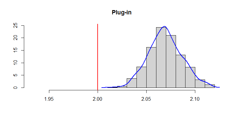
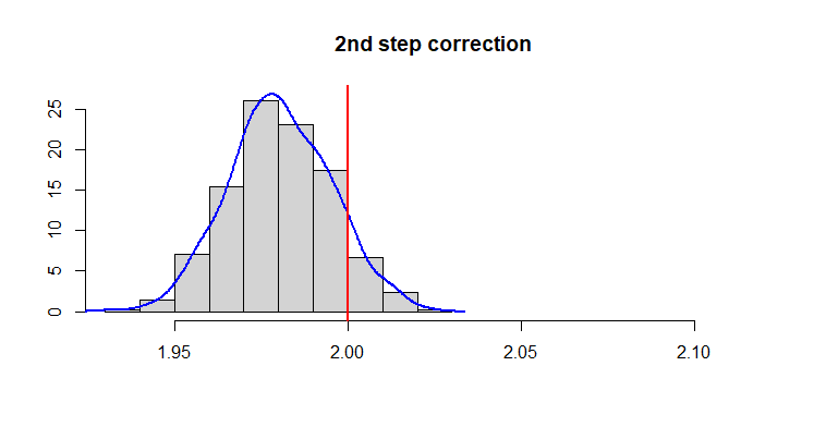
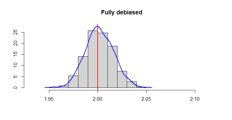
Figure 3: Distribution of the CASF estimators using a quadratic dictionary for a sample size of $n=10000$.

The tables highlight that the plug-in estimator suffers from severe asymptotic bias issues: coverage decreases rapidly, even if the confidence interval is constructed with correct standard errors. Indeed, Figure 3 shows that, for a sample size of $n=10000$, the distribution of plug-in estimators has almost zero mass near the true parameter $\theta_{0}=2$.

	Mean Absolute Bias			Standard Error			Coverage (95%)
n	PI	DR	LR	PI	DR	LR	PI	DR	LR
100	0.2764	0.1898	0.1957	0.1766	0.2003	0.2	0.5532	0.7534	0.7561
500	0.1462	0.0603	0.0527	0.0692	0.0709	0.0663	0.3794	0.8963	0.9327
1000	0.1214	0.0446	0.0374	0.0491	0.0488	0.0465	0.2329	0.8717	0.929
5000	0.079	0.0259	0.0161	0.0236	0.0212	0.0202	0.0437	0.737	0.9354
10000	0.0694	0.0209	0.0115	0.0172	0.0148	0.0143	0.0036	0.6533	0.9327

Table 2: CASF results for the dictionary including linear and quadratic terms.

Table 3 displays results for the dictionary that also includes interaction terms. The results are striking, as the Doubly Robust estimator that only accounts for the second step performs well. It is able to keep coverage at nominal levels, outperforming the fully debiased estimator. Nevertheless, the decrease in coverage is small: 1-2% for intermediate sample sizes ($n=500$ and $1000$) and 4-5% for large samples ($n=5000$ and $10000$). We believe that this fact rests on the dictionaries performing well to estimate the second step correction, but notably worst to estimate the more complex fist step correction. This result suggest that the complexity of the dictionary must be increased faster when accounting for the first step.

	Mean Absolute Bias			Standard Error			Coverage (95%)
n	PI	DR	LR	PI	DR	LR	PI	DR	LR
100	0.3447	0.3583	0.3857	0.179	0.3606	0.4054	0.9016	0.7969	0.806
500	0.1707	0.0997	0.1085	0.0693	0.1213	0.1359	0.7925	0.9481	0.9227
1000	0.1367	0.0635	0.0674	0.0488	0.0776	0.0849	0.5883	0.9372	0.9262
5000	0.0846	0.0259	0.0283	0.0229	0.0312	0.0349	0.1383	0.9372	0.8926
10000	0.0729	0.0173	0.0205	0.017	0.0207	0.0228	0.0337	0.9399	0.8926

Table 3: CASF results for the dictionary including linear, quadratic, and interaction terms.

7 Conclusion

We propose Automatic Locally Robust estimators for structural parameters in the presence of generated regressors. We show that the debiasing correction term can be decomposed into terms accounting for first step and second step estimation. Each of the first and second step IF depends on an additional nuisance parameter, which can be automatically estimated (i.e., estimated without finding their analytic shape).

We apply our results to construct Automatic Locally Robust estimators for the CASF under the control function assumption, see also Appendix A for the Average Partial Effects example in sample selection models. The analytic shape of the nuisance parameters in these two cases is particularly complex, as the moment conditions depend on the whole shape of the second step parameter (not only its pointwise value). Therefore, automatic estimation is particularly suited for these problems. We have shown that commonly used plug-in methods lead to highly biased inferences for the CASF. Doubly Robust and fully Locally Robust estimators correct the bias and deliver much more accurate inference in a complex setting with generated regressors.

Appendix A Partial effects in sample selection models

Example 13

We observe $W=(Y,D,Z)$ following the model $Y=Y^{\ast}D\equiv H(X,\varepsilon)D$, where $X$ is a component of $Z$, and we do not observe $Y^{\ast}$ when $D=0$. This is a very general setting for sample selection models. We do not know much about the selection, so this is given by $D=1\left[g_{0}\left(Z\right)-U\geq 0\right]$, where $U$ is uniformly distributed in $[0,1]\$. The unobserved errors $\varepsilon$ and $U$, though independent of $Z$, are correlated with each other (selection on unobservables). In this example, $V=g_{0}\left(Z\right)=\mathbb{E}[D|Z]$. Then, it can be shown that

$$\mathbb{E}[Y|Z] =\mathbb{E}[H(X,\varepsilon)1\left[g_{0}\left(Z\right)-U\geq 0\right]|Z]$$

$$=h_{0}(X,V).$$

This setting provides a nonparametric extension of the classical model of Heckman, (1979), where $H(X,\varepsilon)=X^{\prime}\beta_{0}+\varepsilon,$ $g_{0}\left(Z\right)=Z^{\prime}\gamma_{0}$, and the joint distribution of $(\varepsilon,U)$ is bivariate Gaussian.

As a parameter of interest consider the Average Partial Effects (APE) given, for simplicity of presentation for a one-dimensional continuous regressor, by

$$\theta_{0}=\mathbb{E}\left[\frac{\partial h_{0}}{\partial x}(X,V)\right].$$

The moment function identifying the APE is

$$m(w,g,h,\theta)=\left.\frac{\partial}{\partial s}h(s,g(z))\right\rvert_{s=x}-\theta.$$

This parameter is covered by Proposition 5 in Hahn and Ridder, (2019). However, the authors do not consider Locally Robust estimation. Here we propose a novel Locally Robust estimator for the APE which (i) is Doubly Robust to the second step and (ii) allows for ML first and second step estimators.

Let $\partial h(x,v)/\partial x$ denote the derivative of $h(x,v)$ w.r.t. its first argument at $(x,v)$. Let $\partial^{2}h(x,v)/\partial x\partial v$ denote the derivative w.r.t. both arguments at $(x,v)$. For the APE, we have that the moment function is linear in $h$. Thus:

$$D_{2}(w,h|g_{0},h_{0},\theta)=\frac{\partial h}{\partial x}(x,g_{0}(z)),$$

where we have already make explicit the dependence of $D_{2}$ on $(g_{0},h_{0},\theta)$. We can also linearize the moment condition in $g$ to obtain:

$$D_{1}(w,g|g_{0},h_{0},\alpha_{0},\theta) =\left\{D_{11}(d,z)+\frac{\partial}{\partial v}\left[\alpha_{02}(x,v)(y-h_{0}(x,v))\right]\right\}g(z),\text{ with }$$

$$D_{11}(d,z) \equiv\frac{\partial^{2}h_{0}}{\partial x\partial v}(x,g_{0}(z)).$$

The debias estimator for the APE is

$$\hat{\theta}=\frac{1}{n}\sum_{\ell=1}^{L}\sum_{i\in I_{\ell}}\frac{\partial\hat{h}_{\ell}}{\partial x}(X_{i},\hat{g}_{\ell}(Z_{i}))+\hat{\phi},$$

where, for the estimator $\hat{h}_{\ell}$, we can estimate its derivative w.r.t. $x$ by

$$\frac{\hat{h}_{\ell}}{\partial x}(x,v)\equiv\frac{\hat{h}_{\ell}(x+s_{n},v)-\hat{h}_{\ell}(x,v)}{s_{n}},$$

for a tuning parameter $s_{n}$. Alternatively, we can take advantage of a differentiable dictionary $(b_{j}(x,v))_{j=1}^{\infty}$, as described below.

To construct $\hat{\phi}$, we need to estimate $\alpha_{01}$ and $\alpha_{02}$. We propose automatic estimators for these nuisance parameters. We assume that $\partial h_{0}/\partial x$ and $\partial h_{0}/\partial v$ are differentiable, so we can interchange the order of differentiation.

Consider a dictionary $(b_{j})_{j=1}^{\infty}$ that is differentiable w.r.t. both $x$ and $v$. To Estimate $\hat{D}_{2\ell}$, we can compute $D_{2}(W_{i},b_{j}|\hat{g}_{\ell\ell^{\prime}},\hat{h}_{\ell\ell^{\prime}},\tilde{\theta}_{\ell\ell^{\prime}})$ for an observation $i\in I_{\ell^{\prime}}$ by

$$\frac{\partial b_{j}}{\partial x}(X_{i},\hat{g}_{\ell\ell^{\prime}}(Z_{i})).$$

This derivative can be found analytically for each atom. We can use this to obtain an automatic estimator of $\alpha_{02}$.

To construct $\hat{D}_{1\ell}$, we need to estimate $D_{1}(W_{i},c_{k}|\hat{g}_{\ell\ell^{\prime}},\hat{h}_{\ell\ell^{\prime}},\hat{\alpha}_{2\ell\ell^{\prime}},\tilde{\theta}_{\ell\ell^{\prime}})$ for an observation $i\in I_{\ell^{\prime}}$ and an arbitrary atom $c_{k}$ in a dictionary. The first term, $D_{11}(D_{i},Z_{i})$, can be estimated by

$$\left(\frac{\partial^{2}\mathbf{b}_{J}}{\partial x\partial v}(X_{i},\hat{g}_{\ell\ell^{\prime}}(Z_{i}))\right)^{\prime}\hat{\boldsymbol{\eta}}_{J},$$

in case that $h_{0}(x,v)$ is approximated by $\mathbf{b}_{J}(x,v)^{\prime}\hat{\boldsymbol{\eta}}_{J}$. An estimator of the second term, $\partial[\alpha_{02}(x,v)\cdot(y-h_{0}(x,v)]/\partial v$, is

$$\frac{\partial\mathbf{b}_{J}}{\partial v}(X_{i},\hat{g}_{\ell\ell^{\prime}}(Z_{i}))^{\prime}\hat{\boldsymbol{\rho}}_{J}\cdot\left[Y_{i}-\mathbf{b}_{J}(X_{i},\hat{g}_{\ell\ell^{\prime}}(Z_{i}))^{\prime}\hat{\boldsymbol{\eta}}_{J\ell\ell^{\prime}}\right]-\mathbf{b}_{J}(X_{i},\hat{g}_{\ell\ell^{\prime}}(Z_{i}))^{\prime}\hat{\boldsymbol{\rho}}_{J\ell\ell^{\prime}}\cdot\frac{\partial\mathbf{b}_{J}}{\partial v}(X_{i},\hat{g}_{\ell\ell^{\prime}}(Z_{i}))^{\prime}\hat{\boldsymbol{\eta}}_{J}$$

Appendix B Proofs of the results

Proof of (Proposition 3.1):

For the (differentiable) path $\tau\mapsto h(F_{\tau},g_{0})$, Assumption 3.1 implies

$$\frac{d}{d\tau}\bar{m}(g_{0},h(F_{\tau},g_{0}),\theta)=\frac{d}{d\tau}\mathbb{E}[D_{2}(W,h(F_{\tau},g_{0})].$$

This gives the linearization (LIN).

To find the shape of the IF, note that $\mathbb{E}[D_{2}(W,h)]$ is a linear and continuous functional in $L_{2}(X,V)$, a Hilbert space of square-integrable functions. Thus, by the Riesz Representation Theorem, there exists a $r_{2}$ such that $\mathbb{E}[D_{2}(W,h)]=\mathbb{E}[r_{2}(X,V)h(X,V)]$, with $V\equiv\varphi(D,Z,g_{0})$. Therefore:

$$\frac{d}{d\tau}\bar{m}(g_{0},h(F_{\tau},g_{0}),\theta)=\frac{d}{d\tau}\mathbb{E}[r_{2}(X,V)h(F_{\tau},g_{0})(X,V)],$$

where $h(F,g)(x,v)$ denotes $h(F,g)$ evaluated at $(x,v)$. This is Assumption 1 in Ichimura and Newey, (2022). Since Assumption 2 in that paper is satisfied in our setup, Proposition 1 in Ichimura and Newey, (2022) gives: $\phi_{2}(w,h_{0},\alpha_{02},\theta)=\alpha_{02}(d,z)\{y-h_{0}(x,\varphi(d,z,g_{0}))\}$. The parameter $\alpha_{02}$ is the $L_{2}$-projection of $r_{2}$ onto $\Delta_{2}(g_{0})$:

$${}\alpha_{02}=\operatornamewithlimits{argmin}_{\alpha\in\Delta_{2}(g_{0})}\mathbb{E}[(r_{2}(X,\varphi(D,Z,g_{0}))-\alpha(D,Z))^{2}].$$ (B.1)

This gives Point (IF).

Proof of (Lemma 3.1):

We proceed as in Hahn and Ridder, (2013, Lma. 1). Let $\tau\mapsto g_{\tau}$ be a differentiable path. For any function $\delta_{2}\in\Delta_{2}(g_{\tau})$, we have that

$$\mathbb{E}[\delta_{2}(X,V(g_{\tau}))\cdot\{Y-h(F_{0},g_{\tau})(X,V(g_{\tau}))\}]=0.$$

This is the orthogonality condition that defines $h(F_{0},g_{\tau})$ (it is equation (2.4) for $(F,g)=(F_{0},g_{\tau})$). If $\delta_{2}\in\Delta_{2}(g_{\tau})$ when $\tau<\varepsilon$, we can take derivatives in the above equation. Thus, applying the chain rule, we get

$$\frac{d}{d\tau}\mathbb{E}[\delta_{2}(X,V)\cdot h(F_{0},g_{\tau})(X,V)] =-\frac{d}{d\tau}\mathbb{E}[\delta_{2}(X,V)\cdot h_{0}(X,V(g_{\tau}))]$$

$$+\frac{d}{d\tau}\mathbb{E}\left[\delta_{2}(X,V(g_{\tau}))\cdot(Y-h_{0}(X,V))\right].$$

Proof of (Theorem 3.1):

We compute $d\bar{m}(g(F_{\tau}),h_{0},\theta)/d\tau$ and $d\bar{m}(g_{0},h(F_{0},g(F_{\tau})),\theta)/d\tau$ separately and then add them according to equation (3.2). By Assumptions 3.1 and 3.2, using the Riesz Representation Theorem, we have that for the differentiable paths $\tau\mapsto g(F_{\tau})$ and $\tau\mapsto h(F_{0},g(F_{\tau}))$:

$${}\frac{d}{d\tau}\bar{m}(g(F_{\tau}),h_{0},\theta)=\frac{d}{d\tau}\mathbb{E}[D_{11}(W,g(F_{\tau}))]=\frac{d}{d\tau}\mathbb{E}[r_{1}(Z)g(F_{\tau})(Z)]$$ (B.2)

and, being $V\equiv\varphi(D,Z,g_{0})$,

$$\frac{d}{d\tau}\bar{m}(g_{0},h(F_{0},g(F_{\tau})),\theta)=\frac{d}{d\tau}\mathbb{E}[D_{2}(W,h(F_{0},g(F_{\tau})))]=\frac{d}{d\tau}\mathbb{E}[r_{2}(X,V)h(F_{0},g(F_{\tau}))(X,V)].$$

In these equations, $g(F)(z)$ means $g(F)$ evaluated at $z$, and $h(F,g)(x,v)$ means $h(F,g)$ evaluated at $(x,v)$. By Assumption 3.3.b, $h(F_{0},g(F_{\tau}))\in\Delta_{2}(g_{0})$. This means that $h(F_{0},g(F_{\tau}))$ is orthogonal to $r_{2}-\alpha_{02}$ (since $\alpha_{02}$ is the $L_{2}$-projection of $r_{2}$ onto $\Delta_{2}(g_{0})$). Then, we can write:

$${}\frac{d}{d\tau}\bar{m}(g_{0},h(F_{0},g(F_{\tau})),\theta)=\frac{d}{d\tau}\mathbb{E}[\alpha_{02}(X,V)h(F_{0},g(F_{\tau}))(X,V)].$$ (B.3)

By Assumption 3.3.a we can apply Lemma 3.1 to the RHS of equation (B.3) to get:

$$\frac{d}{d\tau}\bar{m}(g_{0},h(F_{0},g(F_{\tau})),\theta) =\frac{d}{d\tau}\mathbb{E}[\alpha_{02}(X,V)h(F_{0},g(F_{\tau}))(X,V)]$$ (B.4)

$$=-\frac{d}{d\tau}\mathbb{E}[\alpha_{02}(X,V)h_{0}(X,\varphi(D,Z,g(F_{\tau})))]$$

$$+\frac{d}{d\tau}\mathbb{E}\left[\alpha_{02}(X,\varphi(D,Z,g(F_{\tau})))\cdot(Y-h_{0}(X,V))\right].$$

Under Assumption 3.4, the term in the second row can be linearized in $g(F_{\tau})$ as

$$\frac{d}{d\tau}\mathbb{E}[\alpha_{02}(X,V)h_{0}(X,\varphi(D,Z,g(F_{\tau})))] =\mathbb{E}\left[\frac{d}{d\tau}\{\alpha_{02}(X,V)h_{0}(X,\varphi(D,Z,g(F_{\tau})))\}\right]$$

$$=\mathbb{E}\left[\alpha_{02}(X,V)\frac{\partial h_{0}}{\partial v}(X,V)\frac{d}{d\tau}\varphi(D,Z,g(F_{\tau}))\right]$$

$$=\mathbb{E}\left[\alpha_{02}(X,V)\frac{\partial h_{0}}{\partial v}(X,V)\frac{d}{d\tau}D_{\varphi}g(F_{\tau})(D,Z)\right]$$

$$=\frac{d}{d\tau}\mathbb{E}\left[\alpha_{02}(X,V)\frac{\partial h_{0}}{\partial v}(X,V)D_{\varphi}g(F_{\tau})(D,Z)\right],$$

where $D_{\varphi}g(d,z)$ denotes $D_{\varphi}g$ evaluated at $(d,z)$. We have assumed that derivatives and expectations can be interchanged (we may impose some regularity conditions on $H$ such that this is possible). We can equivalently linearize the term in the third row of equation (B.4) to get

$$\frac{d}{d\tau}\mathbb{E}\left[\alpha_{02}(X,\varphi(D,Z,g(F_{\tau})))\cdot(Y-h_{0}(X,V))\right]=\frac{d}{d\tau}\mathbb{E}\left[(Y-h_{0}(X,V))\frac{\partial\alpha_{02}}{\partial v}(X,V)D_{\varphi}g(F_{\tau})(D,Z)\right].$$

Pluging in these results back in equation (B.4):

$$\frac{d}{d\tau}\bar{m}(g_{0},h(F_{0},g(F_{\tau})),\theta) =\frac{d}{d\tau}\mathbb{E}\left[\left\{-\alpha_{02}(X,V)\frac{\partial h_{0}}{\partial v}(X,V)\right.\right.$$ (B.5)

$$\left.\left.+(Y-h_{0}(X,V))\frac{\partial\alpha_{02}}{\partial v}(X,V)\right\}D_{\varphi}g(F_{\tau})(D,Z)\right]$$

$$=\mathbb{E}\left[\left.\frac{\partial}{\partial v}\left\{\alpha_{02}(X,v)\cdot(Y-h_{0}(X,v))\right\}\right\rvert_{v=V}D_{\varphi}g(F_{\tau})(D,Z)\right].$$

Since $D_{\varphi}$ is linear in $g$, the function inside the expectation in the RHS is linear in $g$. We now use equation (3.2) to combine the results in equations (B.2) and (B.5). This gives:

$$\frac{d}{d\tau}\bar{m}(g(F_{\tau}),h(F_{0},g(F_{\tau})),\theta)=\frac{d}{d\tau}\mathbb{E} \biggl{[}D_{11}(W,g(F_{\tau}))$$

$$\left.\left.+\frac{\partial}{\partial v}\left\{\alpha_{02}(X,v)\cdot(Y-h_{0}(X,v))\right\}\right\rvert_{v=V}D_{\varphi}g(F_{\tau})(D,Z)\right],$$

which gives the linearization result of the Theorem (LIN).

To find the shape of the IF, note that the adjoint $D_{\varphi}^{*}$ of $D_{\varphi}$ is defined by the equation $\mathbb{E}[\delta(D,Z)D_{\varphi}g(D,Z)]=\mathbb{E}[D_{\varphi}^{*}\delta(Z)g(Z)]$. Therefore, by the Law of Iterated Expectations in equation (B.5), noting that $V\equiv\varphi(D,Z,g_{0})$ is a function of $(D,Z)$:

$$\frac{d}{d\tau}\bar{m}(g_{0},h(F_{0},g(F_{\tau})),\theta) =\frac{d}{d\tau}\mathbb{E}\left[\mathbb{E}\left[\left.\left.\frac{\partial}{\partial v}\left\{\alpha_{02}(X,v)\cdot(Y-h_{0}(X,v))\right\}\right\rvert_{v=V}D_{\varphi}g(F_{\tau})(D,Z)\right\lvert D,Z\right]\right]$$

$$=\mathbb{E}[\nu(D,Z)D_{\varphi}g(F_{\tau})(D,Z)]=\mathbb{E}[D_{\varphi}^{*}\nu(Z)g(F_{\tau})(Z)],$$

with

$$\nu(d,z)\equiv\left.\frac{\partial}{\partial v}\left\{\alpha_{02}(x,v)\cdot(\mathbb{E}[Y|D=d,Z=z]-h_{0}(x,v))\right\}\right\rvert_{v=\varphi(d,z,g_{0})}.$$

Again, we can use equation (3.2) to combine this last result with that in equation (B.2):

$$\frac{d}{d\tau}\bar{m}(g(F_{\tau}),h(F_{0},g(F_{\tau})),\theta)=\frac{d}{d\tau}\mathbb{E}[\{r_{1}(Z)+D_{\varphi}^{*}\nu(Z)\}g(F_{\tau})(Z)].$$

This is Assumption 1 in Ichimura and Newey, (2022). Since Assumption 2 in that paper is satisfied in our setup, Proposition 1 in Ichimura and Newey, (2022) gives the shape of the IF: $\phi_{1}(w,g_{0},\alpha_{01},\theta)=\alpha_{01}(z)\cdot\{d-g_{0}(z)\}$. The parameter $\alpha_{01}$ is the $L_{2}$-projection:

$${}\alpha_{01}=\operatornamewithlimits{argmin}_{\alpha\in\Delta_{1}}\mathbb{E}[(\tilde{\nu}(Z)-\alpha(Z))^{2}],$$ (B.6)

where $\tilde{\nu}=r_{1}+D_{\varphi}^{*}\nu$.

Proof of (Proposition 3.2):

Start with the non-parametric case. Let $v(g)\equiv\varphi(d,z,g)$ By the triangle inequality (applied to the $L_{2}(W)$-norm):

$$\left(\int\alpha_{02}(x,v(g_{\tau}))^{2}dF_{0}(w)\right)^{1/2} \leq\left(\int\alpha_{02}(x,v(g_{0}))^{2}dF_{0}(w)\right)^{1/2}$$

$$+\left(\int\left[\alpha_{02}(x,v(g_{\tau}))-\alpha_{02}(x,v(g_{0}))\right]^{2}dF_{0}(w)\right)^{1/2}$$

The fist quantity in the RHS is finite since $\alpha_{02}\in L_{2}(X,V)$. For quantity in the second row, by the MVT and Hadamard differentiability of $\varphi$:

$$\left(\int\left(\alpha_{02}(x,v(g_{\tau}))-\alpha_{02}(x,v)\right)^{2}dF_{0}(w)\right)^{1/2}\leq C\lVert\varphi(g_{\tau})-\varphi(g_{0})\rVert$$

$$=C\lVert\varphi(g_{\tau})-\varphi(g_{0})-D\varphi(g_{\tau}-g_{0})+D\varphi(g-g_{0})\rVert\leq C\left(\lVert D\varphi\rVert\cdot\lVert g_{\tau}-g_{0}\rVert+o(\lVert g_{\tau}-g_{0}\rVert)\right),$$

where $C$ is the bound of $\partial\alpha_{02}/\partial v$ and, in some abuse of notation, $\lVert\cdot\rVert$ denotes the norm in the corresponding space. Let $\varepsilon$ be such that $o(\lVert g_{\tau}-g_{0}\rVert)\leq\lVert g_{\tau}-g_{0}\rVert$. For $\tau<\varepsilon$:

$$\left(\int\left(\alpha_{02}(x,v(g_{\tau}))-\alpha_{02}(x,v)\right)^{2}dF_{0}(w)\right)^{1/2}\leq C(\lVert D\varphi\rVert+1)\lVert g_{\tau}-g_{0}\rVert,$$

which is finite since $\tau\mapsto g_{\tau}$ is a differentiable path in $\Delta_{1}$.

For the partly linear case, where $\alpha_{02}(x,v)=\beta_{0}^{\prime}x+\kappa_{0}(v)$, simply note that

$$\frac{\partial\alpha_{02}}{\partial v}(x,v)=\frac{\partial\kappa_{0}}{\partial v}(x,v).$$

Thus, $\partial\kappa_{0}/\partial v$ is bounded and we can proceed as above to show that $\int\kappa_{0}(v(g_{\tau}))^{2}dF_{0}(w)$ is finite.

Proof of (Proposition 3.3):

We start with the non-parametric case. Throughout the proof, we call $h_{\tau}\equiv h(F_{0},g_{\tau})$. We note that $h_{\tau}\in\Delta_{2}(g_{0})=L_{2}(X,V)$ if and only if $\int h_{\tau}(x,v)^{2}dF_{xv}^{0}(x,v)<\infty$. Under the conditions in the statement of the proposition, by Cauchy-Schwarz’ inequality:

$$\int h_{\tau}(x,v)^{2}dF_{xv}^{0}(x,v)=\int h_{\tau}(x,v)^{2}\nu_{\tau}(x,v)dF_{xv}^{\tau}(x,v)\leq\int h_{\tau}(x,v)^{4}dF_{xv}^{\tau}(x,v)+\int\nu_{\tau}(x,v)^{2}dF_{xv}^{\tau}(x,v).$$

Furthermore, since $h_{\tau}(X,V(g_{\tau}))=\mathbb{E}[Y|X,V(g_{\tau})]$, by conditional Jensen’s inequality and the Law of Iterated Expectations

$$\int h_{\tau}(x,v)^{4}dF_{xv}^{\tau}(x,v)=\mathbb{E}[\mathbb{E}[Y|X,V(g_{\tau})]^{4}]\leq\mathbb{E}[\mathbb{E}[Y^{4}|X,V(g_{\tau})]]=\mathbb{E}[Y^{4}]<\infty.$$

Also, since the Radon-Nikodym density of $F_{xv}^{\tau}$ w.r.t. $F_{xv}^{0}$ is $\nu_{\tau}(x,v)^{-1}$ (Shao,, 2003, Prop. 1.7):

$$\int\nu_{\tau}(x,v)^{2}dF_{xv}^{\tau}(x,v)=\int\nu_{\tau}(x,v)dF_{xv}^{0}(x,v)=\mathbb{E}[\nu_{\tau}(X,V)]<\infty.$$

For the partly linear case we need to show that $\int\kappa_{\tau}(v)^{2}dF_{v}^{0}(v)<\infty$. We can proceed as above to get:

$$\int\kappa_{\tau}(v)^{2}dF_{v}^{0}(v)\leq\int\kappa_{\tau}(v)^{4}dF_{v}^{\tau}(v)+\mathbb{E}[\nu_{\tau}(V)],$$

where the second quantity in the RHS is finite by assumption. In the partly linear model we have that $\mathbb{E}[Y|V(g_{\tau})]=\beta_{\tau}^{\prime}\mathbb{E}[X|V(g_{\tau})]+\kappa_{\tau}(V(g_{\tau}))$. Therefore,

$$\int\kappa_{\tau}(v)^{4}dF_{v}^{\tau}(v)=\mathbb{E}[\kappa_{\tau}(V(g_{\tau}))^{4}]=\mathbb{E}[\mathbb{E}[Y-\beta_{\tau}^{\prime}X|V(g_{\tau})]^{4}]\leq\mathbb{E}[(Y-\beta_{\tau}^{\prime}X)^{4}].$$

This is finite if the expectation of the fourth-order cross-products between $Y$ and $X$ is finite.

The asymptotic normality and consistent estimation of the asymptotic variance result in Theorem 5.1 relies on the following lemma:

Lemma B.1

Consider Assumptions 3.4, 5.3, 5.4.a, and 5.9. Let $r,\xi>0$. Then, for $\tilde{h}_{\ell}(w)\equiv\hat{h}_{\ell}(x,\varphi(d,z,\hat{g}_{\ell}))$ and $\tilde{\alpha}_{2\ell}(w)\equiv\hat{\alpha}_{2\ell}(x,\varphi(d,z,\hat{g}_{\ell}))$:

$$\lVert\hat{h}_{\ell}-h_{0}\rVert_{2} =O_{p}(n^{-r})\Rightarrow\lVert\tilde{h}_{\ell}-h_{0}\rVert_{2}=O_{p}(n^{-r}),\text{ and }$$

$$\lVert\hat{\alpha}_{2\ell}-\alpha_{02}\rVert_{2} =o_{p}(n^{\xi}n^{-r/2})\Rightarrow\lVert\tilde{\alpha}_{2\ell}-\alpha_{02}\rVert_{2}=o_{p}(n^{\xi}n^{-r/2}).$$

Proof of (Lemma B.1):

Recall that $\hat{h}_{\ell}(x,v)\equiv\mathbf{b}_{J}(x,v)^{\prime}\hat{\boldsymbol{\eta}}_{J}$ and $\hat{\alpha}_{2\ell}(x,v)\equiv\mathbf{b}_{J}(x,v)^{\prime}\hat{\boldsymbol{\rho}}_{J}$. We show that

$$\lVert\tilde{h}_{\ell}-\hat{h}_{\ell}\rVert_{2}=O_{p}(n^{-r}).$$

The conclusion for $\tilde{\alpha}_{2\ell}$ follows the same reasoning.

Let $\tilde{b}_{j}(w)\equiv b_{j}(w,\varphi(d,z,\hat{g}_{\ell}))$. By the triangle inequality $\lVert\hat{h}_{\ell}-\hat{h}_{\ell}\rVert_{2}\leq\sum_{j=1}^{J}|\hat{\eta}_{j}|\lVert\tilde{b}_{j}-b_{j}\rVert_{2}$. Moreover, by the Mean Value Theorem and Assumption 5.9.b,

$$\lVert\tilde{b}_{j}-b_{j}\rVert_{2}^{2}=\int(b_{j}(x,\varphi(d,z,\hat{g}_{\ell}))-b_{j}(x,v))^{2}dF_{0}(w)\leq\kappa^{2}\lVert\varphi(\cdot,\cdot,\hat{g}_{\ell})-\varphi(\cdot,\cdot,g_{0})\rVert_{2}^{2}.$$

Then, $\sup_{j\leq J}\lVert\tilde{b}_{j}-b_{j}\rVert_{2}\leq\kappa\lVert\varphi(\cdot,\cdot,\hat{g}_{\ell})-\varphi(\cdot,\cdot,g_{0})\rVert_{2}$. Also, since $\varphi$ is Hadamard differentiable (Assumption 3.4): $\lVert\varphi(\cdot,\cdot,\hat{g}_{\ell})-\varphi(\cdot,\cdot,g_{0})-D_{\varphi}(\hat{g}_{\ell}-g_{0})\rVert_{2}=o_{p}(\lVert\hat{g}_{\ell}-g_{0}\rVert)$ and $\lVert D_{\varphi}(\hat{g}_{\ell}-g_{0})\rVert_{2}\leq C\lVert\hat{g}_{\ell}-g_{0}\rVert_{2}$ (see Yamamuro,, 1974, Result 1.2.6). Thus, by the triangle inequality:

$$\sup_{j\leq J}\lVert\tilde{b}_{j}-b_{j}\rVert_{2}\leq\kappa C\lVert\hat{g}_{\ell}-g_{0}\rVert_{2}+o_{p}(\lVert\hat{g}_{\ell}-g_{0}\rVert_{2}).$$

Now, Assumption 5.3 allows us to apply Lemma A9 in Chernozhukov et al., 2022b to get $\sum_{j=1}^{J}|\hat{\eta_{j}}|=O_{p}(1)$. Therefore, if Assumption 5.4.a holds,

$$\lVert\hat{h}_{\ell}-\hat{h}_{\ell}\rVert_{2} \leq\sum_{j=1}^{J}|\hat{\eta}_{j}|\lVert\tilde{b}_{j}-b_{j}\rVert_{2}\leq\left(\sum_{j=1}^{J}|\hat{\eta}_{j}|\right)\left(\kappa C\lVert\hat{g}_{\ell}-g_{0}\rVert_{2}+o_{p}(\lVert\hat{g}_{\ell}-g_{0}\rVert_{2})\right)$$ (B.7)

$$=O_{p}(1)\cdot[O_{p}(n^{-r})+o_{p}(n^{-r})]=O_{p}(n^{-r}).$$

The conclusion for $\lVert\tilde{h}_{\ell}-h_{0}\rVert_{2}$ follows directly from equation (B.7) and the triangle inequality. The conclusion for $\lVert\tilde{\alpha}_{2\ell}-\alpha_{02}\rVert_{2}$ follows equally, taking into account that $O_{p}(n^{-r})=o_{p}(n^{\xi}n^{-r/2})$ for $\xi>0$.

Proof of (Theorem 5.1):

We start with asymptotic normality of $\sqrt{n}(\hat{\theta}-\theta_{0})$. The proof follows standard GMM techniques and Theorem 9 in Chernozhukov et al., 2022b . A relevant deviation from the previous results is that the estimators are evaluated at the generated regressor. Lemma B.1 allows to deal with that situation.

The cornerstone of the result is Lemma 8 in Chernozhukov et al., 2022a , CEINR in what follows, which states that:

$$\sqrt{n}\hat{\psi}(\theta_{0})=\frac{1}{\sqrt{n}}\sum_{i=1}^{n}\psi(W_{i},g_{0},h_{0},\alpha_{0},\theta_{0})+o_{p}(1)$$ (B.8)

under some conditions. We will apply Lemma 8 to a modified expansion of the difference between $\hat{\psi}(\theta_{0})$ and $n^{-1/2}\sum_{i=1}^{n}\psi(W_{i},g_{0},h_{0},\alpha_{0},\theta_{0})$ that allows to deal with estimators evaluated at the generated regressor.

Consider first that equation (B.8) holds for each component of $\hat{\psi}$. Consistency of $\hat{\theta}$ follows under standard conditions that guarantee uniform convergence of $\hat{\psi}(\theta)^{\prime}\hat{\Upsilon}\hat{\psi}(\theta)$ in $\Theta$ (c.f. Wooldridge,, 2010, Th. 14.1). These conditions will follow from Assumption 5.8 if $\Theta$ is compact. Moreover, by Assumptions 5.4.a and 5.8.a we can apply the Mean Value Theorem to get

$$\sqrt{n}\left(\hat{\psi}(\hat{\theta})-\hat{\psi}\left(\theta_{0}\right)\right)=\sqrt{n}\frac{\partial\hat{\psi}}{\partial\theta}(\bar{\theta})\cdot(\hat{\theta}-\theta_{0})$$

for $\bar{\theta}$ a point between $\theta_{0}$ and $\hat{\theta}$ (that is $\bar{\theta}\xrightarrow{P}\theta_{0}$). Then, if equation (B.8) holds:

$$\sqrt{n}\frac{\partial\hat{\psi}}{\partial\theta}(\bar{\theta})\cdot(\hat{\theta}-\theta_{0})=\frac{1}{\sqrt{n}}\sum_{i=1}^{n}\psi(W_{i},g_{0},h_{0},\alpha_{0},\theta_{0})+\sqrt{n}\hat{\psi}(\hat{\theta})+o_{p}(1).$$ (B.9)

Now, note that

$$\frac{\partial\hat{\psi}}{\partial\theta}(\theta) =\frac{\partial}{\partial\theta}\left(\frac{1}{n}\sum_{\ell=1}^{L}\sum_{i\in I_{\ell}}\left[m(W_{i},\hat{g}_{\ell},\hat{h}_{\ell},\theta)+\phi(W_{i},\hat{g}_{\ell},\hat{h}_{\ell},\hat{\alpha}_{\ell},\tilde{\theta}_{\ell})\right]\right)$$

$$=\frac{1}{n}\sum_{\ell=1}^{L}\sum_{i\in I_{\ell}}\frac{\partial m}{\partial\theta}(W_{i},\hat{g}_{\ell},\hat{h}_{\ell},\theta)$$

Then, since Assumptions 5.4.a and 5.8, on top of $\hat{\theta}\xrightarrow{P}\theta_{0}$, guarantee that we can apply Lemma E2 in CEINR, we have that $\partial\hat{\psi}(\hat{\theta})/\partial\theta\xrightarrow{P}M$, so it is bounded in probability. Therefore, since $\hat{\Upsilon}$ is also $O_{p}(1)$, equation (B.9) implies

$$\frac{\partial\hat{\psi}}{\partial\theta}(\hat{\theta})^{\prime}\hat{\Upsilon}\frac{\partial\hat{\psi}}{\partial\theta}(\bar{\theta})\cdot\sqrt{n}(\hat{\theta}-\theta_{0}) =\frac{\partial\hat{\psi}}{\partial\theta}(\hat{\theta})^{\prime}\hat{\Upsilon}\cdot\frac{1}{\sqrt{n}}\sum_{i=1}^{n}\psi(W_{i},g_{0},h_{0},\alpha_{0},\theta_{0})$$

$$+\sqrt{n}\frac{\partial\hat{\psi}}{\partial\theta}(\hat{\theta})^{\prime}\hat{\Upsilon}\hat{\psi}(\hat{\theta})+o_{p}(1).$$

Thus, since $(\partial\hat{\psi}(\hat{\theta})/\partial\theta)^{\prime}\hat{\Upsilon}\hat{\psi}(\hat{\theta})=0$ is the first-order condition for the minimization problem in equation (4.3), $\partial\hat{\psi}(\bar{\theta})/\partial\theta\xrightarrow{P}M$ (by Lemma E2 in CEINR), and $M^{\prime}\Upsilon M$ is non-sigular:

$$\sqrt{n}(\hat{\theta}-\theta_{0})=(M^{\prime}\Upsilon M)^{-1}\frac{1}{\sqrt{n}}\sum_{i=1}^{n}\psi(W_{i},g_{0},h_{0},\alpha_{0},\theta_{0})+o_{p}(1).$$

Then, the asymptotic normality result follows from $n^{-1/2}\sum_{i=1}^{n}\psi(W_{i},g_{0},h_{0},\alpha_{0},\theta_{0})\xrightarrow{D}N(0,\Psi)$.

It remains to verify the assumptions for Lemma 8 in CEINR, so that equation (B.8) holds for each component of $\hat{\psi}$. First, to handle estimators evaluated at the generated regressor, we provide a modified expansion of the difference between $\hat{\psi}(\theta_{0})$ and $n^{-1/2}\sum_{i=1}^{n}\psi(W_{i},g_{0},h_{0},\alpha_{0},\theta_{0})$. Let $\bar{\phi}(w,\bar{v},g,h,\alpha)\equiv\alpha_{1}(z)\cdot(d-g(z))+\alpha_{2}(x,\bar{v})\cdot(y-h(x,\varphi(d,z,g)))$, which makes explicity that $\alpha_{2}$ is evaluated at $(x,\bar{v})$. Then, being $\hat{\psi}_{i\ell}(\theta)$ given by equation (4.2), we have that $\hat{\psi}_{i\ell}(\theta_{0})-\psi(W_{i},g_{0},h_{0},\alpha_{0},\theta_{0})=\hat{R}_{1i\ell}+\hat{R}_{2i\ell}+\hat{R}_{3i\ell}+\hat{\Delta}_{i\ell}$, where

$$\hat{R}_{1i\ell} \equiv m(W_{i},\hat{g}_{\ell},\hat{h}_{\ell},\theta_{0})-m(W_{i},g_{0},h_{0},\theta_{0}),$$ (B.10)

$$\hat{R}_{2i\ell} \equiv\bar{\phi}(W_{i},\varphi(D_{i},Z_{i},g_{0}),\hat{g}_{\ell},\hat{h}_{\ell},\alpha_{0})-\phi(W_{i},g_{0},h_{0},\alpha_{0},\theta_{0}),$$

$$\hat{R}_{3i\ell} \equiv\bar{\phi}(W_{i},\varphi(D_{i},Z_{i},\hat{g}_{\ell}),g_{0},h_{0},\hat{\alpha}_{\ell})-\phi(W_{i},g_{0},h_{0},\alpha_{0},\theta_{0}),$$

$$\hat{\Delta}_{i\ell} \equiv\phi(W_{i},\hat{g}_{\ell},\hat{h}_{\ell},\hat{\alpha}_{\ell},\tilde{\theta}_{\ell})-\bar{\phi}(W_{i},\varphi(D_{i},Z_{i},g_{0}),\hat{g}_{\ell},\hat{h}_{\ell},\alpha_{0}),\text{ and }$$

$$-\bar{\phi}(W_{i},\varphi(D_{i},Z_{i},\hat{g}_{\ell}),g_{0},h_{0},\hat{\alpha}_{\ell})+\phi(W_{i},g_{0},h_{0},\alpha_{0},\theta_{0}).$$

We will apply Lemma 8 in CEINR to this expansion.

Following Chernozhukov et al., 2022b , we begin by providing rates for estimation of $\alpha_{01}$ and $\alpha_{02}$. Assumption 5.2 allows us to apply Lemma A10 in Chernozhukov et al., 2022b to get $\lVert\hat{B}_{\ell}-\mathbb{E}[\mathbf{b}_{J}(X,V)\mathbf{b}_{J}(X,V)^{\prime}]\rVert_{\infty}=O_{p}(\sqrt{\log(J)/n})$ and $\lVert\hat{C}_{\ell}-\mathbb{E}[\mathbf{c}_{K}(Z)\mathbf{c}_{K}(Z)^{\prime}]\rVert_{\infty}=O_{p}(\sqrt{\log(K)/n})$. The fact that Assumption 5.5.b imposes a polynomial rate on $J$ and $K$ then implies that $O_{p}(\sqrt{\log(J)/n})=O_{p}(n^{-r})$ and $O_{p}(\sqrt{\log(K)/n})=O_{p}(n^{-r})$, since $r<1/2$ (Assumption 5.4). This, on top of Assumptions 5.1, 5.3, 5.4.b, and 5.5, means that we can apply Theorem 2 in Chernozhukov et al., 2022b to get:

$$\lVert\hat{\alpha}_{1\ell}-\alpha_{01}\rVert_{2}=o_{p}(n^{\xi}n^{-r/2})\text{ and }\lVert\hat{\alpha}_{2\ell}-\alpha_{02}\rVert_{2}=o_{p}(n^{\xi}n^{-r/2})$$

for any $\xi>0$. We choose a $\xi$ satisfying $0<\xi<(3r-1)/2<r/2$, which is possible since, by Assumption 5.4, $r\in(1/3,1/2)$. This guarantees that

$$\lVert\hat{\alpha}_{1\ell}-\alpha_{01}\rVert_{2}=o_{p}(1)\text{ and }\lVert\hat{\alpha}_{2\ell}-\alpha_{02}\rVert_{2}=o_{p}(1);\text{ and }$$ (B.11)

$$\sqrt{n}\lVert\hat{\alpha}_{1\ell}-\alpha_{01}\rVert_{2}\lVert\hat{g}-g_{0}\rVert_{2}=o_{p}(1)\text{ and }\sqrt{n}\lVert\hat{\alpha}_{2\ell}-\alpha_{02}\rVert_{2}\lVert\hat{h}_{\ell}-h_{0}\rVert=o_{p}(1),$$ (B.12)

where the last line follows from Assumption 5.4.a.

We now check Assumption 1 in CEINR. Assumption 1.i is identical to Assumption 5.6.a and 5.6.b. To show the remaining points, define $\tilde{h}_{\ell}(w)\equiv\hat{h}_{\ell}(x,\varphi(d,z,\hat{g}_{\ell}))$ and $\tilde{\alpha}_{2\ell}(w)\equiv\hat{\alpha}_{2\ell}(x,\varphi(d,z,\hat{g}_{\ell}))$. Note also that by Assumptions 5.2 and 5.3.a:

$$|\alpha_{01}(Z)| \leq\sum_{k=1}^{\infty}|\beta_{k}||c_{k}(Z)|\leq\sup_{k\in\mathbb{N}}|c_{k}(Z)|\cdot\sum_{k=1}^{\infty}|\beta_{k}|\equiv\kappa_{1}<\infty\text{ and }$$

$$|\alpha_{02}(X,V)| \leq\sum_{j=1}^{\infty}|\rho_{j}||b_{j}(X,V)|\leq\sup_{j\in\mathbb{N}}|b_{j}(X,V)|\cdot\sum_{j=1}^{\infty}|\rho_{j}|\equiv\kappa_{2}<\infty.$$

Thus, by the triangle inequality, being $v\equiv\varphi(d,z,g_{0})$:

$$\int\left[\bar{\phi}(w,\varphi(d,z,g_{0}),\hat{g}_{\ell},\hat{h}_{\ell},\alpha_{0})-\phi(w,g_{0},h_{0},\alpha_{0},\theta_{0})\right]^{2}dF_{0}(w)\leq\int\alpha_{01}(z)^{2}\left[\hat{g}_{\ell}(z)-g_{0}(z)\right]^{2}dF_{0}(w)$$

$$+\int\alpha_{02}(x,v)^{2}\left[\tilde{h}_{\ell}(w)-h_{0}(x,v)\right]^{2}dF_{0}(w)$$

$$\leq\kappa_{1}^{2}\lVert\hat{g}_{\ell}-g_{0}\rVert_{2}^{2}+\kappa_{2}^{2}\lVert\tilde{h}_{\ell}-h_{0}\rVert_{2}^{2}.$$

Assumption 1.ii in CEINR follows from the above display, Assumption 5.4.a, and Lemma B.1.

Also, calling $\kappa_{3},\kappa_{4}<\infty$ to the bounds given by Assumption 5.6.d:

$$\int\left[\bar{\phi}(w,\varphi(d,z,\hat{g}_{\ell}),g_{0},h_{0},\hat{\alpha}_{\ell})-\phi(w,g_{0},h_{0},\alpha_{0},\theta_{0})\right]^{2}dF_{0}(w)\leq\int\left[d-g_{0}(z)\right]^{2}\left[\hat{\alpha}_{1\ell}(z)-\alpha_{01}(z)\right]^{2}dF_{0}(w)$$

$$+\int\left[y-h_{0}(x,v)\right]^{2}\left[\tilde{\alpha}_{2\ell}(w)-\alpha_{02}(x,v)\right]^{2}dF_{0}(w)$$

$$\leq\kappa_{3}^{2}\lVert\hat{\alpha}_{1\ell}-\alpha_{01}\rVert_{2}^{2}+\kappa_{4}^{2}\lVert\tilde{\alpha}_{2\ell}-\alpha_{02}\rVert_{2}^{2},$$

Thus, Assumption 1.iii in CEINR follows from the above display, equation (B.11), and Lemma B.1.

We now move to check Assumption 2 in CEINR. In particular, we show that 2.iii holds. We have that

$$\hat{\Delta}_{i\ell}=[\hat{\alpha}_{1\ell}(Z_{i})-\alpha_{01}(Z_{i})]\cdot[\hat{g}_{\ell}(Z_{i})-g_{0}(Z_{i})]+[\tilde{\alpha}_{2\ell}(W_{i})-\alpha_{02}(X_{i},V_{i})]\cdot[\tilde{h}_{\ell}(W_{i})-h_{0}(X_{i},V_{i})].$$

Thus, as in Chernozhukov et al., 2022b (, proof of Th. 9), an application of the Cauchy-Schwarz, conditional Markov, and triangle inequalities leads to:

$$\left|\frac{1}{\sqrt{n}}\sum_{i\in I_{\ell}}\hat{\Delta}_{i\ell}\right|=O_{p}(\sqrt{n}\lVert\hat{\alpha}_{1\ell}-\alpha_{01}\rVert_{2}\lVert\hat{g}_{\ell}-g_{0}\rVert_{2})+O_{p}(\sqrt{n}\lVert\tilde{\alpha}_{2\ell}-\alpha_{01}\rVert_{2}\lVert\tilde{h}_{\ell}-h_{0}\rVert_{2}).$$

Thus, by equation (B.12) and Lemma B.1, Assumption 2.iii in CEINR is satisfied.

To see that Assumption 3.iii in CEINR holds, note that by Assumptions 3.1-3.4: $\mathbb{E}[D_{1}(W,g))]=\mathbb{E}[\alpha_{01}(Z)g(Z)]$ and $\mathbb{E}[D_{2}(W,h(\cdot,\varphi(\cdot,\cdot,g)))]=\mathbb{E}[\alpha_{02}(X,V)h(X,\varphi(D,Z,g))]$. The last equality also uses Assumption 5.9.c. Moreover, $D-g_{0}(Z)$ and $Y-h_{0}(X,V)$ are orthogonal to $\Delta_{1}$ and $\Delta_{2}(g_{0})$, respectively. Then,

$$\mathbb{E}[\bar{\phi}(W,\varphi(D,Z,g_{0}),g,h,\alpha_{0})] =\mathbb{E}[\alpha_{01}(Z)(g_{0}(Z)-g(Z))]+\mathbb{E}[\alpha_{02}(X,V)(h_{0}(X,V)-h(X,\varphi(D,Z,g)))]$$

$$=-\mathbb{E}[D_{1}(W,g-g_{0})]-\mathbb{E}[D_{2}(W,h(\cdot,\varphi(\cdot,\cdot,g))-h_{0})].$$

Thus, by Assumption 5.7, for $\lVert g-g_{0}\rVert_{2}<\varepsilon$ and $\lVert h-h_{0}\rVert_{2}<\varepsilon$:

$$\left|\mathbb{E}[m(W,g,h,\alpha_{0},\theta_{0})+\bar{\phi}(W,\varphi(D,Z,g_{0}),g,h,\alpha_{0})]\right|$$

$$=\left|\mathbb{E}\left[m(W,g,h,\theta_{0})-m(W,g_{0},h_{0},\theta_{0})-D_{1}(W,g-g_{0})-D_{2}(W,h(\cdot,\varphi(\cdot,\cdot,g))-h_{0})\right]\right|$$

$$\leq C\left(\lVert g-g_{0}\rVert_{2}^{2}+\lVert h(\cdot,\varphi(\cdot,\cdot,g))-h_{0}\rVert_{2}^{2}\right).$$

The above display, on top of Assumption 5.4.a and Lemma B.1, gives Assumption 3.iii in CEINR for the functional $(g,h)\mapsto\mathbb{E}[m(W,g,h,\alpha_{0},\theta_{0})+\bar{\phi}(W,\varphi(D,Z,g_{0}),g,h,\alpha_{0})]$.

To conclude, we verify that Lemma 8 in CEINR can be applied to our modified expansion. Being $I_{\ell}^{c}$ all observations not in $I_{\ell}$, note that

$$\mathbb{E}[\hat{R}_{1i\ell}+\hat{R}_{2i\ell}|I_{\ell}^{c}] =\mathbb{E}[m(W,\hat{g}_{\ell},\hat{h}_{\ell},\alpha_{0},\theta_{0})+\bar{\phi}(W,\varphi(D,Z,g_{0}),\hat{g}_{\ell},\hat{h}_{\ell},\alpha_{0})|I_{\ell}^{c}]\text{ and }$$

$$\mathbb{E}[\hat{R}_{3i\ell}|I_{\ell}^{c}] =0.$$

The last equation follows from orthogonality of $D-g_{0}(Z)$ and $Y-h_{0}(X,V)$ to $\Delta_{1}$ and $\Delta_{2}(g_{0})$, respectively, and Assumption 5.9.c. This means that the strategy of Lemma 8 can be applied to our expansion (for more details, we refer to the proof of the lemma in Chernozhukov et al., 2022a, ).

We conclude the proof of Theorem 5.1 by providing consistency of $\hat{\Xi}$. Call $\psi_{i}\equiv\psi(W_{i},g_{0},h_{0},\alpha_{0},\theta_{0})$ and $\bar{\Psi}\equiv n^{-1}\sum_{i=1}^{n}\psi_{i}\psi_{i}^{\prime}$. We have that

$$\lVert\hat{\Psi}-\bar{\Psi}\rVert_{\infty}\leq\sum_{\ell=1}^{L}\frac{1}{n}\sum_{i\in I_{\ell}}\left(\lVert\hat{\psi}_{i\ell}-\psi_{i}\rVert_{\infty}^{2}+2\lVert\hat{\psi}_{i\ell}-\psi_{i}\rVert_{\infty}\lVert\psi_{i}\rVert_{\infty}\right)$$

We now expand $\hat{\psi}_{i\ell}(\tilde{\theta}_{\ell})-\psi(W_{i},g_{0},h_{0},\alpha_{0},\theta_{0})=\hat{R}_{1i\ell}+\hat{R}_{2i\ell}+\hat{R}_{3i\ell}+\hat{R}_{4i\ell}+\hat{\Delta}_{i\ell}$, with

$$\hat{R}_{4i\ell}\equiv m(W_{i},\hat{g}_{\ell},\hat{h}_{\ell},\tilde{\theta}_{\ell})-m(W_{i},\hat{g}_{\ell},\hat{h}_{\ell},\theta_{0})$$

and the remaining terms are given in equation (B.10). Then

$$\frac{1}{n}\sum_{i\in I_{\ell}}\lVert\hat{\psi}_{i\ell}-\psi_{i}\rVert_{\infty}^{2}\leq C\frac{1}{n}\sum_{i\in I_{\ell}}\left(\lVert\hat{R}_{1i\ell}\rVert_{\infty}^{2}+\lVert\hat{R}_{2i\ell}\rVert_{\infty}^{2}+\lVert\hat{R}_{3i\ell}\rVert_{\infty}^{2}+\lVert\hat{R}_{4i\ell}\rVert_{\infty}^{2}+\lVert\hat{\Delta}_{i\ell}\rVert_{\infty}^{2}\right)$$

by the triangle inequality. The constant $C$ comes from the presence of the interation terms: for instance, we have that $2\lVert\hat{R}_{1i\ell}\rVert_{\infty}\lVert\hat{R}_{2i\ell}\rVert_{\infty}\leq 2\max\{\lVert\hat{R}_{1i\ell}\rVert_{\infty},\lVert\hat{R}_{2i\ell}\rVert_{\infty}\}$.

We apply Assumptions 5.6.b and 5.6.c to each component of $\hat{R}_{1i\ell}$ and $\hat{R}_{4i\ell}$, respectively. This yields $\mathbb{E}[\lVert\hat{R}_{1i\ell}\rVert_{\infty}^{2}|I_{\ell}^{c}]\xrightarrow{P}0$ and $\mathbb{E}[\lVert\hat{R}_{4i\ell}\rVert_{\infty}^{2}|I_{\ell}^{c}]\xrightarrow{P}0$. Moreover, by the argument we have followed to show that Assumption 1.ii and 1.ii in CEINR are satisfied: $\mathbb{E}[\lVert\hat{R}_{2i\ell}\rVert_{\infty}^{2}|I_{\ell}^{c}]\xrightarrow{P}0$ and $\mathbb{E}[\lVert\hat{R}_{3i\ell}\rVert_{\infty}^{2}|I_{\ell}^{c}]\xrightarrow{P}0$. Also, by the Cauchy-Schwarz inequality, equation (B.12) and Lemma B.1 (applied to each component):

$$\mathbb{E}[\lVert\hat{\Delta}_{i\ell}\rVert_{\infty}^{2}|I_{\ell}^{c}]\leq 3\left(\lVert\hat{\alpha}_{1\ell}-\alpha_{01}\rVert_{2}\lVert\hat{g}_{\ell}-g_{0}\rVert_{2}+\lVert\tilde{\alpha}_{2\ell}-\alpha_{02}\rVert_{2}\lVert\tilde{h}_{\ell}-h_{0}\rVert_{2}\right)=o_{p}(1).$$

Thus, collecting the above results:

$$\mathbb{E}\left[\left.\frac{1}{n}\sum_{i\in I_{\ell}}\lVert\hat{\psi}_{i\ell}-\psi_{i}\rVert_{\infty}^{2}\right\rvert I_{\ell}^{c}\right]\leq C\mathbb{E}\left[\left.\lVert\hat{R}_{1i\ell}\rVert_{\infty}^{2}+\lVert\hat{R}_{2i\ell}\rVert_{\infty}^{2}+\lVert\hat{R}_{3i\ell}\rVert_{\infty}^{2}+\lVert\hat{R}_{4i\ell}\rVert_{\infty}^{2}+\lVert\hat{\Delta}_{i\ell}\rVert_{\infty}^{2}\right\rvert I_{\ell}^{c}\right]=o_{p}(1).$$

An application of the conditional Markov inequality gives then $n^{-1}\sum_{i\in I_{\ell}}\lVert\hat{\psi}_{i\ell}-\psi_{i}\rVert_{\infty}^{2}=o_{p}(1)$. Also, by Assumptions 5.2, 5.3.a, 5.6.a, and 5.6.d: $\mathbb{E}[\psi_{i}\psi_{i}^{\prime}]<\infty$. So, by the Law of Large Numbers, $\bar{\Psi}\xrightarrow{P}\mathbb{E}[\psi_{i}\psi_{i}^{\prime}]$. Therefore, by Cauchy-Schwarz:

$$\lVert\hat{\Psi}-\bar{\Psi}\rVert_{\infty} \leq\sum_{\ell=1}^{L}\left[\frac{1}{n}\sum_{i\in I_{\ell}}\lVert\hat{\psi}_{i\ell}-\psi_{i}\rVert_{\infty}^{2}+2\sqrt{\frac{1}{n}\sum_{i\in I_{\ell}}\lVert\hat{\psi}_{i\ell}-\psi_{i}\rVert^{2}_{\infty}}\sqrt{\frac{1}{n}\sum_{i\in I_{\ell}}\lVert\psi_{i}\rVert^{2}_{\infty}}\right]$$

$$=o_{p}(1)+o_{p}(1)\cdot O_{p}(1)=o_{p}(1).$$

This leads to $\hat{\Psi}=\bar{\Psi}+o_{p}(1)\xrightarrow{P}\mathbb{E}[\psi_{i}\psi_{i}^{\prime}]$.

Proof of (Proposition 5.1):

We start by formally checking Assumptions 3.1 and 3.2, i.e., that $\mathbb{E}[D_{11}(W,g)]$ and $\mathbb{E}[D_{2}(W,h)]$ are continuous. This is guaranteed by Assumption 5.10. Being $C_{1}$ the bound of $\partial h/\partial v$ and $C_{2}$ the bound of $\alpha_{02}$,

$$|\mathbb{E}[D_{11}(W,g)]| =\left|\mathbb{E}\left[-\int\frac{\partial h_{0}}{\partial v}(x^{*},V)dF^{*}(x^{*})\cdot g(Z)\right]\right|\leq C\mathbb{E}[|g(Z)|]\leq C_{1}\lVert g\rVert_{2},$$

$$|\mathbb{E}[D_{2}(W,h)]| \leq\lVert\alpha_{02}\rVert_{2}\lVert h\rVert_{2}\leq C_{2}\lVert h\rVert_{2},$$

where we have used Jensen’s and Cauchy-Schwarz’ inequalities.

We continue with Assumption 5.6. If the CASF is well defined, Assumption 5.6.a is equivalent to

$$\mathbb{E}\left[\left(\int h_{0}(x^{*},V)dF^{*}(x^{*}\right)^{2}\right]<\infty.$$

By Jensen’s inequality:

$$\mathbb{E}\left[\left(\int h_{0}(x^{*},V)dF^{*}(x^{*}\right)^{2}\right]\leq\int h_{0}(x^{*},v)^{2}f^{*}(x^{*})f_{0}^{v}(v)dx^{*}dv=\mathbb{E}[\alpha_{02}(X,V)h_{0}(X,V)^{2}].$$

This is finite by Assumption 5.10.a: $\mathbb{E}[\alpha_{02}(X,V)h_{0}(X,V)]\leq C_{2}\mathbb{E}[Y^{2}]<\infty$.

To check Assumption 5.6.b, again by Jensen’s inequality:

$$\int[m(w,\hat{g}_{\ell},\hat{h}_{\ell},\theta_{0})-m(w,g_{0},h_{0},\theta_{0})]^{2}dF_{0}(w)=\int\left(\int[\hat{h}_{\ell}(x^{*},\varphi(d,z,\hat{g}_{\ell}))-h_{0}(x,v)]dF^{*}(x^{*})\right)^{2}dF_{0}(w)$$

$$\leq\int\left(\hat{h}_{\ell}(x^{*},\varphi(d,z,\hat{g}_{\ell}))-h_{0}(x,v)\right)^{2}dF^{*}(x^{*})dF_{0}(w).$$

Under Assumption 5.9.c:

$$\int\left(\hat{h}_{\ell}(x^{*},\varphi(d,z,\hat{g}_{\ell}))-h_{0}(x,v)\right)^{2}dF^{*}(x^{*})dF_{0}(w)$$

$$=\int\alpha_{02}(x,v)\left(\hat{h}_{\ell}(x^{*},\varphi(d,z,\hat{g}_{\ell}))-h_{0}(x,v)\right)^{2}dF_{0}(x,v)$$

$$\leq C_{2}\lVert\tilde{h}_{\ell}-h_{0}\rVert_{2}^{2},$$

where $\tilde{h}_{\ell}(w)\equiv\hat{h}_{\ell}(x,\varphi(d,z,\hat{g}_{\ell}))$. This converges to zero by Lemma B.1.

Regarding Assumption 5.6.c, since $m(w,\hat{g}_{\ell},\hat{h}_{\ell},\tilde{\theta}_{\ell})-m(w,\hat{g}_{\ell},\hat{h}_{\ell},\theta_{0})=\tilde{\theta}_{\ell}-\theta_{0}$, it suffices to have a consistent estimator of the CASF.

We now check Assumption 5.7. The idea is to show that $\bar{m}(g,h,\theta)$ is twice continuously differentiable along the paths $g(F)$ and $h(F,g(F))$. Let $(g,h)$ be an arbitrary point in the neighborhood of $(g_{0},h_{0})$. Set $V(g)\equiv D-g(Z)$ and recall that $V\equiv D-g_{0}(Z)$. As in the computations in the main text, the first derivatives at $(g,h)$ are (using Assumption 5.9.c):

$$D_{g}\bar{m}(g,h,\theta) =-\int\frac{\partial h}{\partial v}(x^{*},V(g))dF^{*}(x^{*})+\frac{\partial h}{\partial v}(X,V(g))\alpha_{02}(X,V(g)),\text{ and }$$

$$D_{h}\bar{m}(g,h,\theta) =\alpha_{02}(X,V(g)).$$

Note that both derivatives map $(g,h)$ onto $L_{2}(D,Z)$. Then, for instance, the second derivative w.r.t. $g$ at point $(g_{0},h_{0})$ (denoted $D_{gg}\bar{m}(g_{0},h_{0},\theta)$) maps $g\in\Delta_{1}$ to the space of linear maps between $\Delta_{1}$ and $L_{2}(D,Z)$. To characterize it, take $b\in L_{2}(D,Z)$. By the characterization of the derivative in Yamamuro, (1974, p. 9), for a path $\tau\mapsto g_{\tau}$ with $\partial g_{\tau}/\partial\tau=\tilde{g}$:

$$\mathbb{E}[b\cdot D_{gg}\bar{m}(g_{0},h_{0},\theta)(\tilde{g})]=\frac{\partial}{\partial\tau}\mathbb{E}[b\cdot D_{g}\bar{m}(g_{\tau},h_{0},\theta)]=\mathbb{E}\left[b\cdot\frac{\partial}{\partial\tau}D_{g}\bar{m}(g_{\tau},h_{0},\theta)\right]$$

Since this holds for all $b$, we have that $D_{gg}\bar{m}(g_{0},h_{0},\theta)(\tilde{g})=\partial D_{g}\bar{m}(g_{\tau},h_{0},\theta)/\partial\tau$. In the case of the first derivative, this gives:

$$D_{gg}\bar{m},\theta(g_{0},h_{0})\left(\tilde{g}\right) =\left(\int\frac{\partial^{2}h_{0}}{\partial v^{2}}(x^{*},V)dF^{x*}(x^{*})-\frac{\partial^{2}h_{0}}{\partial v^{2}}(X,V)\alpha_{02}(X,V)\right.$$

$$\left.-\frac{\partial h_{0}}{\partial v}(X,V)\frac{\partial\alpha_{02}}{\partial v}(X,V)\right)\tilde{g}(Z).$$

Thus, by Assumption 5.10, $\lVert D_{gg}\bar{m}(g_{0},h_{0},\theta)\left(\tilde{g}\right)\rVert_{2}\leq\sqrt{C}\lVert\tilde{g}\rVert_{2}$, where $C$ is the corresponding sum of the bounds of the derivatives of $h_{0}$ and $\alpha_{02}$.

Note that, since $D_{h}\bar{m}(g,h,\theta)$ does not depend on $h$ (i.e., $\bar{m}$ is linear in $h$), $D_{hh}\bar{m}(g_{0},h_{0},\theta)=0$. The cross derivative is:

$$D_{gh}\bar{m}(g_{0},h_{0},\theta)(\tilde{g})=\frac{\partial D_{h}\bar{m}(g_{\tau},h_{0},\theta)}{\partial\tau}=-\frac{\partial\alpha_{02}}{\partial v}(X,V),\tilde{g}(Z)$$

which is also bounded (i.e., continuous) under Assumption 5.10. Therefore, by Proposition 3 in Luenberger, (1997, Sec. 7.3), Assumption 5.7 is satisfied (see also Th. 3 in Chernozhukov et al., 2022a, ).

Regarding Assumption 5.8, this is trivial in case of the moment condition identifying the CASF. Simply note that

$$\frac{\partial m}{\partial\theta}(W,g,h,\theta)=-1.$$

References

- Ahn and Powell, (1993) Ahn, H. and Powell, J. L. (1993). Semiparametric estimation of censored selection models with a nonparametric selection mechanism. Journal of Econometrics, 58(1-2):3–29.
- Bickel et al., (2009) Bickel, P. J., Ritov, Y., and Tsybakov, A. B. (2009). Simultaneous analysis of Lasso and Dantzig selector. The Annals of Statistics, 37(4):1705 – 1732.
- Blundell and Powell, (2003) Blundell, R. and Powell, J. L. (2003). Endogeneity in nonparametric and semiparametric regression models. Econometric society monographs, 36:312–357.
- Blundell and Powell, (2004) Blundell, R. W. and Powell, J. L. (2004). Endogeneity in semiparametric binary response models. The Review of Economic Studies, 71(3):655–679.
- Bunea et al., (2007) Bunea, F., Tsybakov, A., and Wegkamp, M. (2007). Sparsity oracle inequalities for the Lasso. Electronic Journal of Statistics, 1(none):169 – 194.
- Chernozhukov et al., (2018) Chernozhukov, V., Chetverikov, D., Demirer, M., Duflo, E., Hansen, C., Newey, W., and Robins, J. (2018). Double/debiased machine learning for treatment and structural parameters. The Econometrics Journal, 21(1):C1–C68.
- (7) Chernozhukov, V., Escanciano, J. C., Ichimura, H., Newey, W. K., and Robins, J. M. (2022a). Locally robust semiparametric estimation. Econometrica, 90(4):1501–1535.
- (8) Chernozhukov, V., Newey, W. K., and Singh, R. (2022b). Automatic debiased machine learning of causal and structural effects. Econometrica, 90(3):967–1027.
- Das et al., (2003) Das, M., Newey, W. K., and Vella, F. (2003). Nonparametric estimation of sample selection models. The Review of Economic Studies, 70(1):33–58.
- Escanciano et al., (2016) Escanciano, J. C., Jacho-Chávez, D., and Lewbel, A. (2016). Identification and estimation of semiparametric two-step models. Quantitative Economics, 7(2):561–589.
- Escanciano et al., (2014) Escanciano, J. C., Jacho-Chávez, D. T., and Lewbel, A. (2014). Uniform convergence of weighted sums of non and semiparametric residuals for estimation and testing. Journal of Econometrics, 178:426–443.
- Fong and Tyler, (2021) Fong, C. and Tyler, M. (2021). Asymptotic variance of semiparametric estimators with generated regressors. Political Analysis, 29(4):467–484.
- Garen, (1984) Garen, J. (1984). The returns to schooling: A selectivity bias approach with a continuous choice variable. Econometrica: Journal of the Econometric Society, pages 1199–1218.
- Hahn et al., (2023) Hahn, J., Liao, Z., Ridder, G., and Shi, R. (2023). The influence function of semiparametric two-step estimators with estimated control variables. Economics Letters, 231:111–277.
- Hahn and Ridder, (2013) Hahn, J. and Ridder, G. (2013). Machine learning predictions as regression covariates. Econometrica, 81(1):315–340.
- Hahn and Ridder, (2019) Hahn, J. and Ridder, G. (2019). Three-stage semi-parametric inference: Control variables and differentiability. Journal of econometrics, 211(1):262–293.
- Heckman, (1979) Heckman, J. J. (1979). Sample selection bias as a specification error. Econometrica: Journal of the econometric society, pages 153–161.
- Heckman et al., (1998) Heckman, J. J., Ichimura, H., and Todd, P. (1998). Matching as an econometric evaluation estimator. The review of economic studies, 65(2):261–294.
- Heckman and Vytlacil, (2005) Heckman, J. J. and Vytlacil, E. (2005). Structural equations, treatment effects, and econometric policy evaluation 1. Econometrica, 73(3):669–738.
- Ichimura and Lee, (1991) Ichimura, H. and Lee, L.-F. (1991). Semiparametric least squares estimation of multiple index models: single equation estimation. In Nonparametric and semiparametric methods in econometrics and statistics: Proceedings of the Fifth International Symposium in Economic Theory and Econometrics. Cambridge, pages 3–49.
- Ichimura and Newey, (2022) Ichimura, H. and Newey, W. K. (2022). The influence function of semiparametric estimators. Quantitative Economics, 13(1):29–61.
- Imbens and Newey, (2009) Imbens, G. W. and Newey, W. K. (2009). Identification and estimation of triangular simultaneous equations models without additivity. Econometrica, 77(5):1481–1512.
- Luenberger, (1997) Luenberger, D. G. (1997). Optimization by vector space methods. John Wiley & Sons.
- Mammen et al., (2012) Mammen, E., Rothe, C., and Schienle, M. (2012). Nonparametric regression with nonparametrically generated covariates. The Annals of Statistics, 40(2):1132–1170.
- Mammen et al., (2016) Mammen, E., Rothe, C., and Schienle, M. (2016). Semiparametric estimation with generated covariates. Econometric Theory, 32(5):1140–1177.
- Newey, (1994) Newey, W. K. (1994). The asymptotic variance of semiparametric estimators. Econometrica, 62(6):1349–1382.
- Newey, (1997) Newey, W. K. (1997). Convergence rates and asymptotic normality for series estimators. Journal of econometrics, 79(1):147–168.
- Newey et al., (1999) Newey, W. K., Powell, J. L., and Vella, F. (1999). Nonparametric estimation of triangular simultaneous equations models. Econometrica, 67(3):565–603.
- Pérez-Izquierdo, (2022) Pérez-Izquierdo, T. J. (2022). The determinants of counterfactual identification in the binary choice model with endogenous regressors. Unpublished manuscript.
- Rivers and Vuong, (1988) Rivers, D. and Vuong, Q. H. (1988). Limited information estimators and exogeneity tests for simultaneous probit models. Journal of econometrics, 39(3):347–366.
- Robinson, (1988) Robinson, P. M. (1988). Root-n-consistent semiparametric regression. Econometrica: Journal of the Econometric Society, pages 931–954.
- Rothe, (2009) Rothe, C. (2009). Semiparametric estimation of binary response models with endogenous regressors. Journal of Econometrics, 153(1):51–64.
- Sasaki and Ura, (2021) Sasaki, Y. and Ura, T. (2021). Estimation and inference for policy relevant treatment effects. Journal of Econometrics.
- Shao, (2003) Shao, J. (2003). Mathematical statistics. Springer Science & Business Media.
- Stock, (1989) Stock, J. H. (1989). Nonparametric policy analysis. Journal of the American Statistical Association, 84(406):567–575.
- Stock, (1991) Stock, J. H. (1991). Nonparametric policy analysis: an application to estimating hazardous waste cleanup benefits. Nonparametric and Semiparametric Methods in Econometrics and Statistics, pages 77–98.
- Wooldridge, (2010) Wooldridge, J. M. (2010). Econometric analysis of cross section and panel data. The MIT Press.
- Wooldridge, (2015) Wooldridge, J. M. (2015). Control function methods in applied econometrics. Journal of Human Resources, 50(2):420–445.
- Yamamuro, (1974) Yamamuro, S. (1974). Differential calculus in topological linear spaces, volume 374. Springer.
- Zhang and Huang, (2008) Zhang, C.-H. and Huang, J. (2008). The sparsity and bias of the Lasso selection in high-dimensional linear regression. The Annals of Statistics, 36(4):1567 – 1594.