Group fairness in dynamic refugee assignment

Abstract

Ensuring that refugees and asylum seekers thrive (e.g., find employment) in their host countries is a profound humanitarian goal, and a primary driver of employment is the geographic location within a host country to which the refugee or asylum seeker is assigned. Recent research has proposed and implemented algorithms that assign refugees and asylum seekers to geographic locations in a manner that maximizes the average employment across all arriving refugees. While these algorithms can have substantial overall positive impact, using data from two industry collaborators we show that the impact of these algorithms can vary widely across key subgroups based on country of origin, age, or educational background. Thus motivated, we develop a simple and interpretable framework for incorporating group fairness into the dynamic refugee assignment problem. In particular, the framework can flexibly incorporate many existing and future definitions of group fairness from the literature (e.g., maxmin, randomized, and proportionally-optimized within-group). Equipped with our framework, we propose two bid-price algorithms that maximize overall employment while simultaneously yielding provable group fairness guarantees. Through extensive numerical experiments using various definitions of group fairness and real-world data from the U.S. and the Netherlands, we show that our algorithms can yield substantial improvements in group fairness compared to an offline benchmark fairness constraints, with only small relative decreases ($\approx$ 1%-5%) in global performance.

1 Introduction

Over two million new refugees and asylum seekers are projected to require resettlement in 2023 to escape violence and persecution in their origin countries [UNH22], and ensuring the successful integration of these displaced people is a profound humanitarian and policy goal. Successful integration (typically measured by gainful employment after resettlement) is crucial both to enhance the quality of life of refugees and asylum seekers and to invigorate the local economy of host countries. The challenge of facilitating the integration of refugees and asylum seekers into society is typically the purview of non-profit and governmental resettlement agencies such as the Swiss State Secretariat of Migration (SEM) in Switzerland, the Central Agency for the Reception of Asylum Seekers (COA) in the Netherlands, and the Lutheran Immigration and Refugee Service (LIRS) in the United States.

A primary driver for successful integration is the geographic location in a host country to which a refugee or asylum seeker is assigned. Traditionally, case officers within resettlement agencies have made assignments based on local quotas and their own judgment. In the past few years, however, innovations in analytics have given rise to machine learning (ML) models that predict integration outcomes using personal characteristics [BFH⁺18]. The advent of ML in this context opens up new possibilities for using analytics to improve resettlement decisions.

Equipped with ML models, the dynamic refugee assignment problem faced by resettlement agencies can be formulated as follows. Over the course of an extended period of time (e.g., a fiscal year), the resettlement agency sequentially receives new cases $t=1,\ldots,T$, where each case consists of a family or individual refugee/asylum seeker. The agency uses ML to compute an estimate of the probability $w_{tj}$ that case $t$ would successfully find employment in each geographic location $j$. Each location $j$ has a capacity $s_{j}$ on the number of refugees or asylum seekers that it is expected to resettle over that period. For some cases, the assignment is pre-determined by existing family ties or other constraints such as medical or educational considerations. For the free cases—those that can be resettled to any location—the resettlement agency makes an irrevocable decision of which location to assign the case. This decision must not violate the capacity constraints at any geographic location, and the objective of the resettlement agency in this problem is to maximize the average employment rate across all cases.

Several recent works have tackled the dynamic refugee assignment problem via optimization. The first papers to propose the use of optimization and ML in this context ([BFH⁺18] and later [AAM⁺21]) study a static variant in which all refugees arrive simultaneously and develop exact algorithms based on network flows and integer programming. Subsequent works [AGP⁺21, BP22] formulate a dynamic version of the problem where refugees arrive sequentially from a probability distribution and design efficient heuristics to overcome computational intractability. These algorithms yield significant predicted gains (up to 50% increases) in average employment rate when compared to assignment decisions under current practice.

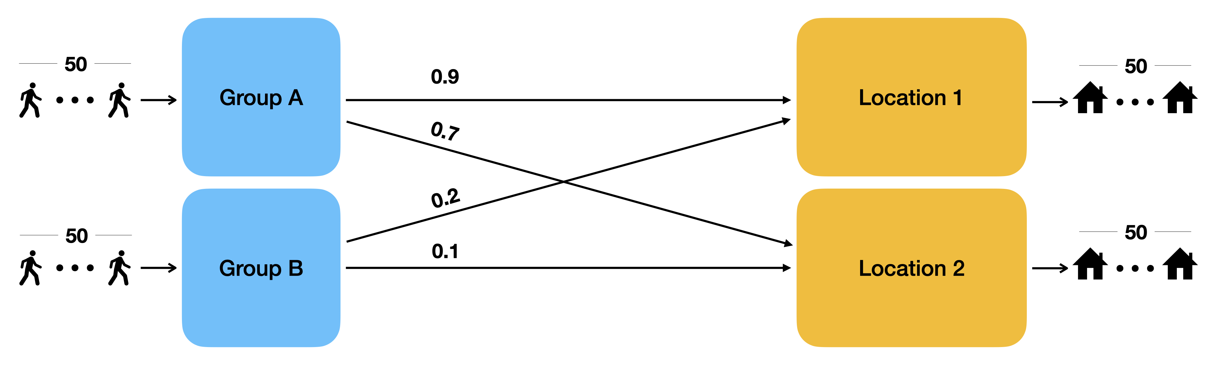
Figure 1: There are two groups $\{A,B\}$ with $50$ refugees each and two locations $\{1,2\}$ with capacities of $50$. Each case of Group A finds employment with probability $0.9$ when assigned to Location 1 and $0.7$ when assigned to Location 2. For cases of Group B the probabilities are $0.2$ and $0.1$.

Although these algorithms represent a significant leap in the use of analytics to drive societal impact, one may worry that global optimization may consistently disadvantage a particular subgroup of refugees, e.g., subgroups defined by country of origin, age, or educational background. For example, consider the setting of Figure 1, where members of groups A and B each achieve higher employment in Location 1. In this example, global optimization (i.e., optimizing for average employment across all cases) yields outcomes that are clearly unfair for any reasonable definition of group fairness, as all members of Group B are assigned to their least preferred location (Location 2) while all members of Group A are assigned to their most preferred location (Location 1).

Why might group fairness be of central importance in the setting of dynamic refugee assignment? First, the use of a refugee assignment algorithm can be jeopardized from a legal standpoint if it has disparate impacts on refugees from different origin countries (see Recital 71 of the EU GDPR [Vol22]). Second, fairness of employment outcomes across key subgroups has been identified by decision-makers as an important goal when designing algorithms. This sentiment is captured by Sjef van Grinsven, Director of Projects at COA:

“Because of the ever growing impact of AI on society, the topic of fairness is becoming increasingly important. For an organization such as COA, a semi-governmental organization working with a vulnerable target group, implementing fairness is not what you would call desirable: it’s an absolute necessity. The challenge is to translate an abstract concept like fairness into concrete programmable choices.”

Achieving the goal of incorporating group fairness into an algorithm for the dynamic refugee assignment problem is often not a straightforward task. First, there is a large and ever-growing number of ways that a policy maker may describe the fairness (or lack thereof) of an assignment of refugees to locations (see Section 1.2). Second, it is not clear how to extend fairness rules that are specified for static assignments to settings where refugees arrive and are assigned sequentially. To be practically useful to policy makers, any framework to measure group fairness in dynamic refugee resettlement must be flexible (seamlessly adapting to different fairness rules) and simple (not requiring the policy maker to reason about the intricacies of the dynamic arrivals of refugees); see discussion in Section 6.4.

1.1 Our contributions

In this paper, we introduce such a framework for incorporating group fairness into the dynamic refugee assignment problem (Section 2.2). Our framework does not require policy makers to define a notion of fairness that explicitly accounts for the stochastic arrival process of refugees. Instead, our framework only requires policy makers to specify an ex-post feasible fairness rule that, in turn, generates a minimum requirement on the average employment probability for each group. By only requiring the fairness rule to be defined when all refugee arrivals are known upfront, our framework is easy to understand by practitioners and thus desirable from an adoptability standpoint. At the same time, the minimum requirement can be generated using a variety of simple and interpretable definitions of group fairness from the literature, e.g., MaxMin, Randomized, Proportionally Optimized within group. All together, our framework provides policy makers with a concrete way to evaluate whether a particular deployed algorithm achieves the specified fairness criteria (Section 2.3); see further discussion regarding practical implications in Section 6.4.

Equipped with our framework for reasoning about group fairness in the dynamic refugee resettlement setting, we perform a numerical analysis of how well existing approaches fare with respect to different fairness criteria (Section 6.2). We analyze data from two partner organizations in the US and the Netherlands and show that a natural Bid Price Control (BP), similar to [AGP⁺21], can create frequent unfair group outcomes, when considering various fairness criteria considered in the literature. We also show that this is not simply a result of BP, but also occurs with a clairvoyant control that has advance knowledge of arrivals and assigns them optimally. Additionally, we show that a random assignment algorithm (a proxy for status quo procedures in the absence of optimization [BFH⁺18]) yields outcomes that are inefficient in terms of total employment and routinely fails to achieve group fairness according to the rules considered.

Motivated by the finding that existing approaches can lead to unfair assignments on real data, we develop two algorithms with provable guarantees that hold for any ex-post feasible fairness rule.

• First, we propose a modification of BP (Section 3) that includes dual variables for each group. These dual variables amplify employment probabilities at the group level to help direct the most valuable locations towards the groups that need them the most in order to meet their minimum requirements. We refer to this algorithm as Amplified Bid Price Control (ABP). ABP has strong performance guarantees at the population level (Theorem 1) when compared to an offline solution that meets the minimum requirement of every group. Moreover, in our data-driven numerical study, it incurs only a minimal loss ($\approx 0-1\%$) in total employment when compared to BP and the offline problem without fairness constraints (see Table 2 in Section 6.3). This suggests that, in practice, incorporating group fairness considerations need not be costly in terms of total employment. On the theoretical side, ABP also provides strong performance guarantees at the group level for groups with reasonably large sizes (Theorem 2), such as age or educational level (see Table 1 in Section 6). However, for groups with small sizes, such as many based on country of origin in the US, the algorithm has no meaningful performance guarantees and can exhibit unfair outcomes in numerical studies (Section 6.3).

• Our second algorithm, dubbed Conservative Bid Price Control (CBP), combines elements from ABP with reserve capacity at each location and occasional greedy decisions to overcome the poor performance of ABP with respect to small groups. Greedy steps sacrifice global efficiency to help boost the employment of groups that need it, and reserving capacity at each location helps ensure that regular assignments do not deplete the capacity of a location before a greedy decision can make use of it. With these changes, CBP has both population level performance guarantees (Theorem 3), and adds a guarantee that all groups, regardless of their size, will approximately meet their minimum requirements (Theorem 4). In our numerical results, we find that CBP incurs a small loss ($\approx 0-1\%$) in total employment when compared to ABP while approximately meeting the minimum requirements of all groups in all instances.

1.2 Related work

Refugee resettlement.

In the context of refugee resettlement, recent work introduces data analytics and market design to improve operational efficiency. Our work is closest to the aforementioned works [BFH⁺18, AAM⁺21, BP22, AGP⁺21] that optimize the assignment of refugees to locations, either in static or in dynamic settings, where the objective function is the average employment rate. [BP22, AGP⁺21] use resolving techniques, backtest on historical data, and find that their online algorithms incur little loss relative to the optimal objective in hindsight. [BP22] incorporates an additional queuing/load balancing component in their objective to ensure that the resources at each location are evenly utilized throughout the year. The methods proposed by [BP22, AGP⁺21] are currently being used in Switzerland and the US, respectively. [GP19] studies a variation wherein the employment score at a location is a submodular function of the assigned refugees. In terms of fairness, [AEM18] considers envy-freeness between locations. To the best of our knowledge, our work is the first to design algorithms that promote fairness for refugees. Closely connected to our motivation is [BM21], which identifies similar concerns to ours (Section 6.2) when studying a static refugee resettlement problem, but does so with a more restricted lens of group fairness and does not provide algorithmic solutions to overcome these concerns. Other works in refugee resettlement design mechanisms to satisfy preferences of refugees and locations [AE16, MR14, NNT21, JT18, ACGS18], or allow decision-makers to trade-off between refugees’ preferences and employment maximization [ABH22, DKT23, OS22].

Methodological connections to online packing.

Our formulation and algorithms are similar to those studied in online packing problems, including canonical quantity-based network revenue management [MVR99] and the AdWord problem [MSVV07]. These are sequential decision-making problems, in which a stream of $T$ requests occurs, and a decision is made for each request: for network revenue management the decision is to accept/reject, for AdWords it is where to accept a request. In both problems accepting a request yields a reward (in AdWords, the reward depends on where), but also consumes a set of resources. The objective is to maximize the accumulated rewards and is often measured by regret, defined by the difference in accumulated rewards compared to the offline optimal solution, while satisfying capacity constraints [TVRVR04]. Classical bid price control [Wil92] and randomized LP approaches [TVR99] have long been known to achieve the fluid optimal $O(\sqrt{T})$ regret [TVR98] for these problems, though these approaches have been improved through resolving techniques, that eventually led to $O(1)$ regret guarantees [RW08, JK12, BW20, VB21, VBG21, BF19]. All of these approaches require resolving some LP from time to time. In this paper’s context, which includes fairness constraints, using resolving can lead to infeasibility issues along the horizon (see Appendix B). Moreover, our methods, which do not resolve, yield results close to the hindsight-optimal solution on real-world data sets (Section 6). Thus, we do not focus on expanding resolving methods to this setting, and leave this as a future area of work.

An orthogonal set of approaches to online packing problems arises in online convex optimization [Haz16, AD15]. These approaches do not rely on resolving, but cannot easily adapt to the presence of sub-linear size groups, as we find in our work. Applying previous results, from either stream, leads to vacuous guarantees for small groups (see discussion after Theorem 2), forcing us to develop new algorithmic and analytical ideas to warrant good performance for all groups (Theorem 4).

Fairness considerations.

Beyond refugee resettlement, fairness has been studied in many other operational settings such as kidney exchange [BFT13], food banks [SJBY22], online advertising [FHK⁺10, BLM21, BCCM22], and pricing [CEL22]; see also [DAFST22] for a wider review of applications of algorithmic fairness in operations. We now expand on the connection to works that are closer to ours. The trade-off between optimizing a global objective and incorporating fairness considerations is often captured in the literature via the price of fairness [BFT11, BFT12]. Quantifying fairness considerations via a requirement for each group resembles a setting from the literature where one aims to minimize wait time in a queuing system subject to a requirement on the idle time of each server [AW10]. A major difference to these works is that our setting involves dynamic decisions occurring over a finite number of rounds; the uncertainty in arrivals introduces complexities, especially with respect to groups with small arrival probability. In contrast, the former line of works assumes a static optimization while the latter focuses on a steady-state behavior of the system.

The fairness rules that we consider in our work are closely related to two dynamic decision-making lines of work from the literature. The Proportionally Optimized fairness rule (Example 2) aims to mitigate the negative effect that the existence of a group may cause to members of another group by positing that the group should have performance at least as good as what it would have in isolation. This was initially studied in a stochastic online learning setting with disjoint groups [RSWW18] and has been subsequently extended in a non-stationary setting with overlapping groups [BL20]. A key difference of our application is that individual cases are organically coupled via resource constraints; as a result, it is not clear how to define in isolation. To incorporate this aspect, we extend the rule by asserting that the average employment probability of each group is no less than what it would have been if the group optimized its assignments over hypothetical capacities proportional to its size (without considering other groups). The Maxmin fairness rule (Example 3) aims to optimize the performance of the group with the lowest average employment outcome; this is a classical fairness criterion [KS75, Raw04, KRT99, AS07, BFT11]. In a dynamic setting, there has been a sequence of recent works studying how to optimize this quantity [LIS14, MNR22, MXX22, MXX21]. A key difference in our setting is that we aim to optimize the global objective subject to a requirement on the lowest group’s outcome, rather than maximizing the latter quantity only with no regard to global efficiency..

Finally, fairness has been widely studied in the context of supervised machine learning with multiple different definitions mostly aiming to equalize a fairness metric across different groups starting from [HPS16, Cho17, KMR17, CG18]. The challenge in that line of literature is statistical: how can one try to use an inaccurate machine learning model? In contrast, we assume that the machine learning model is completely accurate (with respect to employment probabilities) and the challenge arises from the uncertainty in the arrival process.

2 Model

In this section, we define the dynamic refugee assignment problem (Section 2.1), introduce a framework that incorporates group fairness (Section 2.2), and formalize our objectives (Section 2.3).

2.1 The Dynamic Refugee Assignment Problem

A refugee resettlement agency or decision maker (DM) is faced with the task of assigning $T$ refugee cases with labels $\{1,\ldots,T\}$ to a set $\mathcal{M}$ of resettlement locations in a host country; we denote by $M$ the number of locations. For simplicity, we assume that each refugee case consists of one individual. Each location $j\in\mathcal{M}$ has a capacity $s_{j}$, i.e., it can have at most $s_{j}$ cases assigned to it. We assume there is sufficient capacity such that $\sum_{j\in\mathcal{M}}s_{j}\geq T$. We denote by $\hat{s}_{j}=s_{j}/T$ the fraction of cases that can be assigned to each location $j$. We refer to $\hat{s}_{j}$ as the fractional capacity of location $j$ and denote the minimum fractional capacity by $\hat{s}_{\min}=\min_{j\in\mathcal{M}}\hat{s}_{j}$. The sequence of refugee cases is denoted by the stochastic process $\boldsymbol{\omega}\equiv(\boldsymbol{\theta}_{1},\ldots,\boldsymbol{\theta}_{T})$, where $\boldsymbol{\theta}_{t}\in\Theta$ denotes the random feature vector associated with refugee case $t$. The feature vectors $\boldsymbol{\theta}_{t}$ are drawn independently from known probability distributions $\mathcal{P}_{t}$ over $\Theta$ and they include information that is known about the refugee such as their country of origin, gender, education level, etc. We denote the set of all possible realizations of this stochastic process by $\Omega\equiv\Theta^{T}$.

The feature vector $\boldsymbol{\theta}_{t}$ lets us extract the following relevant information about refugee case $t$. First, we let $w_{t,j}\equiv w_{j}(\boldsymbol{\theta}_{t})\in[0,1]$ denote the estimated probability that a refugee with features $\boldsymbol{\theta}_{t}$ finds employment at each location $j\in\mathcal{M}$ within a specified time frame of interest. The function $\boldsymbol{w}:\Theta\to[0,1]^{M}$ is estimated by a supervised machine learning model and is available to the DM. We assume that for a case $t$, $\mathcal{P}_{t}$ is such that $\boldsymbol{w}$ is drawn from a continuous cumulative distribution function over $[0,1]^{M}$, and often refer to $w_{t,j}$ as the score of case $t$ at location $j$. Second, we let $g(t)\equiv g(\boldsymbol{\theta}_{t})\in\mathcal{G}$ denote the (unique) group of case $t$, where the set of all groups $\mathcal{G}$ has cardinality $G$. Group definitions are outside the purview of the DM and are decided by an external policy maker; for example, groups may be defined by level of education or country of origin.

We now specify our assumptions regarding the non-stationarity of the arrival process $\mathcal{P}_{t}$. Letting $p_{g}(t)$ be the probability that a case from group $g\in\mathcal{G}$ arrives in period $t$, we define the average arrival probability of group $g$ across the time horizon as $\bar{p}_{g}\triangleq\frac{1}{T}\sum_{t\in[T]}p_{g}(t),$ and the non-stationarity parameter $U=\min\{u\geq 1\colon p_{g}(t)/\bar{p}_{g}\in[1/u,u],~{}\forall g\in\mathcal{G},t\in[T]\}$. Although we allow $p_{g}(t)$ to evolve over time, we assume that the score $w_{t,j}$ is drawn identically across time condition on a group. This is formalized in the following assumption which we posit throughout the paper.

Assumption 1.

For $g\in\mathcal{G},t,t^{\prime}\in[T]$, condition on $g(t)=g(t^{\prime})=g$, $(w_{t,j})_{j\in\mathcal{M}}\stackrel{{\scriptstyle d}}{{=}}(w_{t^{\prime},j})_{j\in\mathcal{M}}$.

Refugee cases arrive in ascending order of their labels and, at each period $t=1,\ldots,T$, the DM observes the feature vector $\boldsymbol{\theta}_{t}$ associated with refugee case $t$ and needs to decide a location for the case. This decision needs to be non-anticipative and irrevocable: the DM needs to commit on the location for refugee case $t$ prior to seeing the information of cases $t^{\prime}>t$. Formally, we denote the DM’s decision for refugee case $t$ by the assignment vector $\mathbf{z}_{t}\equiv\mathbf{z}_{t}(\boldsymbol{\theta}_{1},\ldots,\boldsymbol{\theta}_{t})\in\{0,1\}^{M}$, where $\boldsymbol{\theta}_{1},\ldots,\boldsymbol{\theta}_{t}$ is the information that has been revealed to the DM after the arrival of case $t$, and where the equality $z_{t,j}=1$ holds if and only if refugee case $t$ is assigned to location $j\in\mathcal{M}$. We say that a sequence of assignments is feasible if and only if each case is assigned to a single location in a way that does not violate any location’s capacity; that is, a sequence of assignments ${\mathbf{z}}_{1},\ldots,{\mathbf{z}}_{T}\in\{0,1\}^{M}$ is feasible if $(\mathbf{z}_{1},\ldots,\mathbf{z}_{T})$ is an element of the fractional assignment polytope formally defined as

$$\tilde{\mathcal{Z}}=\left\{(\tilde{\mathbf{z}}_{1},\ldots,\tilde{\mathbf{z}}_{T})\in\mathbb{R}_{\geq 0}^{T\times M}:\quad\begin{aligned} \sum_{j\in\mathcal{M}}\tilde{\mathbf{z}}_{t,j}=1&&\forall t\in\{1,\ldots,T\}&&\textrm{and}&&\sum_{t=1}^{T}\tilde{\mathbf{z}}_{t,j}\leq s_{j}&&\forall j\in\mathcal{M}.\end{aligned}\right\}$$

We denote the restriction of $\tilde{\mathcal{Z}}$ to the integers by $\mathcal{Z}=\tilde{\mathcal{Z}}\cap\{0,1\}^{T\times M}$.

In the absence of group fairness considerations, the DM aims to select a feasible sequence of integer assignments that achieves high average employment probability across refugee cases. Formally, a sequence of assignments ${\mathbf{z}}_{1},\ldots,{\mathbf{z}}_{T}\in\mathcal{Z}$ induces a global objective value of $\frac{1}{T}\sum_{t=1}^{T}\sum_{j\in\mathcal{M}}w_{t,j}z_{t,j}$, where we recall that $w_{t,j}$ and $z_{t,j}$ are shorthand for $w_{j}(\boldsymbol{\theta}_{t})$ and $z_{t,j}(\boldsymbol{\theta}_{1},\ldots,\boldsymbol{\theta}_{t})$. To incorporate group objectives, we denote the set of cases that belong to group $g$, among the first $t$ arrivals of realization $\boldsymbol{\omega}$, by $\mathcal{A}(g,t)\equiv\mathcal{A}(g,t,\boldsymbol{\omega})\triangleq\left\{\tau\leq t:g(\boldsymbol{\theta}_{\tau})=g\right\}$ and the cardinality of this set by $N(g,t)\equiv N(g,t,\boldsymbol{\omega})\triangleq|\mathcal{A}(g,t,\boldsymbol{\omega})|$. A group is called non-empty for realization $\boldsymbol{\omega}$ if $N(g,T,\boldsymbol{\omega})>0$. This lets us define, for each group $g\in\mathcal{G}$, the average employment probability of that group as

$$\alpha_{g}(\boldsymbol{\omega})\triangleq\frac{1}{N(g,T,\boldsymbol{\omega})\lor 1}\sum_{t\in\mathcal{A}(g,T)}\sum_{j\in\mathcal{M}}w_{t,j}z_{t,j}.$$

2.2 Our Framework for Group Fairness

Our goal is not to impose a definition of group fairness; rather, it is to provide flexible and expansive frameworks that allow policy makers to specify the group fairness desiderata they wish to attain. With this in mind, our framework allows external policy makers to specify a minimum requirement for every group and every realization of the dynamic refugee assignment problem. Formally, the policy maker selects a fairness rule $\mathcal{F}$ which provides a mapping $O_{g,\mathcal{F}}:\Omega\to[0,1]$ for each group $g\in\mathcal{G}$, where the quantity $O_{g,\mathcal{F}}(\boldsymbol{\omega})$ represents the minimum requirement on the average employment score of members of group $g$. Of course, not all requirements are achievable even when one is granted the benefit of hindsight. Hence, our framework necessitates that the provided requirements satisfy a notion of ex-post feasibility for a fractional version of the assignment problem.

Definition 1.

A fairness rule $\mathcal{F}$ is ex-post feasible if, for every sample path $\boldsymbol{\omega}\in\Omega$, there exist fractional ex-post decisions $\tilde{z}_{t,j}(\boldsymbol{\omega})\in[0,1]$ for each case $t\in[T]$ and location $j\in\mathcal{M}$ such that

$$\begin{aligned} (\tilde{\textbf{z}}_{1},\ldots,\tilde{\textbf{z}}_{T})\in\tilde{Z}&&\text{and}&&\frac{1}{N(g,T)\lor 1}\sum_{t\in\mathcal{A}(g,T)}\sum_{j\in\mathcal{M}}w_{t,j}\tilde{z}_{t,j}&\geq O_{g,\mathcal{F}}(\boldsymbol{\omega})&&\forall g\in\mathcal{G}.\end{aligned}$$

Note that the constraints imply $O_{g,\mathcal{F}}(\boldsymbol{\omega})=0$ for an empty group $g$, which we assume throughout.

As long as the specified fairness rule $\mathcal{F}$ satisfies ex-post feasibility, our algorithms will achieve favorable group performance guarantees despite not having the benefit of hindsight; see Sections 3 and 4. Of course, for this group fairness framework to be meaningful, it needs to capture existing fairness notions as special cases. To demonstrate the versatility of our framework, we provide three examples of ex-post feasible fairness rules. We note that for the first two examples to fulfill ex-post feasibility, it is necessary that Definition 1 allows for fractional assignments $\tilde{\mathbf{z}}$.

Example 1 (Random Fairness Rule).

In many host countries, the status quo of refugee resettlement assignments is effectively random [BFH⁺18]. The random fairness rule protects groups from being worse off than this status quo benchmark, thus fulfilling the maxim of “primum non nocere” (“do no harm”). To mimic a random assignment, for each realization $\boldsymbol{\omega}\in\Omega$ and non-empty group $g\in\mathcal{G}$, we consider the fractional assignment $\tilde{z}_{t,j}^{\mathrm{random}}=\frac{s_{j}}{\sum_{j^{\prime}\in\mathcal{M}}s_{j^{\prime}}}$ and set the minimum requirement as

$$O_{g,\mathrm{random}}(\boldsymbol{\omega})=\frac{1}{N(g,T)}\sum_{t\in\mathcal{A}(g,T)}\sum_{j\in\mathcal{M}}w_{t,j}\tilde{z}_{t,j}^{\mathrm{random}}.$$

Example 2 (Proportionally Optimized Fairness Rule).

The random fairness rule fulfills “primum non nocere” but does not use synergies between different arrivals of one group. The proportionally optimized fairness rule posits that, for every realization $\boldsymbol{\omega}\in\Omega$, a non-empty group $g\in\mathcal{G}$ receives a capacity $s_{j,g}=N(g,T)\hat{s}_{j}$, proportional to the group size, for all locations $j\in\mathcal{M}$. It then optimizes their assignment over the fractional assignment polytope restricted to group $g$, i.e., $\mathcal{\tilde{Z}}_{g}=\{\boldsymbol{\tilde{z}}\in[0,1]^{\mathcal{A}(g,T)\times M}\colon\sum_{j\in\mathcal{M}}\tilde{z}_{t,j}\leq 1,\forall t\in\mathcal{A}(g,T);~{}\sum_{t\in\mathcal{A}(g,T)}\tilde{z}_{t,j}\leq s_{j,g},\forall j\in\mathcal{M}\}.$ The resulting minimum requirement captures the maximum value a group would receive in isolation:

$$O_{g,\mathrm{pro}}(\boldsymbol{\omega})=\max_{\boldsymbol{\tilde{z}}\in\mathcal{\tilde{Z}}_{g}}\frac{1}{N(g,T)}\sum_{t\in\mathcal{A}(g,T)}\sum_{j\in\mathcal{M}}w_{t,j}\tilde{z}_{t,j}.$$

This reflects the principle that a group should not be worse off due to the presence of other groups, which has been studied in sequential group fairness without resource constraints (see Section 1.2).

Example 3 (MaxMin Fairness Rule).

As neither of the above examples guarantees a high minimum requirement for the most vulnerable (least employable) group, the well-studied MaxMin fairness rule is a natural alternative. The corresponding minimum requirement for realization $\omega\in\Omega$ is the same across all non-empty groups $g\in\mathcal{G}$ and maximizes the minimum average value across all groups:

$$O_{g,\mathrm{maxmin}}(\boldsymbol{\omega})=\max_{\boldsymbol{z}\in\tilde{\mathcal{Z}}}\min_{g^{\prime}\in\mathcal{G}\colon N(g^{\prime},T)>0}\frac{1}{N(g^{\prime},T)}\sum_{t\in\mathcal{A}(g^{\prime},T)}\sum_{j\in\mathcal{M}}w_{t,j}z_{t,j}.$$

Note that, although fairness rules are formally defined as a mapping from all possible realizations to minimum requirements, the examples above illustrate that fairness rules can be succinctly specified in an interpretable way.

Our work assumes that a policy maker has provided minimum requirements corresponding to an ex-post feasible fairness rule and we often drop the notational dependence on $\mathcal{F}$. In Section 6 we investigate the differences between the three rules we presented here. Finally, some of our results require the fairness rule $\mathcal{F}$ to satisfy a lower bound on a notion of slackness, defined as $\varepsilon_{g,\mathcal{F}}=\mathbb{E}_{\boldsymbol{\theta}}\left[\max_{j\in\mathcal{M}}w_{j}(\boldsymbol{\theta})\,\middle|\,g(\boldsymbol{\theta})=g\right]-\mathbb{E}_{\boldsymbol{\omega}}[O_{g,\mathcal{F}}(\boldsymbol{\omega})]$, which is the expected difference between the maximum score conditional on a group $g$ and its corresponding requirement. This quantity is non-negative by ex-post feasibility and captures the difficulty to achieve the minimum requirements.

Definition 2.

A fairness rule $\mathcal{F}$ has slackness $\varepsilon$ if $\varepsilon_{g,\mathcal{F}}\geq\varepsilon>0$ for every group $g$.

Note that the only rule giving $\varepsilon_{g,\mathcal{F}}=0$ must assign every case of group $g$ to the location maximizing the employment score. In that sense, it is natural to assume that $\varepsilon_{g,\mathcal{F}}$ be greater than $0$, though some of our results require it to be bounded away from $0$.

2.3 Objectives for our Setting

The minimum requirements serve as an algorithmic benchmark: for a realization $\boldsymbol{\omega}\in\Omega$, we want an algorithm to achieve average employment probability for every group that is lower bounded by $O_{g,\mathcal{F}}(\boldsymbol{\omega})$. This gives the definition of ex-post $g-$regret: for a realization $\omega\in\Omega$, if an algorithm induces average employment probability $\alpha_{g}(\boldsymbol{\omega})$ for a group $g\in\mathcal{G}$, then its ex-post $g$-regret is

$$\mathcal{R}^{\mathrm{ex}}_{g,\mathcal{F}}(\boldsymbol{\omega})=O_{g,\mathcal{F}}(\boldsymbol{\omega})-\alpha_{g}(\boldsymbol{\omega}).$$

Though our algorithms have strong guarantees on ex-post-$g$-regret for fairness rules that fulfill a certain “sensitivity” condition (see Section 5), such guarantees are not possible for arbitrary fairness rules (see end of this section), which we focus on for most of the paper. For these we consider the following weaker benchmark that consists of the minimum of $O_{g,\mathcal{F}}(\boldsymbol{\omega})$ and its expectation over $\boldsymbol{\omega}^{\prime}\sim\mathcal{P}_{1}\times\cdots\times\mathcal{P}_{T}$. Formally, the $g$-regret of a group $g\in\mathcal{G}$ is defined by

$$\mathcal{R}_{g,\mathcal{F}}(\boldsymbol{\omega})\triangleq\min\left\{O_{g,\mathcal{F}}(\boldsymbol{\omega}),\mathbb{E}_{\boldsymbol{\omega}^{\prime}}[O_{g,\mathcal{F}}(\boldsymbol{\omega}^{\prime})]\right\}-\alpha_{g}(\boldsymbol{\omega}).$$

We now focus on our global objective, i.e., to maximize the average employment probability for all refugee cases independent of group, subject to the group-level minimum requirements. To evaluate how well an algorithm performs, we compare against the best sequence of fractional assignments for the realization $\boldsymbol{\omega}$. We note that, as before, we need to use fractional assignments to allow for general ex-post feasible fairness rules. Formally,

$$O^{\star}_{\mathcal{F}}(\boldsymbol{\omega})\triangleq\quad \underset{\mathbf{\tilde{z}}\in\tilde{\mathcal{Z}}}{\textnormal{max}}\frac{1}{T}\sum_{t=1}^{T}\sum_{j\in\mathcal{M}}w_{t,j}\tilde{z}_{t,j}\textnormal{ s.t. }\forall g:\sum_{t\in\mathcal{A}(g,T)}\sum_{j\in\mathcal{M}}w_{t,j}\tilde{z}_{t,j}\geq N(g,T)\;O_{g,\mathcal{F}}(\boldsymbol{\omega}). \text{OFFLINE}_{\mathcal{F}}$$ ()

An algorithm aims to make sequential irrevocable integral decisions $z_{t}\in\{0,1\}^{\mathcal{M}}$ that minimize, with high probability, the global regret

$$\mathcal{R}_{\mathcal{F}}(\boldsymbol{\omega})\triangleq\mathbb{E}_{\boldsymbol{\omega}^{\prime}}[O_{\mathcal{F}}^{\star}(\boldsymbol{\omega}^{\prime})]-\frac{1}{T}\sum_{t=1}^{T}\sum_{j\in\mathcal{M}}w_{t,j}z_{t,j},$$

while also achieving favorable $g$-regret guarantees for all groups $g\in\mathcal{G}$. In particular, we say that an algorithm has favorable regret guarantees if $\mathcal{R}_{\mathcal{F}}(\boldsymbol{\omega})$ and $\mathcal{R}_{g,\mathcal{F}}(\boldsymbol{\omega})$ (or $\mathcal{R}^{\mathrm{ex}}_{g,\mathcal{F}}(\boldsymbol{\omega})$ in the case of “sensitive” fairness rules) are upper bounded by a quantity that vanishes to zero as the number of cases $T$ tends to infinity with high probability, for all groups $g\in\mathcal{G}$.

We now briefly motivate our choice of benchmarks by describing several impossibility results.

• Meaningful bounds for arbitrary fairness rules require us to weaken the ex-post requirement: there exist ex-post feasible fairness rules (Appendix C.1) that do not admit high-probability vanishing ex-post $g$-regret or a high multiplicative analogue thereof, $\alpha_{g}(\boldsymbol{\omega})/O_{g,\mathcal{F}}(\boldsymbol{\omega})$.

• This cannot be fixed by using the expected minimum requirement $\mathbb{E}_{\boldsymbol{\omega}^{\prime}}[O_{g,\mathcal{F}}(\boldsymbol{\omega}^{\prime})]$ as a benchmark: there exist ex-post feasible fairness rules (Appendix C.2) that do not admit constant multiplicative approximation of $\mathbb{E}_{\boldsymbol{\omega}^{\prime}}[O_{g,\mathcal{F}}(\boldsymbol{\omega}^{\prime})]$ with high probability. Together with the previous point, this motivates $g$-regret as our benchmark.

• Meaningful ex-post bounds are also unattainable for global regret: we construct (Appendix C.3) an ex-post feasible fairness rule such that no algorithm can achieve both vanishing $g$-regret and an average employment probability with vanishing difference to the sample-path optimum $O^{\star}(\boldsymbol{\omega})$. This motivates us to use the the expected optimum $\mathbb{E}_{\boldsymbol{\omega}^{\prime}}\left[O^{\star}(\boldsymbol{\omega}^{\prime})\right]$ as a benchmark.

• Although the above results rely on unusual fairness rules, we also show (Appendix C.4) that even for the MaxMin fairness rule (Example 3), no algorithm can obtain, with high probability, both vanishing ex-post $g$-regret and vanishing global regret.

Finally, for our regret to be well-defined, we require measurability of $O_{\mathcal{F}}^{\star}$ and $O_{g,\mathcal{F}}$ for every group $g\in\mathcal{G}$. We show in Appendix C.5 that all fairness rules described in Section 2.2 satisfy this.

3 Amplified Bid Price Control

Our approach builds on the classical Bid Price Control that minimizes global regret (without fairness considerations) and was initially developed in the context of network revenue management [TVR98], which is an admission control problem with only accept/reject decisions. We show that a simple modification of this algorithm yields global regret that vanishes in $T$ at a rate of $1/\sqrt{T}$ and $g$-regret that scales as $1/\sqrt{\bar{p}_{g}\cdot T}$. In the next section, we extend our algorithm to attain $g$-regret that scales as $1/\sqrt{T}$.

Bid Price Control or BP as a shorthand aims to maximize the global objective subject to capacity constraints, i.e., find an assignment $\boldsymbol{z}\in\mathcal{Z}$ that maximizes $\sum_{t=1}^{T}\sum_{j\in\mathcal{M}}w_{t,j}z_{t,j}$. Myopically assigning each case to the location that maximizes its score may seem like a natural candidate algorithm to achieve this objective; yet, this quickly depletes the capacities at locations with universally good refugee employment prospects. As a result, optimally assigning a case needs to take into account not only the present case-location score but also the opportunity cost of a slot at location $j$, i.e., the potential decrease in future assignment scores due to depleted capacity at $j$. Bid Price Control quantifies the opportunity cost of each assignment and additively adjusts the employment probabilities by this amount. Effectively, this penalizes the selection of locations that are valuable in the future. That said, this adjustment of scores does not take into account group-fairness concerns and may severely violate minimum requirements (see Figure 4 of Section 6).

Our modification (Algorithm 1), which we term Amplified Bid Price Control or ABP as a shorthand, explicitly captures these fairness concerns by introducing group-dependent score amplifiers. In particular, the scores of each case are first scaled by their group’s amplifier and are then additively adjusted by the opportunity cost of each potential assignment. These amplifiers help direct resources towards groups that need them the most in order to satisfy their minimum requirements. For example, a group that is likely to have a loose fairness constraint in $\text{OFFLINE}_{\mathcal{F}}$ would have a small amplifier and be assigned based on the tradeoff between $w_{t,j}$ and the locations’ opportunity cost. To formalize the above intuition, we denote by $\mu^{\star}_{j}$ and $\lambda^{\star}_{g}$ the opportunity cost of location $j\in\mathcal{M}$ and the amplifier of group $g\in\mathcal{G}$, respectively. These quantities are initially instantiated (see line 1 in Algorithm 1); we elaborate on this instantiation below. ABP wants to assign case $t$ to the location

$$J^{\mathrm{WAB}}(t)\triangleq\arg\max_{j\in\mathcal{M}}(1+\lambda_{g(t)}^{\star})w_{t,j}-\mu_{j}^{\star},$$

breaking ties in favor of the smallest index. That said, if this location has no capacity, the final assignment $J^{\mathrm{ABP}}(t)$ is a location with the most remaining capacity.

input : Capacity $s_{j}$ for $j\in\mathcal{M}$; Time horizon $T$; Fairness rule $\mathcal{F}$ inducing scores $O_{g}(\omega)$

1 Set $(\boldsymbol{\mu}^{\star},\boldsymbol{\lambda}^{\star})\leftarrow\arg\min_{\boldsymbol{\mu}\in\mathbb{R}_{+}^{M},\boldsymbol{\lambda}\in\mathbb{R}_{+}^{G}}\mathbb{E}\left[L(\boldsymbol{\mu},\boldsymbol{\lambda})\right]$ where $L(\boldsymbol{\mu},\boldsymbol{\lambda})$ is defined in (LAGR)

2 for case $t=1,\ldots,T$ of group $g(t)\in\mathcal{G}$ with scores $w_{t,j}$ for $j\in\mathcal{M}$ do

3       $J^{\mathrm{ABP}}(t)\leftarrow J^{\mathrm{WAB}}(t)$ where $J^{\mathrm{WAB}}(t)\leftarrow\arg\max_{j\in\mathcal{M}}(1+\lambda_{g(t)}^{\star})w_{t,j}-\mu_{j}^{\star}$

4       if $J^{\mathrm{WAB}}(t)$ has no capacity then  $J^{\mathrm{ABP}}(t)\leftarrow$ a location with most remaining capacity

5      

Algorithm 1 Amplified Bid Price Control

We now expand on the instantiation of $\boldsymbol{\mu}^{\star},\boldsymbol{\lambda}^{\star}$. The problem without fairness constraints aims to find an assignment ${\boldsymbol{z}}\in{\mathcal{Z}}$ that maximizes $\sum_{t\in[T]}\sum_{j\in\mathcal{M}}w_{t,j}z_{t,j}$. The classical Bid Price Control computes opportunity costs $\boldsymbol{\mu}^{\star}$ by solving its Lagrangian relaxation over the fractional assignments without capacity constraints, i.e., the polytope $\widehat{\mathcal{Z}}\triangleq\{\widehat{\boldsymbol{z}}\in[0,1]^{T\times M}\colon\sum_{j\in\mathcal{M}}\widehat{z}_{t,j}=1\forall t\}$:

$$L(\boldsymbol{\mu})=\frac{1}{T}\max_{\widehat{\boldsymbol{z}}\in\widehat{\mathcal{Z}}}\left(\sum_{t=1}^{T}\sum_{j\in\mathcal{M}}w_{t,j}\widehat{z}_{t,j}+\sum_{j\in\mathcal{M}}\mu_{j}\left(s_{j}-\sum_{t\in[T]}\widehat{z}_{t,j}\right)\right),$$

where $\mu_{j}\geq 0$ is the Lagrange multiplier associated with the capacity constraint for location $j$. For any vector $\boldsymbol{\mu}\geq 0$, $L(\boldsymbol{\mu})$ upper bounds the original objective. BP selects Lagrange multipliers $\boldsymbol{\mu}^{\star}\in\arg\min_{\boldsymbol{\mu}\in\mathbb{R}_{+}^{M}}\mathbb{E}\left[L(\boldsymbol{\mu})\right]$ that give the tightest upper bound in expectation. For each case $t$, the optimal $\widehat{\boldsymbol{z}}$ in the inner maximization of $L(\boldsymbol{\mu}^{\star})$ chooses the location $j$ that maximizes $w_{t,j}-\mu^{\star}_{j}$. This matches the intuition that the multiplier $\mu^{\star}_{j}$ is the opportunity cost associated with location $j$.

We follow a similar approach while also incorporating group fairness constraints. In particular, denoting the Lagrange multiplier associated with the constraint for group $g$ by $\lambda_{g}$, the Lagrangian relaxation $L(\boldsymbol{\mu},\boldsymbol{\lambda})$ of our offline maximization program ($\text{OFFLINE}_{\mathcal{F}}$) is written as:

$$\max_{\widehat{\boldsymbol{z}}\in\widehat{\mathcal{Z}}}\frac{1}{T}\left(\sum_{t=1}^{T}\sum_{j\in\mathcal{M}}w_{t,j}\widehat{z}_{t,j}+\sum_{j\in\mathcal{M}}\mu_{j}\left(s_{j}-\sum_{t=1}^{T}\widehat{z}_{t,j}\right)+\sum_{g\in\mathcal{G}}\lambda_{g}\left(\sum_{t\in\mathcal{A}(g,T)}\sum_{j\in\mathcal{M}}w_{t,j}\widehat{z}_{t,j}-O_{g}N(g,T)\right)\right).$$

Rearranging terms, we find that $\widehat{z}_{t,j}$ appears as a coefficient for $(w_{t,j}-\mu_{j}+\lambda_{g(t)}w_{t,j})=(1+\lambda_{g(t)})w_{t,j}-\mu_{j}$. Similar to BP, the maximizing assignment $\widehat{\boldsymbol{z}}\in\widehat{\mathcal{Z}}$ now sets, for each case $t$, $\widehat{z}_{t,j}=1$ for the location $j$ that maximizes $(1+\lambda_{g(t)})w_{t,j}-\mu_{j}$. Hence, the Lagrangian relaxation is

$$L(\boldsymbol{\mu},\boldsymbol{\lambda})=\frac{1}{T}\left(\sum_{t=1}^{T}\max_{j\in\mathcal{M}}((1+\lambda_{g(t)})w_{t,j}-\mu_{j})+\sum_{j\in\mathcal{M}}\mu_{j}s_{j}-\sum_{g\in\mathcal{G}}\lambda_{g}O_{g}N(g,T)\right).$$ (LAGR)

ABP picks opportunity costs $\boldsymbol{\mu}^{\star}$ and amplifiers $\boldsymbol{\lambda}^{\star}$ that minimize $\mathbb{E}_{\boldsymbol{\omega}}[L(\boldsymbol{\mu},\boldsymbol{\lambda})]$ subject to non-negativity. As alluded to above, the scores of an arrival are amplified by $\lambda_{g}$ before they are additively adjusted by opportunity cost $\mu_{j}$. Further, by the same reasoning as for BP, $L(\boldsymbol{\mu},\boldsymbol{\lambda})\geq O^{\star}$ for any $\boldsymbol{\mu},\boldsymbol{\lambda}\geq 0$. In particular, $L(\boldsymbol{\mu}^{\star},\boldsymbol{\lambda}^{\star})\geq O^{\star}$ and thus $\mathbb{E}_{\boldsymbol{\omega}}[L(\boldsymbol{\mu}^{\star},\boldsymbol{\lambda}^{\star})]$ is an upper bound for $\mathbb{E}_{\boldsymbol{\omega}}[O^{\star}]$. With $\mathbb{E}_{\boldsymbol{\omega}}[L(\boldsymbol{\mu},\boldsymbol{\lambda})]$ being an expectation over convex functions (the maximum across linear functions), it is a convex function of $\boldsymbol{\mu},\boldsymbol{\lambda}$ enabling the efficient instantiation of $\boldsymbol{\mu}^{\star},\boldsymbol{\lambda}^{\star}$ (line 1 of Algorithm 1).

In the following theorems, we establish global and $g$-regret guarantees for ABP.

Theorem 1.

Fix an ex-post feasible fairness rule $\mathcal{F}$. For any $\delta>0$, Amplified Bid Price Control has global regret $\mathcal{R}_{\mathcal{F}}^{\mathrm{ABP}}\leq\sqrt{\frac{\ln(M/\delta)}{T}}\cdot\left(\frac{U}{\hat{s}_{\min}}+1\right)$ with probability at least $1-\delta$.

Theorem 2.

Fix an ex-post feasible fairness rule $\mathcal{F}$. For any $\delta>0$ and $g\in\mathcal{G}$, Amplified Bid Price Control has $g$-regret $\mathcal{R}_{g,\mathcal{F}}^{\mathrm{ABP}}\leq\sqrt{\frac{\ln(M/\delta)}{T}}\cdot\left(\frac{U^{2}}{\hat{s}_{\min}}+\sqrt{\frac{200}{\bar{p}_{g}}}\right)$ with probability at least $1-\delta$.

We make two observations about the practicality of these bounds. First, the capacity of each location typically scales with the number of cases $T$; which means that $\hat{s}_{\min}$ can be treated as a constant with respect to $T$. Therefore, the upper bound on global regret in Theorem 1 vanishes at a rate of $\tilde{O}(1/\sqrt{T})$ as $T$ grows large with high probability, e.g., when setting $\delta=1/T$. Second, the upper bound on $g$-regret in Theorem 2 vanishes when a group’s expected number of arrivals, $\bar{p}_{g}\cdot T$, is large (e.g., groups defined by age or education level; see Table 1). Specifically, the bound converges to zero at a rate of $\tilde{O}(1/\sqrt{T})$ when $\bar{p}_{g}$ is independent of $T$, i.e., when the expected size of group $g$ is linear in $T$. We show in Appendix D.1 that this convergence rate of $\tilde{O}(1/\sqrt{T})$ is unimprovable for both global regret and $g-$regret and thus Amplified Bid Price Control obtains near-optimal global efficiency and is group-fair for groups whose size increases linearly with $T$. That said, this scaling property may not hold for all groups, especially very small groups; the $g-$regret bound (Theorem 2) may thus be vacuous. In Section 4 we design an algorithm to address this problem.

Our starting point towards proving the theorems is to analyze the global and group objectives when case $t$ is always assigned to location $J^{\mathrm{WAB}}(t)$ irrespective of capacities. The objectives resulting from such an assignment have strong guarantees as we show in Lemma 3.1 and 3.2 using KKT conditions on $\boldsymbol{\mu}^{\star},\boldsymbol{\lambda}^{\star}$ and concentration arguments (see Appendix D.4 for full proofs).

Lemma 3.1.

We have $\sum_{t\in[T]}\mathbb{E}\left[w_{t,J^{\mathrm{WAB}}(t)}\right]\geq T\mathbb{E}\left[O^{\star}\right]$.

Lemma 3.2.

For any $t$ and $g$: $\mathbb{E}\left[w_{t,J^{\mathrm{WAB}}(t)}\,\middle|\,g(t)=g\right]\geq\mathbb{E}\left[O_{g}\right]-\sqrt{\frac{1}{\bar{p}_{g}T}}$.

Of course, ignoring capacities is unlikely to yield a feasible solution since we have hard capacity constraints. However, until some location runs out of capacity, ABP follows exactly these assignments. As a result, we want to bound the first time when a location’s capacity is depleted; we denote this time by $T_{\mathrm{emp}}$. The following lemma shows that, with high probability, this event occurs in the last $\Delta^{\mathrm{WAB}}:=\frac{U\sqrt{\frac{1}{2}T\ln\left(\frac{M+2}{\delta}\right)}}{\hat{s}_{\min}}$ periods. When $U=1$, i.e., when arrivals are i.i.d., the proof uses that, in expectation, $J^{\mathrm{WAB}}$ assigns at most $s_{j}$ cases to each location $j$. Hence, by concentration arguments, ABP uses at most $\hat{s}_{j}t+O(\sqrt{t\ln(\nicefrac{{1}}{{\delta}})})$ capacity in a location $j$ up to case $t$, and the algorithm does not deplete capacity in any location until assigning about $T-O(\sqrt{T\ln(\nicefrac{{1}}{{\delta}})})$ cases (see Appendix D.5 for a full proof).

Lemma 3.3.

For any $\delta>0$ with probability at least $1-\frac{M\delta}{M+2}$: $T_{\mathrm{emp}}\geq T-\Delta^{\mathrm{WAB}}$.

The proofs of Theorems 1 and 2 follow from combining Lemma 3.3 with Lemmas 3.1 and 3.2 respectively and are provided in Appendix D.2 and D.3.

4 Conservative Bid Price Control

The poor performance in Theorem 2 of ABP for small groups (i.e., groups whose total arrival number does not scale linearly in $T$) occurs due to two issues. First, ABP is designed to guarantee that the expected score of an arrival of a group is no less than the minimum requirement of that group. Roughly speaking, by central limit theorem, the average employment probability of a group concentrates near the expected score of one arrival of that group. That said, the rate at which this concentration occurs is inversely dependent on the size of the group. Second, consider an arrival $t$ after $T_{\mathrm{emp}}$, and suppose all the capacity at location $J^{\mathrm{WAB}}(t)$ is depleted. The expected score of this arrival may be below the group’s minimum requirement. For a group with few arrivals, this may have a significant effect on the group’s average score.

Our second algorithm (Algorithm 2), termed Conservative Bid Price Control, or CBP for short, is designed to address both of these issues by modifying ABP in two ways. First, CBP proactively offers high-score assignments to groups which are predicted to not meet their requirement otherwise. Second, CBP reserves capacity at locations so that late arrivals can still have favorable assignments. With these modifications, CBP approximately maintains the global guarantee of ABP while also obtaining strong guarantees for all groups (Theorem 4).

We first explain an intuition for how CBP predicts whether an arrival should receive a high-score assignment. Suppose for a group $g$ a clairvoyant knew its future arrivals and could assign each arrival greedily to the score-maximizing location. If assigning $t$ to $J^{\mathrm{WAB}}(t)$ and all subsequent arrivals of group $g(t)$ greedily is insufficient for $g(t)$ to meet its requirement, then our clairvoyant would assign arrival $t$ to the greedy location, denoted by $J^{\mathrm{GR}}(t)$. In contrast, if it is sufficient, our clairvoyant would assign arrival $t$ to $J^{\mathrm{WAB}}(t)$. To formalize this intuition, let $J^{\mathrm{CBP}}(\tau)$ denote the assignment that CBP made at time $\tau$. Then, our clairvoyant condition is

$$\sum_{\tau\in\mathcal{A}(g,t-1)}w_{\tau,J^{\mathrm{CBP}}(\tau)}+w_{t,J^{\mathrm{WAB}}(t)}+\sum_{\tau\in\mathcal{A}(g,T)\setminus\mathcal{A}(g,t)}w_{\tau,J^{\mathrm{GR}}(\tau)}\geq N(g,T)O_{g}(\boldsymbol{\omega}).$$

The terms on the left-hand side denote (i) the scores of already-assigned arrivals, (ii) the score of the current arrival $t$ under $J^{\mathrm{WAB}}$, and (iii) the cumulative scores of assigning the remaining arrivals of group $g$ greedily. Since there are exactly $N(g,T)$ summands on the left, this can be rewritten as

$$\sum_{\tau\in\mathcal{A}(g,t-1)}\left(w_{\tau,J^{\mathrm{CBP}}(\tau)}-O_{g}(\boldsymbol{\omega})\right)+w_{t,J^{\mathrm{WAB}}(t)}-O_{g}(\boldsymbol{\omega})+\sum_{\tau\in\mathcal{A}(g,T)\setminus\mathcal{A}(g,t)}\left(w_{\tau,J^{\mathrm{GR}}(\tau)}-O_{g}(\boldsymbol{\omega})\right)\geq 0.$$

As we are not a clairvoyant, we cannot implement the above condition; we thus derive two proxies: one for $O_{g}(\boldsymbol{\omega})$ and one for the last summation. These proxies are substituted in for the two terms that require knowledge of future arrivals. Specifically, we first replace $O_{g}(\boldsymbol{\omega})$ by $\mathbb{E}\left[O_{g}(\boldsymbol{\omega})\right]$, which is a reasonable target for a low g-regret. To achieve a strong guarantee on ex-post $g-$regret, in Section 5, we also add a confidence bound $\gamma_{g}\geq 0$ to $\mathbb{E}\left[O_{g}(\boldsymbol{\omega})\right]$ for each group $g$, which accounts for the gap between $O_{g}(\boldsymbol{\omega})$ and $\mathbb{E}\left[O_{g}(\boldsymbol{\omega})\right]$. Let $\beta>0$ be a hyperparameter to capture how conservative the DM wants to be, which we later describe how to set. For a group $g$ and a case $t$, we set $\Psi(g,t,\beta)$ so that, with high probability determined by $\beta$, $\Psi(g,t,\beta)\leq\sum_{\tau\in\mathcal{A}(g,T)\setminus\mathcal{A}(g,t)}\left(w_{\tau,J^{\mathrm{GR}}(\tau)}-\mathbb{E}\left[O_{g}\right]-\gamma_{g}\right)$. Though $\Psi(g,t,\beta)$ gives a valid lower bound on the sum, that sum itself may be an overestimate on the effect of future greedy assignments, since capacity at some locations will be entirely depleted towards the end of the horizon. To compensate for this, we add a buffer $\mathrm{Buf}(\beta)$ to the right-hand side. Dropping the score $w_{t,J^{\mathrm{WAB}}(t)}$ from the condition for simplicity and letting $V_{g}[t-1]=\sum_{\tau\in\mathcal{A}(g,t-1)}\left(w_{\tau,J^{\mathrm{CBP}}(\tau)}-\mathbb{E}_{\boldsymbol{\omega}}[O_{g}(\boldsymbol{\omega})]-\gamma_{g}\right)$ we can write

$$V_{g(t)}[t-1]-\mathbb{E}_{\boldsymbol{\omega}}[O_{g(t)}(\boldsymbol{\omega})]-\gamma_{g}+\Psi(g(t),t,\beta)\geq\mathrm{Buf}(\beta).$$ (predict-to-meet)

As we alluded to above, CBP wants to assign case $t$ to $J^{\mathrm{WAB}}(t)$ if this condition holds and to $J^{\mathrm{GR}}(t)$ otherwise; we denote this wanted assignment by $J^{\mathrm{WCB}}(t)$ (see line 3 of Algorithm 2). However, like in ABP where exceptions are made for capacity depletion (line 1 in Algorithm 1), CBP must make several exceptions for different types of capacity. To address the second issue —unfavorable assignments for cases that arrive late in the horizon— CBP reserves a small portion of capacity, $\mathrm{Res}(\beta)$ at each location $j$. This splits the capacity at location $j$ into two components: free-to-use capacity $f_{j}$ and reserved capacity $r_{j}$. CBP prioritizes free-to-use capacity; reserves can only be used for greedy selections. Intuitively, this allows CBP to execute greedy assignments for late cases without the risk that non-greedy assignments have already exhausted the corresponding capacity. However, this does not preclude the case where capacity has been depleted due to greedy assignments. To mitigate this concern, we limit the number of reserves that a group $g$ can access to at most $\mathrm{Cap}(\beta)$; we denote by $e_{g}$ the remaining reserves that may be accessed by group $g$. This helps ensure that reserves remain in the system for very late cases which allows CBP to execute greedy assignments for groups to meet their requirement. In our analysis we use $\boldsymbol{f}(t)$, $\boldsymbol{r}(t)$, and $\boldsymbol{e}(t)$ to denote the values of $\boldsymbol{f}$, $\boldsymbol{r}$, and $\boldsymbol{e}$ before the arrival of case $t$.

Given these different types of capacities, we now describe how CBP assigns case $t$ to location $J^{\mathrm{CBP}}(t)$. If $J^{\mathrm{WCB}}(t)$ has free-to-use capacity, i.e., $f_{J^{\mathrm{WCB}}}(t)>0$, then $J^{\mathrm{CBP}}(t)=J^{\mathrm{WCB}}(t)$ and CBP consumes one unit of that capacity. This is also the assignment when the following three conditions hold: (i) group $g(t)$ has not exhausted its allocation of reserves, i.e., $e_{g(t)}>0$, (ii) there are remaining reserves at $J^{\mathrm{WCB}}(t)$, i.e., $r_{J^{\mathrm{WCB}}(t)}(t)>0$, and (iii) CBP wants to make a greedy assignment, i.e., the (predict-to-meet) condition does not hold. Then, $J^{\mathrm{CBP}}(t)=J^{\mathrm{WCB}}(t)$ and CBP consumes one unit of the reserve. If neither of the previous conditions hold, CBP sets $J^{\mathrm{CBP}}(t)$ as a location with the most free-to-use capacity remaining. Finally, when all free-to-use capacities are depleted CBP gives up on reserves and relabels all capacities as free-to-use.

input : Capacities $s_{j}$; Time horizon $T$; Fairness rule $\mathcal{F}$; Conservative hyperparameter $\beta$; Confidence bounds $\boldsymbol{\gamma}=\{\gamma_{g}\}_{g\in\mathcal{G}}$ with $\gamma_{g}\in\left[0,1-\mathbb{E}\left[O_{g}\right]\right]$

1 Set $(\boldsymbol{\mu}^{\star},\boldsymbol{\lambda}^{\star})\leftarrow\arg\min\mathbb{E}\left[L(\boldsymbol{\mu},\boldsymbol{\lambda})\right]$ where $L(\boldsymbol{\mu},\boldsymbol{\lambda})$ is defined in (LAGR)

2 Set $\{\Psi(g,t,\beta)\}_{g\in\mathcal{G},t\in[T]},\mathrm{Buf}(\beta),\mathrm{Cap}(\beta),\mathrm{Res}(\beta)$ by (PAR)

3 $e_{g}=\mathrm{Cap}(\beta),r_{j}=\mathrm{Res}(\beta);~{}f_{j}=s_{j}-\mathrm{Res}(\beta),\forall g\in\mathcal{G},j\in\mathcal{M}$

4 for $t=1\ldots T$ of group $g(t)\in\mathcal{G}$ with scores $w_{t,j}$ for $j\in\mathcal{M}$ do

5      

6      if (predict-to-meet) then $J^{\mathrm{WCB}}(t)\leftarrow J^{\mathrm{WAB}}(t)$ else $J^{\mathrm{WCB}}(t)\leftarrow J^{\mathrm{GR}}(t)$

7       if $(f_{J^{\mathrm{WCB}}(t)}\geq 1)$ then  $J^{\mathrm{CBP}}(t)\leftarrow J^{\mathrm{WCB}}(t)$; $f_{J^{\mathrm{CBP}}(t)}\leftarrow f_{J^{\mathrm{CBP}}(t)}-1$

8      elif $(\min\{e_{g(t)},r_{J^{\mathrm{WCB}}}\}>0)$ and (not predict-to-meet) then

9         $J^{\mathrm{CBP}}(t)\leftarrow J^{\mathrm{WCB}}(t)$; $r_{J^{\mathrm{CBP}}(t)}\leftarrow r_{J^{\mathrm{CBP}}(t)}-1$; $e_{J^{\mathrm{CBP}}(t)}\leftarrow e_{J^{\mathrm{CBP}}(t)}-1$

10       else $J^{\mathrm{CBP}}(t)\leftarrow\arg\max_{j\in\mathcal{M}}f_{j}$; $f_{j}\leftarrow f_{j}-1$

11       if $\sum_{j\in\mathcal{M}}f_{j}=0$ then $f_{j}\leftarrow r_{j};~{}r_{j}=0,\forall j\in\mathcal{M}$

12      

Algorithm 2 Conservative Bid Price Control

To finalize the presentation of the algorithm, we need to set its parameters (line 2 of Algorithm 2). In practice, these will be set in a data-driven way via Monte Carlo methods or parameter tuning (see Section 6 for further discussion). For our analysis, we instantiate parameters as:

$$\mathrm{Buf}(\beta)=6\ln(1/\beta);\mathrm{Cap}(\beta) =\lceil 6\ln(1/\beta)\rceil;\mathrm{Res}(\beta)=G\mathrm{Cap}(\beta);$$ (PAR)

$$\forall g\in\mathcal{G},t\in[T],~{}\Psi(g,t,\beta) =\left\{\begin{aligned} -\ln(1/\beta)/\varepsilon_{g},&~{}\text{if }\gamma_{g}\leq\varepsilon_{g}/2;\\ -T,&~{}\text{o.w.}\end{aligned}\right.$$

This requires that the fairness rule has positive slackness (Definition 2). A smaller value of $\beta$ yields larger values for $\mathrm{Buf}(\beta)$, which makes it more difficult to satisfy (predict-to-meet) and results in higher reserves, leading the algorithm to be more conservative by assigning more cases greedily.

In the following theorems, we establish global and $g-$regret guarantees for CBP.

Theorem 3.

Fix an ex-post feasible fairness rule $\mathcal{F}$ with slackness $\varepsilon$. For any $\delta>0$ and $T\geq 3$, Conservative Bid Price Control with $\beta=\left(\frac{\delta}{12(M+G)T}\right)^{1/4}$ and $\boldsymbol{\gamma}=\boldsymbol{0}$ has global regret $\mathcal{R}_{\mathcal{F}}^{\mathrm{CBP}}\leq\frac{20U\ln(T/\delta)}{\hat{s}_{\min}\varepsilon}\sqrt{\frac{G}{T}}$ with probability at least $1-\delta$.

Theorem 4.

Fix an ex-post feasible fairness rule $\mathcal{F}$ with slackness $\varepsilon$. For any $\delta>0$ and $g\in\mathcal{G}$, there exists $T_{1}$ s.t. $\forall T\geq T_{1}$, Conservative Bid Price Control with $\beta=\left(\frac{\delta}{12(M+G)T}\right)^{1/4}$ and $\boldsymbol{\gamma}=\boldsymbol{0}$ has $g$-regret $\mathcal{R}_{g,\mathcal{F}}^{\mathrm{CBP}}\leq\frac{240U^{2}\ln(T/\delta)}{\hat{s}_{\min}\varepsilon}\sqrt{\frac{G}{T}}$ with probability at least $1-\delta$.

CBP addresses the main shortcoming of ABP: Theorem 4 proves vanishing $g$-regret with no dependence on $\bar{p}_{g}$. This comes at a cost: the bound of global regret in Theorem 3 is weaker than that in Theorem 1 in its dependence on $G$. This occurs due to the roughly $\sqrt{\bar{p}_{g}T}/\varepsilon$ greedy steps that CBP may execute for each group $g$, each of which trades off a benefit in group outcomes for a loss in global objective. A weakness of the $g$-regret guarantee in Theorem 4 is that it only holds for large $T$. That said, our numerical results show CBP (with $\boldsymbol{\gamma}=0$) performing well in practice, for both global objective and group fairness, including in settings where $T$ is not large.

We now provide a proof outline for Theorems 3 and 4. Our results are stated for any input $\boldsymbol{\gamma}$ such that $\gamma_{g}\in\left[0,1-\mathbb{E}\left[O_{g}\right]\right]$. The proofs of theorems follow by setting suitable $\boldsymbol{\gamma}$.

Global regret.

A vital quantity in the analysis of CBP is the first time a location runs out of free capacity. In a slight abuse of notation, we denote this quantity by $T_{\mathrm{emp}}$ as it plays the same role as in the analysis of ABP. The key difference in lower bounding $T_{\mathrm{emp}}$ for CBP arises from the greedy selections before $T_{\mathrm{emp}}$. Because the number of greedy steps is small, we can bound $T_{\mathrm{emp}}$ similarly to Lemma 3.3 for ABP. For any input $\boldsymbol{\gamma}$, define

$$C(\boldsymbol{\gamma})=\frac{12}{\varepsilon}\sum_{g\colon\gamma_{g}\leq\nicefrac{{\varepsilon_{g}}}{{2}}}\gamma_{g}\bar{p}_{g}T+6\sum_{g\colon\gamma_{g}>\nicefrac{{\varepsilon_{g}}}{{2}}}\bar{p}_{g}T,$$

to capture the extra greedy steps that are necessary because of $\boldsymbol{\gamma}$. Denoting

$$\Delta^{\mathrm{WCB}}=\frac{U}{\hat{s}_{\min}}\left(\frac{20\sqrt{GT}\ln(1/\beta)}{\varepsilon}+\frac{58G\ln(1/\beta)}{\varepsilon^{2}}+C(\boldsymbol{\gamma})\right)\text{, we show:}$$

Lemma 4.1.

With probability at least $1-(2T+1)(M+G)\beta^{4}$, we have $T_{\mathrm{emp}}\geq T-\Delta^{\mathrm{WCB}}.$

Proof sketch.

We introduce a fictitious system in which each location has unlimited free-to-use capacity. In this fictitious system, the clause in line 2 is always triggered, so CBP assigns every case to $J^{\mathrm{WCB}}(t)$. In the real system, for every $t\leq T_{\mathrm{emp}}$, CBP, also assigns to $J^{\mathrm{CBP}}(t)=J^{\mathrm{WCB}}(t)$; hence CBP makes the same assignments in the fictitious and the real system when $t\leq T_{\mathrm{emp}}$.

We then show that the total number of greedy steps in both the fictitious system and the real system are upper bounded by $\tilde{O}(\frac{\sqrt{GT}}{\varepsilon})$ with high probability (Lemma E.6). The intuition is as follows: By Lemma 3.2, the difference between the requirement and the realized total score of a group $g$ is around $\sqrt{\bar{p}_{g}T}+\gamma_{g}\bar{p}_{g}T$. Therefore, to achieve condition predict-to-meet, there is a deficit of $\sqrt{\bar{p}_{g}T}+\gamma_{g}\bar{p}_{g}T$ to be filled by greedy steps. By the slackness property (Definition 2), a greedy step (in expectation) fills at least $\varepsilon$ of the gap toward the minimum requirement. Therefore, a group $g$ takes around $(\sqrt{\bar{p}_{g}T}+\gamma_{g}\bar{p}_{g}T)/\varepsilon$ greedy steps to cover the deficit. The Cauchy-Schwarz inequality then gives a bound on the total number of greedy steps of all groups. The formal proof relies on a concentration bound motivated by work on conservative bandits [WSLS16] and is provided in Appendix E.3. ∎

The following lemma bounds the global regret of $\mathrm{CBP}$ for any confidence bound $\boldsymbol{\gamma}$ (proof in Appendix E.4). The bound of global regret in Theorem 3 follows directly by plugging in $\boldsymbol{\gamma}=\boldsymbol{0}$.

Lemma 4.2.

Fix an ex-post feasible fairness rule $\mathcal{F}$ with slackness $\varepsilon$. For any $\delta>0$, let $T_{0}=\frac{12(M+G)}{\varepsilon^{2}}$. Then $\forall T\geq T_{0}$, CBP with $\beta=\left(\frac{\delta}{12(M+G)T}\right)^{1/4}$ and confidence bound $\boldsymbol{\gamma}$ has $\mathcal{R}_{\mathcal{F}}^{\mathrm{CBP}}\leq\frac{20U\ln(T/\delta)}{\hat{s}_{\min}\varepsilon}\sqrt{\frac{G}{T}}+\frac{UC(\boldsymbol{\gamma})}{\hat{s}_{\min}T}$ with probability at least $1-\delta$.

Proof of Theorem 3.

Applying Lemma 4.2 with $\boldsymbol{\gamma}=\boldsymbol{0}$ shows the desired result for $T\geq T_{0}=\frac{12(M+G)}{\varepsilon^{2}}$. Moreover, if $3\leq T<T_{0}$, then $\frac{20\ln(T/\delta)}{\hat{s}_{\min}\varepsilon}\sqrt{\frac{G}{T}}\geq 1$ since $\hat{s}_{\min}\leq\frac{1}{M}$ by the assumption that $\sum_{j\in\mathcal{M}}\hat{s}_{j}=1$ and $T/\delta>e$. Thus, in that case the bound holds vacuously since $\mathcal{R}_{\mathcal{F}}^{\mathrm{CBP}}\leq 1$. ∎

$g-$regret.

The crux of proving Theorem 4 is to connect the performance of a group $\alpha_{g}(\boldsymbol{\omega})$ with the condition (predict-to-meet). We want to show that, with high probability, if a group meets condition (predict-to-meet) in any period, then its outcome score $\alpha_{g}$ will end up near $\mathbb{E}\left[O_{g}\right]+\gamma_{g}$. To formalize this, we define an event $\mathcal{S}_{\mathrm{BP}}$ such that conditioned on it, the following are true: (i) $T_{\mathrm{emp}}\geq T-\Delta^{\mathrm{WCB}}$, and (ii) if a group $g$ fulfills (predict-to-meet) in some period $t$, where $g=g(t)$, then $\alpha_{g}\geq\mathbb{E}\left[O_{g}\right]+\gamma_{g}-\frac{12U\Delta^{\mathrm{WCB}}}{T}$. In the following Lemma we show that $\mathcal{S}_{\mathrm{BP}}$ occurs with high probability. Conditioned on this event, bounding group regret then reduces to showing the following: (a) for any group that meets condition (predict-to-meet) in some period, the result guarantees a good outcome; (b) a group with many arrivals and a small confidence bound is unlikely to never meet condition (predict-to-meet) in any period, and (c) a group with few arrivals, or a large confidence bound, under CBP has its cases assigned almost exclusively to their greedy location.

Lemma 4.3.

Suppose that $T\geq 36U\Delta^{\mathrm{WCB}}$. Then $\mathbb{P}[\mathcal{S}_{\mathrm{BP}}]\geq 1-(3T+3)(M+G)\beta^{4}$.

Proof sketch..

Lemma 4.1 bounds the probability of $T_{\mathrm{emp}}\geq T-\Delta^{\mathrm{WCB}}$. To prove the lemma we need to show, with high probability, that if a group $g(t)$ fulfills condition (predict-to-meet) in some period $t$, then it ends up with $\alpha_{g}\geq\mathbb{E}\left[O_{g}\right]+\gamma_{g}-\frac{12U\Delta^{\mathrm{WCB}}}{T}$ at the end of the horizon. Consider the last period $t$ in which group $g(t)$ fulfills condition (predict-to-meet). In every future period $\tau$ in which there is an arrival of group $g(t)$, the condition does not hold true. Thus, in those periods, $J^{\mathrm{WCB}}(\tau)=J^{\mathrm{GR}}(\tau)$. Moreover, we defined $\Psi(g,t,\beta)$ (see paragraph above (predict-to-meet)) to be a valid lower bound with high probability (Lemma E.7), so $\Psi(g,t,\beta)\leq\sum_{\tau\in\mathcal{A}(g,T)\setminus\mathcal{A}(g,t)}\left(w_{\tau,J^{\mathrm{GR}}(\tau)}-\mathbb{E}\left[O_{g}\right]-\gamma_{g}\right)$. In particular, we then have $\sum_{\tau\in\mathcal{A}(g,T)}w_{\tau,J^{\mathrm{WCB}}(\tau)}\geq N(g,T)(\mathbb{E}\left[O_{g}\right]+\gamma_{g})+\mathrm{Buf}(\beta).$ For every case $\tau$ before $T_{\mathrm{emp}}$, we have $J^{\mathrm{CBP}}(\tau)=J^{\mathrm{WCB}}(\tau)$. Therefore,

$$\sum_{\tau\in\mathcal{A}(g,T)}w_{\tau,J^{\mathrm{CBP}}(\tau)}\geq N(g,T)(\mathbb{E}\left[O_{g}\right]+\gamma_{g})+\mathrm{Buf}(\beta)-\left(N(g,T)-N(g,T_{\mathrm{emp}})\right).$$

Dividing both sides by $N(g,T)$ gives $\alpha_{g}\geq\mathbb{E}\left[O_{g}\right]+\gamma_{g}+\frac{\mathrm{Buf}(\beta)-\left(N(g,T)-N(g,T_{\mathrm{emp}})\right)}{N(g,T)}$. For sufficiently large groups, we can show that $\frac{N(g,T)-N(g,T_{\mathrm{emp}})}{N(g,T)}$ is of the order of $\frac{T-T_{\mathrm{emp}}}{T}$ with high probability. For small groups, the choice of $\mathrm{Buf}(\beta)$ ensures that $\mathrm{Buf}(\beta)\geq N(g,T)-N(g,T_{\mathrm{emp}})$. Therefore, $\alpha_{g}$ is roughly lower bounded by $\mathbb{E}\left[O_{g}\right]+\gamma_{g}-\frac{T-T_{\mathrm{emp}}}{T}$. The full proof is provided in Appendix E.5. ∎

We bound group regret by using Lemma 4.3 for groups of sufficiently large size (expectation greater than a constant), and bounding separately for ones of sizes less than the constant. Lemma 4.4 combines the slackness property and concentration bounds to bound group regret for groups $g$ with large enough $\bar{p}_{g}$. In particular, it shows that the total greedy scores of cases in group $g$ that arrive before $T_{\mathrm{emp}}$ is large compared to the minimum requirement of group $g$. Therefore, condition (predict-to-meet) is met for at least one case (with high probability), allowing us to apply Lemma 4.3. The formal proof is in Appendix E.6.

Lemma 4.4.

Suppose that $T\geq 36U\Delta^{\mathrm{WCB}}$ and $\beta\leq e^{-1}$. For a group $g$, if $\gamma_{g}\leq\varepsilon_{g}/2$ and $\bar{p}_{g}\geq\frac{144\ln(1/\beta)}{\varepsilon_{g}^{2}T}$, then $\alpha_{g}\geq\mathbb{E}\left[O_{g}\right]+\gamma_{g}-\frac{12U\Delta^{\mathrm{WCB}}}{T}$ with probability at least $1-(5T+5)(M+G)\beta^{4}$.

Now, consider a group $g$ with small $\bar{p}_{g}$. If condition (predict-to-meet) is satisfied for one of its cases, Lemma 4.3 holds and its average score is guaranteed to nearly exceed its expected minimum requirement with high probability. If, on the other hand, the predict-to-meet condition is not met for its cases before $T-T_{\mathrm{emp}}$, then they all receive greedy assignments. We then show that with high probability, its cases after $T-T_{\mathrm{emp}}$, but before free-to-use-capacities are exhausted (see Line 2 in CBP), all receive greedy assignments from reserved capacity. The average score is thus the highest possible and is at least the minimum requirement by ex-post feasibility of the fairness rule. These discussions show that for a small group $g$, its average score is at least close to $\min(O_{g},\mathbb{E}\left[O_{g}\right]+\gamma_{g})$ with high probability. We summarize the result below (with a formal proof given in Appendix E.7).

Lemma 4.5.

Suppose that $T\geq 36U\Delta^{\mathrm{WCB}}$. For a group $g$ with $\gamma_{g}>\varepsilon_{g}/2$ or $\bar{p}_{g}<\frac{144\ln(1/\beta)}{\varepsilon_{g}^{2}T}$, with probability at least $1-(5T+5)(M+G)\beta^{4}-7MG\ln(1/\beta)\bar{p}_{g}$: $\alpha_{g}\geq\min\left(\mathbb{E}\left[O_{g}\right]+\gamma_{g},O_{g}\right)-\frac{12U\Delta^{\mathrm{WCB}}}{T}$.

The bound on group regret in Theorem 4 follows from combining Lemmas 4.4 and 4.5 and plugging in $\boldsymbol{\gamma}=\boldsymbol{0}$ (see Appendix E.1 for the full proof).

5 Ex-Post Group Fairness Guarantees

Although our group fairness guarantees have focused on $g$-regret so far, we now refine our results to be ex-post group fairness guarantees when the fairness rule has small sensitivity. Roughly speaking, sensitivity quantifies how the minimum requirement of a particular group fluctuates between similar sample paths. A low sensitivity allows us to establish a law of large number (LLN)-type behavior where $O_{g,\mathcal{F}}(\boldsymbol{\omega})\lesssim\mathbb{E}_{\boldsymbol{\omega}^{\prime}}{[O_{g,\mathcal{F}}(\boldsymbol{\omega}^{\prime})]}$ and thus $\mathcal{R}_{g,\mathcal{F}}^{\mathrm{ex}}(\boldsymbol{\omega})\lesssim\mathcal{R}_{g,\mathcal{F}}(\boldsymbol{\omega})$. Formally, letting $Q_{g,\mathcal{F}}(\boldsymbol{\omega})=N(g,T,\boldsymbol{\omega})O_{g,\mathcal{F}}(\boldsymbol{\omega})$ be the minimum requirement of the total scores for group $g$’s arrivals in the sample path $\boldsymbol{\omega}$, we define the sensitivity of a fairness rule as follows.

Definition 3.

A fairness rule $\mathcal{F}$ has sensitivity $\chi_{g,\mathcal{F}}$ over an event $\mathcal{B}\subseteq\Omega$ for a group $g\in\mathcal{G}$, if for any pair of $\boldsymbol{\omega}\in\mathcal{B},\tilde{\boldsymbol{\omega}}\in\Omega$ that differ in at most one arrival, we have $|Q_{g,\mathcal{F}}(\boldsymbol{\omega})-Q_{g,\mathcal{F}}(\tilde{\boldsymbol{\omega}})|\leq\chi_{g,\mathcal{F}}$. Moreover, $\mathcal{F}$ is $\chi$-sensitive if $\mathcal{B}=\Omega$ and $\chi_{g}\leq\chi,\forall g\in\mathcal{G}$.

Our first result shows that the Random fairness rule (Example 1) and the Proportionally Optimized fairness rule (Example 2) are $1$-sensitive and $2$-sensitive respectively. The proof relies on a careful coupling between the LP objective values under two sample paths that differ in one case, and can be found in Appendix F.1.

Proposition 1.

Random is $1-$sensitive and Proportionally Optimized is $2-$sensitive.

We now connect $O_{g,\mathcal{F}}(\boldsymbol{\omega})$ to the sensitivity of the fairness rule. The proof (Appendix F.2) applies McDiarmid’s Inequality [McD98, Theorem 3.7] to show concentration of $Q_{g,\mathcal{F}}$.

Proposition 2.

If $\mathcal{F}$ has sensitivity $\chi_{g,\mathcal{F}}$ over an event $\mathcal{B}\subseteq\Omega$ for $g\in\mathcal{G}$, then for $\beta\in(0,e^{-1})$, with probability at least $1-2\beta^{4}-\mathbb{P}(\mathcal{B}^{c})$, we have $O_{g,\mathcal{F}}(\boldsymbol{\omega})\leq\mathbb{E}_{\boldsymbol{\omega}^{\prime}}\left[O_{g,\mathcal{F}}(\boldsymbol{\omega}^{\prime})\right]+\frac{2\chi_{g,\mathcal{F}}+8}{\bar{p}_{g}}\left(\mathbb{P}\{\mathcal{B}^{c}\}+\sqrt{\frac{2\ln\nicefrac{{1}}{{\beta}}}{T}}\right)$.

By Proposition 2, guarantees on $g-$regret for ABP and CBP in Theorems 2, 4 immediately imply upper bounds on ex-post $g-$regret for $\chi-$sensitive fairness rules, as we derive in the following corollaries (proofs in Appendix F.3).

Corollary 1.

Fix a $\chi$-sensitive ex-post feasible fairness rule $\mathcal{F}$ with $\chi\geq 1$. For any $\delta>0$ and $g\in\mathcal{G}$, ABP has ex-post $g-$regret $\mathcal{R}_{g,\mathcal{F}}^{\mathrm{ex},\textsc{ABP}}\leq\sqrt{\frac{\ln(e^{3}M/\delta)}{T}}\left(\frac{U^{2}}{\hat{s}_{\min}}+\frac{25\chi}{\bar{p}_{g}}\right)$ with probability at least $1-\delta$.

Corollary 2.

Fix a $\chi$-sensitive ex-post feasible fairness rule $\mathcal{F}$ with $\chi\geq 1$ and slackness $\varepsilon$. For any $\delta>0$ and $g\in\mathcal{G}$, there exists $T_{1}$ s.t. $\forall T\geq T_{1}$, CBP with $\beta=\left(\frac{\delta}{12(M+G)T}\right)^{1/4}$ and $\boldsymbol{\gamma}=\boldsymbol{0}$ has $\mathcal{R}_{g,\mathcal{F}}^{\mathrm{ex},\textsc{CBP}}\leq 10\ln(T/\delta)\sqrt{\frac{G}{T}}\left(\frac{24U^{2}}{\hat{s}_{\min}\varepsilon}+\frac{\chi}{\bar{p}_{g}}\right)$ with probability at least $1-2\delta$.

The ex-post $g-$regret guarantee in these corollaries scales as $\tilde{O}(1/(\bar{p}_{g}\sqrt{T}))$, which is vacuous when $\bar{p}_{g}\leq O(1/\sqrt{T})$. In Appendix F.4, we show that if the fairness rule satisfies an additional group-independence condition, which holds for both Random and Proportionally Optimized fairness rules, we can improve the ex-post guarantee to $\tilde{O}(1/\sqrt{\bar{p}_{g}T})$ (Corollaries 5, 6 in Appendix F.4), which matches the $g-$regret bound for ABP in Theorem 2. Nevertheless, this guarantee still has a dependence on $\bar{p}_{g}$.

As in Section 4, ideally we want a vanishing ex-post $g-$regret guarantee with no dependence on $\bar{p}_{g}$. To do so, we next consider CBP with a suitably chosen confidence bound $\boldsymbol{\gamma}$ based on Proposition 2. Specifically, for a hyper-parameter $\beta$, we set $\gamma_{g}=\min\left(1-\mathbb{E}\left[O_{g}\right],\frac{10\chi}{\bar{p}_{g}}\sqrt{\frac{2\ln(1/\beta)}{T}}\right)$. The following two theorems, with similar scaling as Theorems 3 and 4, show that by setting a suitable $\boldsymbol{\gamma}$, CBP not only achieves a favorable global regret, but also enjoys a vanishing ex-post $g-$regret with no dependence on $\bar{p}_{g}$.

Theorem 5.

Fix a $\chi-$sensitive ex-post feasible fairness rule $\mathcal{F}$ with $\chi\geq 1$ and slackness $\varepsilon$. For any $\delta>0$ and $T\geq 3$, $\mathrm{CBP}$ with $\beta=\left(\frac{\delta}{12(M+G)T}\right)^{1/4}$ and $\gamma_{g}=\min\left(1-\mathbb{E}\left[O_{g}\right],\frac{10\chi}{\bar{p}_{g}}\sqrt{\frac{2\ln(1/\beta)}{T}}\right)$ has $\mathcal{R}_{\mathcal{F}}^{\mathrm{CBP}}\leq\frac{260U\chi G\ln(T/\delta)}{\hat{s}_{\min}\varepsilon}\sqrt{\frac{1}{T}}$ with probability at least $1-\delta$

Theorem 6.

Fix a $\chi-$sensitive ex-post feasible fairness rule $\mathcal{F}$ with $\chi\geq 1$ and slackness $\varepsilon$. For any $\delta>0$ and $g\in\mathcal{G}$, there exists $T_{2}$ s.t. $\forall T\geq T_{2}$, $\mathrm{CBP}$ with $\beta=\left(\frac{\delta}{12(M+G)T}\right)^{1/4}$ and $\gamma_{g}=\min\left(1-\mathbb{E}\left[O_{g}\right],\frac{10\chi}{\bar{p}_{g}}\sqrt{\frac{2\ln(1/\beta)}{T}}\right)$ has $\mathcal{R}^{\mathrm{ex},\mathrm{CBP}}_{g,\mathcal{F}}\leq\frac{3120U^{2}\chi G\ln(T/\delta)}{\hat{s}_{\min}\varepsilon}\sqrt{\frac{1}{T}}$ with probability at least $1-\delta$.

The proofs of Theorems 5 and 6 can be found in Appendix F.5 and use Lemmas 4.2, 4.4  4.5 with the confidence bound $\boldsymbol{\gamma}$.

MaxMin fairness rule

Our results so far apply to fairness rules with constant $\chi$, e.g., Random and Proportionally Optimized. We next establish ex-post group fairness guarantees for MaxMin fairness rule (Example 3). MaxMin has a worse concentration bound than the former two fairness rules. Indeed, our best bound on the sensitivity of MaxMin depends on the ratio between group $g$’s size and the minimum group size and only holds over a high probability subset (Lemma F.7 in Appendix F.6); moreover, our result in Appendix C.4 implies that a constant bound is not attainable. This is also reflected in the following lemma in which we use the minimum group size to bound the concentration rate MaxMin (the proof is in Appendix F.6). Let $p_{\min}\equiv\min_{g^{\prime}}\bar{p}_{g^{\prime}}$ be the minimum arrival probability of groups.

Proposition 3.

For any $\beta\in(0,e^{-1})$ and $g\in\mathcal{G}$, with probability at least $1-2(G+1)\beta^{4}$, $O_{g,\mathrm{maxmin}}(\boldsymbol{\omega})\leq\mathbb{E}_{\boldsymbol{\omega}^{\prime}}\left[O_{g,\mathrm{maxmin}}(\boldsymbol{\omega}^{\prime})\right]+\frac{58}{p_{\min}}\left(2G\beta^{4}+\sqrt{\frac{2\ln(1/\beta)}{T}}\right)$.

Combining this concentration bound with Theorem 2 shows that ABP enjoys a vanishing ex-post $g-$regret for MaxMin when the minimum group size is $\tilde{\omega}(\sqrt{T})$ (proved in Appendix F.6).

Corollary 3.

For MaxMin fairness rule and any $\delta>0$ and $g\in\mathcal{G}$, ABP has ex-post $g-$regret $\mathcal{R}_{g,\mathrm{maxmin}}^{\mathrm{ex},\textsc{ABP}}\leq\sqrt{\frac{\ln(30(M+G)T/\delta)}{T}}\left(\frac{U^{2}}{\hat{s}_{\min}}+\frac{131}{p_{\min}}\right)$ with probability at least $1-\delta$.

A stronger result for ex-post $g-$regret, with no dependence on $p_{\min}$, is not attainable under the MaxMin fairness rule. As we show in Appendix C.4, no algorithm can have, with high probability, both vanishing global and vanishing ex-post $g-$regret under the MaxMin fairness rule.

6 Numerical Experiments and Practical Implications

In this section we construct instances based on real-world data from the US and the Netherlands. We compare the minimum requirements under different fairness rules, show the limitations of status-quo approaches in achieving them, and study the empirical performance of our algorithms.

Data and instances. We use (de-identified) data from 2016 that cover free cases among (i) adult refugees that were resettled by one of the largest US resettlement agencies ($T=1,175$), and (ii) asylum seekers that were resettled in the Netherlands ($T=1,543$). In both countries, the outcome of interest is whether or not the refugee/asylum seeker found employment within a given time period (90 days in the US, 2 years in the Netherlands). For each case $t$ we apply the ML model of Bansak et al. [BFH⁺18] to infer the employment probability $w_{t,j}$ at each location $j$. More details on the prediction method and properties of resulting predictions are described in Appendix A.1. Moreover, we set each capacity $s_{j}$ as the number of cases that were assigned to location $j$ in 2016.

We define three scenarios: NL-Age and NL-Edu where groups in the Netherlands are defined by either age or education level, and US-CoO where groups in the US are defined by country of origin. In the NL-Age scenario, age is segmented into $10$ brackets, whereas cases in the NL-Edu scenario fall into one of seven groups based on educational attainment and degrees earned. When referring to the groups, we index them in increasing order of their size for US-CoO, and in increasing order of their age and education level for NL-Age and NL-Edu, respectively. As some cases consist of multiple individuals, we use the age/education level of the primary applicant to categorize each case into a group. These group definitions were chosen for both illustrative purposes and based on their importance to our partner organizations, though our approaches apply beyond these specific ones. Table 1 provides summary statistics on the arrivals and locations.

	$T$	$M$	$G$	Smallest group size	Largest group size
US-CoO	1,175	27	26	1	331
NL-Age	1,543	35	10	38	230
NL-Edu	1,543	35	7	30	428

Table 1: Summary statistics

Our numerical results are displayed over 50 bootstrapped samples $\boldsymbol{\omega}_{1},\ldots,\boldsymbol{\omega}_{50}$ drawn i.i.d. from the empirical distribution of 2016 arrivals. However, to illustrate the performance of our methods on real-world, non-stationary data, we also backtest them on 2016 arrivals in the order in which they occurred, with our algorithms only using information that was available at the start of 2016 (Appendix A.5). Implementation details of all online algorithms can be found in Appendix A.2.

6.1 Minimum requirements

We start by discussing the minimum requirements prescribed by the Random, Proportionally Optimized and MaxMin fairness rules (Examples 1-3 in Section 2) for our three scenarios (see Figure 2). The minimum requirement under the Random fairness rule (orange) is always below that of the Proportionally Optimized fairness rule (green). This holds by construction: each group receives the same (fractional) capacity at each location under both rules but the latter rule optimizes assignments for each group. Interestingly, due to higher employment rates among younger populations, in the NL-Age scenario (Figure 2a) the minimum requirements under both the Random and Proportionally Optimized fairness rule decrease as age increases. Furthermore, the gap between these two requirements decreases with the group’s age. This suggests that there is more “room to optimize”—or more synergies between people and places—among younger populations. Conversely, for small groups in the US-CoO scenario with little room to optimize, the requirements under Proportionally Optimized and Random are often equal. For groups with larger index in Figure 2c, the gap between the two rules is more pronounced. For the MaxMin fairness rule (grey), the requirements are equal across groups and have no clear relationship to the requirements of the other fairness rules. For example, for groups 1-5 of the NL-Age scenario, the MaxMin requirement is the least constraining whereas for groups 9 and 10 it is the most constraining.

The monotonic relationship between the minimum requirements of Random and Prorportional Optimized has a clear implication for the group fairness and total employment we can expect: for any benchmark that does not take into account the fairness rule when making decisions, the outcomes will appear fairer under Random than under Proportionally Optimized; and for algorithms like ABP and CBP that try to meet group fairness constraints, the global objective will be higher under Random than under Proportionally Optimized. Because MaxMin does not have a monotonic relationship with the other fairness rules, we cannot predict the outcomes under this fairness rule.

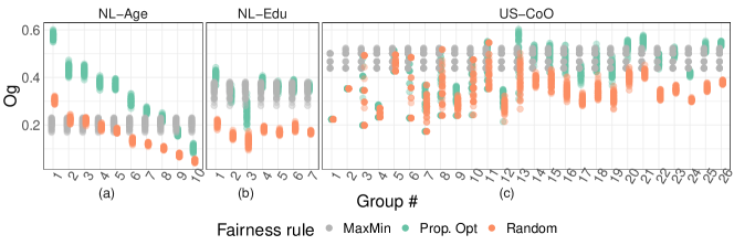
Figure 2: Minimum requirements for each group and scenario over bootstrapped arrival sequences.

6.2 Group fairness limitations of status quo approaches

We now discuss the group fairness of two algorithms that closely mimic status quo procedures: Rand and BP. Rand assigns each case randomly to a location with available capacity; this closely resembles status quo operations in the absence of optimization. BP (see Section 3) is similar to deployed algorithms (see [BP22, AGP⁺21]) and closely approximates the employment-maximizing (without fairness constraints) hindsight-optimal assignment, referred to as $\mathrm{OPT}$. Although we discuss results in this section with respect to BP, similar insights arise for $\mathrm{OPT}$ (see Appendix A.3).

To measure group fairness, for a group $g$ and a sample path $\boldsymbol{\omega}$, we define the fairness ratio as

$$\textsc{FR}_{g}(\boldsymbol{\omega})\triangleq\frac{\alpha_{g}(\boldsymbol{\omega})}{O_{g,\mathcal{F}}(\boldsymbol{\omega})}.$$

This is related to, but not the same as, ex-post $g-$regret, and allows for a more interpretable comparison across contexts. A fairness ratio of 0.5 means that a group’s average employment score is half of its minimum requirement prescribed by $\mathcal{F}$, and a fairness ratio greater than one implies that employment levels are higher than the requirement. To aggregate across groups, we define the minimum fairness ratio $\textsc{FR}(\boldsymbol{\omega})\triangleq\min_{g}\textsc{FR}_{g}(\boldsymbol{\omega})$ and its sample average $\textsc{FR}=\frac{1}{50}\sum_{n=1}^{50}\textsc{FR}(\boldsymbol{\omega}_{n})$.

We first examine the performance of Rand under our three fairness rules (see top of Figure 3). Recall that, for case $t$, their minimum requirement under the Random fairness rule is equivalent to their expected outcome under Rand. Rand, however, must choose a single location for each case. Thus, the fairness ratios are generally centered around one, but $\textsc{FR}_{g}(\boldsymbol{\omega})$ for a single sample path can be large, especially for the small groups in the US-CoO scenario. Results follow similar patterns under the Proportionally Optimized fairness rule but are more unfair. This arises because the minimum requirement obtained under the Proportionally Optimized fairness rule is larger than that obtained under the Random fairness rule (see Figure 2), especially for large groups.

We then consider the MaxMin fairness rule (see again top of Figure 2). In the NL-Age scenario, Rand is usually fair for groups 1-3, but not for 4-10 ($\textsc{FR}_{g}(\boldsymbol{\omega})$ of up to 0.8). The observation that fairness decreases with age is again a consequence of the higher overall employment rates among younger populations. To build intuition, consider a stylized example where younger groups are highly employable at any location, but older groups have only one location with high employment scores. In order to achieve their MaxMin requirement, a disproportionate number (relative to group size) of older cases would need to be assigned to that location. Since, under Rand, their expected allotment in each location is exactly proportional to their size, they do not meet their minimum requirement. In the NL-Edu and US-CoO scenarios, results under the MaxMin fairness rule reflect those obtained under proportionally optimized fairness.

Finally, we discuss the fairness ratio of BP (bottom of Figure 3). For most groups (with the exception of certain small groups in the US-CoO scenario) BP is fair under the Random fairness rule. However, BP may be unfair for certain groups under both the MaxMin and Proportionally Optimized fairness rules. The fairness ratio is particularly low under MaxMin fairness for groups 9 and 10 in the NL-Age scenario, group 3 in the NL-Edu scenario, and various groups in the US-CoO scenario. Therefore, although BP appears to be fairer than Rand for most groups, BP can be unfair, sometimes extremely so, for some groups.

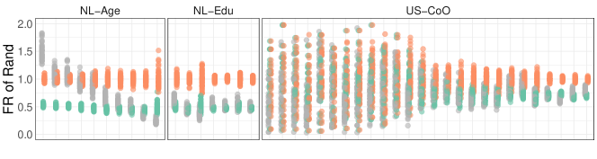
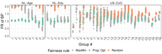
Figure 3: $\textsc{FR}_{g}(\boldsymbol{\omega})$ of Rand and BP with respect to the three fairness rules in each scenario.

6.3 Group and global objectives of our algorithms

We now compare the fairness ratio and total employment score achieved by our algorithms (ABP and CBP) with the above status-quo approaches (Rand and BP) and the optimal offline benchmarks, $\text{OFFLINE}_{\mathcal{F}}$ and $\mathrm{OPT}$. We note that the latter rely on knowledge of the sample path $\boldsymbol{\omega}$ and thus are not implementable in practice but are useful as upper bounds for the total employment with and without fairness constraints, respectively.

Group fairness. Our analysis finds that each of our benchmarks exhibits a FR less than 0.5 in multiple instances (see Figure 4). In comparison, ABP and/or CBP improve upon FR in all instances, often dramatically, with the exception of the NL-Edu scenario under the Proportionally Optimized fairness rule. In this instance, OPT already has very large FR and therefore BP, ABP, and CBP perform similarly, and are all less fair than OPT due to the efficiency loss from making decisions online. Focusing on the scenarios from the Netherlands (which have only large groups, see Table 1), ABP has a minimum FR of 91%; in the US-CoO scenario that does contain small groups, CBP has a minimum FR of 92%. More generally, in line with our expectations from Theorems 2 and 4, ABP and CBP perform similarly well on FR when all groups are large, and it is only in the US-CoO scenario that CBP does significantly better.

The existence of small groups in the US-CoO scenario warrants a more detailed investigation of each algorithm’s FR. Focusing on small (less than 10 arrivals) and large groups (more than 100), we find that CBP dramatically reduces the proportion of sample paths with $\textsc{FR}_{g}(\boldsymbol{\omega})<1$ for small groups. Among large groups, CBP results in a larger proportion of sample paths with $\textsc{FR}_{g}(\boldsymbol{\omega})<1$ than ABP, though the magnitude is small in these cases (see Table 3 in Appendix A.4 for more details). This demonstrates a trade-off: ABP guarantees group-fairness for large groups, whereas CBP introduces inefficiencies to help all groups meet their minimum requirement.

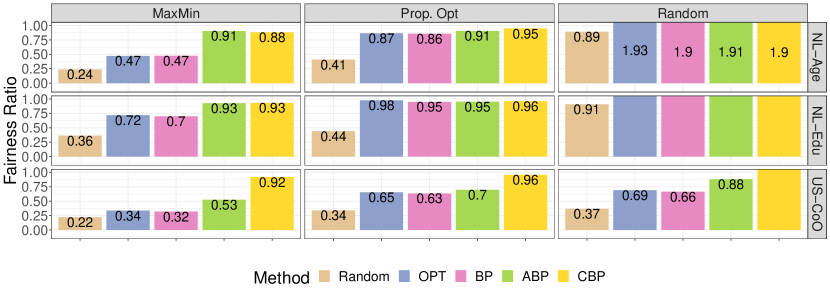
Figure 4: Average fairness ratio under the three fairness rules for each scenario, aggregated across 50 bootstrapped sample paths. We note that, unlike ABP and CBP, the Random, OPT, and BP algorithms are independent of the chosen fairness rule.

Global objective. The last goal of our data-driven exploration is to compare the global objective of the approaches and benchmarks (see Table 2). By comparing $\text{OFFLINE}_{\mathcal{F}}$ to OPT we can characterize the loss in total employment necessary to accommodate group fairness. With just one exception, $\text{OFFLINE}_{\mathcal{F}}$ always obtains at least 99% of $\mathrm{OPT}$, showing that group fairness may come at a low cost. In some cases, this occurs because the minimum requirements are met “for free”, i.e., the fairness constraints are naturally fulfilled when maximizing total employment (see Figure 4). A second and more nuanced reason relates to patterns in the employment score vectors. When these are highly correlated, yet slightly offset, swapping the assignment of two cases in different groups may yield small changes in total employment but large changes in average group employment.

All of the online methods (BP, ABP, and CBP) average at least 95% of the total employment level under OPT. The ordering between these three is unsurprising since BP optimizes solely for total employment while ABP and CBP introduce inefficiencies with the goal of increasing degrees of fairness. However, ABP loses no more than 2% efficiency compared to BP, and CBP loses no more than 1% efficiency compared to ABP. In the NL-Edu scenario under the Proportionally Optimized fairness rule, where OPT results in high FR, ABP and CBP not only result in the same FR as BP (discussed above), but also produce the same total employment (Table 2). Therefore, as desired, when fairness is not a concern our algorithms revert back to maximizing total employment. In other scenarios, these small losses in efficiency should be considered alongside the improvement in fairness that they achieve. Indeed, for US-CoO under the Random fairness rule, CBP and ABP are as efficient as BP while significantly improving fairness ratios.

	NL-Age				NL-Edu				US-CoO
Rule:	MaxMin	PrOpt	Random		MaxMin	PrOpt	Random		MaxMin	PrOpt	Random
Rand	0.46	0.46	0.46		0.46	0.46	0.46		0.67	0.67	0.67
CBP	0.95	0.97	0.98		0.97	0.97	0.98		0.97	0.98	0.99
ABP	0.96	0.98	0.98		0.98	0.98	0.98		0.98	0.99	0.99
BP	0.98	0.98	0.98		0.98	0.98	0.98		0.99	0.99	0.99
OFFLINEF	0.97	1.00	1.00		0.99	1.00	1.00		0.99	1.00	1.00

Table 2: Average ratio of total employment achieved under each algorithm compared to OPT.

6.4 Practical Implications

Our work aims to contribute to the algorithmic toolbox of GeoMatch, a decision support tool developed by the Immigration Policy Lab (IPL) at Stanford University. GeoMatch builds on methods first proposed in [BFH⁺18]. Currently deployed or in development in multiple countries, the GeoMatch tool is tailored to each country context and provides location recommendations to human case workers who make the final geographic placement decision. In what follows we discuss the practical requirements that guided the development of our approach.

Partner organizations would interact with the algorithms proposed in the paper in two ways: 1) the partner provides the definition for the groups and the fairness rule and 2) case workers at the partner organization receive location recommendations. Thus, both interactions should be relatively simple and explainable. The methods in this paper do not change interaction (2) relative to the status quo (although we note that the explanation for the recommendations may need to be slightly modified for these algorithms compared to the currently deployed algorithm of [BP22]; however, the main complexity in explaining recommendations stems from the core idea of opportunity costs in online resource allocation more generally. The added complexity of ABP and BP is thus marginal within the space of online algorithms). We have made interaction (1) as straightforward as possible by introducing a simple framework for fairness rules, and algorithms that can be adapted to a large set of fairness rules.

7 Conclusions

In this paper, we introduced the first formal approach to incorporating group fairness into the dynamic refugee assignment problem. Our approach explicitly addresses the practical needs of refugee resettlement stakeholders by offering flexibility to policy makers when specifying the notions of group fairness desiderata they wish to attain. Moreover, we developed new assignment algorithms that are guaranteed to achieve strong global and group-level performance guarantees for any feasible definition of group fairness chosen by the policy maker. Finally, through extensive numerical experiments on multiple real-world data, we showed that our online algorithms can achieve desired group-level fairness outcomes with very small changes in global performance.

Both our theoretical and empirical results demonstrate the performance of our two proposed algorithms, ABP and CBP. While BP achieves a higher overall average employment rate than our proposed methods, this results in unfair outcomes for certain groups under various fairness rules. In some settings, BP gets “lucky” and achieves group fairness, for example when the minimum requirements are quite loose as in the NL-Edu scenario under the Random fairness rule. ABP improves upon BP in terms of fairness, working well when all groups are relatively large and obtaining an overall average employment score within 2% of BP on real-world data. CBP sacrifices some efficiency ($\sim 1\%$) relative to ABP in order to achieve fairer outcomes for all groups regardless of size. Therefore, it is a natural choice in settings with small groups.

Our work opens up a number of promising directions for future research:

• In this paper, we make the assumption that each individual belongs in a unique group; this makes sense when the group definition is based on a single attribute (country of origin, age, educational level, gender) and is important for our algorithms to know how to assign reserves. That said, in practice, refugees and asylum seekers have multiple attributes and their profile is defined as an intersection of the respective subgroups. Designing algorithms that account for such intersectional groups is a fundamental direction for future work.

• In this paper, we assume that a case consists of a single individual and our results can easily extend to the case where cases have multiple individuals who all belong to the same group. That said, many families consist of members of different gender, educational level, age, etc. Since families must be assigned to the same location, our methods do not readily apply to settings with within-case group-heterogeneity and this is an important extension.

• Although our framework is flexible enough to incorporate various fairness rules, these rules need to be defined as a minimum requirement on the average performance on the group. This precludes fairness rules that aim to optimize, say, for the performance achieved by the $10$th-percentile of the group, which may be a meaningful statistic as it disallows a few good outcomes to outweigh the experience of the majority of the group members. Providing results that account for more general fairness rules can thus be a useful direction for future work.

Finally, we hope that future work may extend our algorithmic techniques for achieving group fairness that is specified by an ex-post minimum requirement (Section 2.2) to various other public policy settings in which individuals must be assigned dynamically (e.g., in health care and housing). More broadly, this work is a concrete example of how AI can be used to achieve complex and socially beneficial policy goals—an area with significant opportunity for future research.

Appendix A Supplementary material for numerical results (Section 6)

A.1 Estimation

The outcomes, $w_{tj}$ for case $t$ at location $j$, are estimated according to the methodology proposed in [BFH⁺18]. Thus, we refer the reader to [BFH⁺18] for more details, but highlight the key information in what follows.

First, separate machine learning (ML) models are trained for each location $j$ using historical administrative data for refugees that were previously assigned to location $j$. The covariates used in the ML models consist of individual-level features such as country of origin, age, language skills, education, family size, sex, etc. When a new case $t$ arrives, the predicted outcome vector $(w_{t1},...,w_{tM})$ is generated by first applying each of the $M$ machine learning models to every individual within case $t$. Then, the individual-level predictions are aggregated to a case-level prediction for every location by applying a particular mapping. For example, $w_{tj}$ may be the average predicted outcome among all individuals in case $t$. Alternatively, when the outcomes are binary (such as whether an individual has found employment), $w_{tj}$ could be the probability of at least one individual in case $t$ achieving a positive outcome. This paper uses the latter mapping.

In what follows, we provide structural properties of the estimates $w_{tj}$ in both the US and Netherlands contexts, as these properties can help provide context for the numerical results shown in Section 6.

For the US data, for fixed $t$, the average span—i.e., the difference between the maximum and minimum values—of $w_{tj}$ is 0.67 with standard deviation 0.12, and for fixed $j$ the average span of $w_{tj}$ is 0.56 with standard deviation 0.2. The span of average probability of employment across locations is 0.6. For the NL data, for fixed $t$, the average span of $w_{tj}$ is 0.43 with standard deviation 0.22, and for fixed $j$ the average span of $w_{tj}$ is 0.72 with standard deviation 0.18. Across locations, the span of the average probability of employment is 0.3.

There is also correlation between the predicted outcomes for cases within the same group. This is because all of the group definitions in the paper (country of original, age, and education) are covariates used to in the ML models. For the US data (where groups are defined by country of origin), the average correlation within a group is 0.82, compared to the average correlation across the entire dataset of 0.76. For the NL data with groups defined by age, the average correlation within a group is 0.52 (with standard deviation .03 across groups) compared to 0.46 overall. When groups are defined by education, the average correlation within groups is 0.51 with standard deviation 0.04 across groups.

A.2 Algorithmic set-up

We now describe the details of the implementations of all online methods—BP, ABP, and CBP— used in Section 6.

ABP and CBP.

As described in Section 3, the parameters $\boldsymbol{\lambda}^{*}$ and $\boldsymbol{\mu}^{*}$ used in ABP and CBP (Algorithms 1 and 2) are found by solving $\min_{\boldsymbol{\lambda}>0,\boldsymbol{\mu}>0}\mathbb{E}\left[L(\boldsymbol{\mu},\boldsymbol{\lambda})\right]$ where

$$L(\boldsymbol{\mu},\boldsymbol{\lambda}) =\sum_{t=1}^{T}\max_{j\in\mathcal{M}}((1+\lambda_{g(t)})w_{t,j}-\mu_{j})+\sum_{j\in\mathcal{M}}\mu_{j}s_{j}-\sum_{g\in\mathcal{G}}\lambda_{g}O_{g}N(g,T).$$

Let the superscript $k$ index a sample path of arrivals. The minimization problem is approximated by solving the following sample-average approximation across $K$ sample paths:

$$\min_{\boldsymbol{\lambda}>0,\boldsymbol{\mu}>0} \sum_{k=1}^{K}\left(\sum_{t=1}^{T}z^{k}_{t}+\sum_{j\in\mathcal{M}}\mu_{j}s_{j}-\sum_{g\in\mathcal{G}}\lambda_{g}O^{k}_{g}N^{k}(g,T)\right)$$ (1)

s.t. $$z^{k}_{t}\geq((1+\lambda_{g^{k}(t)})w^{k}_{t,j}-\mu_{j})\;\forall j\in\mathcal{M},\;t\in\{1,...,T\}$$

where $O^{k}_{g}$ and $N^{k}(g,T)$ can be pre-computed offline for each sample path of arrivals and then treated as constants in Problem 1. Using the auxiliary variables $z_{t}^{k}$, Problem 1 is a linear program and thus computationally tractable.

After calculating $\boldsymbol{\lambda}^{*}$ and $\boldsymbol{\mu}^{*}$, Algorithm 1 can be implemented as described in Section 3. For Algorithm 2, we similarly compute $\boldsymbol{\lambda}^{*}$ and $\boldsymbol{\mu}^{*}$ and set $\mathrm{Cap}(\beta)=\infty$ and $\mathrm{Res}(\beta)=1$. Therefore, each group can use an unlimited amount of reserved capacity in theory, however each location only has one reserved unit of capacity.

For Algorithm 2, the value of $\Psi(g,t,\beta)$ is set in the following data-driven way: First, we find a confidence interval $[l_{g},u_{g}]$ for the number of remaining arrivals of each group $g$; this uses the fact that the number of remaining arrivals of each group $g$ follows a Binomial distribution with mean $(T-t)\bar{p}_{g}$. Specifically, we set $l_{g}=(T-t)\bar{p}_{g}-Z_{g}(0.9)$ and $u_{g}=(T-t)\bar{p}_{g}+Z_{g}(0.9)$ where $Z_{g}(x)$ denotes the inverse CDF of the group-specific Binomial distribution. Intuitively, for each $n\in[l_{g},u_{g}]$, we want to know: If there are $n$ remaining arrivals in group $g$ and they are all assigned to their highest-score (greedy) location, what is the chance this group will not meet its minimum requirement? For each $n\in[l_{g},u_{g}]$, we independently sample $n$ group $g$ arrivals $K$ times. For each of the $K$ length-$n$ vectors, $\{\mathbf{w}_{\tau}^{k(g)}\}_{\tau=1,...,n}$, we calculate $s_{g}^{k}:=\sum_{\tau=1}^{n}(\max_{j}w^{k(g)}_{\tau j}-\mathbb{E}[O_{g}])$ for $k=1,...,K$. Finally, we calculate the 10% quantile of $[s_{g}^{1},...,s_{g}^{K}]$ and use this value, $q(n,g)$, to set $\Psi(g,t,\beta)=\min_{n\in[l_{g},u_{g}]}q(n,g)$. This effectively lower bounds $\sum_{\tau\in\mathcal{A}(g,T)\setminus\mathcal{A}(g,t)}(\max_{j}w_{\tau j}-\mathbb{E}[O_{g}])$ as desired.

BP.

To determine the parameters $\boldsymbol{\mu}^{*}$ used in BP, we compute a sample average of the optimal dual values of the continuous relaxation of OPT. This is also equivalent to the approach described above for ABP without a fairness constraint (e.g. achieved by setting $O_{g}=0$ for all groups $g$).

A.3 Additional figures for Section 6.2

Figure 5 shows $\textsc{FR}_{g}(\boldsymbol{\omega})$ for each group under OPT using our three fairness rules. This can be compared to Figure 3 which shows $\textsc{FR}_{g}(\boldsymbol{\omega})$ for Rand and BP.

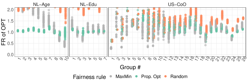
Figure 5: $\textsc{FR}_{g}(\boldsymbol{\omega})$ achieved by OPT with respect to the three fairness targets for each scenario.

A.4 Additional figures and tables for Section 6.3

Figure 6 shows group-level results for the ABP and CBP algorithms, analogous to Figure 3 that was shown for Rand and BP.

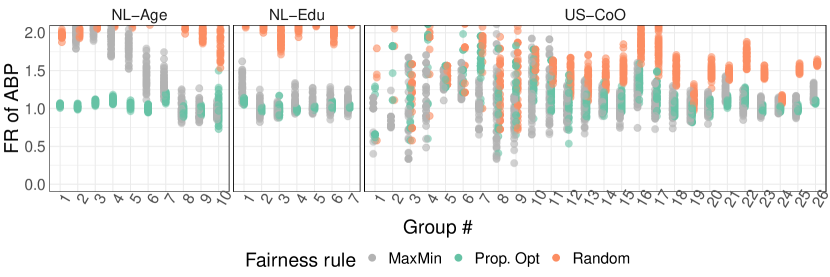
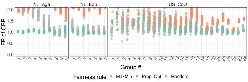
Figure 6: $\textsc{FR}_{g}(\boldsymbol{\omega})$ achieved by ABP and CBP with under our three fairness rules.

		% positive regret			Avg fairness ratio
Group	Size	BP	ABP	CBP	BP	ABP	CBP
1	small	1.00	0.91	0.00	0.59	0.65	0.00
2	small	0.00	0.00	0.00	0.00	0.00	0.00
3	small	0.41	0.39	0.02	0.76	0.76	0.99
4	small	0.02	0.02	0.02	0.90	0.60	0.91
5	small	0.00	0.00	0.00	0.00	0.00	0.00
6	small	0.00	0.00	0.00	0.00	0.00	0.00
7	small	0.00	0.00	0.00	0.00	0.00	0.00
8	small	0.41	0.43	0.00	0.82	0.80	0.00
9	small	0.54	0.35	0.06	0.82	0.85	0.98
10	small	0.00	0.02	0.02	0.00	0.87	0.93
11	small	0.00	0.15	0.04	0.00	0.98	0.93
12	small	0.00	0.28	0.02	0.00	0.88	1.00
13	small	0.26	0.28	0.10	0.94	0.94	0.97
14	medium	0.14	0.12	0.18	0.98	0.96	0.97
15	medium	0.00	0.14	0.02	0.00	0.97	0.98
16	medium	0.00	0.00	0.00	0.00	0.00	0.00
17	medium	0.00	0.10	0.04	0.00	0.95	0.96
18	medium	0.04	0.48	0.16	0.97	0.94	0.96
19	medium	1.00	0.54	0.34	0.83	0.93	0.97
20	medium	0.02	0.36	0.18	0.98	0.96	0.98
21	medium	0.00	0.00	0.00	0.00	0.00	0.00
22	medium	0.00	0.00	0.06	0.00	0.00	0.99
23	large	0.34	0.66	0.74	0.98	0.98	0.98
24	large	1.00	0.56	0.82	0.82	0.98	0.98
25	large	0.06	0.74	0.78	0.99	0.98	0.98
26	large	0.00	0.00	0.00	0.00	0.00	0.00

Table 3: Percentage of instances (out of 50) with positive regret, and average fairness ratio conditional on having positive regret. “Small” groups are those with fewer than 10 arrivals. “Medium” groups are those with between 10-100 arrivals, and “large” groups have over 100 arrivals. Note: This table is based on US data using the Proportional Optimized fairness rule.

A.5 Evaluation beyond i.i.d. based on a single historical trace (Section 6.3)

In this section we demonstrate the performance of our algorithms in a setting that most closely resembles the real world. In reality, non-stationarities arise due to changing arrival patterns of refugees with certain characteristics (e.g., one country of origin might have a spike of arrivals in a given month), and due to changing economic conditions in the host country. To get a sense for the level of non-stationarity, we estimated $U$ for each scenario by splitting 2015 and 2016 into quarters and empirically estimating the value of $U$. In the Netherlands, we found that $U\leq 1.7$ in both years with one exception: with groups defined by Education, there is one group in one quarter of 2016 that causes $U$ to be equal to $7.5$. For the US, there are many small groups that may have no arrivals in a given quarter and thus $U$ cannot not be estimated. Among the groups where it could be estimated, we find that $U\leq 4.5$ both years.

We treat the 2016 arrivals—in the order that they actually arrived—as the test cohort. Therefore, the arrival sequence no longer satisfies an i.i.d. assumption. All parameters used in the algorithms (e.g., $\boldsymbol{\lambda}^{*}$, $\boldsymbol{\mu}^{*}$, and $\mathbb{E}[O_{g}]$) are determined using the 2015 cohort of arrivals. When running the algorithms, the only knowledge that the algorithm has about the 2016 arrivals is the total number of 2016 arrivals and the capacity vector for 2016. These assumptions reflect the information known in reality.

There is one subtle complexity. Suppose there are certain groups which are present in the 2016 arrival cohort that were not present in the 2015 arrival cohort. This means that we cannot estimate $\lambda_{g}^{*}$ for a group $g$ in this situation. This is not an issue in the NL-Edu or NL-Age scenarios, but is an issue in the US-CoO scenario. We propose handling the issue in the following way. If there is a large group $g$ that arrives in 2016 and not in 2015, it is likely that the policymaker will have prior knowledge about this group. For example, there may have been a policy that prohibited this group from arriving in 2015, but policy changes allow for their arrival in 2016. With this prior knowledge, we could use data-driven approaches to estimate $\lambda_{g}^{*}$ for this group. For example, we could generate employment probability predictions for simulated arrivals from this group and add them to the 2015 arrival cohort before computing the parameters of the algorithms.

Now consider a second situation in which refugees from a group $g$ arrive in 2016, but had no arrivals in 2015, and the policymakers did not have prior knowledge about this change. In this case, it is likely that the group is quite small. For example, if a particular group has, on average, only a handful of arrivals, it is likely there are certain years where the group will have zero arrivals, and policymakers might not pay special attention to this. In this situation, we propose either a) using older data that includes arrivals from this group when determining the parameters of the algorithm or b) assigning arrivals to this group to their greedy locations. Because these groups are likely to be quite small, this will not greatly impact the performance of the algorithm. For the numerical results of this section, we take this approach, and assign any arrivals from a group that did not appear in 2015 to their greedy location (among those with remaining capacity).

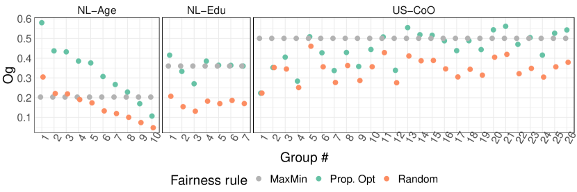
Figure 7: Minimum requirements for the 2016 arrival cohort.

	NL-Edu				NL-Age				US-CoO
Rule:	MaxMin	PrOpt	Random		MaxMin	PrOpt	Random		MaxMin	PrOpt	Random
Rand	0.46	0.46	0.46		0.46	0.46	0.46		0.67	0.67	0.67
CBP	0.94	0.95	0.96		0.93	0.94	0.96		0.89	0.91	0.92
ABP	0.94	0.96	0.96		0.96	0.96	0.96		0.91	0.92	0.92
BP	0.96	0.96	0.96		0.96	0.96	0.96		0.92	0.92	0.92
OfflineF	0.98	1.00	1.00		0.99	1.00	1.00		0.98	1.00	1.00

Table 4: Efficiency of methods in the “real-world” scenario.

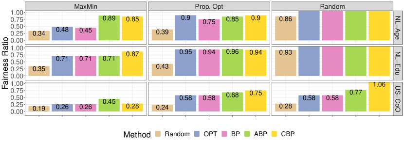
Figure 8: Fairness ratio (aggregated by min) obtained in the “real-world” scenario. Note: Unlike ABP and CBP, the Random, OPT, and BP algorithms are independent of the chosen fairness rule.

Appendix B Infeasibility of Resolving Methods (Section 1.2)

It is natural to wonder whether resolving techniques from the literature on online resource allocation are immediately applicable to our setting with group fairness constraints. In this appendix, we demonstrate through an example that vanilla applications of these techniques may fail if they require solving infeasible optimization problems. We consider the Bayes Selector algorithm [VB21, algorithm 1]. The MinDiscord algorithm of [BP22], which was developed in the context of refugee assignment, follows a similar idea to assign refugees but without group fairness constraints.

Upon the arrival of case $t$, the DM observes the first $t$ arrivals $\hat{\boldsymbol{\theta}}_{1},\ldots,\hat{\boldsymbol{\theta}}_{t}$ and has assigned the initial $t-1$ arrivals whose assignment vectors are given by $\hat{\boldsymbol{z}}_{1},\ldots,\hat{\boldsymbol{z}}_{t-1}$. Then the DM samples a list of $K$ future sample paths $\{\boldsymbol{\omega}^{k}_{t}=(\boldsymbol{\theta}^{k}_{t+1},\ldots,\boldsymbol{\theta}^{k}_{T})\}_{k\in[K]}$ with $K$ being a hyper-parameter. The sampling is independent across paths and each feature vector $\boldsymbol{\theta}^{k}_{\tau}$ is sampled from the known probability distribution $\mathcal{P}_{\tau}$ for $\tau>t$. For each concatenated sample path $\hat{\boldsymbol{\omega}}^{k}_{t}=(\hat{\boldsymbol{\theta}}_{1},\ldots,\hat{\boldsymbol{\theta}}_{t},\boldsymbol{\theta}^{k}_{t+1},\ldots,\boldsymbol{\theta}^{k}_{T})$, the DM computes the optimal fractional assignment $\boldsymbol{\tilde{z}}^{k}$ to the offline problem $O^{\star}_{\mathcal{F}}(\hat{\boldsymbol{\omega}}^{k}_{t})$ in ($\text{OFFLINE}_{\mathcal{F}}$), with an additional constraint that assignments of the first $t-1$ cases are consistent, i.e., $\boldsymbol{\tilde{z}}^{k}_{\tau}=\hat{\boldsymbol{z}}_{\tau}$ for $\tau<t$. Case $t$ is assigned to the location with the highest probability among these optimal assignments, that is, location $J(t)\in\arg\max_{j\in\mathcal{M}}\sum_{k\in[K]}\tilde{z}^{k}_{t,j}$.

Since the group fairness constraints depend on sample paths, the offline problem $O^{\star}_{\mathcal{F}}(\hat{\boldsymbol{\omega}}_{t}^{k})$ may be infeasible because conducted assignment decisions are induced by other sample paths and no future assignment decisions can satisfy the group fairness constraints for this sample path. This is not an issue when there are only capacity constraints as these constraints do not vary across sample paths. The following proposition formalizes this intuition.

Proposition 4.

For any even $T\geq 1000$, there exists a setting such that with probability at least $0.0261$, for the second arrival, Bayes Selector with any hyper-parameter $K\geq 1$ must solve an infeasible offline problem during its run-time.

Proof.

Suppose $T$ is an even number at least $1000$. Consider the following setting with $2$ locations $\{1,2\}$, and three groups $\{A,B,C\}$. Locations have capacity $s_{1}=T/2,s_{2}=T/2$. Group arrival probabilities are $p_{A}=0.4,p_{B}=0.6-1/T,p_{C}=1/T$. Scores of arrivals to locations are determined by their groups such that $w_{t,1}=1,w_{t,2}=0.5$ if $t$ is in group $A$; $w_{t,1}=0.5,w_{t,2}=0$ if $t$ is in group $B$; and $w_{t,1}=w_{t,2}=0$ if $t$ is in group $C$. The fairness rule is MaxMin (Example 3).

Fix the hyper-parameter $K\geq 1$. Let us simulate the algorithm from case $1$. With probability $p_{A}\geq 0.4$, the first case is from group $A$; denote its feature by $\hat{\boldsymbol{\theta}}_{1}$. Consider the algorithm for case $1$. Denote the set of paths sampled by the DM by $\Omega_{1}=\{\boldsymbol{\omega}_{1}^{k}=(\boldsymbol{\theta}^{k}_{2},\ldots,\boldsymbol{\theta}^{k}_{T})\}_{k\in[K]}$. Define $\mathcal{S}_{1}$ as a set of sample paths from case $2$ to case $T$ such that there is a group $C$ arrival and the number of group $A$ arrivals is at most $0.5T-1$, that is, $\mathcal{S}_{1}=\{(\boldsymbol{\theta}_{2},\ldots,\boldsymbol{\theta}_{T})\colon\sum_{t=2}^{T}\mathbbm{1}\left(g(\boldsymbol{\theta}_{t})=C\right)\geq 1,\sum_{t=2}^{T}\mathbbm{1}\left(g(\boldsymbol{\theta}_{t})=A\right)\leq 0.5T-1\}$. For any $\boldsymbol{\omega}_{1}^{k}\in\mathcal{S}_{1}$, consider the concatenated sample path $\hat{\boldsymbol{\omega}}_{1}^{k}=(\hat{\boldsymbol{\theta}}_{1},\boldsymbol{\omega}_{2}^{k})$. We know there is a group $C$ arrival and the number of group $A$ arrivals is at most $T/2$. Since the fairness rule is MaxMin, having a group $C$ arrival removes fairness constraints for all groups as cases from group $C$ always have score zero. The optimal fractional assignment $\tilde{\boldsymbol{z}}^{k}$ of $O^{\star}_{\mathrm{maxmin}}(\hat{\boldsymbol{\omega}}_{1}^{k})$ then assigns all group $A$ arrivals to location $1$ to maximize the total score. Therefore, if $\boldsymbol{\omega}_{1}^{k}\in\mathcal{S}_{1}$, we must have $\tilde{z}^{k}_{1,1}=1$ since the first case is of group $A$.

Let $\mathcal{E}_{1}$ be the event that more than half of the sample paths in $\Omega_{1}$ are in $\mathcal{S}_{1}$. If $\mathcal{E}_{1}$ holds, we have $\sum_{k=1}^{K}\tilde{z}_{1,1}^{k}>0.5>\sum_{k=1}^{K}\tilde{z}_{1,j}^{k}$ for $j=2,3$ and thus the algorithm will assign the first case to location $1$. To lower bound the probability of $\mathcal{E}_{1}$, we first upper bound the probability that $\boldsymbol{\omega}_{1}^{k}\not\in\mathcal{E}_{1}$ for any $k$ by

$$\mathbb{P}\{\boldsymbol{\omega}_{1}^{k}\not\in\mathcal{E}_{1}\} \leq\mathbb{P}\left\{g(\boldsymbol{\theta}_{t}^{k})\neq C,\forall t\geq 2\right\}+\mathbb{P}\left\{\sum_{t=2}^{T}\mathbbm{1}\left(g(\boldsymbol{\theta}_{t}^{k})=A\right)\geq 0.5T\right\}$$

$$\leq(1-p_{C})^{T-1}+\exp\left(\frac{-2(0.1T)^{2}}{T}\right)\leq 0.4+\exp(-20)\leq 0.41$$

which uses Hoeffding Inequality (Fact 3) and the fact that $p_{C}=1/T$ and $T\geq 1000$. As a result, $\mathbb{P}\{\boldsymbol{\omega}_{2}^{k}\in\mathcal{S}_{1}\}\geq 0.59$. Since sample paths are generated independently and any one sample path is more likely than not in $\mathcal{S}_{1}$, we can lower bound the probability that more than half of sample paths of $\Omega_{1}$ are in $\mathcal{S}_{1}$ by at least $0.25$ (the worst case is $K=2$).

Consider the second arrival, i.e., one with feature $\hat{\boldsymbol{\theta}}_{2}$. Condition on $\mathcal{E}_{1}$ and the event that the second arrival is not from group $C$. We know $\mathbb{P}\{g(\hat{\boldsymbol{\theta}}_{1})=A,\mathcal{E}_{1},g(\hat{\boldsymbol{\theta}}_{2})\neq C\}=p_{A}(1-p_{C})\mathbb{P}\{\Omega_{1}\}\geq 0.09$ since they are independent. Let $\Omega_{2}=\{\boldsymbol{\omega}_{2}^{k}\}_{k\in[K]}$ be the paths sampled by the algorithm. Define $\mathcal{S}_{2}$ to be the set of sample paths from case $3$ to case $T$ such that there is no group $C$ arrival and the number of group $B$ arrivals is at least $T/2$, i.e., $\mathcal{S}_{2}=\{(\boldsymbol{\theta}_{3},\ldots,\boldsymbol{\theta}_{T})\colon\sum_{t=3}^{T}\mathbbm{1}\left(g(\boldsymbol{\theta}_{t})=C\right)=0,\sum_{t=3}^{T}\mathbbm{1}\left(g(\boldsymbol{\theta}_{t})=B\right)\geq 0.5T\}$. Suppose that for some $k$, $\boldsymbol{\omega}_{2}^{k}\in\mathcal{S}_{2}$. Since there is no group $C$ arrival, the MaxMin fairness rule requires assigning as many group-$B$ arrivals as possible to location $1$ to increase the average score of group $B$, which is always no greater than that of group $A$. As a result, since the number of group $B$ arrivals is at least $T/2$ for sample paths in $\mathcal{S}_{2}$, any feasible assignment to the offline problem $O_{\mathrm{maxmin}}^{\star}(\hat{\boldsymbol{\omega}}_{2}^{k})$ must assign all location $1$ to group $B$ arrivals to satisfy its fairness constraint. However, as the first case of group $A$ is assigned to location $1$ and this decision is irrevocable, the offline problem $O_{\mathrm{maxmin}}^{\star}(\hat{\boldsymbol{\omega}}_{2}^{k})$ must be infeasible when $\boldsymbol{\omega}_{2}^{k}\in\mathcal{S}_{2}$.

We next lower bound the probability that $\boldsymbol{\omega}_{2}^{1}\in\mathcal{S}_{2}$ by

$$\mathbb{P}\{\boldsymbol{\omega}_{2}^{1}\in\mathcal{S}_{2}\} \geq\mathbb{P}\left\{g(\boldsymbol{\theta}_{t}^{1})\neq C,\forall t\geq 3\right\}-\mathbb{P}\left\{\sum_{t=3}^{T}\mathbbm{1}\left(g(\boldsymbol{\theta}_{t}^{k})=B\right)<0.5T\right\}$$

$$\geq(1-p_{C})^{T-1}-\exp\left(\frac{-2(0.08T)^{2}}{T}\right)\geq 0.3-\exp(-10)\geq 0.29.$$

As a result, condition on the event that $\{g(\hat{\boldsymbol{\theta}}_{1})=A\}\cap\mathcal{E}_{1}\cap\{g(\hat{\boldsymbol{\theta}}_{2})\neq C\}\cap\{\boldsymbol{\omega}_{2}^{1}\in\mathcal{S}_{2}\}$, which happens with probability at least $0.09*0.29=0.0261$ because of independence, Bayes Selector with any hyper-parameter $K\geq 1$ must solve an infeasible optimization problem. ∎

Appendix C Group Fairness Rules: Objectives and Assumptions (Section 2.3)

C.1 Impossibility of sample-path guarantees on ex-post $g$-regret

Let $\Phi(x)$ be the standard normal distribution. We need the following statement of Berry-Esseen Theorem adopted from Theorem 3.4.17 of [Dur19].

Fact 1.

Let $X_{1},X_{2},\ldots$ be i.i.d. with $\mathbb{E}\left[X_{i}\right]=0,\mathbb{E}\left[X_{i}^{2}\right]=\sigma^{2}$ and $\mathbb{E}\left[|X_{i}|^{3}\right]=\rho<\infty$. If $F_{n}(x)$ is the distribution of $(X_{1}+\cdots+X_{n})/\sigma\sqrt{n}$ then for every $x$, $|F_{n}(x)-\Phi(x)|\leq 3\rho/(\sigma^{3}\sqrt{n})$.

The following proposition shows that one cannot hope for vanishing ex-post $g$-regret (or competitive ratio) for arbitrary fairness rules. This motivates our weakening of the ex-post requirement.

Proposition 5.

There exists a constant $C>0$ such that, for any $T=100K$ with sufficiently large integer $K$, we can construct a problem setting and a fairness rule $\mathcal{F}$ with the property that for any non-anticipatory algorithm, with probability at least $C$, we must have

• high ex-post group regret: $\max_{g\in\mathcal{G}}\left(O_{g,\mathcal{F}}(\boldsymbol{\omega})-\alpha_{g}(\boldsymbol{\omega})\right)\geq 0.235$;

• low ex-post multiplicative approximation: $\min_{g\in\mathcal{G}}\frac{\alpha_{g}(\boldsymbol{\omega})}{O_{g,\mathcal{F}}(\boldsymbol{\omega})}\leq 0.53$.

Proof.

Fix $T=100K$ for $K\geq\frac{12}{\Phi(-25)^{2}}$ and let $C=\frac{(1-4e^{-4})\Phi(-25)}{2}>0$. Consider a setting with $M=2$ locations each with capacity $\frac{T}{2}$. There are two groups, each with equal arrival probabilities $p_{1}=p_{2}=0.5$. For every case $t$, the employment scores are given by $w_{t,1}=1,w_{t,2}=0$. The fairness rule $\mathcal{F}$ is defined as follows. For a sample path $\boldsymbol{\omega}$, the DM observes the number of arrivals of each group and assigns as many arrivals as possible of the larger group to the good location to set the required score. That is, if group $1$ has more or equal arrivals than group $2$, then $O_{1,\mathcal{F}}(\boldsymbol{\omega})=\frac{T}{2N(1,T)},O_{2,\mathcal{F}}(\boldsymbol{\omega})=0$; otherwise, $O_{1,\mathcal{F}}(\boldsymbol{\omega})=0,O_{2,\mathcal{F}}(\boldsymbol{\omega})=\frac{T}{2N(2,T)}$.

Fix a non-anticipatory algorithm. The algorithm could be randomized whose randomness is independent of the case arrival process. We assume the probability space is extended to include the randomness of the algorithm. Define $\tilde{R}(\boldsymbol{\omega})$ to be $\max\left(O_{1,\mathcal{F}}(\boldsymbol{\omega})-\alpha_{1}(\boldsymbol{\omega}),O_{2,\mathcal{F}}(\boldsymbol{\omega})-\alpha_{2}(\boldsymbol{\omega})\right)$ and let the multiplicative approximation (fairness ratio) be $\mathrm{FR}(\boldsymbol{\omega})=\max_{g\in\mathcal{G}}\frac{O_{g,\mathcal{F}}(\boldsymbol{\omega})-\alpha_{g}(\boldsymbol{\omega})}{O_{g,\mathcal{F}}(\boldsymbol{\omega})}.$ We next show that with probability at least $C$, we have $\tilde{R}(\boldsymbol{\omega})\geq 0.235$ and $\mathrm{FR}(\boldsymbol{\omega})\leq 0.53$.

Recall that $N(g,t)$ is the number of arrivals of group $g$ up to round $t$. Let $Q=0.97T=97K$. By Hoeffding’s Inequality (Fact 3), we have $\mathbb{P}\{|N(1,Q)-\frac{Q}{2}|>20\sqrt{K}\}\leq 2\exp\left(\frac{-400K}{97K}\right)\leq 2e^{-4}$. Similarly, we have $\mathbb{P}\{|N(2,Q)-\frac{Q}{2}|>20\sqrt{K}\}\leq 2e^{-4}$. Define

$$\mathcal{S}=\left\{|N(1,Q)-\frac{Q}{2}|\leq 20\sqrt{K}\right\}\cap\left\{|N(2,Q)-\frac{Q}{2}|\leq 20\sqrt{K}\right\}.$$ (2)

Then by union bound we have $\mathbb{P}\{\mathcal{S}\}\geq 1-4e^{-4}$. In addition, under $\mathcal{S}$ we have $|N(1,Q)-N(2,Q)|\leq 40\sqrt{K}$. Define $X$ by the difference between numbers of arrivals of the two groups in rounds $Q+1$ to $T$. That is, $X=N(1,T)-N(1,Q)-(N(2,T)-N(2,Q))$. We know $X$ is the sum of $T-Q=3K$ Rademacher random variables. Then by Berry-Esseen Theorem (Fact 1), we have $|\mathbb{P}\{\frac{X}{\sqrt{3K}}\leq a\}-\Phi(a)|\leq\sqrt{\frac{3}{K}}$ for any real value $a$. Taking $a=-25$ leads to $\mathbb{P}\{X\leq-41\sqrt{K}\}\geq\Phi(-25)-\sqrt{\frac{3}{K}}\geq\frac{1}{2}\Phi(-25)$ since $K\geq\frac{12}{\Phi(-25)^{2}}$. By the symmetry of $X$, we have $\mathbb{P}\{X\geq 41\sqrt{K}\}=\mathbb{P}\{X\leq-41\sqrt{K}\}\geq\frac{1}{2}\Phi(-25)$.

Now define $A_{1}$ by the number of cases in group $1$ that are assigned to location $1$ by round $Q$. Note that both $A_{1}$ and $\mathcal{S}$ are independent of $X$ since they are in the filtration of rounds up to $Q$ and are independent of arrivals in rounds $Q+1$ to $T$. Condition on $\mathcal{S}$ defined in (2). Consider two scenarios:

• $A_{1}\geq 0.235T,X\leq-41\sqrt{K}$. In this scenario, we know there are more arrivals of group $2$ since $N(2,T)-N(1,T)\geq 41\sqrt{K}-40\sqrt{K}>0$. By the definition of the fairness rule $\mathcal{F}$, we have $O_{2,\mathcal{F}}(\boldsymbol{\omega})N(2,T)=0.5T$. However, since $A_{1}\geq 0.235T$, at least $0.235T$ capacity from location $1$ are assigned to group $1$. We must have $\alpha_{2}(\boldsymbol{\omega})N(2,T)\leq\frac{T}{2}-0.235T=0.265T$, so $\tilde{R}(\boldsymbol{\omega})\geq\frac{1}{N(2,T)}\left(O_{2}(\boldsymbol{\omega})N(2,T)-\alpha_{2}(\boldsymbol{\omega})N(2,T)\right)\geq\frac{0.235T}{T}=0.235$. In addition,

  $$\mathrm{FR}(\omega)\leq\frac{\alpha_{2}(\boldsymbol{\omega})N(2,T)}{O_{2}(\boldsymbol{\omega})N(2,T)}\leq\frac{0.265T}{0.5T}=0.53.$$

• $A_{1}<0.235T,X\geq 41\sqrt{K}$. Similar to the above scenario, we have that $N(1,T)-N(2,T)>0$ and thus $O_{1,\mathcal{F}}(\boldsymbol{\omega})N(1,T)=0.5T$. But since only $A_{1}$ cases from group $1$ are assigned to location $1$ up to round $Q$ and there are at most $T-Q=3K$ cases after round $Q$, the total score of group $1$ is at most $0.235T+0.03T=0.265T$. Therefore, under this scenario, $\tilde{R}(\boldsymbol{\omega})\geq\frac{1}{N(1,T)}\left(O_{1,\mathcal{F}}(\boldsymbol{\omega})N(1,T)-\alpha_{1}(\boldsymbol{\omega})N(1,T)\right)\geq\frac{1}{T}\left(0.5T-0.265T\right)=0.235$. In addition,

  $$\mathrm{FR}(\omega)\leq\frac{\alpha_{1}(\boldsymbol{\omega})N(1,T)}{O_{1}(\boldsymbol{\omega})N(1,T)}\leq\frac{0.265T}{0.5T}=0.53.$$

Summarizing the above two scenarios, we obtain that

$$\mathbb{P} \left\{\tilde{\mathcal{R}}(\boldsymbol{\omega})\geq 0.235,\mathrm{FR}(\boldsymbol{\omega})\leq 0.53\right\}$$

$$\geq\mathbb{P}\{\mathcal{S}\}\mathbb{P}\left\{\tilde{\mathcal{R}}(\boldsymbol{\omega})\geq 0.235,\mathrm{FR}(\boldsymbol{\omega})\leq 0.53\,\middle|\,\mathcal{S}\right\}$$

$$\overset{(a)}{\geq}\mathbb{P}\{\mathcal{S}\}\left(\mathbb{P}\left\{A_{1}\geq 0.235T,X\leq-41\sqrt{K}\,\middle|\,\mathcal{S}\right\}+\mathbb{P}\left\{A_{1}<0.235T,X\geq 41\sqrt{K}\,\middle|\,\mathcal{S}\right\}\right)$$

$$\overset{(b)}{=}\mathbb{P}\{\mathcal{S}\}\left(\mathbb{P}\left\{A_{1}\geq 0.235T\,\middle|\,\mathcal{S}\right\}\mathbb{P}\left\{X\leq-41\sqrt{K}\right\}+\mathbb{P}\left\{A_{1}<0.235T\,\middle|\,\mathcal{S}\right\}\mathbb{P}\left\{X\geq 41\sqrt{K}\right\}\right)$$

$$\overset{(c)}{=}\mathbb{P}\{\mathcal{S}\}\frac{\Phi(-25)}{2}\left(\mathbb{P}\left\{A_{1}\geq 0.235T\,\middle|\,\mathcal{S}\right\}+\mathbb{P}\left\{A_{1}<0.235T\,\middle|\,\mathcal{S}\right\}\right)$$

$$\overset{(d)}{=}\mathbb{P}\{\mathcal{S}\}\frac{\Phi(-25)}{2}\geq\frac{(1-4e^{-4})\Phi(-25)}{2}$$

where (a) is by the law of total probability and the fact that the two events have no intersection; (b) is by the independence between $X$ and the filtration up to round $Q$; (c) is by the result we obtained before that $|X|\geq 41\sqrt{K}$ happens with probability at least $\frac{\Phi(-25)}{2}$; (d) is because the two events are complement. We thus finish the proof. ∎

C.2 Impossibility of sample-path approximation of $\mathbb{E}_{\boldsymbol{\omega}^{\prime}}\left[O_{g,\mathcal{F}}(\boldsymbol{\omega}^{\prime})\right]$

We next show that the above issue cannot be solved by reverting to the expected minimum requirement $\mathbb{E}_{\boldsymbol{\omega}^{\prime}}\left[O_{g,\mathcal{F}}(\boldsymbol{\omega}^{\prime})\right]$ as a benchmark. In particular, there is an instance where no algorithm can obtain a constant fraction of this benchmark with high probability due to the presence of a small group. This motivates our definition of $g$-regret.

Proposition 6.

For any $T\geq 1$, we can construct a problem setting and a fairness rule $\mathcal{F}$ with the property that for any algorithm and constant $c\in(0,1)$, with probability at least $\frac{c}{18}$, we must have $\alpha_{g}(\boldsymbol{\omega})<c\mathbb{E}_{\boldsymbol{\omega}^{\prime}}\left[O_{g,\mathcal{F}}(\boldsymbol{\omega}^{\prime})\right]$ for some group $g$.

Proof.

Fix $T\geq 1$ and the constant $c\in(0,1)$. Consider $T$ arrivals from two groups, group $1$ and $2$, with $p_{1}=1/T,p_{2}=1-1/T$. There is one location with capacity $T$. The score $w_{t}$ of an arrival to the location is uniformly at random in $[0,1]$. On the one hand, we have

$$\mathbb{E}\left[O_{1}\right]\geq\mathbb{E}\left[O_{1},N(1,T)=1\right]=\sum_{t=1}^{T}\mathbb{E}\left[w_{t},g(t)=1,N(1,T)=1\right]=\frac{Tp_{1}(1-p_{1})^{T-1}}{2}\geq\frac{1}{6}$$

where the last inequality is because $(1-1/x)^{x-1}$ is a decreasing function over $x\geq 1$ and $\lim_{x\to\infty}(1-1/x)^{x-1}=e^{-1}$. On the other hand, define $T$ events $\mathcal{E}_{1},\ldots,\mathcal{E}_{T}$ where under $\mathcal{E}_{t}$, we have $g(t)=1,N(g,T)=1,$ and $w_{t}<\frac{c}{6}$. Then $\mathbb{P}(\mathcal{E}_{t})\geq\frac{c}{6}p_{1}(1-p_{1})^{T-1}$. Let $\mathcal{E}=\cup_{t}\mathcal{E}_{t}$. Note that since $\mathcal{E}_{t}$’s have no intersection, we have $\mathbb{P}\{\mathcal{E}\}\geq\frac{c}{6}Tp_{1}(1-p_{1})^{T-1}\geq\frac{c}{18}$. However, conditioning on $\mathcal{E}$, we must have $\alpha_{1}<\frac{c}{6}=c\mathbb{E}\left[O_{1}\right]$, which completes the proof. ∎

C.3 Impossibility of joint sample-path optimality and low group regret

Moving to global regret, we now show that having an ex-post sample-path benchmark $O^{\star}_{\mathcal{F}}(\boldsymbol{\omega})$ is conflicting with group fairness. In particular, achieving the optimal score while maintaining low group regret is impossible.

Proposition 7.

There exists a constant $C>0$ such that, for any $T=100K$ with sufficiently large integer $K$, we can construct a problem setting and a fairness rule $\mathcal{F}$ with the property that for any non-anticipatory algorithm, with probability at least $C$, we must have

$$\max\left(\max_{g\in\mathcal{G}}\mathcal{R}_{g,\mathcal{F}}(\boldsymbol{\omega}),O_{\mathcal{F}}^{\star}(\boldsymbol{\omega})-\frac{1}{T}\sum_{t=1}^{T}\sum_{j\in\mathcal{M}}w_{t,j}z_{t,j}\right)\geq 0.02.$$

Proof.

The proof follows a similar structure as the one of Proposition 5. Let us fix $T=100K$ for $K\geq\frac{12}{\Phi(-25)^{2}}$ and let $C=\frac{(1-4e^{-4})\Phi(-25)}{2}>0$. We have $M=2$ locations with capacity $\frac{T}{2}$ and two groups of equal arrival probability. The fairness rule $\mathcal{F}$ is the same as above: the DM assigns all location 1 capacity to the group with the most arrivals. The difference is in arrival’s scores: For every case $t$, if this case is of group $1$, then the employment scores are given by $w_{t,1}=0.57,w_{t,2}=0$; otherwise, the scores are given by $w_{t,1}=1,w_{t,2}=0$. Then if group $1$ has more or equal arrivals than group $2$, $O_{1,\mathcal{F}}(\boldsymbol{\omega})=\frac{0.285T}{N(1,T)},O_{2,\mathcal{F}}(\boldsymbol{\omega})=0$; otherwise, $O_{1,\mathcal{F}}(\boldsymbol{\omega})=0,O_{2,\mathcal{F}}(\boldsymbol{\omega})=\frac{T}{2N(2,T)}$. Note that we have $\mathbb{E}_{\boldsymbol{\omega}^{\prime}}[O_{1,\mathcal{F}}(\boldsymbol{\omega}^{\prime})]\geq\mathbb{E}\left[\frac{0.285T}{T}\mathbbm{1}\left(N(1,T)\geq\frac{T}{2}\right)\right]=0.285\mathbb{P}\{N(1,T)\geq\frac{T}{2}\}=\frac{0.57}{4}$.

Define $\hat{R}(\boldsymbol{\omega})=\max\left(\max_{g\in\mathcal{G}}\mathcal{R}_{g,\mathcal{F}}(\boldsymbol{\omega}),O_{\mathcal{F}}^{\star}(\boldsymbol{\omega})-\frac{1}{T}\sum_{t=1}^{T}\sum_{j\in\mathcal{M}}w_{t,j}z_{t,j}\right).$ We show that $\hat{R}(\boldsymbol{\omega})$ is greater than $0.02$ with probability at least $C$. Let $Q=0.97T=97K$. Recall the definition of $\mathcal{S}$ in (2) and the result that $\mathbb{P}\{\mathcal{S}\}\geq 1-4e^{-4}$. Define $X$ by the difference between numbers of arrivals of the two groups in rounds $Q+1$ to $T$. As shown in the proof of Proposition 5, we have $\mathbb{P}\{X\geq 41\sqrt{K}\}=\mathbb{P}\{X\leq-41\sqrt{K}\}\geq\frac{1}{2}\Phi(-25)$. Let $A_{1}$ be the number of cases in group $1$ that are assigned to location $1$ by round $Q$. Condition on $\mathcal{S}$. We have two cases:

• $A_{1}\geq 0.07T,X\leq-41\sqrt{K}$, so group 2 is the larger group. We know that $O_{\mathcal{F}}^{\star}(\omega)=\frac{1}{2}$. But since $A_{1}\geq 0.07T$, the average global score the algorithm can obtain is at most $\frac{1}{T}\left(0.57\times 0.07T+(0.5T-0.07T)\right)=0.4699$. As a result, $\hat{\mathcal{R}}(\omega)\geq 0.5-0.4699>0.03$.

• $A_{1}<0.07T,X\geq 41\sqrt{K}$. Similar to the above scenario, we have that $N(1,T)-N(2,T)>0$ and thus $O_{1,\mathcal{F}}(\boldsymbol{\omega})N(1,T)=0.28T$. But since only $A_{1}$ cases from group $1$ are assigned to location $1$ up to round $Q$ and there are at most $T-Q=3K$ cases after round $Q$, the total score of group $1$ is at most $0.57(0.07T+0.03T)=0.057T$. Therefore, group $1$ regret is $\mathcal{R}_{1,\mathcal{F}}(\boldsymbol{\omega})=\min\left(\mathbb{E}_{\boldsymbol{\omega}^{\prime}}[O_{1,\mathcal{F}}(\boldsymbol{\omega}^{\prime})],O_{1,\mathcal{F}}(\boldsymbol{\omega})\right)-\alpha_{1}(\boldsymbol{\omega})\geq 0.14-\alpha_{1}(\boldsymbol{\omega})\geq\frac{0.57}{4}-\frac{0.057T}{T/2}\geq 0.02$. As a result, $\hat{\mathcal{R}}(\boldsymbol{\omega})\geq 0.02$.

The proof is concluded by following the same derivation steps as in the proof of Proposition 5:

$$\mathbb{P} \left\{\hat{\mathcal{R}}(\boldsymbol{\omega})\geq 0.02\right\}$$

$$\geq\mathbb{P}\{\mathcal{S}\}\mathbb{P}\left\{\hat{\mathcal{R}}(\boldsymbol{\omega})\geq 0.02\,\middle|\,\mathcal{S}\right\}$$

$$\geq\mathbb{P}\{\mathcal{S}\}\left(\mathbb{P}\left\{A_{1}\geq 0.07T,X\leq-41\sqrt{K}\,\middle|\,\mathcal{S}\right\}+\mathbb{P}\left\{A_{1}<0.07T,X\geq 41\sqrt{K}\,\middle|\,\mathcal{S}\right\}\right)$$

$$=\mathbb{P}\{\mathcal{S}\}\left(\mathbb{P}\left\{A_{1}\geq 0.07T\,\middle|\,\mathcal{S}\right\}\mathbb{P}\left\{X\leq-41\sqrt{K}\right\}+\mathbb{P}\left\{A_{1}<0.07T\,\middle|\,\mathcal{S}\right\}\mathbb{P}\left\{X\geq 41\sqrt{K}\right\}\right)$$

$$=\mathbb{P}\{\mathcal{S}\}\frac{\Phi(-25)}{2}\left(\mathbb{P}\left\{A_{1}\geq 0.07T\,\middle|\,\mathcal{S}\right\}+\mathbb{P}\left\{A_{1}<0.07T\,\middle|\,\mathcal{S}\right\}\right)$$

$$=\mathbb{P}\{\mathcal{S}\}\frac{\Phi(-25)}{2}\geq\frac{(1-4e^{-4})\Phi(-25)}{2}.$$

∎

C.4 Impossibility of ex-post gaurantees for the MaxMin Fairness Rule

Although the above results rely on unusual fairness rules, we next show that they extend to the MaxMin fairness rule. In particular, we demonstrate the difficulty of a strong ex-post $g-$regret guarantee for MaxMin when there is a small group. This impossibility can be circumvented if the fairness rule has low sensitivity (as we show in Section 5).

Proposition 8.

Fix an integer $c\geq 2$ and a non-anticipatory algorithm. There exists a setting with MaxMin fairness rule, such that for any $T=6ck\geq 169\ln(32c)$ with an integer $k$, with probability at least $\frac{1}{512c^{2}}\min\left(0.3^{\frac{\ln(16c)}{6c}},1-e^{\frac{-\ln(16c)}{6c}}\right)>0$, either of the following two events holds:

• There is a group $g$ with $\mathbb{E}\left[N(g,T)\right]\geq T/2,O_{g}(\boldsymbol{\omega})\geq\frac{1}{36c}$ but $\frac{\alpha_{g}(\boldsymbol{\omega})}{O_{g}(\boldsymbol{\omega})}<\frac{1}{c}$;

• $\frac{\sum_{t\in[T]}\sum_{j\in\mathcal{M}}w_{t,j}z_{t,j}/T}{\min(\mathbb{E}_{\boldsymbol{\omega}^{\prime}}\left[O^{\star}(\boldsymbol{\omega}^{\prime})\right],O^{\star}(\boldsymbol{\omega}))}<1-\frac{1}{8c}$ but $\min(\mathbb{E}_{\boldsymbol{\omega}^{\prime}}\left[O^{\star}(\boldsymbol{\omega}^{\prime})\right],O^{\star}(\boldsymbol{\omega}))\geq\frac{1}{4}$.

Proof.

Fix $c$ and the non-anticipatory algorithm. Let $T=6kc$ for some integer $k$ such that $T\geq 169\ln(32c)$. Consider the following setting with two locations, $1$ and $2$, and three groups $A,B,C$, such that $s_{1}=T/3,s_{2}=2T/3$ and $p_{A}=p_{B}=\frac{1}{2}-\frac{\ln(16c)}{2T},p_{C}=\frac{\ln(16c)}{T}$. Cases of the same group have same scores across locations. Let $\tilde{w}_{g,j}$ denote the corresponding scores. Then we set $\tilde{w}_{A,1}=1,\tilde{w}_{A,2}=\frac{1}{12c}$, $\tilde{w}_{B,1}=\frac{1}{12c},\tilde{w}_{B,2}=0$ and $\tilde{w}_{C,1}=\tilde{w}_{C,2}=0$. Observe that if $N(C,T)\geq 1$, then the MaxMin rule assigns $O_{g}=0$ for all groups, and $O^{\star}\geq\min(1/3,N(A,T)/T)$. In addition, if $N(C,T)=0,N(B,T)>0$, then $O_{B}=\frac{\min(T/3,N(B,T))}{12cN(B,T)}.$

By Hoeffding’s Inequality (Fact 3),

$$\mathbb{P}\{N(A,T)\leq T/3\}=\mathbb{P}\{N(A,T)\leq\mathbb{E}\left[N(A,T)\right]-(T/6-\ln(16c)/2)\}\leq\exp(-2T/7)\leq 1/(16c)$$

where the last two inequalities use $T\geq 130\ln(16c)$. Since $\mathbb{P}\{N(C,T)=0\}=(1-\ln(16c)/T)^{T}\leq e^{-\ln(16c)}=1/(16c)$, we have

$$\mathbb{E}_{\boldsymbol{\omega}^{\prime}}\left[O^{\star}(\boldsymbol{\omega}^{\prime})\right]\geq\mathbb{E}_{\boldsymbol{\omega}^{\prime}}\left[O^{\star}(\boldsymbol{\omega}^{\prime})\mathbbm{1}\left(N(C,T)\geq 1\right)\right] \geq\mathbb{E}_{\boldsymbol{\omega}^{\prime}}\left[\min\left(\frac{1}{3},\frac{N(A,T)}{T}\right)\mathbbm{1}\left(N(C,T)\geq 1\right)\right]$$

$$\geq\mathbb{E}_{\boldsymbol{\omega}^{\prime}}\left[\min\left(\frac{1}{3},\frac{N(A,T)}{T}\right)\right]-\frac{1}{3}\mathbb{P}\{N(C,T)=0\}\geq\frac{1}{3}\left(\mathbb{P}\{N(A,T)\geq T/3\}-\mathbb{P}\{N(C,T)=0\}\right)$$

$$\geq\frac{1}{3}(1-1/(8c)).$$ (3)

Consider the first $Q=k(6c-1)$ cases. By Hoeffding’s Inequality and the fact that $T\geq 169\ln(32c)$,

$$\mathbb{P}\left\{N(A,Q)\leq\frac{T}{3}\right\}=\mathbb{P}\left\{N(A,Q)\leq\mathbb{E}\left[N(A,Q)\right]-\frac{T-5\ln(16c)}{12}\right\}\leq\exp(-2T/(13^{2}))\leq\frac{1}{1024c^{2}}.$$

Similarly, we have $\mathbb{P}\{N(B,Q)\leq T/3\}\leq\frac{1}{1024c^{2}}.$ In addition, $\mathbb{P}\{N(C,Q)=0\}=(1-\ln(16c)/T)^{Q}\geq(1-\ln(16c)/T)^{T}\geq 0.3^{\ln(16c)}\geq e^{-2\ln(16c)}=\frac{1}{256c^{2}}$ where we use the fact that $(1-1/y)^{y}\geq 0.3$ for $y\geq 5$ and $T/\ln(16c)\geq 5$. Define event $\mathcal{S}=\{N(A,Q)>T/3,N(B,Q)>T/3,N(C,Q)=0\}$. Then by union bound, $\mathbb{P}\{\mathcal{S}\}\geq\frac{1}{512c^{2}}.$

Condition on $\mathcal{S}$. Let $Z_{1}$ be the number of group $A$ cases assigned to location $1$ in the first $Q$ periods. Consider two scenarios:

• $Z_{1}>(1-1/c)s_{1}=(1-1/c)T/3$. Define event $\mathcal{S}_{B}=\{N(C,T)-N(C,Q)=0\}$. Then under $\mathcal{S}$ and $\mathcal{S}_{B}$, since there is no group $C$ arrival and $N(B,T)\geq N(B,Q)\geq T/3$, the MaxMin rule sets $O_{B}(\boldsymbol{\omega})=\frac{T/3}{12cN(B,T)}\geq\frac{1}{36c}$. However, since at least $Z_{1}>(1-1/c)s_{1}$ capacity of location $1$ is assigned to group $A$ arrivals, the average score of group $B$, $\alpha_{B}(\boldsymbol{\omega})$, is strictly less than $s_{1}/(12c^{2}N(B,T))$. Therefore, $\frac{\alpha_{B}(\boldsymbol{\omega})}{O_{B}(\boldsymbol{\omega})}<\frac{1}{c}$ under the event $\mathcal{S}\cap\{Z_{1}>(1-1/c)s_{1}\}\cap\mathcal{S}_{B}$.

• $Z_{1}\leq(1-1/c)s_{1}$. Define event $\mathcal{S}_{A}=\{N(C,T)-N(C,Q)\geq 1\}$. Then under $\mathcal{S}$ and $\mathcal{S}_{A}$, since there is a group $C$ arrival and $N(A,T)\geq N(A,Q)\geq T/3$, the optimal solution to ($\text{OFFLINE}_{\mathcal{F}}$) has $O^{\star}(\boldsymbol{\omega})\geq\min(1/3,N(A,T)/T)=1/3$ and thus $\min\left(\mathbb{E}_{\boldsymbol{\omega}^{\prime}}\left[\boldsymbol{\omega}^{\prime}\right],O^{\star}(\boldsymbol{\omega})\right)\geq\frac{1-1/(8c)}{3}\geq\frac{1}{4}$ by (3). But since $Z_{1}\leq(1-1/c)s_{1}$, we have

  $$\frac{\sum_{t\in[T]}\sum_{j\in\mathcal{M}}w_{t,j}z_{t,j}}{T} \leq\frac{(Z_{1}+N(A,T)-N(A,Q))w_{A,1}+N(A,Q)w_{A,2}+N(B,T)w_{B,1}}{T}$$

  $$<\frac{(1-1/c)(T/3)+T/6c+T/12c}{T}\leq\frac{1-1/(4c)}{3}$$

  $$\leq\min\left(\mathbb{E}_{\boldsymbol{\omega}^{\prime}}\left[\boldsymbol{\omega}^{\prime}\right],O^{\star}(\boldsymbol{\omega})\right)\frac{1-1/(4c)}{1-1/(8c)}\leq\min\left(\mathbb{E}_{\boldsymbol{\omega}^{\prime}}\left[\boldsymbol{\omega}^{\prime}\right],O^{\star}(\boldsymbol{\omega})\right)(1-1/8c).$$

  Define

  $$\mathcal{E}=\left(\mathcal{S}\cap\{Z_{1}>(1-1/c)s_{1}\}\cap\mathcal{S}_{B}\right)\cup\left(\mathcal{S}\cap\{Z_{1}\leq(1-1/c)s_{1}\}\cap\mathcal{S}_{A}\right).$$

Conditioning on $\mathcal{E}$, either of the two events in the proposition holds since they correspond to the above two scenarios. We next lower bound the probability of $\mathcal{E}$ by

$$\mathbb{P}\{\mathcal{E}\} =\mathbb{P}\{\mathcal{S}\cap\{Z_{1}>(1-1/c)s_{1}\}\cap\mathcal{S}_{B}\}+\mathbb{P}\{\mathcal{S}\cap\{Z_{1}\leq(1-1/c)s_{1}\}\cap\mathcal{S}_{A}\}$$

$$=\mathbb{P}\{\mathcal{S}\cap\{Z_{1}>(1-1/c)s_{1}\}\}\mathbb{P}\{\mathcal{S}_{B}\}+\mathbb{P}\{\mathcal{S}\cap\{Z_{1}\leq(1-1/c)s_{1}\}\}\mathbb{P}\{\mathcal{S}_{A}\}$$

$$\geq\mathbb{P}\{\mathcal{S}\}\min(\mathbb{P}\{\mathcal{S}_{B}\},\mathbb{P}\{\mathcal{S}_{A}\})\geq\frac{\min(\mathbb{P}\{\mathcal{S}_{B}\},\mathbb{P}\{\mathcal{S}_{A}\})}{512c^{2}}$$

where the first equality is because the two events have no intersection; the second equality is due to independence between arrivals in $[1,Q]$ and $[Q+1,T]$. Note that

$$\mathbb{P}\{\mathcal{S}_{B}\}=(1-p_{C})^{T-Q}=(1-\ln(16c)/T)^{T/6c}=(1-\ln(16c)/T)^{(T/\ln(16c))\times(\ln(16c)/6c)}\geq 0.3^{\ln(16c)/6c}$$

where the last inequality is because $T/\ln(16c)\geq 169$ and $(1-1/y)^{y}\geq 0.3$ for any $y\geq 6$. In addition,

$$\mathbb{P}\{\mathcal{S}_{A}\}=1-(1-p_{C})^{T-Q}=1-(1-\ln(16c)/T)^{T/6c} =1-(1-\ln(16c)/T)^{(T/\ln(16c))\times(\ln(16c)/6c)}$$

$$\geq 1-e^{-\ln(16c)/6c}$$

where the last inequality is because $(1-1/y)^{y}\leq e^{-1}$ for $y\geq 1$. As a result,

$$\mathbb{P}\{\mathcal{E}\}\geq\frac{\min(\mathbb{P}\{\mathcal{S}_{B}\},\mathbb{P}\{\mathcal{S}_{A}\})}{512c^{2}}\geq\frac{\min(0.3^{\ln(16c)/6c},1-e^{-\ln(16c)/6c})}{512c^{2}},$$

which completes the proof. ∎

C.5 Measurability of fairness rule examples

For a fairness rule $\mathcal{F}$, our result requires verification of measurability of both the requirement $O_{g,\mathcal{F}}(\boldsymbol{\omega})$ and the associated optimal score $O^{\star}_{\mathcal{F}}(\boldsymbol{\omega})$. In the sample space, a sample path $\boldsymbol{\omega}$ consists of a discrete sequence $\boldsymbol{gr}(\boldsymbol{\omega})=(g(t,\boldsymbol{\omega}))\in[G]^{T}$ and a real vector sequence $\boldsymbol{w}(\boldsymbol{\omega})=(w_{t,j}(\boldsymbol{\omega}))\in[0,1]^{T\times M}$. Since there are finitely many group arrival sequences, establishing measurability only requires verifying measurability of $O_{g,\mathcal{F}}(\boldsymbol{\omega})$ and $O^{\star}_{\mathcal{F}}(\boldsymbol{\omega})$ when the group arrival sequence $\boldsymbol{gr}(\boldsymbol{\omega})$ is fixed. As a result, let us consider the sample space $\Omega_{\boldsymbol{gr}}$ where the group arrival sequence $\boldsymbol{gr}(\boldsymbol{\omega})$ is fixed to $\boldsymbol{gr}$. In this scenario, both the required score for a fixed group $g$, $O_{g,\mathcal{F}}(\boldsymbol{\omega})$, and the optimal score $O^{\star}_{\mathcal{F}}(\boldsymbol{\omega})$ become functions of the score sequence $\boldsymbol{w}$ and thus are functions over the $T\times M$ Euclidean space. For ease of notations, let $O_{g,\mathcal{F}}^{\boldsymbol{gr}}(\boldsymbol{w})=O_{g,\mathcal{F}}((\boldsymbol{gr},\boldsymbol{w}))$, $O^{\star,\boldsymbol{gr}}_{\mathcal{F}}(\boldsymbol{w})=O^{\star}_{\mathcal{F}}((\boldsymbol{gr},\boldsymbol{w}))$ and denote $\mathcal{D}=(0,1)^{T\times M}$.

It remains to show that $O_{g,\mathcal{F}}^{\boldsymbol{gr}}(\boldsymbol{w})$ and $O_{\mathcal{F}}^{\star,\boldsymbol{gr}}(\boldsymbol{w})$ are Lebesgue measurable functions over $\mathcal{D}$ for the fairness rules under consideration. Note that although the original domain is $[0,1]^{T\times M}$ but not $\mathcal{D}$, we are fine to only consider measurability over $\mathcal{D}$ since $[0,1]^{T\times M}\setminus\mathcal{D}$ is of measure $0$. To establish the measurability, we utilize the following result which is a direct application of Theorem 1.1 in [Mar75].

Fact 2.

For $\boldsymbol{w}\in\mathcal{D}$, consider the linear program $M(\boldsymbol{w})=\max_{\boldsymbol{x}\in\mathbbm{R}^{T\times M}}\boldsymbol{c}^{\prime}(\boldsymbol{w})\boldsymbol{x}$ subject to $\boldsymbol{A}(\boldsymbol{w})\boldsymbol{x}\leq\boldsymbol{b}(\boldsymbol{w})$ and $\boldsymbol{x}\geq 0$. Assume that for every $\boldsymbol{w}\in\mathcal{D}$, 1) $\boldsymbol{c}(\boldsymbol{w}),\boldsymbol{A}(\boldsymbol{w}),\boldsymbol{b}(\boldsymbol{w})$ are continuous; 2) $M(\boldsymbol{w})$ exists and is finite 3) the set of optimal solutions is bounded. Then we have $M(\boldsymbol{w})$ is upper semicontinuous at every $\boldsymbol{w}$. If the set of optimal solutions for the dual is also bounded, then $M(\boldsymbol{w})$ is continuous.

Based on Fact 2, the following lemma shows that $O^{\star,\boldsymbol{gr}}_{\mathcal{F}}(\boldsymbol{w})$ is measurable as long as $O_{g,\mathcal{F}}^{\boldsymbol{gr}}(\boldsymbol{w})$ is continuous over $\mathcal{D}$.

Lemma C.1.

For any group arrival sequence $\boldsymbol{gr}$, suppose $O_{g,\mathcal{F}}^{\boldsymbol{gr}}(\boldsymbol{w})$ is continuous for every group $g\in\mathcal{G}$ and induces feasible ($\text{OFFLINE}_{\mathcal{F}}$) over $\boldsymbol{w}\in\mathcal{D}$. Then $O^{\star,\boldsymbol{gr}}_{\mathcal{F}}(\boldsymbol{w})$ is measurable over $\mathcal{D}$.

Proof.

Fix $\boldsymbol{w}\in\mathcal{D}$. Recall that $O^{\star,\boldsymbol{gr}}_{\mathcal{F}}(\boldsymbol{w})$ is defined by ($\text{OFFLINE}_{\mathcal{F}}$). In the form of Fact 2, it is equivalent to view $\boldsymbol{c}(\boldsymbol{w})=\boldsymbol{w}$ as a vector and $\boldsymbol{x}$ as the vectorized assignment decision variables $\boldsymbol{z}$ in ($\text{OFFLINE}_{\mathcal{F}}$). Let $n_{g}$ be the number of cases for group $g$ under the sequence $\boldsymbol{gr}$. For constraints, $\boldsymbol{b}(\boldsymbol{w})$ is a $(M+G+T)$-dimensional vector with $\boldsymbol{b}(\boldsymbol{w})_{j}=s_{j}$ for $j\in\mathcal{M}$, $\boldsymbol{b}(\boldsymbol{w})_{g}=-n_{g}O_{g,\mathcal{F}}^{\boldsymbol{gr}}(\boldsymbol{w})$ for $g\in\mathcal{G}$ and $\boldsymbol{b}(\boldsymbol{w})_{t}=1$ for $t\in[T]$. Accordingly, ($\text{OFFLINE}_{\mathcal{F}}$) naturally induces the coefficient matrix $\boldsymbol{A}(\boldsymbol{w})$ which is linear in $\boldsymbol{w}$. The objective function $M(\boldsymbol{w})$ is exactly $TO^{\star,\boldsymbol{gr}}_{\mathcal{F}}(\boldsymbol{w})$. We next verify the conditions in Fact 2. First, $\boldsymbol{c}(\boldsymbol{w}),\boldsymbol{A}(\boldsymbol{w})$ are both linear in $\boldsymbol{w}$ and thus continuous. In addition, $\boldsymbol{b}(\boldsymbol{w})$ is continuous since by assumption $O_{g,\mathcal{F}}^{\boldsymbol{gr}}(\boldsymbol{w})$ is continuous for every $g\in\mathcal{G}$. Second, by assumption ($\text{OFFLINE}_{\mathcal{F}}$) is feasible and thus $M(\boldsymbol{w})=TO^{\star,\boldsymbol{gr}}_{\mathcal{F}}(\boldsymbol{w})$ exists. Since the total score is non-negative and at most $T$, it is also finite. Finally, the set of optimal solutions is bounded since the set of feasible solutions is bounded. Therefore, we have $M(\boldsymbol{w})$ and also $O^{\star,\boldsymbol{gr}}_{\mathcal{F}}(\boldsymbol{w})$ are upper semicontinuous at $\boldsymbol{w}$ by Fact 2. Now, since $O^{\star,\boldsymbol{gr}}_{\mathcal{F}}(\boldsymbol{w})$ is upper semicontinuous at every point of $\mathcal{D}$, it is also measurable over $\mathcal{D}$. ∎

It remains to show that $O_{g,\mathrm{random}}^{\boldsymbol{gr}}(\boldsymbol{w}),O_{g,\mathrm{pro}}^{\boldsymbol{gr}}(\boldsymbol{w}),O_{g,\mathrm{maxmin}}^{\boldsymbol{gr}}(\boldsymbol{w})$ are all measurable. We show this in the following lemma.

Lemma C.2.

Fix a group arrival sequence $\boldsymbol{gr}$ and a group $g$. We have that $O_{g,\mathrm{random}}^{\boldsymbol{gr}}(\boldsymbol{w}),O_{g,\mathrm{pro}}^{\boldsymbol{gr}}(\boldsymbol{w})$, $O_{g,\mathrm{maxmin}}^{\boldsymbol{gr}}(\boldsymbol{w})$ are continuous over $\mathcal{D}$.

Proof.

By definition, $O_{g,\mathrm{random}}^{\boldsymbol{gr}}(\boldsymbol{w})=\frac{1}{|\mathcal{A}(g,T)|}\sum_{t\in\mathcal{A}(g,T)}\sum_{j\in\mathcal{M}}\frac{s_{j}w_{t,j}}{\sum_{j^{\prime}\in\mathcal{M}}s_{j^{\prime}}}$ where $\mathcal{A}(g,T)$ is a fixed set since $\boldsymbol{gr}$ is fixed. Therefore, $O_{g,\mathrm{random}}^{\boldsymbol{gr}}(\boldsymbol{w})$ is a linear function of $\boldsymbol{w}$ and thus is continuous.

Recall that $\mathcal{Z}_{g}=\{\boldsymbol{z}\in[0,1]^{\mathcal{A}(g,T)\times M}\colon\sum_{j\in\mathcal{M}}z_{t,j}\leq 1,\forall t\in\mathcal{A}(g,T);~{}\sum_{t\in\mathcal{A}(g,T)}z_{t,j}\leq s_{j,g},\forall j\in\mathcal{M}\}$ for $O_{g,\mathrm{pro}}^{\boldsymbol{gr}}(\boldsymbol{w})$. When the group arrival sequence is fixed, $\mathcal{Z}_{g}$ is a fixed polytope. Let $\mathcal{E}_{g}$ be the finite set of extreme points of $\mathcal{Z}_{g}$. We have $O_{g,\mathrm{pro}}^{\boldsymbol{gr}}(\boldsymbol{w})=\frac{1}{N(g,T)}\text{max}_{\boldsymbol{z}\in\mathcal{Z}_{g}}\sum_{t\in\mathcal{A}(g,T)}\sum_{j\in\mathcal{M}}w_{t,j}z_{t,j}=\frac{1}{N(g,T)}\text{max}_{\boldsymbol{z}\in\mathcal{E}}\sum_{t\in\mathcal{A}(g,T)}\sum_{j\in\mathcal{M}}w_{t,j}z_{t,j}$. Since the last one is the maximum of finitely many linear function of $\boldsymbol{w}$, we conclude that $O_{g,\mathrm{pro}}^{\boldsymbol{gr}}(\boldsymbol{w})$ is continuous.

Finally, let us consider $O_{g,\mathrm{maxmin}}^{\boldsymbol{gr}}(\boldsymbol{w})$. For ease of notations, define $\mathcal{G}^{\prime}$ as the set of non-empty groups in the fixed group arrival sequence $\boldsymbol{gr}$. Then by definition, $O_{g,\mathrm{maxmin}}^{\boldsymbol{gr}}(\boldsymbol{w})$ is given by $\max_{\boldsymbol{z}\in\mathcal{Z}}\min_{g^{\prime}\in\mathcal{G}^{\prime}}\frac{1}{N(g^{\prime},T)}\sum_{t\in\mathcal{A}(g^{\prime},T)}\sum_{j=1}^{M}w_{t,j}z_{t,j}$. It can be equivalently stated by the following program:

$$\text{max}_{\boldsymbol{z}\in\mathbb{R}^{T\times M}_{+},\varphi\in\mathbb{R}_{+}}\quad\varphi$$ (4)

$$s.t. \quad\varphi\leq\frac{1}{N(g^{\prime},T)}\sum_{t\in\mathcal{A}(g^{\prime},T)}\sum_{j\in\mathcal{M}}w_{t,j}z_{t,j},\quad\forall g^{\prime}\in\mathcal{G}^{\prime}$$

$$\quad\sum_{t\in[T]}z_{t,j}\leq s_{j},\quad\forall j\in\mathcal{M},\quad\quad\sum_{j=1}^{M}z_{t,j}\leq 1,\quad\forall t\in[T]$$

The first three conditions in Fact 2 hold naturally. To show that $O_{g,\mathrm{maxmin}}^{\boldsymbol{gr}}(\boldsymbol{w})$ is continuous, it remains to prove that the dual of (4) has a bounded set of optimal solutions for a fixed $\boldsymbol{w}$. Let $\{u_{g}\},\{x_{j}\},\{y_{t}\}$ denote the corresponding dual variables for constraints in (4). Its dual is given by

$$\text{min}_{\boldsymbol{u}\in\mathcal{R}_{+}^{|\mathcal{G}^{\prime}|},\boldsymbol{x}_{+}^{M},\boldsymbol{y}_{+}^{T}}\quad\sum_{j\in\mathcal{M}}x_{j}s_{j}+\sum_{t\in[T]}y_{t}$$ (5)

$$s.t. \quad\sum_{g^{\prime}\in\mathcal{G}^{\prime}}u_{g^{\prime}}\geq 1,\quad-\frac{w_{t,j}u_{g(t)}}{N(g(t),T)}+x_{j}+y_{t}\geq 0,\quad\forall t\in[T],j\in\mathcal{M}$$

Denote $\varphi^{\star}$ by the optimal value to (4) which exists and is finite. Let $(\boldsymbol{u}^{\star},\boldsymbol{x}^{\star},\boldsymbol{y}^{\star})$ be any optimal solution to the dual (5). Recall that $\boldsymbol{w}\in\mathcal{D}$ and thus $w_{t,j}>0$ for every $t\in[T],j\in\mathcal{M}$. We next show that $(\boldsymbol{u}^{\star},\boldsymbol{x}^{\star},\boldsymbol{y}^{\star})\in\left[0,\frac{2T\varphi^{\star}}{\min_{t\in[T],j\in\mathcal{M}}w_{t,j}}\right]^{|\mathcal{G}^{\prime}|+M+T}$. First, its elements are non-negative by definition. Second, since it is an optimal solution, we have $\sum_{j\in\mathcal{M}}x^{\star}_{j}s_{j}+\sum_{t\in[T]}y_{t}=\varphi^{\star}$. As a result, $x^{\star}_{j},y_{t}^{\star}\leq\varphi^{\star}$ for any $j\in\mathcal{M},t\in[T]$. Now take any group $g^{\prime}\in\mathcal{G}^{\prime}$. Since it is non-empty, there exists a case $t^{\prime}$ such that $g(t^{\prime})=g^{\prime}$. Take any location $j^{\prime}\in\mathcal{M}$. By the constraint for $\tau$ and location $j^{\prime}$ in (5), we have $-\frac{w_{t^{\prime},j^{\prime}}u_{g^{\prime}}^{\star}}{N(g^{\prime},T)}+x_{j^{\prime}}^{\star}+y_{t^{\prime}}^{\star}\geq 0$. Since $x_{j^{\prime}}^{\star},y_{t^{\prime}}^{\star}\leq\varphi$ and $1\leq N(g^{\prime},T)\leq T$, we have $u^{\star}_{g^{\prime}}\leq\frac{2T\varphi^{\star}}{w_{t^{\prime},j^{\prime}}}$. Extending the result to every group in $\mathcal{G}^{\prime}$ shows that the set of optimal solutions for the dual program (5) is bounded. Using Fact 2 concludes the proof by proving $O_{g,\mathrm{maxmin}}^{\boldsymbol{gr}}(\boldsymbol{w})$ is continuous over $\mathcal{D}$. ∎

Combining Lemmas C.1 and C.2 gives the desired measurability result.

Proposition 9.

The Random, Proportionally Optimized, and MaxMin fairness rules give measurable required score $O_{g,\mathcal{F}}$ and optimal score $O^{\star}_{\mathcal{F}}$.

Proof.

Let $\mathcal{F}$ be any of the three fairness rules. By definition of the rule, ($\text{OFFLINE}_{\mathcal{F}}$) is always feasible. Fix a group arrival sequence $\boldsymbol{gr}$. Lemma C.2 shows that $O_{g,\mathcal{F}}^{\boldsymbol{gr}}$ is continuous over $\mathcal{D}$ for every group $g\in\mathcal{G}$. Lemma C.1 then gives the measurability of $O^{\star,\boldsymbol{gr}}$ over $\mathcal{D}$. Now since there is only finitely many group arrival sequences (from $[G]^{T}$), we have $O^{\star}_{\mathcal{F}}(\boldsymbol{\omega}),\{O_{g,\mathcal{F}}(\boldsymbol{\omega})\}$ are measurable over $[G]^{T}\times\mathcal{D}$. We then finish the proof by noting that they are also measurable over the original sample space (with Borel $\sigma-$algebra) since $[0,1]^{T\times M}\setminus\mathcal{D}$ is of measure $0$. ∎

Appendix D Supplementary material for Amplified Bid Price (Section 3)

D.1 Lower bound of global regret and $g-$regret (Tightness of Theorems 1-2)

We show that the $\tilde{O}(1/\sqrt{T})$ guarantees of ABP for global regret and $g-$regret for groups of linear sizes are optimal up to logarithmic factors. Specifically, there exists a constant $C>0$ such that there is a setting where for any large enough $T$ and any non-anticipatory algorithm, with probability at least $C$, the global regret and the maximum $g-$regret across large groups is at least $1/(4\sqrt{T})$. To obtain such a result, we first need the following lemma regarding the absolute value of the sum of $T$ independent Rademacher random variables, i.e., random variables that evaluate to either $-1$ or $1$ with equal probability.

Lemma D.1.

Let $X$ be the sum of $T$ independent Rademacher random variables. Then $\mathbb{E}\left[|X|\right]\leq~{}\sqrt{T}$.

Proof.

The proof follows standard random walk analysis. Suppose $X=X_{1}+\cdots+X_{T}$ where each $X_{i}$ is a Rademacher random variable. Then $\mathbb{E}\left[X^{2}\right]=\sum_{i\leq T}\mathbb{E}\left[X_{i}^{2}\right]+2\sum_{1\leq i<j\leq T}\mathbb{E}\left[X_{i}X_{j}\right]=T$. We then have $\mathbb{E}\left[|X|\right]\leq\sqrt{\mathbb{E}\left[|X|^{2}\right]}=\sqrt{\mathbb{E}\left[X^{2}\right]}=\sqrt{T}$. ∎

Proposition 10.

Fix an even $T\geq(192\Phi(-16))^{2}$ where $\Phi(x)$ is the cumulative distribution function of the standard normal distribution. There exists a setting with MaxMin fairness rule, such that for any non-anticipatory algorithm, with probability at least $\frac{(1-3e^{-4})\Phi(-16)}{2}$, the following both hold:

• $\min\big{(}O^{\star}_{\mathrm{maxmin}}(\boldsymbol{\omega}),\mathbb{E}_{\boldsymbol{\omega}^{\prime}}\left[O^{\star}_{\mathrm{maxmin}}(\boldsymbol{\omega}^{\prime})\right]\big{)}-\frac{1}{T}\sum_{t=1}^{T}\sum_{j\in\mathcal{M}}w_{t,j}z_{t,j}\geq 1/(4\sqrt{T})$

• $\max_{g\in\mathcal{G}\colon\mathbb{E}\left[N(g,T)\right]\geq 0.4T}\mathcal{R}_{g,\mathrm{maxmin}}(\boldsymbol{\omega})\geq 1/(4\sqrt{T})$.

Proof.

Fix an even $T\geq(192\Phi(-16))^{2}$. Consider a setting with two locations, $1$ and $2$, each with capacity $T/2$. There are three groups, $A,B,C$, with arrival probabilities $p_{A}=p_{B}=0.5-1/\sqrt{T},p_{C}=2/\sqrt{T}$. For any case $t$, if it is in group $A$, then $w_{t,1}=1,w_{t,2}=0$; if in group $B$, $w_{t,1}=0,w_{t,2}=1$; and if in group $C$, $w_{t,1}=w_{t,2}=1.$ That is, group $A$ favors location $1$; group $B$ favors location $2$ and group $C$ is indifferent between them. We use the MaxMin fairness rule (Example 3). For ease of notation, we omit the dependence on $\mathrm{maxmin}$ in $O^{\star}_{\mathrm{maxmin}}$ and $O_{g,\mathrm{maxmin}}$.

We first make some observations about $O^{\star}(\boldsymbol{\omega})$ and $O_{g}(\boldsymbol{\omega})$. The MaxMin fairness rule assigns as many group $A$ and $B$ arrivals as possible to their preferred locations, and then assigns group $C$ arrivals to any remaining capacities. Thus, for any $g$, $O_{g}(\boldsymbol{\omega})=\min\left(1,\frac{0.5T}{\max(N(A,T,\boldsymbol{\omega}),N(B,T,\boldsymbol{\omega}))}\right)$ and $O^{\star}(\boldsymbol{\omega})=\min\left(1,1.5-\frac{\max(N(A,T,\boldsymbol{\omega}),N(B,T,\boldsymbol{\omega}))}{T}\right)$. To analyze their expectations, we construct an extended sample path $\tilde{\boldsymbol{\omega}}$ from $\boldsymbol{\omega}$, such that in this new path, each group $C$ arrival is independently assigned to either group $A$ or group $B$ with probability $1/2$. Denote the resulting number of group $A$ arrivals by $X_{A}(\tilde{\boldsymbol{\omega}})$ and that of group $B$ by $X_{B}(\tilde{\boldsymbol{\omega}})$. Note that $X_{A}(\tilde{\boldsymbol{\omega}})\geq N(A,T,\boldsymbol{\omega}),X_{B}(\tilde{\boldsymbol{\omega}})\geq N(B,T,\boldsymbol{\omega})$. In addition, the random variables $X_{A},X_{B}$ are each a Binomial random variable $\mathrm{Bin}(T,0.5)$ with $X_{A}+X_{B}=T$. Let $\tilde{X}_{A}=X_{A}-T/2$ and we have $2\tilde{X}_{A}$ to be the sum of $T$ independent Rademacher random variables. Then for any $g$,

$$\mathbb{E}_{\boldsymbol{\omega}^{\prime}}\left[O_{g}(\boldsymbol{\omega}^{\prime})\right]=\mathbb{E}_{\boldsymbol{\omega}^{\prime}}\left[\min\left(1,\frac{0.5T}{\max(N(A,T,\boldsymbol{\omega}^{\prime}),N(B,T,\boldsymbol{\omega}^{\prime}))}\right)\right] \geq\mathbb{E}\left[\frac{0.5T}{\max(X_{A},X_{B})}\right]$$

$$=\mathbb{E}\left[\frac{0.5T}{0.5T+|\tilde{X}_{A}|}\right]\geq\mathbb{E}\left[1-\frac{|\tilde{X}_{A}|}{0.5T}\right]\geq\mathbb{E}\left[1-\frac{\sqrt{T}}{T}\right]=1-1/\sqrt{T},$$

where the second to last inequality is by Lemma D.1. Similarly,

$$\mathbb{E}_{\boldsymbol{\omega}^{\prime}}\left[O^{\star}(\boldsymbol{\omega}^{\prime})\right]=\min\left(1,1.5-\frac{\max(N(A,T,\boldsymbol{\omega}),N(B,T,\boldsymbol{\omega}))}{T}\right) \geq 1.5-\frac{\max(X_{A},X_{B})}{T}$$

$$=1.5-\frac{0.5T+|\tilde{X}_{A}|}{T}\geq 1-1/(2\sqrt{T}).$$

To show the desired lower bound, let $Q=T/2$. Define event $\mathcal{S}$ as

$$\mathcal{S}=\left\{\min(N(A,Q),N(B,Q))-\mathbb{E}\left[N(A,Q)\right]\geq-2\sqrt{T},N(C,Q)-\frac{2Q}{\sqrt{T}}\geq-4T^{1/4}\right\}.$$

Applying Hoeffding Inequality (Fact 3) to $N(A,Q),N(B,Q)$ and the Chernoff bound (Fact G.2) to $N(C,Q)$ gives $\mathbb{P}\{\mathcal{S}\}\geq 1-3e^{-8}$. Let $\hat{z}_{g,j}(t)$ be the number of group $g$ arrivals assigned to location $j$ among the first $t$ cases.

Let $Y_{A}=N(A,T)-N(A,Q),Y_{B}=N(B,T)-N(B,Q)$ be the number of group $A$ and $B$ arrivals after case $Q$. We know $Y_{A},Y_{B}$ are independent of $\mathcal{S}$ and are each a Binomial random variable $\mathrm{Bin}(Q,0.5-1/\sqrt{T})$. Define $\tilde{Y}_{A}=\frac{Y_{A}-\mathbb{E}\left[Y_{A}\right]}{\sqrt{(1/4-1/T)Q}}$. One can verify that $\mathbb{E}\left[\tilde{Y}_{A}\right]=0$ and $\mathrm{var}(\tilde{Y}_{A})=1$. By Berry-Esseen theorem (Fact 1), for any $y$, $\left|\mathbb{P}\{\tilde{Y}_{A}\geq y\}-(1-\Phi(y))\right|\leq\frac{3}{(\sqrt{1/4-1/T})^{3}\sqrt{Q}}\leq\frac{96}{\sqrt{T}}$. As a result,

$$\mathbb{P}\{Y_{A}\geq\mathbb{E}\left[Y_{A}\right]+4\sqrt{T}\}=\mathbb{P}\left\{\tilde{Y}_{A}\geq\frac{4\sqrt{T}}{\sqrt{(1/4-1/T)Q}}\right\}\geq\mathbb{P}\{\tilde{Y}_{A}\geq 16\}\geq\Phi(-16)-\frac{96}{\sqrt{T}}\geq\Phi(-16)/2$$ (6)

since $T\geq(192\Phi(-16))^{2}$ by assumption. By symmetry, $\mathbb{P}\{Y_{B}\geq\mathbb{E}\left[Y_{B}\right]+4\sqrt{T}\}\geq\Phi(-16)/2$.

Let $\mathcal{S}_{1}=\mathcal{S}\cap\{\hat{z}_{C,1}(Q)\geq\sqrt{T}/2-2T^{1/4}\}$ and $\mathcal{S}_{2}=\mathcal{S}\setminus\mathcal{S}_{1}$. Denote the average score across all arrivals by $\alpha=\frac{1}{T}\sum_{t=1}^{T}\sum_{j\in\mathcal{M}}w_{t,j}z_{t,j}$ and recall that $\alpha_{g}$ is the average score of group $g$. Consider two cases:

• $\mathcal{S}_{1}$ holds and $Y_{A}\geq\mathbb{E}\left[Y_{A}\right]+4\sqrt{T}$. Then $N(A,T)=N(A,Q)+Y_{A}\geq\mathbb{E}\left[N(A,Q)\right]-2\sqrt{T}+\mathbb{E}\left[Y_{A}\right]+4\sqrt{T}\geq 0.5T+\sqrt{T}$. Since $N(A,T)\geq 0.5T\geq N(B,T)$, we must have $O_{A}=\frac{T/2}{N(A,T)}\leq\frac{T/2}{T/2+\sqrt{T}}\leq 1-1/\sqrt{T}\leq\mathbb{E}\left[O_{A}\right]$. In addition, since $\sqrt{T}/2-2T^{1/4}\geq\sqrt{T}/4$ capacity of location $1$ is assigned to group $C$, the average score of group $A$ is at most $\frac{T/2-\sqrt{T}/4}{N(A,T)}$. Therefore, $\min\left(\mathbb{E}\left[O_{A}\right],O_{A}\right)-\alpha_{A}=O_{A}-\alpha_{A}\geq\frac{\sqrt{T}/4}{N(A,T)}\geq 1/(4\sqrt{T})$. In addition, we know $O^{\star}=1.5-\frac{N(A,T)}{T}\leq 1-1/\sqrt{T}\leq\mathbb{E}\left[O^{\star}\right].$ But since group $C$ takes at least $\sqrt{T}/4$ capacity from location $1$, the average score of all cases, $\alpha$, is at most $\frac{(T/2)-\sqrt{T}/4+T-N(A,T)}{T}=1.5-\frac{N(A,T)}{T}-1/(4\sqrt{T})$. Therefore, $\min(\mathbb{E}\left[O^{\star}\right],O^{\star})-\alpha=O^{\star}-\alpha\geq 1/(4\sqrt{T})$.

• $\mathcal{S}_{2}$ holds and $Y_{B}\geq\mathbb{E}\left[Y_{B}\right]+4\sqrt{T}$. Under $\mathcal{S}$, we have $\hat{z}_{C,1}(Q)+\hat{z}_{C,2}(Q)=N(C,Q)\geq\sqrt{T}-4T^{1/4}$. Since $\hat{z}_{C,1}(Q)<\sqrt{T}/2-2T^{1/4}$ under $\mathcal{S}_{2}$, we have $\hat{z}_{C,2}(Q)\geq\sqrt{T}/2-2T^{1/4}$. Following the same analysis above, we have $\min\left(\mathbb{E}\left[O_{B}\right],O_{B}\right)-\alpha_{B}\geq 1/(4\sqrt{T})$ and $\min\left(\mathbb{E}\left[O^{\star}\right],O^{\star}\right)-\alpha\geq 1/(4\sqrt{T})$.

Based on these two cases,

$$\mathbb{P} \left\{\min(\mathbb{E}\left[O^{\star}\right],O^{\star})-\alpha\geq 1/(4\sqrt{T}),\max_{g\in\mathcal{G}\colon\mathbb{E}\left[N(g,T)\right]\geq 0.4T}\left(\min(\mathbb{E}\left[O_{g}\right],O_{g})-\alpha_{g}\right)\geq 1/(4\sqrt{T})\right\}$$

$$\geq\mathbb{P}\left\{\left(\mathcal{S}_{1}\cap\{Y_{A}\geq\mathbb{E}\left[Y_{A}\right]+4\sqrt{T}\}\right)\cup\left(\mathcal{S}_{2}\cap\{Y_{B}\geq\mathbb{E}\left[Y_{B}\right]+4\sqrt{T}\}\right)\right\}$$

$$\overset{\mathcal{S}_{1}\cap\mathcal{S}_{2}=\emptyset}{=}\mathbb{P}\{\mathcal{S}_{1}\cap\{Y_{A}\geq\mathbb{E}\left[Y_{A}\right]+4\sqrt{T}\}\}+\mathbb{P}\{\mathcal{S}_{2}\cap\{Y_{B}\geq\mathbb{E}\left[Y_{B}\right]+4\sqrt{T}\}\}$$

$$\overset{\mathcal{S}_{1}\perp Y_{A},\mathcal{S}_{2}\perp Y_{B}}{=}\mathbb{P}\{\mathcal{S}_{1}\}\mathbb{P}\{Y_{A}\geq\mathbb{E}\left[Y_{A}\right]+4\sqrt{T}\}+\mathbb{P}\{\mathcal{S}_{2}\}\mathbb{P}\{Y_{B}\geq\mathbb{E}\left[Y_{B}\right]+4\sqrt{T}\}$$

$$\overset{\eqref{eq:prb-YA}}{\geq}\mathbb{P}\{\mathcal{S}_{1}\}\Phi(-16)/2+\mathbb{P}\{\mathcal{S}_{2}\}\Phi(-16)/2$$

$$=(\mathbb{P}\{\mathcal{S}_{1}\}+\mathbb{P}\{\mathcal{S}_{2}\})\Phi(-16)/2=\mathbb{P}\{\mathcal{S}\}\Phi(-16)/2\geq\frac{(1-3e^{-8})\Phi(-16)}{2}.$$

Recalling that $\alpha=\frac{1}{T}\sum_{t=1}^{T}\sum_{j\in\mathcal{M}}w_{t,j}z_{t,j},\mathcal{R}_{g,\mathrm{maxmin}}=\min(\mathbb{E}\left[O_{g}\right],O_{g})-\alpha_{g}$ completes the proof. ∎

D.2 Guarantee of global regret for Amplified Bid Price Control (Theorem 1)

Proof of Theorem 1.

Since the algorithm selects location $J^{\mathrm{WAB}}(t)$ for every case $t\leq T_{\mathrm{emp}}$, we have the average employment score $\sum_{t\in[T]}\sum_{j\in\mathcal{M}}w_{t,j}z_{t,j}$ is lower bounded by $\frac{1}{T}\sum_{t=1}^{T_{\mathrm{emp}}}w_{t,J^{\mathrm{WAB}}(t)}\geq\frac{1}{T}\sum_{t=1}^{T}w_{t,J^{\mathrm{WAB}}(t)}-\frac{T-T_{\mathrm{emp}}}{T}$. Due to the independence assumption on the arrival of the cases, by Hoeffding’s Inequality (Fact 3), with probability at least $1-\frac{\delta}{M+2}$, we have $\sum_{t=1}^{T}w_{t,J^{\mathrm{WAB}}(t)}\geq\mathbb{E}\left[\sum_{t=1}^{T}w_{t,J^{\mathrm{WAB}}(t)}\right]-\sqrt{\frac{1}{2}T\ln\left(\frac{M+2}{\delta}\right)}$ which is lower bounded by $T\mathbb{E}\left[O^{\star}\right]-\sqrt{\frac{1}{2}T\ln\left(\frac{M+2}{\delta}\right)}$ by Lemma 3.1. Lemma 3.3 shows that with probability at least $1-\frac{M\delta}{M+2}$, $T_{\mathrm{emp}}\geq T-\Delta^{\mathrm{WAB}}$. As a result of union bound, with probability at least $1-\delta$, $\frac{1}{T}\sum_{t\in[T]}\sum_{j\in\mathcal{M}}w_{t,j}z_{t,j}\geq\mathbb{E}\left[O^{\star}\right]-\frac{\Delta^{\mathrm{WAB}}+\sqrt{\frac{1}{2}T\ln\left(\frac{M+2}{\delta}\right)}}{T}$ and thus $\mathcal{R}_{\mathcal{F}}^{\mathrm{ABP}}=\mathbb{E}\left[O^{\star}\right]-\frac{1}{T}\sum_{t\in[T]}\sum_{j\in\mathcal{M}}w_{t,j}z_{t,j}\leq\frac{\Delta^{\mathrm{WAB}}+\sqrt{\frac{1}{2}T\ln\left(\frac{M+2}{\delta}\right)}}{T}$. Note that if $M=1$, the regret is always zero and thus we can assume $M\geq 2$ under which $\frac{M+2}{\delta}\leq\left(\frac{M}{\delta}\right)^{2}$ for $\delta<1$ (the theorem automatically holds when $\delta\geq 1$). As a result, plugging in the value of $\Delta^{\mathrm{WAB}}$, we have $\mathcal{R}_{\mathcal{F}}^{\mathrm{ABP}}\leq\sqrt{\frac{\ln(M/\delta)}{T}}\left(\frac{U}{\hat{s}_{\min}}+1\right)$ with probability at least $1-\delta$. ∎

D.3 Guarantee of g-regret for Amplified Bid Price Control (Theorem 2)

Proof of Theorem 2.

For ease of notation, we set $\beta=\left(\frac{\delta}{M+2}\right)^{1/4}$ in the following analysis. Fix a group $g\in\mathcal{G}$. To bound $\mathcal{R}_{g,\mathcal{F}}^{\mathrm{ABP}}$, consider the event $\mathcal{S}_{1}$ where $T_{\mathrm{emp}}\geq T-\Delta^{\mathrm{WAB}}$. Condition on $\mathcal{S}_{1}$, we have $|\mathcal{A}(g,T)|\alpha_{g}\geq\sum_{t=1}^{T-\Delta^{\mathrm{WAB}}}w_{t,J^{\mathrm{WAB}}(t)}\mathbbm{1}\left(g(t)=g\right)$. Let $X_{t}=w_{t,J^{\mathrm{WAB}}(t)}\mathbbm{1}\left(g(t)=g\right)$ for $t\in[T]$. Note that $\{X_{t}\}_{t\in[T]}$ are independent non-negative random variables with $\mathbb{E}\left[X_{t}^{2}\right]\leq p_{g}(t)$. We can apply a variant of Bernstein’s Inequality (see Lemma G.1) to get that with probability at least $1-\beta^{4}$, it holds

$$\sum_{t=1}^{T-\Delta^{\mathrm{WAB}}}X_{t}\geq\mathbb{E}\left[\sum_{t=1}^{T-\Delta^{\mathrm{WAB}}}X_{t}\right]-2\sqrt{2\bar{p}_{g}T\ln(\nicefrac{{1}}{{\beta}})}.$$

Denote the above event by $\mathcal{S}_{2}$. Note that

$$\mathbb{E}\left[X_{t}\right]=\mathbb{E}\left[w_{t,J^{\mathrm{WAB}}(t)}\mathbbm{1}\left(g(t)=g\right)\right]=\mathbb{E}\left[w_{t,J^{\mathrm{WAB}}(t)}\,\middle|\,g(t)=g\right]\mathbb{P}\{g(t)=g\}.$$

Lemma 3.2 shows that $\mathbb{E}\left[w_{t,J^{\mathrm{WAB}}(t)}\,\middle|\,g(t)=g\right]\geq\mathbb{E}\left[O_{g}\right]-\sqrt{\frac{1}{\bar{p}_{g}T}}$. Therefore, we have $\mathbb{E}\left[X_{t}\right]\geq p_{g}(t)\left(\mathbb{E}\left[O_{g}\right]-\sqrt{\frac{1}{\bar{p}_{g}T}}\right)$. As a result of linearity of expectation, under $\mathcal{S}_{1}\cap\mathcal{S}_{2}$, the total score of group $g$ is lower bounded by

$$|\mathcal{A}(g,T)|\alpha_{g} \geq\sum_{t=1}^{T-\Delta^{\mathrm{WAB}}}p_{g}(t)\left(\mathbb{E}\left[O_{g}\right]-\sqrt{\frac{1}{\bar{p}_{g}T}}\right)-2\sqrt{2\bar{p}_{g}T\ln(\nicefrac{{1}}{{\beta}})}$$

$$\geq(T-U\Delta^{\mathrm{WAB}})\bar{p}_{g}\mathbb{E}\left[O_{g}\right]-\sum_{t=1}^{T}p_{g}(t)\sqrt{\frac{1}{\bar{p}_{g}T}}-2\sqrt{2\bar{p}_{g}T\ln(\nicefrac{{1}}{{\beta}})}$$

$$=(T-U\Delta^{\mathrm{WAB}})\bar{p}_{g}\mathbb{E}\left[O_{g}\right]-3\sqrt{2\bar{p}_{g}T\ln(\nicefrac{{1}}{{\beta}})}$$

where the second inequality is by the assumption that $p_{g}(t)\leq U\bar{p}_{g}$ for any $t$. By an implication of Chernoff bound (see Lemma G.2), with probability at least $1-\beta^{4}$, the number of group $g$ cases is at most $|\mathcal{A}(g,T)|\leq\bar{p}_{g}T+\xi$ where $\xi=5\sqrt{\max\left(\bar{p}_{g}T,\ln(\nicefrac{{1}}{{\beta}})\right)\ln(\nicefrac{{1}}{{\beta}})}$. Denote this event by $\mathcal{S}_{3}$. Then under $\mathcal{S}_{1}\cap\mathcal{S}_{2}\cap\mathcal{S}_{3}$, we have

$$\alpha_{g}\geq\frac{(T-U\Delta^{\mathrm{WAB}})\bar{p}_{g}\mathbb{E}\left[O_{g}\right]-3\sqrt{2\bar{p}_{g}T\ln(\nicefrac{{1}}{{\beta}})}}{\bar{p}_{g}T+\xi}\geq\frac{(T-U\Delta^{\mathrm{WAB}})\bar{p}_{g}\mathbb{E}\left[O_{g}\right]}{\bar{p}_{g}T+\xi}-3\sqrt{\frac{2\ln(\nicefrac{{1}}{{\beta}})}{\bar{p}_{g}T}}.$$

Now note that

$$\frac{(T-U\Delta^{\mathrm{WAB}})\bar{p}_{g}\mathbb{E}\left[O_{g}\right]}{\bar{p}_{g}T+\xi}=\left(1-\frac{U\Delta^{\mathrm{WAB}}\bar{p}_{g}+\xi}{\bar{p}_{g}T+\xi}\right)\mathbb{E}\left[O_{g}\right]\geq\mathbb{E}\left[O_{g}\right]-\frac{\Delta^{\mathrm{WAB}}}{T}-\frac{\xi}{\bar{p}_{g}T}$$

and $\frac{\xi}{\bar{p}_{g}T}\leq 5\sqrt{\frac{\ln(\nicefrac{{1}}{{\beta}})}{\bar{p}_{g}T}}+\frac{5\ln(\nicefrac{{1}}{{\beta}})}{\bar{p}_{g}T}$. As a result, under $\mathcal{S}_{1}\cap\mathcal{S}_{2}\cap\mathcal{S}_{3}$, $\alpha_{g}$ is lower bounded by

$$\mathbb{E}\left[O_{g}\right]-\frac{U\Delta^{\mathrm{WAB}}}{T}-5\sqrt{\frac{\ln(\nicefrac{{1}}{{\beta}})}{\bar{p}_{g}T}}+\frac{5\ln(\nicefrac{{1}}{{\beta}})}{\bar{p}_{g}T}-3\sqrt{\frac{2\ln(\nicefrac{{1}}{{\beta}})}{\bar{p}_{g}T}}\geq\mathbb{E}\left[O_{g}\right]-\frac{U\Delta^{\mathrm{WAB}}}{T}-10\sqrt{\frac{\ln(\nicefrac{{1}}{{\beta}})}{\bar{p}_{g}T}}-\frac{5\ln(\nicefrac{{1}}{{\beta}})}{\bar{p}_{g}T}$$

As a result, $\mathcal{R}_{g,\mathcal{F}}^{\mathrm{ABP}}\leq\mathbb{E}\left[O_{g}\right]-\alpha_{g}\leq\sqrt{\frac{2\ln(1/\beta)}{T}}\frac{U^{2}}{\hat{s}_{\min}}+10\sqrt{\frac{\ln(1/\beta)}{\bar{p}_{g}T}}+\frac{5\ln(1/\beta)}{\bar{p}_{g}T}.$ Note that $\mathcal{R}_{g,\mathcal{F}}^{\mathrm{ABP}}$ is always upper bounded by $1$. Therefore,

$$\mathcal{R}_{g,\mathcal{F}}^{\mathrm{ABP}} \leq\sqrt{\frac{2\ln(1/\beta)}{T}}\frac{U^{2}}{\hat{s}_{\min}}+\min\left(10\sqrt{\frac{\ln(1/\beta)}{\bar{p}_{g}T}}+\frac{5\ln(1/\beta)}{\bar{p}_{g}T},1\right)$$

$$\leq\sqrt{\frac{2\ln(1/\beta)}{T}}\frac{U^{2}}{\hat{s}_{\min}}+20\sqrt{\frac{\ln(1/\beta)}{\bar{p}_{g}T}}=\sqrt{\frac{2\ln(1/\beta)}{T}}\left(\frac{U^{2}}{\hat{s}_{\min}}+\sqrt{\frac{200}{\bar{p}_{g}}}\right)$$

where the second inequality is due to the fact that if $\frac{5\ln(1/\beta)}{\bar{p}_{g}T}>10\sqrt{\frac{\ln(1/\beta)}{\bar{p}_{g}T}}$, we would have $10\sqrt{\frac{\ln(1/\beta)}{\bar{p}_{g}T}}\geq 20$ and thus the minimum term is equal to $1$. Note that $\mathbb{P}\{\mathcal{S}_{1}\}\geq 1-M\beta^{4}$ by Lemma 3.3 and $\mathbb{P}\{\mathcal{S}_{2}\},\mathbb{P}\{\mathcal{S}_{3}\}\geq 1-\beta^{4}$. By the union bound, we have $\mathbb{P}\{S_{1}\cap S_{2}\cap S_{3}\}\geq 1-(M+2)\beta^{4}$. As a result, for any $\beta>0$, with probability at least $1-(M+2)\beta^{4}$, we have $\mathcal{R}_{g,\mathcal{F}}^{\mathrm{ABP}}\leq\sqrt{\frac{2\ln(1/\beta)}{T}}\left(\frac{U^{2}}{\hat{s}_{\min}}+\sqrt{\frac{200}{\bar{p}_{g}}}\right)$.

Since $\beta=(\delta/(M+2))^{1/4}$ and we can safely assume $M\geq 2,\delta<1$ (otherwise the theorem automatically holds), we have $\sqrt{\frac{2\ln(1/\beta)}{T}}\leq\sqrt{\frac{\ln(M/\delta)}{T}}$ and $1-(M+2)\beta^{4}=1-\delta$. As a result, with probability at least $1-\delta$, $\mathcal{R}_{g,\mathcal{F}}^{\mathrm{ABP}}\leq\sqrt{\frac{\ln(M/\delta)}{T}}\left(\frac{U^{2}}{\hat{s}_{\min}}+\sqrt{\frac{200}{\bar{p}_{g}}}\right)$. ∎

D.4 Guarantee for ABP without capacity constraints (Lemmas 3.1, 3.2)

The proofs rely on KKT conditions of solving the convex optimization problem for $\boldsymbol{\mu}^{\star},\boldsymbol{\lambda}^{\star}$ with similar ideas from [TVR98]. Recall the minimization problem in line 1 in Amplified Bid Price Control that solves $\boldsymbol{\mu}^{\star},\boldsymbol{\lambda}^{\star}.$ We can write out its Lagrangian defined by

$$L(\boldsymbol{\mu},\boldsymbol{\lambda},\boldsymbol{u}^{1},\boldsymbol{u}^{2}) =\sum_{t=1}^{T}\mathbb{E}_{\boldsymbol{\theta}_{t}}\left[\max_{j\in\mathcal{M}}((1+\lambda_{g(\boldsymbol{\theta}_{t})})w_{j}(\boldsymbol{\theta}_{t})-\mu_{j})\right]+\sum_{j\in\mathcal{M}}\mu_{j}s_{j}-\sum_{g\in\mathcal{G}}\lambda_{g}\mathbb{E}\left[O_{g}N(g,T)\right]$$ (7)

$$\mspace{32.0mu}-\sum_{j\in\mathcal{M}}\mu_{j}u^{1}_{j}-\sum_{g\in\mathcal{G}}\lambda_{g}u^{2}_{g},$$

where $\boldsymbol{u}^{1}\in\mathbb{R}_{+}^{M},\boldsymbol{u}^{2}\in\mathbb{R}_{+}^{G}$ are associated Lagrange multipliers. Note that $L(\boldsymbol{\mu},\boldsymbol{\lambda},\boldsymbol{u}^{1},\boldsymbol{u}^{2})$ is continuously differentiable because the number of groups is finite and condition on a group, the score distribution is continuous. By the Karush–Kuhn–Tucker (KKT) conditions, a necessary condition for $\boldsymbol{\mu}^{\star},\boldsymbol{\lambda}^{\star}$ to be optimal is that the partial derivatives, $\frac{\partial L}{\partial\boldsymbol{\mu}},\frac{\partial L}{\partial\boldsymbol{\lambda}}$ are both zero. We then have for every $j\in\mathcal{M},g\in\mathcal{G}$,

$$-\sum_{t\in[T]}\mathbb{P}\{J^{\mathrm{WAB}}(t)=j\}+s_{j}-u_{j}^{1}=0;~{}\sum_{t\in[T]}p_{g}(t)\mathbb{E}\left[w_{t,J^{\mathrm{WAB}}(t)}\,\middle|\,g(t)=g\right]-\mathbb{E}\left[O_{g}N(g,T)\right]-u_{g}^{2}=0.$$ (8)

Proof of Lemma 3.2.

Since $u_{g}^{2}\geq 0$ and $\mathbb{E}\left[w_{t,J^{\mathrm{WAB}}(t)}\,\middle|\,g(t)=g\right]$ are the same across $t$ (Assumption 1), we have $\mathbb{E}\left[w_{t,J^{\mathrm{WAB}}(t)}\,\middle|\,g(t)=g\right]\geq\frac{1}{{\color[rgb]{1,.5,0}\bar{p}}_{g}T}\mathbb{E}\left[O_{g}N(g,T)\right]$ for any $t$ by (8) . Furthermore, by Lemma F.3, $\frac{1}{\bar{p}_{g}T}\mathbb{E}\left[O_{g}N(g,T)\right]\geq\mathbb{E}\left[O_{g}\right]-\sqrt{\frac{1}{\bar{p}_{g}T}}$ and thus $\mathbb{E}\left[w_{t,J^{\mathrm{WAB}}(t)}\,\middle|\,g(t)=g\right]\geq\mathbb{E}\left[O_{g}\right]-\sqrt{\frac{1}{\bar{p}_{g}T}}$ for any $t$. ∎

Proof of Lemma 3.1.

Recall the Lagrangian relaxation in (LAGR). By definition of $L(\boldsymbol{\mu}^{\star},\boldsymbol{\lambda}^{\star})$, we have

$$\mathbb{E}\left[L(\boldsymbol{\mu}^{\star},\boldsymbol{\lambda}^{\star})\right] =\mathbb{E}\left[\sum_{t=1}^{T}\max_{j\in\mathcal{M}}((1+\lambda^{\star}_{g(t)})w_{t,j}-\mu^{\star}_{j})+\sum_{j\in\mathcal{M}}\mu^{\star}_{j}s_{j}-\sum_{g\in\mathcal{G}}\lambda^{\star}_{g}O_{g}N(g,T)\right]$$

$$=\sum_{t=1}^{T}\mathbb{E}\left[(1+\lambda^{\star}_{g(t)})w_{t,J^{\mathrm{WAB}}(t)}-\mu^{\star}_{J^{\mathrm{WAB}}(t)}\right]+\sum_{j\in\mathcal{M}}\mu^{\star}_{j}s_{j}-\sum_{g\in\mathcal{G}}\lambda^{\star}_{g}\mathbb{E}\left[O_{g}N(g,T)\right]$$

$$=\sum_{t\in[T]}\mathbb{E}\left[w_{t,J^{\mathrm{WAB}}(t)}\right]+\sum_{j\in\mathcal{M}}\mu_{j}^{\star}(s_{j}-\sum_{t\in[T]}\mathbb{P}\{j=J^{\mathrm{WAB}}(t)\})$$

$$\mspace{32.0mu}-\sum_{g\in\mathcal{G}}\lambda_{g}^{\star}\left(\mathbb{E}\left[O_{g}N(g,T)\right]-\sum_{t\in[T]}p_{g}(t)\mathbb{E}\left[w_{t,J^{\mathrm{WAB}}(t)}\,\middle|\,g(t)=g\right]\right).$$ (9)

where the second equality uses linearity of expectation; the third equality uses linearity of expectation again and the i.i.d. assumption of arrivals. Recall that $(\boldsymbol{\mu}^{\star},\boldsymbol{\lambda}^{\star})$ is an optimal solution to the constrained optimization of $\min\mathbb{E}\left[L(\boldsymbol{\mu},\boldsymbol{\lambda})\right]$. We now apply the complementary slackness in KKT conditions on the Lagrangian multipliers (7). For every location $j\in\mathcal{M}$ and group $g\in\mathcal{G}$, we have that $\mu_{j}^{\star}u_{j}^{1}=0,\lambda_{g}^{\star}u_{g}^{2}=0$. Combining this fact with (8), we have that $\forall j\in\mathcal{M},g\in\mathcal{G},t\in[T]$,

$$\mu_{j}^{\star}(s_{j}-\sum_{t\in[T]}\mathbb{P}\{j=J^{\mathrm{WAB}}(t)\})=0,~{}\lambda_{g}^{\star}\left(\mathbb{E}\left[O_{g}N(g,T)\right]-\sum_{t\in[T]}p_{g}(t)\mathbb{E}\left[w_{t,J^{\mathrm{WAB}}(t)}\,\middle|\,g(t)=g\right]\right)=0.$$

Putting it back to (9) gives us that $\sum_{t\in[T]}\mathbb{E}\left[w_{t,J^{\mathrm{WAB}}(T)}\right]=\mathbb{E}\left[L(\boldsymbol{\mu}^{\star},\boldsymbol{\lambda}^{\star})\right]$. Since the Lagrangian satisfies $L(\boldsymbol{\mu}^{\star},\boldsymbol{\lambda}^{\star})\geq TO^{\star}$ for all sample paths, we also have $\mathbb{E}\left[L(\boldsymbol{\mu}^{\star},\boldsymbol{\lambda}^{\star})\right]\geq\mathbb{E}\left[TO^{\star}\right]$, which finishes the proof. ∎

D.5 Lower bound $T_{\mathrm{emp}}$ under Amplified Bid Price Control (Lemma 3.3)

We first give the following lemma on the probability that a case is sent to a particular location under $J^{\mathrm{WAB}}$. It is proved using the KKT condition.

Lemma D.2.

For every $j\in\mathcal{M}$ and $t\in[T]$, we have $\sum_{\tau=1}^{t}\mathbb{P}\{J^{\mathrm{WAB}}(t)=j\}\leq\hat{s}_{j}(T-(T-t)/U)$.

Proof.

Since scores of cases of the same group are i.i.d by Assumption 1, we can define $q_{g}(j)=\mathbb{P}\{J^{\mathrm{WAB}}(t)=j|g(t)=g\}$ which is the same for any $t$. Since $u_{j}^{1}\geq 0$, we immediately have $\sum_{t=1}^{T}\sum_{g\in\mathcal{G}}p_{g}(t)q_{g}(j)\leq s_{j}$ by (8). Therefore, $\sum_{g\in\mathcal{G}}q_{g}(j)\sum_{t=1}^{T}p_{g}(t)\leq s_{j}$, which implies $\sum_{g\in\mathcal{G}}q_{g}(j)\bar{p}_{g}\leq\hat{s}_{j}$. Then for any fixed $t\in[T]$, we have

$$\sum_{\tau=1}^{t}\mathbb{P}\{J^{\mathrm{WAB}}(t)=j\}=\sum_{g\in\mathcal{G}}q_{g}(j)\sum_{\tau=1}^{t}p_{g}(\tau)\leq\sum_{g\in\mathcal{G}}q_{g}(j)\left(\bar{p}_{g}T-\frac{\bar{p}_{g}}{U}(T-t)\right)\leq\hat{s}_{j}(T-(T-t)/U)$$

where the first inequality is because $p_{g}(\tau)\geq\bar{p}_{g}/U$ for any $\tau$ by Assumption 1. ∎

Proof of Lemma 3.3.

Recall that $a_{j}(t)$ is the consumed capacity in location $j$ in the first $t$ periods. Then $T_{\mathrm{emp}}=\min_{t}\{\exists j\in\mathcal{M},a_{j}(t)=s_{j}(t)\}.$ Fix a location $j\in\mathcal{M}$. Let us set $b_{j}(t)=1$ if $J^{\mathrm{WAB}}(t)=j.$ Since Amplified Bid Price Control follows $J^{\mathrm{WAB}}$ in the first $T_{\mathrm{emp}}$ periods, we have for all $t\leq T_{\mathrm{emp}}$, $a_{j}(t)=\sum_{\tau=1}^{t}b_{j}(\tau).$ Notice that $\{b_{j}(\tau),\tau\in[T]\}$ are independent Bernoulli random variables with $\mathbb{E}\left[b_{j}(\tau)\right]=\mathbb{P}\{J^{\mathrm{WAB}}(t)=j\}$. Using Fact 3, for a fixed case $t$, we have

$$\mathbb{P}\left\{\sum_{\tau=1}^{t}b_{j}(\tau)>\sum_{\tau=1}^{t}\mathbb{P}\{J^{\mathrm{WAB}}(t)=j\}+\sqrt{\frac{1}{2}t\ln\left(\frac{M+2}{\delta}\right)}\right\}\leq\frac{\delta}{M+2}.$$ (10)

Consider time $T_{1}=T-\frac{U}{\hat{s}_{\min}}\sqrt{\frac{1}{2}T\ln\left(\frac{M+2}{\delta}\right)}.$ Applying (10), Lemma D.2 and the union bound over all $j\in\mathcal{M}$, with probability at least $1-\frac{M\delta}{M+2},$ for every $j\in\mathcal{M}$, we have

$$\sum_{\tau=1}^{T_{1}}b_{j}(\tau)\leq\hat{s}_{j}(T-(T-T_{1})/U)+\sqrt{\frac{1}{2}T\ln\left(\frac{M+2}{\delta}\right)} \leq s_{j}-\sqrt{\frac{1}{2}T\ln\left(\frac{M+2}{\delta}\right)}+\sqrt{\frac{1}{2}T\ln\left(\frac{M+2}{\delta}\right)}$$

$$=s_{j},$$

As a result, with probability at least $1-\frac{M}{M+2}\delta$, we have $T_{\mathrm{emp}}\geq T_{1}=T-\frac{U}{\hat{s}_{\min}}\sqrt{\frac{1}{2}T\ln\left(\frac{M+2}{\delta}\right)}.$ ∎

Appendix E Supplementary material for Conservative bid Price (Section 4)

E.1 Guarantee of $g-$regret for Conservative Bid Price Control (Theorem 4)

For Theorem 4, we set

$$T_{1}=\frac{(1404U(M+G))^{3}}{\hat{s}_{\min}^{3}\varepsilon^{3}\delta^{2}}.$$ (11)

Since $\boldsymbol{\gamma}=\boldsymbol{0}$ in Theorem 4, we have $\Delta^{\mathrm{WCB}}=\frac{U}{\hat{s}_{\min}}\left(\frac{20\sqrt{GT}\ln(1/\beta)}{\varepsilon}+\frac{58G\ln(1/\beta)}{\varepsilon^{2}}\right)$. We next provide a lemma concerning the comparison between a logarithm and a polynomial.

Lemma E.1.

For $x\geq e$, we have $\ln^{2}(x)\leq x$. For $x\geq 10^{9}$, we have $\ln(x)\leq x^{1/6}$.

Proof.

We first prove the first result. Let $h(x)=x-\ln^{2}(x)$ with domain $x\in(0,+\infty)$. Then $h^{\prime}(x)=1-\frac{2\ln(x)}{x}$ and $h^{\prime\prime}(x)=\frac{2(\ln(x)-1)}{x^{2}}$. We observe that $h^{\prime\prime}(x)>0$ for $x>e$ and thus $h^{\prime}(x)$ increases in $(e,+\infty)$. Now note that $h^{\prime}(e)>0$; as a result, $h^{\prime}(x)>0$ for any $x>e$. Therefore, $h(x)$ increases in $(e,+\infty)$. Since $h(e)>0$, we know $x\geq\ln^{2}(x)$ for any $x>e$.

For the second result, let $q(x)=x^{1/6}-\ln(x)$. Then $q^{\prime}(x)=\frac{1}{6}x^{-5/6}-\frac{1}{x}$ and $q^{\prime}(x)>0$ for any $x>6^{6}=46656$. Therefore $q(x)$ increases in $(46656,+\infty)$. Since $q(10^{9})>0$, we know $x^{1/6}\geq\ln(x)$ for any $x\geq 10^{9}$. ∎

The next lemma shows quantitative properties of different variables under the setting of Theorem 4.

Lemma E.2.

If $T\geq T_{1}$ then $T\geq 36U\Delta^{\mathrm{WCB}}$ and $\frac{1008MG\ln^{2}(1/\beta)}{\varepsilon^{2}T}\leq 6T(M+G)\beta^{4}$.

Proof.

To prove $T\geq 36{\color[rgb]{1,.5,0}U}\Delta^{\mathrm{WCB}}$, it suffices to show $\varepsilon T\geq\frac{36\cdot{\color[rgb]{1,.5,0}78U}}{\hat{s}_{\min}}G\sqrt{T}\ln(1/\beta)$ as $\sqrt{T}\geq\frac{1}{\varepsilon}$. Since $\beta=\left(\frac{\delta}{12(M+G)T}\right)^{1/4}$, we have $\ln(1/\beta)\leq 0.5\ln(T)$ since $T^{1/3}\geq 12(M+G)$ and $T^{1/2}\geq\frac{1}{\delta}$. Therefore, it suffices to show $\varepsilon\sqrt{T}\geq\frac{1404{\color[rgb]{1,.5,0}U}G\ln T}{\hat{s}_{\min}}$. Note that by assumption, $T\geq 10^{9}$; as a result of Lemma E.1, $\ln T\leq T^{1/6}$. It remains to see $T^{1/3}\geq\frac{1404{\color[rgb]{1,.5,0}U}G}{\hat{s}_{\min}}$, which holds true because $T\geq T_{1}$.

We next show the second part of the result. Note that it is sufficient to show $T^{2}\geq\frac{{\color[rgb]{1,.5,0}84}(M+G)\ln^{2}(1/\beta)}{\varepsilon^{2}\beta^{4}}$ since $MG\leq\frac{1}{2}(M+G)^{2}$. Since $\beta=\left(\frac{\delta}{12T(M+G)}\right)^{1/4}$, we have $\frac{1}{\beta}=\left(\frac{12T(M+G)}{\delta}\right)^{1/4}\geq(12\cdot 10^{9})^{1/4}\geq{\color[rgb]{1,.5,0}e}$. By Lemma E.1, we have $\ln^{2}(1/\beta)\leq\frac{1}{\beta}$ and thus to prove the desired result, it is sufficient to show $T^{2}\geq\frac{84(M+G)}{\varepsilon^{2}\beta^{5}}$, which is implied by $T\geq\frac{10\sqrt{M+G}}{\varepsilon\beta^{2.5}}$. Plugging in the choice of $\beta$, it suffices to guarantee $T\geq\frac{10\sqrt{M+G}}{\varepsilon\left(\frac{\delta}{12T(M+G)}\right)^{2.5/4}}$ and it is implied by $T^{1.5}\geq\frac{10^{4}(12)^{2.5}(M+G)^{4.5}}{\varepsilon^{4}\delta^{2.5}}$. By assumption, $T\geq\frac{10^{9}(M+G)^{3}}{\hat{s}_{\min}^{3}\varepsilon^{3}\delta^{2}}$, which satisfies the requirement. We thus complete the proof. ∎

Proof of Theorem 4.

We only need to consider $\delta\leq 1$. By Lemma E.2, since $T\geq T_{1}$ by assumption, we have $T\geq 36U\Delta^{\mathrm{WCB}}$. In addition, $\beta=\left(\frac{\delta}{12(M+G)T}\right)^{1/4}\leq\frac{1}{(24(2808))^{3/4}}\leq e^{-1}$. As a result, Lemmas 4.4, 4.5 hold. Summarizing the two lemmas, for any group $g$, we have with probability at least $C_{1}=1-(5T+5)(M+G)\beta^{4}-\frac{1008MG\ln^{2}(1/\beta)}{\varepsilon^{2}T}$ that $\alpha_{g}\geq\min(\mathbb{E}\left[O_{g}\right],O_{g})-\frac{12U\Delta^{\mathrm{WCB}}}{T}$. Lemma E.2 shows that $\frac{1008MG\ln^{2}(1/\beta)}{\varepsilon^{2}T}\leq 6T(M+G)\beta^{4}$, so $C_{1}\geq 1-(5T+5+6T)(M+G)\beta^{4}\geq 1-12T(M+G)\beta^{4}=1-\delta$. As a result, with probability at least $1-\delta$, we have $\mathcal{R}_{g,\mathcal{F}}^{\mathrm{CBP}}\leq\frac{12U\Delta^{\mathrm{WCB}}}{T}$. The argument in (16) shows $\frac{\Delta^{\mathrm{WCB}}}{T}\leq\frac{20U\ln(T/\delta)}{\hat{s}_{\min}\varepsilon}\sqrt{\frac{G}{T}}$ for the same setting of $\beta$ and any $T\geq T_{1}$. Therefore, for a fixed group $g\in\mathcal{G}$, with probability at least $1-\delta$, $\mathcal{R}_{g,\mathcal{F}}^{\mathrm{CBP}}\leq\frac{240U^{2}\ln(T/\delta)}{\hat{s}_{\min}\varepsilon}\sqrt{\frac{G}{T}}$, which completes the proof. ∎

E.2 Lower bound on $T$ for high-probability g-regret (Assumption of Theorem 4)

Recall that in Theorem 4, we require $T\geq T_{1}$ where $T_{1}$ needs to scale with $1/\delta$ (see (11)). We next show that it is necessary by providing a lower bound of $T$ to obtain high probability low g-regret result.

Proposition 11.

For any $\delta>0$ and any even $T\leq\frac{0.15}{\delta}$, there exists an instance such that for any non-anticipatory algorithm, with probability at least $\delta$, the g-regret of a fixed group is at least $0.15$.

Proof.

Fix $\delta$ and an even $T\leq\frac{3}{40\delta}$. Consider a setting with $M=2,G=2,s_{1}=\frac{T}{2},p_{1}=\frac{1}{T},p_{2}=1-\frac{1}{T}$ and we use the proportionally optimized fairness rule. For a case $t$ from group $1$, its score is given as follows: with probability $\frac{1}{2}$, $w_{t,1}=1,w_{t,0}=0$ and otherwise $w_{t,1}=0,w_{t,2}=1$. Then with probability $T(1-\nicefrac{{1}}{{T}})^{T-1}\frac{1}{T}\geq 0.3$, there is exactly one case of group $1$ and we have $O_{1}=0.5.$ It also implies $\mathbb{E}\left[O_{g}\right]\geq 0.3\times 0.5=0.15.$ Now define event $\mathcal{S}$ by the event that there is only one case of group $1$; this case is the last arrival; and the case has zero score for the only location $J_{1}$ with remaining capacity. Then $\mathbb{P}\{\mathcal{S}\}=\sum_{j=1}^{2}\mathbb{P}\{N(1,T-1)=0,J_{1}=j\}\mathbb{P}\{g(T)=1,w_{T,j}=0\}=\frac{0.5}{T}\mathbb{P}\{N(1,T-1)=0\}\geq\frac{0.15}{T}$. In this scenario, $\alpha_{g}=0$ for any non-anticipatory algorithm. Therefore, with probability at least $\frac{0.15}{T}\geq\delta,$ it must incur $\alpha_{g}=0\leq\min\left(\mathbb{E}\left[O_{g}\right],O_{g}\right)-0.15.$ ∎

E.3 Lower bound $T_{\mathrm{emp}}$ under Conservative Bid Price Control (Lemma 4.1)

Recall the definition of $T_{\mathrm{emp}}$ as the index of the first case after whose assignment a location runs out of free capacity. That is, $T_{\mathrm{emp}}=\min\{t\colon\exists j\in\mathcal{M},f_{j}(t+1)=0\}$. Note that for the first $T_{\mathrm{emp}}$ cases, each arrival only uses free capacity (see Line 2 in Algorithm 2). Let $a_{j}(t)$ be the amount of consumed capacity at location $j$ after the assignment of case $t$. We can equivalently write $T_{\mathrm{emp}}=\min\{t\colon\exists j\in\mathcal{M},a_{j}(t)=f_{j}(1)=s_{j}-\mathrm{Res}(\beta)\}$. The intuition of the proof is to separate $a_{j}(t)$ into two parts: capacity used by assignment $J^{\mathrm{WAB}}$ and that used by greedy assignment. The first part is bounded using ideas similar to the proof of Lemma 3.3 for Amplified Bid Price Control. The second part is bounded by Lemma E.6.

To formalize the argument, let us define $\{b_{j}(t),t\in[T],j\in\mathcal{M}\}$ which concerns assignment $J^{\mathrm{WAB}}$. For an arrival $t$, let $b_{j}(t)=1$ if $J^{\mathrm{WAB}}(t)=j$; otherwise $b_{j}(t)=0$. To avoid the impact of capacity constraints, we consider a new system which has the same arrival process as the original one but constraints can be violated at no cost. Formally, define $\hat{J}^{\mathrm{WCB}}(t)$ as the assignment for case $t$ in the new system. Note that for the first $T_{\mathrm{emp}}$ cases, we have $J^{\mathrm{CBP}}(t)=J^{\mathrm{WCB}}(t)=\hat{J}^{\mathrm{WCB}}(t)$ since the original system still has free capacity in every location. Based on $\hat{J}^{\mathrm{WCB}}(t)$, we also similarly define $\hat{V}_{g}[t]$ by the total fairness excess score in the new system, given by $\sum_{\tau\in\mathcal{A}(g,t)}(w_{\tau,\hat{J}^{\mathrm{WCB}}(\tau)}-\mathbb{E}\left[O_{g}\right]-\gamma_{g})$. Note that condition (predict-to-meet) for $\hat{J}^{\mathrm{WCB}}(t)$ is evaluated on $\hat{V}_{g}[t-1]$. Now let us define $c_{g}(t)\in\{0,1\}$ such that $c_{g}(t)=1$ if and only if case $t$ is of group $g$ and in the new system Algorithm 2 takes a greedy step, i.e., condition (predict-to-meet) is violated. Define $\hat{a}_{j}(t)=\sum_{\tau=1}^{t}\left(b_{j}(\tau)+c_{g(\tau)}(\tau)\right)$, which is an upper bound on the capacity usage in the new system. Also define $\widehat{T_{\mathrm{emp}}}=\min\{t\colon\exists j\in\mathcal{M},\hat{a}_{j}(t)\geq f_{j}(1)\}$. The next lemma shows that $\widehat{T_{\mathrm{emp}}}$ is a lower bound of $T_{\mathrm{emp}}$.

Lemma E.3.

For every sample path, we have $T_{\mathrm{emp}}\geq\widehat{T_{\mathrm{emp}}}$.

Proof.

Fix a case $t^{\prime}$ such that $a_{j}(t^{\prime}-1)<f_{j}(1)$ for every $j\in\mathcal{M}$. That is, before the assignment of case $t^{\prime}$, every location has free capacity. As a result, for arrivals $1,\ldots,t^{\prime}$, Conservative Bid Price Control assigns cases following $J^{\mathrm{WCB}}(t^{\prime})$, and thus $J^{\mathrm{CBP}}(t^{\prime})=J^{\mathrm{WCB}}(t^{\prime})=\hat{J}^{\mathrm{WCB}}(t^{\prime})$. We then upper bound $a_{j}(t^{\prime})$ for a location $j\in\mathcal{M}$ by

$$a_{j}(t^{\prime})=\sum_{\tau=1}^{t^{\prime}}\mathbbm{1}\left(J^{\mathrm{CBP}}(\tau)=j\right)=\sum_{\tau=1}^{t^{\prime}}\mathbbm{1}\left(\hat{J}^{\mathrm{WCB}}(\tau)=j\right)\leq\sum_{\tau=1}^{t^{\prime}}(b_{j}(\tau)+c_{g(\tau)}(\tau))=\hat{a}_{j}(t^{\prime}),$$ (12)

where the inequality is due to the fact that as long as $\hat{J}^{\mathrm{WCB}}(\tau)=j$, either it is chosen because of an assignment $J^{\mathrm{WAB}}$ or a greedy assignment, i.e., $b_{j}(\tau)=1$ or $c_{g(\tau)}(\tau)=1$. Notice that for every $j\in\mathcal{M}$, we have $a_{j}(T_{\mathrm{emp}}-1)<f_{j}(1)$ by the definition of $T_{\mathrm{emp}}$. As a result, taking $t^{\prime}=T_{\mathrm{emp}}$ in (12) gives $a_{j}(T_{\mathrm{emp}})\leq\hat{a}_{j}(T_{\mathrm{emp}})$ for every location $j$ and thus $\hat{a}_{j^{\prime}}(T_{\mathrm{emp}})\geq f_{j^{\prime}}(1)$ for some location $j^{\prime}$. By the non-decreasing nature of $\hat{a}_{j^{\prime}}(t)$ in $t$, we conclude that $T_{\mathrm{emp}}\geq\widehat{T_{\mathrm{emp}}}$. ∎

As a result of Lemma E.3, it suffices to show that with high probability $\widehat{T_{\mathrm{emp}}}\geq T-\Delta^{\mathrm{WCB}}$ to prove Lemma 4.1. Recall that $\widehat{T_{\mathrm{emp}}}$ is the first period $t$ that $\hat{a}_{j}(t)$ exceeds $f_{j}(1)$ for some $j\in\mathcal{M}$. It thus requires us to upper bound $\hat{a}_{j}(t)=\sum_{\tau=1}^{t}b_{j}(\tau)+\sum_{\tau=1}^{t}c_{g(\tau)}(\tau)$. The first term on the right hand side corresponds to the number of assignments $J^{\mathrm{WAB}}$. The second term is the number of greedy assignments. We upper bound these two terms separately in Lemma E.4 and Lemma E.6.

Lemma E.4.

With probability at least $1-MT\beta^{4}$, we have $\sum_{\tau=1}^{t}b_{j}(\tau)\leq\hat{s}_{j}T-(T-t)/U+\sqrt{2t\ln(\nicefrac{{1}}{{\beta}})}$ for every $t\in[T],j\in\mathcal{M}$.

Proof.

The proof is similar to that of Lemma 3.3. We include it here for completeness. Fix $t\in[T],j\in\mathcal{M}$. Note that $b_{j}(1),\ldots,b_{j}(t)$ are independent Bernoulli random variables. By Lemma D.2, we have $\sum_{\tau\leq t}\mathbb{P}\{b_{j}(\tau)=1\}=\sum_{\tau\leq t}\mathbb{P}\{J^{\mathrm{WAB}}(\tau)=j\}\leq\hat{s}_{j}(T-(T-t)/U)$. As a result, using Hoeffding’s Inequality from Fact 3 gives $\mathbb{P}\left\{\sum_{\tau=1}^{t}b_{j}(\tau)\geq\hat{s}_{j}(T-(T-t)/U)+\sqrt{2t\ln(\nicefrac{{1}}{{\beta}})}\right\}\leq\beta^{4}.$ Using a union bound over all $t\in[T]$ and $j\in\mathcal{M}$ gives the desired result. ∎

Now let us upper bound the number of greedy steps. Instead of considering all groups, we count on a group level and show that for each group there are a limited number of greedy assignments during the entire horizon. Suppose the labels of group $g$ cases are $t^{g}_{1},\ldots,t^{g}_{N(g,T)}$. Condition on $N(g,T)=n$ where $1\leq n\leq T$. Define $\mu_{g}^{\mathrm{GR}}=\mathbb{E}\left[w_{1,J^{\mathrm{GR}}(1)}\,\middle|\,g(1)=g\right],\mu_{g}^{\mathrm{WAB}}=\mathbb{E}\left[w_{1,J^{\mathrm{WAB}}(1)}\,\middle|\,g(1)=g\right]$ as the expected score of a group $g$ arrival for a greedy and an assignment $J^{\mathrm{WAB}}$ respectively (note that these expectations are the same across all cases condition on belong to a fixed group by Assumption 1). In addition, let $n_{g}^{\mathrm{GR}}(t)=\sum_{\tau=1}^{t}c_{g}(\tau)$ be the number of greedy assignments for group $g$ in the first $t$ periods. The following lemma shows a lower bound on $\hat{V}_{g}[t^{g}_{k}]$ for any $1\leq k\leq n$.

Lemma E.5.

For a fixed group $g$ with $\gamma_{g}\leq\frac{\varepsilon_{g}}{2}$, there exists an event $\mathcal{S}_{\mathrm{score}}^{g}$ with probability at least $1-2T\beta^{4}$ such that condition on $N(g,T)=n$ with $n\in[1,T]$ and $\mathcal{S}_{\mathrm{score}}^{g}$, for any $1\leq k\leq n$, we have

$$\hat{V}_{g}[t^{g}_{k}]\geq\frac{n^{\mathrm{GR}}_{g}(t^{g}_{k})\varepsilon_{g}}{2}-k\left(\sqrt{\frac{1}{\bar{p}_{g}T}}+\gamma_{g}\right)-2\sqrt{k\ln(\nicefrac{{1}}{{\beta}})}.$$

Proof.

Consider the sequence of scores for arrivals receiving greedy assignments $W^{\mathrm{GR}}$. Define $\bar{\mu}_{g,i}^{\mathrm{GR}}$ as the average of the first $i$ values in this sequence. Note that the assignment rule $\hat{J}^{\mathrm{WCB}}$ is independent of the score between case $t$ and any location. As a result, elements in $W^{\mathrm{GR}}$ are i.i.d. and have the same distribution as $\max_{j}w_{1,j}$ condition on $g(1)=g$. Recall that $\mu_{g}^{\mathrm{GR}}=\mathbb{E}\left[\max_{j}w_{1,j}\,\middle|\,g(1)=g\right]$. Then by Hoeffding’s Inequality (Fact 3), for any fixed $i\leq T$, we have $\mathbb{P}\left\{\bar{\mu}_{g,i}^{\mathrm{GR}}<\mu_{g}^{\mathrm{GR}}-\sqrt{\frac{2\ln(\nicefrac{{1}}{{\beta}})}{i}}\right\}\leq\beta^{4}$. We can similarly define the sequence of scores for arrivals receiving assignment $J^{\mathrm{WAB}}$ by $W^{\mathrm{WAB}}$ and let $\bar{\mu}_{g,i}^{\mathrm{WAB}}$ be the average of the first $i$ values. Also, recall that $\mu_{g}^{\mathrm{WAB}}=\mathbb{E}\left[w_{1,J^{\mathrm{WAB}}(1)}\,\middle|\,g(1)=g\right]$. Similar to the scenario of greedy scores, by Hoeffding’s Inequality (Fact 3), for any fixed $1\leq i\leq T$, we have $\mathbb{P}\left\{\bar{\mu}_{g,i}^{\mathrm{WAB}}<\mu_{g}^{\mathrm{WAB}}-\sqrt{\frac{2\ln(\nicefrac{{1}}{{\beta}})}{i}}\right\}\leq\beta^{4}$. Define

$$\mathcal{S}_{\mathrm{score}}^{g}=\left\{\forall i\leq T,~{}\bar{\mu}_{g,i}^{\mathrm{GR}}\geq\mu_{g}^{\mathrm{GR}}-\sqrt{\frac{2\ln(\nicefrac{{1}}{{\beta}})}{i}}\right\}\cap\left\{\forall i\leq T,~{}\bar{\mu}_{g,i}^{\mathrm{WAB}}\geq\mu_{g}^{\mathrm{WAB}}-\sqrt{\frac{2\ln(\nicefrac{{1}}{{\beta}})}{i}}\right\}.$$

We know $\mathbb{P}\left\{\mathcal{S}_{\mathrm{score}}^{g}\right\}\geq 1-2T\beta^{4}$ by union bound. Let us now condition on $N(g,T)=n$. Fix $k$ such that $1\leq k\leq n$ and consider the $k$th arrival of group $g$. For ease of notation, let $n^{\mathrm{GR}}=n_{g}^{\mathrm{GR}}(t_{k}^{g})$ and $n^{\mathrm{WAB}}=k-n^{\mathrm{GR}}$ be the number of greedy assignments and assignments $J^{\mathrm{WAB}}$ for group $g$ cases in the first $t_{k}^{g}$ periods. To prove the desired result, note that $n^{\mathrm{GR}}\leq n$ and $n^{\mathrm{WAB}}\leq n$. Therefore, under $\mathcal{S}_{\mathrm{score}}^{g}$, we have $\bar{\mu}_{n^{\mathrm{GR}}}^{\mathrm{GR}}\geq\mu_{g}^{\mathrm{GR}}-\sqrt{\frac{2\ln(\nicefrac{{1}}{{\beta}})}{n^{\mathrm{GR}}}}$ and $\bar{\mu}_{g,n^{\mathrm{WAB}}}^{\mathrm{WAB}}\geq\mu_{g}^{\mathrm{WAB}}-\sqrt{\frac{2\ln(\nicefrac{{1}}{{\beta}})}{n^{\mathrm{WAB}}}}$. By definition, $\hat{V}_{g}[t_{c}^{g}]=\sum_{i=1}^{n^{\mathrm{GR}}}s_{i}^{\mathrm{GR}}+\sum_{i=1}^{n^{\mathrm{WAB}}}s_{i}^{\mathrm{WAB}}-k(\mathbb{E}\left[O_{g}\right]+\gamma_{g})=\bar{\mu}_{g,n^{\mathrm{GR}}}^{\mathrm{GR}}n^{\mathrm{GR}}+\bar{\mu}_{g,n^{\mathrm{WAB}}}^{\mathrm{WAB}}n^{\mathrm{WAB}}-k(\mathbb{E}\left[O_{g}\right]+\gamma_{g})$. Then under $\mathcal{S}_{\mathrm{score}}^{g}$ we have

$$\hat{V}_{g}[t_{k}^{g}] =\bar{\mu}_{g,n^{\mathrm{GR}}}^{\mathrm{GR}}n^{\mathrm{GR}}+\bar{\mu}_{g,n^{\mathrm{WAB}}}^{\mathrm{WAB}}n^{\mathrm{WAB}}-k(\mathbb{E}\left[O_{g}\right]+\gamma_{g})$$

$$\geq\mu_{g}^{\mathrm{GR}}n^{\mathrm{GR}}-\sqrt{2n^{\mathrm{GR}}\ln(\nicefrac{{1}}{{\beta}})}+\mu_{g}^{\mathrm{WAB}}n^{\mathrm{WAB}}-\sqrt{2n^{\mathrm{WAB}}\ln(\nicefrac{{1}}{{\beta}})}-k(\mathbb{E}\left[O_{g}\right]+\gamma_{g})$$

$$\geq n^{\mathrm{GR}}\left(\mu_{g}^{\mathrm{GR}}-\mathbb{E}\left[O_{g}\right]\gamma_{g}\right)+(k-n^{\mathrm{GR}})\left(\mu_{g}^{\mathrm{WAB}}-\mathbb{E}\left[O_{g}\right]-\gamma_{g}\right)-2\sqrt{k\ln(\nicefrac{{1}}{{\beta}})}$$

$$\geq\frac{n^{\mathrm{GR}}\varepsilon_{g}}{2}-k\left(\sqrt{\frac{1}{\bar{p}_{g}T}}+\gamma_{g}\right)-2\sqrt{k\ln(\nicefrac{{1}}{{\beta}})}\quad=\quad\frac{n_{g}^{\mathrm{GR}}(t_{k}^{g})\varepsilon_{g}}{2}-k\left(\sqrt{\frac{1}{\bar{p}_{g}T}}+\gamma_{g}\right)-2\sqrt{k\ln(\nicefrac{{1}}{{\beta}})}$$

where the first inequality uses the definition of $\mathcal{S}_{\mathrm{score}}^{g}$; the second inequality uses $n^{\mathrm{GR}}+n^{\mathrm{WAB}}=k$ and $\sqrt{a}+\sqrt{b}\leq\sqrt{2(a+b)}$ for any non-negative $a,b$; the last inequality uses the slackness property (Definition 2) that $\mu_{g}^{\mathrm{GR}}\geq\mathbb{E}\left[O_{g}\right]+\varepsilon_{g}$, the assumption that $\gamma_{g}\leq\varepsilon_{g}/2$, and Lemma 3.2 that $\mu_{g}^{\mathrm{WAB}}\geq\mathbb{E}\left[O_{g}\right]-\sqrt{\frac{1}{\bar{p}_{g}T}}$. ∎

We can then upper bound the total number of greedy steps. Recall that

$$C(\boldsymbol{\gamma})=\frac{12}{\varepsilon}\sum_{g\colon\gamma_{g}\leq\nicefrac{{\varepsilon_{g}}}{{2}}}\gamma_{g}\bar{p}_{g}T+6\sum_{g\colon\gamma_{g}>\nicefrac{{\varepsilon_{g}}}{{2}}}\bar{p}_{g}T.$$

Lemma E.6.

We have $\mathbb{P}\left\{\sum_{g\in\mathcal{G}}\sum_{\tau=1}^{T}c_{g}(\tau)\leq\frac{18\sqrt{GT}\ln(\nicefrac{{1}}{{\beta}})}{\varepsilon}+\frac{51G\ln(\nicefrac{{1}}{{\beta}})}{\varepsilon^{2}}+C(\boldsymbol{\gamma})\right\}\geq 1-(2T+1)G\beta^{4}$.

Proof of Lemma E.6.

Fix a group $g$ with $\gamma_{g}\leq\varepsilon_{g}/2$. We want to bound the number of greedy assignments. Condition on the number of group $g$ arrivals by $n$, i.e., condition on $N(g,T)=n\in[T]$. Take $k\in[0,n-1]$ such that the $(k+1)$th arrival is the last case that receives a greedy assignment in group $g$. If there is no such arrival, we know $\sum_{\tau=1}^{T}c_{g}(t)=0$. By definition of $k$, we have $\sum_{\tau=1}^{T}c_{g}(t)=n_{g}^{\mathrm{GR}}(t_{k}^{g})+1$. Therefore, it suffices to upper bound $n_{g}^{\mathrm{GR}}(t_{k}^{g})$. Recall $\mathcal{S}_{\mathrm{score}}^{g}$ the event in Lemma E.5. We know $\mathbb{P}\{\mathcal{S}_{\mathrm{score}}^{g}\}\geq 1-2T\beta^{4}$. In addition, under $\mathcal{S}_{\mathrm{score}}^{g}$, we have

$$\hat{V}_{g}[t_{k}^{g}]\geq\frac{n_{g}^{\mathrm{GR}}(t_{k}^{g})\varepsilon_{g}}{2}-k\left(\sqrt{\frac{1}{\bar{p}_{g}T}}+\gamma_{g}\right)-2\sqrt{k\ln(\nicefrac{{1}}{{\beta}})}\geq\frac{n_{g}^{\mathrm{GR}}(t_{k}^{g})\varepsilon_{g}}{2}-k\left(\sqrt{\frac{1}{\bar{p}_{g}T}}+\gamma_{g}\right)-2\sqrt{n\ln(\nicefrac{{1}}{{\beta}})}.$$ (13)

Note that since arrival $k+1$ receives a greedy assignment, by the definition of $J^{\mathrm{WCB}}$ (Line 2 of Algorithm 2) and the setting of parameters in (PAR), we have $\hat{V}_{g}[t_{k}^{g}]\leq\mathrm{Buf}(\beta)+\Psi(g,t,\beta)+1=6\ln(\nicefrac{{1}}{{\beta}})+\frac{\ln(\nicefrac{{1}}{{\beta}})}{\varepsilon_{g}}+1\leq\frac{8\ln(\nicefrac{{1}}{{\beta}})}{\varepsilon_{g}}.$ Combining this with (13) implies $\frac{n_{g}^{\mathrm{GR}}(t_{k}^{g})\varepsilon_{g}}{2}-n\left(\sqrt{\frac{1}{\bar{p}_{g}T}}+\gamma_{g}\right)-2\sqrt{n\ln(\nicefrac{{1}}{{\beta}})}\leq\frac{8\ln(\nicefrac{{1}}{{\beta}})}{\varepsilon_{g}}.$ As a result, condition on $N(g,T)=n$ and $\mathcal{S}_{\mathrm{score}}^{g}$, we have

$$\sum_{\tau=1}^{T}c_{g}(\tau)=n_{g}^{\mathrm{GR}}(t_{k}^{g})+1 \leq\frac{2n}{\varepsilon_{g}}\left(\sqrt{\frac{1}{\bar{p}_{g}T}}+\gamma_{g}\right)+\frac{4\sqrt{n\ln(\nicefrac{{1}}{{\beta}})}}{\varepsilon_{g}}+\frac{16\ln(\nicefrac{{1}}{{\beta}})}{\varepsilon_{g}^{2}}+1$$ (14)

$$\leq\frac{2n}{\varepsilon_{g}}\left(\sqrt{\frac{1}{\bar{p}_{g}T}}+\gamma_{g}\right)+\frac{4\sqrt{n\ln(\nicefrac{{1}}{{\beta}})}}{\varepsilon_{g}}+\frac{17}{\ln}(\nicefrac{{1}}{{\beta}}){\varepsilon_{g}^{2}}.$$

Define $\bar{n}=\bar{p}_{g}T+5\left(\sqrt{\bar{p}_{g}T}+\ln(\nicefrac{{1}}{{\beta}})\right)$ and $\mathcal{S}_{\mathrm{size}}^{g}=\{N(g,T)\leq\bar{n}\}$. Using Lemma G.2, we know that $\mathbb{P}\{\mathcal{S}_{\mathrm{size}}^{g}\}\geq 1-\beta^{4}$. Condition on both $\mathcal{S}_{\mathrm{size}}^{g}$ and $\mathcal{S}_{\mathrm{score}}^{g}$. If $\bar{p}_{g}T\leq 1$, then $\sum_{t=1}^{T}c_{g}(t)\leq\bar{n}\leq 6+5\ln(\nicefrac{{1}}{{\beta}})$. Otherwise, using (14) gives

$$\sum_{\tau=1}^{T}c_{g}(\tau) \leq\frac{2\bar{n}}{\sqrt{\bar{p}_{g}T}\varepsilon_{g}}+\frac{4\sqrt{\bar{n}\ln(\nicefrac{{1}}{{\beta}})}}{\varepsilon_{g}}+\frac{17\ln(\nicefrac{{1}}{{\beta}})}{\varepsilon_{g}^{2}}+\frac{2\bar{n}\gamma_{g}}{\varepsilon_{g}}$$

$$=\frac{2\bar{p}_{g}T+10\left(\sqrt{\bar{p}_{g}T\ln(\nicefrac{{1}}{{\beta}})}+\ln(\nicefrac{{1}}{{\beta}})\right)}{\sqrt{\bar{p}_{g}T}\varepsilon_{g}}+\frac{4\sqrt{\left(\bar{p}_{g}T+5\left(\sqrt{\bar{p}_{g}T\ln(\nicefrac{{1}}{{\beta}})}+\ln(\nicefrac{{1}}{{\beta}})\right)\right)\ln(\nicefrac{{1}}{{\beta}})}}{\varepsilon_{g}}$$

$$\mspace{32.0mu}+17\ln(\nicefrac{{1}}{{\beta}})/\varepsilon_{g}^{2}+\frac{2(\bar{p}_{g}T+5\sqrt{\bar{p}_{g}T}+\ln(1/\beta))\gamma_{g}}{\varepsilon_{g}}$$

$$\leq\frac{2\sqrt{\bar{p}_{g}T}}{\varepsilon_{g}}+\frac{20\ln(\nicefrac{{1}}{{\beta}})}{\varepsilon_{g}}+\frac{4\sqrt{\bar{p}_{g}T\ln(\nicefrac{{1}}{{\beta}})}}{\varepsilon_{g}}+\frac{12\left(\bar{p}_{g}T\ln^{3}\frac{1}{\beta}\right)^{0.25}}{\varepsilon_{g}}+\frac{29\ln(\nicefrac{{1}}{{\beta}})}{\varepsilon_{g}^{2}}+\frac{(12\bar{p}_{g}T+2\ln(1/\beta))\gamma_{g}}{\varepsilon_{g}}$$

$$\leq\frac{18\sqrt{\bar{p}_{g}T\ln(\nicefrac{{1}}{{\beta}})}}{\varepsilon_{g}}+\frac{51\ln(\nicefrac{{1}}{{\beta}})}{\varepsilon_{g}^{2}}+\frac{\gamma_{g}\bar{p}_{g}T}{\varepsilon_{g}}$$ (15)

where the second to last inequality uses the assumption that $\bar{p}_{g}T\geq 1$, $\gamma_{g}\leq 1$, and the fact that $\sqrt{a+b}\leq\sqrt{a}+\sqrt{b}$ for any $a,b\geq 0$. Combining the two scenarios (whether $\bar{p}_{g}T\leq 1$ or not), for every $g$ with $\gamma_{g}\leq\frac{\varepsilon_{g}}{2}$, we have $\sum_{\tau=1}^{T}c_{g}(\tau)\leq\frac{18\sqrt{\bar{p}_{g}T\ln(\nicefrac{{1}}{{\beta}})}}{\varepsilon_{g}}+\frac{51\ln(\nicefrac{{1}}{{\beta}})}{\varepsilon_{g}^{2}}+\frac{12\gamma_{g}\bar{p}_{g}T}{\varepsilon_{g}}$.

For a group $g$ with $\gamma_{g}>\frac{\varepsilon_{g}}{2}$, we also define the event $\mathcal{S}_{\mathrm{size}}^{g}=\{N(g,T)\leq\bar{n}=\bar{p}_{g}T+5(\sqrt{\bar{p}_{g}T}+\ln\frac{1}{\beta})\}$. By Lemma G.2, we again have with probability at least $1-\beta^{4}$, $N(g,T)\leq\bar{n}\leq 6(\bar{p}_{g}T+\ln\frac{1}{\beta})$. In addition, we have a trivial upper bound of $\sum_{\tau=1}^{T}c_{g}(\tau)\leq N(g,T)$, which is bounded by $6(\bar{p}_{g}T+\ln\frac{1}{\beta})$ conditioned on $\mathcal{S}_{\mathrm{size}}^{g}$.

Finally, let us define $\mathcal{S}=\cap_{g\in\mathcal{G}}\left(\mathcal{S}_{\mathrm{size}}^{g}\cap\mathcal{S}_{\mathrm{score}}^{g}\right)$. Then by union bound, we have $\mathbb{P}\{\mathcal{S}\}\geq 1-\sum_{g\in\mathcal{G}}(1-\mathbb{P}\{\mathcal{S}_{\mathrm{size}}^{g}\}+1-\mathbb{P}\{\mathcal{S}_{\mathrm{score}}^{g}\})\geq 1-G(2T+1)\beta^{4}$. In addition, condition on $\mathcal{S}$, the total number of greedy assignments is upper bounded by

$$\sum_{g\in\mathcal{G}}\sum_{\tau=1}^{T}c_{g}(\tau) \leq\sum_{g\colon\gamma_{g}\leq\frac{\varepsilon_{g}}{2}}\left(\frac{18\sqrt{\bar{p}_{g}T\ln(\nicefrac{{1}}{{\beta}})}}{\varepsilon_{g}}+\frac{51\ln(\nicefrac{{1}}{{\beta}})}{\varepsilon_{g}^{2}}+\frac{12\gamma_{g}\bar{p}_{g}T}{\varepsilon_{g}}\right)+\sum_{g\colon\gamma_{g}>\frac{\varepsilon_{g}}{2}}6\left(\bar{p}_{g}T+\ln\frac{1}{\beta}\right)$$

$$\leq\sum_{g\in\mathcal{G}}\left(\frac{18\sqrt{\bar{p}_{g}T\ln(\nicefrac{{1}}{{\beta}})}}{\varepsilon}+\frac{51\ln(\nicefrac{{1}}{{\beta}})}{\varepsilon}\right)+\sum_{g\colon\gamma_{g}\leq\frac{\varepsilon_{g}}{2}}\frac{12\gamma_{g}\bar{p}_{g}T}{\varepsilon_{g}}+\sum_{g\colon\gamma_{g}>\frac{\varepsilon_{g}}{2}}6\bar{p}_{g}T$$

$$\leq\frac{18\sqrt{GT\ln(\nicefrac{{1}}{{\beta}})}}{\varepsilon}+\frac{51G\ln(\nicefrac{{1}}{{\beta}})}{\varepsilon^{2}}+C(\boldsymbol{\gamma}).$$

The first inequality is shown in (15); the second inequality follows from $\varepsilon=\min_{g}\varepsilon_{g}\leq 1$; the third inequality is by the Cauchy-Schwarz inequality $\sum_{g\in\mathcal{G}}\sqrt{\bar{p}_{g}}\leq\sqrt{G\left(\sum_{g\in\mathcal{G}}\bar{p}_{g}\right)}=\sqrt{G}$. ∎

Proof of Lemma 4.1.

Recall the definition of $\widehat{T_{\mathrm{emp}}}$ as the first period $t$ that $\hat{a}_{j}(t)$ is at least the initial free capacity. That is, $\widehat{T_{\mathrm{emp}}}=\min\{t\colon\exists j\in\mathcal{M},\hat{a}_{j}(t)\geq f_{j}(1)\}$. By definition and (PAR), we have $f_{j}(1)=s_{j}-G\mathrm{Cap}(\beta)\geq s_{j}-7G\ln(\nicefrac{{1}}{{\beta}})$. Using union bound over the events in Lemma E.4 and Lemma E.6, there is an event $\mathcal{S}$ with $\mathbb{P}\{\mathcal{S}\}\geq 1-MT\beta^{4}-(2T+1)G\beta^{4}\geq 1-(2T+1)(M+G)\beta^{4}$, such that under $\mathcal{S}$, we have $\sum_{g\in\mathcal{G}}\sum_{\tau=1}^{T}c_{g}(\tau)\leq\frac{18\sqrt{GT}\ln(\nicefrac{{1}}{{\beta}})}{\varepsilon}+\frac{51G\ln(\nicefrac{{1}}{{\beta}})}{\varepsilon^{2}}+C(\boldsymbol{\gamma})$ and that for every $g\in\mathcal{G},t\in[T]$, we have $\sum_{\tau=1}^{t}b_{j}(\tau)\leq\hat{s}_{j}T-(T-t)/U+\sqrt{2t\ln(\nicefrac{{1}}{{\beta}})}$. As a result, under $\mathcal{S}$, for every $t\in[T],j\in\mathcal{M}$,

$$\hat{a}_{j}(t)\leq\sum_{\tau=1}^{t}\left(b_{j}(\tau)+c_{g(\tau)}(\tau)\right) \leq\sum_{\tau=1}^{t}b_{j}(\tau)+\sum_{g\in\mathcal{G}}\sum_{\tau=1}^{T}c_{g}(\tau)$$

$$\leq\hat{s}_{j}T-(T-t)/U+\sqrt{2t\ln(\nicefrac{{1}}{{\beta}})}+\frac{18\sqrt{GT}\ln(\nicefrac{{1}}{{\beta}})}{\varepsilon}+\frac{51G\ln(\nicefrac{{1}}{{\beta}})}{\varepsilon^{2}}+C(\boldsymbol{\gamma}).$$

Recall $\Delta^{\mathrm{WCB}}=\frac{U}{\hat{s}_{\min}}\left(\frac{20\sqrt{GT}\ln(\nicefrac{{1}}{{\beta}})}{\varepsilon}+\frac{58G\ln(\nicefrac{{1}}{{\beta}})}{\varepsilon^{2}}+C(\boldsymbol{\gamma})\right)>0$. We have $\forall j\in\mathcal{M}$,

$$\hat{a}_{j}(T-\Delta^{\mathrm{WCB}}) <\hat{s}_{j}T-\hat{s}_{j}\Delta^{\mathrm{WCB}}/U+\sqrt{2T\ln(\nicefrac{{1}}{{\beta}})}+\frac{18\sqrt{GT}\ln(\nicefrac{{1}}{{\beta}})}{\varepsilon}+\frac{51G\ln(\nicefrac{{1}}{{\beta}})}{\varepsilon^{2}}+C(\gamma)$$

$$\leq s_{j}-\frac{20\sqrt{GT}\ln(\nicefrac{{1}}{{\beta}})}{\varepsilon}+\frac{58G\ln(\nicefrac{{1}}{{\beta}})}{\varepsilon^{2}}+C(\boldsymbol{\gamma})+\frac{20\sqrt{GT}\ln(\nicefrac{{1}}{{\beta}})}{\varepsilon}+\frac{51G\ln(\nicefrac{{1}}{{\beta}})}{\varepsilon^{2}}+C(\boldsymbol{\gamma})$$

$$=s_{j}-\frac{7G\ln(\nicefrac{{1}}{{\beta}})}{\varepsilon^{2}}$$

where the second inequality uses $\sqrt{2T\ln(\nicefrac{{1}}{{\beta}})}\leq\frac{2\sqrt{T}\ln(\nicefrac{{1}}{{\beta}})}{\varepsilon}$ and the definition of $\Delta^{\mathrm{WCB}}$. Therefore, for every location $j$, we have $\hat{a}_{j}(T-\Delta^{\mathrm{WCB}})<s_{j}-\frac{7G\ln(\nicefrac{{1}}{{\beta}})}{\varepsilon^{2}}\leq f_{j}(1)$. This implies that $\widehat{T_{\mathrm{emp}}}\geq T-\Delta^{\mathrm{WCB}}$ under $\mathcal{S}$. We then complete the proof by using Lemma E.3 that $T_{\mathrm{emp}}\geq\widehat{T_{\mathrm{emp}}}$ and that $\mathbb{P}\{\mathcal{S}\}\geq 1-(2T+1)(M+G)\beta^{4}$. ∎

E.4 Upper bound on global regret for general confidence bounds (Lemma 4.2)

Proof of Lemma 4.2.

The global average score can be bounded by the score obtained by $T_{\mathrm{emp}}$, i.e., $\frac{1}{T}\sum_{t=1}^{T}w_{t,J^{\mathrm{CBP}}(t)}\geq\frac{1}{T}\sum_{t=1}^{T_{\mathrm{emp}}}w_{t,J^{\mathrm{CBP}}(t)}.$ For the first $T_{\mathrm{emp}}$ cases, with $J^{\mathrm{CBP}}(t)=J^{\mathrm{WCB}}(t)$, CBP assigns either to $J^{\mathrm{WAB}}(t)$ or to the greedy assignment $J^{\mathrm{GR}}(t)$. As a result,

$$w_{t,J^{\mathrm{CBP}}(t)}\geq\min\left(w_{t,J^{\mathrm{WAB}}(t)},w_{t,J^{\mathrm{GR}}(t)}\right)=w_{t,J^{\mathrm{WAB}}}(t).$$

Then, the global objective of CBP is at least $\frac{1}{T}\sum_{t=1}^{T_{\mathrm{emp}}}w_{t,J^{\mathrm{WAB}}(t)}\geq\frac{1}{T}\sum_{t=1}^{T}w_{t,J^{\mathrm{WAB}}(t)}-\nicefrac{{(T-T_{\mathrm{emp}})}}{{T}}$ where the last inequality comes from $w_{t,j}\in[0,1]$. With independent cases, by Hoeffding inequality (Fact 3):

$$\mathbb{P}\left\{\sum_{t=1}^{T}w_{t,J^{\mathrm{WAB}}(t)}<\sum_{t\in[T]}\mathbb{E}\left[w_{t,J^{\mathrm{WAB}}(t)}\right]-\sqrt{2T\ln(1/\beta)}\right\}\leq\beta^{4}.$$

By Lemma 3.1, we have $\sum_{t\in[T]}\mathbb{E}\left[w_{t,J^{\mathrm{WAB}}(t)}\right]\geq\mathbb{E}\left[TO^{\star}\right]$. As a result, with probability at least $1-\beta^{4}$, we have $\frac{1}{T}\sum_{t=1}^{T}w_{t,J^{\mathrm{WAB}}(t)}\geq\mathbb{E}\left[O^{\star}\right]-\sqrt{\frac{2\ln(1/\beta)}{T}}$. Lemma 4.1 shows that $T_{\mathrm{emp}}\geq T-\Delta^{\mathrm{WCB}}$ with probability at least $1-(2T+1)(M+G)\beta^{4}$. By union bound, the probability that the previous two events both occur is at least $1-(2T+1)(M+G)\beta^{4}-\beta^{4}\geq 1-(5T+3)(M+G+1)\beta^{4}$. Under these two events, we can lower bound the global average score

$$\frac{1}{T}\sum_{t=1}^{T}w_{t,J^{\mathrm{WAB}}(t)}-\frac{(T-T_{\mathrm{emp}})}{T}\geq\mathbb{E}\left[O^{\star}\right]-\sqrt{\frac{2\ln(1/\beta)}{T}}-\frac{\Delta^{\mathrm{WCB}}}{T}.$$

To get the desired result, focus on $\delta<1$ (the result holds trivially for $\delta\geq 1$) and recall that $T_{0}=\frac{12(M+G)}{\varepsilon^{2}}.$ As $\beta=\left(\frac{\delta}{12(M+G)T}\right)^{1/4}$ and $T\geq T_{0}$, we have $\beta\leq e^{-0.5}$ which implies $\sqrt{2\ln(1/\beta)}<2\ln(1/\beta)$. As a result, with probability at least $1-(5T+5)(M+G)\beta^{4}$, we have $\mathcal{R}_{\mathcal{F}}^{\mathrm{CBP}}\leq\frac{\Delta^{\mathrm{WCB}}}{T}+\frac{2\ln(1/\beta)}{\sqrt{T}}$. Moreover, for this $\beta$ and $T\geq T_{0}$, we have $20\ln(1/\beta)\leq 6\ln\left(12(M+G)T/\delta\right)\leq 10\ln\left(T/\delta\right)$. Since $\sqrt{\frac{2\ln(1/\beta)}{T}}+\frac{\Delta^{\mathrm{WCB}}}{T}\leq\frac{20U\ln(1/\beta)}{\hat{s}_{\min}\varepsilon}\sqrt{\frac{G}{T}}\left(1+\frac{3\sqrt{G}}{\varepsilon\sqrt{T}}\right)+\frac{UC(\boldsymbol{\gamma})}{\hat{s}_{\min}T}$, with probability at least $1-\delta\frac{(5T+5)(M+G)}{12(M+G)T}\geq 1-\delta$, $\mathrm{CBP}$ has global regret

$$\mathcal{R}_{\mathcal{F}}^{\mathrm{CBP}}\leq\frac{20U\ln(1/\beta)}{\hat{s}_{\min}\varepsilon}\sqrt{\frac{G}{T}}\left(1+\frac{3\sqrt{G}}{\varepsilon\sqrt{T}}\right)+\frac{UC(\boldsymbol{\gamma})}{\hat{s}_{\min}T}t\leq\frac{10U\ln(T/\delta)}{\hat{s}_{\min}\varepsilon}\sqrt{\frac{G}{T}}\left(1+\frac{3\sqrt{G}}{\varepsilon\sqrt{T}}\right)+\frac{UC(\boldsymbol{\gamma})}{\hat{s}_{\min}T}.$$ (16)

Noting that $\frac{3\sqrt{G}}{\varepsilon\sqrt{T}}\leq 1$, this completes the proof. ∎

E.5 Predict-to-meet condition ensures low g-regret (Lemma 4.3)

We first show that under the setting of parameters in (PAR), $\Psi(g,t,\beta)$ is a valid lower bound (with high probability) on future fairness score surplus for group $g$ assuming all remaining arrivals after case $t$ obtain greedy selections.

Lemma E.7.

There exists an event $\mathcal{S}_{\mathrm{low}}$ with probability at least $1-3GT\beta^{4}$ such that: $\forall g\in\mathcal{G},t\in[T]$, we have $\Psi(g,t,\beta)\leq\sum_{\tau\in\mathcal{A}(g,T)\setminus\mathcal{A}(g,t)}\left(w_{\tau,J^{\mathrm{GR}}(\tau)}-\mathbb{E}\left[O_{g}\right]-\gamma_{g}\right)$.

Proof.

Fix a group $g$. If $\gamma_{g}>\varepsilon_{g}/2$, we immediately have

$$\Psi(g,t,\beta)=-T\leq\sum_{\tau\in\mathcal{A}(g,T)\setminus\mathcal{A}(g,t)}\left(w_{\tau,J^{\mathrm{GR}}(\tau)}-\mathbb{E}\left[O_{g}\right]-\gamma_{g}\right)$$

since $\mathbb{E}\left[O_{g}\right]+\gamma_{g}\leq 1$ by assumptions on $\gamma_{g}$. We thus focus on groups with $\gamma_{g}\leq\varepsilon_{g}/2$. Since the number of cases $T$ is known, greedy scores of arrivals from group $g$ counting backward from the end of the horizon can be viewed as a sequence of i.i.d. random variables. By Hoeffding’s Inequality (Fact 3) and union bound over $1,\ldots,T$, we have with probability at least $1-T\beta^{4}$ that for every $0\leq n\leq T$, the sum of greedy scores for the last $n$ arrivals from group $g$ is lower bounded by $n\mathbb{E}\left[w_{1,J^{\mathrm{GR}}(1)}\,\middle|\,g(1)=g\right]-\sqrt{2n\ln(\nicefrac{{1}}{{\beta}})}$. Denote this event by $\mathcal{S}^{g}_{\mathrm{low}}$. Note that for every $t\in[T]$, the number of group $g$ arrivals between $t+1$ and $T$ is at most $T$. For ease of notation, let us write $N^{f}(g,t)=N(g,T)-N(g,t)$ for the number of ”future” cases of group $g$ after case $t$. Then under $\mathcal{S}^{g}_{\mathrm{low}}$, for every $t\in[T]$, we have

$$\sum_{\tau=t+1}^{T}\mathbbm{1}\left(g(\tau)=g\right)w_{\tau,J^{\mathrm{GR}}(\tau)}\geq N^{f}(g,t)\mathbb{E}\left[w_{1,J^{\mathrm{GR}}(1)}\,\middle|\,g(1)=g\right]-\sqrt{2N^{f}(g,t)\ln(\nicefrac{{1}}{{\beta}})}.$$ (17)

Note that by definition $\mathbb{E}\left[w_{1,J^{\mathrm{GR}}(1)}\,\middle|\,g(1)=g\right]=\mathbb{E}\left[O_{g}\right]+\varepsilon_{g}\geq\mathbb{E}\left[O_{g}\right]+\gamma_{g}+\varepsilon_{g}/2$. Under $\mathcal{S}^{g}_{\mathrm{low}}$, (17) implies

$$\sum_{\tau=t+1}^{T}\mathbbm{1}\left(g(\tau)=g\right)\left(w_{\tau,J^{\mathrm{GR}}(\tau)}-\mathbb{E}\left[O_{g}\right]-\gamma_{g}\right)\geq\frac{N^{f}(g,t)\varepsilon_{g}}{2}-\sqrt{2N^{f}(g,t)\ln(\nicefrac{{1}}{{\beta}})}.$$ (18)

We next lower bound the right hand side. Let $f(n)=\frac{n\varepsilon_{g}}{2}-\sqrt{2n\ln(\nicefrac{{1}}{{\beta}})}.$ We know $f(0)=0$. Taking derivative of $f(n)$ gives $f^{\prime}(n)=\varepsilon_{g}/2-\sqrt{\frac{\ln(\nicefrac{{1}}{{\beta}})}{2n}}$. Setting the derivative to zero gives the unique stationary point $n^{\star}=\frac{\ln(\nicefrac{{1}}{{\beta}})}{\varepsilon_{g}^{2}}$. We then know that $\forall n\geq 0,f(n)\geq-\frac{\ln(\nicefrac{{1}}{{\beta}})}{\varepsilon_{g}}$. Since $N^{f}(g,t)\geq 0$, we have $\sum_{\tau=t+1}^{T}\mathbbm{1}\left(g(\tau)=g\right)\left(w_{\tau,J^{\mathrm{GR}}(\tau)}-\mathbb{E}\left[O_{g}\right]-\gamma_{g}\right)\geq-\frac{\ln(\nicefrac{{1}}{{\beta}})}{\varepsilon_{g}}=\Psi(g,t,\beta)$. We then finish the proof by using the union bound over all groups and observing that the event $\mathcal{S}_{\mathrm{low}}$ defined by $\{\cap_{g\in\mathcal{G}}\mathcal{S}_{\mathrm{low}}^{g}\}$ occurs with probability at least $1-GT\beta^{4}$. ∎

We next finish the proof of Lemma 4.3.

Proof of Lemma 4.3.

For a group $g$, let us define an event $\mathcal{S}_{g}$ under which the number of group $g$ arrivals in $[1,T]$ is close to its expectation (from below) and that in $[1,T-\Delta^{\mathrm{WCB}}]$ is close to its expectation from above. In particular, $\mathcal{S}_{g}$ is the intersection of the event that $N(g,T)\geq\bar{p}_{g}T-3\sqrt{\bar{p}_{g}T\ln(\frac{1}{\beta})}$ and the event that $N(g,T)-N(g,T-\Delta^{\mathrm{WCB}})\leq U\bar{p}_{g}\Delta^{\mathrm{WCB}}+5\sqrt{\max\left(U\bar{p}_{g}\Delta^{\mathrm{WCB}},\ln(\frac{1}{\beta})\right)\ln(\frac{1}{\beta})}.$ Then by concentration bound (Lemma G.2), we have $\mathbb{P}\{\mathcal{S}_{g}\}\geq 1-2\beta^{4}$. Let us define $\mathcal{S}_{\mathrm{BP}}$ by

$$\mathcal{S}_{\mathrm{BP}}=\{T_{\mathrm{emp}}\geq T-\Delta^{\mathrm{WCB}}\}\cap\mathcal{S}_{\mathrm{low}}\cap\left(\cap_{g\in\mathcal{G}}\mathcal{S}_{g}\right)$$ (19)

where $\mathcal{S}_{\mathrm{low}}$ is defined in Lemma E.7. By Lemma 4.1 and Lemma E.7, we have $\mathbb{P}\{T_{\mathrm{emp}}\geq T-\Delta^{\mathrm{WCB}}\}\geq 1-(2T+1)(M+G)\beta^{4}$ and $\mathbb{P}\{\mathcal{S}_{\mathrm{low}}\}\geq 1-GT\beta^{4}$. Using union bound gives $\mathbb{P}\{\mathcal{S}_{\mathrm{BP}}\}\geq 1-(3T+1)(M+G)\beta^{4}-2G\beta^{4}\geq 1-(3T+3)(M+G)\beta^{4}.$ We next show that condition on $\mathcal{S}_{\mathrm{BP}}$, we have the desired properties in Lemma 4.3. We first have $T_{\mathrm{emp}}\geq T-\Delta^{\mathrm{WCB}}$ since $\mathcal{S}_{\mathrm{BP}}\subseteq\{T_{\mathrm{emp}}\geq T-\Delta^{\mathrm{WCB}}\}$.

Let us then fix a group $g\in\mathcal{G}$. Suppose that condition predict-to-meet is satisfied for case $t$ and the case is of group $g$. If there are multiple such cases, we take $t$ to be the label of the last one. Our goal is to show that condition on $\mathcal{S}_{\mathrm{BP}}$ (19) and assuming the existence of $t$, we have $\alpha_{g}\geq\mathbb{E}\left[O_{g}\right]-\frac{12\Delta^{\mathrm{WCB}}}{T}$. By condition predict-to-meet, we have $V_{g}[t-1]-\mathbb{E}\left[O_{g}\right]+\Psi(g,t,\beta)\geq\mathrm{Buf}(\beta)$. Then by the definition of $V_{g}[t-1]$, the fact that $\mathcal{S}_{\mathrm{BP}}\subseteq\mathcal{S}_{\mathrm{low}}$, Lemma E.7 and (PAR), we have

$$\sum_{\tau\in\mathcal{A}(g,t-1)}\left(w_{\tau,J^{\mathrm{CBP}}(\tau)}-\mathbb{E}\left[O_{g}\right]-\gamma_{g}\right)-\mathbb{E}\left[O_{g}\right]-\gamma_{g}+\sum_{\tau=t+1,g(\tau)=g}^{T}\left(w_{\tau,J^{\mathrm{GR}}}(\tau)-\mathbb{E}\left[O_{g}\right]-\gamma_{g}\right)\geq 6\ln(\nicefrac{{1}}{{\beta}}),$$ (20)

which by reorganizing terms implies

$$\sum_{\tau\in\mathcal{A}(g,t)}w_{\tau,J^{\mathrm{CBP}}(\tau)}+\sum_{\tau=t+1}^{T}\mathbbm{1}\left(g(\tau)=g\right)w_{\tau,J^{\mathrm{GR}}}(\tau)-6\ln(\nicefrac{{1}}{{\beta}})\geq N(g,T)\left(\mathbb{E}\left[O_{g}\right]+\gamma_{g}\right).$$

Recall that $\alpha_{g}=\frac{1}{N(g,T)}\sum_{\tau\in\mathcal{A}(g,T)}w_{\tau,J^{\mathrm{CBP}}(\tau)}$. Using the definition of $\alpha_{g}$ and (20) gives

$$\alpha_{g}\geq\mathbb{E}\left[O_{g}\right]+\gamma_{g}-\frac{1}{N(g,T)}\left(\sum_{\tau=t+1}^{T}\mathbbm{1}\left(g(\tau)=g\right)\left(w_{\tau,J^{\mathrm{GR}}(\tau)}-w_{\tau,J^{\mathrm{CBP}}(\tau)}\right)-6\ln(\nicefrac{{1}}{{\beta}})\right).$$ (21)

Note that we have $N(g,T)\geq 1$ due to the existence of $t$. It remains to show that the second term on the right hand side can be upper bounded by $\frac{12U\Delta^{\mathrm{WCB}}}{T}$. Notice that $T_{\mathrm{emp}}\geq T-\Delta^{\mathrm{WCB}}$ and $t$ is the last case of group $g$ for whom condition (predict-to-meet) is satisfied. We next consider two scenarios. On the one hand, if $t\geq T-\Delta^{\mathrm{WCB}}$, we must have $\sum_{\tau=t+1}^{T}\mathbbm{1}\left(g(\tau)=g\right)\left(w_{\tau,J^{\mathrm{GR}}(\tau)}-w_{\tau,J^{\mathrm{CBP}}(\tau)}\right)\leq N(g,T)-N(g,T-\Delta^{\mathrm{WCB}})$ since scores are in $[0,1]$. On the other hand, suppose that $t<T-\Delta^{\mathrm{WCB}}$. Under $\mathcal{S}_{\mathrm{BP}}$, we have $T_{\mathrm{emp}}\geq T-\Delta^{\mathrm{WCB}}$ and thus $J^{\mathrm{CBP}}(\tau)=J^{\mathrm{WCB}}(\tau)$ for every $\tau\in[t,T-\Delta^{\mathrm{WCB}}]$. In addition, since $t$ is the last case of group $g$ such that condition (predict-to-meet) is satisfied, we have $J^{\mathrm{CBP}}(\tau)=J^{\mathrm{WCB}}(\tau)=J^{\mathrm{GR}}(\tau)$ for every $\tau\in[t+1,T-\Delta^{\mathrm{WCB}}]$ with $g(\tau)=g$. As a result, under the scenario that $t<T-\Delta^{\mathrm{WCB}}$, we again have

$$\sum_{\tau=t+1}^{T}\mathbbm{1}\left(g(\tau)=g\right)\left(w_{\tau,J^{\mathrm{GR}}(\tau)}-w_{\tau,J^{\mathrm{CBP}}(\tau)}\right) =\sum_{\tau=T-\Delta^{\mathrm{WCB}}+1}^{T}\mathbbm{1}\left(g(\tau)=g\right)\left(w_{\tau,J^{\mathrm{GR}}(\tau)}-w_{\tau,J^{\mathrm{CBP}}(\tau)}\right)$$

$$\leq N(g,T)-N(g,T-\Delta^{\mathrm{WCB}}).$$

Summarizing the two scenarios and with (21), we have $\alpha_{g}\geq\mathbb{E}\left[O_{g}\right]+\gamma_{g}-\frac{N(g,T)-N(g,T-\Delta^{\mathrm{WCB}})-6\ln(\nicefrac{{1}}{{\beta}})}{N(g,T)}$. Recall the definition of $\mathcal{S}_{g}$ and the fact that $\mathcal{S}_{\mathrm{BP}}\subseteq\mathcal{S}_{g}$ by (19). We have that $N(g,T)\geq\bar{p}_{g}T-3\sqrt{\bar{p}_{g}T\ln(\nicefrac{{1}}{{\beta}})}$ and that $N(g,T)-N(g,T-\Delta^{\mathrm{WCB}})\leq U\bar{p}_{g}\Delta^{\mathrm{WCB}}+5\sqrt{\max\left(U\bar{p}_{g}\Delta^{\mathrm{WCB}},\ln(\nicefrac{{1}}{{\beta}})\right)\ln(\nicefrac{{1}}{{\beta}})}$. Consider two scenarios on the size of group $g$. First, if $U\bar{p}_{g}\Delta^{\mathrm{WCB}}\leq\ln(\nicefrac{{1}}{{\beta}})$, we have that $N(g,T)-N(g,T-\Delta^{\mathrm{WCB}})\leq\ln(\nicefrac{{1}}{{\beta}})+5\ln(\nicefrac{{1}}{{\beta}})\leq 6\ln(\nicefrac{{1}}{{\beta}})$. Therefore, for a group $g$ with $U\bar{p}_{g}\Delta^{\mathrm{WCB}}\leq\ln(\nicefrac{{1}}{{\beta}})$,

$$\alpha_{g}\geq\mathbb{E}\left[O_{g}\right]+\gamma_{g}-\frac{N(g,T)-N(g,T-\Delta^{\mathrm{WCB}})-6\ln(\nicefrac{{1}}{{\beta}})}{N(g,T)}\geq\mathbb{E}\left[O_{g}\right]+\gamma_{g}-\frac{6\ln(\nicefrac{{1}}{{\beta}})-6\ln(\nicefrac{{1}}{{\beta}})}{N(g,T)}=\mathbb{E}\left[O_{g}\right]+\gamma_{g}.$$

Otherwise, suppose that $U\bar{p}_{g}\Delta^{\mathrm{WCB}}\geq\ln(\nicefrac{{1}}{{\beta}})$. We then have $N(g,T)-N(g,T-\Delta^{\mathrm{WCB}})\leq 6U\bar{p}_{g}\Delta^{\mathrm{WCB}}$. In addition,

$$N(g,T)\geq\bar{p}_{g}T-3\sqrt{\bar{p}_{g}T\ln(\nicefrac{{1}}{{\beta}})}\geq\bar{p}_{g}T-3\sqrt{\bar{p}_{g}T\left(Up_{g}\Delta^{\mathrm{WCB}}\right)}\geq\bar{p}_{g}T-3\sqrt{\bar{p}_{g}T\left(\frac{1}{36}\bar{p}_{g}T\right)}=\frac{1}{2}\bar{p}_{g}T,$$

where the last inequality is by assumption that $T\geq 36U\Delta^{\mathrm{WCB}}$. As a result, when $Up_{g}\Delta^{\mathrm{WCB}}\geq\ln(\nicefrac{{1}}{{\beta}})$, we have $\alpha_{g}\geq\mathbb{E}\left[O_{g}\right]+\gamma_{g}-\frac{N(g,T)-N(g,T-\Delta^{\mathrm{WCB}})}{N(g,T)}\geq\frac{6U\bar{p}_{g}\Delta^{\mathrm{WCB}}}{0.5\bar{p}_{g}T}=\frac{12U\Delta^{\mathrm{WCB}}}{T}$. Summarizing the above two scenarios shows that condition on $\mathcal{S}_{\mathrm{BP}}$, for every group $g$, if there is an arrival satisfying condition (predict-to-meet), we have that $\alpha_{g}\geq\min\left(\mathbb{E}\left[O_{g}\right]+\gamma_{g},\mathbb{E}\left[O_{g}\right]+\gamma_{g}-\frac{12U\Delta^{\mathrm{WCB}}}{T}\right)=\mathbb{E}\left[O_{g}\right]+\gamma_{g}-\frac{12U\Delta^{\mathrm{WCB}}}{T}$. ∎

E.6 Guarantee of g-regret for large groups (Lemma 4.4)

Proof.

Fix a group $g$ with $\bar{p}_{g}\geq\frac{81\ln(\nicefrac{{1}}{{\beta}})}{\varepsilon_{g}^{2}T}$ and $\gamma_{g}\leq\varepsilon_{g}/2$. Our proof involves the following steps: 1) we show that there are sufficiently many arrivals of group $g$ before $T-\Delta^{\mathrm{WCB}}$; 2) we show that under this event, the total greedy score is so high that Conservative Bid Price Control must assign at least one arrival of group $g$ before case $T-\Delta^{\mathrm{WCB}}$ to $J^{\mathrm{WAB}}$; 3) we apply Lemma 4.3 for the final result.

We first show there are sufficient arrivals of group $g$ before $T-\Delta^{\mathrm{WCB}}$. Let $n^{\star}=\frac{32\ln(\nicefrac{{1}}{{\beta}})}{\varepsilon_{g}^{2}}$. Define $\mathcal{S}_{1}=\{N(g,T-\Delta^{\mathrm{WCB}})\geq n^{\star}+1\}$. Note that by assumption, $T\geq 36U\Delta^{\mathrm{WCB}}$ and thus we know that $\mathbb{E}\left[N(g,T-\Delta^{\mathrm{WCB}})\right]=\bar{p}_{g}T-U\bar{p}_{g}\Delta^{\mathrm{WCB}}\geq\frac{35}{36}\bar{p}_{g}T\geq\ln(\nicefrac{{1}}{{\beta}}).$ Using the first probability bound of Lemma G.2, with probability at least $1-\beta^{4}$, we have $N(g,T-\Delta^{\mathrm{WCB}})\geq\bar{p}_{g}T-U\bar{p}_{g}\Delta^{\mathrm{WCB}}-3\sqrt{\bar{p}_{g}T\ln(\nicefrac{{1}}{{\beta}})}.$ Since $\bar{p}_{g}T\geq 81\ln(\nicefrac{{1}}{{\beta}})\geq 81$, we have $3\sqrt{\bar{p}_{g}T\ln(\nicefrac{{1}}{{\beta}})}\leq 3{\nicefrac{{(\bar{p}_{g}T)^{2}}}{{81}}}=\frac{1}{3}\bar{p}_{g}T$. Therefore, with probability at least $1-\beta^{4}$, $N(g,T-\Delta^{\mathrm{WCB}})$ is lower bounded by

$$\bar{p}_{g}T-U\bar{p}_{g}\Delta^{\mathrm{WCB}}-3\sqrt{\bar{p}_{g}T\ln(\nicefrac{{1}}{{\beta}})}\geq\frac{35}{36}\bar{p}_{g}T-\frac{1}{3}\bar{p}_{g}T\geq\frac{34}{36}\bar{p}_{g}T-\frac{1}{3}\bar{p}_{g}T+1=\frac{11}{18}\bar{p}_{g}T+1\geq\frac{32\ln(\nicefrac{{1}}{{\beta}})}{\varepsilon_{g}^{2}}+1.$$

Therefore, $\mathbb{P}\{\mathcal{S}_{1}\}\geq 1-\beta^{4}$.

We next define $\mathcal{S}_{2}$ as the event that the total greedy score of the first $n^{\star}$ arrivals of group $g$ is at least $n^{\star}\mathbb{E}\left[w_{1,J^{\mathrm{GR}}(1)}\,\middle|\,g(1)=g\right]-\sqrt{2n^{\star}\ln(\nicefrac{{1}}{{\beta}})}$. Since scores of arrivals are i.i.d., using Hoeffding’s inequality (Fact 3) gives $\mathbb{P}\{\mathcal{S}_{2}\}\geq 1-\beta^{4}$. Recall event $\mathcal{S}_{\mathrm{BP}}$ in Lemma 4.3. Under $\mathcal{S}_{\mathrm{BP}}$, we have $T_{\mathrm{emp}}\geq T-\Delta^{\mathrm{WCB}}$ and that if a group $g$ receives an assignment $J^{\mathrm{WAB}}$ during $[1,T_{\mathrm{emp}}],$ we have $\alpha_{g}\geq\mathbb{E}\left[O_{g}\right]+\gamma_{g}-\frac{12\Delta^{\mathrm{WCB}}}{T}$. Condition on $\mathcal{S}_{1}\cap\mathcal{S}_{2}\cap\mathcal{S}_{\mathrm{BP}}$. It remains to show that there exists a case $t\leq T_{\mathrm{emp}}$, such that $g(t)=g$ and condition (predict-to-meet) holds (so group $g$ receives an assignment $J^{\mathrm{WAB}}$.) Note that conditioned on $\mathcal{S}_{\mathrm{BP}}$, we have $T_{\mathrm{emp}}\geq T-\Delta^{\mathrm{WCB}}$. In addition, by $\mathcal{S}_{1}$, the number of group $g$ arrivals in the first $T-\Delta^{\mathrm{WCB}}$ periods is at least $n^{\star}+1$. Consider two scenarios. First, assume that for the first $n^{\star}$ group $g$ arrivals, condition (predict-to-meet) holds at least once. Then we know there must exist $t^{\prime}\leq T-\Delta^{\mathrm{WCB}}\leq T_{\mathrm{emp}}$ with $g(t^{\prime})=g$ satisfying condition (predict-to-meet). Otherwise, the first $n^{\star}$ group $g$ cases all receive their greedy assignments. Let $t^{\prime}$ be the label of the $n^{\star}+1$th cases of group $g$. We next show condition (predict-to-meet) holds for case $t^{\prime}$. We first have $t^{\prime}\leq T-\Delta^{\mathrm{WCB}}$ since $N(g,T-\Delta^{\mathrm{WCB}})\geq n^{\star}+1$. The definition of $V_{g}[t^{\prime}-1]$ gives $V_{g}[t^{\prime}-1]=\sum_{\tau<t^{\prime},~{}g(\tau)=g}(w_{\tau,J^{\mathrm{CBP}}(\tau)}-\mathbb{E}\left[O_{g}\right]-\gamma_{g})$. We then have

$$V_{g}[t^{\prime}-1] =\sum_{\tau\in\mathcal{A}(g,t^{\prime}-1)}w_{\tau,J^{\mathrm{GR}}(\tau)}-n^{\star}(\mathbb{E}\left[O_{g}\right]+\gamma_{g})$$

$$\geq n^{\star}\mathbb{E}\left[w_{1,J^{\mathrm{GR}}(1)}\,\middle|\,g(1)=g\right]-\sqrt{2n^{\star}\ln(\nicefrac{{1}}{{\beta}})}-n^{\star}(\mathbb{E}\left[O_{g}\right]+\gamma_{g})\geq\frac{n^{\star}\epsilon_{g}}{2}-\sqrt{2n^{\star}\ln(\nicefrac{{1}}{{\beta}})},$$

where the first equality is because the first $n^{\star}$ cases of group $g$ receive greedy assignments; the second inequality is by event $\mathcal{S}_{2}$; the third inequality is by the slackness property (Definition 2) and the assumption that $\gamma_{g}\leq\varepsilon_{g}/2$. By the definition of $n^{\star}=\frac{32\ln(\nicefrac{{1}}{{\beta}})}{\varepsilon_{g}^{2}}$, under the parameter setting in (PAR), we have

$$V_{g}[t^{\prime}-1]-\mathbb{E}\left[O_{g}\right]-\gamma_{g}+\Psi(g,t^{\prime},\beta)-\mathrm{Buf}(\beta) \geq V_{g}[t^{\prime}-1]-\left(1+\frac{\ln(\nicefrac{{1}}{{\beta}})}{\varepsilon_{g}}+6\ln(\nicefrac{{1}}{{\beta}})\right)$$

$$\geq\frac{16\ln(\nicefrac{{1}}{{\beta}})}{\varepsilon_{g}}-6\ln(\nicefrac{{1}}{{\beta}})-\frac{8\ln(\nicefrac{{1}}{{\beta}})}{\varepsilon_{g}}-\frac{\ln(\nicefrac{{1}}{{\beta}})+1}{\varepsilon_{g}}$$

$$\geq\frac{\ln(\nicefrac{{1}}{{\beta}})}{\varepsilon}\left(16-6-8-2\right)\geq 0$$

where for the third inequality we use the assumption that $\beta\leq e^{-1}$. Therefore, for case $t^{\prime}$, condition (predict-to-meet) holds. Condition on $\mathcal{S}_{1}\cap\mathcal{S}_{2}\cap\mathcal{S}_{\mathrm{BP}}$, we have that group $g$ receives an assignment $J^{\mathrm{WAB}}$ during $[1,T_{\mathrm{emp}}]$ and $\alpha_{g}\geq\mathbb{E}\left[O_{g}\right]+\gamma_{g}-\frac{12U\Delta^{\mathrm{WCB}}}{T}$ by Lemma 4.3. We then finish the proof using $\mathbb{P}\{\mathcal{S}_{\mathrm{BP}}\}\geq 1-(5T+1)(M+G)\beta^{4}$ and noticing that

$$\mathbb{P}\{S_{1}\cap S_{2}\cap\mathcal{S}_{\mathrm{BP}}\}\geq 1-(5T+1)(M+G+1)\beta^{4}-2\beta^{4}\geq 1-(5T+3)(M+G+1)\beta^{4}.$$

∎

E.7 Guarantee of g-regret for small groups (Lemma 4.5)

Proof.

Recall event $\mathcal{S}_{\mathrm{BP}}$ defined in Lemma 4.3 which happens with probability at least $1-(5T+3)(M+G+1)\beta^{4}$. Let us define $T_{\mathrm{exh}}$ by $T-M\mathrm{Res}(\beta)=T-7MG\ln(\nicefrac{{1}}{{\beta}})$. Later we will show that this is a lower bound on the time when Conservative Bid Price Control exhausts all free capacity. Define event $\mathcal{S}_{1}$ by $\{N(g,T)-N(g,T_{\mathrm{exh}})=0\}$. That is, there is no group $g$ arrival among the last $7MG\ln(\nicefrac{{1}}{{\beta}})$ arrivals. Then by union bound $\mathbb{P}\{\mathcal{S}_{1}\}\geq 1-7MG\bar{p}_{g}\ln(\nicefrac{{1}}{{\beta}})$. In addition, let us define event $\mathcal{S}_{g}$ (the same as in the proof of Lemma 4.3) by the intersection of the event that $N(g,T)\geq\bar{p}_{g}T-3\sqrt{\bar{p}_{g}T\ln(\nicefrac{{1}}{{\beta}})}$ and the event that $N(g,T)-N(g,T-\Delta^{\mathrm{WCB}})\leq U\bar{p}_{g}\Delta^{\mathrm{WCB}}+5\sqrt{\max\left(U\bar{p}_{g}\Delta^{\mathrm{WCB}},\ln(\nicefrac{{1}}{{\beta}})\right)\ln(\nicefrac{{1}}{{\beta}})}$. Using Lemma G.2 and union bound, we have $\mathbb{P}\{\mathcal{S}_{g}\}\geq 1-2\beta^{4}$. Therefore, $\mathbb{P}\{\mathcal{S}_{\mathrm{BP}}\cap\mathcal{S}_{1}\cap\mathcal{S}_{g}\}\geq 1-(5T+3)(M+G+1)\beta^{4}-2\beta^{4}-6MG\bar{p}_{g}\ln(\nicefrac{{1}}{{\beta}})\geq 1-(5T+5)(M+G)\beta^{4}-6MG\bar{p}_{g}\ln(\nicefrac{{1}}{{\beta}})$. Condition on $\mathcal{S}_{\mathrm{BP}}\cap\mathcal{S}_{1}\cap\mathcal{S}_{g}$. It remains to show that $\alpha_{g}\geq\min(\mathbb{E}\left[O_{g}\right]+\gamma_{g},O_{g})-\frac{12U\Delta^{\mathrm{WCB}}}{T}$. If a case of group $g$ in the first $T_{\mathrm{emp}}$ periods receives an assignment $J^{\mathrm{WAB}}$, by Lemma 4.3, we have $\alpha_{g}\geq\mathbb{E}\left[O_{g}\right]+\gamma_{g}-\frac{12U\Delta^{\mathrm{WCB}}}{T}$, proving the desired result.

We thus only need to consider the scenario that all cases of group $g$ in the first $T_{\mathrm{emp}}$ periods receive their greedy assignments. Without loss of generality, let us assume $N(g,T)\geq 1$ since otherwise $\alpha_{g}=O_{g}=0$. Note that by the ex-post feasibility of the fairness rule (see Definition 1), we must have that $O_{g}$ is upper bounded by the average greedy score given by $\frac{1}{N(g,T)}\sum_{t\in\mathcal{A}(g,T)}w_{t,J^{\mathrm{GR}}(t)}$. Given the condition that all arrivals of group $g$ in the first $T_{\mathrm{emp}}$ periods receive greedy assignments under Conservative Bid Price Control, we have

$$O_{g}-\alpha_{g}\leq\frac{\sum_{t\in\mathcal{A}(g,T)}w_{t,J^{\mathrm{GR}}(t)}-\sum_{t\in\mathcal{A}(g,T)}w_{t,J^{\mathrm{CBP}}(t)}}{N(g,T)}.$$

The right hand side is indeed equal to $\frac{\sum_{t\in\mathcal{A}(g,T_{\mathrm{exh}})\setminus\mathcal{A}(g,T_{\mathrm{emp}})}\left(w_{t,J^{\mathrm{GR}}(t)}-w_{t,J^{\mathrm{CBP}}(t)}\right)}{N(g,T)}$ because all cases of group $g$ in the first $T_{\mathrm{emp}}$ periods receive their greedy assignments and there is no arrival of group $g$ after period $T_{\mathrm{exh}}$ conditioned on $\mathcal{S}_{1}$. Note that under $\mathcal{S}_{\mathrm{BP}}$, we know $T_{\mathrm{emp}}\geq T-\Delta^{\mathrm{WCB}}$ and thus

$$\sum_{t\in\mathcal{A}(g,T_{\mathrm{exh}})\setminus\mathcal{A}(g,T_{\mathrm{emp}})}\left(w_{t,J^{\mathrm{GR}}(t)}-w_{t,J^{\mathrm{CBP}}(t)}\right)\leq\sum_{t\in\mathcal{A}(g,T_{\mathrm{exh}})\setminus\mathcal{A}(g,T-\Delta^{\mathrm{WCB}})}\left(w_{t,J^{\mathrm{GR}}(t)}-w_{t,J^{\mathrm{CBP}}(t)}\right).$$

For ease of notation, let us define $\mathcal{A}_{1}=\mathcal{A}(g,T_{\mathrm{exh}})\setminus\mathcal{A}(g,T-\Delta^{\mathrm{WCB}})$ by the set of arrivals of group $g$ arriving between $T-\Delta^{\mathrm{WCB}}$ and $T_{\mathrm{exh}}$. It remains to upper bound $\frac{\sum_{t\in\mathcal{A}_{1}}\left(w_{t,J^{\mathrm{GR}}(t)}-w_{t,J^{\mathrm{CBP}}(t)}\right)}{N(g,T)}$.

Consider two scenarios. First, if $U\bar{p}_{g}\Delta^{\mathrm{WCB}}\geq\ln(\nicefrac{{1}}{{\beta}})$, we have $\bar{p}_{g}T\geq 36U\bar{p}_{g}\Delta^{\mathrm{WCB}}$ since $T\geq 36U\Delta^{\mathrm{WCB}}$ by assumption. It also implies $\bar{p}_{g}T\geq 6\sqrt{\bar{p}_{g}T\ln(\nicefrac{{1}}{{\beta}})}$. By the definition of $\mathcal{S}_{g}$, we know $N(g,T)\geq\bar{p}_{g}T-3\sqrt{\bar{p}_{g}T\ln(\nicefrac{{1}}{{\beta}})}\geq\bar{p}_{g}T-\frac{1}{2}\bar{p}_{g}T=\frac{1}{2}\bar{p}_{g}T$. In addition, the second event in $\mathcal{S}_{g}$ together with $U\bar{p}_{g}\Delta^{\mathrm{WCB}}\geq\ln(\nicefrac{{1}}{{\beta}})$ gives $N(g,T)-N(g,T-\Delta^{\mathrm{WCB}})\leq U\bar{p}_{g}\Delta^{\mathrm{WCB}}+5\sqrt{U\bar{p}_{g}\Delta^{\mathrm{WCB}}\ln(\nicefrac{{1}}{{\beta}})}\leq 6U\bar{p}_{g}\Delta^{\mathrm{WCB}}$. Therefore, assuming that $U\bar{p}_{g}\Delta^{\mathrm{WCB}}\geq\ln(\nicefrac{{1}}{{\beta}})$, we have

$$O_{g}-\alpha_{g}\leq\frac{\sum_{t\in\mathcal{A}_{1}}\left(w_{t,J^{\mathrm{GR}}(t)}-w_{t,J^{\mathrm{CBP}}(t)}\right)}{N(g,T)}\leq\frac{N(g,T)-N(g,T-\Delta^{\mathrm{WCB}})}{N(g,T)}\leq\frac{6U\bar{p}_{g}\Delta^{\mathrm{WCB}}}{0.5\bar{p}_{g}T}=\frac{12U\Delta^{\mathrm{WCB}}}{T}.$$

A more difficult scenario is $U\bar{p}_{g}\Delta^{\mathrm{WCB}}\leq\ln(\nicefrac{{1}}{{\beta}})$. That is, the group is a small group. We claim that under $\mathcal{S}_{\mathrm{BP}}\cap\mathcal{S}_{1}\cap\mathcal{S}_{g}$, all group $g$ arrivals receive assignments $J^{\mathrm{WCB}}$ and never face the scenario of no capacity: i.e.,

$$\text{ Conditioned on}~{}\mathcal{S}_{\mathrm{BP}}\cap\mathcal{S}_{1}\cap\mathcal{S}_{g},\quad J^{\mathrm{CBP}}(t)=J^{\mathrm{WCB}}(t)~{}\forall t\in\mathcal{A}(g,T).$$ (22)

Under this claim, we have that either all arrivals of group $g$ receive greedy assignment; or for at least one arrival $t$, condition (predict-to-meet) holds and $J^{\mathrm{WCB}}(t)=J^{\mathrm{WAB}}(t)$. In the latter scenario, using Lemma 4.3 gives $\alpha_{g}\geq\mathbb{E}\left[O_{g}\right]+\gamma_{g}-\frac{12U\Delta^{\mathrm{WCB}}}{T}$. For the first scenario, we have $\alpha_{g}=\frac{1}{N(g,T)}\sum_{t\in\mathcal{A}(g,T)}w_{t,J^{\mathrm{GR}}(t)}\geq O_{g}$. Summarizing the above, we then have for a group $g$ with $U\bar{p}_{g}\Delta^{\mathrm{WCB}}\leq\ln(\nicefrac{{1}}{{\beta}})$, we always have $\alpha_{g}\geq\min\left(\mathbb{E}\left[O_{g}\right]+\gamma-\frac{12U\Delta^{\mathrm{WCB}}}{T},O_{g}\right)$.

It remains to prove (22). By $\mathcal{S}_{g}$, we have $N(g,T)-N(g,T-\Delta^{\mathrm{WCB}})\leq\ln(\nicefrac{{1}}{{\beta}})+5\ln(\nicefrac{{1}}{{\beta}})=6\ln(\nicefrac{{1}}{{\beta}})$. Since $T_{\mathrm{emp}}\geq T-\Delta^{\mathrm{WCB}}$ under $\mathcal{S}_{\mathrm{BP}}$, we also have $N(g,T)-N(g,T_{\mathrm{emp}})\leq 6\ln(\nicefrac{{1}}{{\beta}})$. Therefore, the number of group $g$ arrivals is at most $6\ln(\nicefrac{{1}}{{\beta}})$ after the time one location runs out of free capacity. Recall that there is no group $g$ arrivals during $[T_{\mathrm{exh}}+1,T]$. Denote by $n$ the number of group $g$ cases during $[T_{\mathrm{emp}}+1,T]$ and their labels by $T_{\mathrm{emp}}<t_{1}<\ldots<t_{n}\leq T_{\mathrm{exh}}$. We next show that for all these arrivals, there is remaining reserved capacity. That is, $r_{g,j}(t_{k})\geq 1$ for every $j\in\mathcal{M},k\in[n]$. To show this, by Conservative Bid Price Control, we only use reserves after $T_{\mathrm{emp}}$ since the algorithm first consumes free capacity. In addition, the algorithm does not recollect reserved capacity until there is no free capacity for any location (see Line 2 in Algorithm 2). We know the amount of free capacity at the beginning is $\sum_{j\in\mathcal{M}}f_{j}(1)\geq\sum_{j\in\mathcal{M}}(s_{j}-7G\ln(\nicefrac{{1}}{{\beta}}))=T-7MG\ln(\nicefrac{{1}}{{\beta}})$ and each case decreases the capacity by at most one. Therefore, for $t\leq T_{\mathrm{exh}}=T-7MG\ln(\nicefrac{{1}}{{\beta}})$, we must have $\sum_{j\in\mathcal{M}}f_{j}(t)\geq 1.$ It then implies that for $k\in[n]$, $c_{g}(t_{k})\geq\mathrm{Cap}(\beta)-(k-1)\geq 6\ln(\nicefrac{{1}}{{\beta}})-(n-1)\geq 1$, where the second inequality is by the selection of reserve cap in (PAR). In addition, by the setting of reserve $\mathrm{Res}(\beta)$ in a location in (PAR), the number of reserves is enough for every group to meet their cap. As a result, a group $g$ arrival never sees the lack of reserve in a location and the limit of the reserve cap, i.e., Line 2 in Algorithm 2 is invoked throughout for every greedy steps of group $g$. We then have that if case $t$ is of group $g$, Conservative Bid Price Control assigns $J^{\mathrm{CBP}}(t)=J^{\mathrm{WCB}}(t)$ for $t\in\mathcal{A}(g,T)$.

Putting together the proof, we know that condition on $\mathcal{S}_{\mathrm{BP}}\cap\mathcal{S}_{1}\cap\mathcal{S}_{g}$, for a group $g$, there are three scenarios. First, an arrival before $T_{\mathrm{emp}}$ receives an assignment $J^{\mathrm{WAB}}$ and then $\alpha_{g}\geq\mathbb{E}\left[O_{g}\right]+\gamma_{g}-\frac{12U\Delta^{\mathrm{WCB}}}{T}$. Second, all arrivals before $T_{\mathrm{emp}}$ receive greedy assignments and $U\bar{p}_{g}\Delta^{\mathrm{WCB}}\geq\ln(\nicefrac{{1}}{{\beta}})$. Under this scenario, we show $\alpha_{g}\geq O_{g}-\frac{12\Delta^{\mathrm{WCB}}}{T}$. Finally, if $U\bar{p}_{g}\Delta^{\mathrm{WCB}}\leq\ln(\nicefrac{{1}}{{\beta}})$, we show $\alpha_{g}\geq\min\left(\mathbb{E}\left[O_{g}\right]+\gamma_{g}-\frac{12U\Delta^{\mathrm{WCB}}}{T},O_{g}\right)$. As a result, for a group $g$, we have $\alpha_{g}\geq\min\left(\mathbb{E}\left[O_{g}\right]+\gamma_{g},O_{g}\right)-\frac{12U\Delta^{\mathrm{WCB}}}{T}$ with probability lower bounded by $\mathbb{P}\{\mathcal{S}_{\mathrm{BP}}\cap\mathcal{S}_{1}\cap\mathcal{S}_{g}\}\geq 1-(5T+5)(M+G)\beta^{4}-7MG\bar{p}_{g}\ln(\nicefrac{{1}}{{\beta}})$. ∎

Appendix F Supplementary material for ex-post group fairness (Section 5)

F.1 Sensitivity of fairness rule examples (Proposition 1)

We first prove the result for Random.

Lemma F.1.

For any group $g\in\mathcal{G}$, we have $\chi_{g,\mathrm{random}}\leq 1$ over $\mathcal{B}=\Omega$.

Proof.

Fix a group $g\in\mathcal{G}$ and a sample path $\boldsymbol{\omega}=(\boldsymbol{\theta}_{t})_{t\in[T]}\in\Omega$. By definition of the Random fairness rule (Example 1), we have the total requirement for group $g$ to be $Q_{g,\mathrm{random}}(\boldsymbol{\omega})=\frac{\sum_{t\colon g(\boldsymbol{\theta}_{t})=g}\sum_{j\in\mathcal{M}}w_{j}(\boldsymbol{\theta}_{t})s_{j}}{T}$. Now suppose another sample path $\tilde{\boldsymbol{\omega}}=(\tilde{\boldsymbol{\theta}}_{t})_{t\in[T]}$ such that $\boldsymbol{\theta}_{t}=\tilde{\boldsymbol{\theta}}_{t}$ for all $t\in[T]$ except for $t=\tau$. We have that

$$|Q_{g,\mathrm{random}}(\boldsymbol{\omega})-Q_{g,\mathrm{random}}(\tilde{\boldsymbol{\omega}})| =\frac{\left|\mathbbm{1}\left(g(\boldsymbol{\theta}_{\tau})=g\right)\sum_{j\in\mathcal{M}}w_{j}(\boldsymbol{\theta}_{\tau})s_{j}-\mathbbm{1}\left(g(\tilde{\boldsymbol{\theta}}_{\tau})=g\right)\sum_{j\in\mathcal{M}}w_{j}(\tilde{\boldsymbol{\theta}_{\tau}})s_{j}\right|}{T}$$

$$\leq\frac{\sum_{j\in\mathcal{M}}s_{j}\left|\mathbbm{1}\left(g(\boldsymbol{\theta}_{\tau})=g\right)w_{j}(\boldsymbol{\theta}_{\tau})-\mathbbm{1}\left(g(\tilde{\boldsymbol{\theta}}_{\tau})=g\right)w_{j}(\tilde{\boldsymbol{\theta}}_{\tau})\right|}{T}$$

$$\leq\frac{\sum_{j\in\mathcal{M}}s_{j}}{T}=1,$$

which completes the proof by invoking Definition 3. ∎

We next show the property for the Proportionally Optimized fairness rule.

Lemma F.2.

For any group $g\in\mathcal{G}$, we have $\chi_{g,\mathrm{pro}}\leq 2$ over $\mathcal{B}=\Omega$.

Proof.

Fix $g\in\mathcal{G}$ and a sample path $\boldsymbol{\omega}=(\boldsymbol{\theta}_{t})_{t\in[T]}$. Following the definition of the fairness rule in Example 2, recall $\mathcal{\tilde{Z}}_{g}(\boldsymbol{\omega})=\{\boldsymbol{\tilde{z}}\in[0,1]^{\mathcal{A}(g,T,\boldsymbol{\omega})\times M}\colon\sum_{j\in\mathcal{M}}\tilde{z}_{t,j}\leq 1,\forall t\in\mathcal{A}(g,T,\boldsymbol{\omega});~{}\sum_{t\in\mathcal{A}(g,T,\boldsymbol{\omega})}\tilde{z}_{t,j}\leq s_{j,g},\forall j\in\mathcal{M}\}$ is the set of feasible assignments for group $g$ and sample path $\boldsymbol{\omega}$. For any $\boldsymbol{z}\in\mathcal{\tilde{Z}}_{g}(\boldsymbol{\omega})$, define $\mathrm{OBJ}(\boldsymbol{z},\boldsymbol{\omega})=\sum_{t\in\mathcal{A}(g,T,\boldsymbol{\omega})}\sum_{j\in\mathcal{M}}w_{j}(\boldsymbol{\theta}_{t})z_{t,j}$ be the total scores of group $g$ under this assignment. By definition of the proporitionally optimized rule, we have $Q_{g,\mathrm{pro}}(\boldsymbol{\omega})=\max_{\boldsymbol{z}\in\tilde{Z}_{g}(\boldsymbol{\omega})}\mathrm{OBJ}(\boldsymbol{z},\boldsymbol{\omega})$.

Consider another sample path $\tilde{\boldsymbol{\omega}}=(\tilde{\boldsymbol{\theta}}_{t})_{t\in[T]}$ such that $\boldsymbol{\theta}_{t}=\tilde{\boldsymbol{\theta}}_{t}$ except for $t=\tau$. Let $\boldsymbol{z}^{\star}\in\tilde{Z}_{g}(\boldsymbol{\omega})$ be the optimal solution of $\mathrm{OBJ}(\boldsymbol{z},\boldsymbol{\omega})$ and let $\tilde{\boldsymbol{z}}^{\star}\in\arg\max_{\boldsymbol{z}\in\tilde{Z}_{g}(\tilde{\boldsymbol{\omega}})}\mathrm{OBJ}(\boldsymbol{z},\tilde{\boldsymbol{\omega}})$ be that under sample path $\tilde{\boldsymbol{\omega}}$. We know $Q_{g,\mathrm{pro}}(\boldsymbol{\omega})=\mathrm{OBJ}(\boldsymbol{z}^{\star},\boldsymbol{\omega})$ and $Q_{g,\mathrm{pro}}(\tilde{\boldsymbol{\omega}})=\mathrm{OBJ}(\tilde{\boldsymbol{z}}^{\star},\tilde{\boldsymbol{\omega}})$. It remains to show that $|\mathrm{OBJ}(\boldsymbol{z}^{\star},\boldsymbol{\omega})-\mathrm{OBJ}(\tilde{\boldsymbol{z}}^{\star},\tilde{\boldsymbol{\omega}})|\leq 2$. We consider four cases.

• $g(\boldsymbol{\theta}_{\tau})\neq g,g(\tilde{\boldsymbol{\theta}}_{\tau})\neq g$. Then $\mathrm{OBJ}(\boldsymbol{z}^{\star},\boldsymbol{\omega})=\mathrm{OBJ}(\tilde{\boldsymbol{z}}^{\star},\tilde{\boldsymbol{\omega}})$ since the feasible sets and the objective functions are the same under $\boldsymbol{\omega}$ and $\tilde{\boldsymbol{\omega}}$ for group $g$;

• $g(\boldsymbol{\theta}_{\tau})=g(\tilde{\boldsymbol{\theta}}_{\tau})=g$. Then $\boldsymbol{z}^{\star}$ and $\tilde{\boldsymbol{z}}^{\star}$ are both feasible assignments for group $g$ under $\boldsymbol{\omega}$ and $\tilde{\boldsymbol{\omega}}$. As a result,

  $$Q_{g,\mathrm{pro}}(\boldsymbol{\omega})-Q_{g,\mathrm{pro}}(\tilde{\boldsymbol{\omega}})=\mathrm{OBJ}(\boldsymbol{z}^{\star},\boldsymbol{\omega})-\mathrm{OBJ}(\tilde{\boldsymbol{z}}^{\star},\tilde{\boldsymbol{\omega}}) \leq\mathrm{OBJ}(\boldsymbol{z}^{\star},\boldsymbol{\omega})-\mathrm{OBJ}(\boldsymbol{z}^{\star},\tilde{\boldsymbol{\omega}})$$

  $$=\sum_{j\in\mathcal{M}}(w_{j}(\boldsymbol{\theta}_{\tau})-w_{j}(\tilde{\boldsymbol{\theta}}_{\tau}))z^{\star}_{\tau,j}\leq 1,$$

  where the first inequality is because $\tilde{\boldsymbol{z}}^{\star}$ is the optimal solution for sample path $\tilde{\boldsymbol{\omega}}$. Similarly, we can show $Q_{g,\mathrm{pro}}(\boldsymbol{\omega})-Q_{g,\mathrm{pro}}(\tilde{\boldsymbol{\omega}})\geq-1$ by swapping the two sample paths in the above argument. Therefore, for this case, $|\mathrm{OBJ}(\boldsymbol{z}^{\star},\boldsymbol{\omega})-\mathrm{OBJ}(\tilde{\boldsymbol{z}}^{\star},\tilde{\boldsymbol{\omega}})|\leq 1$.

• $g(\boldsymbol{\theta}_{\tau})=g,g(\tilde{\boldsymbol{\theta}}_{\tau})\neq g$. It implies that $\mathcal{A}(g,T,\tilde{\boldsymbol{\omega}})\subseteq\mathcal{A}(g,T,\boldsymbol{\omega}),N(g,T,\tilde{\boldsymbol{\omega}})=N(g,T,\boldsymbol{\omega})-1$ and thus $\tilde{\boldsymbol{z}}^{\star}\in\tilde{Z}_{g}(\tilde{\boldsymbol{\omega}})\subseteq\tilde{Z}_{g}(\boldsymbol{\omega})$ is a feasible assignment for sample path $\boldsymbol{\omega}$. In addition, since cases of group $g$ in sample path $\tilde{\boldsymbol{\omega}}$ keep the same scores in $\boldsymbol{\omega}$, we have

  $$\mathrm{OBJ}(\tilde{\boldsymbol{z}}^{\star},\tilde{\boldsymbol{\omega}})=\mathrm{OBJ}(\tilde{\boldsymbol{z}}^{\star},\boldsymbol{\omega})\leq\mathrm{OBJ}(\boldsymbol{z}^{\star},\boldsymbol{\omega}).$$

  It remains to show $\mathrm{OBJ}(\boldsymbol{z}^{\star},\boldsymbol{\omega})-\mathrm{OBJ}(\tilde{\boldsymbol{z}}^{\star},\tilde{\boldsymbol{\omega}})\leq 2$. Let $n=N(g,T,\boldsymbol{\omega})$ and $\boldsymbol{z}^{\prime}=\frac{n-1}{n}\boldsymbol{z}^{\star}$. Moreover, let $\boldsymbol{z}^{\prime}_{\tau,j}=0$ for all $j\in\mathcal{M}$. Then we have $\boldsymbol{z}^{\prime}\in\tilde{Z}_{g}(\tilde{\boldsymbol{\omega}})$ is a feasible assignment for sample path $\tilde{\boldsymbol{\omega}}$. As a result,

  $$\mathrm{OBJ}(\boldsymbol{z}^{\star},\boldsymbol{\omega})-\mathrm{OBJ}(\tilde{\boldsymbol{z}}^{\star},\tilde{\boldsymbol{\omega}}) \leq\mathrm{OBJ}(\boldsymbol{z}^{\star},\boldsymbol{\omega})-\mathrm{OBJ}(\boldsymbol{z}^{\prime},\tilde{\boldsymbol{\omega}})$$

  $$=\sum_{j\in\mathcal{M}}w_{j}(\boldsymbol{\theta}_{\tau})z^{\star}_{\tau,j}+\sum_{t\neq\tau}\mathbbm{1}\left(g(\boldsymbol{\theta}_{t})=g\right)\sum_{j\in\mathcal{M}}w_{j}(\boldsymbol{\theta}_{t})\left(z^{\star}_{t,j}-z^{\prime}_{t,j}\right)$$

  $$=\sum_{j\in\mathcal{M}}w_{j}(\boldsymbol{\theta}_{\tau})z^{\star}_{\tau,j}+\frac{1}{n}\sum_{t\neq\tau}\mathbbm{1}\left(g(\boldsymbol{\theta}_{t})=g\right)\sum_{j\in\mathcal{M}}w_{j}(\boldsymbol{\theta}_{t})z^{\star}_{t,j}$$

  $$\leq 1+\frac{n-1}{n}\leq 2,$$

  where the first inequality is because $\tilde{\boldsymbol{z}}^{\star}$ is the optimal solution under $\tilde{\boldsymbol{\omega}}$; the first equality is by the assumption that $g(\boldsymbol{\theta}_{\tau})=g,g(\tilde{\boldsymbol{\theta}}_{\tau})\neq g$ and the property that $\boldsymbol{\omega}$ only differs with $\tilde{\boldsymbol{\omega}}$ for case $\tau$; the second equality is by the definition of $\boldsymbol{z}^{\prime}$ and the last inequality is because the score of each case is at most $1$. We thus show $0\leq\mathrm{OBJ}(\boldsymbol{z}^{\star},\boldsymbol{\omega})-\mathrm{OBJ}(\tilde{\boldsymbol{z}}^{\star},\tilde{\boldsymbol{\omega}})\leq 2$ for this case;

• $g(\boldsymbol{\theta}_{\tau})\neq g,g(\tilde{\boldsymbol{\theta}}_{\tau})=g$. This is symmetric with the last case. Following the same logic gives $-2\leq\mathrm{OBJ}(\boldsymbol{z}^{\star},\boldsymbol{\omega})-\mathrm{OBJ}(\tilde{\boldsymbol{z}}^{\star},\tilde{\boldsymbol{\omega}})\leq 0$.

Summarizing the above four cases shows $|\mathrm{OBJ}(\boldsymbol{z}^{\star},\boldsymbol{\omega})-\mathrm{OBJ}(\tilde{\boldsymbol{z}}^{\star},\tilde{\boldsymbol{\omega}})|\leq 2$ and thus $|Q_{g,\mathrm{pro}}(\boldsymbol{\omega})-Q_{g,\mathrm{pro}}(\tilde{\boldsymbol{\omega}})|\leq 2$, which completes the proof. ∎

Proof of Proposition 1.

We prove the result by combining Lemmas F.1, and F.2. ∎

F.2 Concentration of fairness rules based on Sensitivity (Proposition 2)

Fix a fairness rule $\mathcal{F}$; the following result helps connect $\mathbb{E}\left[Q_{g,\mathcal{F}}\right]=\mathbb{E}\left[O_{g,\mathcal{F}}N(g,T)\right]$ with $\mathbb{E}\left[O_{g,\mathcal{F}}\right]$.

Lemma F.3.

For $g\in\mathcal{G}$, we have $\mathbb{E}\left[O_{g,\mathcal{F}}\right]-\sqrt{\frac{1}{\bar{p}_{g}T}}\leq\frac{1}{\bar{p}_{g}T}\mathbb{E}\left[O_{g,\mathcal{F}}N(g,T)\right]\leq\mathbb{E}\left[O_{g,\mathcal{F}}\right]+\sqrt{\frac{1}{\bar{p}_{g}T}}$.

Proof.

By Cauchy-Schwarz inequality,

$$\left|\mathbb{E}\left[O_{g,\mathcal{F}}N(g,T)\right]-\mathbb{E}\left[O_{g,\mathcal{F}}\right]\mathbb{E}\left[N(g,T)\right]\right|\leq\sqrt{\mathrm{var}(O_{g,\mathcal{F}})\mathrm{var}(N(g,T))}\leq\sqrt{\mathrm{var}(N(g,T))}\leq\sqrt{\bar{p}_{g}T}.$$

Dividing both sides by $\bar{p}_{g}T$ gives the desired result. ∎

The following lemma connects the concentration of $Q_{g,\mathcal{F}}(\boldsymbol{\omega})$ to the concentration of $O_{g,\mathcal{F}}(\boldsymbol{\omega})$.

Lemma F.4.

For any $\beta\in(0,e^{-1})$, $q>0$ and a group $g\in\mathcal{G}$, with probability at least

$$1-\beta^{4}-\mathbb{P}\{Q_{g,\mathcal{F}}(\boldsymbol{\omega})\geq\mathbb{E}_{\boldsymbol{\omega}^{\prime}}\left[Q_{g,\mathcal{F}}(\boldsymbol{\omega}^{\prime})\right]+q\},$$

we have $O_{g,\mathcal{F}}(\boldsymbol{\omega})\leq\mathbb{E}_{\boldsymbol{\omega}^{\prime}}\left[O_{g,\mathcal{F}}(\boldsymbol{\omega}^{\prime})\right]+6\sqrt{\frac{2\ln\nicefrac{{1}}{{\beta}}}{\bar{p}_{g}T}}+\frac{2q}{\bar{p}_{g}T}$.

Proof.

Fix a group $g$. Suppose that $\bar{p}_{g}T\geq 4\sqrt{2\bar{p}_{g}T\ln\frac{1}{\beta}}$ and equivalently $\bar{p}_{g}T\geq 32\ln\frac{1}{\beta}$. If this is not the case, $6\sqrt{\frac{2\ln\nicefrac{{1}}{{\beta}}}{\bar{p}_{g}T}}\geq 1$ and the result trivially holds. Define event $\mathcal{S}=\{\boldsymbol{\omega}\colon N(g,T,\boldsymbol{\omega})\geq\bar{p}_{g}T-2\sqrt{2\bar{p}_{g}T\ln\frac{1}{\beta}}\}\cap\{Q_{g,\mathcal{F}}(\boldsymbol{\omega})\leq\mathbb{E}_{\boldsymbol{\omega}^{\prime}}\left[Q_{g,\mathcal{F}}(\boldsymbol{\omega}^{\prime})\right]+q\}$. By Lemma G.2 and union bound, we have $\mathbb{P}\{\mathcal{S}\}\geq 1-\beta^{4}-\mathbb{P}\{Q_{g,\mathcal{F}}(\boldsymbol{\omega})\geq\mathbb{E}_{\boldsymbol{\omega}^{\prime}}\left[Q_{g,\mathcal{F}}(\boldsymbol{\omega}^{\prime})\right]+q\}$. Condition on $\boldsymbol{\omega}\in\mathcal{S}$. We first have $N(g,T,\boldsymbol{\omega})\geq\bar{p}_{g}T-2\sqrt{2\bar{p}_{g}T\ln\frac{1}{\beta}}\geq\frac{\bar{p}_{g}T}{2}>0$ and thus $N(g,T,\boldsymbol{\omega})\geq 1$ since it is an integer. By the definition of $Q_{g,\mathcal{F}}(\boldsymbol{\omega})$, the total requirement, we have

$$O_{g,\mathcal{F}}(\boldsymbol{\omega})=\frac{Q_{g,\mathcal{F}}(\boldsymbol{\omega})}{N(g,T,\boldsymbol{\omega})} \leq\frac{\mathbb{E}_{\boldsymbol{\omega}^{\prime}}\left[Q_{g,\mathcal{F}}(\boldsymbol{\omega}^{\prime})\right]+q}{\bar{p}_{g}T-2\sqrt{2\bar{p}_{g}T\ln\frac{1}{\beta}}} \mathcal{S}$$ (since conditioning on )

$$\leq\frac{\mathbb{E}_{\boldsymbol{\omega}^{\prime}}\left[O_{g,\mathcal{F}}(\boldsymbol{\omega}^{\prime})\right]\bar{p}_{g}T+\sqrt{\bar{p}_{g}T}+q}{\bar{p}_{g}T\left(1-\sqrt{2\frac{2\ln\nicefrac{{1}}{{\beta}}}{\bar{p}_{g}T}}\right)}$$ (By Lemma F.3)

$$=\frac{1}{1-\sqrt{\frac{8\ln\nicefrac{{1}}{{\beta}}}{\bar{p}_{g}T}}}\left(\mathbb{E}_{\boldsymbol{\omega}^{\prime}}\left[O_{g,\mathcal{F}}(\boldsymbol{\omega}^{\prime})\right]+\sqrt{\frac{1}{\bar{p}_{g}T}}+\frac{q}{\bar{p}_{g}T}\right)$$

$$\leq\left(1+4\sqrt{\frac{2\ln\nicefrac{{1}}{{\beta}}}{\bar{p}_{g}T}}\right)\left(\mathbb{E}_{\boldsymbol{\omega}^{\prime}}\left[O_{g,\mathcal{F}}(\boldsymbol{\omega}^{\prime})\right]+\sqrt{\frac{1}{\bar{p}_{g}T}}+\frac{q}{\bar{p}_{g}T}\right) \frac{1}{1-x}\leq 1+2x 0<x<1/2$$ ( for )

$$\leq\mathbb{E}_{\boldsymbol{\omega}^{\prime}}\left[O_{g,\mathcal{F}}(\boldsymbol{\omega}^{\prime})\right]+4\sqrt{\frac{2\ln\nicefrac{{1}}{{\beta}}}{\bar{p}_{g}T}}+2\sqrt{\frac{1}{\bar{p}_{g}T}}+\frac{2q}{\bar{p}_{g}T} \bar{p}_{g}T\geq 32\ln\frac{1}{\beta} \mathbb{E}_{\boldsymbol{\omega}^{\prime}}\left[O_{g,\mathcal{F}}(\boldsymbol{\omega}^{\prime})\right]\leq 1$$ ( and )

$$\leq\mathbb{E}_{\boldsymbol{\omega}^{\prime}}\left[O_{g,\mathcal{F}}(\boldsymbol{\omega}^{\prime})\right]+6\sqrt{\frac{2\ln\nicefrac{{1}}{{\beta}}}{\bar{p}_{g}T}}+\frac{2q}{\bar{p}_{g}T} \ln 1/\beta\geq 1$$ ()

which finishes the proof. ∎

We next prove Proposition 2 by the Hoeffding-type McDiarmid’s Inequality (Fact 5).

Proof of Proposition 2.

Fix a group $g$ and $\beta\in(0,e^{-1})$. Consider $Q_{g,\mathcal{F}}(\boldsymbol{\omega})=Q_{g,\mathcal{F}}(\boldsymbol{\theta}_{1},\ldots,\boldsymbol{\theta}_{T})$ where $\boldsymbol{\theta}_{t}$’s are independent random variables. We next apply Fact 5 to function $Q_{g,\mathcal{F}}$. By the definition of sensitivity, we know $Q_{g,\mathcal{F}}$ is $\chi_{g,\mathcal{F}}-$bounded over $\mathcal{B}$. Applying Fact 5 for $d=\sqrt{2T\chi_{g,\mathcal{F}}^{2}\ln\frac{1}{\beta}}$,

$$\mathbb{P}\left\{Q_{g,\mathcal{F}}(\boldsymbol{\omega})-\mathbb{E}_{\boldsymbol{\omega}^{\prime}}\left[Q_{g,\mathcal{F}}(\boldsymbol{\omega}^{\prime})\,\middle|\,\boldsymbol{\omega}^{\prime}\in\mathcal{B}\right]\geq\sqrt{2T\ln\frac{1}{\beta}}+\mathbb{P}\{\mathcal{B}^{c}\}T\chi_{g,\mathcal{F}}\right\}\leq\mathbb{P}\{\mathcal{B}^{c}\}+\beta^{4}.$$ (23)

Note that

$$\mathbb{E}_{\boldsymbol{\omega}^{\prime}}\left[Q_{g,\mathcal{F}}(\boldsymbol{\omega}^{\prime})\right] =\mathbb{E}_{\boldsymbol{\omega}^{\prime}}\left[Q_{g,\mathcal{F}}(\boldsymbol{\omega}^{\prime})\,\middle|\,\boldsymbol{\omega}^{\prime}\in\mathcal{B}\right]\mathbb{P}\{\mathcal{B}\}+\mathbb{E}_{\boldsymbol{\omega}^{\prime}}\left[Q_{g,\mathcal{F}}(\boldsymbol{\omega}^{\prime})\,\middle|\,\boldsymbol{\omega}^{\prime}\in\mathcal{B}^{c}\right]\mathbb{P}\{\mathcal{B}^{c}\}$$

$$=\mathbb{E}_{\boldsymbol{\omega}^{\prime}}\left[Q_{g,\mathcal{F}}(\boldsymbol{\omega}^{\prime})\,\middle|\,\boldsymbol{\omega}^{\prime}\in\mathcal{B}\right]+(\mathbb{E}_{\boldsymbol{\omega}^{\prime}}\left[Q_{g,\mathcal{F}}(\boldsymbol{\omega}^{\prime})\,\middle|\,\boldsymbol{\omega}^{\prime}\in\mathcal{B}^{c}\right]-\mathbb{E}_{\boldsymbol{\omega}^{\prime}}\left[Q_{g,\mathcal{F}}(\boldsymbol{\omega}^{\prime})\,\middle|\,\boldsymbol{\omega}^{\prime}\in\mathcal{B}\right])\mathbb{P}\{\mathcal{B}^{c}\}$$

$$\geq\mathbb{E}_{\boldsymbol{\omega}^{\prime}}\left[Q_{g,\mathcal{F}}(\boldsymbol{\omega}^{\prime})\,\middle|\,\boldsymbol{\omega}^{\prime}\in\mathcal{B}\right]-T\mathbb{P}\{\mathcal{B}^{c}\}$$

where the last inequality is because $Q_{g,\mathcal{F}}$ is always bounded by $T$. Therefore, $\mathbb{E}_{\boldsymbol{\omega}^{\prime}}\left[Q_{g,\mathcal{F}}(\boldsymbol{\omega}^{\prime})\,\middle|\,\boldsymbol{\omega}^{\prime}\in\mathcal{B}\right]\leq\mathbb{E}_{\boldsymbol{\omega}^{\prime}}\left[Q_{g,\mathcal{F}}(\boldsymbol{\omega}^{\prime})\right]+T\mathbb{P}\{\mathcal{B}^{c}\}$. Combining it with (23) gives

$$\mathbb{P}\left\{Q_{g,\mathcal{F}}(\boldsymbol{\omega})\geq\mathbb{E}_{\boldsymbol{\omega}^{\prime}}\left[Q_{g,\mathcal{F}}(\boldsymbol{\omega}^{\prime})\right]+\sqrt{2T\ln\frac{1}{\beta}}+\mathbb{P}\{\mathcal{B}^{c}\}T(\chi_{g,\mathcal{F}}+1)\right\}\leq\mathbb{P}\{\mathcal{B}^{c}\}+\beta^{4}.$$

Applying Lemma F.4 with $q=\sqrt{2T\ln\frac{1}{\beta}}+\mathbb{P}\{\mathcal{B}^{c}\}T(\chi_{g,\mathcal{F}}+1)$ gives that with probability at least $1-2\beta^{4}-\mathbb{P}\{\mathcal{B}^{c}\}$, we have

$$O_{g,\mathcal{F}}(\boldsymbol{\omega}) \leq\mathbb{E}_{\boldsymbol{\omega}^{\prime}}\left[O_{g,\mathcal{F}}(\boldsymbol{\omega}^{\prime})\right]+6\sqrt{\frac{2\ln\nicefrac{{1}}{{\beta}}}{\bar{p}_{g}T}}+\frac{2\sqrt{2T\ln\frac{1}{\beta}}+2\mathbb{P}\{\mathcal{B}^{c}\}T(\chi_{g,\mathcal{F}}+1)}{\bar{p}_{g}T}$$

$$\leq\mathbb{E}_{\boldsymbol{\omega}^{\prime}}\left[O_{g,\mathcal{F}}(\boldsymbol{\omega}^{\prime})\right]+\frac{2\chi_{g,\mathcal{F}}+8}{\bar{p}_{g}}\left(\mathbb{P}\{\mathcal{B}^{c}\}+\sqrt{\frac{2\ln\frac{1}{\beta}}{T}}\right),$$

which completes the proof. ∎

F.3 Ex-post $g-$regret guarantees of ABP and CBP (Corollaries 1, 2)

Proof of Corollary 1.

Fix $\delta\in(0,1),g\in\mathcal{G}$. Applying Theorem 2 for $\delta/2$, we have with probability at least $1-\delta/2$ that $\mathcal{R}_{g,\mathcal{F}}^{\mathrm{ABP}}(\boldsymbol{\omega})\leq\sqrt{\frac{\ln(2M/\delta)}{T}}\left(\frac{U^{2}}{\hat{s}_{\min}}+\sqrt{\frac{200}{\bar{p}_{g}}}\right)$. By Proposition 2, since $\mathcal{F}$ is $\chi-$sensitive, taking $\beta=e^{-1}(\delta/4)^{1/4}$ in the proposition gives that with probability at least $1-\delta/2$, we have

$$O_{g,\mathcal{F}}(\boldsymbol{\omega})\leq\mathbb{E}_{\boldsymbol{\omega}^{\prime}}\left[O_{g,\mathcal{F}}(\boldsymbol{\omega}^{\prime})\right]+\frac{10\chi}{\bar{p}_{g}}\sqrt{\frac{\ln(e^{3}M/\delta)}{T}}.$$ (24)

Then by union bound, with probability $1-\delta$, we have

$$\mathcal{R}_{g,\mathcal{F}}^{\mathrm{ex},\mathrm{ABP}}(\boldsymbol{\omega}) =O_{g,\mathcal{F}}(\boldsymbol{\omega})-\alpha_{g}(\boldsymbol{\omega})\leq\min\left(\mathbb{E}_{\boldsymbol{\omega}^{\prime}}\left[O_{g,\mathcal{F}}(\boldsymbol{\omega}^{\prime})\right],O_{g,\mathcal{F}}(\boldsymbol{\omega})\right)+\frac{10\chi}{\bar{p}_{g}}\sqrt{\frac{\ln(e^{3}M/\delta)}{T}}-\alpha_{g}(\boldsymbol{\omega})$$

$$=\mathcal{R}_{g,\mathcal{F}}^{\mathrm{ABP}}(\boldsymbol{\omega})+\frac{10\chi}{\bar{p}_{g}}\sqrt{\frac{\ln(e^{3}M/\delta)}{T}}$$

$$\leq\sqrt{\frac{\ln(2M/\delta)}{T}}\left(\frac{U^{2}}{\hat{s}_{\min}}+\sqrt{\frac{200}{\bar{p}_{g}}}\right)+\frac{10\chi}{\bar{p}_{g}}\sqrt{\frac{\ln(e^{3}M/\delta)}{T}}\leq\sqrt{\frac{\ln(e^{3}M/\delta)}{T}}\left(\frac{U^{2}}{\hat{s}_{\min}}+\frac{25\chi}{\bar{p}_{g}}\right).$$

∎

Proof of Corollary 2.

Fix $\delta\in(0,1),g\in\mathcal{G}$. Let $T_{1}$ be given in Eq. 11 in Appendix E.1. Theorem 4 shows that for $T\geq T_{1}$, CBP with $\beta=\left(\frac{\delta}{12(M+G)T}\right)^{1/4}$ and $\boldsymbol{\gamma}=\boldsymbol{0}$ has $\mathcal{R}_{g,\mathcal{F}}^{\mathrm{CBP}}(\boldsymbol{\omega})\leq\frac{240U^{2}\ln(T/\delta)}{\hat{s}_{\min}\varepsilon}\sqrt{\frac{G}{T}}$ with probability $1-\delta$. Using Proposition 2 with $\beta^{\prime}=e^{-1}(\delta/2)^{1/4}$ gives that with probability at least $1-\delta$,

$$O_{g,\mathcal{F}}(\boldsymbol{\omega})\leq\mathbb{E}_{\boldsymbol{\omega}^{\prime}}\left[O_{g,\mathcal{F}}(\boldsymbol{\omega}^{\prime})\right]+\frac{10\chi}{\bar{p}_{g}}\sqrt{\frac{\ln(e^{3}/\delta)}{T}}\leq\mathbb{E}_{\boldsymbol{\omega}^{\prime}}\left[O_{g,\mathcal{F}}(\boldsymbol{\omega}^{\prime})\right]+\frac{10\chi}{\bar{p}_{g}}\sqrt{\frac{\ln(T/\delta)}{T}}$$ (25)

since $T\geq T_{1}$. Using union bound, with probability at least $1-2\delta$, we have

$$\mathcal{R}_{g,\mathcal{F}}^{\mathrm{ex},\mathrm{CBP}}(\boldsymbol{\omega}) =O_{g,\mathcal{F}}(\boldsymbol{\omega})-\alpha_{g}(\boldsymbol{\omega})\leq\min\left(\mathbb{E}_{\boldsymbol{\omega}^{\prime}}\left[O_{g,\mathcal{F}}(\boldsymbol{\omega}^{\prime})\right],O_{g,\mathcal{F}}(\boldsymbol{\omega})\right)+\frac{10\chi}{\bar{p}_{g}}\sqrt{\frac{\ln(T/\delta)}{T}}-\alpha_{g}(\boldsymbol{\omega})$$

$$\leq\mathcal{R}_{g,\mathcal{F}}^{\mathrm{CBP}}(\boldsymbol{\omega})+\frac{10\chi\ln(T/\delta)}{\bar{p}_{g}}\sqrt{\frac{1}{T}}\leq 10\ln(T/\delta)\sqrt{\frac{G}{T}}\left(\frac{24U^{2}}{\hat{s}_{\min}\varepsilon}+\chi\right).$$

∎

F.4 Group-independence condition for faster concentration (Proposition 2)

We establish a better concentration bound (Proposition 12) than Proposition 2 if in addition to low sensitivity, the fairness rule also satisfies the following group-independence condition.

Definition 4.

A fairness rule $\mathcal{F}$ is group-independent if for any group $g\in\mathcal{G}$ and any pair of sample paths $\boldsymbol{\omega}=(\boldsymbol{\theta}_{t})_{t\in[T]},\tilde{\boldsymbol{\omega}}=(\tilde{\boldsymbol{\theta}}_{t})_{t\in[T]}\in\Omega$ that only differ for some case $\tau$ with $g(\boldsymbol{\theta}_{\tau})\neq g$ and $g(\tilde{\boldsymbol{\theta}}_{\tau})\neq g$, we have $Q_{g,\mathcal{F}}(\boldsymbol{\omega})=Q_{g,\mathcal{F}}(\tilde{\boldsymbol{\omega}})$.

Random and Proportionally Optimized fairness rules clearly satisfy this condition. We have the following large deviation result for group-independent fairness rules, which is shown by a refined Bernstein-type McDiarmid’s Inequality [McD98, Theorem 3.8].

Proposition 12.

If $\mathcal{F}$ is group-independent and $\chi$-sensitive with $\chi\geq 1$, then for any $\beta\in(0,e^{-1})$, with probability at least $1-2\beta^{4}$, we have $O_{g,\mathcal{F}}(\boldsymbol{\omega})\leq\mathbb{E}_{\boldsymbol{\omega}^{\prime}}\left[O_{g,\mathcal{F}}(\boldsymbol{\omega}^{\prime})\right]+20\chi\sqrt{\frac{2\ln\nicefrac{{1}}{{\beta}}}{\bar{p}_{g}T}}$.

Proof of Proposition 12.

Fix a group $g\in\mathcal{G}$. We first show the concentration of $Q_{g,\mathcal{F}}(\boldsymbol{\omega})$ using Fact 6. To match the notations, let $f(\boldsymbol{\omega})=Q_{g,\mathcal{F}}(\boldsymbol{\omega})$ where $\boldsymbol{\omega}=(\boldsymbol{\theta}_{1},\ldots,\boldsymbol{\theta}_{T})$. Recall the definition of function $h$ in Appendix G.2 where for any $1\leq t\leq T,\boldsymbol{x}=(x_{1},\ldots,x_{T})\in\Omega$, we define $h_{t}(x_{1},\ldots,x_{t})=\mathbb{E}_{\boldsymbol{\omega}}\left[f(\boldsymbol{\omega})\,\middle|\,\boldsymbol{\theta}_{i}=x_{i},i\leq t\right]-\mathbb{E}_{\boldsymbol{\omega}}\left[f(\boldsymbol{\omega})\,\middle|\,\boldsymbol{\theta}_{i}=x_{i},i\leq t-1\right]$.

To apply Fact 6, we first show that the value of $\mathrm{maxdev}^{+}$, defined by $\sup_{\boldsymbol{x}\in\Omega}\max_{t}h_{t}(x_{1},\ldots,x_{t})$, is upper bounded by $\chi_{g,\mathcal{F}}.$ To see this, for any $\boldsymbol{x}\in\Omega,t\in[T]$, we have

$$h_{t}(x_{1},\ldots,x_{t}) =\mathbb{E}_{\boldsymbol{\theta}_{t},\ldots,\boldsymbol{\theta}_{T}}\left[Q_{g,\mathcal{F}}(x_{1},\ldots,x_{t-1},x_{t},\boldsymbol{\theta}_{t+1},\ldots,\boldsymbol{\theta}_{T})-Q_{g,\mathcal{F}}(x_{1},\ldots,x_{t-1},\boldsymbol{\theta}_{t},\boldsymbol{\theta}_{t+1},\ldots,\boldsymbol{\theta}_{T})\right]$$ (26)

$$\leq\mathbb{E}_{\boldsymbol{\theta}_{t},\ldots,\boldsymbol{\theta}_{T}}\left[\chi_{g,\mathcal{F}}\right]=\chi_{g,\mathcal{F}},$$

where the inequality is because the two sequences in the expectation differ for at most one case and thus the assumed sensitivity bound (Definition 3) holds.

We next need to bound the variance of $h_{t}$. Recall from Appendix G.2 that for $t\leq T$ and the sequence $\boldsymbol{x}_{t-1}=(x_{1},\ldots,x_{t-1})$, $\mathrm{var}_{t}(\boldsymbol{x}_{t-1})$ is defined by the variance of $h_{t}((\boldsymbol{x}_{t-1},X_{t}))$ where $X_{t}$ is a independent random variable with the same distribution of $\boldsymbol{\theta}_{t}$. Note that $\mathbb{E}_{X_{t}}\left[h_{t}(\boldsymbol{x}_{t-1},X_{t})\right]=0$. By the rewrite of $h_{t}$ in (26), we then have

$$\mathrm{var}_{t}(\boldsymbol{x}_{t-1}) =\mathbb{E}_{X_{t}}\left[h_{t}(\boldsymbol{x}_{t-1},X_{t})^{2}\right]$$

$$=\mathbb{E}_{X_{t}}\left[\left(\mathbb{E}_{\boldsymbol{\theta}_{t},\ldots,\boldsymbol{\theta}_{T}}\left[Q_{g,\mathcal{F}}(\boldsymbol{x}_{t-1},X_{t},\boldsymbol{\theta}_{t+1},\ldots,\boldsymbol{\theta}_{T})-Q_{g,\mathcal{F}}(\boldsymbol{x}_{t-1},\boldsymbol{\theta}_{t},\boldsymbol{\theta}_{t+1},\ldots,\boldsymbol{\theta}_{T})\right]\right)^{2}\right].$$ (27)

Denote the set of features corresponding to group $g$ by $\Theta_{g}=\{\boldsymbol{\theta}\in\Theta\colon g(\boldsymbol{\theta})=g\}$. Due to the group independence assumption (Definition 4), if $X_{t}\not\in\Theta_{g}$ and $\boldsymbol{\theta}_{t}\not\in\Theta_{g}$, we must have $Q_{g,\mathcal{F}}(\boldsymbol{x}_{t-1},X_{t},\boldsymbol{\theta}_{t+1},\ldots,\boldsymbol{\theta}_{T})-Q_{g,\mathcal{F}}(\boldsymbol{x}_{t-1},\boldsymbol{\theta}_{t},\boldsymbol{\theta}_{t+1},\ldots,\boldsymbol{\theta}_{T})=0$. Otherwise, it is upper bounded by $\chi_{g,\mathcal{F}}$. Using (27) and conditioning on either $X_{t}\in\Theta_{g}$ or $X_{t}\not\in\Theta_{g}$ gives

$$\mathrm{var}_{t}(\boldsymbol{x}_{t-1}) \leq\mathbb{P}\{X_{t}\in\Theta_{g}\}\chi_{g,\mathcal{F}}^{2}+\mathbb{P}\{X_{t}\not\in\Theta_{g}\}\left(\mathbb{P}\{\boldsymbol{\theta}_{t}\not\in\Theta_{g}\}\times 0+\mathbb{P}\{\boldsymbol{\theta}_{t}\in\Theta_{g}\}\chi_{g,\mathcal{F}}\right)^{2}$$

$$=p_{g}(t)\chi_{g,\mathcal{F}}^{2}+(1-p_{g}(t))p^{2}_{g}(t)\chi_{g,\mathcal{F}}^{2}\leq p_{g}(t)(1+p_{g}(t))\chi_{g,\mathcal{F}}^{2}\leq 2p_{g}(t)\chi_{g,\mathcal{F}}^{2}.$$

Therefore, $\hat{v}=\sup_{\boldsymbol{x}\in\Omega}V(\boldsymbol{x})=\sup_{\boldsymbol{x}\in\Omega}\sum_{t\in[T]}\mathrm{var}_{t}(\boldsymbol{x}_{t-1})\leq 2\sum_{t\in[T]}p_{g}(t)\chi_{g,\mathcal{F}}^{2}=2\bar{p}_{g}T\chi_{g,\mathcal{F}}^{2}$.

Applying Fact 6 to $Q_{g,\mathcal{F}}(\boldsymbol{\omega})$ with $d=5\chi_{g,\mathcal{F}}\sqrt{\max\left(2\bar{p}_{g}T,\ln\frac{1}{\beta}\right)\ln\frac{1}{\beta}}$ and using $\mathrm{maxdev}^{+}\leq\chi_{g,\mathcal{F}},\hat{v}\leq 2\bar{p}_{g}T\chi_{g,\mathcal{F}}^{2}$ gives

$$\mathbb{P}\{Q_{g,\mathcal{F}}(\boldsymbol{\omega})\geq\mathbb{E}_{\boldsymbol{\omega}^{\prime}}\left[Q_{g,\mathcal{F}}(\boldsymbol{\omega}^{\prime})\right]+d\} \leq\exp\left(-\frac{d^{2}}{2(\hat{v}+\mathrm{maxdev}^{+}d/3)}\right)$$

$$\leq\exp\left(\frac{-25\chi_{g,\mathcal{F}}^{2}\max\left(2\bar{p}_{g}T,\ln\frac{1}{\beta}\right)\ln\frac{1}{\beta}}{4\bar{p}_{g}T\chi_{g,\mathcal{F}}^{2}+4\chi_{g,\mathcal{F}}^{2}\sqrt{\max\left(2\bar{p}_{g}T,\ln\frac{1}{\beta}\right)\ln\frac{1}{\beta}}}\right)$$

$$\leq\exp\left(\frac{-25\max\left(2\bar{p}_{g}T,\ln\frac{1}{\beta}\right)}{6\max\left(2\bar{p}_{g}T,\ln\frac{1}{\beta}\right)}\right)\leq\beta^{4}$$ (28)

where the second-to-last inequality is because $\sqrt{\max(a,b)b}\leq\max(a,b)$ for any $a,b\geq 0$.

We next use Lemma F.4. If group $g$ satisfies $2\bar{p}_{g}T\geq\ln\frac{1}{\beta}$, then combining Lemma F.4 and (28) shows that, with probability at least $1-2\beta^{4}$,

$$O_{g,\mathcal{F}}(\boldsymbol{\omega})\leq\mathbb{E}_{\boldsymbol{\omega}^{\prime}}\left[O_{g,\mathcal{F}}(\boldsymbol{\omega}^{\prime})\right]+6\sqrt{\frac{2\ln\frac{1}{\beta}}{\bar{p}_{g}T}}+\frac{10\chi_{g,\mathcal{F}}\sqrt{2\bar{p}_{g}T\ln\frac{1}{\beta}}}{\bar{p}_{g}T}\leq\mathbb{E}_{\boldsymbol{\omega}^{\prime}}\left[O_{g,\mathcal{F}}(\boldsymbol{\omega}^{\prime})\right]+10(\chi_{g,\mathcal{F}}+1)\sqrt{\frac{2\ln\frac{1}{\beta}}{\bar{p}_{g}T}},$$

which shows the desired result. Finally, if $g$ has $2\bar{p}_{g}T\leq\ln\frac{1}{\beta}$, then $\frac{2\ln\frac{1}{\beta}}{\bar{p}_{g}T}\geq 1$, and the bound trivially holds. We thus finish the proof by recalling that $\chi_{g,\mathcal{F}}\leq\chi$ for any $g\in\mathcal{G}$. ∎

Combining Proposition 12 with Proposition 1 immediately shows an LLN result for Random and Proportionally Optimized fairness rules.

Corollary 4.

For a group $g\in\mathcal{G}$, for any $\beta\in(0,e^{-1})$, we have with probability at least $1-2\beta^{4}$,

• $O_{g,\mathrm{random}}(\boldsymbol{\omega})\leq\mathbb{E}_{\boldsymbol{\omega}^{\prime}}\left[O_{g,\mathrm{random}}(\boldsymbol{\omega}^{\prime})\right]+20\sqrt{\frac{2\ln\nicefrac{{1}}{{\beta}}}{\bar{p}_{g}T}}$;

• $O_{g,\mathrm{pro}}(\boldsymbol{\omega})\leq\mathbb{E}_{\boldsymbol{\omega}^{\prime}}\left[O_{g,\mathrm{pro}}(\boldsymbol{\omega}^{\prime})\right]+40\sqrt{\frac{2\ln\nicefrac{{1}}{{\beta}}}{\bar{p}_{g}T}}$.

Finally, with Proposition 12, we show in the following two corollaries that for a $\chi-$sensitive group-independent fairness rule, both ABP and CBP with $\boldsymbol{\gamma}=\boldsymbol{0}$ enjoy a vanishing ex-post $g-$regret that scales as $\tilde{O}(1/\sqrt{\bar{p}_{g}T})$, which improve Corollaries 1 and  2 respectively.

Corollary 5.

Fix a $\chi-$sensitive, group-independent and ex-post feasible fairness rule $\mathcal{F}$ with $\chi\geq 1$. For any $\delta>0$ and $g\in\mathcal{G}$, Amplified Bid Price Control has ex-post $g-$regret $\mathcal{R}_{g,\mathcal{F}}^{\mathrm{ex},\textsc{ABP}}\leq\sqrt{\frac{\ln(e^{3}M/\delta)}{T}}\left(\frac{U^{2}}{\hat{s}_{\min}}+\frac{35\chi}{\sqrt{\bar{p}_{g}}}\right)$ with probability at least $1-\delta$.

Proof.

The proof follows the same calculation of that of Corollary 1 in Appendix F.3 by replacing Eq. (24) with the following bound implied by Proposition 12: $O_{g,\mathcal{F}}(\boldsymbol{\omega})\leq\mathbb{E}_{\boldsymbol{\omega}^{\prime}}\left[O_{g,\mathcal{F}}(\boldsymbol{\omega}^{\prime})\right]+20\chi\sqrt{\ln(e^{3}M/\delta){\bar{p}_{g}T}}.$ The remaining proof is identical and is thus omitted. ∎

Corollary 6.

Fix a $\chi-$sensitive, group-independent and ex-post feasible fairness rule $\mathcal{F}$ with $\chi\geq 1$ and slackness $\varepsilon$. For any $\delta>0$ and $g\in\mathcal{G}$, there exists $T_{1}$ s.t. $\forall T\geq T_{1}$, CBP with $\beta=\left(\frac{\delta}{12(M+G)T}\right)^{1/4}$ and $\boldsymbol{\gamma}=\boldsymbol{0}$ has $\mathcal{R}_{g,\mathcal{F}}^{\mathrm{ex},\textsc{CBP}}\leq 20\ln(T/\delta)\sqrt{\frac{G}{T}}\left(\frac{12U^{2}}{\hat{s}_{\min}\varepsilon}+\frac{\chi}{\sqrt{\bar{p}_{g}}}\right)$ with probability at least $1-2\delta$.

Proof.

Following the same proof of Corollary 2 but replacing Eq. (25) with this bound implied by Proposition 12, $O_{g,\mathcal{F}}(\boldsymbol{\omega})\leq\mathbb{E}_{\boldsymbol{\omega}^{\prime}}\left[O_{g,\mathcal{F}}(\boldsymbol{\omega}^{\prime})\right]+20\chi\sqrt{\ln(T/\delta){\bar{p}_{g}T}}$, gives the desired result. ∎

F.5 Regret of CBP for fairness rules with low sensitivity (Theorems 5 and 6)

In this section, we assume $\delta\leq 1$ since otherwise the two theorems vacuously hold. Define

$$T_{2}=\frac{\left(20000U\chi\right)^{3}(M+G)^{10}}{\hat{s}_{\min}^{3}\varepsilon^{4}\delta^{5}}.$$

By assumption, $\beta=\left(\frac{\delta}{12(M+G)T}\right)^{1/4}$ and $\gamma_{g}=\min\left(1-\mathbb{E}\left[O_{g}\right],20\chi\sqrt{\frac{2\ln(1/\beta)}{\bar{p}_{g}T}}\right)$. We first have the following bound on $C(\boldsymbol{\gamma})$ and $\Delta^{\mathrm{WCB}}$.

Lemma F.5.

If $T\geq 12(M+G)$, then $C(\boldsymbol{\gamma})\leq\frac{240\chi G\ln(T/\delta)\sqrt{T}}{\varepsilon}$ and $\Delta^{\mathrm{WCB}}\leq\frac{260U\chi G\ln(T/\delta)\sqrt{T}}{\hat{s}_{\min}\varepsilon}$.

Proof.

We first upper bound $C(\boldsymbol{\gamma})$. For a group $g$ with $\gamma_{g}>\varepsilon_{g}/2$, we have $\frac{10\chi}{\bar{p}_{g}}\sqrt{\frac{2\ln(1/\beta)}{T}}>\frac{\varepsilon_{g}}{2}$, which implies $\bar{p}_{g}T\leq\frac{20\chi\sqrt{2\ln(1/\beta)T}}{\varepsilon}$. As a result,

$$C(\boldsymbol{\gamma}) =\frac{12}{\varepsilon}\sum_{g\colon\gamma_{g}\leq\frac{\varepsilon_{g}}{2}}\gamma_{g}\bar{p}_{g}T+6\sum_{g\colon\gamma_{g}>\frac{\varepsilon_{g}}{2}}\bar{p}_{g}T$$

$$\leq\frac{12}{\varepsilon}\sum_{g\in\mathcal{G}}10\chi\sqrt{2\ln(1/\beta)T}+\frac{120\chi G\sqrt{2\ln(1/\beta)T}}{\varepsilon} \gamma_{g}$$ (By definition of )

$$\leq\frac{240\chi G\ln(T/\delta)\sqrt{T}}{\varepsilon}. \sqrt{2\ln(1/\beta)}\leq 2\ln(1/\beta)\leq\ln(T/\delta) T\geq 12(M+G)$$ ( if )

As a result,

$$\Delta^{\mathrm{WCB}} =\frac{U}{\hat{s}_{\min}}\left(\frac{20\sqrt{GT}\ln(1/\beta)}{\varepsilon}+\frac{58G\ln(1/\beta)}{\varepsilon^{2}}+C(\boldsymbol{\gamma})\right)$$

$$\leq\frac{U}{\hat{s}_{\min}}\left(\frac{10\ln(T/\delta)\sqrt{GT}}{\varepsilon}\left(1+\frac{3\sqrt{G/T}}{\varepsilon}\right)+\frac{240\chi G\ln(T/\delta)\sqrt{T}}{\varepsilon}\right)$$

$$\leq\frac{U}{\hat{s}_{\min}}\left(\frac{20\ln(T/\delta)\sqrt{GT}}{\varepsilon}+\frac{240\chi G\ln(T/\delta)\sqrt{T}}{\varepsilon}\right)\leq\frac{260U\chi G\ln(T/\delta)\sqrt{T}}{\hat{s}_{\min}\varepsilon} T\geq 12(M+G) \chi\geq 1$$ ( and )

∎

The next lemma is similar to Lemma E.2 and concerns the scaling of different parameters.

Lemma F.6.

If $T\geq T_{2}$, then $T\geq 36U\Delta^{\mathrm{WCB}}$ and $\frac{280MG\chi\ln^{2}(1/\beta)}{\varepsilon\sqrt{T}}\leq 6T(M+G)\beta^{4}$.

Proof.

We first show the first bound. Fix $T\geq T_{2}$. By Lemma F.5, we have $\Delta^{\mathrm{WCB}}\leq\frac{260U\chi G\ln(T/\delta)\sqrt{T}}{\hat{s}_{\min}\varepsilon}$. It thus suffices to show $\sqrt{T}\geq\frac{9360U\chi G\ln(T/\delta)}{\hat{s}_{\min}\varepsilon}$. Note that $T\geq 1/\delta$ and $\ln(T)\leq T^{1/6}$ by Lemma E.1. Thus, it suffices to have $T^{1/3}\geq\frac{20000U\chi G}{\hat{s}_{\min}\varepsilon}$, which holds by the definition of $T_{2}$.

For the second bound, recall that $\beta=\left(\frac{\delta}{12(M+G)T}\right)^{1/4}$, which is less than $1/e$ since $T\geq T_{3}$. By Lemma E.1, we have $\ln^{2}(1/\beta)\leq 1/\beta$. Since $MG\leq\frac{(M+G)^{2}}{2}$, it then suffices to show $T^{1.5}\geq\frac{25(M+G)\chi}{\varepsilon\beta^{5}}$ which is implied by $T^{1/4}\geq\frac{560(M+G)^{2.25}\chi}{\varepsilon\delta^{1.25}}$. Since $T\geq T_{2}$, the latter inequality holds, which completes the proof. ∎

We first show the global regret result.

Proof of Theorem 5.

Suppose that $T\geq\frac{12(M+G)}{\varepsilon^{2}}$. By Lemma 4.2, with probability at least $1-\delta$,

$$\mathcal{R}_{\mathcal{F}}^{\mathrm{CBP}} \leq\frac{20U\ln(T/\delta)}{\hat{s}_{\min}\varepsilon}\sqrt{G/T}+\frac{UC(\gamma)}{\hat{s}_{\min}T} T\geq T_{2} T\geq\frac{12(M+G)}{\varepsilon^{2}}$$ ( implies )

$$\leq\frac{260U\chi G\ln(T/\delta)}{\hat{s}_{\min}\varepsilon}\sqrt{1/T}.$$ (Apply Lemma F.5)

Moreover, if $T\leq 12(M+G)/\varepsilon^{2}$, we have

$$\frac{260U\chi G\ln(T/\delta)}{\hat{s}_{\min}\varepsilon}\sqrt{1/T}\geq\frac{260U\chi MG}{\varepsilon}\cdot\frac{\varepsilon}{\sqrt{12(M+G)}}\geq 1,$$

where the first inequality is because $\ln(T/\delta)\geq 1$ since $T\geq 3$, and the second inequality is because $2M\sqrt{G/(M+G)}\geq 1$. Since we always have the global regret upper bounded by $1$, the bound $\mathcal{R}_{\mathcal{F}}^{\mathrm{CBP}}\leq\frac{260U\chi G\ln(T/\delta)}{\hat{s}_{\min}\varepsilon}\sqrt{1/T}$ trivially holds for $T\leq 12(M+G)/\varepsilon^{2}$. We thus complete the proof of the global regret bound. ∎

We next consider the ex-post group $g-$regret.

Proof of Theorem 6.

Fix a group $g\in\mathcal{G}$. Since $T\geq T_{2}$, we have $\beta<e^{-1}$. Consider two cases:

• $\gamma_{g}\leq\varepsilon_{g}/2$ and $\bar{p}_{g}\geq\frac{144\ln(1/\beta)}{\varepsilon_{g}^{2}T}$. In this case, by Lemma 4.4 and the bound on $\Delta^{\mathrm{WCB}}$ in Lemma F.5, the average score of group $g$ is at least $\alpha_{g}\geq\mathbb{E}\left[O_{g}\right]+\gamma_{g}-\frac{3120U^{2}\chi G\ln(T/\delta)\sqrt{1/T}}{\hat{s}_{\min}\varepsilon}$ with probability at least $1-(5T+5)(M+G)\beta^{4}$;

• $\gamma_{g}>\varepsilon_{g}/2$ or $\bar{p}_{g}<\frac{144\ln(1/\beta)}{\varepsilon_{g}^{2}T}$. Recall that $\gamma_{g}=\min(1-\mathbb{E}\left[O_{g}\right],\frac{10\chi}{\bar{p}_{g}}\sqrt{\frac{2\ln(1/\beta)}{T}})$. If $\gamma_{g}>\varepsilon_{g}/2$, we must have $\bar{p}_{g}\leq\frac{40\chi\ln(1/\beta)}{\varepsilon\sqrt{T}}$. Since $\frac{144\ln(1/\beta)}{\varepsilon_{g}^{2}T}\leq\frac{40\chi\ln(1/\beta)}{\varepsilon\sqrt{T}}$ when $T\geq T_{2}$, in this case we must have $\bar{p}_{g}\leq\frac{40\chi\ln(1/\beta)}{\varepsilon\sqrt{T}}$. Let $C=\frac{280MG\chi\ln^{2}(1/\beta)}{\varepsilon\sqrt{T}}$. By Lemma 4.5, with probability at least $1-(5T+5)(M+G)\beta^{4}-C$, $\alpha_{g}\geq\min(\mathbb{E}\left[O_{g}\right]+\gamma_{g},O_{g})-\frac{3120U^{2}\chi G\ln(T/\delta)}{\hat{s}_{\min}\varepsilon}\sqrt{\frac{1}{T}}$. Moreover, Lemma F.6 shows that $C\leq 6T(M+G)\beta^{4}$.

Summarizing the above two cases, we then have with probability at least $1-(11T+5)(M+G)\beta^{4}$, $\alpha_{g}\geq\min(\mathbb{E}\left[O_{g}\right]+\gamma_{g},O_{g})-\frac{3120U^{2}\chi G\ln(T/\delta)\sqrt{1/T}}{\hat{s}_{\min}\varepsilon}$. Since the fairness rule is $\chi-$sensitive and $\beta<1/e$, Proposition 2 shows that with probability $1-2\beta^{4}$, $O_{g}\leq\mathbb{E}\left[O_{g}\right]+\frac{10\chi}{\bar{p}_{g}}\sqrt{\frac{2\ln(1/\beta)}{T}}$. Since $O_{g}$ is always upper bounded by $1$, we then have with probability $1-2\beta^{4}$, $O_{g}\leq\mathbb{E}\left[O_{g}\right]+\gamma_{g}$. Therefore, for a fixed group $g\in\mathcal{G}$, by union bound, with probability at least $1-(11T+7)\beta^{4}\geq 1-\delta$, we have

$$\mathcal{R}_{g,\mathcal{F}}^{\mathrm{ex},\mathrm{CBP}}=O_{g}-\alpha_{g} \leq O_{g}-\left(\min(\mathbb{E}\left[O_{g}\right]+\gamma_{g},O_{g})-\frac{3120U^{2}\chi G\ln(T/\delta)\sqrt{1/T}}{\hat{s}_{\min}\varepsilon}\right)$$

$$\leq O_{g}-O_{g}++\frac{3120U^{2}\chi G\ln(T/\delta)\sqrt{1/T}}{\hat{s}_{\min}\varepsilon}$$

$$=\frac{3120U^{2}\chi G\ln(T/\delta)\sqrt{1/T}}{\hat{s}_{\min}\varepsilon},$$

which finishes the proof. ∎

F.6 Concentration of MaxMin fairness rules (Proposition 3, Corollary 3)

We first bound the sensitivity of MaxMin.

Lemma F.7.

For any $\beta\in(0,e^{-1})$, if $p_{\min}T\geq 32\ln\frac{1}{\beta}$, then there exists $\mathcal{B}\subseteq\Omega$ with $\mathbb{P}\{\boldsymbol{\omega}\in\mathcal{B}\}\geq 1-2G\beta^{4}$ and $\chi_{g,\mathrm{maxmin}}\leq\frac{25\bar{p}_{g}}{p_{\min}}$ for all $g\in\mathcal{G}$ over $\mathcal{B}$.

Proof.

Define event $\mathcal{B}$ such that $N(g,T)\in\left[\bar{p}_{g}T-2\sqrt{2\bar{p}_{g}T\ln\frac{1}{\beta}},\bar{p}_{g}T+5\sqrt{\bar{p}_{g}T\ln\frac{1}{\beta}}\right]$ for all group $g\in\mathcal{G}$. Applying Lemma G.2 and a union bound gives $\mathbb{P}\{\mathcal{B}\}\geq 1-2G\beta^{4}$. Fix a sample path $\boldsymbol{\omega}=(\boldsymbol{\theta}_{t})_{t\in[T]}\in\mathcal{B}$. By the assumption that $p_{\min}T\geq 32\ln\frac{1}{\beta}$, we have for every group $g\in\mathcal{G}$,

$$N(g,T,\boldsymbol{\omega})\geq\bar{p}_{g}T-2\sqrt{2\bar{p}_{g}T\ln\frac{1}{\beta}}\geq\frac{1}{2}\bar{p}_{g}T\geq 16,$$

and thus there is no empty group.

Let $\tilde{\boldsymbol{\omega}}=(\tilde{\boldsymbol{\theta}_{t}})_{t\in[T]}$ be another sample path such that $\boldsymbol{\theta}_{t}=\tilde{\boldsymbol{\theta}}_{t}$ except for $t=\tau$. This sample path does not have to be in $\mathcal{B}$, but we must have $N(g,T,\tilde{\boldsymbol{\omega}})\geq N(g,T,\boldsymbol{\omega})-1\geq 15$ for any group $g$. Recall that the MaxMin rule (Example 3) solves the maximum $\varphi$ such that $\sum_{t\in\mathcal{A}(g,T,\boldsymbol{\omega})}\sum_{j\in\mathcal{M}}w_{j}(\boldsymbol{\theta}_{t})z_{t,j}\geq N(g,T,\boldsymbol{\omega})\varphi$ for all $g\in\mathcal{G}$ for some feasible assignment $\boldsymbol{z}\in\tilde{\mathcal{Z}}$. Denote the optimal value for sample path $\boldsymbol{\omega}$ by $\mathrm{maxmin}(\boldsymbol{\omega})$ and that for $\tilde{\boldsymbol{\omega}}$ by $\mathrm{maxmin}(\tilde{\boldsymbol{\omega}})$.

We next show that $|\mathrm{maxmin}(\tilde{\boldsymbol{\omega}})-\mathrm{maxmin}(\boldsymbol{\omega})|\leq\frac{2}{\min_{g\in\mathcal{G}}\max(N(g,T,\boldsymbol{\omega}),N(g,T,\tilde{\boldsymbol{\omega}}))}$. Suppose that one optimal assignment for $\tilde{\boldsymbol{\omega}}$ is $\tilde{\boldsymbol{z}}$. We have

$$\mathrm{maxmin}(\boldsymbol{\omega})\geq\min_{g\in\mathcal{G}}\frac{\sum_{t\in\mathcal{A}(g,T,\boldsymbol{\omega})}\sum_{j\in\mathcal{M}}w_{j}(\boldsymbol{\theta}_{t})\tilde{z}_{t,j}}{N(g,T,\boldsymbol{\omega})}.$$

Take $g^{\prime}$ to be a group that achieves the minimum value for the right hand side. Since $N(g,T,\tilde{\boldsymbol{\omega}})\geq 1$,

$$\mathrm{maxmin}(\tilde{\boldsymbol{\omega}})\leq\frac{\sum_{t\in\mathcal{A}(g^{\prime},T,\tilde{\boldsymbol{\omega}})}\sum_{j\in\mathcal{M}}w_{j}(\tilde{\boldsymbol{\theta}}_{t})\tilde{z}_{t,j}}{N(g,T,\tilde{\boldsymbol{\omega}})}.$$

As a result,

$$\mathrm{maxmin}(\tilde{\boldsymbol{\omega}})-\mathrm{maxmin}(\boldsymbol{\omega}) \leq\left|\frac{\sum_{t\in\mathcal{A}(g^{\prime},T,\tilde{\boldsymbol{\omega}})}\sum_{j\in\mathcal{M}}w_{j}(\tilde{\boldsymbol{\theta}}_{t})\tilde{z}_{t,j}}{N(g^{\prime},T,\tilde{\boldsymbol{\omega}})}-\frac{\sum_{t\in\mathcal{A}(g^{\prime},T,\boldsymbol{\omega})}\sum_{j\in\mathcal{M}}w_{j}(\boldsymbol{\theta}_{t})\tilde{z}_{t,j}}{N(g^{\prime},T,\boldsymbol{\omega})}\right|$$ (29)

$$\leq\frac{N(g^{\prime},T,\boldsymbol{\omega})\left|\sum_{t\in\mathcal{A}(g^{\prime},T,\tilde{\boldsymbol{\omega}})}\sum_{j\in\mathcal{M}}w_{j}(\tilde{\boldsymbol{\theta}}_{t})\tilde{z}_{t,j}-\sum_{t\in\mathcal{A}(g^{\prime},T,\boldsymbol{\omega})}\sum_{j\in\mathcal{M}}w_{j}(\boldsymbol{\theta}_{t})\tilde{z}_{t,j}\right|}{N(g^{\prime},T,\tilde{\boldsymbol{\omega}})N(g^{\prime},T,\boldsymbol{\omega})}$$ (30)

$$+\frac{\left|N(g^{\prime},T,\boldsymbol{\omega})-N(g^{\prime},T,\tilde{\boldsymbol{\omega}})\right|\sum_{t\in\mathcal{A}(g^{\prime},T,\boldsymbol{\omega})}\sum_{j\in\mathcal{M}}w_{j}(\boldsymbol{\theta}_{t})\tilde{z}_{t,j}}{N(g^{\prime},T,\tilde{\boldsymbol{\omega}})N(g^{\prime},T,\boldsymbol{\omega})}.$$ (31)

To bound (30), we upper bound

$$\left|\sum_{t\in\mathcal{A}(g^{\prime},T,\tilde{\boldsymbol{\omega}})}\sum_{j\in\mathcal{M}}w_{j}(\tilde{\boldsymbol{\theta}}_{t})\tilde{z}_{t,j}-\sum_{t\in\mathcal{A}(g^{\prime},T,\boldsymbol{\omega})}\sum_{j\in\mathcal{M}}w_{j}(\boldsymbol{\theta}_{t})\tilde{z}_{t,j}\right|$$ (32)

by the following three scenarios:

• If $\mathcal{A}(g^{\prime},T,\boldsymbol{\omega})=\mathcal{A}(g^{\prime},T,\tilde{\boldsymbol{\omega}})$ and $\tau\neq\mathcal{A}(g^{\prime},T,\boldsymbol{\omega})$, then cases of group $g$ have the same scores in $\boldsymbol{\omega}$ and $\tilde{\boldsymbol{\omega}}$ and thus (32) is zero;

• If $\mathcal{A}(g^{\prime},T,\boldsymbol{\omega})=\mathcal{A}(g^{\prime},T,\tilde{\boldsymbol{\omega}})$ and $\tau\in\mathcal{A}(g^{\prime},T,\boldsymbol{\omega})$, then $\eqref{eq:maxmin-diff}\leq\sum_{j\in\mathcal{M}}\tilde{z}_{\tau,j}|w_{j}(\boldsymbol{\theta}_{\tau})-w_{j}(\tilde{\boldsymbol{\theta}}_{\tau}|\leq 1$;

• If $\mathcal{A}(g^{\prime},T,\boldsymbol{\omega})\neq\mathcal{A}(g^{\prime},T,\tilde{\boldsymbol{\omega}})$, then one is a subset of the another and has exactly one fewer case. The scores of common cases are the same. As a result, we still have $\eqref{eq:maxmin-diff}\leq 1$.

Summarizing the above three scenarios gives $\eqref{eq:maxmin-diff}\leq 1$ and thus $\eqref{eq:maxmin-1}\leq\frac{N(g^{\prime},T,\boldsymbol{\omega})}{N(g^{\prime},T,\tilde{\boldsymbol{\omega}})N(g^{\prime},T,\boldsymbol{\omega})}\leq\frac{1}{N(g^{\prime},T,\tilde{\boldsymbol{\omega}})}$. In addition, for (31), we know $\left|N(g^{\prime},T,\boldsymbol{\omega})-N(g^{\prime},T,\tilde{\boldsymbol{\omega}})\right|\leq 1$ and $\sum_{t\in\mathcal{A}(g^{\prime},T,\boldsymbol{\omega})}\sum_{j\in\mathcal{M}}w_{j}(\boldsymbol{\theta}_{t})\tilde{z}_{t,j}\leq N(g^{\prime},T,\boldsymbol{\omega})$. Therefore, we again have $\eqref{eq:maxmin-2}\leq\frac{1}{N(g^{\prime},T,\tilde{\boldsymbol{\omega}})}$. This gives

$$\mathrm{maxmin}(\tilde{\boldsymbol{\omega}})-\mathrm{maxmin}(\boldsymbol{\omega})\leq\eqref{eq:maxmin-1}+\eqref{eq:maxmin-2}\leq\frac{2}{N(g^{\prime},T,\tilde{\boldsymbol{\omega}})}.$$

By symmetry in the right hand side of (29), we also have $\mathrm{maxmin}(\tilde{\boldsymbol{\omega}})-\mathrm{maxmin}(\boldsymbol{\omega})\leq\frac{2}{N(g^{\prime},T,\boldsymbol{\omega})}$. Therefore, $\mathrm{maxmin}(\tilde{\boldsymbol{\omega}})-\mathrm{maxmin}(\boldsymbol{\omega})\leq\frac{2}{\max(N(g^{\prime},T,\boldsymbol{\omega}),N(g^{\prime},T,\tilde{\boldsymbol{\omega}}))}\leq\frac{2}{\min_{g\in\mathcal{G}}\max(N(g,T,\boldsymbol{\omega}),N(g,T,\tilde{\boldsymbol{\omega}}))}$. Following the same argument but swapping $\boldsymbol{\omega},\tilde{\boldsymbol{\omega}}$ then gives

$$\left|\mathrm{maxmin}(\boldsymbol{\omega})-\mathrm{maxmin}(\tilde{\boldsymbol{\omega}})\right|\leq\frac{2}{\min_{g\in\mathcal{G}}\max(N(g,T,\boldsymbol{\omega}),N(g,T,\tilde{\boldsymbol{\omega}}))}\leq\frac{2}{\min_{g\in\mathcal{G}}N(g,T,\boldsymbol{\omega})}.$$ (33)

Let $\hat{g}$ be the group with minimum $N(g,T,\boldsymbol{\omega})$. Then for any group $g\in\mathcal{G}$, the difference in total requirement for the two sample paths is upper bounded by

$$\left|Q_{g,\mathrm{maxmin}}(\boldsymbol{\omega})-Q_{g,\mathrm{maxmin}}(\tilde{\boldsymbol{\omega}})\right| =\left|\mathrm{maxmin}(\boldsymbol{\omega})N(g,T,\boldsymbol{\omega})-\mathrm{maxmin}(\tilde{\boldsymbol{\omega}})N(g,T,\tilde{\boldsymbol{\omega}})\right|$$

$$\leq\left|\mathrm{maxmin}(\boldsymbol{\omega})-\mathrm{maxmin}(\tilde{\boldsymbol{\omega}})\right|N(g,T,\boldsymbol{\omega})+\mathrm{maxmin}(\tilde{\boldsymbol{\omega}})|N(g,T,\boldsymbol{\omega})-N(g,T,\tilde{\boldsymbol{\omega}})|$$

$$\leq\frac{2N(g,T,\boldsymbol{\omega})}{N(\hat{g},T,\boldsymbol{\omega})}+1$$ (By (33))

$$\leq\frac{2(\bar{p}_{g}T+5\sqrt{\bar{p}_{g}T\ln\frac{1}{\beta}})}{\bar{p}_{\hat{g}}T-2\sqrt{2\bar{p}_{\hat{g}}T\ln\frac{1}{\beta}}}+1 \mathcal{B} \boldsymbol{\omega}\in\mathcal{B}$$ (By the setting of and the assumption that )

$$\leq\frac{12\bar{p}_{g}T}{0.5\bar{p}_{\hat{g}}T}+1\leq\frac{25\bar{p}_{g}}{p_{\min}}, \bar{p}_{g}T,\bar{p}_{\hat{g}}T\geq p_{\min}T\geq 32\ln\frac{1}{\beta}$$ ()

which completes the proof. ∎

The proof of Proposition 3 directly applies Proposition 2 and Lemma F.7.

Proof of Proposition 3.

We first consider the case where $p_{\min}\geq\frac{32\ln\frac{1}{\beta}}{T}$. By Lemma F.7, there exists an event $\mathcal{B}$ such that $\mathbb{P}\{\mathcal{B}\}\geq 1-2G\beta^{4}$ and $\chi_{g,\mathrm{maxmin}}\leq\frac{25\bar{p}_{g}}{p_{\min}}\forall g$ under this event. Proposition 2 then gives for a group $g\in\mathcal{G}$, with probability at least $1-2(G+1)\beta^{4}$,

$$O_{g,\mathrm{maxmin}}(\boldsymbol{\omega}) \leq\mathbb{E}_{\boldsymbol{\omega}^{\prime}}\left[O_{g,\mathrm{maxmin}}(\boldsymbol{\omega}^{\prime})\right]+\frac{2\chi_{g,\mathrm{maxmin}}+8}{\bar{p}_{g}}\left(\mathbb{P}\{\mathcal{B}^{c}\}+\sqrt{\frac{2\ln\frac{1}{\beta}}{T}}\right)$$

$$\leq\mathbb{E}_{\boldsymbol{\omega}^{\prime}}\left[O_{g,\mathrm{maxmin}}(\boldsymbol{\omega}^{\prime})\right]+\frac{58\bar{p}_{g}}{p_{\min}\bar{p}_{g}}\left(2G\beta^{4}+\sqrt{\frac{2\ln\frac{1}{\beta}}{T}}\right)$$

$$=\mathbb{E}_{\boldsymbol{\omega}^{\prime}}\left[O_{g,\mathrm{maxmin}}(\boldsymbol{\omega}^{\prime})\right]+\frac{58}{p_{\min}}\left(2G\beta^{4}+\sqrt{\frac{2\ln\frac{1}{\beta}}{T}}\right),$$

which is what we set out to show. Moreover, if $p_{\min}\leq\frac{32\ln\frac{1}{\beta}}{T}$, we must have $\frac{58}{p_{\min}}\sqrt{\frac{2\ln\frac{1}{\beta}}{T}}\geq\max\left(\sqrt{\frac{2\ln\frac{1}{\beta}}{T}},\sqrt{\frac{2T}{\ln\frac{1}{\beta}}}\right)\geq 1,$ showing that the bound is vacuous since we always have $O_{g,\mathrm{maxmin}}(\boldsymbol{\omega})\leq\mathbb{E}_{\boldsymbol{\omega}^{\prime}}\left[O_{g,\mathrm{maxmin}}(\boldsymbol{\omega}^{\prime})\right]+1$. Combining the above two cases completes the proof. ∎

We finally prove Corollary 3.

Proof of Corollary 3.

The proof follows the same idea of the proof of Corollary 1 in Appendix F.3. Fix $\delta\in(0,1)$ and a group $g\in\mathcal{G}$. Applying Theorem 2 for $\delta/2$ shows that with probability at least $1-\delta/2$, $\mathcal{R}_{g,\mathrm{maxmin}}^{\textsc{ABP}}\leq\sqrt{\frac{\ln(2M/\delta)}{T}}\left(\frac{U^{2}}{\hat{s}_{\min}}+\sqrt{\frac{200}{\bar{p}_{g}}}\right)$. Let $\beta=(\delta/(30(G+1)T))^{1/4}$, which is less than $e^{-1}$. By Proposition 3, we have with probability at least $1-\delta/2$,

$$O_{g,\mathrm{maxmin}}(\boldsymbol{\omega}) \leq\mathbb{E}_{\boldsymbol{\omega}^{\prime}}\left[O_{g,\mathrm{maxmin}}(\boldsymbol{\omega}^{\prime})\right]+\frac{58}{p_{\min}}\left(\frac{\delta}{T}+\sqrt{\frac{\ln(30(G+1)T/\delta)}{T}}\right)$$

$$\leq\mathbb{E}_{\boldsymbol{\omega}^{\prime}}\left[O_{g,\mathrm{maxmin}}(\boldsymbol{\omega}^{\prime})\right]+\frac{116}{p_{\min}}\sqrt{\frac{\ln(30(G+1)T/\delta)}{T}}.$$

By union bound, with probability at least $1-\delta$,

$$\mathcal{R}_{g,\mathrm{maxmin}}^{\mathrm{ex},\textsc{ABP}} =O_{g,\mathrm{maxmin}}(\boldsymbol{\omega})-\alpha_{g}(\boldsymbol{\omega})$$

$$\leq\min\left(\mathbb{E}_{\boldsymbol{\omega}^{\prime}}\left[O_{g,\mathrm{maxmin}}(\boldsymbol{\omega}^{\prime})\right],O_{g,\mathrm{maxmin}}(\boldsymbol{\omega})\right)+\frac{116}{p_{\min}}\sqrt{\frac{\ln(30(G+1)T/\delta)}{T}}-\alpha_{g}(\boldsymbol{\omega})$$

$$=\mathcal{R}_{g,\mathrm{maxmin}}^{\textsc{ABP}}(\boldsymbol{\omega})+\frac{116}{p_{\min}}\sqrt{\frac{\ln(30(G+1)T/\delta)}{T}}$$

$$\leq\sqrt{\frac{\ln(2M/\delta)}{T}}\left(\frac{U^{2}}{\hat{s}_{\min}}+\sqrt{\frac{200}{\bar{p}_{g}}}\right)+\frac{116}{p_{\min}}\sqrt{\frac{\ln(30(G+1)T/\delta)}{T}}$$

$$\leq\sqrt{\frac{\ln(30(G+M)T/\delta)}{T}}\left(\frac{U^{2}}{\hat{s}_{\min}}+\frac{131}{p_{\min}}\right).$$

∎

Appendix G Concentration inequalities

G.1 Hoeffding’s and Bernstein’s Inequalities

In the proof, we frequently use Hoeffding’s Inequality simplified from [BLM13].

Fact 3 (Hoeffding’s Inequality).

Given $n$ independent random variables $X_{i}$ taking values in $[0,1]$ almost surely. Let $X=\sum_{i=1}^{n}X_{i}$. Then for any $x>0$,

$$\mathbb{P}\{X<\mathbb{E}\left[X\right]-x\}\leq e^{-2x^{2}/n};~{}\mathbb{P}\{X>\mathbb{E}\left[X\right]+x\}\leq e^{-2x^{2}/n}.$$ (34)

Another useful inequality is the Bernstein’s Inequality. The following version is by Corollary 2.11 from [BLM13].

Fact 4 (Bernstein’s Inequality).

Given $n$ independent random variables $X_{i}$ such that $X_{i}\leq b$ almost surely and $\sum_{i=1}^{n}\mathbb{E}\left[X_{i}^{2}\right]\leq\nu$. Let $X=\sum_{i=1}^{n}X_{i}$. Then for all $x>0$,

$$\mathbb{P}\{X>\mathbb{E}\left[X\right]+x\}\leq\exp\left(\frac{-x^{2}}{2(\nu+bx/3)}\right).$$

An implication of the above result is the following lemma.

Lemma G.1.

Given $n$ independent random variables $X_{i}$ such that $X_{i}\geq 0$ almost surely and $\sum_{i=1}^{n}\mathbb{E}\left[X_{i}^{2}\right]\leq\nu$. Let $X=\sum_{i=1}^{n}X_{i}$. Then for all $x>0$,

$$\mathbb{P}\{X<\mathbb{E}\left[X\right]-x\}\leq\exp\left(\frac{-x^{2}}{2\nu}\right).$$

Proof.

Take $Y_{i}=-X_{i}$. Then $\sum_{i=1}^{n}\mathbb{E}\left[Y_{i}^{2}\right]\leq\nu$ and $Y_{i}\leq 0$ almost surely. By Fact 4, for any $x>0$, we have $\mathbb{P}\{\sum_{i=1}^{n}Y_{i}>\mathbb{E}\left[\sum_{i=1}^{n}Y_{i}\right]+x\}\leq\exp\left(\frac{-x^{2}}{2\nu}\right)$. Rearranging terms give the desired result. ∎

We finally recall the Chernoff bound of Bernoulli random variables and an implied version of it. We summarize the result as follows.

Lemma G.2.

Let $X$ be the sum of $n$ independent Bernoulli random variables. Then, for any $x>0$, we have

$$\mathbb{P}\{X<\mathbb{E}\left[X\right]-x\}\leq\exp\left(-x^{2}/(2\mathbb{E}\left[X\right])\right);~{}\mathbb{P}\{X>\mathbb{E}\left[X\right]+x\}\leq\exp\left(-\frac{x^{2}}{2(\mathbb{E}\left[X\right]+x/3)}\right).$$

In particular, the second inequality implies that for any $\beta>0$, we have

$$\mathbb{P}\left\{X>\mathbb{E}\left[X\right]+5\sqrt{\max(\mathbb{E}\left[X\right],\ln\frac{1}{\beta})\ln\frac{1}{\beta}}\right\}\leq\beta^{4}.$$

Proof.

The first two probability bounds are implied by the Bernstein’s Inequality (Fact 4) since $X$ is a sum of Bernoulli random variables. We prove the third bound here. By the second probability bound, we have

$$\mspace{32.0mu}\mathbb{P}\left\{X>\mathbb{E}\left[X\right]+5\sqrt{\max(\mathbb{E}\left[X\right],\ln\frac{1}{\beta})\ln\frac{1}{\beta}}\right\}$$

$$\leq\exp\left(-\frac{25\max(\mathbb{E}\left[X\right],\ln\frac{1}{\beta})\ln\frac{1}{\beta}}{2\mathbb{E}\left[X\right]+4\sqrt{\max(\mathbb{E}\left[X\right],\ln\frac{1}{\beta})\ln\frac{1}{\beta}}}\right)$$

$$\leq\exp\left(-\frac{25\max(\mathbb{E}\left[X\right],\ln\frac{1}{\beta})\ln\frac{1}{\beta}}{6\max(\mathbb{E}\left[X\right],\ln\frac{1}{\beta})}\right)\leq\exp\left(-4\ln\frac{1}{\beta}\right)=\beta^{4}.$$

∎

G.2 McDiarmid’s Inequality

We use two versions of McDiarmid’s Inequality to show concentration of single-valued multivariate functions. Our notations below follow those from [McD98, Section 3.2]. Consider $n$ independent random variables $\boldsymbol{X}=(X_{1},\ldots,X_{n})$ with $X_{k}\in A_{k}$ and a real-valued function $f(x_{1},\ldots,x_{n})$ defined on $\prod_{k\leq n}A_{k}$. For a subset $\mathcal{B}\subseteq\prod_{k\leq n}A_{k}$, $f$ has $\boldsymbol{c}-$bounded difference if $|f(\boldsymbol{x})-f(\boldsymbol{y})|\leq c_{i}$ for any $i\leq n,\boldsymbol{x},\boldsymbol{y}\in\mathcal{B}$ with $x_{j}=y_{j},\forall j\neq i$.

We first have the following Hoeffding-type McDiarmid’s Inequality from [Com15, Proposition 2]. Note that the original statement takes $A_{k}=\bm{R}$; the proof however goes through for general set $A_{k}$ since the proof only requires Hamming distance between two elements in $\prod_{k\leq n}A_{k}$ and does not need any special structure of $A_{k}$.

Fact 5.

Let $\boldsymbol{X}=(X_{1},\ldots,X_{n})$ be a sequence of independent random variables with $X_{k}\in A_{k}$ and $f(x_{1},\ldots,x_{n})$ is a bounded real-valued function over $\prod A_{k}$. Suppose $f$ is $\boldsymbol{c}-$bounded over $\mathcal{B}\subseteq\prod_{k}A_{k}$ and let $\bar{c}=\sum_{i=1}^{n}c_{i}$. Then for any $d>0$,

$$\mathbb{P}\{f(\boldsymbol{X})-\mathbb{E}\left[f(\boldsymbol{X})\,\middle|\,\boldsymbol{X}\in\mathcal{B}\right]\geq d+\mathbb{P}\{\boldsymbol{X}\not\in\mathcal{B}\}\bar{c}\}\leq\mathbb{P}\{\boldsymbol{X}\not\in\mathcal{B}\}+\exp\left(\frac{-2d^{2}}{\sum_{i=1}^{n}c_{i}^{2}}\right).$$

We also have a more refined Bernstein-type McDiarmid’s Inequality if $f$ has bounded difference over the entire sample space. To state the result, we need more definitions. For $k\leq n$, define a function $h_{k}(x_{1},\ldots,x_{k})=\mathbb{E}_{\boldsymbol{X}}\left[f(\boldsymbol{X})|X_{i}=x_{i},i\leq k\right]-\mathbb{E}_{\boldsymbol{X}}\left[f(\boldsymbol{X})|X_{i}=x_{i},i\leq k-1\right]$. We can accordingly define the variance

$$\mathrm{var}_{k}(x_{1},\ldots,x_{k-1})=\mathrm{var}_{Y\sim X_{k}}\left(h_{k}(x_{1},\ldots,x_{k-1},Y)\right).$$

Define the maximum positive deviation by $\mathrm{maxdev}^{+}=\sup_{\boldsymbol{x}\in\prod_{k\leq n}A_{k}}\max_{k}h_{k}(x_{1},\ldots,x_{k})$. For any $\boldsymbol{x}\in\prod_{k}A_{k}$, define the sum of variance by $V(\boldsymbol{x})=\sum_{k\leq n}\mathrm{var}_{k}(x_{1},\ldots,x_{k-1})$. The following result is from [McD98, Theorem 3.8].

Fact 6.

Let $\boldsymbol{X}=(X_{1},\ldots,X_{n})$ be a sequence of independent random variables with $X_{k}\in A_{k}$ and $f(x_{1},\ldots,x_{n})$ is a bounded real-valued function over $\prod A_{k}$. Let $b=\mathrm{maxdev}^{+}$ and $\hat{v}=\sup_{\boldsymbol{x}\in\prod_{k}A_{k}}V(\boldsymbol{x})$, both of which are assumed to be finite. Then for any $d>0$,

$$\mathbb{P}\{f(\boldsymbol{X})-\mathbb{E}\left[f(\boldsymbol{X})\right]\geq d\}\leq\exp\left(-\frac{d^{2}}{2(\hat{v}+bd/3)}\right).$$

References

- [AAM+21] Narges Ahani, Tommy Andersson, Alessandro Martinello, Alexander Teytelboym, and Andrew C. Trapp. Placement optimization in refugee resettlement. Oper. Res., 69(5):1468–1486, 2021.
- [ABH22] Avidit Acharya, Kirk Bansak, and Jens Hainmueller. Combining outcome-based and preference-based matching: A constrained priority mechanism. Political Analysis, 30(1):89–112, 2022.
- [ACGS18] Haris Aziz, Jiayin Chen, Serge Gaspers, and Zhaohong Sun. Stability and pareto optimality in refugee allocation matchings. In Proceedings of the 17th International Conference on Autonomous Agents and MultiAgent Systems, pages 964–972, 2018.
- [AD15] Shipra Agrawal and Nikhil R Devanur. Fast algorithms for online stochastic convex programming. In Proceedings of the twenty-sixth annual ACM-SIAM symposium on Discrete algorithms, pages 1405–1424. SIAM, 2015.
- [AE16] Tommy Andersson and Lars Ehlers. Assigning refugees to landlords in sweden: Stable maximum matchings. Cahier de recherche, (2016-08), 2016.
- [AEM18] Tommy Andersson, Lars Ehlers, and Alessandro Martinello. Dynamic refugee matching. Cahier de recherche, (2018-10), 2018.
- [AGP+21] Narges Ahani, Paul Gölz, Ariel D Procaccia, Alexander Teytelboym, and Andrew C Trapp. Dynamic placement in refugee resettlement. arXiv preprint arXiv:2105.14388, 2021.
- [AS07] Arash Asadpour and Amin Saberi. An approximation algorithm for max-min fair allocation of indivisible goods. In Proceedings of the thirty-ninth annual ACM symposium on Theory of computing, pages 114–121, 2007.
- [AW10] Mor Armony and Amy R Ward. Fair dynamic routing in large-scale heterogeneous-server systems. Operations Research, 58(3):624–637, 2010.
- [BCCM22] Mohammad Hossein Bateni, Yiwei Chen, Dragos Florin Ciocan, and Vahab S. Mirrokni. Fair resource allocation in a volatile marketplace. Oper. Res., 70(1):288–308, 2022.
- [BF19] Siddhartha Banerjee and Daniel Freund. Good prophets know when the end is near. Available at SSRN 3479189, 2019.
- [BFH+18] Kirk Bansak, Jeremy Ferwerda, Jens Hainmueller, Andrea Dillon, Dominik Hangartner, Duncan Lawrence, and Jeremy Weinstein. Improving refugee integration through data-driven algorithmic assignment. Science, 359(6373):325–329, 2018.
- [BFT11] Dimitris Bertsimas, Vivek F Farias, and Nikolaos Trichakis. The price of fairness. Operations research, 59(1):17–31, 2011.
- [BFT12] Dimitris Bertsimas, Vivek F Farias, and Nikolaos Trichakis. On the efficiency-fairness trade-off. Management Science, 58(12):2234–2250, 2012.
- [BFT13] Dimitris Bertsimas, Vivek F Farias, and Nikolaos Trichakis. Fairness, efficiency, and flexibility in organ allocation for kidney transplantation. Operations Research, 61(1):73–87, 2013.
- [BKK22] Omar Besbes, Yash Kanoria, and Akshit Kumar. The multi-secretary problem with many types. In Proceedings of the 23rd ACM Conference on Economics and Computation, pages 1146–1147, 2022.
- [BL20] Avrim Blum and Thodoris Lykouris. Advancing subgroup fairness via sleeping experts. In 11th Innovations in Theoretical Computer Science Conference, 2020.
- [BLM13] Stéphane Boucheron, Gábor Lugosi, and Pascal Massart. Concentration inequalities: A nonasymptotic theory of independence. Oxford university press, 2013.
- [BLM21] Santiago Balseiro, Haihao Lu, and Vahab Mirrokni. Regularized online allocation problems: Fairness and beyond. In International Conference on Machine Learning, pages 630–639. PMLR, 2021.
- [BM21] Kirk Bansak and Linna Martén. Algorithmic decision-making, fairness, and the distribution of impact: Application to refugee matching in sweden, 2021.
- [BP22] Kirk Bansak and Elisabeth Paulson. Outcome-driven dynamic refugee assignment with allocation balancing. In Proceedings of the 23rd ACM Conference on Economics and Computation, pages 1182–1183, 2022.
- [BW20] Pornpawee Bumpensanti and He Wang. A re-solving heuristic with uniformly bounded loss for network revenue management. Management Science, 66(7):2993–3009, 2020.
- [CEL22] Maxime C Cohen, Adam N Elmachtoub, and Xiao Lei. Price discrimination with fairness constraints. Management Science, 2022.
- [CG18] Sam Corbett-Davies and Sharad Goel. The measure and mismeasure of fairness: A critical review of fair machine learning. CoRR, abs/1808.00023, 2018.
- [Cho17] Alexandra Chouldechova. Fair prediction with disparate impact: A study of bias in recidivism prediction instruments. Big Data, 5(2):153–163, 2017.
- [Com15] Richard Combes. An extension of mcdiarmid’s inequality. arXiv preprint arXiv:1511.05240, 2015.
- [DAFST22] Maria De-Arteaga, Stefan Feuerriegel, and Maytal Saar-Tsechansky. Algorithmic fairness in business analytics: Directions for research and practice. Production and Operations Management, 31(10):3749–3770, 2022.
- [DKT23] David Delacrétaz, Scott Duke Kominers, and Alexander Teytelboym. Matching mechanisms for refugee resettlement. American Economic Review, 113(10):2689–2717, 2023.
- [Dur19] Rick Durrett. Probability: theory and examples, volume 49. Cambridge university press, 2019.
- [FHK+10] Jon Feldman, Monika Henzinger, Nitish Korula, Vahab S. Mirrokni, and Clifford Stein. Online stochastic packing applied to display ad allocation. In Mark de Berg and Ulrich Meyer, editors, Algorithms - ESA 2010, 18th Annual European Symposium, Liverpool, UK, September 6-8, 2010. Proceedings, Part I, volume 6346 of Lecture Notes in Computer Science, pages 182–194. Springer, 2010.
- [GP19] Paul Gölz and Ariel D. Procaccia. Migration as submodular optimization. In The Thirty-Third Conference on Artificial Intelligence, pages 549–556. AAAI Press, 2019.
- [Haz16] Elad Hazan. Introduction to online convex optimization. Foundations and Trends® in Optimization, 2(3-4):157–325, 2016.
- [HPS16] Moritz Hardt, Eric Price, and Nati Srebro. Equality of opportunity in supervised learning. Advances in neural information processing systems, 29, 2016.
- [JK12] Stefanus Jasin and Sunil Kumar. A re-solving heuristic with bounded revenue loss for network revenue management with customer choice. Mathematics of Operations Research, 37(2):313–345, 2012.
- [JMZ22] Jiashuo Jiang, Will Ma, and Jiawei Zhang. Degeneracy is ok: Logarithmic regret for network revenue management with indiscrete distributions. arXiv preprint arXiv:2210.07996, 2022.
- [JT18] Will Jones and Alexander Teytelboym. The local refugee match: Aligning refugees’ preferences with the capacities and priorities of localities. Journal of Refugee Studies, 31(2):152–178, 2018.
- [KMR17] Jon Kleinberg, Sendhil Mullainathan, and Manish Raghavan. Inherent trade-offs in the fair determination of risk scores. In Christos H. Papadimitriou, editor, 8th Innovations in Theoretical Computer Science Conference (ITCS 2017), volume 67 of Leibniz International Proceedings in Informatics (LIPIcs), pages 43:1–43:23. Schloss Dagstuhl–Leibniz-Zentrum fuer Informatik, 2017.
- [KRT99] Jon Kleinberg, Yuval Rabani, and Éva Tardos. Fairness in routing and load balancing. In 40th Annual Symposium on Foundations of Computer Science (Cat. No. 99CB37039), pages 568–578. IEEE, 1999.
- [KS75] Ehud Kalai and Meir Smorodinsky. Other solutions to nash’s bargaining problem. Econometrica: Journal of the Econometric Society, pages 513–518, 1975.
- [LIS14] Robert W Lien, Seyed MR Iravani, and Karen R Smilowitz. Sequential resource allocation for nonprofit operations. Operations Research, 62(2):301–317, 2014.
- [Mar75] DH Martin. On the continuity of the maximum in parametric linear programming. Journal of Optimization Theory and Applications, 17(3):205–210, 1975.
- [McD98] Colin McDiarmid. Concentration. In Probabilistic methods for algorithmic discrete mathematics, pages 195–248. Springer, 1998.
- [MNR22] Vahideh Manshadi, Rad Niazadeh, and Scott Rodilitz. Fair dynamic rationing. Management science, 2022. Forthcoming.
- [MR14] Jesús Fernández-Huertas Moraga and Hillel Rapoport. Tradable immigration quotas. Journal of Public Economics, 115:94–108, 2014.
- [MSVV07] Aranyak Mehta, Amin Saberi, Umesh Vazirani, and Vijay Vazirani. Adwords and generalized online matching. Journal of the ACM (JACM), 54(5):22–es, 2007.
- [MVR99] Jeffrey I McGill and Garrett J Van Ryzin. Revenue management: Research overview and prospects. Transportation science, 33(2):233–256, 1999.
- [MXX21] Will Ma, Pan Xu, and Yifan Xu. Fairness maximization among offline agents in online-matching markets. arXiv preprint arXiv:2109.08934, 2021.
- [MXX22] Will Ma, Pan Xu, and Yifan Xu. Group-level fairness maximization in online bipartite matching. In Proceedings of the 21st International Conference on Autonomous Agents and Multiagent Systems, pages 1687–1689, 2022.
- [NNT21] Hai Nguyen, Thành Nguyen, and Alexander Teytelboym. Stability in matching markets with complex constraints. Management Science, 67(12):7438–7454, 2021.
- [OS22] Nils Olberg and Sven Seuken. Enabling trade-offs in machine learning-based matching for refugee resettlement. arXiv preprint arXiv:2203.16176, 2022.
- [Raw04] John Rawls. A theory of justice. In Ethics, pages 229–234. Routledge, 2004.
- [RSWW18] Manish Raghavan, Aleksandrs Slivkins, Jennifer Vaughan Wortman, and Zhiwei Steven Wu. The externalities of exploration and how data diversity helps exploitation. In Proceedings of the 31st Conference On Learning Theory, pages 1724–1738, 2018.
- [RW08] Martin I Reiman and Qiong Wang. An asymptotically optimal policy for a quantity-based network revenue management problem. Mathematics of Operations Research, 33(2):257–282, 2008.
- [SJBY22] Sean R Sinclair, Gauri Jain, Siddhartha Banerjee, and Christina Lee Yu. Sequential fair allocation: Achieving the optimal envy-efficiency tradeoff curve. Operations Research, 2022. Forthcoming.
- [TVR98] Kalyan Talluri and Garrett Van Ryzin. An analysis of bid-price controls for network revenue management. Management science, 44(11-part-1):1577–1593, 1998.
- [TVR99] Kalyan Talluri and Garrett Van Ryzin. A randomized linear programming method for computing network bid prices. Transportation science, 33(2):207–216, 1999.
- [TVRVR04] Kalyan T Talluri, Garrett Van Ryzin, and Garrett Van Ryzin. The theory and practice of revenue management, volume 1. Springer, 2004.
- [UNH22] UNHCR. UNHCR Projected Global Resettlement Needs 2023. Technical report, 2022.
- [VB21] Alberto Vera and Siddhartha Banerjee. The bayesian prophet: A low-regret framework for online decision making. Management Science, 67(3):1368–1391, 2021.
- [VBG21] Alberto Vera, Siddhartha Banerjee, and Itai Gurvich. Online allocation and pricing: Constant regret via bellman inequalities. Operations Research, 69(3):821–840, 2021.
- [Vol22] Nicholas Vollmer. Recital 71 eu general data protection regulation (eu-gdpr), Aug 2022.
- [Wil92] Elizabeth Louise Williamson. Airline network seat inventory control: Methodologies and revenue impacts. PhD thesis, Massachusetts Institute of Technology, 1992.
- [WSLS16] Yifan Wu, Roshan Shariff, Tor Lattimore, and Csaba Szepesvári. Conservative bandits. In Maria-Florina Balcan and Kilian Q. Weinberger, editors, Proceedings of the 33nd International Conference on Machine Learning, volume 48, pages 1254–1262, 2016.