Adaptive enrichment trial designs using joint modeling of longitudinal and time-to-event data

Abstract

Adaptive enrichment allows for pre-defined patient subgroups of interest to be investigated throughout the course of a clinical trial. Many trials which measure a long-term time-to-event endpoint often also routinely collect repeated measures on biomarkers which may be predictive of the primary endpoint. Although these data may not be leveraged directly to support subgroup selection decisions and early stopping decisions, we aim to make greater use of these data to increase efficiency and improve interim decision making. In this work, we present a joint model for longitudinal and time-to-event data and two methods for creating standardised statistics based on this joint model. We can use the estimates to define enrichment rules and efficacy and futility early stopping rules for a flexible efficient clinical trial with possible enrichment. Under this framework, we show asymptotically that the familywise error rate is protected in the strong sense. To assess the results, we consider a trial for the treatment of metastatic breast cancer where repeated ctDNA measurements are available and the subgroup criteria is defined by patients’ ER and HER2 status. Using simulation, we show that incorporating biomarker information leads to accurate subgroup identification and increases in power.

Keywords

Efficient designs, enrichment, joint modeling, longitudinal data, time-to-event data.

1 Introduction

Adaptive enrichment clinical trials enable the efficient testing of an experimental intervention on specific patient subgroups of interest (see Burnett et al. (2020) and Pallmann et al. (2018)). Suppose that a particular subgroup of patients is identified as responding particularly well to treatment, then we can focus resources and inferences by recruiting additional patients from this benefitting subgroup. If, in this subgroup, patients respond overwhelmingly well to treatment, then there is potential to stop the trial early for efficacy demonstrating that the experimental treatment is superior to control in this subgroup. Patients who do not appear to benefit are removed from the experimental treatment with potentially harmful side effects. Further, we allow the possibility that all subgroups positively respond to treatment and the full population is selected, or the trial stops early for efficacy declaring positive trial outcomes in all subgroup populations. Finally, it may be that the treatment is futile for all patients and upon observing this scenario, we would terminate the trial at the first interim analysis as discussed by Burnett and Jennison (2021).

We shall develop methods which can be applied for any trial which uses a time-to-event (TTE) outcome as the primary endpoint. In recent years, there has been an uptake in enrichment trials which consider TTE data, but this is still low compared to continuous endpoints, as reported by Ondra et al. (2016). The “threshold selection" rule is such that a subgroup is selected if its standardised test statistic is greater than some threshold boundary. Similarly to Magnusson and Turnbull (2013), we combine this with an error spending boundary to clearly predefine the rules of subgroup selection and stopping decisions before the trial commences.

It is common that in trials measuring a long-term TTE endpoint, such as overall survival (OS), investigators also collect repeated measures on biomarkers which may be predictive of the primary endpoint. Our aim is to leverage this additional information to improve interim deicision making such as subgroup selection and early stopping rules. We present a joint model for longitudinal and TTE data and base an enrichment trial design on the treatment effect parameter in the joint model. We then show, using simulation studies, that this results in higher power (using the same number of patients) as the equivalent trial which ignores the biomarker observations. Our simulation results are based on data from a study which measured OS and plasma circulating tumour DNA (ctDNA) levels (see Dawson et al. (2013)). To define subgroups, we hypothesise that patients who are HER2 negative will benefit more than patients who are HER2 positive from the experimental treatment.

2 Adaptive enrichment schemes for clinical trials with subgroup selection

2.1 Set-up and notation

Assume there are $J$ mutually disjoint subgroups and $K$ analyses throughout the trial. Let $S_{j}$ denote the $j^{th}$ subgroup, $F=\cup_{j=1}^{J}S_{j}$ the full population and $\emptyset$ the empty set which will be used when no subgroup has been selected. Throughout this report we shall consider the case where $J=2$ and $K=2$ for simplicity in notation and exposition. Extensions to more interim analysis and subgroups can be made following the same logic.

We consider a trial design based on a statistical model where the treatment effect in subgroup $j$ is $\theta_{j}$. Let the prevalence of $S_{1}$ in $F$ be given by $\lambda$, so that $\theta_{F}=\lambda\theta_{1}+(1-\lambda)\theta_{2}.$ We shall test the hypotheses $H_{0,j}:\theta_{j}\leq 0$ against $H_{A,j}:\theta_{j}>0$ for $j=1,2,F$. At analysis $k$, let $\hat{\theta}_{j}^{(k)}$ be the treatment effect estimate and let $\mathcal{I}^{(k)}_{j}=1/Var(\hat{\theta}^{(k)}_{j})$ be the information level in subgroup $j=1,2$. In the full population, we have $\hat{\theta}^{(k)}_{F}=\lambda\hat{\theta}^{(k)}_{1}+(1-\lambda)\hat{\theta}^{(k)}_{2}$ and $\mathcal{I}^{(k)}_{F}=\left(\lambda^{2}/\mathcal{I}^{(k)}_{1}+(1-\lambda)^{2}/\mathcal{I}^{(k)}_{2}\right)^{-1}$. The standardised $Z-$statistic at analysis $k$ for subgroup $j$ is given by $Z^{(k)}_{j}=\hat{\theta}^{(k)}(\mathcal{I}^{(k)}_{j})^{1/2}.$

We shall consider different analysis methods for calculating $Z-$statistics, including a joint modeling approach, and these methods all result in the sequence $Z^{(1)}_{j},Z^{(2)}_{j}$ having the “canonical joint distribution" (CJD) given in Section 3.1 of Jennison and Turnbull (2000). The distribution of the standardised statistics across analyses is given by

$$\begin{bmatrix}Z^{(1)}_{j}\\ Z^{(2)}_{j}\end{bmatrix}\sim N\left(\begin{bmatrix}\theta^{(1)}_{j}\sqrt{\mathcal{I}^{(1)}_{j}}\\ \theta^{(2)}_{j}\sqrt{\mathcal{I}^{(2)}_{j}}\end{bmatrix},\begin{bmatrix}1&\sqrt{\mathcal{I}^{(1)}_{j}/\mathcal{I}^{(2)}_{j}}\\ \sqrt{\mathcal{I}^{(1)}_{j}/\mathcal{I}^{(2)}_{j}}&1\end{bmatrix}\right)\hskip 28.45274pt\text{for }j=1,2,F.$$ (1)

The testing proceedure for this adaptive enrichment trial is described in Figure 1. At analysis $k$, let $(a_{k},b_{k})$ be an interval that splits the real line into three sections. We stop for futility if $Z^{(k)}_{j}$ is below $a_{k}$, stop for efficacy if $Z^{(k)}_{j}$ is above $b_{k}$ and otherwise continue to analysis $k+1$. The constants $a_{1},a_{2},b_{1}$ and $b_{2}$ are assumed known for now and we shall discuss the calculation of these values in Section 2.3.

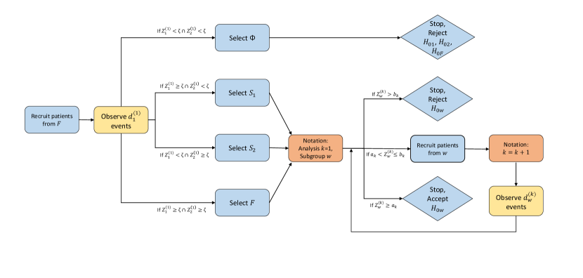
Figure 1: Flow chart for enrichment trial design including number of events observed at each stage.

2.2 The threshold selection rule

We shall use the threshold selection rule to decide which subgroup, if any, to enrich. There are a collection of rules which can be used for selection, for example Chiu et al. (2018) use the maximum test statistic and Burnett and Jennison (2021) present a Bayes optimal rule. The definition of the threshold selection rule is as follows; for some constant $\zeta$, select all groups $j\in\{1,2,F\}$ such that $Z_{j}^{(1)}>\zeta$ (Figure 1). This ensures that only subgroups which have a large enough treatment effect are followed to the second analysis. The threshold selection rule leads to an efficient enrichment trial design because we can find analytical forms for the Type 1 and Type 2 errors and are therefore able to maximise power. A practical advantage is the simplicity of the rule in application. The novel aspect of this work will be to apply this rule in the joint modeling setting.

To calculate $\zeta$, we impose some restrictions which can be customised at the design stage of the trial. First set the configuration of parameters under the global null as $\boldsymbol{\Theta}_{G}:\{\theta_{1}=\theta_{2}=\theta_{F}=0\}$ and the alternative as $\boldsymbol{\Theta}_{A}:\{\theta_{1}=\delta,\theta_{2}=0,\theta_{F}=\lambda\delta\}$. This represents that we believe there is an important effect of treatment in one subgroup $S_{1}$. We require that, under $H_{A}$, it is equally likely to select the full population or no subgroup, and that the subgroup which truly responds well to treatment, is selected a high proportion of times. Let $\mathbb{P}(W=w;\boldsymbol{\Theta}_{A})$ be the probability of selecting subgroup $w\in\{1,2,F,\emptyset\}$ under $H_{A},$ and this value can be calculated by considering the densities of $Z_{1}^{(1)}$ and $Z_{2}^{(1)}$ given by Equation (1). Hence, for some $\psi$, we solve the simultaneous equations $\mathbb{P}\left(W=S_{1};\boldsymbol{\Theta}_{A}\right)=\psi$ and $\mathbb{P}\left(W=F;\boldsymbol{\Theta}_{A}\right)=\mathbb{P}\left(W=\emptyset;\boldsymbol{\Theta}_{A}\right)$. Under this setup, with $\psi=0.6$ and $\delta=-0.5,$ we therefore need $\zeta=0.754$ and $\mathcal{I}^{(1)}_{1}=9.08$.

In order to calculate error rates, we need the joint distribution of the selected test statistic $Z_{W}^{(1)}$ and the population index $W$. For a general configuration of parameters $\boldsymbol{\Theta}$, the joint probability density function is given by

$$f_{Z^{(1)}_{W},W}\left(z^{(1)}_{w},w;\boldsymbol{\Theta}\right)=\mathbb{P}\left(W=w;\boldsymbol{\Theta}\right)f_{Z^{(1)}_{W}|W}\left(z^{(1)}_{w}|W=w;\boldsymbol{\Theta}\right)$$ (2)

where $f_{Z^{(1)}_{W}|W}(z^{(1)}_{w}|W=w;\boldsymbol{\Theta})$ describes the conditional distribution of the test statistic $Z_{W}^{(1)}$ given that subgroup $w$ has been selected, as in Chiu et al. (2018). We now derive explicit forms for the joint densities $f_{Z^{(1)}_{W},W}(z^{(1)}_{w},w;\boldsymbol{\Theta})$ for $w=1,2$ when the threshold rule is used for subgroup selection and in the supplementary materials, we derive $f_{Z^{(1)}_{F},F}(z^{(1)}_{F},F;\boldsymbol{\Theta}).$ At the first interim analysis, the test statistics are such that $Z^{(1)}_{j}\sim N(\theta_{j}(I^{(1)}_{j})^{1/2},1)$ for $j=1,2$ and $Z_{1}^{(1)}$ and $Z_{2}^{(1)}$ are independent. The conditional distribution $f_{Z^{(1)}_{W}|W}(z^{(1)}_{w}|W=w;\boldsymbol{\Theta})$ is given by a truncated normal distribution bounded below by $\zeta$. Hence using Equation (2), we have

$$f_{Z^{(1)}_{1},1}(z^{(1)}_{1},1;\boldsymbol{\Theta})= \Phi\left(\zeta-\theta_{2}\sqrt{\mathcal{I}_{2}^{(1)}}\right)\phi\left(z^{(1)}_{1}-\theta_{1}\sqrt{\mathcal{I}_{1}^{(1)}}\right)$$

$$f_{Z^{(1)}_{2},2}(z^{(1)}_{2},2;\boldsymbol{\Theta})= \Phi\left(\zeta-\theta_{1}\sqrt{\mathcal{I}_{1}^{(1)}}\right)\phi\left(z^{(1)}_{2}-\theta_{2}\sqrt{\mathcal{I}_{2}^{(1)}}\right)$$

$$f_{Z^{(1)}_{F},F}(z^{(1)}_{F},F;\boldsymbol{\Theta})= \frac{\sqrt{\mathcal{I}_{1}^{(1)}\mathcal{I}_{2}^{(1)}}}{\lambda(1-\lambda)\mathcal{I}_{F}^{(1)}}\int_{-\infty}^{\infty}\phi\left(\frac{\sqrt{\mathcal{I}_{1}^{(1)}}(u-\lambda\sqrt{\mathcal{I}_{F}^{(1)}})}{\lambda\sqrt{\mathcal{I}_{F}^{(1)}}}\right)\phi\left(\frac{\sqrt{\mathcal{I}_{2}^{(1)}}(z_{F}^{(1)}-u-(1-\lambda)\sqrt{\mathcal{I}_{F}^{(1)}})}{(1-\lambda)\sqrt{\mathcal{I}_{F}^{(1)}}}\right)du$$

where $\phi(\cdot)$ and $\Phi(\cdot)$ denote the probability density and cummulative distribution functions respectively of a standard normal random variable.

2.3 Calculation of Type 1 error and power

We now consider the possible pathways of the enrichment trial. Then, given the definition of the $Z-$statistics, the threshold selection rule and the joint density function $f_{Z^{(1)}_{F},W}(z^{(1)}_{F},F;\boldsymbol{\Theta}),$ we are equipped to determine error rates for the study. The family wise error rate (FWER), denoted by $\alpha$, is defined as the probability of rejecting one or more null hypotheses $H_{j}$ and power is denoted by $1-\beta$. We shall apply this method in Section 3.2 in order to create an enrichment trial using the joint model for longitudinal and TTE data.

Let $H_{G}$ be the global null hypothesis $\theta_{1}=\theta_{2}=\theta_{F}=0$. There are many pathways which lead to rejecting $H_{G}$. Examples include select $F$ and reject $H_{0,F}$ immediately or select $S_{1}$ then reject $H_{0,1}$ at the second analysis. Considering all options, we have

$$\alpha=\sum_{w\in S}\left\{\int_{b_{1}}^{\infty}f_{Z^{(1)}_{W},W}\left(z^{(1)}_{w},w;\boldsymbol{\Theta}_{G}\right)dz_{w}^{(1)}+\int_{a_{1}}^{b_{1}}\int_{b_{2}}^{\infty}f_{W,2|1}\left(z_{w}^{(2)}|z_{w}^{(1)};\boldsymbol{\Theta}_{G}\right)dz_{w}^{(2)}dz_{w}^{(1)}\right\}.$$ (3)

Here, we have specified that we will only test the hypothesis corresponding to the selected subgroup, since it has the highest chance of being significant. For alternative configurations testing all hypotheses, fixed sequence testing (Westfall and Krishen (2001)) or other alpha propagation methods can be applied.

As in Chiu et al. (2018), we define power as the conditional probability of rejecting $H_{0,1}$ given that subgroup $S_{1}$ is selected. Here, $S_{1}$ can be arbitrarily interchanged for $S_{2}$. This reflects the belief that a “successful" trial is one where the benefitting subgroup is selected and also reports a positive trial outcome. Type 2 error rates are calculated as

$$\beta=\int_{-\infty}^{a_{1}}f_{Z^{(1)}_{W},W}\left(z^{(1)}_{w},w;\boldsymbol{\Theta}_{A}\right)dz_{w}^{(1)}+\int_{a_{1}}^{b_{1}}\int_{-\infty}^{a_{2}}f_{W,2|1}\left(z_{w}^{(2)}|z_{w}^{(1)};\boldsymbol{\Theta}_{A}\right)dz_{w}^{(2)}dz_{w}^{(1)}.$$ (4)

It is now clear that the boundary points $a_{1},a_{2},b_{1}$ and $b_{2}$ can be calculated to satisfy prespecified requirements of FWER $\alpha$ and power $1-\beta$ under $\boldsymbol{\Theta}_{A}$. Further, to ensure that we have four equalities for the four boundary points, we make additional requirements that $\alpha^{(k)}$ is the Type 1 error “spent" and $\beta^{(k)}$ is the Type 2 error spent at analysis $k$ where $\alpha^{(1)}+\alpha^{(2)}=\alpha$ and $\beta^{(1)}+\beta^{(2)}=\beta.$ Then solve

$$\alpha^{(1)} =\sum_{w\in S}\int_{b_{1}}^{\infty}f_{Z^{(1)}_{W},W}\left(z^{(1)}_{w},w;\boldsymbol{\Theta}_{G}\right)dz_{w}^{(1)},\hskip 28.45274pt \beta^{(1)} =\int_{-\infty}^{a_{1}}f_{Z^{(1)}_{W},W}\left(z^{(1)}_{w},w;\boldsymbol{\Theta}_{A}\right)dz_{w}^{(1)}$$

$$\alpha^{(2)} =\sum_{w\in S}\int_{a_{1}}^{b_{1}}\int_{b_{2}}^{\infty}f_{W,2|1}\left(z_{w}^{(2)}|z_{w}^{(1)};\boldsymbol{\Theta}_{G}\right)dz_{w}^{(2)}dz_{w}^{(1)},\hskip 28.45274pt \beta^{(2)} =\int_{a_{1}}^{b_{1}}\int_{-\infty}^{a_{2}}f_{W,2|1}\left(z_{w}^{(2)}|z_{w}^{(1)};\boldsymbol{\Theta}_{A}\right)dz_{w}^{(2)}dz_{w}^{(1)}.$$

The decomposition of the error rates also ensures that the boundary points $a_{1}$ and $b_{1}$ can be calculated at the first analysis before observing the information levels at the second analysis. Hence, there may be the opportunity to stop the trial early without needing to calculate the information levels at the second analysis. This is particularly helpful in trials which use TTE endpoints because the information levels are estimated using the data.

There are many options for the break-down of the error rates. For the models considered, we shall use an error spending design by Gordon Lan and DeMets (1983). In the group sequential setting (without subgroup selection), the error spending test requires specifying the maximum information $\mathcal{I}_{max}$ and then error is spent according to the proportion of information $\mathcal{I}^{(k)}/\mathcal{I}_{max}$ observed at analysis $k$. For the enrichment trial, we propose a similar structure considering $\mathcal{I}_{max}$ to be the maximum information in the full population. Specifically, we shall use the functions $f(t)=\min\{\alpha t^{2},\alpha\}$ and $g(t)=\min\{\beta t^{2},\beta\}$ to determine the amount of error to spend. Then we set $\alpha^{(1)}=f\left(\mathcal{I}_{F}^{(1)}/\mathcal{I}_{max}\right)$, $\alpha^{(2)}=f\left(\mathcal{I}_{F}^{(2)}/\mathcal{I}_{max}\right)-f\left(\mathcal{I}_{F}^{(1)}/\mathcal{I}_{max}\right)$, $\beta^{(1)}=g\left(\mathcal{I}_{F}^{(1)}/\mathcal{I}_{max}\right)$ and $\beta^{(2)}=g\left(\mathcal{I}_{F}^{(2)}/\mathcal{I}_{max}\right)-g\left(\mathcal{I}_{F}^{(1)}/\mathcal{I}_{max}\right)$. We shall discuss the calculation of $\mathcal{I}_{max}$ in the TTE (or joint modeling) setting in Section 2.5.

By construction, the FWER is protected in the weak sense. That is, under $H_{G}:\theta_{1}=\theta_{2}=\theta_{F}=0$ we have FWER $\alpha$ exactly by Equations (3) and (4). We can show that asymptotically we also have strong control of the FWER, which is the probability of rejecting one or more true null hypotheses. We prove this by showing that FWER is maximised under the global null.

Theorem 1.

For global null hypothesis $H_{G}$ and any $\Theta$, we have

$$\limsup\limits_{n\rightarrow\infty}\mathbb{P}(\text{Reject at least one true }H_{j}|\boldsymbol{\Theta})\leq\limsup\limits_{n\rightarrow\infty}\mathbb{P}(\text{reject at least one }H_{j}|H_{G}).$$

Proof.

See the supplementary materials. ∎

2.4 Trials with unpredictable information increments: events based analyses

To complete the calculation of the boundary points $a_{2}$ and $b_{2}$ in Equations (3) and (4), it remains to find the information level at analysis $2$ for the subgroups that have ceased to be observed. That is, suppose that $w\in{1,2,F}$ is the subgroup that has been selected and the trial continues to analysis $2,$ then $\mathcal{I}_{w}^{(2)}$ is observed. However, we also need to know $\mathcal{I}_{j}^{(2)}$ for all $j\neq w$, which is the information that would have been observed if subgroup $j$ were selected.

Many enrichment trial designs focus on the simple example where the outcome measure is normally distributed with known variance. Hence, if the number of patients to be recruited is prespecified, then $\mathcal{I}^{(2)}_{j}$ can be calculated in advance of the trial. However, in trials where the primary endpoint is a TTE variable, information is estimated using the data.

We find that we can accurately forward predict the information levels at future analyses when we know the number of observed events. Hence, instead of prespecifying the number of patients to recruit, we shall presepcify the number of observed events. For subgroup $j=1,2$, let $d_{j}^{(k)}$ be the number of events observed in subgroup $j$ before analysis $k$. We specify that if no early stopping occurs, then the total number of oberved events in the selected subgroup is the same regardless of which subgroup has been selected so that $d^{(2)}_{1}=d^{(2)}_{2}=d^{(2)}_{F}=d^{(2)}$. Figure 1 identifies when the analyses are performed. Note that these values are set as design options and so will be known before commencement of the trial. We shall discuss how to choose these values in Section 2.5.

Further, we relate number of events and information so that we can predict the information level at the second analysis for the unobserved subgroups. Freedman (1982) proves that, in the context of survival analysis, the variance of the log-rank statistic under $H_{G}$ is such that $\mathcal{I}^{(k)}_{j}\approx d^{(k)}_{j}/4$. For analysis methods using test statistics other than the log-rank, we shall extend on this idea and assume that $\mathcal{I}^{(k)}_{j}=d^{(k)}_{j}/m_{j}$ where $m_{j}$ is an arbitrary constant. In the supplementary materials, we show simulation evidence for these relationships. Since each $\mathcal{I}^{(1)}_{j}$ is observed for $j=1,2,F,$ we shall use the proportionality relationship to predict the information at the second analysis for the subgroup which is no longer observed. For $j\neq w$ where $w$ is the subgroup that has been selected at the first interim analysis, we can predict $\mathcal{I}_{j}^{(2)}$ using $\mathcal{I}_{j}^{(2)}=d_{j}^{(1)}d^{(2)}/\mathcal{I}_{j}^{(1)}.$

2.5 Trial design — number of events

We have so far presented the calculation of the boundary points for a trial where the number of events at the interim and final analyses are known prior to commencement. We now discuss the design of the trial, in particular, determining the constants $m_{j}$ and information levels $\mathcal{I}_{j}^{(1)}$ for $j=1,2,F$ and maximum information level $\mathcal{I}_{max}$. These in turn mean that the required numbers of events $d^{(1)}_{j}$ for $j=1,2,F$ and $d^{(2)}$ can be planned. The driving design feature is that we will plan the trial to have power $1-\beta$ under the parameterisation $\boldsymbol{\Theta}_{A}$. We now describe a simulation scheme to determine the constants $m_{j}$ for $j=1,2,F.$

Under the parameterisation $\boldsymbol{\Theta}_{A}$, simulate a data set of $5000$ patients

Let $t_{j,1},\dots,t_{j,n_{j}}$ be the event times in subgroup $j$

for $t_{j,s}=t_{j,1},\dots,t_{j,n_{j}}$ do

     Right-censor all patients at time $t_{j,s}$

     Calculate $\mathcal{I}_{j,s}^{(1)}$ based on data up to time $t_{j,s}$

end for

Fit a linear model, without an intercept term, to the points $(t_{j,1},\mathcal{I}_{j,1}^{(1)}),\dots,(t_{j,n_{j}},\mathcal{I}_{j,n_{j}}^{(1)})$

Use this linear model to estimate the value of $m_{j}$.

It is now possible to calculate the required number of events at the first interim analysis. By Section 2.2, we require $\mathcal{I}_{1}^{(1)}=9.08$ which equates to $d_{1}^{(1)}=9.08m_{1}$ events in subgroup $S_{1}$. Further, we find that $m_{2}=(1-\lambda)m_{1}/\lambda$ and $m_{F}=m_{1}/\lambda$ which equates to $d_{2}^{(1)}=(1-\lambda)d_{1}^{(1)}/\lambda$ and $d_{F}^{(1)}=d_{1}^{(1)}/\lambda$. The design of the trial does not require us to plan $d^{(1)}_{2}$ and $d^{(1)}_{F}$, but this provides us with estimates of the number of events that will be observed at the first analysis. We can also determine the timing of the final analysis at $K=2$. Consider the sequence of information levels given by $(\tilde{\mathcal{I}}^{(1)}_{j},\tilde{\mathcal{I}}^{(2)}_{j})=\left(d_{j}^{(1)}/m_{j},m_{F}\mathcal{I}_{max}/m_{j}\right)$ for $j\in\{1,2,F\}.$ The value of $\mathcal{I}_{max}$ is calculated such that boundary points satisfy $a_{K}=b_{K}$ when the information levels $\tilde{\mathcal{I}}_{j}^{(k)}$ replace $\mathcal{I}_{j}^{(k)}$ in Equations (3) and (4) for $k=1,2$ and $j=1,2,F.$ This is done using an iterative search method. Then, returning to the definition of $\mathcal{I}_{max}$, the total number of events can be found by solving $\mathcal{I}_{F}^{(2)}=\mathcal{I}_{max}$ for $d^{(2)}$.

3 Joint modeling of longitudinal and time-to-event data

3.1 The joint model

The joint model that we consider is an adaptation of Equation (2) of Tsiatis and Davidian (2001) (who shall hereto be referred to as “TD" for short). There are two processes in this model which represent the survival and longitudinal parts separately, and these processes are linked using random effects. Suppose that $Z_{ji}$ is the indicator function that patient $i$ in subgroup $j\in\{1,2,F\}$ receieves the experimental treatment, $X_{ji}(t)$ is the true value of the biomarker at time $t$ and $W_{ji}(t)$ is the observed value of the biomarker. Then the longitudinal model takes the form

$$X_{ji}(t)=b_{0ji}+b_{1ji}t+b_{2j}Z_{ji}t,\hskip 28.45274ptW_{ji}(t)=X_{ji}(t)+\epsilon_{ji}(t)$$ (5)

where $\mathbf{b}_{ji}=(b_{ji0},b_{ji1})$ is a vector of patient specific random effects, $b_{2j}$ is a fixed parameter and $\epsilon_{ji}(t)$ is the measurement error. We make the assumptions that if the longitudinal data for patient $i$ in subgroup $j$ is measured at times $v_{ji1},\dots v_{jim_{ji}}$, then $\epsilon_{ji}(v_{jis})|\mathbf{b}_{ji}\sim N(0,\sigma_{j}^{2})\text{ for }s=1,\dots,m_{ji}$ and $\epsilon_{ji}(v)$ and $\epsilon_{ji}(v^{\prime})$ are independent for $v\neq v^{\prime}.$ This model differs slightly from Equation (2) of TD because of the inclusion of the treatment effect in the longitudinal model. This reflects that longitudinal observations may be affected by treatment. We consider a random effects model where $\mathbf{b}_{j1},\dots,\mathbf{b}_{jn}$ are independent and identically distributed with the following distribution

$$\begin{bmatrix}b_{0ji}\\ b_{1ji}\end{bmatrix}\sim N\left(\begin{bmatrix}\mu_{1j}\\ \mu_{2j}\end{bmatrix},\begin{bmatrix}\phi_{1j}&\phi_{12j}\\ \phi_{12j}&\phi_{2j}\end{bmatrix}\right).$$ (6)

The model for the survival endpoint is a Cox proportional hazards model. Let $\eta_{j}$ be the treatment effect in subgroup $j\in\{1,2,F\}$ and let $\gamma_{j}$ be a scalar coefficient. The baseline hazard function and hazard function for subgroup $j$ are given by

$$h_{0j}(t) =\begin{cases}c_{j}&\text{ if }t\leq 1\\ 5c_{j}/3&\text{ if }t>1\end{cases}$$ (7)

$$h_{ji}(t) =h_{0j}(t)\exp\{\gamma X_{ji}(t)+\eta_{j}Z_{ji}\}$$ (8)

We have chosen to model the baseline hazard function as piecewise constant with a single parameter for simplicity. This is motivated by the dataset, presented in Section 5.1, where we see a sharp difference in the baseline hazard at 1 year. Note that it is the true underlying trajectory $X_{ji}(t)$ which is included as a covariate in the proportional hazards model, whereas the measurements $W_{ji}(t)$ with added error are observed. Here, the coefficients $b_{2j}$ and $\eta_{j}$ both represent treatment effects where $\eta_{j}$ is the direct effect of treatment acting on survival and $b_{2j}$ is the indirect effect. Together, Equations (5)–(7) define the joint model and defines the working model from which we shall perform simulation studies in Section 5.1.

3.2 Conditional score

In the fixed sample setting, TD present the “conditional score" method for fitting the joint model to the data. The method adapts the general theoretical work by Stefanski and Carroll (1987) who find unbiased score functions by conditioning on certain sufficient statistics. The conditional score methodology builds upon the theory of counting processes. The survival counting process is a step function jumping from 0 to 1 at the failure time for an uncensored observation.

We present multi-stage adaptations of some functions presented in TD. Let $t_{ji}^{(k)}$ be the observed event time and let $\delta_{ji}^{(k)}$ be the observed censoring indicator for patient $i$ in subgroup $j\in\{1,2,F\}$ at analysis $k$. This censoring event includes “end of study" censoring for the total follow-up time at each analysis. For the conditional score, to be included in the at-risk set at time $t$ the patient must have at least two longitudinal observations to fit the regression model. At analysis $k$, we define the at-risk process, $Y_{ji}^{(k)}(t)=\mathbb{I}\{t_{ji}^{(k)}\geq t,v_{ji2}\leq t\}$, counting process, $N_{ji}^{(k)}(t)=\mathbb{I}\{t_{ji}^{(k)}\leq t,\delta_{ji}^{(k)}=1,v_{ji2}\leq t\}$ and function $dN_{ji}^{(k)}(t)=\mathbb{I}\{t\leq t_{ji}^{(k)}<t+dt,\delta_{ji}^{(k)}=1,v_{ji2}\leq t\}$ for the joint model.

An object of importance is the sufficient statistic. For patient $i$ in subgroup $j$, let $v_{ji}(u)$ be set of all time points for measurements of the biomarker, up to and including time $u$. Let $\hat{X}_{ji}(u)$ be the ordinary least squares estimate of $X_{ji}(u)$ based on the set of measurements taken at times $v_{ji}(u)$. That is, calculate $\hat{b}_{0ji}(u),\hat{b}_{1ji}(u)$ and $\hat{b}_{j2}(u)$ based on measurements taken at times $v_{ji}(u)$, then $\hat{X}_{ji}(u)=\hat{b}_{0ji}(u)+\hat{b}_{1ji}(u)u+\hat{b}_{j2}(u)Z_{ji}(u)$. As we pass time $v_{jim},$ a new observation $W_{jim}$ is generated and $\hat{X}_{ji}(u)$ is updated. This seems strange since at an early time point, $s$ where $s<u$, we use data $v_{ji}(s)$ in the calculation of $\hat{X}_{ji}(s)$ even though $v_{ji}(u)$ may be available. However, this is necessary for the martingale property to hold for the distributional results of the parameter estimates. Suppose that $\sigma_{j}^{2}\psi_{ji}(u)$ is the variance of $\hat{X}_{ji}(u)$ at time $u$. TD define the sufficient statistic to be the function

$$S_{ji}^{(k)}(t,\gamma_{j},\sigma_{j}^{2})=\hat{b}_{0ji}(t)+\hat{b}_{1ji}(t)t+Z_{ji}\hat{b}_{j2}t+\gamma_{j}\sigma_{j}^{2}\psi_{ji}(t)dN_{ji}^{(k)}(t)$$

which is defined for all $t\in(v_{ji2},t_{ji}^{(k)})$ for patient $i$ in subgroup $j$. Further the multi-stage, dependent on subgroup $j$, version of the quotient function $E_{1}/E_{0}$ in Equation (6) by TD is the $2\times 1$ vector given by

$$E_{j}^{(k)}(u,\gamma_{j},\eta_{j},\sigma_{j}^{2})=\frac{\sum_{i=1}^{n_{j}}\{S_{ji}^{(k)}(u,\gamma_{j},\sigma_{j}^{2}),Z_{ji}\}^{T}\exp\{\gamma S_{ji}^{(k)}(t,\gamma_{j},\sigma_{j}^{2})-\gamma_{j}^{2}\sigma_{j}^{2}\psi_{ji}(t)/2+\eta_{j}Z_{ji}\}Y_{ji}^{(k)}(t)}{\sum_{i=1}^{n_{j}}\exp\{\gamma S_{ji}^{(k)}(t,\gamma_{j},\sigma_{j}^{2})-\gamma_{j}^{2}\sigma_{j}^{2}\psi_{ji}(t)/2+\eta Z_{ji}\}Y_{ji}^{(k)}(t)}.$$

We can now define the conditional score function at analysis $k$ for subgroup $j\in\{1,2,F\}$, denoted $U_{j}^{(k)}(\gamma_{j},\eta_{j},\sigma_{j}^{2})$. Let $\tau_{k}$ be the maximum follow-up time at analysis $k$, then

$$U_{j}^{(k)}(\gamma_{j},\eta_{j},\sigma_{j}^{2})=\int_{0}^{\tau_{k}}\sum_{i=1}^{n_{j}}\left(\{S_{ji}^{(k)}(u,\gamma_{j},\sigma_{j}^{2}),Z_{ji}\}^{T}-E_{j}^{(k)}(u,\gamma_{j},\eta_{j},\sigma_{j}^{2})\right)dN_{ji}^{(k)}(u).$$ (9)

Here, integration over the function $dN_{ji}^{(k)}(u)$ ensures that the integrand is evaluated at the place where $N_{ji}^{(k)}(t)$ jumps from 0 to 1 if $\delta_{ji}^{(k)}=1$ and $v_{ji2}\leq t$, and 0 otherwise. The object $U^{(k)}_{j}(\gamma_{j},\eta_{j},\sigma_{j}^{2})$ has the same dimensionality as $E_{j}^{(k)}(u,\gamma_{j},\eta_{j},\sigma_{j}^{2})$.

Burdon et al. (2022) show that $\mathbb{E}(U_{j}^{(k)}(\gamma_{j},\eta_{j},\sigma_{j}^{2}))=\mathbf{0}$ for each $k=1,\dots,K,$ and $j\in\{1,2,F\}$. Therefore, the conditional score function at analysis $k$ is an estimating function, and set equal to zero defines an estimating equation. Hence, asymptotically normal parameter estimates for $\gamma_{j}$ and $\eta_{j}$ can be found as the root of the estimating equation. As in TD Equation (13), define the pooled estimate $\hat{\sigma}_{j}^{(k)2}=\sum_{i=1}^{n_{j}}\mathbb{I}\{m_{ji}(k)>2\}R_{ji}(k)/\sum_{i=1}^{n_{j}}\mathbb{I}\{m_{ji}(k)>2\}(m_{ji}(k)-2),$ where $R_{ji}(k)$ is the residual sum of squares for the least squares fit to all $m_{ji}(k)$ observations for patient $i$ in subgroup $j$ available at analysis $k$. Then, let $\hat{\gamma}_{j}^{(k)},\hat{\eta}_{j}^{(k)}$ be the values of $\gamma_{j}$ and $\eta_{j}$ respectively such that $U_{j}^{(k)}(\hat{\gamma}_{j}^{(k)},\hat{\eta}_{j}^{(k)},\hat{\sigma}_{j}^{(k)2})=\mathbf{0}.$

We shall use the sandwich estimator, as in Section 2.6 by Wakefield (2013), to calculate a robust estimate for the variance of the treatment effect estimate. Firstly, define matrices $A_{j}^{(k)}=\partial U_{j}^{(k)}(\gamma_{j},\eta_{j},\sigma_{j}^{2})/\partial(\gamma_{j},\eta_{j})^{T}$ and $B_{j}^{(k)}=Var(U^{(k)}_{j}(\gamma_{j},\eta_{j},\sigma_{j}^{2})).$ Burdon et al. (2022) present analytical forms for each of these $2\times 2$ matrices including a detailed calculation for the derivative matrix $A_{j}^{(k)}.$ In practice, $A_{j}^{(k)}$ can be calculated numerically and $B_{j}^{(k)}$ is found by considering the score statistic as a sum over $n_{j}$ patients. Further, these matrices are estimated by substituting the estimates $\hat{\gamma}_{j}^{(k)},\hat{\eta}_{j}^{(k)}$ and $\hat{\sigma}_{j}^{(k)2}$ for $\gamma_{j},\eta_{j}$ and $\sigma_{j}^{2}$ respectively. Then the information for the treatment effect estimate is given by $\mathcal{I}_{j}^{(k)}=n_{j}\left[(A_{j}^{(k)})^{-1}B_{j}^{(k)}((A_{j}^{(k)})^{-1})^{T}\right]^{-1}_{22}.$ The subscript represents that we are interested in the second parameter $\eta_{j}$ in the vector $(\gamma_{j},\eta_{j},\sigma_{j}^{2})^{T}.$

The methodology in Section 2 can now be applied and an enrichment trial performed. The null hypothesis here is $H_{0j}:\eta_{j}\leq 0$ which can be calculated by fnding estimates $\hat{\eta}_{j}^{(k)}$, information levels $\mathcal{I}^{(k)}_{j}$ and $Z$-statistics using the conditional score framework. This is summarised in Table 1. Burdon et al. (2022) show that the $Z$-statistics do not have the canonical joint distribution in Equation (1), however, by proceeding with a group sequential test assuming that this does hold is sensible since Type 1 error rates are conservative and diverge minimally from planned significance level $\alpha$.

It may seem strange that the causal effect of treatment acting through the longitudinal data, $b_{2j},$ is not utilised in the hypothesis test. We have found that we do not lose much power by focusing on the direct effect, $\eta_{j}$. Under sensible choices for the parameter values, the benefits of the conditional score method outweigh the slight increase in power and therefore this will be the method of primary focus. This is a desireable method because the analysis is semi-parametric so that we are not required to specify a distribution for, or estimate, the baseline hazard function $h_{j0}(t).$ Further, we are not required to specify any distributional assumptions for the random effects which makes the conditional score methodology robust to some model misspecifications.

3.3 5-year restricted mean survival time (RMST)

We have presented a joint model for longitudinal and TTE data which includes a causal treatment effect acting through the longitudinal process. So far, we have considered the conditional score method which does not make use of the information about the treatment effect in the longitudinal data. We aim to perform a clinical trial which leverages information on both $\eta_{j}$ and $b_{2j}$ in the joint model. We require a single one dimensional test statistic that summarises the overall effect of treatment and we propose using the restricted mean survival time (RMST) to do so.

Royston and Parmar (2011) define RMST as the area under the survival curve up to time $t^{*}$. The value of $t^{*}$ is fixed at the design stage and we shall discuss our choice. Let $\boldsymbol{\psi}_{j}$ be the $p\times 1$ vector of all parameters in the joint model in subgroup $j$. Suppose that $F_{0j}$ and $F_{1j}$ are time-to-failure random variables for patients on the control and experimental treatment arms respectively and that $S_{0j}(t;\boldsymbol{\psi}_{j})$ and $S_{1j}(t;\boldsymbol{\psi}_{j})$ are the corresponding survival functions integrated over any patient specific random effects. Then the difference in RMST between treatment groups is given by

$$\Delta_{j}(t^{*};\boldsymbol{\psi}_{j})=\mathbb{E}[\min(F_{1j},t^{*})]-\mathbb{E}[\min(F_{0j},t^{*})]=\int_{0}^{t^{*}}\left[S_{1j}(t;\boldsymbol{\psi}_{j})-S_{0j}(t;\boldsymbol{\psi}_{j})\right]dt.$$ (10)

Most commonly, non-parametric methods are employed for estimating $\Delta_{j}(t^{*};\boldsymbol{\psi}_{j})$, which include integration under the Kaplan-Meier curve and bootstrap methods to estimate the variance. Lu and Tian (2020) consider some practical design challenges for such methods. Non-parametric estimation is a popular solution when the proportional hazards assumption does not hold since the estimator is robust to model misspecification. Our motivation for using RMST is to find a test statistic summarising the effect of two treatment effect parameters and we wish to exploit the gain in power accrued from covariate information. Hence we shall focus on the parameteric estimator.

We now present the exact analytical form for the difference in RMST for the joint model Equations (5)–(7). The cummulative hazard function for patient $i$ in subgroup $j$ is given in two parts.

$$\text{For }t\leq 1:H_{ji}(t;\boldsymbol{\psi}_{j})= \frac{c_{j}\exp\{\gamma_{j}b_{0ji}+\eta_{j}Z_{ji}\}}{\gamma_{j}(b_{1ji}+b_{2j}Z_{ji})}[\exp\{\gamma_{j}t(b_{1ji}+b_{2j}Z_{ji})\}-1]$$

$$\text{For }t>1:H_{ji}(t;\boldsymbol{\psi}_{j})= \frac{\exp\{\gamma_{j}b_{0ji}+\eta_{j}Z_{ji}\}}{\gamma_{j}(b_{1ji}+b_{2j}Z_{ji})}[0.4c_{j}\exp\{\gamma_{j}(b_{1ji}+b_{2j}Z_{ji})\}+0.6c_{j}\exp\{\gamma_{j}t(b_{1ji}+b_{2j}Z_{ji})\}-1].$$

The control and experimental treatment survival functions integrated over the random effects are

$$S_{0j}(t;\boldsymbol{\psi}_{j}) =\int_{-\infty}^{\infty}\exp\{-H_{ji}(t;\boldsymbol{\psi}_{j},Z_{ji}=0\}f(b_{0ji},b_{1ji})db_{0ji}db_{1ji}$$

$$S_{1j}(t;\boldsymbol{\psi}_{j}) =\int_{-\infty}^{\infty}\exp\{-H_{ji}(t;\boldsymbol{\psi}_{j},Z_{ji}=1\}f(b_{0ji},b_{1ji})db_{0ji}db_{1ji}$$

where $f(b_{0ji},b_{1ji})$ is the probability density function for the normal distribution given in Equation (6). Gauss-Hermite integration can be used to efficiently calculate the integrals over $b_{0ji}$ and $b_{1ji}$. The survival functions are then substituted into Equation (10) to calculate $\Delta_{j}(t^{*};\boldsymbol{\psi}_{j}).$

The parametric RMST estimate can be found by substituting the maximum likelihood estimate (MLE) for the vector of model parameters into the model-based definition of RMST. Rizopoulos (2012) presents the full likelihood function for the joint model from which we can obtain the MLE $\hat{\boldsymbol{\psi}}^{(k)}_{j}$ at analysis $k.$ An estimate for the treatment difference is given by $\Delta_{j}(t^{*};\hat{\boldsymbol{\psi}}_{j}^{(k)})$ for $k=1,\dots,K.$

The delta method, as in Doob (1935), can be used calculate the variance of the parametric RMST estimate. We have that $\hat{\boldsymbol{\psi}}^{(k)}_{j}$ has the same dimensionality as $\boldsymbol{\psi}_{j}$, a $p\times 1$ vector. Let $\Sigma_{j}^{(k)}$ be the $p\times p$ covariance matrix of the MLE $\hat{\boldsymbol{\psi}}_{j}^{(k)}$ at analysis $k$, then we have that $n^{1/2}(\hat{\boldsymbol{\psi}}_{j}^{(k)}-\boldsymbol{\psi}_{j})\xrightarrow{d}N(\mathbf{0},\Sigma_{j}^{(k)})$. The information level at analysis $k$ for the difference in RMST between treatment arms is given by $\mathcal{I}^{(k)}_{j}=n_{j}\left(\left[\partial\Delta_{j}(t^{*};\hat{\boldsymbol{\psi}}_{j}^{(k)})/\partial\boldsymbol{\psi}_{j}\right]^{T}\Sigma_{j}^{(k)}\left[\partial\Delta_{j}(t^{*};\hat{\boldsymbol{\psi}}_{j}^{(k)})/\partial\boldsymbol{\psi}_{j}\right]\right)^{-1}$ where $\partial\Delta_{j}(t^{*};\hat{\boldsymbol{\psi}}_{j}^{(k)})/\partial\boldsymbol{\psi}_{j}$ is the $p\times 1$ vector which is the first derivative of the function $\Delta_{j}(t^{*};\boldsymbol{\psi}_{j})$ with respect to the vector $\boldsymbol{\psi}_{j}$ evaluated at $\hat{\boldsymbol{\psi}}_{j}^{(k)}$. In the calculation of $\mathcal{I}_{j}^{(k)},$ a consistent estimate $\hat{\Sigma}_{j}^{(k)}$ can be substituted in place of the covariance matrix $\Sigma_{j}^{(k)}$. In practice, the MLE $\hat{\boldsymbol{\psi}}^{(k)}_{j}$ and an estimate of the covariance matrix can be calculated using the R package JM by Rizopoulos (2012).

In a later paper, Royston and Parmar (2013) extend on their earlier work and give particular emphasis on the choice of truncation time $t^{*}$. The authors suggest taking $t^{*}$ as the value that minimises the expected sample size given the recruitment time and minimum follow-up time. We find that for all parameter values considered in Section 5.2, the required sample size reduces with $t^{*}$. Further, we shall see that each trial has recruitment roughly 2 years and final analysis time at roughly 5 years, although these analysis times are events based so cannot be known exactly. To ensure that the method is robust to model misspecifications, it is important to avoid extrapolation of the RMST estimate beyone analysis time. Hence, we have chosen to use $t^{*}=5.$

To summarise the overall effect of treatment on survival, which incorporates both treatment effects $b_{2j}$ and $\eta_{j},$ we test the null hypothesis $H_{0j}:\Delta_{j}(5;\boldsymbol{\psi}_{j})\leq 0$. To do so, we define RMST estimates $\Delta_{j}(5;\hat{\boldsymbol{\psi}}_{j}^{(k)}),$ information levels $\mathcal{I}_{j}^{(k)}$ and $Z$-statistics for each $k=1,\dots,K$ and $j=1,2,F.$ This is summarised in Table 1. We see in Section 5.2 that under some scenarios, this method is more powerful than the conditional score method.

4 Alternative models and their analysis methods

4.1 Cox proportional hazards model

Methods which leverage information from biomarkers in TTE studies are yet to be established. The current best practice for adaptive designs with a TTE endpoint is to base analyses on Cox proportional hazards models. We emulate this conventionality in order to assess the gain in power from including the longitudinal data in the analysis. To do so, we shall present a simple Cox proportional hazards model and define a hypothesis test that can be used in accordance with the threshold selection rule to perform an enrichment trial.

Denote $\tilde{h}_{0j}(t)$ as the baseline hazard function, $\tilde{\eta}_{j}$ the treatment effect and $Z_{ji}$ as the treatment indicator that patient $i$ in subgroup $j\in\{1,2,F\}$ receives the new treatment. Then the hazard function for the survival model is given by

$$h_{ji}(t)=\tilde{h}_{0j}(t)\exp\{\tilde{\eta}_{j}Z_{ji}\}.$$ (11)

We note the similarities in definition between $\tilde{h}_{0j}(t)$ and $h_{0j}(t)$ of Section 3.1 and also $\tilde{\eta}_{j}$ and $\eta_{j}$, however these objects are not exactly the same since they arise from different models. This highlights the fact that when the joint model is true, but we fit the data to the Cox proportional hazards model, then this will be a misspecified model and vice versa.

Similarly to Section 3.2, at analysis $k$, we define the at-risk and counting processes. With the same definitions for the observed event time $t_{ji}^{(k)}$ and censoring indicator, $\delta_{ji}^{(k)}$, these are $\tilde{Y}_{ji}^{(k)}(t)=\mathbb{I}\{t_{ji}^{(k)}\geq t\}$ and $d\tilde{N}_{ji}^{(k)}(t)=\mathbb{I}\{t\leq t_{ji}^{(k)}<t+dt,\delta_{ji}^{(k)}=1\}.$ As in Jennison and Turnbull (1997), the function $\tilde{E}_{j}^{(k)}(u,\tilde{\eta}_{j})$ and the score function $\tilde{U}_{j}^{(k)}(\tilde{\eta}_{j})$ at analysis $k$ are given by

$$\tilde{E}_{j}^{(k)}(u,\tilde{\eta}_{j})=\frac{\sum_{i=1}^{n_{j}}Z_{ji}\exp\{\tilde{\eta}_{j}Z_{ji}\}\tilde{Y}_{ji}^{(k)}(t)}{\sum_{i=1}^{n_{j}}\exp\{\tilde{\eta}_{j}Z_{ji}\}\tilde{Y}_{ji}^{(k)}(t)},\hskip 28.45274pt\tilde{U}_{j}^{(k)}(\tilde{\eta}_{j})=\int_{0}^{\tau_{k}}\sum_{i=1}^{n_{j}}\left(Z_{ji}-\tilde{E}_{j}^{(k)}(u,\tilde{\eta}_{j})\right)d\tilde{N}_{ji}^{(k)}(u).$$ (12)

The function $\tilde{U}_{j}^{(k)}(\cdot)$ is a score function and $\tilde{\eta}_{j}$ can be estimated by solving the equation $\tilde{U}_{j}^{(k)}(\tilde{\eta}_{j})=0$ for $\tilde{\eta}_{j}$. Let this estimate, at analysis $k$, be denoted by $\hat{\eta}_{j}^{(k)}$. By standard results by Jennison and Turnbull (1997), the estimates $\hat{\eta}_{j}^{(k)}$ follow the CJD where the information level at analysis $k$ is given by $\mathcal{I}^{(k)}_{j}=n_{j}\left[\partial\tilde{U}^{(k)}_{j}(\hat{\eta}_{j}^{(k)})/\partial\tilde{\eta}_{j}\right]^{-1}.$

In Equation (11), the parameter $\tilde{\eta}_{j}$ describes the entire effect of treatment on survival. Hence, when analysing data using this model, a suitable null hypothesis is given by $H_{0j}:\tilde{\eta}_{j}\leq 0$ and this can be tested at analysis $k=1,\dots,K$ by calculating a treatment effect estimate $\hat{\eta}_{j}^{(k)}$, information level $\mathcal{I}_{j}^{(k)}$ and $Z$-statistic. The resultsing $Z$-statistics have the CJD given in Equation (1) and the mothodology of Sections 2 can be used to create an enrichment trial design.

Some advantages of this simplified Cox proportional hazards model are that we need not specify the baseline hazard function since the maximum partial likelihood analysis is semiparametric and requires no assumptions regarding $\tilde{h}_{0j}(t).$ Further, there is no criteria to have a minimum of two longitudinal observations to be included in the at-risk process.

4.2 Cox proportional hazards model with longitudinal data as a time-varying covariate

A final option for analysis is one where the longitudinal data is included but is assumed to be free of measurement error. This requires a more sophisticated model than the simple Cox proportional hazards model of Section 4.1 and represents a trial where the longitudinal data is regarded as important enough to be considered and included. However, this is still a naive approach since the model will be misspecified in the presence of measurement error. For the purpose of assessing the necessity of correctly modeling the data, we shall fit a Cox proportional hazards model to the data where the longitudinal data is treated as a time-varying covariate.

In what follows, the definitions of the treatment indicator $Z_{ji}$ and longitudinal data measurements $W_{ji}(v_{ji1}),\dots,W_{ji}(v_{jim_{ji}})$ remain the same as in Section 3.1 and the at-risk process $\tilde{Y}_{ji}^{(k)}(t)$ and counting process function $d\tilde{N}_{ji}^{(k)}(u)$ are as in Section 4.1. Let $\dot{\gamma}_{j}$ and $\dot{\eta}_{j}$ be longitudinal data and treatment coefficients respectively, then the hazard function is given by

$$h_{ji}(t)=\dot{h}_{j0}(t)\exp\{\dot{\gamma}_{j}W_{ji}(t)+\dot{\eta}_{j}Z_{ji}\}.$$ (13)

This model differs from the joint model because the assumption here is that $W_{ji}(t)$ is a function of time that is measured without error. In reality we often have measurments $W_{ji}(v_{ji1}),\dots,W_{i}(v_{jim_{ji}})$ for patient $i$ in subgroup $j$ that include noise around a true underlying trajectory.

The function $\dot{E}^{(k)}_{j}(u,\cdot)$ and score statistic $\dot{U}^{(k)}_{j}(\cdot)$ for this model are given by

$$\dot{E}^{(k)}_{j}(u,\dot{\eta}_{j}) =\frac{\sum_{i=1}^{n_{j}}\{W_{ji}(t),Z_{ji}\}^{T}\exp\{\dot{\gamma}_{j}W_{ji}(t)+\dot{\eta}_{j}Z_{ji}\}\tilde{Y}_{ji}^{(k)}(t)}{\sum_{i=1}^{n_{j}}\exp\{\dot{\gamma}_{j}W_{ji}(t)+\dot{\eta}_{j}Z_{ji}\}\tilde{Y}_{ji}^{(k)}(t)}$$

$$\dot{U}^{(k)}_{j}(\dot{\eta}_{j}) =\int_{0}^{\tau_{k}}\sum_{i=1}^{n_{j}}\left(\{W_{ji}(t),Z_{ji}\}^{T}-\dot{E}^{(k)}_{j}(u,\dot{\eta}_{j})\right)d\tilde{N}_{ji}^{(k)}(u).$$ (14)

Both objects $\dot{E}^{(k)}_{j}(u,\dot{\eta}_{j})$ and $\dot{U}^{(k)}_{j}(\dot{\eta}_{j})$ are $2\times 1$ dimensional vectors. To evaluate these objects, we will need to know $W_{ji}(t_{js})$ which is the value of the time-varying covariate for patient $i$ in subgroup $j$, evaluated at the event time of patient $s$ in subgroup $j$. For this model, $W_{ji}(\cdot)$ is a function of time and is known. For calculation purposes, for $t>v$, we shall set $W_{ji}(t)$ as $W_{ji}(v)$ where $v=max(v_{jim}|v_{jim}\leq t)$.

In a similar manner to Section 4.1, and summarised in Table 1, a suitable hytpothesis test based on this model is $H_{0j}:\dot{\eta}_{j}\leq 0.$ This can be tested by finding $Z-$statistics, with the CJD of Equation (1) and following the enrichment trial design of Section 2. These test statistics are calculated as $Z^{(k)}_{j}=\hat{\eta}^{(k)}_{j}\sqrt{\mathcal{I}^{(k)}_{j}}$ where $\hat{\eta}_{j}^{(k)}$ is the value of $\dot{\eta}_{j}$ such that $\dot{U}^{(k)}_{j}(\dot{\eta}_{j})=0$ and the information level is given by $\mathcal{I}^{(k)}_{j}=n_{j}\left[\partial\tilde{U}^{(k)}_{j}(\hat{\eta}_{j}^{(k)})/\partial\dot{\eta}_{j}\right]^{-1}.$

Again, this analysis method is semiparametric so that the baseline hazard function does not need to be estimated. Further, this model includes the longitudinal data however there are no distribution assumptions about the random effects $\mathbf{b}_{j1},\dots,\mathbf{b}_{jn_{j}}$. In fact, under this model, we need not specify the structure of the trajectory of the longitudinal data.

5 Results

5.1 Example: A clinical trial for the treatment of metastatic breast cancer

We shall apply the joint modeling methodology to a study by Dawson et al. (2013) which was designed to compare different biomarkers and their accuracy in monitoring tumour burden among women with metastatic breast cancer. The investigators found that circulating tumour DNA (ctDNA) was successfully detected and highly correlated with OS. As a posthoc analysis, survival curves were estimated under different quantiles of ctDNA, however this study could benefit from joint modeling analyses. Further, the HER2 status of each patient was presented and we shall define $S_{1}$ and $S_{2}$ as the subgroups of women whose HER2 status are negative and positive respectively. The prevalence of HER2 negative patients is found to be $\lambda=2/3$ in this dataset which is in accordance with pivotal results of Slamon et al. (1987) who showed that HER2 status is highly correlated with OS. The authors stress that patients who are HER2 positive may be resistant to conventional therapies which confirms the suitability of the assumption under $H_{A}$ that only patients in subgroup $S_{1}$ will benefit from the experimental treatment.

For the presented analyses, we shall assume that the true model is the joint model. Hence, the working model for data generation is given by Equations (5)–(7) and parameter values for simulation studies are informed using the metastatic breast cancer dataset. We removed patients whose ER status is negative, to retain 27 patients and following Barnett et al. (2021), measurements of ctDNA which were "not detected" were set to 1.5 (Copies/ml). The resulting dataset contains multiple treatment arms and dosing schedules, hence, we fit the model under the assumption that this dataset represents standard of care (control group). The parameter values, which shall remain fixed throughout the simulation studies are given by

$$\lambda=1/3,\gamma=\gamma_{1}=\gamma_{2}=0.8,(\phi_{1},\phi_{12},\phi_{2})=(\phi_{11},\phi_{121},\phi_{21})=(\phi_{12},\phi_{122},\phi_{22})=(2.5,1.7,5),$$

$$\sigma^{2}=\sigma_{1}^{2}=\sigma_{2}^{2}=1,(\mu_{01},\mu_{11})=(\mu_{02},\mu_{12})=(4.23,1.81),c_{1}=c_{2}=0.0085.$$ (15)

Remaining parameters which are needed to fully define $\boldsymbol{\Theta}_{0}$ and $\boldsymbol{\Theta}_{A}$ include $\eta_{j}$ and $b_{2j}$ for each $j=1,2,F.$ To represent no differences between control and treated groups under $H_{0j}$, let $\eta_{j}=b_{2j}=0$ for each $j=1,2,F$. Then, as in Section 2.2, we expect HER2 negative patients to respond well to treatment and HER positive patients be unaffected by tretament which is given by $H_{A1}:\eta_{1}=-0.5,b_{21}=-0.5$ and $H_{A2}:\eta_{2}=b_{22}=0.$

In what follows, ctDNA measurements will be observed, via a blood test, at two weeks for the first three months following entry to study and then once per month. The necessity of performing regular blood tests may be considered a draw-back of including the longitudinal data in the analysis method. We present the number of hospital visits per patient in the supplementay materials. The final object of importance which is required for data genration is the mechanism which simulates censoring times, $y_{1},\dots,y_{n}$. We shall simulate these according to the distribution $y_{i}\sim Exp(5\times 10^{-5})$ and this is independent of the time-to-event outcome to reflect noninformative censoring. This results in roughly $10\%$ of patients being lost to follow-up.

5.2 Efficiency comparison

The purpose of this comparison is to assess the gain by including the longitudinal data and to decide whether correctly modeling the measurement error is necessary. We shall focus on power as a measure of efficiency between the different methods and we compare some other outcome measures, such as number of hospital visits and expected stopping time in the supplementary materials. The four analysis methods are summarised in Table 1. This includes the hypothesis that is being tested and a summary desciption of how to calculate test statistics $\hat{\theta}^{(k)}_{j}$ and information levels $\mathcal{I}^{(k)}$ for subgroup $j\in\{1,2,F\}$ at analysis $k.$

Table 1: Null hypothesis, treatment effect estimate and information for each analysis method.

Analysis method	$H_{0j}$	$\hat{\theta}^{(k)}_{j}$	$\mathcal{I}_{j}^{(k)}$
Conditional score	$\eta_{j}=0$	The value of $\eta_{j}$ such that	$n_{j}\left[(A_{j}^{(k)})^{-1}B_{j}^{(k)}((A_{j}^{(k)})^{-1})^{T}\right]^{-1}_{22}$
		$U_{j}^{(k)}(\gamma_{j},\eta_{j},\sigma_{j}^{2})=0$	where
			$A_{j}^{(k)}=\frac{\partial}{\partial(\gamma_{j},\eta_{j})^{T}}U^{(k)}_{j}(\gamma_{j},\eta_{j},\sigma_{j}^{2})$
			$B_{j}^{(k)}=Var(U_{j}^{(k)}(\gamma_{j},\eta_{j},\sigma_{j}^{2}))$
RMST	$\Delta_{j}(5;\boldsymbol{\psi}_{j})=0$	$\Delta_{j}(5;\hat{\boldsymbol{\psi}}^{(k)}_{j})$ where	$n_{j}\left(\left[\frac{\partial\Delta_{j}(5;\boldsymbol{\psi}_{j})}{\partial\boldsymbol{\psi}_{j}}\bigg{|}_{\boldsymbol{\psi}_{j}=\hat{\boldsymbol{\psi}}_{j}^{(k)}}\right]^{T}\Sigma_{j}^{(k)}\left[\frac{\partial\Delta_{j}(5;\boldsymbol{\psi}_{j})}{\partial\boldsymbol{\psi}_{j}}\bigg{|}_{\boldsymbol{\psi}_{j}=\hat{\boldsymbol{\psi}}_{j}^{(k)}}\right]\right)^{-1}$
		$\hat{\boldsymbol{\psi}^{(k)}_{j}}$ is MLE
Cox model	$\tilde{\eta}_{j}=0$	The value of $\tilde{\eta}_{j}$ such that	$n_{j}\left[\frac{\partial}{\partial\tilde{\eta}_{j}}\tilde{U}^{(k)}_{j}(\tilde{\eta}_{j})\bigg{|}_{\tilde{\eta}_{j}=\hat{\eta}_{j}^{(k)}}\right]^{-1}$
		$\tilde{U}^{(k)}(\gamma_{j},\tilde{\eta}_{j},\sigma_{j}^{2})=0$
Cox model with	$\dot{\eta}_{j}=0$	The value of $\dot{\eta}_{j}$ such that	$n_{j}\left[\frac{\partial}{\partial\dot{\eta}_{j}}\tilde{U}^{(k)}_{j}(\dot{\eta}_{j})\bigg{|}_{\dot{\eta}_{j}=\hat{\eta}_{j}^{(k)}}\right]^{-1}$
biomarker		$\dot{U}^{(k)}(\gamma_{j},\dot{\eta}_{j},\sigma_{j}^{2})=0$

The number of events at the first analysis in subgroup $S_{1}$, denoted $d^{(1)}_{1}$, have been chosen to ensure that subgroup $S_{1}$ is selected rougly $60\%$ of the time, using the conditional score method, and the total number of events at the second analysis, $d^{(2)},$ have been chosen to attain power of $90\%$ as described in Section 2.5. These numbers of events are displayed in Table 2 for a range of values of $\gamma,\sigma^{2}$ and $\phi_{2}$. As $\gamma$ increases, we see that both the required $d^{(1)}_{1}$ and $d^{(2)}$ increase. When $\gamma=1.2$ and with a small number of events at the first interim analysis, it is not always possible to find a root to Equation (9). The consequence is that the required $d^{(1)}_{1}$ and $d^{(2)}$ are high to ensure that large sample properties of the estimator hold. We have not seen this problem occur for $\gamma\leq 0.8.$ Similarly, the required number of events increase with $\sigma.$ That is, as the longitudinal data becomes more noisey, more events and hence more information is needed to achieve power and selection probabilities. The values of $d_{1}^{(1)}$ and $d^{(2)}$ are immune to changes in $\phi_{2}$, which represents the degree of similarity between patients’ longitudinal trajectories.

Table 2: Design parameters.

$\boldsymbol{\phi}$	$\boldsymbol{\sigma}$	$(d^{(1)}_{1},d^{(2)})$
		$\boldsymbol{\gamma}\mathbf{=0}$	$\boldsymbol{\gamma}\mathbf{=0.4}$	$\boldsymbol{\gamma}\mathbf{=0.8}$	$\boldsymbol{\gamma}\mathbf{=1.2}$
$\mathbf{5}$	$\mathbf{0}$	(41,180)	(40,170)	(42,170)	(44,175)
$\mathbf{5}$	$\mathbf{0.5}$	(41,178)	(41,165)	(43,175)	(48,190)
$\mathbf{5}$	$\mathbf{1}$	(41,170)	(42,180)	(49,215)	(62,271)
$\mathbf{5}$	$\mathbf{1.5}$	(44,195)	(49,190)	(60,250)	(80,350)
$\mathbf{0}$	$\mathbf{1}$	(41,160)	(40,175)	(42,200)	(61,266)
$\mathbf{2.5}$	$\mathbf{1}$	(41,165)	(42,178)	(50,195)	(69,302)
$\mathbf{5}$	$\mathbf{1}$	(41,170)	(42,180)	(49,215)	(62,271)
$\mathbf{7.5}$	$\mathbf{1}$	(41,180)	(45,190)	(50,200)	(70,300)

We now put the enrichment methodology into practice using simulation studies. For one simulation; generate a dataset of patients from the joint model, then subgroup selection and decisions about $H_{0}$ are performed after $d_{1}^{(1)}$ and $d^{(2)}$ events have been observed according to Table 2. All four methods in the summary Table 1 are performed on the same dataset and after the same number of events. This is so that differences in the trial results can be attributed to the analysis methodology and not trial design features. The simulations are repeated $N=10^{4}$ times for each set of parameter values and then power is caluclated as the proportion of simulations which select subgroup $S_{1}$ and reject $H_{01}$ as described in Section 2.3.

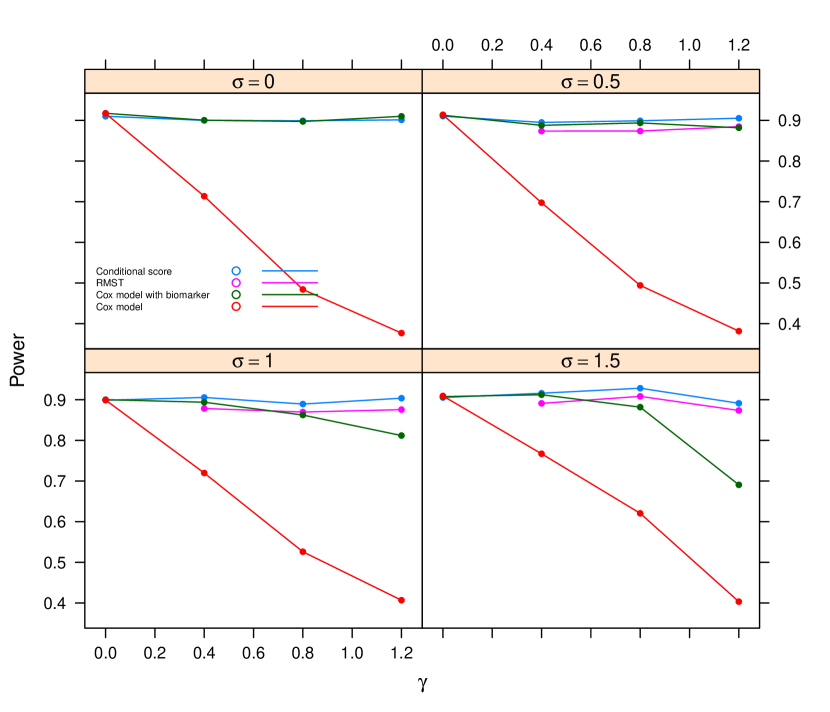
Figure 2: Power results for a study with $10^{4}$ simulations displaying changes in parameters $\gamma$ and $\sigma$. All other parameters are as in (15).

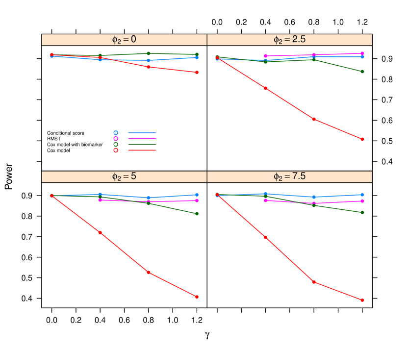
Figure 3: Power results for a study with $10^{4}$ simulations displaying changes in parameters $\gamma$ and $\phi_{2}$. All other parameters are as in (15).

Figures 2 and 3 show the power comparison between the different methods and how power is affected by the parameters $\gamma,\sigma^{2}$ and $\phi_{2}$. The numeric values in these figures are presented in the supplementary materials. It is clear that the conditional score method is most efficient since power is highest across nearly all parameter combinations. When $\gamma=0$, the conditional score method may suffer from a small loss in power in comparison to other methods. This is the case where longitudinal data has no impact on the survival outcome so including it in the analysis is futile. For $\gamma\neq 0$ however, a gain in power between 0.18 to 0.52 is seen.

The RMST methodology is efficient in the sense that power is close to the conditional score method in all cases. This method relies on finding maximum likelihood estimates and the model is overparameterised when any parameter is equal to zero. In such a case, the resulting covariance matrix is often not positive semi-definite and the analysis cannot be performed. This is the reason for missing entries in Figures 2 and 3. This method appears to have higher power for $\phi_{2}=2.5$ however in the supplementary materials, we show that the probability of selecting $S_{1}$ is low in this case and hence power is subjected to higher uncertainty. This method allows us to make inferences which leverage information about the treatment effect in the longitudinal data, however there is not much power to be gained by doing so. Additional model assumptions, such as the distribution of the random effects $\mathbf{b}_{j1},\dots,\mathbf{b}_{jn_{j}}$ and the functional form of the baseline hazard function $h_{0j}(t)$ are required for this method to be used. Further, there is another complication relating to the choice of the truncation time $t^{*}$.

Fitting the data to the simple Cox model is very inefficient and in the extreme cases, power is below $0.4.$ The sample size that would be needed to increase power to 0.9 in such a scenario is excessive. Figure 2 shows that this simple method has power lower than the conditional score method whenever $\gamma\neq 0$ and becomes increasingly inefficient as $\gamma$ increases and also shows that the efficiency of this method is not affected by $\sigma.$ Figure 3 suggests that power might decrease with $\phi_{2}$. Hence, it is important to include the longitudinal data in the analysis when there is a suspected correlation between the longitudinal data and the survival endpoint.

The final method, where TTE outcomes are fit to a Cox proportional hazards model with the longitudinal data as a time-varying covariate, appears to be a simple yet effective way of including longitudinal data in the analysis. The achieved power is at least 0.69 but is usually lower than the conditional score method. However, scenarios where this method outperformes the conditional score are when $\sigma=0$ or $\phi_{2}=0$ indicating that the longitudinal data is free of measurement error or there are no between-patient differences between the slopes of the longitudinal trajectories. The efficiency decreases as longitudinal data increase in noise or as patient differences become larger, that is as $\sigma$ and $\phi_{2}$ increase. This method has the advantage that we do not need to specify the functional form of the longitudinal data, for example that it is linear in time. Taking these advantages into account, we still believe that the most efficient and practical method is the conditional score, which includes the longitudinal data and takes into account the measurement error.

6 Discussion

In current oncology practice and cancer clinical trials, the efficient testing of novel therapies is crucial to focus these on the patient subgroups most likely to benefit. Too many patients receive treatments that either do not work particularly well, are toxic, or sometimes even both.

We have shown that the threshold selection rule can be combined with an error spending boundary to create an efficient enrichment trial. This is potentially suitable for any trial where the primary outcome is a TTE variable and we present a method to establish the required number of events at the design stage of the trial. The novel aspect of this work is that these methods can be applied to an endpoint which is the treatment effect in a joint model for longitudinal and TTE data. By including these routinely collected biomarker outcomes in the analysis to leverage this additional information, the enrichment trial has higher power compared to the enrichment trial where the longitudinal data is left out of the analysis. Bauer et al. (2010) show that bias is prevalent in designs with selection. In our case, selection bias occurs as the treatment effect estimate in the selected subgroup is inflated in later analyses which could affect the trial results. However, unlike most other selection schemes, the threshold selection rule adjusts for the magnitude of the treatment effect at the design stage so another advantage is that selection bias is incorporated into the decision making process.

Further, we compared this joint modeling approach with a model which used the longitudinal data but naively assumed this was free of measurement error. Again, the joint model performed more effectively in most cases. This naive approach was slightly more efficient when the longitudinal data was truly free from measurement error, there was no correlation between the two endpoints or there was no heterogeneity between patients’ biomarker trajectories. However, we believe that these situations are rare in practice and the gain in power from joint modeling outweighs this downside.

Software

All statistical computing and analyses were performed using the software environment R version 4.0.2. Software relating to the examples in this paper is available at https://github.com/abigailburdon/Adaptive-enrichment-with-joint-models.

References

- Barnett et al. [2021] Helen Yvette Barnett, Helena Geys, Tom Jacobs, and Thomas Jaki. Methods for non-compartmental pharmacokinetic analysis with observations below the limit of quantification. Statistics in Biopharmaceutical Research, 13(1):59–70, 2021.
- Bauer et al. [2010] Peter Bauer, Franz Koenig, Werner Brannath, and Martin Posch. Selection and bias—two hostile brothers. Statistics in medicine, 29(1):1–13, 2010.
- Burdon et al. [2022] Abigail J. Burdon, Lisa V. Hampson, and Christopher Jennison. Joint modelling of longitudinal and time-to-event data applied to group sequential clinical trials. https://doi.org/10.48550/arxiv.2211.16138, 2022. URL https://arxiv.org/abs/2211.16138.
- Burnett and Jennison [2021] Thomas Burnett and Christopher Jennison. Adaptive enrichment trials: What are the benefits? Statistics in medicine, 40(3):690–711, 2021.
- Burnett et al. [2020] Thomas Burnett, Pavel Mozgunov, Philip Pallmann, Sofia S Villar, Graham M Wheeler, and Thomas Jaki. Adding flexibility to clinical trial designs: an example-based guide to the practical use of adaptive designs. BMC medicine, 18(1):1–21, 2020.
- Chiu et al. [2018] Yi-Da Chiu, Franz Koenig, Martin Posch, and Thomas Jaki. Design and estimation in clinical trials with subpopulation selection. Statistics in medicine, 37(29):4335–4352, 2018.
- Dawson et al. [2013] Sarah-Jane Dawson, Dana WY Tsui, Muhammed Murtaza, Heather Biggs, Oscar M Rueda, Suet-Feung Chin, Mark J Dunning, Davina Gale, Tim Forshew, Betania Mahler-Araujo, et al. Analysis of circulating tumor dna to monitor metastatic breast cancer. New England Journal of Medicine, 368(13):1199–1209, 2013.
- Doob [1935] Joseph L Doob. The limiting distributions of certain statistics. The Annals of Mathematical Statistics, 6(3):160–169, 1935.
- Freedman [1982] Laurence S Freedman. Tables of the number of patients required in clinical trials using the logrank test. Statistics in medicine, 1(2):121–129, 1982.
- Gordon Lan and DeMets [1983] KK Gordon Lan and David L DeMets. Discrete sequential boundaries for clinical trials. Biometrika, 70(3):659–663, 1983.
- Jennison and Turnbull [1997] Christopher Jennison and Bruce W Turnbull. Group-sequential analysis incorporating covariate information. Journal of the American Statistical Association, 92(440):1330–1341, 1997.
- Jennison and Turnbull [2000] Christopher Jennison and Bruce W Turnbull. Group Sequential Methods with Applications to Clinical Trials. London: Chapman and Hall/CRC, 2000.
- Lu and Tian [2020] Ying Lu and Lu Tian. Statistical considerations for sequential analysis of the restricted mean survival time for randomized clinical trials. Statistics in Biopharmaceutical Research, pages 1–9, 2020.
- Magnusson and Turnbull [2013] Baldur P Magnusson and Bruce W Turnbull. Group sequential enrichment design incorporating subgroup selection. Statistics in medicine, 32(16):2695–2714, 2013.
- Ondra et al. [2016] Thomas Ondra, Alex Dmitrienko, Tim Friede, Alexandra Graf, Frank Miller, Nigel Stallard, and Martin Posch. Methods for identification and confirmation of targeted subgroups in clinical trials: a systematic review. Journal of biopharmaceutical statistics, 26(1):99–119, 2016.
- Pallmann et al. [2018] Philip Pallmann, Alun W Bedding, Babak Choodari-Oskooei, Munyaradzi Dimairo, Laura Flight, Lisa V Hampson, Jane Holmes, Adrian P Mander, Lang’o Odondi, Matthew R Sydes, et al. Adaptive designs in clinical trials: why use them, and how to run and report them. BMC medicine, 16(1):1–15, 2018.
- Rizopoulos [2012] Dimitris Rizopoulos. Joint Models for Longitudinal and Time-to-event Data: With Applications in R. London: Chapman and Hall/CRC, 2012.