Low regularity error estimates
for the time integration of 2D NLS

Abstract.

A filtered Lie splitting scheme is proposed for the time integration of the cubic nonlinear Schrödinger equation on the two-dimensional torus $\mathbb{T}^{2}$. The scheme is analyzed in a framework of discrete Bourgain spaces, which allows us to consider initial data with low regularity; more precisely initial data in $H^{s}(\mathbb{T}^{2})$ with $s>0$. In this way, the usual stability restriction to smooth Sobolev spaces with index $s>1$ is overcome. Rates of convergence of order $\tau^{s/2}$ in $L^{2}(\mathbb{T}^{2})$ at this regularity level are proved. Numerical examples illustrate that these convergence results are sharp.

1. Introduction

We consider the cubic periodic nonlinear Schrödinger equation (NLS)

$$i\partial_{t}u=-\Delta u-\mu|u|^{2}u,\quad(t,x)\in\mathbb{R}\times\mathbb{T}^{2}$$ (1)

on the two-dimensional torus $\mathbb{T}^{2}$. Both, the focusing case ($\mu=1)$ and the defocusing one ($\mu=-1$) can be studied.

For the numerical integration of this equation, splitting methods are often the method of choice. For smooth initial data, their convergence behavior is nowadays well understood [5, 7]. The standard Lie splitting method requires initial data in $H^{2}$ for proving first-order convergence in $L^{2}$. For less smooth initial data, one can prove error estimates in $L^{2}$ with the fractional rate of convergence $\tau^{s/2}$ for solutions in $H^{s}$ as long as $s>1$, see [4]. The restriction $s>1$ in two space dimensions is crucial due to the employed Sobolev embedding theorem

$$\|vw\|_{L^{2}}\leq C\|v\|_{L^{2}}\|w\|_{H^{\sigma}},\quad\sigma>1.$$ (2)

For $s<1$, new techniques have to be applied for estimating the nonlinear terms in the error recursion. Moreover, schemes have to be used that treat different frequencies of the solution in a different way. For full space problems, a frequency filtered Lie splitting scheme was considered in [6]. Using Strichartz estimates, convergence of order one in $L^{2}$ was shown for initial data in $H^{2}$. In our previous papers [9, 10], we considered Fourier integrators and a filtered Lie splitting scheme for the one-dimensional cubic nonlinear Schrödinger equation on the torus. There, the analysis was carried out in a framework of discrete Bourgain spaces.

The filtered Lie splitting scheme

$$u_{n+1}=\Psi^{\tau}(u_{n})=e^{i\tau\Delta}\Pi_{\tau}(e^{\mu i\tau|\Pi_{\tau}u_{n}|^{2}}\Pi_{\tau}u_{n}),\quad u_{0}=\Pi_{\tau}u(0)$$ (3)

is one of the simplest numerical schemes for NLS. Here the projection operator $\Pi_{\tau}$ for $\tau>0$ is defined by the Fourier multiplier:

$$\Pi_{\tau}=\bar{\Pi}_{\tau}=\chi\left(\dfrac{-i\partial_{x}}{\tau^{-\frac{1}{2}}}\right),$$ (4)

where $\chi$ is the characteristic function of the square $[-1,1]^{2}$. Note that the filter depends on the size of the time step $\tau$.

The filtered Lie splitting scheme has shown good convergence properties for initial data with low regularity for the one-dimensional NLS [10]. In this paper, we will study the two-dimensional case and prove the following result:

Theorem 1.1.

Let $u_{0}\in H^{s_{0}}(\mathbb{T}^{2}),~{}s_{0}\in(0,2]$ and $T>0$ such that there exists an exact solution $u$ of (1) with initial datum $u_{0}$ such that $u\in X^{s_{0},b_{0}}(T)\subset\mathcal{C}([0,T],H^{s_{0}})$. Let $u_{n}$ be the numerical solution defined by the scheme (3). Then, we have the following error estimate: there exist $\tau_{0}>0$ and $C_{T}>0$ such that for every time step size $\tau\in(0,\tau_{0}]$,

$$\|u_{n}-u(t_{n})\|_{L^{2}(\mathbb{T}^{2})}\leqslant C_{T}\tau^{\frac{s_{0}}{2}},\quad 0\leqslant n\tau\leqslant T.$$ (5)

The definition of the space $X^{s,b}(T)$ is given below in section 2; the local Cauchy theory for rough data for 2D NLS is also recalled in this section. The key point is a subtle multilinear estimate in Bourgain spaces $X^{s,b}$. The analysis of the one-dimensional case was performed in [10] relying on the use of the discrete Bourgain spaces introduced in [9]. There are some significant new difficulties in order to handle the 2D case in the analysis of the Cauchy problem. As the $L^{4}$ Strichartz estimate is not sufficient for the proof, we have to develop the appropriate multilinear estimates at the discrete level. We shall actually introduce a variant (see Lemma 2.5 and (34) for the discrete version) which allows us to analyze the error of the scheme in $L^{2}$ instead of $H^{s}$, $s>0$. Note that the result we obtain here, is slightly better than the one we obtained in [10] in the 1D case, where we got the convergence rate $\tau^{s\over 2}$ for every $s<s_{0}$ instead of $\tau^{s_{0}\over 2}$. Some of the improvements in the analysis which are introduced here can be also used in the 1D case to get the sharp rate of convergence $\tau^{s_{0}\over 2}$.

In the defocusing case ($\mu=-1$), for $s_{0}\geq 1$, the solutions are global. This is easily seen by using the conservation of the $L^{2}$ norm and the energy

$$H(u)=\int_{\mathbb{R}^{2}}{1\over 2}|\nabla u|^{2}+{1\over 4}|u|^{4}\,dx$$

and hence $T$ can be taken arbitrarily large in the above convergence result. This remains true if $s_{0}$ is close enough to $1$. For example, thanks to [3], the solutions are global for $s_{0}\geq 2/3$. In the focusing case ($\mu=1$), this still holds if in addition the $L^{2}$ norm is small enough. However, blow-up solutions are known to exist. In this case, our convergence result is valid up to the blow-up.

To simplify the notations, we take from now on $\mu=-1$. We stress, however, that our analysis given below remains true for $\mu=1$ as long as the solution exists on $[0,T]$.

We note that (3) can be seen as a classical Lie splitting discretization of the projected equation

$$i\partial_{t}u^{\tau}=-\Delta u^{\tau}+\Pi_{\tau}(|\Pi_{\tau}u^{\tau}|^{2}\Pi_{\tau}u^{\tau}),\quad u^{\tau}(0)=\Pi_{\tau}u(0).$$ (6)

This property will be used in our proofs.

Outline of the paper.

The paper is organized as follows. In section 2, we briefly recall the main steps of the analysis of the Cauchy problem for (1), and we prove an estimate on the difference between the exact solutions of (1) and (6). In section 3, we give the main properties of the discrete Bourgain spaces $X^{s,b}_{\tau}$. The required technical Strichartz and multilinear estimates will be proven in section 8. In section 4, we estimate the restriction of the continuous solution $u^{\tau}$ onto the grid in the framework of discrete Bourgain spaces. In section 5, we analyze the local error of the scheme (3), and we give global error estimates in section 6. Finally we prove our main result, Theorem 1.1, in section 7. Numerical examples, which are given at the end of the paper, illustrate our convergence result.

Notations.

The estimate $A\lesssim B$ means $A\leqslant CB$, where $C$ is a generic constant; in particular, $C$ is independent of the time step size $\tau\in(0,1]$. The symbol $\lesssim_{\gamma}$ emphasizes that the constant $C$ depends on $\gamma$. Moreover, $A\sim B$ means that $A\lesssim B\lesssim A$.

We further denote $z\cdot w=\text{Re\hskip 1.0pt}(z\,\overline{w})$ for $z,w\in\mathbb{C}$. This is the real scalar product in $\mathbb{C}$. We also use the notation $\langle\,\cdot\,\rangle=(1+|\cdot|^{2})^{1\over 2}$. Finally, for sequences $(u_{n})_{n\in\mathbb{Z}}\in X^{\mathbb{Z}}$ in a Banach space $X$ with norm $\|\cdot\|_{X}$, we employ the usual norms

$$\|u_{n}\|_{l^{p}_{\tau}X}=\left(\tau\sum_{n}\|u_{n}\|_{X}^{p}\right)^{1\over p},\quad\|u_{n}\|_{l^{\infty}_{\tau}X}=\sup_{n\in\mathbb{Z}}\|u_{n}\|_{X}.$$

2. Analysis of the exact solution

In this section, we will discuss the Cauchy problem for (1) at low regularity. The use of Bourgain spaces and some subtle multilinear estimates is crucial for that. We shall then also discuss the Cauchy problem for the projected equation (6) and the error estimate between the solution $u$ of (1) and the solution $u^{\tau}$ of (6).

Let us first define Bourgain spaces. For a function $u(t,x)$ on $\mathbb{R}\times\mathbb{T}^{2}$, $\tilde{u}(\sigma,k)$ stands for its time-space Fourier transform, i.e.

$$\tilde{u}(\sigma,k)=\int_{\mathbb{R}\times\mathbb{T}^{2}}u(t,x)e^{-i\sigma t-i\langle k,x\rangle}dxdt,$$

where $\langle\cdot,\cdot\rangle$ denotes the inner product in $\mathbb{R}^{2}$. The inverse transform is given by

$$u(t,x)=\sum\limits_{k\in\mathbb{Z}^{2}}\hat{u}_{k}(t)e^{i\langle k,x\rangle}$$

with the Fourier coefficients $\hat{u}_{k}(t)=\frac{1}{4\pi^{2}}\int_{\mathbb{R}}\tilde{u}(\sigma,k)e^{i\sigma t}d\sigma$.

This way, we can define the Bourgain space $X^{s,b}=X^{s,b}(\mathbb{R}\times\mathbb{T}^{2})$ consisting of functions with norm

$$\|u\|_{X^{s,b}}=\|\langle k\rangle^{s}\langle\sigma+|k|^{2}\rangle^{b}\tilde{u}(\sigma,k)\|_{L^{2}l^{2}}.$$

We shall also define a localized version of this space $X^{s,b}(I)$, where $I\subset\mathbb{R}$ by

$$\|u\|_{X^{s,b}(I)}=\inf\{\|v\|_{X^{s,b}},~{}v|_{I}=u\},$$ (7)

and we write $X^{s,b}(T)=X^{s,b}([0,T])$ for short.

We shall first recall some well-known properties of Bourgain spaces.

Lemma 2.1.

For $\eta\in\mathcal{C}_{c}^{\infty}(\mathbb{R})$, we have that

$$\|\eta(t)e^{it\Delta}f\|_{X^{s,b}} \lesssim_{\eta,b}\|f\|_{H^{s}(\mathbb{T}^{2})},\quad s\in\mathbb{R},~{}b\in\mathbb{R},~{}f\in H^{s}(\mathbb{T}^{2});$$

$$\|\eta(t)u\|_{X^{s,b}} \lesssim_{\eta,b}\|u\|_{X^{s,b}},\quad s\in\mathbb{R},~{}b\in\mathbb{R};$$

$$\|\eta(\frac{t}{T})u\|_{X^{s,b^{\prime}}} \lesssim_{\eta,b,b^{\prime}}T^{b-b^{\prime}}\|u\|_{X^{s,b}},\quad s\in\mathbb{R},~{}-\tfrac{1}{2}<b^{\prime}<b<\tfrac{1}{2},~{}T\in(0,1];$$

$$\left\|\eta(t)\int_{-\infty}^{t}e^{i(t-t^{\prime})\Delta}F(t^{\prime})ds\right\|_{X^{s,b}} \lesssim_{\eta,b}\|F\|_{X^{s,b-1}},\quad s\in\mathbb{R},~{}b>\tfrac{1}{2};$$

$$\|u\|_{L^{\infty}H^{s}} \lesssim_{b}\|u\|_{X^{s,b}},\quad s\in\mathbb{R},~{}b>\tfrac{1}{2}.$$ (8)

These estimates are proven, for example, in [12, section 2.6].

A consequence of the above estimates and the definition of the local spaces (7) is that for every $b\in(\frac{1}{2},1]$, $b^{\prime}\in(0,\frac{1}{2})$ with $b+b^{\prime}<1$ and $s\in\mathbb{R}$, we have uniformly for $0<T\leq 1$,

$$\|e^{it\Delta}f\|_{X^{s,b}(T)}\lesssim\|f\|_{H^{s}},\qquad\left\|\int_{0}^{t}e^{i(t-t^{\prime})\Delta}F(t^{\prime})\,dt^{\prime}\right\|_{X^{s,b}(T)}\lesssim T^{1-b-b^{\prime}}\|F\|_{X^{s,-b^{\prime}}(T)}.$$ (9)

Besides, we need the following crucial trilinear estimate for the analysis of (1).

Theorem 2.2.

For any $s>0,~{}b>\max(\frac{1}{4},\frac{1}{2}-\frac{1}{4}s)$, and $u,v,w\in X^{s,b}$, we have that

$$\|u\overline{v}w\|_{X^{s,-b}}\lesssim\|u\|_{X^{s,b}}\|v\|_{X^{s,b}}\|w\|_{X^{s,b}}.$$ (10)

The main ingredients for the proof of this crucial estimate will be recalled later when we study the discrete version of this inequality. Note that by using again the definition (7) of the local spaces, we also have for $s,\,b$ as above and for every $T>0$

$$\|u\overline{v}w\|_{X^{s,-b}(T)}\lesssim\|u\|_{X^{s,b}(T)}\|v\|_{X^{s,b}(T)}\|w\|_{X^{s,b}(T)}.$$ (11)

The above estimate is uniform in $T$ for $T\in(0,1]$.

We shall now establish the existence and uniqueness of the exact solution to (1).

Theorem 2.3.

Let $s_{0}>0$ and $u_{0}\in H^{s_{0}}(\mathbb{T}^{2}).$ Then, there exists $T^{*}\in(0,+\infty]$ and a unique maximal solution $u\in X^{s_{0},b_{0}}(T)\subset\mathcal{C}([0,T],H^{s_{0}}(\mathbb{T}^{2}))$ for every $T\in(0,T^{*})$ satisfying (1) for any $b_{0}\in\left(\frac{1}{2},\min(\frac{1}{2}+\frac{1}{4}s_{0},\frac{3}{4})\right)$.

Proof.

Let $s_{0}>0,~{}b_{0}\in\left(\frac{1}{2},\min(\frac{1}{2}+\frac{1}{4}s_{0},\frac{3}{4})\right)$, and consider the Duhamel form of (1)

$$v=F(v),$$

where

$$F(v)(t)=e^{it\Delta}u_{0}-i\int_{0}^{t}e^{i(t-\vartheta)\Delta}\Big{(}|v(\vartheta)|^{2}v(\vartheta)\Big{)}d\vartheta.$$ (12)

Thanks to (9), we have uniformly for every $T_{1}\in(0,1]$,

$$\|F(v)\|_{X^{s_{0},b_{0}}(T_{1})}\lesssim\|u_{0}\|_{H^{s_{0}}}+T_{1}^{\epsilon_{0}}\||v|^{2}v\|_{X^{s,-b^{\prime}}(T_{1})},$$

where $b^{\prime}$ is chosen such that $\max(\frac{1}{4},\frac{1}{2}-\frac{1}{4}s_{0})<b^{\prime}<1-b_{0}<\frac{1}{2}$ (so that $b^{\prime}<\frac{1}{2}<b_{0}$) and $\epsilon_{0}=1-b_{0}-b^{\prime}>0$. By using the local version (11) of Theorem 2.2, we thus deduce that

$$\|F(v)\|_{X^{s_{0},b_{0}}(T_{1})}\leqslant C\|u_{0}\|_{H^{s_{0}}}+CT_{1}^{\varepsilon_{0}}\|v\|_{X^{s_{0},b_{0}}(T_{1})}^{3}.$$

From the same arguments, we can get

$$\|F(v_{1})-F(v_{2})\|_{X^{s_{0},b_{0}}(T_{1})}\leqslant 3CT_{1}^{\varepsilon_{0}}R^{2}\|v_{1}-v_{2}\|_{X^{s_{0},b_{0}}(T_{1})}$$ (13)

for all $v_{1},v_{2}$ satisfying $\|v_{i}\|_{X^{s_{0},b_{0}}(T_{1})}\leqslant R$. Note that in the above estimates $C$ is independent of $T_{1}\in(0,1]$. By fixing $R>C\|u_{0}\|_{H^{s_{0}}}$, we get by the Banach fixed point theorem the existence of a fixed point of $F$ (and thus of a solution of the PDE) in the ball of radius $R$ of $X^{s_{0},b_{0}}(T_{1})$ for $T_{1}$ sufficiently small. The fact that $X^{s_{0},b_{0}}(T_{1})$ is contained in $\mathcal{C}([0,T],H^{s_{0}})$ is a standard property of Bourgain spaces for $b_{0}>1/2$ (this is actually obtained while proving (8)).

From the same arguments we can also get that for every $T>0$ there is uniqueness of solutions in $X^{s_{0},b_{0}}(T)$ for $s_{0}$ and $b_{0}$ as above. Indeed, if $v_{1}$ and $v_{2}$ are two solutions in $X^{s_{0},b_{0}}(T)$, we can set

$$R_{T}=\|v_{1}\|_{X^{s_{0},b_{0}}(T)}+\|v_{2}\|_{X^{s_{0},b_{0}}(T)}.$$

We can then cover $[0,T]$ by a finite number of intervals of the form $[nT_{1},nT_{1}+T_{1}]\cap[0,T]$, where $T_{1}>0$ is chosen such that $CT_{1}^{\epsilon_{0}}R_{T}^{2}\leq 1/2$. We then obtain easily from a shifted version of the estimate (13) that if $v_{1}$ and $v_{2}$ coincide at $nT_{1}$ then they coincide on $[nT_{1},nT_{1}+T_{1}]$ and thus get that $v_{1}=v_{2}$ on $[0,T]$

From the existence and uniqueness, we get the maximal solution in a standard way. ∎

The next step will be to study the projected equation (6).

Theorem 2.4.

Let $u_{0}\in H^{s_{0}}$ for some $s_{0}>0$ and $u\in X^{s_{0},b_{0}}(T)$ for any $T\in(0,T^{*})$ the solution of (1) given by Theorem 2.3. Then there exists $\tau_{0}>0$ such that for every $\tau\in(0,\tau_{0}]$, there exists a unique solution $u^{\tau}$ of (6) which is also defined on $[0,T]$ and such that $u^{\tau}\in X^{s_{0},b_{0}}(T)$. Moreover, we also have that

$$\|u-u^{\tau}\|_{X^{0,b_{0}}(T)}\lesssim C_{T}\tau^{s_{0}\over 2},\qquad\|u^{\tau}\|_{X^{s_{0},b_{0}}(T)}\leq C_{T}$$ (14)

for some $C_{T}$ independent of $\tau$ for $\tau\in(0,\tau_{0}].$

Proof.

The existence part for $u^{\tau}$ is very easy. Indeed from the smoothing effect of the projection $\Pi_{\tau}$ and the conservation of the $L^{2}$ norm, we get that (6) is globally well-posed in $L^{2}$ and the obtained solution is actually $C^{\infty}$. The difficult part is then to prove the uniformity in $\tau$ of the estimates (14) on $[0,T]$. Let us set $v=u-u^{\tau}$, we shall first prove that for $\tau$ sufficiently small, $v$ is uniformly bounded in $X^{s_{0},b_{0}}(T)$. Since $u\in X^{s_{0},b_{0}}(T)$ by assumption, this will give the second part of (14). By easy algebraic computations, we get that $v$ solves

$$i\partial_{t}v+\Delta v=L(u,v)+Q(u,v)+C(u,v)+S(u),\quad v|_{t=0}=(I-\Pi_{\tau})u_{0},$$

where

$$L(u,v) =\Pi_{\tau}\left(|\Pi_{\tau}u|^{2}\Pi_{\tau}v+2\Pi_{\tau}u\cdot\Pi_{\tau}v\Pi_{\tau}u\right),$$

$$Q(u,v) =-\Pi_{\tau}\left(|\Pi_{\tau}v|^{2}\Pi_{\tau}u+2\Pi_{\tau}u\cdot\Pi_{\tau}v\Pi_{\tau}v\right),$$

$$C(u,v) =\Pi_{\tau}\left(|\Pi_{\tau}v|^{2}\Pi_{\tau}v\right),$$

$$S(u) =(I-\Pi_{\tau})(|u|^{2}u)+\Pi_{\tau}\Bigl{(}|\Pi_{\tau}u|^{2}(I-\Pi_{\tau})u+2\Pi_{\tau}u\cdot(I-\Pi_{\tau})u\Pi_{\tau}u$$

$$\quad{}+\Pi_{\tau}u|(I-\Pi_{\tau})u|^{2}+2\Pi_{\tau}u\cdot(I-\Pi_{\tau})u(I-\Pi_{\tau})u+|(I-\Pi_{\tau})u|^{2}(I-\Pi_{\tau})u\Bigr{)}.$$

The Duhamel formula thus reads

$$v(t)=e^{it\Delta}(I-\Pi_{\tau})u_{0}-i\int_{0}^{t}e^{i(t-t^{\prime})\Delta}\left(L(u,v)(t^{\prime})+Q(u,v)(t^{\prime})+C(u,v)(t^{\prime})+S(u)(t^{\prime})\right)dt^{\prime}.$$ (15)

Let us choose $b^{\prime}$ as in the proof of Theorem 2.3. We observe that $\Pi_{\tau}$ is continuous on $X^{s,b}$ for every $s$, $b$ and that for every $\epsilon>0$ (to be chosen) there exists $\tau_{0}>0$ (depending on $T$ and $\epsilon$) such that for every $\tau\in(0,\tau_{0}]$, we have

$$\|e^{it\Delta}(I-\Pi_{\tau})u_{0}\|_{X^{s_{0},b_{0}}(T)}\lesssim\|(I-\Pi_{\tau})u_{0}\|_{H^{s_{0}}}\leq\epsilon,\qquad\|(I-\Pi_{\tau})u\|_{X^{s_{0},b_{0}}(T)}\leq\epsilon.$$ (16)

Indeed, since $I-\Pi_{\tau}$ projects on space frequencies higher than $\tau^{-\frac{1}{2}},$ this follows from the definitions of the norms and the dominated convergence theorem. Moreover, by using Theorem 2.2 and by choosing $\tau_{0}$ maybe smaller, we can also achieve

$$\left\|\int_{0}^{t}e^{i(t-t^{\prime})\Delta}S(u)(t^{\prime})\,dt^{\prime}\right\|_{X^{s_{0},b_{0}}(T)}\lesssim_{T}\|(I-\Pi_{\tau})u\|_{X^{s_{0},b_{0}}(T)}\|u\|_{X^{s_{0},b_{0}}(T)}^{2}\\ +\|(I-\Pi_{\tau})(|u|^{2}u)\|_{X^{s_{0},-b^{\prime}}(T)}\leq\epsilon.$$ (17)

Let us take $T_{1}\in(0,\min(1,T)]$ (to be chosen sufficiently small later), and set

$$R_{T}=\|u\|_{X^{s_{0},b_{0}}(T)}.$$

From (15), by using again (9), (11), (16), and (17), we obtain the estimate (which is uniform for $T_{1}\in(0,1]$)

$$\|v\|_{X^{s_{0},b_{0}}(T_{1})}\leq 2\epsilon+T_{1}^{\epsilon_{0}}R_{T}^{2}\|v\|_{X^{s_{0},b_{0}}(T_{1})}+R_{T}\|v\|_{X^{s_{0},b_{0}}(T_{1})}^{2}+C_{T}\|v\|_{X^{s_{0},b_{0}}(T_{1})}^{3}$$

for some uncritical number $C_{T}>0$. Consequently, by choosing at first $T_{1}$ sufficiently small so that $T_{1}^{\epsilon_{0}}R_{T}^{2}\leq 1/2$ and then $\epsilon$ sufficiently small (and so $\tau_{0}$ sufficiently small), we can deduce that

$$\|v\|_{X^{s_{0},b_{0}}(T_{1})}\lesssim 8\epsilon.$$

Since the choice of $T_{1}$ depends only on $R_{T}$, we can iterate the argument on $[T_{1},2T_{1}]$ and so on to cover $[0,T]$ and get that $\|v\|_{X^{s_{0},b_{0}}(T)}$ is bounded on $[0,T]$. Since $u\in X^{s_{0},b_{0}}(T)$, this yields the second part of (14). It remains to prove the first part of (14). The proof will rely on a non-standard variant of (10).

Lemma 2.5.

For any $s>0,~{}b>\max(\frac{1}{4},\frac{1}{2}-\frac{1}{4}s)$, and $\sigma$ any permutation of $\{1,2,3\}$, if $u_{\sigma(1)},u_{\sigma(2)}\in X^{s,b}$, $u_{\sigma(3)}\in X^{0,b}$, we have that

$$\|u_{1}\overline{u_{2}}u_{3}\|_{X^{0,-b}}\lesssim\|u_{\sigma(1)}\|_{X^{s,b}}\|u_{\sigma(2)}\|_{X^{s,b}}\|u_{\sigma(3)}\|_{X^{0,b}}.$$ (18)

Note that this means that when we perform the estimate with zero space regularity, we can avoid to lose derivatives on one of the three functions (which can by any of them). We shall give below the details of the proof of the discrete counterparts of (10) and the above estimate. The same techniques can be used to deduce (18). From the above estimate and the definition of the local Bourgain spaces, we also deduce the local version: for every $T>0$

$$\|u_{1}\overline{u_{2}}u_{3}\|_{X^{0,-b}(T)}\lesssim\|u_{\sigma(1)}\|_{X^{s,b}(T)}\|u_{\sigma(2)}\|_{X^{s,b}(T)}\|u_{\sigma(3)}\|_{X^{0,b}(T)}.$$ (19)

Again, the estimate is uniform in $T$ for $T\in(0,1]$.

Now let us observe that again by the properties of $\Pi_{\tau}$, we have

$$\|e^{it\Delta}(I-\Pi_{\tau})u_{0}\|_{X^{0,b_{0}}(T)}\lesssim\|(I-\Pi_{\tau})u_{0}\|_{L^{2}}\lesssim\tau^{s_{0}\over 2},\qquad\|(I-\Pi_{\tau})u\|_{X^{0,b_{0}}(T)}\lesssim\tau^{{s_{0}\over 2}}$$ (20)

since $u\in X^{s_{0},b_{0}}(T)$ and $u_{0}\in H^{s_{0}}$ where again, the involved constant depends on $T$.

By taking $b^{\prime}$ as before, we get from (19) that

$$\Big{\|}\int_{0}^{t}e^{i(t-t^{\prime})\Delta} S(u)(t^{\prime})\,dt^{\prime}\Big{\|}_{X^{0,b_{0}}(T)}$$ (21)

$$\lesssim_{T}\|(I-\Pi_{\tau})u\|_{X^{0,b_{0}}(T)}\|u\|_{X^{s_{0},b_{0}}(T)}^{2}+\|(I-\Pi_{\tau})(|u|^{2}u)\|_{X^{0,-b^{\prime}}(T)}$$

$$\lesssim_{T}\tau^{{s_{0}\over 2}}\|u\|^{3}_{X^{s_{0},b_{0}}(T)}+\tau^{{s_{0}\over 2}}\||u|^{2}u\|_{X^{s_{0},-b^{\prime}}(T)}\lesssim_{T}\tau^{{s_{0}\over 2}}$$

since $|u|^{2}u\in X^{s_{0},-b^{\prime}}(T)$ thanks to (11).

Now, let us take

$$\widetilde{R}_{T}=\|u\|_{X^{s_{0},b_{0}}(T)}+\|v\|_{X^{s_{0},b_{0}}(T)}$$

which is well defined since we have already proven that $\|v\|_{X^{s_{0},b_{0}}(T)}$ is bounded. By using (9), (15), (20), (21), and (19), we now get for every $T_{1}\leq\min(1,T)$,

$$\|v\|_{X^{0,b_{0}}(T_{1})} \lesssim_{T}\tau^{s_{0}\over 2}+T_{1}^{\epsilon_{0}}\|u\|_{X^{s_{0},b_{0}}(T)}^{2}\|v\|_{X^{0,b_{0}}(T_{1})}$$

$$\qquad{}+T_{1}^{\epsilon_{0}}\|u\|_{X^{s_{0},b_{0}}(T)}\|v\|_{X^{s_{0},b_{0}}(T)}\|v\|_{X^{0,b_{0}}(T_{1})}+T_{1}^{\epsilon_{0}}\|v\|_{X^{s_{0},b_{0}}(T)}^{2}\|v\|_{X^{0,b_{0}}(T_{1})}.$$

This yields

$$\|v\|_{X^{0,b_{0}}(T_{1})}\lesssim_{T}\tau^{s_{0}\over 2}+T_{1}^{\epsilon_{0}}{\widetilde{R}_{T}^{2}}\|v\|_{X^{0,b_{0}}(T_{1})}$$

and hence, by taking $T_{1}$ sufficiently small such that $T_{1}^{\epsilon_{0}}\widetilde{R}_{T}^{2}\leq\frac{1}{2}$ (thus $T_{1}$ depends only on $T$), we get that

$$\|v\|_{X^{0,b_{0}}(T_{1})}\lesssim_{T}\tau^{s_{0}\over 2}.$$

We can then again iterate the argument on $[T_{1},2T_{1}]$ and so on to cover $[0,T]$ and get that

$$\|v\|_{X^{0,b_{0}}(T)}\lesssim_{T}\tau^{s_{0}\over 2}.$$

This ends the proof of Theorem 2.4. ∎

The final result of this section is an estimate of $u^{\tau}$ in Bougain spaces with higher $b$. This will be useful to prove the boundedness of $u^{\tau}$ in the discrete spaces.

Corollary 2.6.

Under the assumptions of Theorem 2.4, we have for every $b_{1}>\frac{1}{2}$ such that $b_{1}\leq b_{0}$ and for every $\sigma>\frac{1}{3}$ the estimate

$$\|u^{\tau}\|_{X^{s_{0},1-b_{0}+b_{1}}(T)}\lesssim_{T,\sigma}\tau^{-\frac{3\sigma}{2}}.$$ (22)

Note that $\sigma$ will be chosen sufficiently close to $\frac{1}{3}$ later.

Proof.

Let us recall that $u^{\tau}\in X^{s_{0},b_{0}}(T)$ solves

$$u^{\tau}(t)=e^{it\Delta}u_{0}+\int_{0}^{t}e^{i(t-\vartheta)\Delta}F(u^{\tau}(\vartheta))d\vartheta,\quad F(v)=-i\Pi_{\tau}(|\Pi_{\tau}v|^{2}\Pi_{\tau}v).$$

Let us take $b_{1}>\frac{1}{2}$. We shall estimate $\|u^{\tau}\|_{X^{s_{0},1-b_{0}+b_{1}}}$ which is nontrivial when $1-b_{0}+b_{1}>b_{0}$. We first write that

$$\|u^{\tau}\|_{X^{s_{0}+1-b_{0}+b_{1}}(T)}\lesssim\|u_{0}\|_{H^{s_{0}}}+\|F(u^{\tau})\|_{X^{s_{0},1-b_{0}+b_{1}-1}(T)}\lesssim\|u_{0}\|_{H^{s_{0}}}+\|\langle\partial_{x}\rangle^{s_{0}}F(u^{\tau})\|_{L^{2}([0,T]\times\mathbb{T}^{2})}$$

since $1-b_{0}+b_{1}-1\leq 0$. From the generalized Leibniz rule (see [8]), we thus get

$$\|F(u^{\tau})\|_{X^{s_{0},1-b_{0}+b_{1}-1}(T)}\lesssim\|\langle\partial_{x}\rangle^{s_{0}}\Pi_{\tau}u^{\tau}\|_{L^{6}([0,T]\times\mathbb{T}^{2})}^{3}.$$

By the $L^{6}$ Strichartz estimate obtained in [1], for any $\sigma>\frac{1}{3}$ and $b_{2}>\frac{1}{2}$, we have

$$\|\langle\partial_{x}\rangle^{s_{0}}\Pi_{\tau}u^{\tau}\|_{L^{6}([0,T]\times\mathbb{T}^{2})}\lesssim\|\Pi_{\tau}u^{\tau}\|_{X^{\sigma+s_{0},b_{2}}(T)}.$$

We thus get in particular, since $b_{0}>\frac{1}{2}$, that

$$\|u^{\tau}\|_{X^{s_{0},1-b_{0}+b_{1}}(T)}\lesssim\|u_{0}\|_{H^{s_{0}}}+\|\Pi_{\tau}u^{\tau}\|_{X^{s_{0}+\sigma,b_{0}}(T)}^{3}\lesssim\|u_{0}\|_{H^{s_{0}}}+\tau^{-\frac{3\sigma}{2}}\|u^{\tau}\|_{X^{s_{0},b_{0}}(T)}$$

by using again that $\Pi_{\tau}$ is projecting on space frequencies smaller than $\tau^{-\frac{1}{2}}$. Consequently, by using (14), we get

$$\|u^{\tau}\|_{X^{s_{0},1-b_{0}+b_{1}}(T)}\lesssim_{T,\sigma}\tau^{-\frac{3\sigma}{2}},$$

where $\sigma$ can be chosen arbitrarily close to $\frac{1}{3}$. This ends the proof. ∎

Remark 2.7.

In the following, thanks to the definition of the local Bourgain spaces, we shall still denote by $u^{\tau}$ an extension of the solution $u^{\tau}$ of (6) on $[0,T]$ such that

$$\|u^{\tau}\|_{X^{s_{0},b_{0}}}\leq 2\|u^{\tau}\|_{X^{s_{0},b_{0}}(T)}\lesssim C_{T},\qquad\|u^{\tau}\|_{X^{s_{0},1-b_{0}+b_{1}}}\leq 2\|u^{\tau}\|_{X^{s_{0},1-b_{0}+b_{1}}(T)}\lesssim C_{T,\sigma}\tau^{-\frac{3\sigma}{2}}$$ (23)

with $\sigma$ close to $\frac{1}{3}$ to be chosen. Note that $u^{\tau}$ is now defined globally, but it is a solution of (6) only on $[0,T]$.

3. Discrete Bourgain spaces

We now define the discrete Bourgain spaces, see also [9]. We first take $(u_{n}(x))_{n}$ to be a sequence of functions on the torus $\mathbb{T}^{2}$, with its “time-space” Fourier transform

$$\widetilde{u_{n}}(\sigma,k)=\tau\sum\limits_{m\in\mathbb{Z}}\widehat{u_{m}}(k)e^{im\tau\sigma},$$

where

$$\widehat{u_{m}}(k)=\dfrac{1}{4\pi^{2}}\int_{\mathbb{T}^{2}}u_{m}(x)e^{-i\langle k,x\rangle}dx.$$

In this framework, $\widetilde{u_{n}}$ is a $2\pi/\tau$ periodic function in $\sigma$ and Parseval’s identity reads

$$\|\widetilde{u_{n}}\|_{L^{2}l^{2}}=\|u_{n}\|_{l^{2}_{\tau}L^{2}},$$ (24)

where we use the shorthands

$$\|\widetilde{u_{n}}\|_{L^{2}l^{2}}^{2}=\int_{-{\pi\over\tau}}^{\pi\over\tau}\sum_{k\in\mathbb{Z}^{2}}|\widetilde{u_{n}}(\sigma,k)|^{2}\,d\sigma,\qquad\|u_{n}\|_{l^{2}_{\tau}L^{2}}^{2}=\tau\sum_{m\in\mathbb{Z}}\int_{-\pi}^{\pi}|u_{m}(x)|^{2}\,dx.$$

Then the discrete Bourgain space $X^{s,b}_{\tau}$ can be defined with the norm

$$\|u_{n}\|_{X^{s,b}_{\tau}}=\|\langle k\rangle^{s}\langle d_{\tau}(\sigma-|k|^{2})\rangle^{b}\widetilde{u_{n}}(\sigma,k)\|_{L^{2}l^{2}},$$ (25)

where $d_{\tau}(\sigma)=\frac{e^{i\tau\sigma}-1}{\tau}$. Note that for any fixed $(u_{n})_{n}$, the norm is an increasing function for both $s$ and $b$.

We can also define the localized discrete Bourgain spaces, $X_{\tau}^{s,b}(I)$, with

$$\|u_{n}\|_{X_{\tau}^{s,b}(I)}=\inf\{\|v_{n}\|_{X_{\tau}^{s,b}}\,|\,v_{n}=u_{n},\,n\tau\in I\}.$$

We directly get from the definition (25) the elementary properties that for any $s\geqslant s^{\prime}$ and $b\geqslant b^{\prime}$, we have

$$\sup\limits_{\delta\in[-4,4]}\|e^{in\tau\delta\Delta}u_{n}\|_{X^{s,b}_{\tau}} \lesssim\|u_{n}\|_{X^{s,b}_{\tau}},$$ (26)

$$\|\Pi_{\tau}u_{n}\|_{X^{s,b}_{\tau}} \lesssim\tau^{b^{\prime}-b}\|\Pi_{\tau}u_{n}\|_{X^{s,b^{\prime}}_{\tau}},$$ (27)

$$\|\Pi_{\tau}u_{n}\|_{X^{s,b}_{\tau}} \lesssim\tau^{\frac{s^{\prime}-s}{2}}\|\Pi_{\tau}u_{n}\|_{X^{s^{\prime},b}_{\tau}}.$$ (28)

Another equivalent norm on the discrete Bourgain spaces is given by the following characterization.

Lemma 3.1.

For $(u_{n})_{n}\in X^{s,b}_{\tau}$, let

$$\|e^{-in\tau\Delta}u_{n}\|_{H_{\tau}^{b}H^{s}}=\|\langle D_{\tau}\rangle^{b}\langle\Delta\rangle^{\frac{s}{2}}(e^{-in\tau\Delta}u_{n})\|_{l_{\tau}^{2}L^{2}},$$

where $(D_{\tau}(u_{n}))_{n}=\big{(}\frac{u_{n-1}-u_{n}}{\tau}\big{)}_{n}.$ Then,

$$\|u_{n}\|_{X^{s,b}_{\tau}}\sim\|e^{-in\tau\Delta}u_{n}\|_{H_{\tau}^{b}H^{s}},\quad u_{n}\in X^{s,b}_{\tau},$$

i.e., it is an equivalent norm in $X^{s,b}_{\tau}$.

Proof.

First, by a change of variables, we have

$$\|u_{n}\|_{X^{s,b}_{\tau}}^{2}=\sum\limits_{k\in\mathbb{Z}^{2}}\int_{-\frac{\pi}{\tau}}^{\frac{\pi}{\tau}}\langle d_{\tau}(\sigma)\rangle^{2b}\langle k\rangle^{2s}|\widetilde{u_{n}}(\sigma+|k|^{2},k)|^{2}d\sigma.$$

Then by setting $f_{n}(x)=e^{-in\tau\Delta}u_{n}(x)$, from the definition of the Fourier transform, we have

$$\widetilde{f_{n}}(\sigma,k)=\tau\sum\limits_{m\in\mathbb{Z}}\widehat{u_{m}}(k)e^{im\tau(\sigma+|k|^{2})},$$

which implies

$$\widetilde{f_{n}}(\sigma,k)=\widetilde{u_{n}}(\sigma+|k|^{2},k).$$

Moreover, by the definition of the Fourier transform, we have

$$\widetilde{D_{\tau}(u_{n})}(\sigma,k)=d_{\tau}(\sigma)\widetilde{u_{n}}(\sigma,k).$$

Thus by Plancherel,

$$\|u_{n}\|_{X^{s,b}_{\tau}}\sim\|\langle k\rangle^{s}\langle d_{\tau}(\sigma)\rangle^{b}\widetilde{f_{n}}\|_{L^{2}(\mathbb{T}\times\mathbb{Z}^{2})}\sim\|\langle D_{\tau}\rangle^{b}\langle\Delta\rangle^{\frac{s}{2}}f_{n}\|_{l_{\tau}^{2}L^{2}},$$

which is the desired result. ∎

Next, we will give the counterparts of Lemma 2.1 and Theorem 2.2.

Lemma 3.2.

For $s\in\mathbb{R},~{}\eta\in\mathcal{C}_{c}^{\infty}(\mathbb{R})$ and $\tau\in(0,1]$, we have that

$$\|\eta(n\tau)e^{in\tau\Delta}f\|_{X^{s,b}_{\tau}} \lesssim_{\eta,b}\|f\|_{H^{s}(\mathbb{T}^{2})},\quad b\in\mathbb{R},~{}f\in H^{s},$$

$$\|\eta(n\tau)u_{n}\|_{X^{s,b}_{\tau}} \lesssim_{\eta,b}\|u_{n}\|_{X^{s,b}_{\tau}},\quad b\in\mathbb{R},~{}u_{n}\in X^{s,b}_{\tau},$$

$$\|\eta(\tfrac{n\tau}{T})u_{n}\|_{X^{s,b^{\prime}}_{\tau}} \lesssim_{\eta,b,b^{\prime}}T^{b-b^{\prime}}\|u_{n}\|_{X^{s,b}_{\tau}},\quad-\tfrac{1}{2}<b\leqslant b^{\prime}<\tfrac{1}{2},~{}0<T=N\tau\leqslant 1,~{}N\geqslant 1,$$ (29)

$$\|u_{n}\|_{l_{\tau}^{\infty}H^{s}} \lesssim_{b}\|u_{n}\|_{X^{s,b}_{\tau}},\quad b>\tfrac{1}{2},$$ (30)

$$\|U_{n}\|_{X^{s,b}_{\tau}} \lesssim_{\eta,b}\|u_{n}\|_{X^{s,b-1}_{\tau}},\quad b>\tfrac{1}{2},$$ (31)

where

$$U_{n}(x)=\tau\eta(n\tau)\sum\limits_{m=0}^{n}e^{i(n-m)\tau\Delta}u_{m}(x).$$

We stress all these estimates are uniform in $\tau$.

The proof of this lemma is also nearly the same as the one-dimensional case given in [9, sect. 3]. Therefore, we omit the details.

The key nonlinear estimates for the analysis of the scheme are given in the following theorem.

Theorem 3.3.

For any $s>0,~{}b>\max(\frac{1}{4},\frac{1}{2}-\frac{1}{4}s),~{}b_{1}>\frac{1}{2}$, we have

$$\|\Pi_{\tau}u_{n}\|_{l^{4}_{\tau}L^{4}} \lesssim\|u_{n}\|_{X_{\tau}^{s,b_{1}}},$$ (32)

$$\|\Pi_{\tau}(\Pi_{\tau}u_{n,1}\overline{\Pi_{\tau}u_{n,2}}\Pi_{\tau}u_{n,3})\|_{X_{\tau}^{s,-b}} \lesssim\|u_{n,1}\|_{X_{\tau}^{s,b}}\|u_{n,2}\|_{X_{\tau}^{s,b}}\|u_{n,3}\|_{X_{\tau}^{s,b}},$$ (33)

$$\|\Pi_{\tau}(\Pi_{\tau}u_{n,1}\overline{\Pi_{\tau}u_{n,2}}\Pi_{\tau}u_{n,3})\|_{X_{\tau}^{0,-b}} \lesssim\|u_{n,\sigma(1)}\|_{X_{\tau}^{s,b}}\|u_{n,\sigma(2)}\|_{X_{\tau}^{s,b}}\|u_{n,\sigma(3)}\|_{X_{\tau}^{0,b}},$$ (34)

where $(u_{n})_{n}$, $(u_{n,i})_{n}$, are functions in the corresponding spaces and $\sigma$ is any permutation of $\{1,2,3\}.$

We postpone the proof of Theorem 3.3 to section 8. Note that (34) is the discrete counterpart of the estimate of Lemma 2.5. The refinement in the proof of (33) that we shall use to get (34), can be also easily performed at the continuous level to get Lemma 2.5.

4. Boundedness of the exact solution in discrete Bourgain spaces

In this section, we shall prove the boundedness of $u^{\tau}(t_{n})$ in the norm of $X^{s,b}_{\tau}$ for suitable $s$ and $b$. Note that we denote here by $u^{\tau}$ the extension of the solution of (6) as defined in Remark 2.7.

We first prove the following lemma.

Lemma 4.1.

For any $s>0,~{}b<\frac{1}{2},~{}b^{\prime}>\frac{1}{2}$, and a given sequence of functions $(u_{n}(x))_{n\in\mathbb{Z}}$ with $u_{n}(x)=u(n\tau,x)$, we have

$$\|u_{n}\|_{X_{\tau}^{s,b}}\lesssim\|u\|_{X^{s,b}}+\tau^{b^{\prime}}\|u\|_{X^{s,b+b^{\prime}}}.$$

Proof.

We adapt the proof in [11, Lemma 3.4]. We shall just prove the case $s=0$, the extension to general $s$ is straightforward. By setting $f=e^{-it\Delta}u$ and $f_{n}(x)=f(n\tau,x)$, it thus suffices to prove that

$$\|f_{n}\|_{H_{\tau}^{b}L^{2}(\mathbb{Z}\times\mathbb{T}^{2})}\lesssim\|f\|_{H^{b}L^{2}}+\tau^{b^{\prime}}\|f\|_{H^{b+b^{\prime}}L^{2}}.$$

Since by definition,

$$\widetilde{f_{m}}(\sigma,k)=\tau\sum\limits_{n\in\mathbb{Z}}\tilde{f}(n\tau,k)e^{in\tau\sigma},$$

by Poisson’s summation formula, we have

$$\widetilde{f_{n}}(\sigma,k)=\sum\limits_{m\in\mathbb{Z}}\tilde{f}(\sigma+\tfrac{2\pi}{\tau}m,k).$$

Therefore,

$$\langle d_{\tau}(\sigma)\rangle^{b}\widetilde{f_{n}}(\sigma,k)=\sum\limits_{m\in\mathbb{Z}}\langle d_{\tau}(\sigma+\tfrac{2\pi}{\tau}m)\rangle^{b}\tilde{f}(\sigma+\tfrac{2\pi}{\tau}m,k)$$

since $d_{\tau}$ is also a $2\pi/\tau$ periodic function. Since we always have that $|d_{\tau}(\sigma)|\lesssim\langle\sigma\rangle$ and $\tau\sigma\in[-\pi,\pi]$, by Cauchy–Schwarz,

$$\big{|}\langle d_{\tau}(\sigma)\rangle^{b} \widetilde{f_{n}}(\sigma,k)\big{|}^{2}$$

$$=|\langle d_{\tau}(\sigma)\rangle^{b}\tilde{f}(\sigma,k)|^{2}+\Big{|}\sum\limits_{m\neq 0}\langle d_{\tau}(\sigma+\tfrac{2\pi}{\tau}m)\rangle^{b}\tilde{f}(\sigma+\tfrac{2\pi}{\tau}m,k)\Big{|}^{2}$$

$$\lesssim|\langle\sigma\rangle^{b}\tilde{f}|^{2}+\Big{|}\sum\limits_{m\neq 0}\frac{1}{\langle\sigma+\tfrac{2\pi}{\tau}m\rangle^{2b^{\prime}}}\Big{|}\Big{|}\sum\limits_{m\neq 0}\langle\sigma+\tfrac{2\pi}{\tau}m\rangle^{2b+2b^{\prime}}\tilde{f}^{2}(\sigma+\tfrac{2\pi}{\tau}m,k)\Big{|}$$

$$\lesssim\langle\sigma\rangle^{2b}|\tilde{f}(\sigma,k)|^{2}+\tau^{2b^{\prime}}\Big{|}\sum\limits_{m\neq 0}\frac{1}{(\tau\sigma+2\pi m)^{2b^{\prime}}}\Big{|}\Big{|}\sum\limits_{m\neq 0}\langle\sigma+\tfrac{2\pi}{\tau}m\rangle^{2b+2b^{\prime}}\tilde{f}^{2}(\sigma+\tfrac{2\pi}{\tau}m,k)\Big{|}$$

$$\lesssim\langle\sigma\rangle^{2b}|\tilde{f}(\sigma,k)|^{2}+\tau^{2b^{\prime}}\Big{|}\sum\limits_{m\neq 0}\langle\sigma+\tfrac{2\pi}{\tau}m\rangle^{2b+2b^{\prime}}\tilde{f}^{2}(\sigma+\tfrac{2\pi}{\tau}m,k)\Big{|}.$$

Integrating the estimate with respect to $\sigma\in[-\tfrac{\pi}{\tau},\tfrac{\pi}{\tau}]$, and taking the square root, we have

$$\|\langle d_{\tau}\rangle^{b}\widetilde{f_{n}}(\cdot,k)\|_{L^{2}\left(-\tfrac{\pi}{\tau},\tfrac{\pi}{\tau}\right)}\lesssim\|\langle\sigma\rangle^{b}\widetilde{f_{n}}(\cdot,k)\|_{L^{2}(\mathbb{R})}+\tau^{b^{\prime}}\|\langle\sigma\rangle^{b+b^{\prime}}\widetilde{f_{n}}(\cdot,k)\|_{L^{2}(\mathbb{R})}.$$

The desired inequality then follows from squaring and summing over $k$. ∎

As a consequence, we obtain the following result.

Proposition 4.2.

Let $u^{\tau}\in X^{s_{0},b_{0}}$ be the extension of the solution of the projected NLS (6) given by Theorem 2.4 and Remark 2.7, and define the sequence $u^{\tau}_{n}(x)=u^{\tau}(n\tau+t^{\prime},x)$ for $t^{\prime}\in[0,4\tau]$. Then, we have for any $\varepsilon>0$ and $\tau$ sufficiently small the estimate

$$\sup\limits_{t^{\prime}\in[0,4\tau]}\|u^{\tau}_{n}\|_{X_{\tau}^{s_{0},\frac{1}{2}-\varepsilon}(T)}\leqslant C_{T}.$$ (35)

Proof.

By Lemma 4.1, with $b=\frac{1}{2}-\varepsilon$ for $\varepsilon>0$ and $\frac{1}{2}<b^{\prime}<\frac{1}{2}+\varepsilon$, we have

$$\|u_{n}^{\tau}\|_{X_{\tau}^{s_{0},b}}\lesssim\|u^{\tau}\|_{X^{s_{0},b}}+\tau^{b^{\prime}}\|u^{\tau}\|_{X^{s_{0},b+b^{\prime}}}.$$

Consequently, we get from (23) that

$$\|u_{n}^{\tau}\|_{X_{\tau}^{s_{0},b}}\lesssim C_{T}+C_{T}\tau^{b^{\prime}-{3\sigma\over 2}}.$$

Since $b^{\prime}>\frac{1}{2}$, we can always choose $\sigma>\frac{1}{3}$ such that $b^{\prime}-{3\sigma\over 2}\geq 0$. This yields

$$\|u_{n}^{\tau}\|_{X_{\tau}^{s_{0},b}}\lesssim C_{T},$$

which ends the proof. ∎

5. Local error estimates

First of all, from the same computations as in [10, section 3], we can express the local error

$$\Psi^{\tau}(u^{\tau}(t_{n}))-u^{\tau}(t_{n+1})=ie^{i\tau\Delta}\mathcal{E}_{loc}(t_{n},\tau,u^{\tau}),$$

where $\Psi^{\tau}$ is defined in (3) and

$$\mathcal{E}_{loc}(t_{k}, \tau,u^{\tau})$$

$$=\Pi_{\tau}\int_{0}^{\tau}e^{-i\vartheta\Delta}(|\Pi_{\tau}u^{\tau}(t_{k}+\vartheta)|^{2}\Pi_{\tau}u^{\tau}(t_{k}+\vartheta))+\frac{e^{-i\tau|\Pi_{\tau}u^{\tau}(t_{k})|^{2}}-1}{i\tau}\Pi_{\tau}u^{\tau}(t_{k})d\vartheta$$

$$=\Pi_{\tau}\int_{0}^{\tau}\big{(}e^{-i\vartheta\Delta}-1\big{)}\big{(}|\Pi_{\tau}u^{\tau}(t_{k}+\vartheta)|^{2}\Pi_{\tau}u^{\tau}(t_{k}+\vartheta)\big{)}d\vartheta$$

$$\quad+\Pi_{\tau}\int_{0}^{\tau}|\Pi_{\tau}u^{\tau}(t_{k}+\vartheta)|^{2}\Pi_{\tau}\big{(}u^{\tau}(t_{k}+\vartheta)-u^{\tau}(t_{k})\big{)}d\vartheta$$

$$\quad+\Pi_{\tau}\int_{0}^{\tau}\Bigg{(}|\Pi_{\tau}u^{\tau}(t_{k}+\vartheta)|^{2}+\frac{e^{-i\tau|\Pi_{\tau}u^{\tau}(t_{k})|^{2}}-1}{i\tau}\Bigg{)}\Pi_{\tau}u^{\tau}(t_{k})d\vartheta$$

$$=\mathcal{E}_{1}(t_{k})+\mathcal{E}_{2}(t_{k})+\mathcal{E}_{3}(t_{k}).$$

Note that

$$u^{\tau}(t_{k}+\vartheta)-u^{\tau}(t_{k}) =\big{(}e^{i\vartheta\Delta}-1\big{)}u^{\tau}(t_{k})$$ (36)

$$\quad-i\int_{0}^{\vartheta}e^{i(\vartheta-\xi)\Delta}\Pi_{\tau}\big{(}|\Pi_{\tau}u^{\tau}(t_{k}+\xi)|^{2}\Pi_{\tau}u^{\tau}(t_{k}+\xi)\big{)}d\xi.$$

We recall that we denote in the following by $u^{\tau}$ the extension of the solution of (6) on $[0,T]$ defined in Remark 2.7. This will not have any influence on the error estimates since we only care about the error on $[0,T]$. In the next theorem, we shall give an estimate of $\mathcal{E}_{loc}(t_{k},\tau,u^{\tau})$.

Theorem 5.1.

For $s_{0}\in(0,2]$ and $u^{\tau}$ as in Remark 2.7, we have for $\tau$ sufficiently small

$$\|\mathcal{E}_{loc}(t_{k},\tau,u^{\tau})\|_{X^{0,b_{0}-1}_{\tau}}\leqslant C_{T}\tau^{1+\frac{s_{0}}{2}},$$

where $s_{0}$, $b_{0}$ are defined in Theorem 2.3.

Proof.

We first estimate $\mathcal{E}_{1}$. Since $\Pi_{\tau}$ projects on frequencies less than $\tau^{-\frac{1}{2}}$, we have

$$\sup\limits_{s\in[-\tau,\tau]}\|(e^{-is\Delta}-1)\Pi_{\tau}F(t_{n})\|_{X^{s,b}_{\tau}}\lesssim\tau^{\frac{r}{2}}\|F(t_{n})\|_{X^{s+r,b}_{\tau}}$$

for $r\in[0,2]$, $s,b\in\mathbb{R}$ and any function $F$. Therefore, we get

$$\|\mathcal{E}_{1}(t_{n})\|_{X^{0,b_{0}-1}_{\tau}} \lesssim\left\|\Pi_{\tau}\int_{0}^{\tau}(e^{-i\vartheta\Delta}-1)(|\Pi_{\tau}u^{\tau}(t_{n}+\vartheta)|^{2}\Pi_{\tau}u^{\tau}(t_{n}+\vartheta))\right\|_{X^{0,b_{0}-1}_{\tau}}$$

$$\lesssim\tau^{1+\frac{s_{0}}{2}}\sup\limits_{\vartheta\in[0,\tau]}\|\Pi_{\tau}(|\Pi_{\tau}u^{\tau}(t_{n}+\vartheta)|^{2}\Pi_{\tau}u^{\tau}(t_{n}+\vartheta))\|_{X_{\tau}^{s_{0},b_{0}-1}}$$

$$\lesssim\tau^{1+\frac{s_{0}}{2}}\sup\limits_{\vartheta\in[0,\tau]}\|u^{\tau}(t_{n}+\vartheta)\|^{3}_{X_{\tau}^{s_{0},1-b_{0}}},$$

where the last estimate follows from (33). By (35), we thus have

$$\|\mathcal{E}_{1}(t_{n})\|_{X^{0,b_{0}-1}_{\tau}}\lesssim C_{T}\tau^{1+\frac{s_{0}}{2}}.$$ (37)

Next, by (36), we get $\mathcal{E}_{2}(t_{n})=\mathcal{E}_{2,1}(t_{n})+\mathcal{E}_{2,2}(t_{n})$, where

$$\mathcal{E}_{2,1}(t_{n})=\Pi_{\tau}\int_{0}^{\tau}|\Pi_{\tau}u^{\tau}(t_{n}+\vartheta)|^{2}\Pi_{\tau}\big{(}(e^{i\vartheta\Delta}-1)u^{\tau}(t_{n})\big{)}d\vartheta$$

$$\mathcal{E}_{2,2}(t_{n})=-i\Pi_{\tau}\int_{0}^{\tau}|\Pi_{\tau}u^{\tau}(t_{n}+\vartheta)|^{2}\Pi_{\tau}\int_{0}^{\vartheta}e^{i(\vartheta-\xi)\Delta}\Pi_{\tau}\big{(}|\Pi_{\tau}u^{\tau}(t_{n}+\xi)|^{2}\Pi_{\tau}u^{\tau}(t_{n}+\xi)\big{)}d\xi d\vartheta.$$

First, by using (34), we have

$$\|\mathcal{E}_{2,1}(t_{n})\|_{X^{0,b_{0}-1}_{\tau}} \lesssim\tau\sup\limits_{\vartheta\in[0,\tau]}\Big{(}\left\|\Pi_{\tau}|\Pi_{\tau}u^{\tau}(t_{n}+\vartheta)|^{2}\Pi_{\tau}\big{(}(e^{i\vartheta\Delta}-1)u^{\tau}(t_{n})\big{)}\right\|_{X_{\tau}^{0,b_{0}-1}}\Big{)}$$

$$\lesssim\tau\sup\limits_{\vartheta\in[0,\tau]}\Big{(}\|u^{\tau}(t_{n}+\vartheta)\|^{2}_{X^{s_{0},1-b_{0}}_{\tau}}\|(e^{i\vartheta\Delta}-1)\Pi_{\tau}u^{\tau}(t_{n})\|_{X^{0,1-b_{0}}_{\tau}}\Big{)}$$

$$\lesssim\tau^{1+\frac{s_{0}}{2}}\sup\limits_{s\in[0,\tau]}\|u^{\tau}(t_{n}+\vartheta)\|^{3}_{X_{\tau}^{s_{0},1-b_{0}}}.$$

Again, by (35), we thus obtain

$$\|\mathcal{E}_{2,1}(t_{n})\|_{X^{0,b_{0}-1}_{\tau}}\lesssim C_{T}\tau^{1+\frac{s_{0}}{2}}.$$ (38)

By using again (34) and (26), we get that

$$\|\mathcal{E}_{2,2} (t_{n})\|_{X^{0,b_{0}-1}_{\tau}}$$ (39)

$$\lesssim\tau^{2}\sup\limits_{\vartheta\in[0,\tau]}\Big{(}\|\Pi_{\tau}u^{\tau}(t_{n}+\vartheta)\|_{X^{s_{0},1-b_{0}}_{\tau}}^{2}\|\Pi_{\tau}\left(|\Pi_{\tau}u^{\tau}(t_{n}+\vartheta)|^{2}\Pi_{\tau}u^{\tau}(t_{n}+\vartheta)\right)\|_{X_{\tau}^{0,1-b_{0}}}\Big{)}.$$

From (27), we then get that

$$\tau\|\Pi_{\tau}\left(|\Pi_{\tau}u^{\tau}(t_{n}+\vartheta)|^{2}\Pi_{\tau}u^{\tau}(t_{n}+\vartheta)\right)\|_{X_{\tau}^{0,1-b_{0}}}\lesssim\tau^{b_{0}}\|\Pi_{\tau}\left(|\Pi_{\tau}u^{\tau}(t_{n}+\vartheta)|^{2}\Pi_{\tau}u^{\tau}(t_{n}+\vartheta)\right)\|_{X_{\tau}^{0,0}}.$$ (40)

Next, since $X_{\tau}^{0,0}=l^{2}_{\tau}L^{2},$ we actually have

$$\tau^{b_{0}}\|\Pi_{\tau}\left(|\Pi_{\tau}u^{\tau}(t_{n}+\vartheta)|^{2}\Pi_{\tau}u^{\tau}(t_{n}+\vartheta)\right)\|_{X_{\tau}^{0,0}}\lesssim\tau^{b_{0}}\|\Pi_{\tau}u^{\tau}(t_{n}+\vartheta)\|_{l^{6}_{\tau}L^{6}}^{3}.$$ (41)

By using the Sobolev embedding $W^{{1\over 6},4}(\mathbb{T}^{2})\subset L^{6}$ and that for every sequence $(f_{n})_{n}$, we have that

$$\|f_{n}\|_{l^{6}_{\tau}}\lesssim\tau^{-\frac{1}{12}}\|f_{n}\|_{l^{4}_{\tau}},$$ (42)

we then obtain

$$\tau^{b_{0}}\|\Pi_{\tau}u^{\tau}(t_{n}+\vartheta)\|_{l^{6}_{\tau}L^{6}}^{3}\lesssim\tau^{b_{0}-{1\over 4}}\|\langle\partial_{x}\rangle^{1\over 6}\Pi_{\tau}u^{\tau}(t_{n}+\vartheta)\|_{l^{4}_{\tau}L^{4}}^{3}.$$

Consequently, by using the Strichartz estimate (32), we get

$$\tau^{b_{0}}\|\Pi_{\tau}u^{\tau}(t_{n}+\vartheta)\|_{l^{6}_{\tau}L^{6}}^{3}\ \lesssim\tau^{b_{0}-{1\over 4}}\|\Pi_{\tau}u^{\tau}(t_{n}+\vartheta)\|_{X_{\tau}^{{1\over 6}+\epsilon,{1\over 2}+\epsilon}}^{3}$$ (43)

where $\epsilon>0$ can be taken arbitrarily small.

Thus, if $s_{0}\leq{1\over 6}$, we get by using again (27), (28) that

$$\tau^{b_{0}}\|\Pi_{\tau}u^{\tau}(t_{n}+\vartheta)\|_{l^{6}_{\tau}L^{6}}^{3} \lesssim\tau^{b_{0}-{1\over 4}-{3\over 2}({1\over 6}+\epsilon-s_{0})-3({1\over 2}+\epsilon-(1-b_{0}))}\|\Pi_{\tau}u^{\tau}(t_{n}+\vartheta)\|_{X_{\tau}^{s_{0},1-b_{0}}}^{3}$$ (44)

$$\lesssim\tau^{-2b_{0}+1+{3\over 2}s_{0}-{9\over 2}\epsilon}\|\Pi_{\tau}u^{\tau}(t_{n}+\vartheta)\|_{X_{\tau}^{s_{0},1-b_{0}}}^{3}.$$

This yields thanks to (39) and (35) again that

$$\|\mathcal{E}_{2,2}(t_{n})\|_{X^{0,b_{0}-1}_{\tau}}\lesssim C_{T}\tau^{1-2b_{0}+1+{3\over 2}s_{0}-{9\over 2}\epsilon}\lesssim C_{T}\tau^{1+{s_{0}\over 2}}.$$

Indeed, since $\epsilon$ can be taken arbitrarily small, we just need

$$-2b_{0}+1+{3\over 2}s_{0}>{s_{0}\over 2},$$

which is equivalent to

$$b_{0}<{1\over 2}+{s_{0}\over 2}.$$

This is always satisfied when $b_{0}$ is taken as in Theorem 2.3.

It remains the case $s_{0}>{1\over 6}$. In this case, we get from (43) that

$$\tau^{b_{0}}\|\Pi_{\tau}u^{\tau}(t_{n}+\vartheta)\|_{l^{6}_{\tau}L^{6}}^{3} \lesssim\tau^{b_{0}-{1\over 4}-3({1\over 2}+\epsilon-(\frac{1}{2}-\epsilon))}\|\Pi_{\tau}u^{\tau}(t_{n}+\vartheta)\|_{X_{\tau}^{s_{0},\frac{1}{2}-\epsilon}}^{3}$$ (45)

$$\lesssim\tau^{b_{0}-{1\over 4}-6\epsilon}\|\Pi_{\tau}u^{\tau}(t_{n}+\vartheta)\|_{X_{\tau}^{s_{0},\frac{1}{2}-\epsilon}}^{3},$$

which yields, thanks to (39) and (35), that

$$\|\mathcal{E}_{2,2}(t_{n})\|_{X^{0,b_{0}-1}_{\tau}}\lesssim C_{T}\tau^{1+b_{0}-{1\over 4}-6\epsilon}\lesssim C_{T}\tau^{1+{s_{0}\over 2}}$$

since it suffices to ensure that

$$b_{0}-{1\over 4}>{s_{0}\over 2}.$$

Since $b_{0}>\frac{1}{2}$, this condition is satisfied for $s_{0}<\frac{1}{2}$.

It thus remains to consider $s_{0}\geq\frac{1}{2}$. For this case, we start with the crude estimate

$$\|\mathcal{E}_{2,2}(t_{n})\|_{X^{0,b_{0}-1}_{\tau}}\lesssim\|\mathcal{E}_{2,2}(t_{n})\|_{l^{2}_{\tau}L^{2}}\lesssim\tau^{2}\sup_{\vartheta\in[0,\tau]}\|u^{\tau}(t_{n}+\vartheta)\|_{l^{10}_{\tau}L^{10}}^{5}.$$ (46)

We now use the Sobolev embedding $H^{4\over 5}(\mathbb{T}^{2})\subset L^{10}$ and the fact that the sequence $u(t_{n}+\vartheta)$ is compactly supported in $n\tau\lesssim 1$. This yields

$$\|\mathcal{E}_{2,2}(t_{n})\|_{X^{0,b_{0}-1}_{\tau}}\lesssim\|\mathcal{E}_{2,2}(t_{n})\|_{l^{2}_{\tau}L^{2}}\lesssim\tau^{2}\sup_{\vartheta\in[0,\tau]}\|\Pi_{\tau}u^{\tau}(t_{n}+\vartheta)\|_{l^{\infty}_{\tau}H^{4\over 5}}^{5}\lesssim\tau^{2}\|\Pi_{\tau}u^{\tau}\|_{L^{\infty}H^{4\over 5}}^{5}.$$ (47)

We then have again two cases. If $\frac{1}{2}\leq s_{0}\leq\frac{4}{5}$, thanks to the frequency localization induced by $\Pi_{\tau}$, we write

$$\|\mathcal{E}_{2,2}(t_{n})\|_{X^{0,b_{0}-1}_{\tau}}\lesssim\tau^{2-{5\over 2}({4\over 5}-s_{0})}\|u^{\tau}\|_{L^{\infty}H^{s_{0}}}^{5}\lesssim\tau^{{5\over 2}s_{0}}C_{T},$$

where we have used the embedding $X^{s_{0},b_{0}}\subset L^{\infty}H^{s_{0}}$ for the last step. If ${5\over 2}s_{0}\geq 1+{s_{0}\over 2}$, which is equivalent to $s_{0}\geq{1\over 2}$, we thus get

$$\|\mathcal{E}_{2,2}(t_{n})\|_{X^{0,b_{0}-1}_{\tau}}\lesssim\tau^{1+{s_{0}\over 2}}C_{T}.$$

If $s_{0}>\frac{4}{5}$, then we directly get from (47) and since $X^{s_{0},b_{0}}\subset L^{\infty}H^{s_{0}}$ that

$$\|\mathcal{E}_{2,2}(t_{n})\|_{X^{0,b_{0}-1}_{\tau}}\lesssim C_{T}\tau^{2}\lesssim C_{T}\tau^{1+{s_{0}\over 2}}$$

since $s_{0}\leq 2$. In summary, we have finally obtained that for all $s_{0}\in(0,2]$, we have

$$\|\mathcal{E}_{2,2}(t_{n})\|_{X^{0,b_{0}-1}_{\tau}}\lesssim C_{T}\tau^{1+{s_{0}\over 2}}.$$

Gathering the estimates for $\mathcal{E}_{2,2}$ and (38), we finally obtain the estimate of $\mathcal{E}_{2}$,

$$\|\mathcal{E}_{2}(t_{n})\|_{X^{0,b_{0}-1}_{\tau}}\lesssim\tau^{1+{s_{0}\over 2}}C_{T}$$ (48)

for all $s_{0}\in(0,2]$.

To estimate $\mathcal{E}_{3}$, we rewrite it as

$$\mathcal{E}_{3}(t_{n})=\mathcal{E}_{3,1}(t_{n})+\mathcal{E}_{3,2}(t_{n})$$

with

$$\mathcal{E}_{3,1}(t_{n}) =\Pi_{\tau}\int_{0}^{\tau}\big{(}|\Pi_{\tau}u^{\tau}(t_{n}+\vartheta)|^{2}-|\Pi_{\tau}u^{\tau}(t_{n})|^{2}\big{)}\Pi_{\tau}u^{\tau}(t_{n})d\vartheta$$

$$=\Pi_{\tau}\int_{0}^{\tau}\big{(}\Pi_{\tau}(u^{\tau}(t_{n}+\vartheta)-u^{\tau}(t_{n}))\big{)}\cdot\big{(}\Pi_{\tau}u^{\tau}(t_{n}+\vartheta)+\Pi_{\tau}u^{\tau}(t_{n})\big{)}\Pi_{\tau}u^{\tau}(t_{n})d\vartheta,$$

$$\mathcal{E}_{3,2}(t_{n}) =\tau\Pi_{\tau}\Bigg{(}\dfrac{e^{-i\tau|\Pi_{\tau}u^{\tau}(t_{n})|^{2}}-1+i\tau|\Pi_{\tau}u^{\tau}(t_{n})|^{2}}{i\tau}\Pi_{\tau}u^{\tau}(t_{n})\Bigg{)}.$$

By using the same arguments as for the estimate of $\mathcal{E}_{2}(t_{n})$, we find that

$$\|\mathcal{E}_{3,1}(t_{n})\|_{X^{0,b-1}_{\tau}}\lesssim C_{T}\tau^{1+\frac{s_{0}}{2}}.$$ (49)

The estimate of $\mathcal{E}_{3,2}$ will be also rather similar to the one of $\mathcal{E}_{2,2}$ since

$$\Big{|}\dfrac{e^{-i\tau\alpha}-1+i\tau\alpha}{i\tau}\Big{|}\lesssim\tau|\alpha|^{2},\quad\forall\alpha\in\mathbb{R}.$$ (50)

We first rewrite $\mathcal{E}_{3,2}$ in the form

$$\mathcal{E}_{3,2}(t_{n})=\tau\Pi_{\tau}\Bigg{(}|\Pi_{\tau}u^{\tau}(t_{n})|^{2}\left(\,\dfrac{e^{-i\tau|\Pi_{\tau}u^{\tau}(t_{n})|^{2}}-1+i\tau|\Pi_{\tau}u^{\tau}(t_{n})|^{2}}{i\tau|\Pi_{\tau}u^{\tau}(t_{n})|^{2}}\Pi_{\tau}u^{\tau}(t_{n})\right)\Bigg{)}.$$

Consequently, by using (34) again, we get

$$\|\mathcal{E}_{3,2}(t_{n})\|_{X^{0,b-1}_{\tau}}\lesssim\tau\|\Pi_{\tau}u^{\tau}(t_{n})\|_{X^{s_{0},1-{b_{0}}}_{\tau}}^{2}\left\|\dfrac{e^{-i\tau|\Pi_{\tau}u^{\tau}(t_{n})|^{2}}-1+i\tau|\Pi_{\tau}u^{\tau}(t_{n})|^{2}}{i\tau|\Pi_{\tau}u^{\tau}(t_{n})|^{2}}\Pi_{\tau}u^{\tau}(t_{n})\right\|_{X^{0,1-b_{0}}_{\tau}}.$$

To estimate the right-hand side, we use (27) again to get

$$\left\|\dfrac{e^{-i\tau|\Pi_{\tau}u^{\tau}(t_{n})|^{2}}-1+i\tau|\Pi_{\tau}u^{\tau}(t_{n})|^{2}}{i\tau|\Pi_{\tau}u^{\tau}(t_{n})|^{2}}\Pi_{\tau}u^{\tau}(t_{n})\right\|_{X^{0,1-b_{0}}_{\tau}}\\ \lesssim\tau^{b_{0}-1}\left\|\dfrac{e^{-i\tau|\Pi_{\tau}u^{\tau}(t_{n})|^{2}}-1+i\tau|\Pi_{\tau}u^{\tau}(t_{n})|^{2}}{i\tau|\Pi_{\tau}u^{\tau}(t_{n})|^{2}}\Pi_{\tau}u^{\tau}(t_{n})\right\|_{X^{0,0}_{\tau}}$$

and hence, thanks to (50), we have

$$\left\|\dfrac{e^{-i\tau|\Pi_{\tau}u^{\tau}(t_{n})|^{2}}-1+i\tau|\Pi_{\tau}u^{\tau}(t_{n})|^{2}}{i\tau|\Pi_{\tau}u^{\tau}(t_{n})|^{2}}\Pi_{\tau}u^{\tau}(t_{n})\right\|_{X^{0,1-b_{0}}_{\tau}}\lesssim\tau^{b_{0}}\|\Pi_{\tau}u^{\tau}(t_{n})\|_{l^{6}_{\tau}L^{6}}^{3}.$$

Consequently, by using (44), (45), we also get that

$$\|\mathcal{E}_{3,2}(t_{n})\|_{X^{0,b_{0}-1}_{\tau}}\lesssim C_{T}\tau^{1+{s_{0}\over 2}}$$

for $s_{0}<\frac{1}{2}$.

For the case $s_{0}\geq\frac{1}{2}$, we just use that

$$\|\mathcal{E}_{3,2}(t_{n})\|_{X^{0,b_{0}-1}_{\tau}}\lesssim\|\mathcal{E}_{3,2}(t_{n})\|_{X^{0,0}_{\tau}}\lesssim\tau^{2}\|u^{\tau}(t_{n})\|_{l^{10}_{\tau}L^{10}}^{5}$$

thanks to (50). We thus have the same upper bound as in (46) and we can use the above estimates to get that

$$\|\mathcal{E}_{3,2}(t_{n})\|_{X^{0,b_{0}-1}_{\tau}}\lesssim C_{T}\tau^{1+{s_{0}\over 2}}$$

for ${1\over 2}\leq s_{0}\leq 2$, so that the estimate

$$\|\mathcal{E}_{3,2}(t_{n})\|_{X^{0,b_{0}-1}_{\tau}}\lesssim C_{T}\tau^{1+{s_{0}\over 2}}$$ (51)

holds for all $s_{0}\in(0,2].$

We finish the proof by collecting (37), (48), (49), (51). ∎

6. Global error estimates

First of all, similar to [10, sect. 3], we can write the global error as

$$e_{n} =u^{\tau}(t_{n})-u_{n}$$

$$=u^{\tau}(t_{n-1})-u_{n-1}-i\tau e^{i\tau\Delta}(\Phi^{\tau}(u^{\tau}(t_{n-1}))-\Phi^{\tau}(u_{n-1}))-ie^{i\tau\Delta}\mathcal{E}_{loc}(t_{n-1},\tau,u^{\tau})$$

$$=-i\tau\sum\limits_{k=0}^{n-1}e^{i(n-k)\tau\Delta}(\Phi^{\tau}(u^{\tau}(t_{k}))-\Phi^{\tau}(u_{k}))-i\sum\limits_{k=0}^{n-1}e^{i(n-k)\tau\Delta}\mathcal{E}_{loc}(t_{k},\tau,u^{\tau})$$ (52)

with the nonlinear flow

$$\Phi^{\tau}(w)=-\Pi_{\tau}\Big{(}\dfrac{e^{-i\tau|\Pi_{\tau}w|^{2}}-1}{i\tau}\Pi_{\tau}w\Big{)}.$$ (53)

In this section, we estimate the global error $e_{n}$.

Proposition 6.1.

For $s_{0}\in(0,2]$ and $\tau$ sufficiently small, we have

$$\|e_{n}\|_{X^{0,b_{0}}_{\tau}(T)}\lesssim\tau^{s_{0}\over 2},$$

where $s_{0}$, $b_{0}$ are defined in Theorem 2.3.

Proof.

Take a smooth function $\eta$ which is 1 on $[-1,1]$ and compactly supported in $[-2,2]$. In the proof we shall still denote the solution of the truncated version of (52) by $e_{n}$, given as

$$e_{n}=-i\tau\eta(t_{n})\sum\limits_{k=0}^{n-1}e^{i(n-k)\tau\Delta}\,\eta\left(\tfrac{t_{k}}{T_{1}}\right)\big{(}\Phi^{\tau}(u^{\tau}(t_{k}))-\Phi^{\tau}(u^{\tau}(t_{k})-e_{k})\big{)}+\mathcal{R}_{n},$$ (54)

where

$$\mathcal{R}_{n}=-i\eta(t_{n})\sum\limits_{k=0}^{n-1}e^{i(n-k)\tau\Delta}\eta(t_{k})\mathcal{E}_{loc}(t_{k},\tau,u^{\tau}).$$

Note that for $0\leqslant n\leqslant N_{1}$, where $N_{1}=[\frac{T_{1}}{\tau}]$ with $T_{1}\leqslant\min(1,T)$, this indeed coincides with $u^{\tau}(t_{n})-u_{n}$. By using property (31) which was stated in Lemma 3.2, we get

$$\|\mathcal{R}_{n}\|_{X^{0,b_{0}}_{\tau}}\lesssim\tau^{-1}\|\mathcal{E}_{loc}(t_{n},\tau,u^{\tau})\|_{X^{0,b_{0}-1}_{\tau}}.$$

By Theorem 5.2, we immediately get

$$\|\mathcal{R}_{n}\|_{X^{0,b_{0}}_{\tau}}\leqslant C_{T}\tau^{\frac{s_{0}}{2}}.$$ (55)

Thus by (54) and (55), we have

$$\|e_{n}\|_{X_{\tau}^{0,b_{0}}}\lesssim\left\|\tau\eta(t_{n})\sum\limits_{k=0}^{n-1}e^{i(n-k)\tau\Delta}\eta\left(\frac{t_{k}}{T_{1}}\right)\big{(}\Phi^{\tau}(u^{\tau}(t_{k}))-\Phi^{\tau}(u^{\tau}(t_{k})-e_{k})\big{)}\right\|_{X_{\tau}^{0,b_{0}}}+C_{T}\tau^{\frac{s_{0}}{2}}.$$

By the definition of $\Phi^{\tau}$, see (53), we can write it in the form

$$\Phi^{\tau}=\Pi_{\tau}F^{\tau}(w)+\Pi_{\tau}R^{\tau}(w),$$

where

$$F^{\tau}(w) =|\Pi_{\tau}(w)|^{2}\Pi_{\tau}w,$$

$$R^{\tau}(w) =F^{\tau}(w)R^{\tau,1}(w),\quad R^{\tau,1}(w)=\int_{0}^{1}\left(e^{-is\tau|\Pi_{\tau}w|^{2}}-1\right)ds.$$

Note that $R^{\tau}(w)$ behaves like a quintic term in the sense that

$$|R^{\tau}(w)|\lesssim\tau|\Pi_{\tau}w|^{5}$$

with the gain of a factor $\tau$. The main idea of this decomposition is the following: we use the multilinear estimate (34) to estimate the leading order cubic term exactly, since we cannot lose anything in its estimation. For the other term, because of the gain of the factor $\tau$, we can use the Strichartz estimate (32) instead to estimate it, thus taking advantage of the fact that the exponential factor has modulus one.

By using this decomposition and (29), (31), we get that

$$\|e_{n}\|_{X^{0,b_{0}}_{\tau}}\leq C_{T}T_{1}^{\varepsilon_{0}}\|\Pi_{\tau} \bigl{(}F^{\tau}(u^{\tau}(t_{n}))-F^{\tau}(u^{\tau}(t_{n})-e_{n})\bigr{)}\|_{X_{\tau}^{0,-b^{\prime}}}$$ (56)

$$+C_{T}\|\Pi_{\tau}\bigl{(}R^{\tau}(u^{\tau}(t_{n}))-R^{\tau}(u^{\tau}(t_{n})-e_{n})\bigr{)}\|_{X_{\tau}^{0,b_{0}-1}}+C_{T}\tau^{\frac{s_{0}}{2}},$$

where $b^{\prime}$ is chosen as in the proofs of Theorem 2.3 and Theorem 2.4. That is to say, it satisfies $\max(\frac{1}{4},\frac{1}{2}-\frac{1}{4}s_{0})<b^{\prime}<1-b_{0}$, which implies that $\varepsilon_{0}=1-b_{0}-b^{\prime}>0$.

Since we can expand

$$\Pi_{\tau}\Bigl{(}F^{\tau}(u^{\tau}(t_{n}))-F^{\tau}(u^{\tau}(t_{n})-e_{n})\Bigr{)}=L^{\tau}+Q^{\tau}+C^{\tau}$$

with

$$L^{\tau}_{n} =\Pi_{\tau}\left(|\Pi_{\tau}u^{\tau}(t_{n})|^{2}\Pi_{\tau}e_{n}+2\Pi_{\tau}u^{\tau}(t_{n})\cdot\Pi_{\tau}e_{n}\Pi_{\tau}u^{\tau}(t_{n})\right),$$

$$Q^{\tau}_{n} =-\Pi_{\tau}\left(2\Pi_{\tau}u^{\tau}(t_{n})\cdot\Pi_{\tau}e_{n}\Pi_{\tau}e_{n}+\Pi_{\tau}u^{\tau}(t_{n})|\Pi_{\tau}e_{n}|^{2}\right),$$

$$C^{\tau}_{n} =\Pi_{\tau}\left(|\Pi_{\tau}e_{n}|^{2}\Pi_{\tau}e_{n}\right),$$

we get by using (34) that

$$\|\Pi_{\tau}\bigl{(}F^{\tau}(u^{\tau}(t_{n})) -F^{\tau}(u^{\tau}(t_{n})-e_{n})\bigr{)}\|_{X_{\tau}^{0,-b^{\prime}}}\lesssim\|u^{\tau}(t_{n})\|_{X^{s_{0},1-b_{0}}_{\tau}}^{2}\|e_{n}\|_{X^{0,1-b_{0}}_{\tau}}$$ (57)

$$+\|u^{\tau}(t_{n})\|_{X^{s_{0},1-b_{0}}_{\tau}}\|e_{n}\|_{X^{0,1-b_{0}}_{\tau}}\|\Pi_{\tau}e_{n}\|_{X^{s_{1},1-b_{0}}_{\tau}}+\|\Pi_{\tau}e_{n}\|^{2}_{X^{s_{1},1-b_{0}}_{\tau}}\|e_{n}\|_{X^{0,1-b_{0}}_{\tau}},$$

with $s_{1}\in(0,s_{0}]$ to be chosen. Note that we have freely added $\Pi_{\tau}$ in the second term and the third term of the right-hand side, which is allowed since $\Pi_{\tau}e_{n}=e_{n}$. By using (28), which reads

$$\|\Pi_{\tau}e_{n}\|_{X^{s_{1},1-b_{0}}_{\tau}}\lesssim\tau^{-{s_{1}\over 2}}\|e_{n}\|_{X^{0,1-b_{0}}_{\tau}},$$

and (35), we thus get that

$$\|\Pi_{\tau}\bigl{(}F^{\tau}(u^{\tau}(t_{n}))-F^{\tau}( u^{\tau}(t_{n})-e_{n})\bigr{)}\|_{X_{\tau}^{0,-b^{\prime}}}$$ (58)

$$\leq C_{T}\|e_{n}\|_{X^{0,1-b_{0}}_{\tau}}+C_{T,s_{1}}\tau^{-{s_{1}\over 2}}\|e_{n}\|_{X^{0,1-b_{0}}_{\tau}}^{2}+C_{T,s_{1}}\tau^{-s_{1}}\|e_{n}\|_{X^{0,1-b_{0}}_{\tau}}^{3}.$$

We shall now estimate $\|\Pi_{\tau}\left(R^{\tau}(u^{\tau}(t_{n}))-R^{\tau}(u^{\tau}(t_{n})-e_{n})\right)\|_{X_{\tau}^{0,b_{0}-1}}$. We first use (27) and (28) to get

$$\|\Pi_{\tau}\bigl{(}R^{\tau}(u^{\tau}(t_{n}))-R^{\tau}(u^{\tau}(t_{n})-e_{n})\bigr{)}\|_{X_{\tau}^{0,b_{0}-1}}\\ \lesssim\tau^{-\frac{3\delta}{2}-(b_{0}-\frac{1}{2})}\|\Pi_{\tau}\bigl{(}R^{\tau}(u^{\tau}(t_{n}))-R^{\tau}(u^{\tau}(t_{n})-e_{n})\bigr{)}\|_{X_{\tau}^{-\delta,-{1\over 2}-\delta}},$$

where $\delta>0$ can be arbitrarily small and will be chosen small enough. Now we can use the dual version of the Strichartz estimate (32), which reads for any $(u_{n})$,

$$\|\Pi_{\tau}u_{n}\|_{X^{-\delta,-{1\over 2}-\delta}}\lesssim\|u_{n}\|_{l^{4\over 3}_{\tau}L^{4\over 3}}.$$

This yields

$$\|\Pi_{\tau}\left(R^{\tau}(u^{\tau}(t_{n}))-R^{\tau}(u^{\tau}(t_{n})-e_{n})\right)\|_{X_{\tau}^{0,b_{0}-1}}\lesssim\tau^{-\frac{3\delta}{2}-(b_{0}-\frac{1}{2})}\|R^{\tau}(u^{\tau}(t_{n}))-R^{\tau}(u^{\tau}(t_{n})-e_{n})\|_{l^{4\over 3}_{\tau}L^{4\over 3}}.$$

Now, we observe that we have the pointwise uniform in $\tau$ estimate

$$\left|\left(R^{\tau}(u^{\tau}(t_{n}))-R^{\tau}(u^{\tau}(t_{n})-e_{n})\right)\right|\lesssim\tau\sum_{j=1}^{5}|u^{\tau}(t_{n})|^{5-j}|e_{n}|^{j}.$$

We thus deduce that

$$\|\Pi_{\tau}\left(R^{\tau}(u^{\tau}(t_{n}))-R^{\tau}(u^{\tau}(t_{n})-e_{n})\right)\|_{X_{\tau}^{0,b_{0}-1}}\lesssim\tau^{1-\frac{3\delta}{2}-(b_{0}-\frac{1}{2})}\sum_{j=1}^{5}\left\||\Pi_{\tau}u^{\tau}(t_{n})|^{5-j}|\Pi_{\tau}e_{n}|^{j}\right\|_{l^{4\over 3}_{\tau}L^{4\over 3}}.$$ (59)

From Hölder’s inequality, we get that

$$\sum_{j=1}^{5} \left\||\Pi_{\tau}u^{\tau}(t_{n})|^{5-j}|\Pi_{\tau}e_{n}|^{j}\right\|_{l^{4\over 3}_{\tau}L^{4\over 3}}\lesssim\|\Pi_{\tau}u^{\tau}(t_{n})\|_{l^{\infty}_{\tau}L^{\infty}}^{2}\|\Pi_{\tau}u^{\tau}(t_{n})\|_{l^{4}_{\tau}L^{4}}^{2}\|\Pi_{\tau}e_{n}\|_{l^{4}_{\tau}L^{4}}$$

$$\qquad\qquad+\|\Pi_{\tau}u^{\tau}(t_{n})\|_{l^{\infty}_{\tau}L^{\infty}}^{2}\|\Pi_{\tau}u^{\tau}(t_{n})\|_{l^{4}_{\tau}L^{4}}\|\Pi_{\tau}e_{n}\|_{l^{4}_{\tau}L^{4}}^{2}+\|\Pi_{\tau}u^{\tau}(t_{n})\|_{l^{\infty}_{\tau}L^{\infty}}^{2}\|\Pi_{\tau}e_{n}\|_{l^{4}_{\tau}L^{4}}^{3}$$

$$\qquad\qquad+\|\Pi_{\tau}u^{\tau}(t_{n})\|_{l^{\infty}_{\tau}L^{\infty}}\|\Pi_{\tau}e_{n}\|_{l^{\infty}_{\tau}L^{\infty}}\|\Pi_{\tau}e_{n}\|_{l^{4}_{\tau}L^{4}}^{3}+\|\Pi_{\tau}e_{n}\|_{l^{\infty}_{\tau}L^{\infty}}^{2}\|\Pi_{\tau}e_{n}\|_{l^{4}_{\tau}L^{4}}^{3}.$$

To estimate the right-hand side, we use the Strichartz estimate (32), and again (35) and (28) to get

$$\|\Pi_{\tau}e_{n}\|_{l^{4}_{\tau}L^{4}}\lesssim\|\Pi_{\tau}e_{n}\|_{X^{\delta,{1\over 2}+\delta}_{\tau}}\lesssim\tau^{-\frac{\delta}{2}}\|e_{n}\|_{X^{0,b_{0}}_{\tau}}$$

by choosing $\delta$ sufficiently small so that $b_{0}>1/2+\delta$. In a similar way, we get that

$$\|\Pi_{\tau}u^{\tau}(t_{n})\|_{l^{4}_{\tau}L^{4}}\lesssim\|\Pi_{\tau}u(t_{n})\|_{X^{\delta,{1\over 2}+\delta}_{\tau}}\lesssim\tau^{-2{\delta}}\|u^{\tau}(t_{n})\|_{X^{s_{0},{1\over 2}-\delta}_{\tau}}\lesssim\tau^{-2{\delta}}C_{T}$$

by choosing $\delta<s_{0}$. The last estimate comes from (35).

Moreover, by Sobolev embedding, the continuity of $u^{\tau}$ and (8), we can also get that

$$\|\Pi_{\tau}u^{\tau}(t_{n})\|_{l^{\infty}_{\tau}L^{\infty}} \lesssim\tau^{-{1\over 2}(1+\delta-s_{0})}\|u^{\tau}(t_{n})\|_{l^{\infty}_{\tau}H^{s_{0}}}\lesssim\tau^{-{1\over 2}(1+\delta-s_{0})}\|u^{\tau}\|_{L^{\infty}H^{s_{0}}}$$

$$\lesssim\tau^{-{1\over 2}(1+\delta-s_{0})}\|u^{\tau}\|_{X^{s_{0},b_{0}}}\leq\tau^{-{1\over 2}(1+\delta-s_{0})}C_{T}$$

if $s_{0}\leq 1$. In the case $s_{0}>1$, we just have a simpler estimate directly from the Sobolev embedding and a similar argument

$$\|\Pi_{\tau}u^{\tau}(t_{n})\|_{l^{\infty}_{\tau}L^{\infty}}\lesssim{\|u^{\tau}\|_{L^{\infty}H^{s_{0}}}\lesssim C_{T}}.$$

Finally, we also have that

$$\|\Pi_{\tau}e_{n}\|_{l^{\infty}_{\tau}L^{\infty}}\lesssim\tau^{-{1\over 2}-{\delta\over 2}}\|e_{n}\|_{l^{\infty}_{\tau}L^{2}}\lesssim\tau^{-{1\over 2}-{\delta\over 2}}\|e_{n}\|_{X^{0,b_{0}}_{\tau}},$$

where we have used again (30) for the last part of the estimate.

This yields in the case $s_{0}\leq 1$ (the case $s_{0}>1$ is much easier and can be handled by similar arguments),

$$\tau\sum_{j=1}^{5}\left\||\Pi_{\tau}u^{\tau}(t_{n})|^{5-j}|\Pi_{\tau}e_{n}|^{j}\right\|_{l^{4\over 3}_{\tau}L^{4\over 3}} \lesssim C_{T,\delta}\left(\tau^{s_{0}-{11\delta\over 2}}\|e_{n}\|_{X_{\tau}^{0,b_{0}}}+\tau^{s_{0}-4\delta}\|e_{n}\|_{X_{\tau}^{0,b_{0}}}^{2}\right.$$ (60)

$$\left.{}+{\tau^{s_{0}-{5\delta\over 2}}}\|e_{n}\|_{X_{\tau}^{0,b_{0}}}^{3}+\tau^{{s_{0}\over 2}-{5\delta\over 2}}\|e_{n}\|_{X_{\tau}^{0,b_{0}}}^{4}+\tau^{-{5\delta\over 2}}\|e_{n}\|_{X_{\tau}^{0,b_{0}}}^{5}\right).$$

Consequently, by combining (56), (57), (59), and (60), we obtain that

$$\|e_{n}\|_{X^{0,b_{0}}_{\tau}}\leq C_{T}\left((T_{1}^{\epsilon}+C_{T,\delta}\tau^{s_{0}-7\delta-(b_{0}-{1\over 2})})\|e_{n}\|_{X^{0,b_{0}}_{\tau}}\right.\\ \left.{}+C_{T,s_{1},\delta}(\tau^{-{s_{1}\over 2}}+\tau^{s_{0}-{11\delta\over 2}-(b_{0}-{1\over 2})})\|e_{n}\|_{X^{0,b_{0}}_{\tau}}^{2}+C_{T,s_{1},\delta}(\tau^{-s_{1}}+\tau^{s_{0}-4\delta-(b_{0}-{1\over 2})})\|e_{n}\|_{X^{0,b_{0}}_{\tau}}^{3}\right.\\ \left.{}+C_{T,\delta}\tau^{{s_{0}\over 2}-4\delta-(b_{0}-{1\over 2})}\|e_{n}\|_{X^{0,b_{0}}_{\tau}}^{4}+C_{T,\delta}\tau^{-4\delta-(b_{0}-{1\over 2})}\|e_{n}\|_{X^{0,b_{0}}_{\tau}}^{5}+\tau^{s_{0}\over 2}\right).$$

To conclude, we observe that for $s_{0}>0$ fixed, we can choose $\delta$ sufficiently small ($s_{0}>50\delta$ for example) and $s_{1}$ satisfying $b_{0}<\tfrac{1}{2}+\tfrac{1}{4}s_{1}$ and $\tfrac{s_{0}}{2}-\tfrac{s_{1}}{2}>0$, i.e. $4b_{0}-2<s_{1}<s_{0}$ (this is possible since we always have $b_{0}<\tfrac{1}{2}+\tfrac{1}{4}s_{0}$). Since $b_{0}-\tfrac{1}{2}<\tfrac{1}{4}s_{0}$, we can get

$$\|e_{n}\|_{X^{0,b_{0}}_{\tau}}\leq C_{T}\left((T_{1}^{\epsilon}+C_{T,s_{1},\delta}\tau^{\rho})\|e_{n}\|_{X^{0,b_{0}}_{\tau}}+C_{T,s_{1},\delta}\tau^{-{s_{1}\over 2}}\|e_{n}\|_{X^{0,b_{0}}_{\tau}}^{2}+C_{T,s_{1},\delta}\tau^{-s_{1}}\|e_{n}\|_{X^{0,b_{0}}_{\tau}}^{3}\right.\\ \left.+C_{T,\delta}\tau^{\rho}\|e_{n}\|_{X^{0,b_{0}}_{\tau}}^{4}+C_{T,\delta}\tau^{-s_{0}}\|e_{n}\|_{X^{0,b_{0}}_{\tau}}^{5}+\tau^{s_{0}\over 2}\right)$$

for some $\rho>0$. We then choose $T_{1}$ and $\tau$ small enough with respect to $C_{T}$, so that
$C_{T}(T_{1}^{\epsilon}+C_{T,s_{1},\delta}\tau^{\rho})\leq\frac{1}{2}$. This yields

$$\qquad\|e_{n}\|_{X^{0,b_{0}}_{\tau}}\leq C_{T,s_{1},\delta}\tau^{-{s_{1}\over 2}}\|e_{n}\|_{X^{0,b_{0}}_{\tau}}^{2}+C_{T,s_{1},\delta}\tau^{-s_{1}}\|e_{n}\|_{X^{0,b_{0}}_{\tau}}^{3}\\ +C_{T,\delta}\tau^{\rho}\|e_{n}\|_{X^{0,b_{0}}_{\tau}}^{4}+C_{T,\delta}\tau^{-s_{0}}\|e_{n}\|_{X^{0,b_{0}}_{\tau}}^{5}+C_{T}\tau^{s_{0}\over 2}.\qquad$$

We next deduce that for $\tau$ sufficiently small

$$\|e_{n}\|_{X^{0,b_{0}}_{\tau}}\leq C_{T}\tau^{s_{0}\over 2}.$$

This proves the desired estimate for $0\leq n\tau\leq T_{1}$. Since the choice of $T_{1}$ depends only on $T$, we can then reiterate the argument on $T_{1}\leqslant n\tau\leqslant 2T_{1}$ and so on, to get finally the estimate for $0\leqslant n\tau\leqslant T$ for $\tau$ sufficiently small (note that the needed smallness on $\tau$ depends on $T$ as usual in nonlinear problems).

7. Proof of Theorem 1.1

To estimate the error $\|u(t_{n})-u_{n}\|_{L^{2}}$, we just use that

$$\|u(t_{n})-u_{n}\|_{L^{2}}\leqslant\|u(t_{n})-u^{\tau}(t_{n})\|_{L^{2}}+\|u^{\tau}(t_{n})-u_{n}\|_{L^{2}}\leqslant\|u-u^{\tau}\|_{L^{\infty}([0,T],L^{2})}+\|e_{n}\|_{l^{\infty}_{\tau}(0\leq n\tau\leq T,L^{2})}$$

Next, we use the embeddings (8) and (30) combined with Theorem 2.4 and Proposition 6.1 to get that

$$\|u(t_{n})-u_{n}\|_{L^{2}}\leq C_{T}\tau^{s_{0}\over 2}.$$

This concludes the proof of (5). ∎

8. Proof of Theorem 3.3

Since the proof of Theorem 3.3 is rather long, we arrange this section as follows: we first give some technical lemmas in order to get some crucial frequency localized bilinear estimate (Lemma 8.3). Next we will show that (32) is a consequence of these estimates. They will also be useful to obtain (33) and (34). These will be done below.

This section is an adaptation to our discrete framework of the proof of the continuous case in [1, 2]. We follow rather closely the steps of the proof in [2]. The extension (34) will be obtained by a refinement of the proof of (33).

Let us define for $\sigma\in I_{\tau}=(-\frac{\pi}{\tau},\frac{\pi}{\tau}]$, and $m\in\mathbb{N}$,

$$\mathrm{1}_{m}(\sigma)=\mathrm{1}_{2^{m}\leq\left<\sigma\right><2^{m+1}\cap I_{\tau}},\qquad\sigma\in I_{\tau}=(-\tfrac{\pi}{\tau},\tfrac{\pi}{\tau}],\quad m\in\mathbb{Z}_{+},$$

where $\mathrm{1}_{S}$ denotes the characteristic function of the set $S$. We then still denote by $\mathrm{1}_{m}$ the $\frac{2\pi}{\tau}$ periodic extension of this function. Further, we define the operators $P_{m}$ acting on sequences of functions $(u_{n}(x))$ by its Fourier transform

$$\widetilde{P_{m}u_{n}}(\sigma,k)=\mathrm{1}_{m}(\sigma-|k|^{2})\widetilde{u_{n}}(\sigma,k),\quad m\in\mathbb{Z}_{+}.$$

We also set

$$P_{\leq M}u_{n}=\sum_{0\leq m\leq M}P_{m}u_{n}.$$

In a similar way, we define localizations in space frequencies. We set

$$\widetilde{Q_{l}u_{n}}(\sigma,k)=\mathrm{1}_{2^{l}\leq\left<k\right><2^{l+1}}\widetilde{u_{n}}(\sigma,k)$$ (61)

so that

$$u_{n}=\sum_{l\geq 0}Q_{l}u_{n}.$$

and

$$Q_{\leq L}=\sum_{0\leq l\leq L}Q_{l}.$$

Lemma 8.1.

Let $a,b\geq 0$ be integers and $A=2^{a}$ and $B=2^{b}$. For a sequence of functions $(f_{n})\in l_{\tau}^{2}L^{2}$ such that $P_{\leq b}Q_{\leq a}f_{n}=f_{n}$, we have uniformly in $\tau\in(0,1]$ that

$$\|\Pi_{\tau}f_{n}\|_{l_{\tau}^{4}L^{4}}\lesssim A^{\frac{\varepsilon}{2}}B^{\frac{1}{2}}\|f_{n}\|_{l_{\tau}^{2}L^{2}},$$

for any $\varepsilon>0$.

Proof.

To prove this lemma we adapt the proof of [1] from the continuous case. The presence of $\Pi_{\tau}$ is crucial to get a $\tau$ independent estimate.

It suffices to prove that

$$\|\Pi_{\tau}f_{n}\Pi_{\tau}f_{n}\|_{l_{\tau}^{2}L^{2}}\lesssim A^{\varepsilon}B\|\Pi_{\tau}f_{n}\|_{l_{\tau}^{2}L^{2}}^{2}.$$

Without loss of generality, we assume $\|\Pi_{\tau}f_{n}\|_{l_{\tau}^{2}L^{2}}=1.$ Thus, by Plancherel’s theorem, it suffices to show that

$$\left\|\sum\limits_{\begin{subarray}{c}k_{11}+k_{21}=k_{1}\\ k_{12}+k_{22}=k_{2}\end{subarray}}\int_{\sigma_{1}+\sigma_{2}=\sigma}\Pi_{\tau}\widetilde{f_{n}}(\sigma_{1},k_{11},k_{12})\Pi_{\tau}\widetilde{f_{n}}(\sigma_{2},k_{21},k_{22})d\sigma_{1}\right\|_{L^{2}l^{2}}\lesssim A^{\varepsilon}B.$$

We have by assumption $\sigma_{i}-k_{i1}^{2}-k_{i2}^{2}\in E_{B}$,   $i=1,2$ with $E_{B}=\bigcup_{m\in\mathbb{Z}}[\frac{2m\pi}{\tau}-B,\frac{2m\pi}{\tau}+B]$. Since $\sigma_{1},\,\sigma\in I_{\tau}$ and $k_{i}$ are restricted to $|k|\leq\tau^{-{1\over 2}}$ by the presence of $\Pi_{\tau}$, we actually get that we can take $E_{B}=\bigcup_{|m|\leq N}[\frac{2m\pi}{\tau}-B,\frac{2m\pi}{\tau}+B]$ with $N=\mathcal{O}(1)$. By Fubini’s theorem, we have

$$\left\|\sum\limits_{\begin{subarray}{c}k_{11}+k_{21}=k_{1}\\ k_{12}+k_{22}=k_{2}\end{subarray}}\int_{\sigma_{1}+\sigma_{2}=\sigma}|\Pi_{\tau}\widetilde{f_{n}}(\sigma_{1},k_{11},k_{12})|^{2}|\Pi_{\tau}\widetilde{f_{n}}(\sigma_{2},k_{21},k_{22})|^{2}d\sigma_{1}\right\|_{L^{2}l^{2}}=1,$$

so by Cauchy–Schwarz, it will suffice to show that

$$\sum\limits_{\begin{subarray}{c}k_{11}+k_{21}=k_{1}\\ k_{12}+k_{22}=k_{2}\end{subarray}}\int_{\Omega}1d\sigma_{1}\lesssim A^{2\varepsilon}B^{2}$$

for $\Omega=\{\sigma_{1}\mid\sigma_{1}+\sigma_{2}=\sigma,~{}\sigma_{1}=k_{11}^{2}+k_{12}^{2}+\mathcal{O}(B),~{}\sigma_{2}=k_{21}^{2}+k_{22}^{2}+\mathcal{O}(B)\}.$

Fix $k_{1},k_{2},\sigma$. To make the integral nonzero, we must have $\sigma=\sum\limits_{i,j=1}^{2}k_{ij}^{2}+\mathcal{O}(B)$; then the integral is of size $\mathcal{O}(B)$. Thus it suffices to show that

$$\sum 1\lesssim A^{2\varepsilon}B,$$

where the sum extends over all $(k_{11},~{}k_{12},~{}k_{21},~{}k_{22})$ satisfying

$$k_{11}+k_{21}=k_{1},\quad k_{12}+k_{22}=k_{2},\quad\sigma=\sum\limits_{i,j=1}^{2}k_{ij}^{2}+\mathcal{O}(B).$$ (62)

Due to (62), we have $2\sigma-k_{1}^{2}-k_{2}^{2}=(k_{11}-k_{21})^{2}+(k_{12}-k_{22})^{2}+\mathcal{O}(B)$.

For $A^{2}>10B$, take $S=(k_{11}-k_{21})^{2}+(k_{12}-k_{22})^{2}.$ Then $S$ is an integer satisfying $S=2\sigma-k_{1}^{2}-k_{2}^{2}+\mathcal{O}(B)$, which implies there are at most $\mathcal{O}(B)$ different values of $S$. Thus we only need to show that there are $\mathcal{O}(A^{2\varepsilon})$ different vectors $(k_{11},~{}k_{12},~{}k_{21},~{}k_{22})$ if we fix $S$.

Since $S=2\sigma-k_{1}^{2}-k_{2}^{2}+\mathcal{O}(B)=2\sum\limits_{i,j=1}^{2}k_{ij}^{2}+\mathcal{O}(B)-\mathcal{O}(A)^{2}=\mathcal{O}(A^{2})$, it suffices to show that the number of elements in the set $P=\{(c,d)\in\mathbb{Z}^{2}\mid c^{2}+d^{2}=S\}$ is $\mathcal{O}(S^{\varepsilon})$.

This is a consequence of the divisor bound of $S$ in the ring of Gauss integers (see [13, 1.6.2] for example):

$$\#\{z\in\mathbb{Z}[i]\mid\exists z^{\prime}\in\mathbb{Z}[i],\text{ such that }zz^{\prime}=S\}=\mathcal{O}(S^{\varepsilon}),\quad\forall\varepsilon>0.$$

From this, $|P|=\mathcal{O}(S^{\varepsilon})$ follows.

For $A^{2}\leqslant 10B$, the point $(k_{11}-k_{21},k_{12}-k_{22})$ lies in a disk of radius $\mathcal{O}(B^{\frac{1}{2}})$ in which we thus have $\mathcal{O}(B)$ integer points.

This ends the proof of Lemma 8.1. ∎

From this we can then deduce the following result.

Lemma 8.2.

For every sequence of functions $(f_{n})\in l_{\tau}^{2}L^{2}$ such that $P_{l}f_{n}=f_{n},$ and such that the support of $\widehat{f_{n}}$ is included in $a+\mathcal{C}_{N}$, where $\mathcal{C}_{N}=[-N,N)^{2}$ with $a\in\mathbb{Z}^{2}$, $N\in\mathbb{Z}_{+}$ and $|a|\lesssim\tau^{-{1\over 2}}.$ Then, we have the estimate (which is in particular uniform in $\tau$, $a$ and $N$)

$$\|\Pi_{\tau}f_{n}\|_{l_{\tau}^{4}L^{4}}\lesssim N^{\frac{\varepsilon}{2}}2^{l\over 2}\|f_{n}\|_{l_{\tau}^{2}L^{2}},$$

for any $\varepsilon>0$.

Proof.

Let us set

$$g_{n}(x)=e^{-i\left<a,x\right>}e^{-i|a|^{2}n\tau}(\Pi_{\tau}f_{n})(x+2an\tau).$$ (63)

We first observe that

$$\|\Pi_{\tau}f_{n}\|_{l^{4}_{\tau}L^{4}}=\|g_{n}\|_{l^{4}_{\tau}L^{4}}.$$

Moreover, we have that

$$\widetilde{g_{n}}(\sigma,k)=\widetilde{\Pi_{\tau}f_{n}}\left(\sigma-|a|^{2}+2\left<a,k+a\right>,a+k\right).$$

From this expression, we get that $\widehat{g_{n}}$ is supported in $\mathcal{C}_{N}$ and since

$$\sigma-|a|^{2}+2{\left<a,k+a\right>}-|a+k|^{2}=|\sigma|^{2}-|k|^{2},$$

we get from the assumption that $P_{l}f_{n}=f_{n}$ that

$$P_{l}g_{n}=g_{n}.$$

Moreover, since $|a|\lesssim\tau^{-{1\over 2}}$, we also have that $\Pi_{c\tau}g_{n}=g_{n}$ for some $c>0$ sufficiently small. Consequently by using Lemma 8.1 for $g_{n}$, we get that

$$\|\Pi_{\tau}f_{n}\|_{l^{4}_{\tau}L^{4}}=\|g_{n}\|_{l^{4}_{\tau}L^{4}}=\|\Pi_{c\tau}g_{n}\|_{l^{4}_{\tau}L^{4}}\lesssim 2^{l\over 2}N^{\varepsilon\over 2}\|g_{n}\|_{l^{2}_{\tau}L^{2}}.$$

Thanks to (63), we finally observe that

$$\|g_{n}\|_{l^{2}_{\tau}L^{2}}=\|f_{n}\|_{l^{2}_{\tau}L^{2}}$$

to finally conclude the proof. ∎

Our next step will be to show the following result.

Lemma 8.3.

For any $\varepsilon>0,~{}b>\frac{1}{2},~{}g_{n}\in X_{\tau}^{0,b},$ and $f_{n}\in X_{\tau}^{0,b}$ such that the space Fourier transforms $\widehat{f_{n}}$ and $\widehat{g_{n}}$ are supported in $N_{1}\leq|k|\leq 2N_{1}$ and $N_{2}\leq|k|\leq 2N_{2}$, respectively, with $N_{1}\leq N_{2}.$ Then, we have

$$\|\Pi_{\tau}f_{n}\Pi_{\tau}g_{n}\|_{l_{\tau}^{2}L^{2}}\lesssim N_{1}^{\varepsilon}\|f_{n}\|_{X_{\tau}^{0,b}}\|g_{n}\|_{X_{\tau}^{0,b}}.$$

Proof.

Note that we can always assume that $\Pi_{\tau}f_{n}=f_{n}$, $\Pi_{\tau}g_{n}=g_{n}$. We then expand

$$f_{n}=\sum_{p\geq 0}P_{p}f_{n},\quad g_{n}=\sum_{q}P_{q}g_{n}$$

so that

$$\|\Pi_{\tau}f_{n}\Pi_{\tau}g_{n}\|_{l_{\tau}^{2}L^{2}}\lesssim\sum_{p,q}\|P_{p}f_{n}P_{q}g_{n}\|_{l^{2}_{\tau}L^{2}}.$$ (64)

Moreover, we observe that for any $b$ and for every $u_{n}$ such that $\Pi_{\tau}u_{n}=u_{n}$, we have

$$\|\Pi_{\tau}u_{n}\|_{X^{0,b}_{\tau}}^{2}=\sum_{p}2^{2pb}\|P_{p}u_{n}\|_{l^{2}_{\tau}L^{2}}^{2}.$$ (65)

We shall next expand

$$P_{q}g_{n}=\sum_{a}R_{a,N_{1}}g_{n},$$

where $R_{a,N_{1}}$ is a projection associated to a partition of $\mathbb{Z}^{2}$ into cubes of side size $N_{1}$ of the form $a+\mathcal{C}_{N_{1}}$, that is to say

$$\widetilde{R_{a,N_{1}}g_{n}}(\sigma,k)=\mathrm{1}_{a+\mathcal{C}_{N_{1}}}(k)\widetilde{g_{n}}(\sigma,k).$$

Note that the sum is actually finite, with $|a|\lesssim\tau^{-{1\over 2}}$ by the assumption on $g_{n}$ and that, by orthogonality of the terms, we have that

$$\|P_{q}g_{n}\|_{l^{2}_{\tau}L^{2}}^{2}=\sum_{a}\|R_{a,N_{1}}g_{n}\|_{l^{2}_{\tau}L^{2}}^{2}.$$ (66)

We shall use the expansion

$$\|P_{p}f_{n}P_{q}g_{n}\|_{l^{2}_{\tau}L^{2}}=\left\|\sum_{a}P_{p}f_{n}R_{a,N_{1}}g_{n}\right\|_{l^{2}_{\tau}L^{2}}.$$

Since the space Fourier transform of $P_{p}f_{n}$ is supported in $B(0,N_{1})$ by assumption, the one of $P_{p}f_{n}R_{a,N_{1}}g_{n}$ is supported in $a+\mathcal{C}_{10N_{1}}$. We thus get that the terms in the above sum are quasi-orthogonal, which yields

$$\|P_{p}f_{n}P_{q}g_{n}\|_{l^{2}_{\tau}L^{2}}\lesssim\left(\sum_{a}\|P_{p}f_{n}R_{a,N_{1}}g_{n}\|_{l^{2}_{\tau}L^{2}}^{2}\right)^{1\over 2}.$$

For each term inside the sum, we can then use Cauchy–Schwarz, and Lemmas 8.1 and 8.2 to get

$$\|P_{p}f_{n}P_{q}g_{n}\|_{l^{2}_{\tau}L^{2}}\lesssim\left(\sum_{a}\|P_{p}f_{n}\|_{l^{4}_{\tau}L^{4}}^{2}\|R_{a,N_{1}}g_{n}\|_{l^{4}_{\tau}L^{4}}^{2}\right)^{1\over 2}\lesssim\left(2^{p}N_{1}^{\varepsilon}\|P_{p}f_{n}\|_{l^{2}_{\tau}L^{2}}^{2}\sum_{a}2^{q}N_{1}^{\varepsilon}\|R_{a,N_{1}}g_{n}\|_{l^{2}_{\tau}L^{2}}^{2}\right)^{1\over 2}.$$

Therefore, from (66), we get

$$\|P_{p}f_{n}P_{q}g_{n}\|_{l^{2}_{\tau}L^{2}}\lesssim 2^{p\over 2}N_{1}^{\varepsilon}\|P_{p}f_{n}\|_{l^{2}_{\tau}L^{2}}2^{q\over 2}\|P_{q}g_{n}\|_{l^{2}_{\tau}L^{2}}.$$

To conclude, we use (64) and Cauchy–Schwarz

$$\|\Pi_{\tau}f_{n}\Pi_{\tau}g_{n}\|_{l_{\tau}^{2}L^{2}}\lesssim N_{1}^{\varepsilon}\sum_{p\geq 0,q\geq 0}2^{p({1\over 2}-b)}2^{pb}\|P_{p}f_{n}\|_{l^{2}_{\tau}L^{2}}2^{q({1\over 2}-b)}2^{qb}\|P_{q}g_{n}\|_{l^{2}_{\tau}L^{2}}\lesssim N_{1}^{\varepsilon}\|f_{n}\|_{X^{0,b}_{\tau}}\|g_{n}\|_{X^{0,b}_{\tau}}$$

for $b>\frac{1}{2}.$ Note that we have also used (65) to get the last estimate. ∎

We can now deduce (32).

Corollary 8.4.

For every $\varepsilon>0$ and every $b>\frac{1}{2}$, we have

$$\|\Pi_{\tau}f_{n}\|_{l^{4}_{\tau}L^{4}}\lesssim\|f_{n}\|_{X^{\varepsilon,b}_{\tau}}.$$

Proof.

We use the Littlewood–Paley decomposition in space. By using (61), we write

$$\|\Pi_{\tau}f_{n}\|_{l^{4}_{\tau}L^{4}}\leq\sum_{l\geq 0}\|Q_{l}f_{n}\|_{l^{4}_{\tau}L^{4}}.$$

From Lemma 8.3, we thus get

$$\|\Pi_{\tau}f_{n}\|_{l^{4}_{\tau}L^{4}}\lesssim\sum_{l\geq 0}2^{l\varepsilon\over 2}\|Q_{l}f_{n}\|_{X_{\tau}^{0,b}}.$$

From Cauchy–Schwarz and a standard characterization of the $H^{s}$ norm, we get

$$\|\Pi_{\tau}f_{n}\|_{l^{4}_{\tau}L^{4}}\lesssim\left(\sum_{l\geq 0}2^{2l\varepsilon}\|Q_{l}f_{n}\|_{X_{\tau}^{0,b}}^{2}\right)^{1\over 2}\lesssim\|f_{n}\|_{X^{\varepsilon,b}}.$$

This concludes the proof. ∎

We now turn to the proof of (33).

Proof of (33)

Take $u_{0,n}$ to be any function in $X_{\tau}^{-s,b}$. By duality, the problem is equivalent to

$$I=\left|\tau\sum\limits_{n}\int_{\mathbb{T}^{2}}\overline{\Pi_{\tau}u_{0,n}}\Pi_{\tau}u_{1,n}\overline{\Pi_{\tau}u_{2,n}}\Pi_{\tau}u_{3,n}\,dx\right|\lesssim\|u_{0,n}\|_{X_{\tau}^{-s,b}}\|u_{1,n}\|_{X_{\tau}^{s,b}}\|u_{2,n}\|_{X_{\tau}^{s,b}}\|u_{3,n}\|_{X_{\tau}^{s,b}}.$$

We shall use again Littlewood–Paley decompositions. We set $N=(N_{0},N_{1},N_{2},N_{3}),~{}L=(L_{0},L_{1},L_{2},L_{3})$, where $N_{j}$ and $L_{j}$ are dyadic of the form $N_{j}=2^{n_{j}},L_{j}=2^{l_{j}},~{}j=0,1,2,3$. We split

$$\Pi_{\tau}u_{j,n}=\sum\limits_{l_{j},n_{j}\in\mathbb{N}}u_{j,n}^{L_{j}N_{j}},\qquad u_{j,n}^{L_{j}N_{j}}=P_{l_{j}}Q_{n_{j}}u_{j,n},\quad j=0,1,2,3.$$

We shall use that for any $\sigma$, $\beta$, we have

$$\|\Pi_{\tau}u_{j,n}\|_{X^{\sigma,\beta}_{\tau}}=\left(\sum\limits_{l_{j},n_{j}\in\mathbb{N}}N_{j}^{2\sigma}L_{j}^{2\beta}\|u_{j,n}^{L_{j}N_{j}}\|_{l^{2}_{\tau}L^{2}}^{2}\right)^{1\over 2}.$$ (67)

For notational convenience, we thus set

$$c_{0}(L_{0},N_{0})^{2}\lesssim N_{j}^{-2s}L_{j}^{2b}\|u_{0,n}^{L_{0}N_{0}}\|_{l^{2}_{\tau}L^{2}}^{2},\qquad c_{j}(L_{j},N_{j})^{2}\lesssim N_{j}^{2s}L_{j}^{2b}\|u_{0,n}^{L_{j}N_{j}}\|_{l^{2}_{\tau}L^{2}}^{2},\quad j=1,\,2,\,3$$

so that

$$\sum_{L_{j},N_{j}}c_{j}(L_{j},N_{j})^{2}\lesssim\|u_{j,n}\|^{2}_{X_{\tau}^{s,b}},\quad j=1,\,2,\,3,\qquad\sum_{L_{0},N_{0}}c_{0}(L_{0},N_{0})^{2}\lesssim\|u_{0,n}\|^{2}_{X_{\tau}^{-s,b}}.$$

Let us also set

$$I(L,N)=\left|\sum_{n}\int_{\mathbb{T}^{2}}\overline{u_{0,n}^{L_{0}N_{0}}}u_{1,n}^{L_{1}N_{1}}\overline{u_{2,n}^{L_{2}N_{2}}}u_{3,n}^{L_{3}N_{3}}dx\right|$$ (68)

so that

$$I\leq\sum_{L,N}I(L,N).$$

Note that, by properties of the support in Fourier space of the involved functions, $I(L,N)$ vanishes unless $N_{0}\lesssim N_{1}+N_{2}+N_{3}.$ To estimate the above sum, we can restrict ourselves without loss of generality to the case that $N_{1}\geqslant N_{2}\geqslant N_{3}$. This yields in particular that $N_{1}+N_{2}+N_{3}\lesssim N_{1}$, and therefore, we must have $N_{0}\lesssim N_{1}$ so that $I(L,N)$ does not vanish.

By Cauchy–Schwarz and Lemma 8.3, for any $\varepsilon_{1}>0$ to be chosen small enough, we have

$$I(L,N) \lesssim\|u_{0,n}^{L_{0}N_{0}}u_{2,n}^{L_{2}N_{2}}\|_{l_{\tau}^{2}L^{2}}\|u_{1,n}^{L_{1}N_{1}}u_{3,n}^{L_{3}N_{3}}\|_{l_{\tau}^{2}L^{2}}$$

$$\lesssim(N_{2}N_{3})^{\varepsilon_{1}}\|u_{0,n}^{L_{0}N_{0}}\|_{X_{\tau}^{0,\frac{1}{2}+\varepsilon_{1}}}\|u_{1,n}^{L_{1}N_{1}}\|_{X_{\tau}^{0,\frac{1}{2}+\varepsilon_{1}}}\|u_{2,n}^{L_{2}N_{2}}\|_{X_{\tau}^{0,\frac{1}{2}+\varepsilon_{1}}}\|u_{3,n}^{L_{3}N_{3}}\|_{X_{\tau}^{0,\frac{1}{2}+\varepsilon_{1}}}$$

$$\lesssim(L_{0}L_{1}L_{2}L_{3})^{\frac{1}{2}+\varepsilon_{1}-b}\dfrac{N_{0}^{s}}{(N_{1}N_{2}N_{3})^{s}}(N_{2}N_{3})^{\varepsilon_{1}}\prod\limits_{j=0}^{3}c_{j}(L_{j},N_{j}).$$ (69)

We shall then perform another estimate of $I(L,N)$ which behaves in a better way with respect to the $L$ localizations. We first observe that, by interpolation between the continuous embeddings $X^{0,b}_{\tau}\subset l^{\infty}_{\tau}L^{2}$ for every $b>\frac{1}{2}$ and the trivial one $X^{0,0}_{\tau}\subset l^{2}_{\tau}L^{2}$, we get that $l^{4}_{\tau}L^{2}\subset X^{0,b}_{\tau}$ for every $b>\frac{1}{4}$, that is to say, there exists $C>0$ independent of $\tau\in(0,1]$ such that

$$\|u_{n}\|_{l^{4}_{\tau}L^{2}}\leq C\|u_{n}\|_{X^{0,b}_{\tau}},\quad\forall(u_{n})\in X^{0,b}_{\tau}.$$

By using Hölder’s inequality, the previous estimate with $b={1\over 4}+\varepsilon_{1}$ and the Sobolev embedding $H^{1+\varepsilon_{1}}(\mathbb{T}^{2})\subset L^{\infty}(\mathbb{T}^{2})$, we have

$$I(L,N) \lesssim\|u_{0,n}^{L_{0}N_{0}}\|_{l_{\tau}^{4}L^{2}}\|u_{1,n}^{L_{1}N_{1}}\|_{l_{\tau}^{4}L^{2}}\|u_{2,n}^{L_{2}N_{2}}\|_{l_{\tau}^{4}L^{\infty}}\|u_{3,n}^{L_{3}N_{3}}\|_{l_{\tau}^{4}L^{\infty}}$$

$$\lesssim\|u_{0,n}^{L_{0}N_{0}}\|_{X_{\tau}^{0,{1\over 4}+\varepsilon_{1}}}\|u_{1,n}^{L_{1}N_{1}}\|_{X_{\tau}^{0,{1\over 4}+\varepsilon_{1}}}\|u_{2,n}^{L_{2}N_{2}}\|_{X_{\tau}^{1+\varepsilon_{1},{1\over 4}+\varepsilon_{1}}}\|u_{3,n}^{L_{3}N_{3}}\|_{X_{\tau}^{1+\varepsilon_{1},{1\over 4}+\varepsilon_{1}}}$$

$$\lesssim(L_{0}L_{1}L_{2}L_{3})^{\frac{1}{4}+\varepsilon_{1}-b}\dfrac{N_{0}^{s}}{(N_{1}N_{2}N_{3})^{s}}(N_{2}N_{3})^{1+\varepsilon_{1}}\prod\limits_{j=0}^{3}c_{j}(L_{j},N_{j}).$$ (70)

We shall then interpolate between (70) with strength $\theta\in(0,1)$ and (69) with strength $(1-\theta)$. This yields

$$I(L,N)\lesssim\left({N_{0}\over N_{1}}\right)^{s}{1\over(L_{0}L_{1}L_{2}L_{3})^{\mu_{1}}}{1\over(N_{2}N_{3})^{\mu_{2}}}\prod\limits_{j=0}^{3}c_{j}(L_{j},N_{j})$$

with

$$\mu_{1}=b-\theta(\tfrac{1}{4}+\varepsilon_{1})-(1-\theta)(\tfrac{1}{2}+\varepsilon_{1}),\quad\mu_{2}=s-\theta(1+\varepsilon_{1})-(1-\theta)\varepsilon_{1}.$$

We then observe that we can choose $\theta\in(0,1)$ such that $s>\theta>2-4b$ and then $\varepsilon_{1}$ sufficiently small to get $\mu_{1}>0$ and $\mu_{2}>0$. With this choice, we obtain easily by Cauchy–Schwarz that

$$\sum\limits_{L,N}I(L,N) \lesssim\sum\limits_{N_{0},N_{1}}\left(\dfrac{N_{0}}{N_{1}}\right)^{s}\left(\sum\limits_{L,N_{2},N_{3}}\dfrac{1}{(N_{2}N_{3})^{2\mu_{2}}(L_{0}L_{1}L_{2}L_{3})^{2\mu_{1}}}\right)^{\frac{1}{2}}$$

$$\qquad\left(\sum\limits_{L_{0}}c_{0}^{2}(L_{0},N_{0})\sum\limits_{L_{1}}c_{1}^{2}(L_{1},N_{1})\sum\limits_{L_{2},N_{2}}c_{2}^{2}(L_{2},N_{2})\sum\limits_{L_{3},N_{3}}c_{3}^{2}(L_{3},N_{3})\right)^{\frac{1}{2}}$$

$$\lesssim\|u_{2,n}\|_{X_{\tau}^{s,b}}\|u_{3,n}\|_{X_{\tau}^{s,b}}\sum\limits_{N_{0},N_{1}}\left(\dfrac{N_{0}}{N_{1}}\right)^{s}\left(\sum\limits_{L_{0}}c_{0}^{2}(L_{0},N_{0})\right)^{\frac{1}{2}}\left(\sum\limits_{L_{1}}c_{1}^{2}(L_{1},N_{1})\right)^{\frac{1}{2}}.$$

To conclude, we can use again that the sum is restricted to $N_{0}\lesssim N_{1}$, we can thus write $N_{1}=2^{\gamma}N_{0}$ for $\gamma\geqslant\gamma_{0}$, where $\gamma_{0}$ is a fixed integer. This yields

$$\sum\limits_{N_{0},N_{1}}\left(\dfrac{N_{0}}{N_{1}}\right)^{s} \left(\sum\limits_{L_{0}}c_{0}^{2}(L_{0},N_{0})\right)^{\frac{1}{2}}\left(\sum\limits_{L_{1}}c_{1}^{2}(L_{1},N_{1})\right)^{\frac{1}{2}}$$

$$=\sum\limits_{\gamma\geqslant\gamma_{0}}2^{-s\gamma}\sum\limits_{N_{0}}\left(\sum\limits_{L_{0}}c_{0}^{2}(L_{0},N_{0})\right)^{\frac{1}{2}}\left(\sum\limits_{L_{1}}c_{1}^{2}(L_{1},2^{\gamma}N_{0})\right)^{\frac{1}{2}}$$

$$\lesssim\sum\limits_{\gamma\geqslant\gamma_{0}}2^{-s\gamma}\left(\sum\limits_{L_{0},N_{0}}c_{0}^{2}(L_{0},N_{0})\right)^{\frac{1}{2}}\left(\sum\limits_{L_{1},N_{0}}c_{1}^{2}(L_{1},2^{\gamma}N_{0})\right)^{\frac{1}{2}}$$

$$\lesssim\|u_{0,n}\|_{X_{\tau}^{-s,b}}\|u_{1,n}\|_{X_{\tau}^{s,b}},$$

where we have used Cauchy–Schwarz again to pass from the second line to the third line. This ends the proof of (33).

Proof of (34)

We follow the same strategy as above and use the same notations. For any $(u_{0,n})\in X_{\tau}^{0,b}$, it is equivalent to prove that

$$I=\left|\tau\sum\limits_{n}\int_{\mathbb{T}^{2}}\overline{\Pi_{\tau}u_{0,n}}\Pi_{\tau}u_{1,n}\overline{\Pi_{\tau}u_{2,n}}\Pi_{\tau}u_{3,n}\,dx\right|\lesssim\|u_{0,n}\|_{X_{\tau}^{0,b}}\|u_{\sigma(1),n}\|_{X_{\tau}^{s,b}}\|u_{\sigma(2),n}\|_{X_{\tau}^{s,b}}\|u_{\sigma(3),n}\|_{X_{\tau}^{0,b}}.$$

By using again the definition (68), the proof follows if we prove that

$$S:=\sum_{\begin{subarray}{c}L,N\\ N_{3}\leq N_{2}\leq N_{1}\end{subarray}}I(L,N)\lesssim\|u_{0,n}\|_{X_{\tau}^{0,b}}\|u_{\sigma(1),n}\|_{X_{\tau}^{s,b}}\|u_{\sigma(2),n}\|_{X_{\tau}^{s,b}}\|u_{\sigma(3),n}\|_{X_{\tau}^{0,b}},$$

where $\sigma\in\mathcal{S}_{3}$ is any permutation of $\{1,2,3\}$. By a straightforward adaptation of the previous estimate for $I(L,N)$, we get that for $N_{3}\leq N_{2}\leq N_{1}$,

$$I(L,N)\lesssim{1\over(L_{0}L_{1}L_{2}L_{3})^{\mu_{1}}}{1\over(N_{2}N_{3})^{\mu_{2}}}\|u_{0,n}^{L_{0},N_{0}}\|_{X^{0,b}_{\tau}}\|u_{2,n}^{L_{2},N_{2}}\|_{X^{s,b}_{\tau}}\|u_{3,n}^{L_{3},N_{3}}\|_{X^{s,b}_{\tau}}\|u_{1,n}^{L_{1},N_{1}}\|_{X^{0,b}_{\tau}}$$ (71)

with

$$\mu_{1}=b-\theta(\tfrac{1}{4}+\varepsilon_{1})-(1-\theta)(\tfrac{1}{2}+\varepsilon_{1}),\quad\mu_{2}=s-\theta(1+\varepsilon_{1})-(1-\theta)\varepsilon_{1}$$

and hence we can choose $\theta$ and $\varepsilon$ as before to get $\mu_{1}>0$, $\mu_{2}>0$.

Let us recall that $I(L,N)$ vanishes unless $N_{0}\lesssim N_{1}$. We shall distinguish two subcases to estimate $S$.

Let $N_{2}\leq N_{1}/4$. Then, since $I(L,N)$ vanishes unless the sum of the space frequencies of the involved function is $0$, which is to say, $-k_{0}+k_{1}-k_{2}+k_{3}=0$, we also get that $N_{0}\geq N_{1}/2$. We can thus write $N_{0}=2^{\gamma}N_{1}$, where $\gamma_{0}\leq\gamma\leq\gamma_{1}$ with two fixed values $\gamma_{0}$ and $\gamma_{1}$. Let us set

$$S_{1}:=\sum_{\begin{subarray}{c}L,N\\ N_{3}\leq N_{2}\leq N_{1}/4\end{subarray}}I(L,N).$$

We thus get that

$$S_{1}\lesssim\sum_{\gamma_{0}\leq\gamma\leq\gamma_{1}}\sum_{L,N_{1},N_{2},N_{3}}{1\over(L_{0}L_{1}L_{2}L_{3})^{\mu_{1}}}{1\over(N_{2}N_{3})^{\mu_{2}}}\|u_{0,n}^{L_{0},2^{\gamma}N_{1}}\|_{X^{0,b}_{\tau}}\|u_{2,n}^{L_{2},N_{2}}\|_{X^{s,b}_{\tau}}\|u_{3,n}^{L_{3},N_{3}}\|_{X^{s,b}_{\tau}}\|u_{1,n}^{L_{1},N_{1}}\|_{X^{0,b}_{\tau}}$$

and hence by Cauchy–Schwarz that

$$S_{1}\lesssim\|u_{0,n}\|_{X^{0,b}_{\tau}}\|u_{2,n}\|_{X^{s,b}_{\tau}}\|u_{3,n}\|_{X^{s,b}_{\tau}}\|u_{1,n}\|_{X^{0,b}_{\tau}}.$$

Note that this is the sharpest estimate since we do not lose space derivatives on the function which has the highest frequencies in the sum. We can also use that $N_{2}\lesssim N_{1}$ to get that

$$\|u_{2,n}^{L_{2},N_{2}}\|_{X^{s,b}_{\tau}}\|u_{1,n}^{L_{1},N_{1}}\|_{X^{0,b}_{\tau}}\lesssim N_{2}^{s}\|u_{2,n}^{L_{2},N_{2}}\|_{X^{0,b}_{\tau}}\|u_{1,n}^{L_{1},N_{1}}\|_{X^{0,b}_{\tau}}\lesssim N_{1}^{s}\|u_{2,n}^{L_{2},N_{2}}\|_{X^{0,b}_{\tau}}\|u_{1,n}^{L_{1},N_{1}}\|_{X^{0,b}_{\tau}}\\ \lesssim\|u_{2,n}^{L_{2},N_{2}}\|_{X^{0,b}_{\tau}}\|u_{1,n}^{L_{1},N_{1}}\|_{X^{s,b}_{\tau}}$$

and hence deduce from (71) that $S_{1}$ can be also estimated by

$$S_{1}\lesssim\|u_{0,n}\|_{X^{0,b}_{\tau}}\|u_{2,n}\|_{X^{0,b}_{\tau}}\|u_{3,n}\|_{X^{s,b}_{\tau}}\|u_{1,n}\|_{X^{s,b}_{\tau}}.$$

By using that $N_{3}\leq N_{1}$ and a similar argument, we thus actually obtain that

$$S_{1}\leq\|u_{0,n}\|_{X_{\tau}^{0,b}}\|u_{\sigma(1),n}\|_{X_{\tau}^{s,b}}\|u_{\sigma(2),n}\|_{X_{\tau}^{s,b}}\|u_{\sigma(3),n}\|_{X_{\tau}^{0,b}}$$

for any $\sigma\in\mathcal{S}_{3}.$

It remains to study

$$S_{2}:=\sum_{\begin{subarray}{c}L,N\\ N_{3}\leq N_{2}\leq N_{1}\\ N_{2}\geq N_{1}/4\end{subarray}}I(L,N).$$

By using (71), we now deduce from $N_{2}\geq N_{1}/4$ and since we still have $N_{0}\lesssim N_{1}$ that

$$I(L,N)\lesssim{1\over(L_{0}L_{1}L_{2}L_{3})^{\mu_{1}}}{1\over(N_{0}N_{1}N_{2}N_{3})^{\mu_{2}\over 3}}\|u_{0,n}^{L_{0},N_{0}}\|_{X^{0,b}_{\tau}}\|u_{2,n}^{L_{2},N_{2}}\|_{X^{s,b}_{\tau}}\|u_{3,n}^{L_{3},N_{3}}\|_{X^{s,b}_{\tau}}\|u_{1,n}^{L_{1},N_{1}}\|_{X^{0,b}_{\tau}}.$$

Consequently, we directly deduce from Cauchy–Schwarz that

$$S_{2}\lesssim\|u_{0,n}\|_{X^{0,b}_{\tau}}\|u_{2,n}\|_{X^{s,b}_{\tau}}\|u_{3,n}\|_{X^{s,b}_{\tau}}\|u_{1,n}\|_{X^{0,b}_{\tau}}.$$

From the same observation as above, since $N_{2}\leq N_{1}$ and $N_{3}\leq N_{1}$, we then obtain that

$$S_{2}\lesssim\|u_{0,n}\|_{X^{0,b}_{\tau}}\|u_{\sigma(1),n}\|_{X_{\tau}^{s,b}}\|u_{\sigma(2),n}\|_{X_{\tau}^{s,b}}\|u_{\sigma(3),n}\|_{X_{\tau}^{0,b}}$$

for any $\sigma\in\mathcal{S}_{3}.$

Since $S=S_{1}+S_{2}$, this ends the proof of (34).

9. Numerical experiments

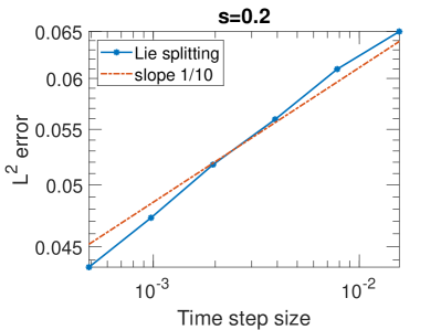
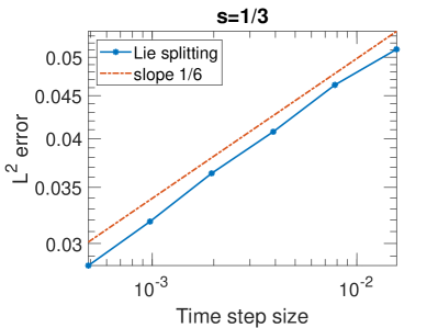
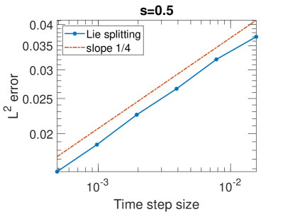
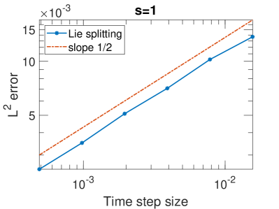
Figure 1. $L^{2}$ error of the Lie splitting scheme for rough initial data $u_{0}\in H^{s}$.   (a) $s=0.2$;  (b) $s={1/3}$;  (c) $s={0.5}$;  (d) $s=1$.

In this section, we numerically illustrate our main result (Theorem 1.1). We display the convergence order of the filtered Lie splitting method with rough initial data. In Figure 1 we consider the periodic NLS (1), discretized with the filtered Lie splitting method (3) and initial data

$$u_{0}=\sum\limits_{k\in\mathbb{Z}^{2}}\langle k\rangle^{-(s+1)}\tilde{g}_{k}e^{i\langle k,x\rangle}\in H^{s},$$

with $s=0.2,~{}1/3,~{}0.5$ and 1, where $\tilde{g}_{k}$ are random variables which are uniformly distributed in the square $[-1,1]+i[-1,1]$. We employ a standard Fourier pseudospectral method for the discretization in space and we choose as largest Fourier mode $K=(2^{12},2^{12})$, i.e., the spatial mesh size $\Delta x=0.0015$ for both of the two space directions. As a reference solution, we use the Lie splitting method with $K$ spatial points and a very small time step size $\tau=2^{-22}$. We choose $T=1$ to be the final time.

From Figure 1, we can clearly find that our numerical experiments confirm the convergence rate of order $\mathcal{O}(\tau^{\frac{s}{2}})$ for solutions in $H^{s}$ (see Theorem 1.1) with $s=0.2,~{}1/3,~{}0.5$ and 1.

We also did some experiments for very small $s$, as for example, $s=0.1$. In this case, the convergence is very slow. To obtain an accurate reference solution for small $s$, one would need an ever increasing number of Fourier modes, which is beyond the capabilities of computers. In Figure 2, we demonstrate that the proven order of convergence only shows up for sufficiently high spatial resolution.

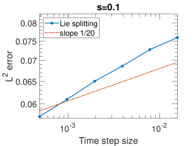
Figure 2. $L^{2}$ error of the Lie splitting scheme for rough initial data $u_{0}\in H^{0.1}$ with different reference solutions. (a) Reference solution with largest Fourier mode $K=(2^{10},2^{10})$, spatial mesh size $\Delta x=0.0061$, and time step size $\tau=2^{-18}$; (b) Reference solution with largest Fourier mode $K=(2^{12},2^{12})$, spatial mesh size $\Delta x=0.0015$, and time step size $\tau=2^{-22}$.

References

- [1] J. Bourgain, Fourier transform restriction phenomena for certain lattice subsets and applications to nonlinear evolution equations. Part I: Schrödinger equations, Geom. Funct. Anal. 3: 209–262 (1993)
- [2] N. Burq, P. Gérard, N. Tzvetkov, Bilinear eigenfunction estimates and the nonlinear Schrödinger equation on surfaces, Inventiones Mathematicae, 159: 187–223 (2005).
- [3] D. De Silva, N. Pavlovic, G. Staffilani and N. Tzirakis, Global well-posedness for a periodic nonlinear Schrödinger equation in 1D and 2D. Discrete Contin. Dyn. Syst. 19, no. 1, 37–65 (2007).
- [4] J. Eilinghoff, R. Schnaubelt, K. Schratz, Fractional error estimates of splitting schemes for the nonlinear Schrödinger equation, J. Math. Anal. Appl. 442:740–760 (2016).
- [5] E. Faou, Geometric Numerical Integration and Schrödinger Equations, European Math. Soc. Publishing House, Zürich 2012.
- [6] L. I. Ignat, A splitting method for the nonlinear Schrödinger equation, J. Differential Equations 250:3022–3046 (2011).
- [7] C. Lubich, On splitting methods for Schrödinger-Poisson and cubic nonlinear Schrödinger equations, Math. Comp. 77:2141–2153 (2008).
- [8] C. Muscalu, W. Schlag, Classical and multilinear harmonic analysis, Cambridge University Press, Cambridge, 2013.
- [9] A. Ostermann, F. Rousset, K. Schratz, Fourier integrator for periodic NLS: low regularity estimates via Bourgain spaces, to appear in J. Eur. Math. Soc.
- [10] A. Ostermann, F. Rousset, K. Schratz, Error estimates at low regularity of splitting schemes for NLS, Math. Comp. 91, 169–182 (2022).
- [11] F. Rousset, K. Schratz, Convergence error estimates at low regularity for time discretizations of KdV, to appear in Pure and Applied Analysis.
- [12] T. Tao, Nonlinear dispersive equations: local and global analysis, Amer. Math. Soc., Providence RI, 2006.
- [13] T. Tao, Poincaré’s legacies, part I: pages from year two of a mathematical blog, Amer. Math. Soc., 2009.