Matching and event-shape NNDL accuracy in parton showers

Abstract

To explore the interplay of NLO matching and next-to-leading logarithmic (NLL) parton showers, we consider the simplest case of $\gamma^{*}$ and Higgs-boson decays to $q\bar{q}$ and $gg$ respectively. Not only should shower NLL accuracy be retained across observables after matching, but for global event-shape observables and the two-jet rate, matching can augment the shower in such a way that it additionally achieves next-to-next-to-double-logarithmic (NNDL) accuracy, a first step on the route towards general NNLL. As a proof-of-concept exploration of this question, we consider direct application of multiplicative matrix-element corrections, as well as simple implementations of MC@NLO and POWHEG-style matching. We find that the first two straightforwardly bring NNDL accuracy, and that this can also be achieved with POWHEG, although particular care is needed in the handover between POWHEG and the shower. Our study involves both analytic and numerical components and we also touch on some phenomenological considerations.

1 Introduction

Next-to-leading order (NLO) accurate event generators have become the de facto tool for the simulation of particle collisions at the LHC. This is in large part due to the success of the two most widely-used NLO matching schemes, MC@NLO Frixione:2002ik and POWHEG Nason:2004rx ; Frixione:2007vw , alongside the two respective computer programs MadGraph5_aMC@NLO Alwall:2014hca and the POWHEG-BOX Alioli:2010xd ; Jezo:2015aia , as well as the independent implementations within the Herwig Bellm:2015jjp ; Reuschle:2016ndi and SHERPA Hoche:2010pf ; Sherpa:2019gpd event generators. These and other matching procedures (e.g. Bauer:2008qh ; Lonnblad:2012ix ; Jadach:2015mza ) were all developed at a time when parton showers had only leading logarithmic accuracy, and one of the questions that was relevant was whether they preserved that leading-logarithmic (LL) accuracy.

In recent years, a number of developments towards next-to-leading logarithmic (NLL) accurate parton showers have taken place Dasgupta:2018nvj ; Dasgupta:2020fwr ; Hamilton:2020rcu ; Karlberg:2021kwr ; Hamilton:2021dyz ; vanBeekveld:2022zhl ; vanBeekveld:2022ukn ; Forshaw:2020wrq ; Holguin:2020joq ; Nagy:2020rmk ; Nagy:2020dvz ; Herren:2022jej , and one can now investigate the interplay between fixed-order matching and higher logarithmic accuracy. To do so, and to help highlight some of the essential considerations that arise, we focus here on the simplest possible process, NLO matching for $\gamma^{*}/Z\to q\bar{q}$ and $H\to gg$ (in the heavy-top limit), using the PanScales family of final-state showers, which all fully satisfy the broad NLL criteria set out in Refs. Dasgupta:2018nvj ; Dasgupta:2020fwr .

Aside from the obvious requirement that matching should preserve the (NLL) logarithmic accuracy of a given shower, the main question that we ask here is whether it can augment the logarithmic accuracy, at least in some situations. To help understand how this might be the case, it is useful to recall the traditional resummation formula for two-jet event shapes and jet rates in two-body decays Catani:1992ua . Specifically, the probability $\Sigma$ for an observable $O$ to have a value below some threshold $e^{L}$ (with $L<0$) is given by

$$\Sigma(O<e^{L})=\left(1+\frac{\alpha_{s}}{2\pi}\,C_{1}+\ldots\right)e^{\alpha_{s}^{-1}g_{1}(\alpha_{s}L)+g_{2}(\alpha_{s}L)+\alpha_{s}g_{3}(\alpha_{s}L)+\dots},\qquad|L|\gg 1\,.$$ (1)

The $g_{1}$ function is responsible for LL terms ($\alpha_{s}^{n}L^{n+1}$), $g_{2}$ for NLL terms ($\alpha_{s}^{n}L^{n}$) and both $C_{1}$ and $g_{3}$ for NNLL terms ($\alpha_{s}^{n}L^{n-1}$). An alternative way of writing $\Sigma$ is

$$\Sigma(O<e^{L})=h_{1}(\alpha_{s}L^{2})+\sqrt{\alpha_{s}}\,h_{2}(\alpha_{s}L^{2})+\alpha_{s}h_{3}(\alpha_{s}L^{2})+\ldots,\qquad|L|\gg 1\,,$$ (2)

where the $h_{1}$ function is responsible for double-logarithmic (DL) terms ($\alpha_{s}^{n}L^{2n}$), $h_{2}$ for NDL terms ($\alpha_{s}^{n}L^{2n-1}$), $h_{3}$ for NNDL terms ($\alpha_{s}^{n}L^{2n-2}$), and so forth. As is well known in the literature on event shapes, NLL resummation automatically implies NDL accuracy, and further inclusion of the $C_{1}$ in Eq. (1) is sufficient to achieve NNDL accuracy Catani:1992ua . In analytical resummation, $C_{1}$ is typically obtained through matching with a NLO calculation. The natural question in a parton shower context is therefore whether matching NLL parton showers with NLO retains the NLL accuracy and additionally achieves NNDL accuracy for two-jet event shapes and the two-jet rate.

In examining this question, we will consider three matching approaches: a straightforward multiplicative matching (similar to the matrix element corrections of Refs. Bengtsson:1986hr ; Seymour:1994df , generalised in Vincia beyond the first order Giele:2007di and related also to the KrkNLO method Jadach:2015mza ), which multiplies the event or splitting weight by the ratio of the true matrix element to the effective shower matrix element for the emission of an extra parton; the MC@NLO method, which adds in the difference between the true matrix element and the effective shower matrix element for the emission of an extra parton; and the POWHEG method, which takes full responsibility for the first emission, and then hands the event over to the shower for the remaining emissions. For the first two, retaining NLL and achieving NNDL accuracy for two-jet event shapes will be relatively straightforward, essentially because the only kinematic region in which they act is the hard region. In contrast, because the POWHEG method always generates the hardest emission, which is often in the infrared (large-logarithm) region, the interplay with the shower logarithmic accuracy is more delicate. Note that understanding the matching/shower interplay of hardest-emission generator (HEG) methods, like POWHEG, is important because such methods also underpin the most widespread NNLO matching approaches, MiNNLO Hamilton:2013fea ; Monni:2019whf and Geneva Alioli:2013hqa (the other main NNLO matching procedure, UNNLOPS Hoche:2014uhw , does not fall into this class).

In Ref. Frixione:2007vw it was shown that the POWHEG Sudakov form factor achieves NLL accuracy for the hardest emission, and in most of this paper we shall take this NLL accuracy of the POWHEG Sudakov as a given. It should be clear that if POWHEG is then followed by a LL shower, that NLL accuracy will be squandered for practical observables. Less straightforward, however, is the question of what happens when POWHEG, with its NLL Sudakov, is followed by a NLL shower.

The subtleties that we have found in the POWHEG case are closely associated with discussions in the literature Catani:2001cc ; Nason:2004rx ; Corke:2010zj about how to connect the effective shower starting scale with the scale of the POWHEG emission. In particular, it is standard to veto the shower branching, so as to provide the correct relation between POWHEG and the shower across the whole of the soft and/or collinear phase space, with no under- or double-counting. With the developments of the past few years on parton shower logarithmic accuracy Dasgupta:2018nvj ; Dasgupta:2020fwr ; Hamilton:2020rcu ; Karlberg:2021kwr ; Hamilton:2021dyz ; vanBeekveld:2022zhl ; vanBeekveld:2022ukn ; Forshaw:2020wrq ; Holguin:2020joq ; Nagy:2020rmk ; Nagy:2020dvz ; Herren:2022jej , it is possible to approach these same questions with a range of new techniques, both analytical and numerical, that help analyse that logarithmic accuracy. In particular, concerns raised at the time of Ref. Corke:2010zj about shower-induced recoil modifying the first (POWHEG) emission are closely connected with the origin of NLL failures discussed in Ref. Dasgupta:2018nvj and, from a NNDL perspective, can be solved once one has NLL shower accuracy: the shower can still modify the first emission, but does so only when the shower emits in the immediate angular and transverse momentum vicinity of the first emission. This ensures that the effect of any modification is NNLL (which also implies that it is beyond NNDL for event shapes). In contrast, the questions of avoiding double- and/or under-counting will relate both with retaining NLL accuracy and the augmentation to NNDL.

In this paper, we will work with an $e^{+}e^{-}$-specific generalisation of POWHEG, which employs an ordering variable that coincides in the soft limit with the generalised PanScales ordering variable, $v\sim k_{t}\theta^{\beta_{\text{{ps}}}}$, parametrised by $\beta_{\text{{ps}}}$. We will refer to it as POWHEG_β. This generalisation enables us to avoid the considerable complications associated with the need for truncated showers Nason:2004rx and the related subtleties of interplay with NLL accuracy. However it leaves open interesting and important questions about the impact of mismatches in the hard-collinear region. As we shall see, these mismatches can arise not only from differences in kinematic maps, but also from the way in which showers partition the $g\to gg$ (and potentially $g\to q\bar{q}$) splitting functions, which effectively breaks their symmetry. Both aspects are relevant for NLL/NNDL accuracy.

Note that the ingredients that we discuss here, while sufficient for event-shape NNDL accuracy, are not enough to obtain NNDL accuracy for more general observables, e.g. for the recently studied sub-jet multiplicities Medves:2022ccw ; Medves:2022uii .

The paper is structured as follows: In section 2 we briefly recall the relevant features of the multiplicative, MC@NLO and POWHEG methods. In section 3 we examine how kinematic mismatches and splitting function de-symmetrisation can affect NNDL accuracy, with both qualitative explanations and explicit calculations. We then verify numerically in section 4 that PanScales showers that are suitably matched to NLO do reach NNDL accuracy for a large set of global event shapes. In section 5 we briefly investigate the impact of the matching schemes in a phenomenological context. We conclude in section 6. Appendix A collects the results for $C_{1}$ coefficients that we use in Eq. (1), Appendix B discusses our treatment of spin correlations in the hard region, including fixed-order validation plots, and Appendix C gives further technical details of our matching procedures.

2 Brief overview of standard matching methods

For an in-depth review of NLO matching procedures, the reader may wish to consult Ref. Nason:2012pr , as well as the original papers. Here we give just a brief overview of the main matching approaches, with notation adapted from Ref. Nason:2021xke so as to be more explicit about the starting scale for the showering following the matched emission. For simplicity, we will ignore the shower cutoff in all of our expressions.

2.1 Multiplicative matching

We start with the simplest kind of matching, multiplicative matching. We write the differential cross section $d\sigma$ in such a way as to make explicit the structure associated with the first (i.e. hardest) emission, schematically

$$\mathrm{d}\sigma_{\text{mult}}=\bar{B}(\Phi_{\rm B})\,\left[S_{\text{\sc ps}}(v_{\Phi}^{\text{\sc ps}},\Phi_{\rm B})\times\frac{R_{\text{\sc ps}}(\Phi)}{B_{0}(\Phi_{\rm B})}\,\mathrm{d}\Phi\otimes\frac{R(\Phi)}{R_{\text{\sc ps}}(\Phi)}\right]\times I_{\text{\sc ps}}(v_{\Phi}^{\text{\sc ps}},\Phi)\,.$$ (3)

Here $\Phi$ is the full Born plus one parton phase space, $\Phi_{\rm B}$ is the underlying Born phase space, and we define the radiation phase space, $\Phi_{\rm rad}$, through $\mathrm{d}\Phi=\mathrm{d}\Phi_{\rm B}\,\mathrm{d}\Phi_{\rm rad}$. In the shower, for a given $\Phi_{\rm B}$ and $\Phi_{\rm rad}$, there is an associated value of a shower ordering variable $v^{\text{\sc ps}}_{\Phi}$. The Born squared matrix element is given by $B_{0}(\Phi_{\rm B})$, the true Born plus one-parton matrix element is $R(\Phi)$. The parton-shower approximation to it, $R_{\text{\sc ps}}(\Phi)$, is expected to coincide with $R(\Phi)$ in the soft and/or collinear limits. The parton-shower Sudakov form factor $S_{\text{\sc ps}}(v,\Phi_{\rm B})$ is given by

$$S_{\text{\sc ps}}(v,\Phi_{\rm B})=\exp\left[-\int_{v_{\Phi}^{\text{\sc ps}}>v}\frac{R_{\text{\sc ps}}(\Phi)}{B_{0}(\Phi_{\rm B})}\mathrm{d}\Phi_{\rm rad}\right],$$ (4)

the NLO normalisation factor can be written

$$\bar{B}(\Phi_{\rm B})=B_{0}(\Phi_{\rm B})+V(\Phi_{\rm B})+\int R(\Phi)\mathrm{d}\Phi_{\rm rad}\,,$$ (5)

where $V(\Phi_{\rm B})$ are the virtual corrections and the factor $I_{\text{\sc ps}}(v_{\Phi}^{\text{\sc ps}},\Phi)$ represents the iterations of the parton shower branching from a value of the shower ordering variable $v_{\Phi}^{\text{\sc ps}}$ onwards. Finally, we use the notation $\otimes$ inside the square brackets to indicate that the first emission is accepted with probability ${R(\Phi)}/{R_{\text{\sc ps}}(\Phi)}$, and if it is not accepted then the attempt to create the first emission continues to lower $v_{\Phi}^{\text{\sc ps}}$. This also effectively replaces $R_{\text{\sc ps}}\to R$ in the integrand of the Sudakov form factor. The main practical difficulty to be aware of in multiplicative matching is the requirement ${R(\Phi)}\leq{R_{\text{\sc ps}}(\Phi)}$, in order for the first emission acceptance probability to be bounded below $1$. From the point of view of logarithmic accuracy, an important feature of Eq. (3) is that when $v_{\Phi}^{\text{\sc ps}}$ is much smaller than the shower starting scale, the matching brings no modifications, because $R_{\text{\sc ps}}=R$ in that region.

2.2 MC@NLO matching

Next we consider the MC@NLO procedure, which can be written as

$$\mathrm{d}\sigma_{\text{MC@NLO}}=\bar{B}_{\text{\sc ps}}(\Phi_{\rm B})\,S_{\text{\sc ps}}(v_{\Phi}^{\text{\sc ps}},\Phi_{\rm B})\times\frac{R_{\text{\sc ps}}(\Phi)}{B_{0}(\Phi_{\rm B})}\,\mathrm{d}\Phi\times I_{\text{\sc ps}}(v_{\Phi}^{\text{\sc ps}},\Phi)\,+\\ +\left[R(\Phi)-R_{\text{\sc ps}}{}(\Phi)\right]\mathrm{d}\Phi\times I_{\text{\sc ps}}(v^{\max},\Phi)\,,$$ (6)

where

$$\bar{B}_{\text{\sc ps}}(\Phi_{\rm B})=B_{0}(\Phi_{\rm B})+V(\Phi_{\rm B})+\int R_{\text{\sc ps}}(\Phi)\mathrm{d}\Phi_{\rm rad}\,.$$ (7)

The interpretation of Eq. (6) is that one generates normal shower events (with a suitable NLO normalisation, $\bar{B}_{\text{\sc ps}}$) and supplements them with a set of hard events, with weights distributed according to $\left[R(\Phi)-R_{\text{\sc ps}}{}(\Phi)\right]$. This last term vanishes in the infrared (and so has a finite integral) because $R_{\text{\sc ps}}$ coincides with $R$ in the soft and/or collinear regions. This is important for logarithmic accuracy, because as for multiplicative matching, it ensures that there is no modification to the showering in the infrared region. Note that there is freedom in MC@NLO as to the choice of shower starting scale in the additional hard events, and here we will use $v^{\max}$, the largest accessible value. Modifying this, e.g. taking $v_{\Phi}^{\text{\sc ps}}$ instead of $v^{\max}$, only affects the $\alpha_{s}^{2}$ contribution in the hard region. Assuming that this multiplies a double-logarithmic Sudakov associated with further emissions, it is expected to affect results at $\alpha_{s}^{n+2}L^{2n}$, which is beyond our target NNDL accuracy.

Our actual implementation of the MC@NLO procedure will differ slightly from Eq. (6) in terms of how we normalise different contributions. The details are given in Appendix C.2, and the differences correspond to NNLO corrections that are anyway beyond the control of NLO matching procedures.

2.3 POWHEG matching

A simple version of the POWHEG method can be written

$$\mathrm{d}\sigma_{\text{POWHEG-simple}}=\bar{B}{}(\Phi_{\rm B})\,S_{\text{\sc heg}}(v_{\Phi}^{\text{\sc heg}},\Phi_{\rm B})\times\frac{R_{\text{\sc heg}}(\Phi)}{B_{0}(\Phi_{\rm B})}\,\mathrm{d}\Phi\times I_{\text{\sc ps}}(v_{\Phi}^{\text{\sc heg}},\Phi)\,,$$ (8)

where the Sudakov form factor $S_{\text{\sc heg}}$ is defined in analogy with Eq. (4) and $R_{\text{\sc heg}}\equiv R$. In this simple version of POWHEG, note the use of $v_{\Phi}^{\text{\sc heg}}$ in $I_{\text{\sc ps}}(v_{\Phi}^{\text{\sc heg}},\Phi)$, i.e. the ordering variable is deduced from the phase space map used with POWHEG (e.g. the FKS Frixione:1995ms map in the POWHEG-BOX), and adopted directly as a shower starting scale for the remaining shower emissions. Throughout this work, when the POWHEG method is used in conjunction with a NLL shower, we will assume that the HEG Sudakov factor $S_{\text{\sc heg}}(v_{\Phi}^{\text{\sc heg}},\Phi_{\rm B})$ is also evaluated with NLL accuracy, i.e. using two-loop running of $\alpha_{s}$ and the CMW scheme Catani:1990rr .

In POWHEG usage with standard transverse-momentum ordered showers, $v_{\Phi}^{\text{\sc heg}}$ in POWHEG and $v_{\Phi}^{\text{\sc ps}}$ in the shower will coincide for a given phase space point when the emission is simultaneously soft and collinear. This is essential in order to achieve leading logarithmic accuracy. This is not, however, naturally the case when using $\beta_{\text{{ps}}}>0$ showers in conjunction with the POWHEG-BOX, because of the latter’s choice of transverse momentum as an ordering variable (which corresponds to $\beta_{\text{{ps}}}=0$). Accordingly, we will adopt a suitably generalised phase space map and ordering variable that satisfies this property also when used with $\beta_{\text{{ps}}}>0$ showers, cf. Appendix C.3. We will call this POWHEG_β. It will be implicit throughout this work that the $\beta$ value in POWHEG_β is always taken equal to $\beta_{\text{{ps}}}$. However, even with POWHEG_β, the two values of $v$ may still differ, for example, when the emission is collinear and hard. This creates a mismatch in the infrared between the phase space covered by the POWHEG_β hardest emission generation and the phase space subsequently covered by the shower. As we shall see in detail in section 3.1, the mismatch has the potential to create NNDL issues, because the logarithmic phase space region associated with the mismatch is of order $1$, the radiation probability in that region comes with one factor of $\alpha_{s}$ and it can then multiply some part of a double logarithmic Sudakov factor, giving an overall $\alpha_{s}^{n+1}L^{2n}$.

The aim of Ref. Corke:2010zj was to eliminate the mismatch. Given the POWHEG first-emission event, the recommended approach within Pythia 8 starts the shower at the maximum allowed scale, but then for each shower emission $i$, based on the kinematics of $i$, the code deduces the equivalent value of the ordering variable in the POWHEG map, $v_{i}^{\text{\sc heg}}$, and discards the emission if $v_{i}^{\text{\sc heg}}>v_{\Phi}^{\text{\sc heg}}$. We write this procedure as

$$\mathrm{d}\sigma_{\text{POWHEG-veto}}=\bar{B}{}(\Phi_{\rm B})\,S_{\text{\sc heg}}(v_{\Phi}^{\text{\sc heg}},\Phi_{\rm B})\times\frac{R_{\text{\sc heg}}(\Phi)}{B_{0}(\Phi_{\rm B})}\,\mathrm{d}\Phi\times I_{\text{\sc ps}}(v^{\max},\Phi|v_{i}^{\text{\sc heg}}<v_{\Phi}^{\text{\sc heg}})\,,$$ (9)

where the additional showering condition is indicated after the vertical bar ($|$) in the $I_{\text{\sc ps}}$ shower iteration factor. This should ensure the absence of holes or double-counting in the infrared phase space (at least when emissions are all well separated). With an important proviso concerning the handling of gluon splitting, discussed below in section 3.2, we expect this to be sufficient to restore NNDL accuracy for event shapes, as long as the underlying shower is NLL accurate.

3 Matching and event-shape NNDL accuracy

In this section we will explore how $\mathcal{O}\left(1\right)$ phase-space mismatches in the collinear and/or soft region affect NNDL accuracy for event shapes, in particular in unvetoed POWHEG style matching, cf. Eq. (8). We will assume that both the shower and the hardest emission generator (HEG) have an ordering variable that coincides, in the soft-collinear region, with the PanScales family of ordering variables,

$$v=\frac{k_{t}}{\rho}e^{-\beta_{\text{{ps}}}|\bar{\eta}|}\,,\qquad\rho=\left(\frac{s_{{\tilde{\imath}}}s_{{\tilde{\jmath}}}}{Q^{2}s_{{\tilde{\imath}}{\tilde{\jmath}}}}\right)^{\frac{\beta_{\text{{ps}}}}{2}}\,,$$ (10)

parametrised by $\beta_{\text{{ps}}}$, and written in terms of the emission transverse momentum $k_{t}$ and $\bar{\eta}$ (which for a back-to-back dipole is essentially a rapidity), as well as $s_{{\tilde{\imath}}{\tilde{\jmath}}}=2{\widetilde{p}}_{i}\cdot{\widetilde{p}}_{j}$, $s_{{\tilde{\imath}}}=2{\widetilde{p}}_{i}\cdot Q$, with $Q$ the total event momentum and the tildes used to represent pre-branching momenta. Recall that $\beta_{\text{{ps}}}=0$ corresponds to transverse-momentum ordering, and that PanGlobal showers are NLL accurate for $0\leq\beta_{\text{{ps}}}<1$, while PanLocal showers are NLL accurate for $0<\beta_{\text{{ps}}}<1$. In Eq. (10), $\rho$ is a quantity that is equal to $1$ for a back-to-back dipole in the event centre-of-mass frame.

As well as parameterising the shower evolution variable in terms of $\beta_{\text{{ps}}}$, it is useful to parameterise event-shape observables in terms of a $\beta_{\text{obs}}$ (cf. Ref. Banfi:2004yd , where it was called $b$). Specifically, when the event has just a single soft-collinear emission, the recursively infrared and collinear safe observable $O$ is given by

$$O_{1\text{-emsn}}=\frac{k_{t}}{Q}e^{-\beta_{\text{obs}}|\eta|}\,,$$ (11)

where $k_{t}$ is again the transverse momentum of the emission and $\eta$ is its rapidity with respect to the emitter. For example, for the thrust Brandt:1964sa ; Farhi:1977sg , $\beta_{\text{obs}}=1$, and for the Cambridge $\sqrt{y_{23}}$ 3-jet resolution scale Dokshitzer:1997in , $\beta_{\text{obs}}=0$. As discussed in the introduction, the quantity we will calculate is the probability $\Sigma(O<e^{L})$ for the observable to be below some threshold (where $L$ is negative).

Our discussion will be in two parts. In section 3.1 we will consider the purely kinematic differences between the HEG and shower maps, which brings a logarithmic analysis to the arguments of Ref. Corke:2010zj . In section 3.2 we will examine additional important considerations that arise for gluon splitting, connected with the widespread procedure in parton showers of partitioning the symmetric $g\to gg$ and $g\to q\bar{q}$ splitting functions into two asymmetric versions, one for each dipole (in the $g\to gg$ case, each containing just a single soft divergence).

3.1 Kinematic mismatch between HEG and shower maps

3.1.1 Qualitative discussion of double-counting

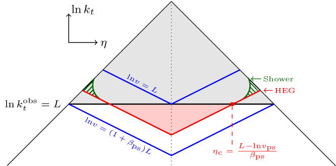
Figure 1: Lund plane Andersson:1988gp representation of the phase space for soft and/or collinear emission, and illustration of the interplay between a hardest emission generator (HEG), a parton shower and a constraint on an observable (black line). Dimensionful quantities ($k_{t}$, $v$) are taken normalised to the centre-of-mass energy $Q$.

The case we shall concentrate on is that where $\beta_{\text{obs}}=0$ and $\beta_{\text{{ps}}}>0$. This is represented in Fig. 1. The threshold on the observable is represented by the horizontal black line. We imagine a shower whose ordering variable coincides with the HEG in the soft limit, but in the hard-collinear region, for a given value of the ordering variable, generates a configuration that is somewhat harder than the HEG (by a factor of order one). This is illustrated with the green shower contour bending upwards relative to the red HEG contour. Though schematic, for simple $e^{+}e^{-}\to q\bar{q}$ events, this picture captures the essence of a $\beta_{\text{{ps}}}=\frac{1}{2}$ extension of POWHEG together with the PanLocal $\beta_{\text{{ps}}}=\frac{1}{2}$ shower.

It is clear that to have $O<e^{L}$, the HEG emission must be below the upper blue contour in Fig. 1, i.e. it must satisfy $\ln v<L$. If the HEG emission occurs between the two blue lines (e.g. on the red line), at a rapidity that places it below the black line (i.e. the observable threshold), the event will contribute to $\Sigma(O<e^{L})$ only if the shower does not emit further above the black line. That probability is given by the initial HEG Sudakov multiplied by the part of the remaining shower Sudakov that is above the black line. The fundamental problem is that the shaded region between the HEG (red) and shower (green) curves will be accounted for twice, once in the HEG Sudakov and once in the shower Sudakov, resulting in an over-suppression of $\Sigma(O<e^{L})$.

More generally we expect the following properties to hold: for contour mismatches in the hard-collinear region we anticipate NNDL artefacts for $\beta_{\text{obs}}<\beta_{\text{{ps}}}$. We do not expect an NNDL artefact for $\beta_{\text{obs}}\geq\beta_{\text{{ps}}}$. In particular, $\beta_{\text{obs}}>\beta_{\text{{ps}}}$ would correspond to a version of Fig. 1 where the black observable-constraint contour is steeper than the two blue shower contours, so the mismatch region is always below the observable-constraint contour and so does not affect the observable. An analogous argument can be made concerning potential contour mismatches in the soft large-angle region, for which we anticipate NNDL artefacts when $\beta_{\text{obs}}>\beta_{\text{{ps}}}$. For the case of $e^{+}e^{-}\to\text{2 jets}$, in the context of the PanScales showers and our specific POWHEG_β formulation, there is no mismatch in this region. However, the issue of soft large-angle mismatches becomes important to address when the Born configuration involves dipoles that are not back-to-back, for example $e^{+}e^{-}\to\text{3 jets}$ or $pp\to Z+\text{jet}$. Such configurations are beyond the scope of this work.

Below, we will give explicit calculations in the context of a double logarithmic approximation. Before doing so it is useful, however, to consider why it is that the HEG/shower combination can achieve NLL accuracy. Let us assume that the HEG and shower contours align in the soft and/or collinear region and also that the shower is NLL accurate (as is the HEG Sudakov). A crucial point to keep in mind is that the only difference between running the HEG and then the shower, or instead just the shower, is an $\mathcal{O}\left(\alpha_{s}\right)$ relative correction to the overall normalisation, as well as the coefficient of the $\mathcal{O}\left(\alpha_{s}\right)$ probability of having an emission in the hard region. Both are NNLL effects. Aside from this, the shower continues after the HEG in exactly the same way as it would had the first emission come from the shower. It is for this reason that the result maintains NLL accuracy.

One comment is that the agreement of contours can be arranged either by a vetoing procedure as in Eq. (9), or by adapting the design of the HEG and/or the shower such that their contours match naturally. This latter approach, while requiring more tailoring of the HEG/shower combination, has the advantage that it eliminates complexities associated with the implementation of the vetoing procedure, complexities that are likely to add extra challenges as one extends showers to higher logarithmic accuracy.

3.1.2 Evaluation of the discrepancy for $\beta_{\text{obs}}=0$, $\beta_{\text{{ps}}}>0$

To make the argument quantitative, we will essentially work in a double-logarithmic (DL) approximation for the event shape distribution, and then specifically evaluate the subleading logarithmic effect of the mismatch. We will need the form of the HEG Sudakov, which we write in pure DL form as

$$S_{\text{\sc heg}}(v)=\exp\left(-\frac{{\bar{\alpha}}\ln^{2}v}{1+\beta_{\text{{ps}}}}\right)\,,\qquad{\bar{\alpha}}\equiv\frac{2C\alpha_{s}}{\pi}\,,$$ (12)

where $C=C_{F}$ for a $q\bar{q}$ event and $C_{A}$ for a $gg$ event, and the HEG uses the same $\beta$ as the parton-shower $\beta_{\text{{ps}}}$. As a first step, it is instructive to consider how we obtain the analogous pure DL form for $\Sigma(O<e^{L})$ in a scenario where there is no mismatch between HEG and shower contours. It is given by

$$\Sigma(O<e^{L}) =e^{-{\bar{\alpha}}(1+\beta_{\text{{ps}}})L^{2}}+e^{-{\bar{\alpha}}L^{2}}\int_{(1+\beta_{\text{{ps}}})L}^{L}d\ell\frac{2{\bar{\alpha}}(L-\ell)}{\beta_{\text{{ps}}}}\exp\left[-{\bar{\alpha}}\frac{(L-\ell)^{2}}{\beta_{\text{{ps}}}}\right],$$ (13a)

$$=e^{-{\bar{\alpha}}L^{2}}\,,$$ (13b)

where the first term in Eq. (13a) is the probability for the HEG emission to be below the lower blue contour in Fig. 1, $\ln v_{\text{\sc heg}}<(1+\beta_{\text{{ps}}})L$, i.e. it corresponds to $S_{\text{\sc heg}}(e^{(1+\beta_{\text{{ps}}})L})$. The second term is the integral for the HEG emission to be between the two blue contours, with two additional conditions. A first condition is that the HEG emission should be on the part of the HEG (red) contour that is below the observable constraint (black line) $\ln k_{t}<L$, which corresponds to a requirement

$$|\eta|<|\eta_{c}|=\frac{L-\ln v_{\text{\sc ps}}}{\beta_{\text{{ps}}}}\,,$$ (14)

where $\ln v_{\text{\sc ps}}\equiv\ell$ in Eq. (13a). The integral over allowed rapidities gives the first factor in the integrand of Eq. (13a). A second condition associated with this integrand is that subsequent shower emissions should also be below the observable constraint (i.e. there should be no emissions in either the grey-shaded triangle, or the pink-shaded triangle). The combination of HEG Sudakov and effective shower Sudakov for this second condition gives the exponential factors in the second (integral) term of Eq. (13a).

As a next step, we consider the impact of the mismatch between the HEG and shower contours, up to NNDL accuracy. The result is almost identical to Eq. (13),

$$\Sigma(O<e^{L}) =e^{-{\bar{\alpha}}(1+\beta_{\text{{ps}}})L^{2}}+e^{-{\bar{\alpha}}L^{2}}\int_{(1+\beta_{\text{{ps}}})L}^{L}\!d\ell\frac{2{\bar{\alpha}}(L-\ell)}{\beta_{\text{{ps}}}}\exp\left[-{\bar{\alpha}}\frac{(L-\ell)^{2}}{\beta_{\text{{ps}}}}-2{\bar{\alpha}}\Delta\right]\!,$$ (15a)

$$=e^{-{\bar{\alpha}}L^{2}}\left[1+2(e^{-{\bar{\alpha}}\beta_{\text{{ps}}}L^{2}}-1){\bar{\alpha}}\Delta+\mathcal{O}\left(\text{N}^{3}\text{DL}\right)\right],$$ (15b)

with just an additional term inside the exponent on the first line, involving a quantity $\Delta$ that represents the effective size of one mismatch region (shaded green in Fig. 1). It arises because of the extra shower phase space that needs to be vetoed when the contours don’t match. For $e^{+}e^{-}\to q\bar{q}$ it reads

$${\bar{\alpha}}\Delta=\int_{0}^{1}d\zeta\frac{\alpha_{s}C_{F}}{2\pi}p_{qq}(\zeta)\cdot 2\ln\frac{\theta^{\text{\sc ps}}_{ik}(v,\zeta)}{\theta^{\text{\sc heg}}_{ik}(v,\zeta)}\,,$$ (16)

where $p_{qq}(\zeta)=(1+\zeta^{2})/(1-\zeta)$ is the reduced $q\to qg$ splitting function and $\theta^{\text{\sc ps}}_{ik}(v,\zeta)$ is the ${\tilde{\imath}}\to ik$ splitting angle in the parton shower for a given value of the ordering variable $v$ and post-splitting quark momentum fraction $\zeta$; $\theta^{\text{\sc heg}}_{ik}(v,\zeta)$ is the analogue for the HEG. For the HEG/shower combinations that we consider, the ratio of angles in Eq. (16) will always be independent of $v$.

A key feature of Eq. (15b) is that the correction is indeed NNDL and starts at order $\alpha_{s}^{2}L^{2}$. Furthermore it vanishes for $\beta_{\text{{ps}}}=0$ (i.e. $\beta_{\text{{ps}}}=\beta_{\text{obs}}$ since we have taken $\beta_{\text{obs}}=0$ in our calculation). This is consistent with our expectation that the discrepancy is present only for $\beta_{\text{obs}}<\beta_{\text{{ps}}}$.

To concretely evaluate Eq. (16), we need to know the $\theta_{ik}(v,\zeta)$ functions in the collinear limit. For the PanLocal and PanGlobal showers Dasgupta:2020fwr and for our extension of POWHEG as given in Appendix C.3, we have

PanLocal: $$\qquad\theta_{ik}(v,\zeta)=2\cdot\left(\frac{v}{Q}\right)^{\frac{1}{1+\beta_{\text{{ps}}}}}(1-\zeta)^{\frac{\beta_{\text{{ps}}}}{1+\beta_{\text{{ps}}}}}\cdot\frac{1}{\zeta(1-\zeta)}\,,$$ (17a)

PanGlobal, POWHEG_β: $$\qquad\theta_{ik}(v,\zeta)=2\cdot\left(\frac{v}{Q}\right)^{\frac{1}{1+\beta_{\text{{ps}}}}}(1-\zeta)^{\frac{\beta_{\text{{ps}}}}{1+\beta_{\text{{ps}}}}}\cdot\frac{1}{1-\zeta}\,.$$ (17b)

Note that the equations are identical except in the last factor, which differs because in PanLocal, the emitter acquires the transverse recoil, while in PanGlobal that transverse recoil is shared across through a boost of the whole event (which in the collinear limit leaves the $ik$ angle unchanged). In the case where we use PanGlobal or POWHEG as HEG followed by the PanLocal shower, combining Eqs. (17) with Eq. (16) results in the following expression for ${\bar{\alpha}}\Delta$:

$${\bar{\alpha}}\Delta =\int_{0}^{1}d\zeta\frac{\alpha_{s}C_{F}}{2\pi}p_{qq}(\zeta)\cdot 2\ln\frac{\theta^{\text{\sc ps}}_{ik}}{\theta^{\text{\sc heg}}_{ik}}\,,$$ (18a)

$$=\int_{0}^{1}d\zeta\frac{\alpha_{s}C_{F}}{2\pi}p_{qq}(\zeta)\cdot 2\ln\frac{1}{\zeta}\,,$$ (18b)

$$=\frac{2C_{F}\alpha_{s}}{\pi}\cdot\frac{4\pi^{2}-15}{24}\,.$$ (18c)

For $H\to gg$, a similar calculation (with values of $w_{gg}=w_{qg}=0$ for the parameters governing the de-symmetrisation of the gluon splitting functions, see section 3.2) gives

$${\bar{\alpha}}\Delta=\frac{\alpha_{s}}{\pi}\frac{C_{A}(12\pi^{2}-49)+8T_{R}n_{f}}{36}\,.$$ (19)

A final comment is that the NNDL-breaking effects discussed here can also be thought of as a violation of the PanScales conditions that there should not be long-range correlations between emissions at disparate rapidities. Specifically, without vetoing, the presence of a soft-collinear HEG emission is effectively changing the probability of a hard-collinear shower emission. As a result, the HEG/shower combination fails to reproduce the factorisation that is present in physical matrix elements for emissions at disparate angles. This also impacts the analytical resummation structure. To see how, we take $\Sigma$ from Eq. (15b), and extract the highest power $L$ at each order in $\alpha_{s}$, which gives

$$\ln\Sigma=-{\bar{\alpha}}L^{2}-\sum_{n=2}^{\infty}\frac{2\beta_{\text{{ps}}}^{n-1}\Delta}{(n-1)!}\cdot{\bar{\alpha}}^{n}L^{2n-2}+\mathcal{O}\left({\bar{\alpha}}^{n}L^{2n-3}\right)\,.$$ (20)

The result clearly fails to satisfy the exponentiation property of Eq. (1), specifically the absence of terms $\alpha_{s}^{n}L^{m}$ in $\ln\Sigma$ with $m>n+1$. This can be viewed as similar, qualitatively, to the spurious super-leading logarithms seen in Ref. Dasgupta:2020fwr (supplemental material, section 3) for standard dipole showers with observables such as the thrust. Below, when we summarise matched shower results together with their logarithmic accuracy, we will use the notation NLL, to remind the reader that the formal NLL accuracy has been lost. One subtlety, however, is that the difference between Eqs. (15b) and (13b) is always of relative order $\alpha_{s}$. This has the consequence that in numerical NLL tests with $\alpha_{s}\to 0$ for fixed $\alpha_{s}L$, this difference would mimic a NNLL term, i.e. NLL accuracy would appear to be preserved despite the presence of spurious super-leading logarithms.

There are, nevertheless, observables that see a larger relative effect. One example is the invariant mass or transverse momentum of the first SoftDrop splitting when using $\beta_{\text{SD}}=0$ Dasgupta:2013ihk ; Larkoski:2014wba . The special characteristic of this observable is that it is not a standard global event shape, and its resummation does not have double-logarithmic terms, i.e. it starts from $g_{2}$ in Eq. (1). In the fixed-coupling approximation that we have effectively used in this section, the SD cross section has the following single-logarithmic structure,

$$\Sigma_{\text{SD}}(L)=e^{{\bar{\alpha}}cL}\,,$$ (21)

where $c$ is a constant that depends on SoftDrop’s $z_{\text{cut}}$ parameter, which we take to be small. Using the same strategy as above, one can explore how Eq. (21) is modified in HEG/shower combinations with a hard-collinear mismatch. Keeping $\beta_{\text{{ps}}}=0$ for simplicity, one finds

$$\Sigma_{\text{SD}}(L)=e^{{\bar{\alpha}}cL-{\bar{\alpha}}\Delta}+e^{-{\bar{\alpha}}L^{2}}(1-e^{-{\bar{\alpha}}\Delta})\,,$$ (22)

where the coefficient $\Delta$ that parameterises the impact of the HEG/shower contour mismatch now depends on $z_{\text{cut}}$. As with Eq. (20), this generates spurious $\alpha_{s}^{n}L^{2n-2}$ terms. If we examine the derivative of $\Sigma_{\text{SD}}$ (as we will do below in our phenomenology plots),

$$\partial_{L}\Sigma_{\text{SD}}(L)={\bar{\alpha}}c\,e^{{\bar{\alpha}}cL-{\bar{\alpha}}\Delta}-2{\bar{\alpha}}Le^{-{\bar{\alpha}}L^{2}}(1-e^{-{\bar{\alpha}}\Delta})\,,$$ (23)

we observe that there is a region, $L\sim 1/\sqrt{\alpha_{s}}$, where the second term is suppressed relative to the first only by $\sqrt{\alpha_{s}}$. Thus in this region, the impact of the HEG/shower mismatch is parametrically larger than the relative $\mathcal{O}\left(\alpha_{s}\right)$ correction seen in Eq. (15b).

3.2 Additional subtleties for gluon splitting

The purpose of this section is to discuss an issue that can arise even when we have a HEG/shower combination whose kinematic contours (for a fixed value of the evolution variable) are aligned not just in the soft-collinear region, but for any single-emission phase-space point that is soft and/or collinear. The issue is connected with the fact that the $g\to gg$ splitting function

$$\frac{1}{2!}P_{gg}(\zeta)=C_{A}\left(\frac{\zeta}{1-\zeta}+\frac{1-\zeta}{\zeta}+\zeta(1-\zeta)\right)\,,$$ (24)

has two soft divergences, one for $\zeta\to 0$ and the other for $\zeta\to 1$. This is a consequence of the inherent symmetry $\zeta\leftrightarrow(1-\zeta)$, which stems from the fact that $g\to gg$ corresponds to splitting to two identical particles (hence also the $1/2!$ factor). However, dipole showers break this symmetry, through the concept of an emitting particle (the “emitter”) and a radiated particle. In particular, in order to help reproduce the correct pattern of large-angle soft radiation, dipole showers de-symmetrise the splitting function so that there is a divergence only when the radiated gluon becomes soft. For example the PanScales showers use

$$\frac{1}{2!}P_{gg}^{\text{asym}}(\zeta)=C_{A}\left[\frac{1+\zeta^{3}}{1-\zeta}+(2\zeta-1)w_{gg}\right]\,,$$ (25)

where the choice of the $w_{gg}$ parameter fixes arbitrariness that arises in partitioning the finite part of the splitting function. It is straightforward to verify that $P_{gg}^{\text{asym}}(\zeta)+P_{gg}^{\text{asym}}(1-\zeta)=2P_{gg}(\zeta)$.

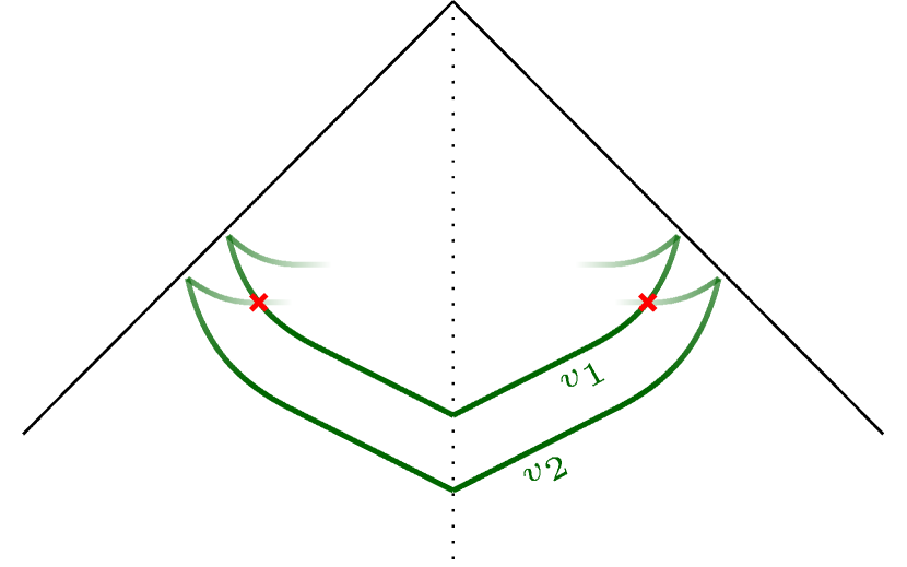
(a)

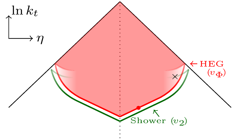
(b)

Figure 2: Schematic illustration of the issue associated with gluon asymmetrisation. (a) Contours on the Lund plane, in the PanLocal family of showers, highlighting the fact that a given physical point $X$ in the Lund plane (highlighted with a red cross) can come from two different values of $v$. The shading of the green curves represents the variation in radiation intensity along the contour. (b) Density plot, at each point in the Lund plane, representing schematically the fraction of the emission intensity at that point that has been excluded once the HEG has reached a given $v$ value ($v_{\Phi}$) without emitting, and an illustration that as the shower continues there may still be phase-space points (such as that marked with a cross) where the Sudakov has only been partially accounted for. The implications are discussed in the text.

The hard matrix element generated by the HEG can be de-symmetrised similarly. The POWHEG-BOX code follows the FKS procedure Frixione:1995ms , which introduces so-called $\mathcal{S}$-functions that are used to partition the soft and collinear singularities. The de-symmetrisation discussed above is handled by an additional multiplicative factor $h(\zeta)$, cf. Eqs. (2.76)–(2.77) of Ref. Frixione:2007vw , with $\zeta$ for an ${\tilde{\imath}}\to ik$ splitting defined as $E_{i}/(E_{i}+E_{k})$. One can implement the scheme of Eq. (25) by setting

$$h(\zeta)=\frac{P_{gg}^{\text{asym}}(\zeta)}{P_{gg}(\zeta)}.$$ (26)

The reason that the de-symmetrisation matters is that in many cases the kinematic map is not symmetric under $\zeta\leftrightarrow(1-\zeta)$. This can be seen in Eqs. (17), where the only combination that is symmetric is the PanLocal map for $\beta_{\text{{ps}}}=0$ (this, however, is not NLL accurate). The asymmetry is illustrated for PanLocal $\beta_{\text{{ps}}}=\frac{1}{2}$ in Fig. 2a, which shows fixed-$v$ contours in the physical Lund plane. Specifically for emission of $k$ from an ${\tilde{\imath}}{\tilde{\jmath}}$ Born event, i.e. ${\tilde{\imath}}{\tilde{\jmath}}\to ijk$, the plot represents $\ln k_{t}=\ln[\min(E_{i},E_{k})\sin\theta_{ik}]$ versus $\eta=-\ln\tan\theta_{ik}/2$ in the right-hand Lund plane, and analogously in the left-hand plane with respect to $j$. A given contour has two parts: the lower branch corresponds to $\zeta>\frac{1}{2}$, and contains the soft divergence; the upper branch corresponds to $\zeta<\frac{1}{2}$ and is free of any soft divergence, so it contributes significantly only in the hard collinear region.

The critical observation is that any specific point $X$ in the hard-collinear region of the Lund plane can be populated by two distinct values of $v$: first at some $v_{1}$ by the lower ($\zeta>\frac{1}{2}$) part of the $v_{1}$ contour, and then at a smaller value of $v=v_{2}<v_{1}$ by the upper ($\zeta<\frac{1}{2}$) part of the $v_{2}$ contour. The relative fraction of radiation intensity from the two values of $v$ at a given point in the Lund plane depends on how the splitting function has been de-symmetrised, for example on the value of $w_{gg}$ in Eq. (25). For a given shower or HEG, we will refer to $f_{X,1}(w_{gg})$ as the fraction coming from the $v_{1}$ contour and $f_{X,2}(w_{gg})=1-f_{X,1}(w_{gg})$ as the fraction from the $v_{2}$ contour.

Fig. 2b illustrates how this is relevant in the combination of HEG and shower. Suppose that we have a HEG with some $w_{gg}=w^{\text{\sc heg}}$ and a shower with some $w_{gg}=w^{\text{\sc ps}}$. We consider a situation where the HEG generated the first emission at some $v_{\Phi}$, and where that emission is deep into the soft-collinear region, so that the branching should have no direct kinematic impact on subsequent hard collinear radiation. Next, let us focus on the point labelled with a cross (“$X$”). That point is associated with two values of the evolution variable, $v_{1}$ and $v_{2}$ (remember, the map from evolution variable to kinematic contour is identical between HEG and shower across the full soft and/or collinear phase space). The first value, $v_{1}$ is already excluded by virtue of the fact that the HEG’s emission corresponded to a smaller value of $v$, i.e. $v_{\Phi}<v_{1}$. In effect some fraction $f_{X,1}(w_{\text{\sc heg}})$ of the total Sudakov for not emitting at $X$ was the HEG’s responsibility, and that fraction depends on the de-symmetrisation parameter $w^{\text{\sc heg}}$ of the HEG. The second value of the evolution variable, $v_{2}$, that is associated with kinematic point $X$ is the shower’s responsibility, since $v_{2}<v_{\Phi}$. If the shower does not emit there, the fraction of the total Sudakov that the shower contributes is $f_{X,2}(w^{\text{\sc ps}})\equiv 1-f_{X,1}(w^{\text{\sc ps}})$. If $w^{\text{\sc heg}}=w^{\text{\sc ps}}$ then those two fractions add up to one. Otherwise they may be larger or smaller than one, which is equivalent to having a partial double- or under-counting of the radiation intensity at $X$, or more generically in the hard-collinear vicinity of the $v_{\Phi}$ contour.

The impact of the double counting will be similar to that of the kinematic-contour mismatch discussed in section 3.1. Indeed all that needs doing to evaluate its NNDL effect is to take Eq. (15b) and replace the expression for ${\bar{\alpha}}\Delta$ in Eq. (16) with

$${\bar{\alpha}}\Delta=\int_{0}^{\frac{1}{2}}d\zeta\left[\frac{1}{2!}P_{gg}^{\text{\sc ps}}(\zeta)-\frac{1}{2!}P_{gg}^{\text{\sc heg}}(\zeta)\right]\cdot 2\ln\frac{\theta_{ik}(v,\zeta)}{\theta_{ik}(v,1-\zeta)}\,,$$ (27)

where $\theta_{ik}(v,\zeta)$ is the same function for both the HEG and the parton shower. To understand Eq. (27), keep in mind that $0<\zeta<\frac{1}{2}$ is the region corresponding to the upper part of the contour in Fig. 2. If $P_{gg}^{\text{\sc ps}}(\zeta)>P_{gg}^{\text{\sc heg}}(\zeta)$ then the combination of HEG and shower is enhancing the Sudakov in that region, much like the double counting of Fig. 1. The impact of the double counting on the event shape is structurally similar to that of the mismatch of contours in section 3.1. It can in fact be thought of as a weighted mismatch of contour, moving the mismatched part of the weight from $\theta_{ik}(v,1-\zeta)$ to $\theta_{ik}(v,\zeta)$, from which one deduces Eq. (27).

Note that there is a similar consideration for $g\to q\bar{q}$ branchings, where the splitting function is sometimes also de-symmetrised. For completeness, using the PanScales form for the de-symmetrised $g\to q\bar{q}$ splitting,

$$P_{qg}^{\text{asym}}(\zeta)=T_{R}n_{f}\left[2\zeta^{2}-(2\zeta-1)w_{qg}\right]\,,$$ (28)

we have

$${\bar{\alpha}}\Delta^{\text{PanGlobal}} =\left[\left(w^{\text{\sc heg}}_{gg}-w^{\text{\sc ps}}_{gg}\right)C_{A}-\left(w^{\text{\sc heg}}_{qg}-w^{\text{\sc ps}}_{qg}\right)n_{f}T_{R}\right]\frac{-1}{1+\beta_{\text{{ps}}}}\,,$$ (29a)

$${\bar{\alpha}}\Delta^{\text{PanLocal}} =\left[\left(w^{\text{\sc heg}}_{gg}-w^{\text{\sc ps}}_{gg}\right)C_{A}-\left(w^{\text{\sc heg}}_{qg}-w^{\text{\sc ps}}_{qg}\right)n_{f}T_{R}\right]\frac{\beta_{\text{{ps}}}}{1+\beta_{\text{{ps}}}}\,,$$ (29b)

Note that we will usually choose $w^{\text{\sc heg}}_{gg}=w^{\text{\sc heg}}_{qg}\equiv w^{\text{\sc heg}}$ and $w^{\text{\sc ps}}_{gg}=w^{\text{\sc ps}}_{qg}\equiv w^{\text{\sc ps}}$, which leads to an almost complete cancellation between the $C_{A}$ and $n_{f}T_{R}$ terms for $n_{f}=5$ (the cancellation would be exact for $n_{f}=6$). Accordingly, when we come to test the above analysis numerically with the full shower below, we will use $n_{f}=0$ so as to avoid this cancellation.

As with the kinematic mismatch of section 3.1, the effect that we have just seen corresponds to a violation of the PanScales conditions that there should not be long-range correlations between emissions at disparate rapidities, i.e. the presence of a soft-collinear emission (from the HEG) modifies the probability for subsequent hard-collinear emission (from the shower). This, again, has implications for exponentiation.

3.3 Practical implementation of vetoing

For completeness, we give here the specific algorithm that we adopt to achieve the vetoing of parton shower emissions following on from a first HEG step. The combination in which we will use it is with a POWHEG or PanGlobal-like HEG, followed by a PanLocal shower (dipole or antenna). This combination has the property (cf. Eq. (17)) that we only have to deal with double-counting, never with holes in soft and/or collinear phase space. The algorithm comes in two parts.

One part keeps track of the indices of the particles that should be considered the descendants of the particles in the Born configuration $\Phi_{\rm B}$. For our cases later of $e^{+}e^{-}\to q\bar{q}$ and $H\to gg$, we label the Born partons $a$ and $b$. For any branching (HEG or shower) where the emitter is one of the partons currently labelled as Born, e.g. ${\tilde{\imath}}\to ik$ with ${\tilde{\imath}}$ a Born particle, the more energetic of $i$ and $k$ inherits the Born label. Note that for a $q\to qg$ splitting we could alternatively have considered the descendent quark to always be the Born particle. We will discuss the relevance of the choice below.

The second part of the algorithm follows the various HEG and shower steps:

1. Allow the HEG to generate the first emission, resulting in a Born$+1$ configuration $\Phi$, with a value $v_{\Phi}^{\text{\sc heg}}$ of the HEG ordering variable. The HEG step updates the Born indices as per above.

2. Start the parton shower with $v^{\text{\sc ps}}=v_{\Phi}^{\text{\sc heg}}$. This is allowed because our HEG/shower combinations can lead to double counting, but not holes in the soft and/or collinear phase space.

3. For all subsequent emissions $k$ from a dipole ${\tilde{\imath}}{\tilde{\jmath}}$, if the emitter ${\tilde{\imath}}$ carries a Born label, check the following veto condition:

   1. Compute $k_{t}=E_{k}\sin\theta_{ik}$ and $\eta=-\ln\tan\theta_{ik}/2$ (this is done using exact momenta).

   2. Compare these coordinates with the corresponding contour of the HEG at $\ln v_{\Phi}^{\text{\sc heg}}$, i.e. $\ln k_{t}^{\text{\sc heg}}(v_{\Phi}^{\text{\sc heg}},\eta)=\ln v_{\Phi}^{\text{\sc heg}}+\beta_{\text{{ps}}}|\eta|$ for POWHEG_β and for PanGlobal as a HEG.

   3. If the emission is above the contour, $\ln k_{t}>\ln k_{t}^{\text{\sc heg}}(v_{\Phi}^{\text{\sc heg}},\eta)$, veto the emission.

   For antenna showers, where the emitter/spectator distinction is absent, the same check is performed for either end of the dipole, insofar as it has the Born label.

4. If the splitting is accepted, update the Born labels.

A few comments may be helpful. The first concerns the freedom in how we assign the Born label. For NNDL accuracy, the critical element is that when Born-labelled parton ${\tilde{\imath}}$ splits as ${\tilde{\imath}}\to ik$, then when $k$ is a soft gluon, it should be $i$ that acquires the Born label. When $k$ is a hard gluon, subsequent vetoing only affects triple-collinear configurations (and their associated virtual corrections), i.e. configurations with three partons at commensurate angles and with commensurate energies. Those do not play a role at NNDL accuracy. A second comment concerns the shower starting scale, which we could equally well have taken to be $v^{\text{\sc ps}}=v^{\max}$, as written in Eq. (9), as long as emissions from non-Born partons are only allowed for $v^{\text{\sc ps}}<v_{\Phi}^{\text{\sc heg}}$. This should not affect NNDL accuracy, and we have verified that in a phenomenological context the impact is small, at the percent level. Were we to consider HEG/shower combinations that result in IR holes, there would be less freedom in the choice of shower starting scale and it might well be necessary to start with $v^{\text{\sc ps}}=v^{\max}$. Finally, it is useful to be aware that the kinematic variables that we adopt for the contour check in step 3b differ from the Lund contours represented in Fig. 2, specifically with the use of $E_{k}$ rather than $\min(E_{i},E_{k})$. Insofar as the meaning of $\zeta>\frac{1}{2}$ is the same in the HEG and the shower, this helps avoid complications with the folding of contours seen with the $\min(E_{i},E_{k})$ choice in Fig. 2. However it is still necessary, in the $g\to gg/q\bar{q}$ case, to ensure that the same de-symmetrisation of the splitting functions is used in the HEG and shower steps.

4 Logarithmic tests

	mult.	MC@NLO	POWHEGβ	HEG${}_{\text{PanGlobal}}$
PanLocal $\beta_{\text{{ps}}}=0.5$ (dip.)	✓	✓	✓${}_{\!\!(v)}$
PanLocal $\beta_{\text{{ps}}}=0.5$ (ant.)		✓		✓${}_{\!\!(v)}$
PanGlobal $\beta_{\text{{ps}}}=0.0$	✓	✓	✓
PanGlobal $\beta_{\text{{ps}}}=0.5$	✓	✓	✓

Table 1: The main matching and shower combinations for which we will test NNDL accuracy, for both $\gamma^{*}/Z\to q\bar{q}$ and $H\to gg$. A $(v)$ next to a check mark indicates that we use the vetoing algorithm of section 3.3. We use the NODS colour scheme from Ref. Hamilton:2020rcu .

We now turn to logarithmic tests with event shapes. There are quite a few potential combinations of matching scheme and shower. The subset that we explore is listed in Table 1. The combinations that do not have a check mark would also have been straightforward to test, and are left out simply to limit CPU usage and bookkeeping.

We have run the standard NLL tests as in Refs. Dasgupta:2020fwr ; Hamilton:2020rcu at $<1\%$ target accuracy, to verify that the matched showers continue to reproduce full-colour NLL accuracy for global event shapes (and NDL for multiplicity at $\lesssim 2\%$ target accuracy). These tests were successful. Given the large number of results, we refrain from showing them. Instead, here we concentrate on the NNDL accuracy tests.

For the NNDL predictions we take the standard NLL formulae as used in earlier work and supplement them with the $C_{1}$ coefficients as given in Appendix A, some taken from the literature, some extracted numerically for this work. Slightly adapting the notation of the introduction, we denote by $\Sigma(\alpha_{s},L)$ the probability for an event shape observable to have a value $O$ that is less than $e^{L}$ for a given $\alpha_{s}(Q)=\alpha_{s}$ where $Q$ is the $\gamma^{*}\to q\bar{q}$ centre-of-mass energy, or the Higgs-boson mass for $H\to gg$ tests. For a matched shower to qualify as being accurate at the NNDL level, its prediction for the cumulative distribution of a given observable, $\Sigma_{\text{PS}}$, must clearly satisfy the following criterion,

$$\lim_{\begin{subarray}{c}\alpha_{s}\to 0\\ \xi\,\text{fixed}\end{subarray}}\frac{\Sigma_{\text{\sc ps}}(\alpha_{s},-\sqrt{\xi/\alpha_{s}})-\Sigma_{\rm NNDL}(\alpha_{s},-\sqrt{\xi/\alpha_{s}})}{\alpha_{s}\Sigma_{\rm DL}}=0\,,$$ (30)

where fixing $\xi$ is equivalent to fixing $\alpha_{s}L^{2}$, as is relevant for isolating different terms in the DL-type expansion of Eq. (2).

To perform the tests, we run the showers with up to six values of $\alpha_{s}=\frac{0.1}{N^{2}}$, with $N\in\{3,4,5,6,8,12\}$. We will show results at $\xi=\alpha_{s}L^{2}=1.296$ for $\gamma^{*}\to q\bar{q}$, and $\xi=\alpha_{s}L^{2}=0.791$ for $H\to gg$, which correspond to values of the cumulative distributions $0.25\leq\Sigma\leq 0.6$, i.e. in the bulk of the distribution for all observables under scrutiny. In each run, we choose a shower cutoff such that showering continues substantially below the smallest value needed to accurately predict the observable at the given $\xi$ value. The limit in Eq. (30) is extracted numerically by extrapolating a fit that is linear or quadratic in powers of $\sqrt{\alpha_{s}}$. In $\gamma^{*}\to q\bar{q}$ events, we use a linear polynomial fit to the three smallest $\alpha_{s}$ values. We repeat the fit with the four smallest $\alpha_{s}$ values and take the difference in the intercept of both fits as a systematic uncertainty for the extrapolation procedure. In $H\to gg$ events, we find that there is still a visible quadratic component for some observables at the $\alpha_{s}$ and $\xi$ values we are considering, and thus fit a quadratic polynomial to all $\alpha_{s}$ values (all but the largest for the systematic uncertainty).

We will consider a range of observables with different values of $\beta_{\text{obs}}$, cf. Eq. (11). Given the discussion of section 3, which showed that the presence of potential NNDL artefacts depends in a non-trivial way on the choice of both $\beta_{\text{obs}}$ and $\beta_{\text{{ps}}}$, it is important to ensure that for each type of matching, we have shower/event-shape combinations with $\beta_{\text{obs}}<\beta_{\text{{ps}}}$, $\beta_{\text{obs}}=\beta_{\text{{ps}}}$ and $\beta_{\text{obs}}>\beta_{\text{{ps}}}$. The observables that we take are

• The Cambridge $\sqrt{y_{23}}$ resolution parameter Dokshitzer:1997in , total and wide jet broadenings $B_{T}$ and $B_{W}$ Catani:1992ua , which all have $\beta_{\text{obs}}=0$ (i.e. the same LL and NDL structures), but differ at NLL and NNDL.

• The thrust Brandt:1964sa ; Farhi:1977sg , and the $C$-parameter Ellis:1980wv ; Parisi:1978eg ; Donoghue:1979vi . These both have $\beta_{\text{obs}}=1$, and are equivalent up to NLL (considering $C/6$ versus $1-T$), but not at NNDL.

• Three sets of parameterised observables for $\beta_{\text{obs}}=0,\frac{1}{2},1$: the fractional moments ${\rm FC}_{1-\beta_{\text{obs}}}$ of the energy-energy correlations Banfi:2004yd , as well as the sum and maximum, $\sum_{i}k_{T,i}/Qe^{-\beta_{\text{obs}}|\eta_{i}|}$ and $\max_{i}k_{T,i}/Qe^{-\beta_{\text{obs}}|\eta_{i}|}$ respectively, among primary Lund declusterings $i$ Dreyer:2018nbf ; Dasgupta:2018nvj . The first two observables are equivalent to each other at NLL accuracy but differ at NNDL, while the latter differs also in its NLL terms.

Figure 3: Results of the NNDL accuracy tests at fixed $\xi=\alpha_{s}L^{2}$ for the PanLocal dipole and antenna (with $\beta_{\text{{ps}}}=\frac{1}{2}$) and PanGlobal ($\beta_{\text{{ps}}}=0$ and $\beta_{\text{{ps}}}=\frac{1}{2}$) showers, without 3-jet matching, for $\gamma^{*}\to q\bar{q}$ (top) and $H\to gg$ (bottom). In these and subsequent plots, points marked green (red) show agreement (disagreement) with the NNDL results at the $2\sigma$-level. Amber points manifest coincidental agreement for $n_{f}=5$ as explained in the text. The plots of this figure have no green points.

We start by showing results for Eq. (30) for showers without matching, in order to gauge the size of the NNDL discrepancy. This is shown in Fig. 3. Points are coloured in green if the central value is consistent with zero within $2\sigma$ (and in red otherwise), where the $1\sigma$-uncertainty band is given by the statistical uncertainty and a systematic fit uncertainty added linearly. With the exception of the PanGlobal shower in $H\to gg$, all showers without matching are clearly inconsistent with the NNDL result and the discrepancy can be significant, notably for the PanLocal showers where it is of order $2{-}$3. The PanGlobal $H\to gg$ results are marked in amber, because the agreement is fortuitous: while the shower’s effective 3-jet matrix-element is different from the exact result, we found that a coincidental cancellation leads to a seemingly correct result at $n_{f}=5$. For each shower, the discrepancy is independent of the observable, because the test is carried out for small values of the observable (since $\alpha_{s}L^{2}$ is fixed with $\alpha_{s}\to 0$), while the mismatch between the effective shower matrix element and the true matrix element is limited to the hard region.

Figure 4: Results of NNDL accuracy tests for the PanLocal dipole ($\beta_{\text{{ps}}}=\frac{1}{2}$) and PanGlobal ($\beta_{\text{{ps}}}=0,\frac{1}{2}$) showers, matched with the multiplicative scheme.

Next, we examine results of the matching with the multiplicative scheme. Fig. 4 displays the results of NNDL tests for the PanLocal dipole ($\beta_{\text{{ps}}}=\frac{1}{2}$) and the PanGlobal ($\beta_{\text{{ps}}}=0,\frac{1}{2}$) showers matched multiplicatively. These are all in agreement with the NNDL result for all observables.

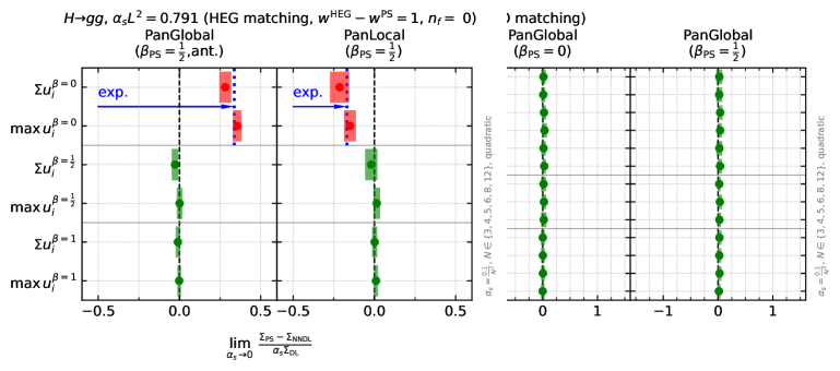
Figure 5: Results of the NNDL accuracy tests for the PanScales showers (see Fig. 3) matched with the MC@NLO scheme.

In Fig. 5, we show results of the NNDL tests where the PanScales showers are matched with the MC@NLO scheme. Here as well, the matched showers correctly reproduce all observables resummed to NNDL accuracy.

Figure 6: Results of NNDL accuracy tests for the four HEG/shower combinations shown in Table 1.

We now turn to the case of POWHEG matching. As summarised in Table 1, we use either POWHEG_β as a HEG, or PanGlobal ($\beta_{\text{{ps}}}=\frac{1}{2}$). In Fig. 6, four HEG/shower combinations are shown: PanGlobal + PanLocal antenna ($\beta_{\text{{ps}}}=\frac{1}{2}$), POWHEG_β + PanLocal dipole ($\beta_{\text{{ps}}}=\frac{1}{2}$) and POWHEG_β + PanGlobal ($\beta_{\text{{ps}}}=0,\frac{1}{2}$). Where the PanLocal (dipole or antenna) shower is used as the main shower, we veto emissions according to the algorithm presented in section 3.3. For all combinations presented in Fig. 6, we also align the choice of de-symmetrisation in the gluon splitting functions, $w^{\text{\sc heg}}=w^{\text{\sc ps}}=0$, following the analysis of section 3.2. Results are all in agreement with NNDL.

Figure 7: Results of NNDL accuracy tests for two combinations of HEG and shower whose contours do not match in the hard-collinear region, all with $\beta_{\text{{ps}}}=\frac{1}{2}$. The showers are matched with the POWHEG scheme, but the vetoing procedure given in section 3.3 is not applied, in order to highlight the NNDL discrepancy expected for observables with $\beta_{\text{obs}}<\beta_{\text{{ps}}}$. The expected value from Eqs. (18)–(19) is shown in dotted blue (and marked by the blue arrow labelled “exp.”).

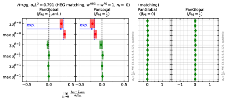
Figure 8: Results of NNDL accuracy tests with $n_{f}=0$ for the PanGlobal and PanLocal showers ($\beta_{\text{{ps}}}=\frac{1}{2}$), using the same shower as both a HEG and for the subsequent parton showering steps, but with different choices of the de-symmetrisation parameter in the gluon splitting function, $w^{\text{\sc heg}}=1$, and $w^{\text{\sc ps}}=0$ respectively. The expected value of the NNDL discrepancy for $\beta_{\text{obs}}=0$ from Eqs. (29a)–(29b) is shown in dotted blue.

Finally, we showcase the NNDL discrepancy arising from a failure to take the considerations of section 3 into account when matching showers with the POWHEG scheme. In Fig. 7, we display results of the NNDL tests for two combinations of HEG/shower which require vetoing due to kinematic mismatch (PanGlobal + PanLocal antenna $\beta_{\text{{ps}}}=\frac{1}{2}$, and POWHEG_β + PanLocal $\beta_{\text{{ps}}}=\frac{1}{2}$, see Table 1), but where we deliberately do not apply the veto algorithm of section 3.3. As anticipated, disabling the veto has a visible effect for observables with $\beta_{\text{obs}}<\beta_{\text{{ps}}}$. The expected discrepancy for $\beta_{\text{obs}}=0$, which can be obtained by inserting Eq. (18c) (for $\gamma^{*}\to q\bar{q}$) or Eq. (19) (for $H\to gg$) into Eq. (15b), is plotted as a blue dotted line. That value is in agreement with the observed discrepancy from the showers.

Similarly, we can investigate whether the numerical results confirm the expected NNDL discrepancy stemming from the misaligned de-symmetrisation of the gluon splitting functions presented in section 3.2. We show results of NNDL tests for a configuration where one of the PanGlobal or PanLocal showers (with $\beta_{\text{{ps}}}=\frac{1}{2}$), is used as a HEG, followed by the same shower for subsequent emissions. In order to see the discrepancy of section 3.2, we choose different values of the de-symmetrisation parameter $w_{gg}$, see Eq. (25), for the first emission ($w^{\text{\sc heg}}$) and for the rest of the showering ($w^{\text{\sc ps}}$). As can be seen from Eqs. (29a) and (29b), the discrepancy in both cases is proportional to $C_{A}-n_{f}T_{R}$. In order to avoid the large cancellation of this effect with $n_{f}=5$, in Fig. 8 we run with $n_{f}=0$, and we set $w^{\text{\sc heg}}=1$ and $w^{\text{\sc ps}}=0$. While we could have extracted the $C_{1}$ coefficients numerically for $n_{f}=0$ as well, in Fig. 8 we only show observables for which the analytic form of $C_{1}$ is available. Recall that we only expect a discrepancy for $\beta_{\text{obs}}<\beta_{\text{{ps}}}$. Though the NNDL discrepancy associated with mismatched $w^{\text{\sc heg}}\neq w^{\text{\sc ps}}$ is numerically smaller than for the case of the kinematic mismatch (note the different scale on the $x$-axis of Fig. 8), we find that the results agree with our analytic predictions for them, both when there are discrepancies and when there are none.

5 Phenomenological considerations

In this last section, we briefly explore the interplay of matching and logarithmic accuracy with physical choices for the coupling and values of observables, as opposed to the asymptotic values used in the preceding sections. The intent at this stage is not to be exhaustive, nor to compare to data (for that we would still like to have finite quark mass effects and an interface to hadronisation), but rather to get some insight into how logarithmic-accuracy improvements affect practical distributions.

We will show parton-level results with a preliminary estimate of uncertainties, specifically taking an envelope of two sources of uncertainty: (1) renormalisation scale variation and (2) uncertainties associated with residual lack of control of shower matrix elements beyond the matched emission.

The scale uncertainties are calculated according to Ref. vanBeekveld:2022ukn ’s adaptation of the prescription by Mrenna and Skands Mrenna:2016sih . Specifically, for showers that are NLL accurate, we take the emission intensity to be proportional to

$$\alpha_{s}(\mu_{\text{{r}}}^{2})\left(1+\frac{K\alpha_{s}(\mu_{\text{{r}}}^{2})}{2\pi}+2\alpha_{s}(\mu_{\text{{r}}}^{2})b_{0}(1-z)\ln x_{\text{{r}}}\right)\,,\qquad\mu_{\text{{r}}}=x_{\text{{r}}}\mu_{\text{{r}}}^{\text{central}}\,.$$ (31)

Here $z$ is the fraction of the emitter momentum carried away by the radiation, while $b_{0}$ and $K$ are the usual $\beta$-function and CMW Catani:1990rr coefficients, and $\mu_{\text{{r}}}^{\text{central}}$ is the emission transverse momentum ($\kappa_{\perp}$) as defined in the shower. The factor of $1-z$ ensures that NLO scale compensation is present for soft-collinear emissions, but turned off for hard emissions. Scale variation will be probed by taking $x_{\text{{r}}}=\{\frac{1}{2},1,2\}$. We will use this scale variation also in the matching, e.g. so that HEG-style matching has the correct scale compensation in the infrared. Throughout, we use the NODS colour scheme Hamilton:2020rcu (i.e. full-colour NLL for global event shapes), a two-loop coupling, with $\alpha_{s}(m_{Z}^{2})=0.118$, $5$ light flavours and an infrared cutoff implemented such that $\alpha_{s}(\mu_{\text{{r}}}^{2})$ is set to zero for $\mu_{\text{{r}}}<x_{\text{{r}}}\times 0.5\;\mathrm{GeV}$.

We will also show results with our PanScales implementation Dasgupta:2020fwr of the Pythia 8  shower Sjostrand:2004ef (which we call PSPythia 8). Since it is a LL shower, we will not include the scale compensating terms in Eq. (31) for shower emissions (nor for the HEG emission), however we do include a two-loop running and the CMW constant term $K$.

To estimate the uncertainty associated with lack of control of shower matrix-elements in the hard region, we modify the default shower splitting probability according to

$$P_{\text{splitting}}(x_{\text{hard}})=P_{\text{splitting}}^{\text{(default)}}\times\left[1+(x_{\text{hard}}-1)\min\left(\frac{4\kappa_{\perp}^{2}}{Q^{2}},1\right)\right]\,,$$ (32)

where $x_{\text{hard}}=1$ reproduces the default splitting probability and we take as variations $x_{\text{hard}}=\{\frac{1}{2},1,2\}$. As with the scale variation, there is some arbitrariness in these choices and their detailed implementation, whose full investigation we leave to future work together with that of other potential sources of uncertainty. For unmatched shower results, we apply Eq. (32) to all splittings, while for matched shower results we apply it to all but the first emission. The results are shown without spin correlations, but we have verified for the multiplicative matching procedure that they have a numerically negligible impact on the event-shape type observables shown here (and no impact up to NLL/NNDL). Note that fixed-order tests of spin correlations with matching are given in Appendix B.

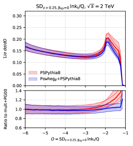
Figure 9: Thrust (left), Cambridge $\ln y_{23}$ (middle) and SoftDrop $\ln k_{t}/Q$ (right) distributions, unmatched (red) and matched (blue). They are obtained with a LL shower (our PanScales implementation of the Pythia 8 shower (PSPythia 8, top row)) and two NLL showers: PanGlobal with $\beta_{\text{{ps}}}=0$ (middle row) and PanLocal $\beta_{\text{{ps}}}=\frac{1}{2}$ (bottom row). The last row also shows the impact of HEG-style matching without the veto discussed in section 3.3. Dotted lines show $x_{\text{hard}}$ variation, while dashed lines show $x_{\text{{r}}}$ variations.

Fig. 9 shows parton-level results for the thrust and Cambridge $\ln y_{23}$ at $\sqrt{s}=m_{Z}$. It also features a SoftDrop (SD) $\ln k_{t}/Q$ distribution, with $z_{\text{cut}}=0.25$, $\beta_{\text{SD}}=0.0$ Dasgupta:2013ihk ; Larkoski:2014wba and $k_{t}$ for a ${\tilde{\imath}}\to ik$ splitting defined as $\min(E_{i},E_{k})\sin\theta_{ik}$. The choice of $z_{\text{cut}}=0.25$ is larger than commonly used, and helps concentrate on the hard-collinear region. The SoftDrop procedure is applied to each of the two jets as obtained from a $2$-jet Cambridge clustering. This observable is shown for $\sqrt{s}=2\;\mathrm{TeV}$ insofar as it is intended to be illustrative of an LHC jet substructure observable.

The top row of Fig. 9 shows results for our implementation of the Pythia 8 shower. Recall that since this shower is LL rather than NLL we do not include the scale compensation terms of Eq. (31) when varying the renormalisation scale (neither in the shower itself, nor in the POWHEG_β stage). The remaining rows show the PanGlobal shower with $\beta_{\text{{ps}}}=0$ and the PanLocal (dipole) shower $\beta_{\text{{ps}}}=\frac{1}{2}$. Without matching, there are large uncertainties in the $3$-jet region, mostly dominated by the $x_{\text{hard}}$ variations (dotted lines). Once matching is turned on, it is the scale uncertainties that dominate the uncertainty bands over the full range shown for the event shapes. Note that the scale compensation that is used in the NLL shower brings a visible reduction in uncertainty as compared to the case of LL showers.

Observe also that POWHEG_β matching with the PanLocal shower without the kinematic veto, shown in the lower row (green band), induces a noticeable shift in the kinematic distributions. Curiously, this is true not just for the $\ln y_{23}$ distribution (where there is a NNDL effect), but also for the thrust (where there is no NNDL effect, but still a kinematic double-counting). The clearest effect is seen for the SoftDrop observable at intermediate values of $\ln k_{t}/Q$. This is not unexpected: recall from the discussion at the end of section 3.1 that for moderately large values of the logarithm, $L\sim 1/\sqrt{\alpha_{s}}$, the impact of the HEG/shower contour mismatch is expected to be of relative order $\sqrt{\alpha_{s}}$ rather than at most $\alpha_{s}$ for standard global event shapes.

In Fig. 9 it was possible to show only a limited number of matching/shower combinations. To help visualise characteristics of a wider range shower/matching combinations, we select a specific bin in each of two distributions, $0.14<1-T<0.15$, and the SoftDrop $-3.1<\ln k_{t}/Q<3.0$, chosen so as to be in a transition region between the large-logarithm and hard $3$-jet regimes. We then examine the ratio of a range of showers and matching schemes to the multiplicatively-matched PanGlobal $\beta_{\text{{ps}}}=0$ result. This is shown in Figs. 10 and 11, with one row for each shower/matching combination.

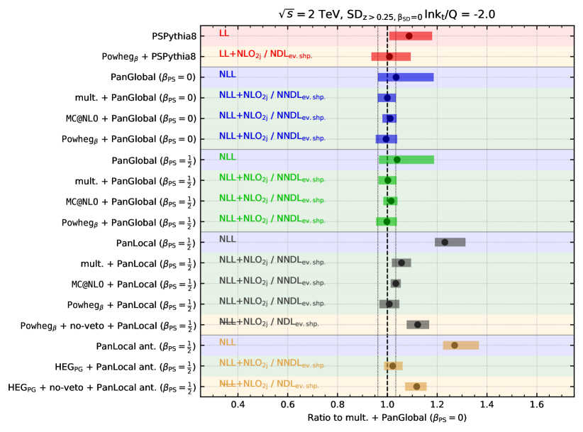
Figure 10: Ratio of multiple shower/matching scheme combinations to the multiplicatively-matched PanGlobal $\beta_{\text{{ps}}}=0$ shower in a bin $0.14<1-T<0.15$ of the thrust distribution. The error bands represent the scale uncertainty and are colour-coded differently for each “main” shower, while the background colour reflects the accuracy of the matching/shower combination, i.e. LL (red), LL+NLO_2j/NDL_ev.shp. or NLL+NLO_2j/NDL_ev.shp. (yellow), NLL (blue), and NLL+NLO_2j/NNDL_ev.shp. (green). The thin dotted vertical lines indicate the size of the scale uncertainties for the reference results, i.e. multiplicatively-matched PanGlobal $\beta_{\text{{ps}}}=0$. Recall from section 3.1 that the NLL notation indicates a breaking of exponentiation.

Figure 11: Analogue of Fig. 10 for the $k_{t}/Q$ distribution of the splitting from the SoftDrop ($z_{\text{cut}}=0.25,\beta_{\text{SD}}=0$) procedure, in a bin $-3.1<\ln k_{t}/Q<-3.0$.

Features to note beyond those observed for Fig. 9 are: (1) The matched NLL showers have uncertainties that are broadly similar across matching and shower combinations (somewhat larger for PanLocal $\beta_{\text{{ps}}}=\frac{1}{2}$), and consistent with each other to within uncertainties. Note that the residual $10\%$ variation between matched showers could have a significant impact on tuning, and ideally one should include $3$-jet NLO matching, e.g. as done in Ref. Hartgring:2013jma . (2) The characteristics seen in Fig. 9 for POWHEG_β matching with PanLocal (dipole) $\beta_{\text{{ps}}}=\frac{1}{2}$ without the kinematic veto appear to be replicated also when using the PanGlobal shower as a HEG (HEG${}_{\text{PG}}$) in combination with the PanLocal (antenna) shower without a veto, suggesting that they are genuinely an impact of the lack of veto rather than a coincidence.

Overall the results in this section highlight the importance of both matching and NLL accuracy and of bringing them together consistently, lending support to the practical value of pursuing the programme to improve shower logarithmic accuracy.

6 Conclusions

The simple framework of two-body decays that we have studied here provides a clean and powerful laboratory to explore the interplay of parton-shower logarithmic accuracy and matching. In particular, we have seen that NLO matching can augment the accuracy of NLL showers, so that they additionally attain NNDL accuracy for global event shapes. This was relatively straightforward to achieve with multiplicative and MC@NLO matching methods, because they alter the shower behaviour or add events only in the hard region. In contrast, with matching methods such as POWHEG that take responsibility for generating the hardest emission, an extra element is needed, which is to ensure that the hardest-emission generator and shower align in their generation of phase space in the full soft and/or collinear regions. Failing to account for this prevents the HEG/shower combination from attaining NNDL accuracy. Furthermore, it subtly compromises NLL accuracy, generating spurious super-leading logarithms, Eq. (20), that resum in such a way, Eq. (15b), as to vanish in standard numerical NLL accuracy global event-shape tests (but not necessarily for single logarithmic observables, such as SoftDrop with $\beta_{\text{SD}}=0$). In this paper we used the (standard) approach of vetoing shower steps in order to avoid double-counting phase space already generated with the HEG. However, thinking forward to possible approaches to achieving yet higher logarithmic accuracy, it is likely to be advantageous to consider designing HEG tools such that they have the freedom to mimic the lowest order soft/collinear phase-space generation of any given shower.

A related and more subtle issue occurs when a given phase-space point can be reached from more than one value of the HEG or shower ordering variable. In our study, this issue arose in the context of de-symmetrisation of gluon splitting functions in the hard-collinear region, cf. section 3.2. However, we expect it to be relevant more generally also in processes with non-trivial soft large-angle structures, for example in the presence of three or more Born partonic legs. The critical observation is that in such situations, the HEG and the shower must have the same relative weights for each of the distinct values of the ordering variable that can lead to that phase-space point.

The numerical tests of section 4 provided extensive validation of our understanding of parton-shower NNDL event-shape accuracy. The results confirmed NNDL accuracy in the situations where we expected to achieve it, and furthermore reproduced the analytic expectations for discrepancies in situations with kinematic or de-symmetrisation mismatches.

In section 5, we took first steps towards the exploration of the phenomenological impact of logarithmically accurate showers, including preliminary uncertainty estimates. Perhaps the main conclusion to be drawn so far is that there is good consistency across different matching schemes and showers, to within the uncertainties, as well as significant reductions in uncertainties relative to LL showers. Furthermore, matching/shower combinations that do not achieve NNDL accuracy appear to give predictions in tension with those from NNDL-accurate showers. Clearly next important phenomenological steps include interfacing with hadronisation, the inclusion of heavy quark masses, comparisons to data and associated exploration of tuning NLL showers.

Appendix A $C_{1}$ coefficients

In this Appendix, we report the numerical values for the $C_{1}$ coefficients that enter into the NNDL resummation. These can be found in Table 2, alongside analytical expressions where these can be found in literature. The numerical values are quoted for $C_{A}=3$, $C_{F}=\frac{4}{3}$ and $n_{f}=5$ and the statistical error on the last digit is reported in the brackets.

The numerical extraction of $C_{1}$ is performed with our own matrix-element integrator. It uses the phase space of Ref. Dokshitzer:1992ip for the $\gamma\rightarrow q\bar{q}$ channel and the phase space of Ref. Cox:2018wce for the $H\rightarrow gg$ channel which is better suited due to the symmetric nature of the $H\rightarrow ggg$ process. The relevant matrix elements are given by

$$\frac{|\mathcal{M}_{\gamma\rightarrow q(1)\bar{q}(2)g(3)}|^{2}}{\sigma_{0}} =\frac{\alpha_{s}C_{F}}{2\pi}\frac{x_{1}^{2}+x_{2}^{2}}{(1-x_{1})(1-x_{2})},$$ (33)

$$\frac{|\mathcal{M}_{h\rightarrow g(1)g(2)g(3)}|^{2}}{\sigma_{0}} =\frac{\alpha_{s}C_{A}}{6\pi}\frac{1+(1-x_{1})^{4}+(1-x_{2})^{4}+(1-x_{3})^{4}}{(1-x_{1})(1-x_{2})(1-x_{3})},$$ (34)

$$\frac{|\mathcal{M}_{h\rightarrow g(1)q(2)\bar{q}(3)}|^{2}}{\sigma_{0}} =\frac{\alpha_{s}n_{f}T_{R}}{\pi}\frac{(1-x_{2})^{2}+(1-x_{3})^{2}}{1-x_{1}},$$ (35)

where $x_{i}$ is the energy fraction of the $i$-th particle, and $\sigma_{0}$ refers to the underlying Born cross section for the processes $\gamma\rightarrow q\bar{q}$ and $H\rightarrow gg$ respectively. In the limit where any of the global event shapes that we study in this paper go singular the cumulative distribution takes the form of Eq. (1), and at fixed first order can be written in the form Catani:1991kz

$$\Sigma(O<e^{L})=1+\frac{\alpha_{s}}{2\pi}\,[\,G_{12}\,L^{2}+G_{11}\,L+C_{1}\,]\,,$$ (36)

where the constants $G_{mn}$ depend only on the infrared and collinear scaling of the global event shape, and can be extracted from CAESAR Banfi:2004yd . In order to extract $C_{1}$ it is therefore enough to compute numerically the normalised cumulative distribution in the singular region, subtracting the two logarithmic terms analytically. In practice we go to values of $\ln\mathcal{O}\sim-16$ and have excellent agreement with the known coefficients, where available.

x Observable $\gamma^{*}\to q\bar{q}$ $H\to gg$ Numerical Analytic Numerical Analytic $\sqrt{y_{23}}$ -6.685(2) $C_{F}\left(-6\ln 2+\frac{\pi^{2}}{6}-\frac{5}{2}\right)$ Banfi:2001bz -13.417(6) $B_{T}$ 1.825(2) $C_{F}\left(\pi^{2}-\frac{17}{2}\right)$ Becher:2012qc 6.438(5) $B_{W}$ 1.825(2) $C_{F}\left(\pi^{2}-\frac{17}{2}\right)$ Becher:2012qc 6.438(5) $\Sigma\,u_{i}^{\beta=0.0}$ -4.492(2) $C_{F}\left(-6\ln 2+\frac{\pi^{2}}{3}-\frac{5}{2}\right)$ Medves:2022ccw -8.482(5) $C_{A}\left(-\frac{22}{3}\ln 2+\frac{\pi^{2}}{3}-\frac{44}{9}\right)+n_{f}\left(\frac{4}{3}\ln 2+\frac{25}{18}\right)$ Medves:2022ccw $\mathrm{max}\,u_{i}^{\beta=0.0}$ -4.492(2) $C_{F}\left(-6\ln 2+\frac{\pi^{2}}{3}-\frac{5}{2}\right)$ Medves:2022ccw -8.482(5) $C_{A}\left(-\frac{22}{3}\ln 2+\frac{\pi^{2}}{3}-\frac{44}{9}\right)+n_{f}\left(\frac{4}{3}\ln 2+\frac{25}{18}\right)$ Medves:2022ccw ${\rm FC}_{1}$ 1.825(2) 6.439(5) $\Sigma\,u_{i}^{\beta=0.5}$ -2.9013(16) $C_{F}\left(-4\ln 2+\frac{\pi^{2}}{9}-\frac{1}{2}\right)$ Medves:2022ccw -6.595(4) $C_{A}\left(-\frac{44}{9}\ln 2+\frac{\pi^{2}}{9}-\frac{127}{54}\right)+n_{f}\left(\frac{8}{9}\ln 2+\frac{23}{27}\right)$ Medves:2022ccw $\mathrm{max}\,u_{i}^{\beta=0.5}$ -2.9013(16) $C_{F}\left(-4\ln 2+\frac{\pi^{2}}{9}-\frac{1}{2}\right)$ Medves:2022ccw -6.595(4) $C_{A}\left(-\frac{44}{9}\ln 2+\frac{\pi^{2}}{9}-\frac{127}{54}\right)+n_{f}\left(\frac{8}{9}\ln 2+\frac{23}{27}\right)$ Medves:2022ccw ${\rm FC}_{\frac{1}{2}}$ 1.3106(16) 3.352(3) $\Sigma\,u_{i}^{\beta=1.0}$ -2.1066(13) $C_{F}\left(-3\ln 2+\frac{1}{2}\right)$ Medves:2022ccw -5.650(3) $C_{A}\left(-\frac{11}{3}\ln 2-\frac{13}{12}\right)+n_{f}\left(\frac{2}{3}\ln 2+\frac{7}{12}\right)$ Medves:2022ccw $\mathrm{max}\,u_{i}^{\beta=1.0}$ -2.1066(13) $C_{F}\left(-3\ln 2+\frac{1}{2}\right)$ Medves:2022ccw -5.650(3) $C_{A}\left(-\frac{11}{3}\ln 2-\frac{13}{12}\right)+n_{f}\left(\frac{2}{3}\ln 2+\frac{7}{12}\right)$ Medves:2022ccw $1-T$ 1.0522(13) $C_{F}\left(\frac{\pi^{2}}{3}-\frac{5}{2}\right)$ Catani:1992ua 1.810(3) $C$ 5.4381(12) $C_{F}\left(\frac{2\pi^{2}}{3}-\frac{5}{2}\right)$ Catani:1998sf 11.680(3)

Table 2: $C_{1}$ coefficients for the observables under scrutiny in the NNDL tests of section 4. The numerical values are extracted with $C_{A}=3$, $C_{F}=\frac{4}{3}$ and $n_{f}=5$. The observables are organised into three groups with $\beta_{\text{obs}}$ values respectively of $0$, $\frac{1}{2}$ and $1$.

Appendix B Spin correlations in the matching region

The inclusion of spin correlation effects Richardson:2001df ; Fischer:2017htu ; Richardson:2018pvo constitutes a defining component of a NLL-accurate parton shower. Purely collinear Karlberg:2021kwr and soft Hamilton:2021dyz spin correlations were previously included in the PanScales showers, and it was shown that the expected logarithmic structure is reproduced. In this appendix, we briefly validate the extension of the algorithm to account for matching. To the best of our knowledge, analytical and semi-numerical resummation results for spin-sensitive observables such as the triple energy-correlation Chen:2020adz and Lund-declustering azimuthal correlations Karlberg:2021kwr have yet to be extended to include $3$-jet matching. We thus validate the algorithm at fixed-order, where focusing on the matching region is straightforward.

The extension of the Collins-Knowles spin algorithm to account for matched branchings is straightforward (and has been explored already in Ref. Richardson:2018pvo ). As formulated in Ref. Hamilton:2021dyz , the algorithm relies on a two-body hard scattering amplitude $\mathcal{M}_{\text{hard}}^{\lambda_{1}\lambda_{2}}$ that is positioned at the root of the binary tree structure that is used to efficiently transmit spin information. Normally, when a shower branching occurs, a corresponding node is attached to this binary tree that encodes the spin information of the branching. However, when the first branching is matched, one should instead re-initialise the binary tree with the corresponding three-body hard scattering amplitude $\mathcal{M}_{\text{hard}}^{\lambda_{1}\lambda_{2}\lambda_{3}}$. Afterwards, the spin algorithm continues as normal. We implement hard scattering amplitudes for the processes considered in this work, i.e. $e^{+}e^{-}\to\gamma^{*}\to q\bar{q}g$, $H\to ggg$ and $H\to gq\bar{q}$.

The amplitudes are computed following the notation and conventions set out in Ref. Karlberg:2021kwr , where a spinor product is denoted as

$$S_{\lambda}(p,q)=\bar{u}_{\lambda}(p)u_{-\lambda}(q).$$ (37)

$e^{+}e^{-}\to q\bar{q}g$

We denote the amplitude as $M(\lambda_{e^{+}},\lambda_{e^{-}};\lambda_{q},\lambda_{\bar{q}},\lambda_{g})$, where the dependence on the momenta is implicit. The non-vanishing helicity configurations are

$$M(\lambda,-\lambda;\lambda,-\lambda,\lambda) =\frac{S_{-\lambda}(p_{e^{-}},p_{\bar{q}})^{2}\,S_{\lambda}(p_{e^{-}},p_{e^{+}})}{S_{-\lambda}(p_{q},p_{g})\,S_{-\lambda}(p_{\bar{q}},p_{g})},$$ (38)

$$M(\lambda,-\lambda;\lambda,-\lambda,-\lambda) =\frac{S_{\lambda}(p_{e^{+}},p_{q})^{2}\,S_{-\lambda}(p_{e^{-}},p_{e^{+}})}{S_{\lambda}(p_{q},p_{g})\,S_{\lambda}(p_{\bar{q}},p_{g})},$$ (39)

$$M(\lambda,-\lambda;-\lambda,\lambda,\lambda) =-\frac{S_{-\lambda}(p_{e^{-}},p_{q})^{2}\,S_{\lambda}(p_{e^{-}},p_{e^{+}})}{S_{-\lambda}(p_{q},p_{g})\,S_{-\lambda}(p_{\bar{q}},p_{g})},$$ (40)

$$M(\lambda,-\lambda;-\lambda,\lambda,-\lambda) =-\frac{S_{\lambda}(p_{e^{+}},p_{\bar{q}})^{2}\,S_{-\lambda}(p_{e^{-}},p_{e^{+}})}{S_{\lambda}(p_{q},p_{g})\,S_{\lambda}(p_{\bar{q}},p_{g})}.$$ (41)

$H\to ggg$

We denote the amplitude as $M(\lambda_{g_{1}},\lambda_{g_{2}},\lambda_{g_{3}})$. The non-vanishing helicity configurations are

$$M(\lambda,\lambda,\lambda) =-\frac{1}{4}\frac{m_{H}^{4}}{S_{-\lambda}(p_{g_{1}},p_{g_{2}})S_{-\lambda}(p_{g_{2}},p_{g_{3}})S_{-\lambda}(p_{g_{1}},p_{g_{3}})},$$ (42)

$$M(\lambda,\lambda,-\lambda) =-\frac{S_{\lambda}(p_{g_{1}},p_{g_{2}})^{3}}{S_{\lambda}(p_{g_{2}},p_{g_{3}})S_{\lambda}(p_{g_{3}},p_{g_{1}})},$$ (43)

$$M(\lambda,-\lambda,\lambda) =-\frac{S_{\lambda}(p_{g_{3}},p_{g_{1}})^{3}}{S_{\lambda}(p_{g_{1}},p_{g_{2}})S_{\lambda}(p_{g_{2}},p_{g_{3}})},$$ (44)

$$M(-\lambda,\lambda,\lambda) =-\frac{S_{\lambda}(p_{g_{2}},p_{g_{3}})^{3}}{S_{\lambda}(p_{g_{1}},p_{g_{2}})S_{\lambda}(p_{g_{3}},p_{g_{1}})}.$$ (45)

$H\to gq\bar{q}$

We denote the amplitude as $M(\lambda_{g},\lambda_{q},\lambda_{\bar{q}})$. The non-vanishing helicity configurations are

$$M(\lambda,\lambda,-\lambda) =-\frac{S_{\lambda}(p_{q},p_{g})^{2}}{S_{\lambda}(p_{q},p_{\bar{q}})},$$ (46)

$$M(\lambda,-\lambda,\lambda) =\frac{S_{\lambda}(p_{\bar{q}},p_{g})^{2}}{S_{\lambda}(p_{q},p_{\bar{q}})}.$$ (47)

Note that this corresponds to the $H\to gq\bar{q}$ amplitude as mediated by the heavy-top limit of the effective loop-induced $Hgg$ operator, as opposed to gluon emission following a direct $Hqq$ Yukawa interaction.

B.1 Validation

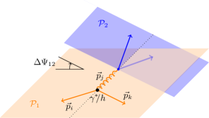
Figure 12: An illustration of the spin-sensitive observable $\Delta\Psi_{12}$ as the difference of the azimuthal angles of the branching plane of the matched emission $\mathcal{P}_{1}$ and the branching plane of a subsequent collinear branching $\mathcal{P}_{2}$.

We validate the implementation of the three-body hard scattering amplitudes at second order by comparing to exact matrix elements of MG5_aMC@NLO Alwall:2014hca . We consider configurations where the first matched emission with momentum $p_{k}$ occurs from a dipole with momenta $\tilde{p}_{i}$ and $\tilde{p}_{j}$ at a relatively large, fixed transverse momentum

$$k_{t,1}/Q=\frac{\sqrt{p_{i}{\cdot}p_{k}\,p_{j}{\cdot}p_{k}}}{Q^{2}}=0.3,$$ (48)

where $p_{i}$ and $p_{j}$ are the post-branching dipole constituents, while varying its rapidity

$$\eta_{1}=\frac{1}{2}\ln\frac{p_{j}{\cdot}p_{k}}{p_{i}{\cdot}p_{k}}.$$ (49)

A second collinear branching then occurs with a small, fixed opening angle $\theta_{2}=10^{-5}$ and collinear momentum fraction $z_{2}=0.4$. When the $3$-jet event is produced via radiation of a gluon, it is the collinear splitting of the radiated gluon that we examine; in $H\to gg$ events where the $3$-jet event is obtained through a $g\to q\bar{q}$ splitting, it is the collinear splitting of the remaining Born gluon that we examine. The difference between the azimuthal orientations of the branching planes $\Delta\Psi_{12}$ is then sensitive to spin correlations. An illustration of this observable is shown in Fig. 12. In particular, the cross section has the form

$$\frac{d\sigma}{d\Delta\Psi_{12}d\eta_{1}}\propto a_{0}(\eta_{1})+a_{2}(\eta_{1})\cos\left(2\Delta\Psi_{12}\right).$$ (50)

The values of $a_{0}$ and $a_{2}$ can be extracted through a Fourier transform. The results are shown in Fig. 13 for $e^{+}e^{-}\to\gamma^{*}\to q\bar{q}$ and in Fig. 14 for $H\to gg$. The ratio $(a_{2}/a_{0})$ is shown for the PanGlobal shower with matching enabled. Furthermore, the ratio between the parton shower $(a_{2}/a_{0})$ and the exact matrix element $(a_{2}/a_{0})$ is shown, confirming that the matched shower reproduces the exact matrix element.

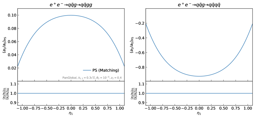
Figure 13: Second-order validation of the implementation of spin correlations in the hard region for $e^{+}e^{-}\to\gamma^{*}\to q\bar{q}$. Following Eq. (50), the ratio $a_{2}/a_{0}$ is computed for the shower with matching enabled (blue curve). Below, the ratio of the shower $a_{2}/a_{0}$ to the exact matrix element $a_{2}/a_{0}$ is shown.

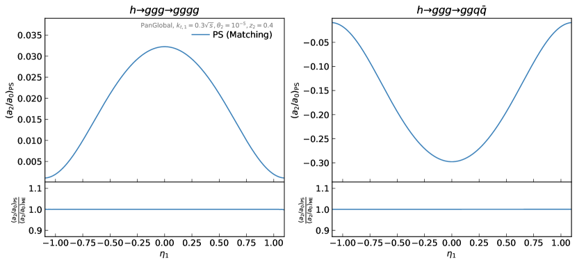
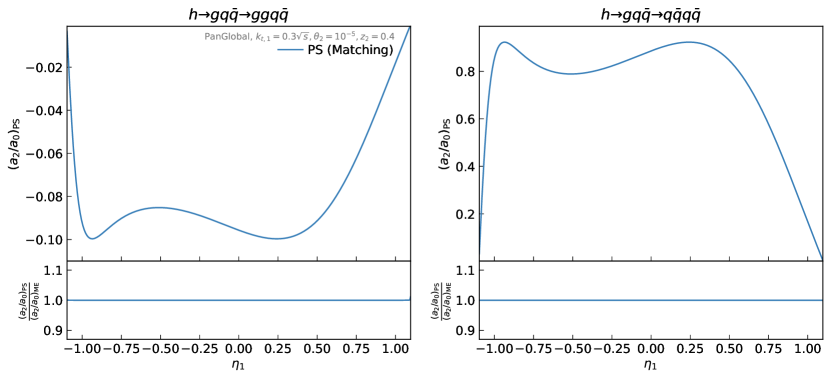
Figure 14: Same as Figure 13, but for all possible configurations of $H\to gg$. Note that in the lower plots, it is the gluon of the underlying 3-jet system that undergoes collinear splitting, rather than the hard emission from the 2-jet system (which is a quark or anti-quark, and so does not mediate azimuthal correlation). This is also the reason for the lack of symmetry in the matched result between positive and negative $\eta_{1}$ values.

Appendix C Technical details of the matching implementation

The tests performed in section 4 require us to probe very small values of $\alpha_{s}$ and very large values of the relevant logarithm. In the parton shower, this corresponds to very small values of the cutoff scale, which in turn requires precise control over the numerical accuracy of the parton shower. If we were to make use of the public implementations of POWHEG Alioli:2010xd and MC@NLO Alwall:2014hca , we would lack this precision. The results of section 4 are thus obtained with a simple dedicated implementation of POWHEG and MC@NLO for the processes at hand within the PanScales framework.

In the following, we provide some details concerning the implementation of multiplicative matching in the PanScales showers, and of the implementation of POWHEG and MC@NLO in the PanScales framework.

C.1 Multiplicative matching

The multiplicative matching of the PanScales showers is accomplished by replacing the usual splitting functions, which are only correct in the soft and collinear limits, by $R(\Phi)/B_{0}(\Phi_{\rm B})$ for the first emission only. In situations where the shower partitions the total emission weight into multiple dipoles or antennae, the same partitioning is applied to the weight $R(\Phi)/B_{0}(\Phi_{\rm B})$. Furthermore, a Jacobian factor must be included to account for the transformation from the radiative phase space to the shower variables.

For completeness, we give here the analytic expressions of the effective one-emission matrix elements for the PanLocal dipole and PanGlobal showers, as well as the Jacobian factor mentioned above. We also briefly discuss a workaround for the issue of under-sampling in the PanGlobal shower, which appears in hard configurations.

C.1.1 PanLocal (dipole)

For the PanLocal dipole shower, the total radiation intensity is a sum over two dipole ends,

$$\frac{R_{\text{\sc ps}}^{\text{\sc pl}}(\Phi)}{B_{0}(\Phi_{\rm B})}\mathrm{d}\Phi_{R} ={\rm d}\mathcal{P}_{\tilde{i}\tilde{j}}^{[\tilde{i}]}+{\rm d}\mathcal{P}_{\tilde{i}\tilde{j}}^{[\tilde{j}]}$$

$$={\rm d\,ln}v\,{\rm d}\bar{\eta}\frac{\alpha_{s}}{\pi}\left[g(\bar{\eta})a_{k}P_{{\tilde{\imath}}\to ik}(a_{k})+({\tilde{\imath}}\leftrightarrow{\tilde{\jmath}})\right]$$

$$={\rm d}x_{i}{\rm d}x_{j}\frac{\alpha_{s}}{\pi}\left[\left|J^{\text{\sc PL}}\right|^{-1}g(\bar{\eta})a_{k}P_{{\tilde{\imath}}\to ik}(a_{k})+({\tilde{\imath}}\leftrightarrow{\tilde{\jmath}})\right]\,,$$ (51)

where the dipole is partitioned at the bisector of the dipole’s opening angle (in the event frame) by a function $g(\bar{\eta})$ (where $\bar{\eta}=\frac{1}{2}\ln\frac{a_{k}}{b_{k}}$),

$$\bar{\eta}\leq-1:g(\bar{\eta})\equiv 0,\quad-1<\bar{\eta}<1:g(\bar{\eta})=\frac{15}{16}\left(\frac{\bar{\eta}^{5}}{5}-\frac{2\bar{\eta}^{3}}{3}+\bar{\eta}+\frac{8}{15}\right),\,\quad\bar{\eta}\geq 1:g(\bar{\eta})\equiv 1\,.$$ (52)

The Dalitz variables $(x_{i},x_{j})$ are related to $(a_{k},b_{k})$ by

$$x_{i}=1-a_{k}+\frac{a_{k}b_{k}}{1-a_{k}}\,,\quad x_{j}=1-\frac{b_{k}}{1-a_{k}}\,.$$ (53)

Finally, the Jacobian for the Panlocal dipole shower (for a single dipole end) can be expressed as

$$J^{\text{\sc PL}}=\left|\frac{\partial(x_{i},x_{j})}{\partial(\ln v,\bar{\eta})}\right|=2a_{k}b_{k}\frac{1-a_{k}-b_{k}}{(1-a_{k})^{2}}=2(1-x_{i})(1-x_{j})\,.$$ (54)

C.1.2 PanGlobal

The one-emission matrix element for the PanGlobal shower is similarly expressed as

$$\frac{R_{\text{\sc ps}}^{\text{\sc pg}}(\Phi)}{B_{0}(\Phi_{\rm B})}\mathrm{d}\Phi_{R} ={\rm d}x_{i}{\rm d}x_{j}\frac{\alpha_{s}}{\pi}\left[\left|J^{\text{\sc PG}}\right|^{-1}f(\bar{\eta})a_{k}P_{{\tilde{\imath}}\to ik}(a_{k})+({\tilde{\imath}}\leftrightarrow{\tilde{\jmath}})\right]\,,$$ (55)

with a partition function $f(\bar{\eta})$ for the fraction of transverse momentum recoil shared across two elements of the antenna,

$$f=f(\bar{\eta})=\frac{e^{2\bar{\eta}}}{1+e^{2\bar{\eta}}}\,.$$ (56)

Here the relation between the Dalitz and the shower variables is given by

$$x_{i}=\frac{1-a_{k}}{1-a_{k}b_{k}}\,,\quad x_{j}=\frac{1-b_{k}}{1-a_{k}b_{k}}\,,$$ (57)

and the Jacobian for PanGlobal can be shown to be

$$J^{\text{\sc PG}}=\left|\frac{\partial(x_{i},x_{j})}{\partial(\ln v,\bar{\eta})}\right|=\frac{2a_{k}b_{k}(1-a_{k})(1-b_{k})}{(1-a_{k}b_{k})^{3}}=\frac{2x_{i}x_{j}(1-x_{i})(1-x_{j})}{x_{i}+x_{j}-1}\,.$$ (58)

The Jacobian has a divergence on the contour $x_{i}+x_{j}=1$, or equivalently at the point $\ln v=0$. In other words, the inverse Jacobian vanishes on that same contour, and the shower has an emission probability that is exactly equal to zero on that line. We tackle this issue by replacing the shower’s sampling of $\ln v$ values:

$${\rm d\,ln}v\,{\rm d}\bar{\eta}\frac{\alpha_{s}}{\pi}\rightarrow{\rm d\,ln}v\,{\rm d}\bar{\eta}\frac{\alpha_{s}}{\pi}\frac{|\ln\frac{v}{Q}|+\mathcal{C}}{|\ln\frac{v}{Q}|}\,,$$ (59)

with $\mathcal{C}>0$. This modification only impacts the hard region, $(|\ln\frac{v}{Q}|+\mathcal{C})/|\ln\frac{v}{Q}|\to 1$ when $\ln\frac{v}{Q}\to-\infty$. On the problematic contour, the modified radiation intensity becomes

$$\lim_{x_{i}+x_{j}\to 1}{\rm d}\mathcal{P}_{\tilde{i}\tilde{j}}^{[\tilde{i}]}={\rm d}x_{i}{\rm d}x_{j}\frac{\alpha_{s}C}{2\pi}\frac{\mathcal{C}}{x_{i}x_{j}(1+\beta_{\text{{ps}}}|x_{i}-x_{j}|)}\,\,$$ (60)

and is thus non-zero for $\mathcal{C}>0$. In practice we take $\mathcal{C}=\frac{1}{2}$.

C.2 MC@NLO

The implementation of MC@NLO amounts to the production of a mixture of two sets of events, one distributed according to the Born matrix element, the other according to the real correction term. Rather than implementing a separate phase space generator for the second set, a simpler method is possible when, following section C.1 a multiplicatively-matched version of the shower is already available. In that case, we can use the shower as the phase space generator. Specifically, we employ a first-order expansion of the shower, in which a radiating dipole is selected randomly with equal probability. Then, event weights equal to the difference between the matched and unmatched weights of the radiating dipoles are attached to the resulting event.

Our normalisation convention differs slightly from the standard MC@NLO approach, mainly for reasons of programmatic convenience. Specifically we use

$$\mathrm{d}\sigma_{\text{MC@NLO}}=\frac{\bar{B}}{B_{0}+(\bar{B}-\bar{B}_{\text{\sc ps}})}\Bigg{[}S_{\text{\sc ps}}(v_{\Phi}^{\text{\sc ps}},\Phi_{\rm B})\times{R_{\text{\sc ps}}(\Phi)}\,\mathrm{d}\Phi\times I_{\text{\sc ps}}(v_{\Phi}^{\text{\sc ps}},\Phi)\,+\\ +\left[R(\Phi)-R_{\text{\sc ps}}{}(\Phi)\right]\mathrm{d}\Phi\times I_{\text{\sc ps}}(v^{\max},\Phi)\Bigg{]},$$ (61)

where $B_{0}$, $\bar{B}$ and $\bar{B}_{\text{\sc ps}}$ are all to be understood as being functions of $\Phi_{B}$. It is straightforward to verify that this differs from Eq. (6) only starting from order $\alpha_{s}^{2}$ relative to the Born cross section, i.e. NNLO.

C.3 PanScales adaptation of FKS map (POWHEG_β)

In the PanScales framework we implement the FKS map, broadly similar to that used in the POWHEG-BOX by casting it into the form of a shower that handles the first emission only. The kinematic map can be written as

$$p_{i} =a_{i}\tilde{p}_{i}+b_{i}\tilde{p}_{j}+k_{\perp}\,,$$ (62a)

$$p_{j} =b_{j}\tilde{p}_{j}\,,$$ (62b)

$$p_{k} =a_{k}\tilde{p}_{i}+b_{k}\tilde{p}_{j}-k_{\perp}\,.$$ (62c)

The FKS map parameterises the radiative phase space in terms of

$$\xi=2\frac{p_{k}^{0}}{\sqrt{s}},\quad y=\cos\theta_{ik}\,,$$ (63)

and an azimuthal angle $\varphi$ that determines the orientation of the transverse momentum $k_{\perp}$. The coefficients of the map of Eq. (62) are then completely fixed by requiring the momenta to adhere to Eq. (63), $p_{i}^{2}=p_{j}^{2}=p_{k}^{2}=0$ and momentum conservation. Furthermore, our POWHEG_β map supports a more general ordering variable, designed to coincide with the PanScales maps in both the soft-collinear and the soft large-angle regions. To that end the phase space is reparameterised in terms of

$$\bar{\eta}=-{\rm ln\,tan}\left(\frac{{\rm arccos\,}y}{2}\right)\,,\quad\ln v=\ln\frac{\sqrt{s}}{2}+\ln\sin\big{[}2\arctan e^{-\bar{\eta}}\big{]}+\ln\xi-\beta|\bar{\eta}|\,.$$ (64)

Emissions are then generated as in a normal shower, but with a total splitting weight $R(\Phi)/B_{0}(\Phi_{\rm B})$, where we also include the appropriate Jacobian associated with the transformation from the radiative phase space to the parameterisation of Eq. (64). The splitting weight is partitioned into terms associated with pairs of partons becoming collinear to one another, according to the FKS prescription Frixione:2007vw ; Frixione:1997np , and the contribution of external gluons is partitioned into two dipoles following the discussion in section 3. The two dipoles are allowed to radiate independently, ensuring the total weight reproduces $R(\Phi)/B_{0}(\Phi_{\rm B})$.

References

- (1) S. Frixione and B. R. Webber, Matching NLO QCD computations and parton shower simulations, JHEP 06 (2002) 029, [hep-ph/0204244].
- (2) P. Nason, A New method for combining NLO QCD with shower Monte Carlo algorithms, JHEP 11 (2004) 040, [hep-ph/0409146].
- (3) S. Frixione, P. Nason and C. Oleari, Matching NLO QCD computations with Parton Shower simulations: the POWHEG method, JHEP 11 (2007) 070, [0709.2092].
- (4) J. Alwall, R. Frederix, S. Frixione, V. Hirschi, F. Maltoni, O. Mattelaer et al., The automated computation of tree-level and next-to-leading order differential cross sections, and their matching to parton shower simulations, JHEP 07 (2014) 079, [1405.0301].
- (5) S. Alioli, P. Nason, C. Oleari and E. Re, A general framework for implementing NLO calculations in shower Monte Carlo programs: the POWHEG BOX, JHEP 06 (2010) 043, [1002.2581].
- (6) T. Ježo and P. Nason, On the Treatment of Resonances in Next-to-Leading Order Calculations Matched to a Parton Shower, JHEP 12 (2015) 065, [1509.09071].
- (7) J. Bellm et al., Herwig 7.0/Herwig++ 3.0 release note, Eur. Phys. J. C76 (2016) 196, [1512.01178].
- (8) C. Reuschle et al., NLO efforts in Herwig++, PoS RADCOR2015 (2016) 050, [1601.04101].
- (9) S. Hoche, F. Krauss, M. Schonherr and F. Siegert, Automating the POWHEG method in Sherpa, JHEP 04 (2011) 024, [1008.5399].
- (10) Sherpa collaboration, E. Bothmann et al., Event Generation with Sherpa 2.2, SciPost Phys. 7 (2019) 034, [1905.09127].
- (11) C. W. Bauer, F. J. Tackmann and J. Thaler, GenEvA. I. A New framework for event generation, JHEP 12 (2008) 010, [0801.4026].
- (12) L. Lönnblad and S. Prestel, Merging Multi-leg NLO Matrix Elements with Parton Showers, JHEP 03 (2013) 166, [1211.7278].
- (13) S. Jadach, W. Płaczek, S. Sapeta, A. Siódmok and M. Skrzypek, Matching NLO QCD with parton shower in Monte Carlo scheme — the KrkNLO method, JHEP 10 (2015) 052, [1503.06849].
- (14) M. Dasgupta, F. A. Dreyer, K. Hamilton, P. F. Monni and G. P. Salam, Logarithmic accuracy of parton showers: a fixed-order study, JHEP 09 (2018) 033, [1805.09327].
- (15) M. Dasgupta, F. A. Dreyer, K. Hamilton, P. F. Monni, G. P. Salam and G. Soyez, Parton showers beyond leading logarithmic accuracy, Phys. Rev. Lett. 125 (2020) 052002, [2002.11114].
- (16) K. Hamilton, R. Medves, G. P. Salam, L. Scyboz and G. Soyez, Colour and logarithmic accuracy in final-state parton showers, JHEP 03 (2021) 041, [2011.10054].
- (17) A. Karlberg, G. P. Salam, L. Scyboz and R. Verheyen, Spin correlations in final-state parton showers and jet observables, Eur. Phys. J. C 81 (2021) 681, [2103.16526].
- (18) K. Hamilton, A. Karlberg, G. P. Salam, L. Scyboz and R. Verheyen, Soft spin correlations in final-state parton showers, JHEP 03 (2022) 193, [2111.01161].
- (19) M. van Beekveld, S. Ferrario Ravasio, G. P. Salam, A. Soto-Ontoso, G. Soyez and R. Verheyen, PanScales parton showers for hadron collisions: formulation and fixed-order studies, JHEP 11 (2022) 019, [2205.02237].
- (20) M. van Beekveld, S. Ferrario Ravasio, K. Hamilton, G. P. Salam, A. Soto-Ontoso, G. Soyez et al., PanScales showers for hadron collisions: all-order validation, JHEP 11 (2022) 020, [2207.09467].
- (21) J. R. Forshaw, J. Holguin and S. Plätzer, Building a consistent parton shower, JHEP 09 (2020) 014, [2003.06400].
- (22) J. Holguin, J. R. Forshaw and S. Plätzer, Improvements on dipole shower colour, Eur. Phys. J. C 81 (2021) 364, [2011.15087].
- (23) Z. Nagy and D. E. Soper, Summations of large logarithms by parton showers, Phys. Rev. D 104 (2021) 054049, [2011.04773].
- (24) Z. Nagy and D. E. Soper, Summations by parton showers of large logarithms in electron-positron annihilation, 2011.04777.
- (25) F. Herren, S. Höche, F. Krauss, D. Reichelt and M. Schoenherr, A new approach to color-coherent parton evolution, 2208.06057.
- (26) S. Catani, L. Trentadue, G. Turnock and B. R. Webber, Resummation of large logarithms in e+ e- event shape distributions, Nucl. Phys. B407 (1993) 3–42.
- (27) S. Catani, F. Krauss, R. Kuhn and B. R. Webber, QCD matrix elements + parton showers, JHEP 11 (2001) 063, [hep-ph/0109231].
- (28) M. Bengtsson and T. Sjostrand, Coherent Parton Showers Versus Matrix Elements: Implications of PETRA - PEP Data, Phys. Lett. B 185 (1987) 435.
- (29) M. H. Seymour, Matrix element corrections to parton shower algorithms, Comput. Phys. Commun. 90 (1995) 95–101, [hep-ph/9410414].
- (30) W. T. Giele, D. A. Kosower and P. Z. Skands, A simple shower and matching algorithm, Phys. Rev. D78 (2008) 014026, [0707.3652].
- (31) P. Nason and G. P. Salam, Multiplicative-accumulative matching of NLO calculations with parton showers, JHEP 01 (2022) 067, [2111.03553].
- (32) K. Hamilton, P. Nason, E. Re and G. Zanderighi, NNLOPS simulation of Higgs boson production, JHEP 10 (2013) 222, [1309.0017].
- (33) P. F. Monni, P. Nason, E. Re, M. Wiesemann and G. Zanderighi, MiNNLOPS: a new method to match NNLO QCD to parton showers, JHEP 05 (2020) 143, [1908.06987].
- (34) S. Alioli, C. W. Bauer, C. Berggren, F. J. Tackmann, J. R. Walsh and S. Zuberi, Matching Fully Differential NNLO Calculations and Parton Showers, JHEP 06 (2014) 089, [1311.0286].
- (35) S. Höche, Y. Li and S. Prestel, Drell-Yan lepton pair production at NNLO QCD with parton showers, Phys. Rev. D 91 (2015) 074015, [1405.3607].
- (36) R. Corke and T. Sjostrand, Improved Parton Showers at Large Transverse Momenta, Eur. Phys. J. C 69 (2010) 1–18, [1003.2384].
- (37) R. Medves, A. Soto-Ontoso and G. Soyez, Lund and Cambridge multiplicities for precision physics, JHEP 10 (2022) 156, [2205.02861].
- (38) R. Medves, A. Soto-Ontoso and G. Soyez, Lund multiplicity in QCD jets, 2212.05076.
- (39) P. Nason and B. Webber, Next-to-Leading-Order Event Generators, Ann. Rev. Nucl. Part. Sci. 62 (2012) 187–213, [1202.1251].
- (40) S. Frixione, Z. Kunszt and A. Signer, Three jet cross-sections to next-to-leading order, Nucl. Phys. B 467 (1996) 399–442, [hep-ph/9512328].
- (41) S. Catani, B. R. Webber and G. Marchesini, QCD coherent branching and semiinclusive processes at large x, Nucl. Phys. B349 (1991) 635–654.
- (42) A. Banfi, G. P. Salam and G. Zanderighi, Principles of general final-state resummation and automated implementation, JHEP 03 (2005) 073, [hep-ph/0407286].
- (43) S. Brandt, C. Peyrou, R. Sosnowski and A. Wroblewski, The Principal axis of jets. An Attempt to analyze high-energy collisions as two-body processes, Phys. Lett. 12 (1964) 57–61.
- (44) E. Farhi, A QCD Test for Jets, Phys. Rev. Lett. 39 (1977) 1587–1588.
- (45) Y. L. Dokshitzer, G. D. Leder, S. Moretti and B. R. Webber, Better jet clustering algorithms, JHEP 08 (1997) 001, [hep-ph/9707323].
- (46) B. Andersson, G. Gustafson, L. Lonnblad and U. Pettersson, Coherence Effects in Deep Inelastic Scattering, Z. Phys. C43 (1989) 625.
- (47) M. Dasgupta, A. Fregoso, S. Marzani and G. P. Salam, Towards an understanding of jet substructure, JHEP 09 (2013) 029, [1307.0007].
- (48) A. J. Larkoski, S. Marzani, G. Soyez and J. Thaler, Soft Drop, JHEP 05 (2014) 146, [1402.2657].
- (49) R. K. Ellis, D. A. Ross and A. E. Terrano, The Perturbative Calculation of Jet Structure in e+ e- Annihilation, Nucl. Phys. B 178 (1981) 421–456.
- (50) G. Parisi, Super Inclusive Cross-Sections, Phys. Lett. B 74 (1978) 65–67.
- (51) J. F. Donoghue, F. E. Low and S.-Y. Pi, Tensor Analysis of Hadronic Jets in Quantum Chromodynamics, Phys. Rev. D 20 (1979) 2759.
- (52) F. A. Dreyer, G. P. Salam and G. Soyez, The Lund Jet Plane, JHEP 12 (2018) 064, [1807.04758].
- (53) S. Mrenna and P. Skands, Automated Parton-Shower Variations in Pythia 8, Phys. Rev. D 94 (2016) 074005, [1605.08352].
- (54) T. Sjostrand and P. Z. Skands, Transverse-momentum-ordered showers and interleaved multiple interactions, Eur. Phys. J. C39 (2005) 129–154, [hep-ph/0408302].
- (55) L. Hartgring, E. Laenen and P. Skands, Antenna Showers with One-Loop Matrix Elements, JHEP 10 (2013) 127, [1303.4974].
- (56) Y. L. Dokshitzer, G. Marchesini and G. Oriani, Measuring color flows in hard processes: Beyond leading order, Nucl. Phys. B387 (1992) 675–714.
- (57) P. Cox and T. Melia, Independently Parameterised Momenta Variables and Monte Carlo IR Subtraction, JHEP 12 (2018) 038, [1809.09325].
- (58) S. Catani, G. Turnock, B. R. Webber and L. Trentadue, Thrust distribution in e+ e- annihilation, Phys. Lett. B 263 (1991) 491–497.
- (59) A. Banfi, G. P. Salam and G. Zanderighi, Semi-numerical resummation of event shapes, JHEP 01 (2002) 018, [hep-ph/0112156].
- (60) T. Becher and G. Bell, NNLL Resummation for Jet Broadening, JHEP 11 (2012) 126, [1210.0580].
- (61) S. Catani and B. R. Webber, Resummed C parameter distribution in e+ e- annihilation, Phys. Lett. B 427 (1998) 377–384, [hep-ph/9801350].
- (62) P. Richardson, Spin correlations in Monte Carlo simulations, JHEP 11 (2001) 029, [hep-ph/0110108].
- (63) N. Fischer, A. Lifson and P. Skands, Helicity Antenna Showers for Hadron Colliders, Eur. Phys. J. C77 (2017) 719, [1708.01736].
- (64) P. Richardson and S. Webster, Spin Correlations in Parton Shower Simulations, Eur. Phys. J. C80 (2020) 83, [1807.01955].
- (65) H. Chen, I. Moult and H. X. Zhu, Quantum Interference in Jet Substructure from Spinning Gluons, Phys. Rev. Lett. 126 (2021) 112003, [2011.02492].
- (66) S. Frixione, A General approach to jet cross-sections in QCD, Nucl. Phys. B 507 (1997) 295–314, [hep-ph/9706545].