On Parametric Amplification In Discrete Josephson Transmission Line

Eugene Kogan Department of Physics Bar-Ilan University Ramat-Gan, Israel
Donostia International Physics Center (DIPC) San Sebastian/Donostia, Spain
Eugene.Kogan@biu.ac.il
Abstract

We consider the discrete series-connected lossy Josephson transmission line, constructed from Josephson junctions, capacitors and resistors (one-dimensional array of Josephson junctions). We derive equations describing pump, signal, and idler interaction in the system and calculate the thresholds for the parametric amplification.

Index Terms:
Josephson arrays, Josephson amplifiers, parametric amplifiers

I Introduction

Superconducting parametric amplifiers attract a lot of interest, due to their importance in microwave electronics [1, 2, 3, 4]. Traditional amplifiers comprise a single Josephson junction (JJ) or an array of junctions in a resonant cavity which ultimately limits the bandwidth and dynamic range.

Recently, owing to impact of the kinetic-inductance traveling-wave parametric amplifier, the Josephson traveling-wave parametric amplifiers enabling larger gain per unit length with lesser pump power have been in the particular focus of several research groups [5, 6, 7, 8, 9, 10, 11, 12, 13, 14, 15, 16, 17, 18, 19, 20, 21, 22].

We studied previously [23] the problem of parametric amplification in the Josephson transmission line (JTL) in the continuum approximation. Now we consider the problem for the discrete JTL.

II RSJ Josephson transmission line

We consider a model of the JTL presented in Fig. 1.

Refer to caption
Figure 1: Josephson transmission line composed of superconducting grains

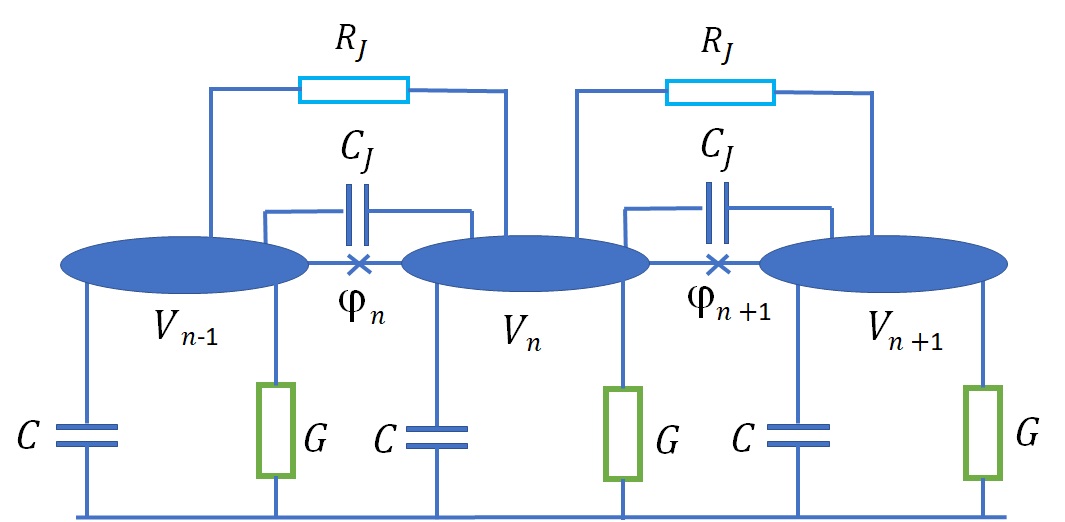
We take as the dynamical variables Josephson phases and the potentials of the grains $V_{n}$. The circuit equations are [23]

$\displaystyle\frac{\hbar}{2e}\frac{d\varphi_{n}}{dt}=V_{n-1}-V_{n},$ (1a)
$\displaystyle C\frac{dV_{n}}{dt}+GV_{n}=\partial^{2}_{n}\left(\frac{V_{n}}{R_{J}}+C_{J}\frac{dV_{n}}{dt}\right)$
$\displaystyle+I_{c}\left[\sin\left(\varphi_{n}+\varphi_{0}\right)-\sin\left(\varphi_{n+1}+\varphi_{0}\right)\right].$ (1b)

where $C$ is the ground capacitance, $I_{c}$ is the critical current of the JJ, $G$ is the conductance of the ohmic resistor shunting the ground capacitor, $R_{J}$ is the ohmic resistor shunting the JJ; the second-order discrete differential operator $\partial^{2}_{n}$ is defined as $\partial^{2}_{n}f_{n}\equiv f_{n-1}-2f_{n}+f_{n+1}$. For the sake of generality we consider d.c. background Josephson current $I_{c}\sin\left(\varphi_{0}\right)$ flowing along the JTL, where $\varphi_{0}$ is the d.c. Josephson phase.

Inclusion of the capacitance in parallel to the Josephson elements (inter-island capacitance) would certainly make the model more physically realistic. However it complicates the mathematics (there appears the fourth order derivative in the final equation). In spite of this the parallel capacitance was included in our previous paper dealing with parametric amplification in the JTL in the continuum approximation [23]. It turned out that such generalization of the model doesn’t lead to any qualitative differences. So in the present paper we decided to give the priority to simplicity over generality.

We can exclude $V_{n}$ and obtain closed equation for $\varphi_{n}$

$\displaystyle\frac{d^{2}\varphi_{n}}{d\tau^{2}}+Z_{J}G\frac{d\varphi_{n}}{d\tau}$
$\displaystyle=\partial^{2}_{n}\left[\sin\left(\varphi_{n}+\varphi_{0}\right)+\frac{Z_{J}}{R_{J}}\frac{d\varphi_{n}}{d\tau}+\frac{C_{J}}{C}\frac{d^{2}\varphi_{n}}{d\tau^{2}}\right],$ (2)

where we introduced the dimensionless time $\tau=t/\sqrt{L_{J}C}$, $Z_{J}\equiv\sqrt{L_{J}/C}$ is the characteristic impedance of the JTL, and $L_{J}=\hbar/(2eI_{c})$. Let us present (II) as

$\displaystyle\frac{d^{2}\varphi_{n}}{d\tau^{2}}-\partial_{n}^{2}\left(\cos\varphi_{0}\cdot\varphi_{n}+\frac{C_{J}}{C}\frac{d^{2}\varphi_{n}}{d\tau^{2}}\right)$
$\displaystyle=\partial_{n}^{2}\left\{\frac{Z_{J}}{R_{J}}\frac{d\varphi_{n}}{d\tau}+n.l.[\sin\left(\varphi_{n}+\varphi_{0}\right)]\right\}-Z_{J}G\frac{d\varphi_{n}}{d\tau},$ (3)

where n.l. stands for the non-linear terms of expansion of the sine function in Taylor series.

If we ignore the dissipation and the non-linear terms, Eq. (II) has obvious solution

$\displaystyle\varphi_{n}=\frac{1}{2}\sum_{\alpha}A_{\alpha}e^{i(k_{\alpha}n-\omega_{\alpha}\tau)}+c.c.,$ (4)

where

$\displaystyle\omega_{\alpha}^{2}=\frac{4\cos\varphi_{0}\sin^{2}\left(\frac{k_{\alpha}}{2}\right)}{1+\frac{4C_{J}}{C}\sin^{2}\left(\frac{k_{\alpha}}{2}\right)},$ (5)

and $A_{\alpha}$ are arbitrary constant amplitudes. The nonlinearity and the dissipation we’ll take into account approximately, by changing (4) to

$\displaystyle\varphi_{n}=\frac{1}{2}\sum_{\alpha}A_{\alpha}(n)e^{i(k_{\alpha}n-\omega_{\alpha}\tau)}+c.c.$ (6)

and assuming that the complex amplitudes $A_{\alpha}(n)$ slowly change with $n$. Additionally, because we consider the dissipation and nonlinear terms as being in some sense small, while calculating the discrete second order derivative of the terms in the parenthesis in (II) we will ignore the corrections which come from the $n$-dependence of the amplitudes, thus the discrete second derivative operator acting on a partial wave with the wave vector $k$ just multiplies this partial wave by $-4\sin^{2}\left(\frac{k}{2}\right)$. For example,

$\displaystyle\frac{d}{d\tau}\left(\varphi_{n-1}-2\varphi_{n}-\varphi_{n+1}\right)$
$\displaystyle=-2i\sum_{\alpha}\sin^{2}\left(\frac{k_{\alpha}}{2}\right)\omega_{\alpha}A_{\alpha}e^{i(k_{\alpha}n-\omega_{\alpha}\tau)}+c.c.,$ (7)

However, we’ll do better while calculating the discrete second derivative standing in the l.h.s. of (II). We promote $n$, as argument of the amplitudes, to the continuous variable $Z$ and approximate

$\displaystyle A_{\alpha}(n\pm 1)=A_{\alpha}(Z)\pm\frac{\partial A_{\alpha}(Z)}{\partial Z}.$ (8)

As the result, for the discrete second derivative we obtain

$\displaystyle\varphi_{n-1}-2\varphi_{n}+\varphi_{n+1}$
$\displaystyle=-2\sum_{\alpha}\sin^{2}\left(\frac{k_{\alpha}}{2}\right)A_{\alpha}e^{i(\omega_{\alpha}\tau-k_{\alpha}n)}+c.c.,$
$\displaystyle+i\sum_{\alpha}\sin(k_{\alpha})\frac{\partial A_{\alpha}}{\partial Z}e^{i(k_{\alpha}n-\omega_{\alpha}\tau)}+c.c.$ (9)

III 3 waves mixing

III-A Coupled equations for the amplitudes

Now let us take into account the nonlinear terms. Consider the case $\varphi_{0}\sim 1$ and $\left|\varphi_{n}\right|\ll 1$ Expanding the sine function in the r.h.s. of (II) in Taylor series and keeping the first two terms of the expansion we have

$\displaystyle n.l.\left[\sin\left(\varphi_{n}+\varphi_{0}\right)\right]=-\frac{\sin\varphi_{0}}{2}\varphi_{n}^{2}.$ (10)

After we substitute (4) into (10), the general result for the quadratic term would be too complicated, so we’ll consider a superposition of only three waves (pump, signal, and idler), with the frequencies $\omega_{p}$, Ο‰ssubscriptπœ”π‘ \omega_{s} and $\omega_{i}$ respectively, satisfying equation

Ο‰s+Ο‰i=Ο‰p.subscriptπœ”π‘ subscriptπœ”π‘–subscriptπœ”π‘\displaystyle\omega_{s}+\omega_{i}=\omega_{p}. (11)

Keeping only the terms which have Ο‰p,s,i​tsubscriptπœ”π‘π‘ π‘–π‘‘\omega_{p,s,i}t time dependence we obtain

Ο†n2=12​As​Ai​ei​[(ks+ki)​nβˆ’Ο‰p​t]+12​Ap​Aiβˆ—β€‹ei​[(kpβˆ’ki)​nβˆ’Ο‰s​t]superscriptsubscriptπœ‘π‘›212subscript𝐴𝑠subscript𝐴𝑖superscript𝑒𝑖delimited-[]subscriptπ‘˜π‘ subscriptπ‘˜π‘–π‘›subscriptπœ”π‘π‘‘12subscript𝐴𝑝superscriptsubscript𝐴𝑖superscript𝑒𝑖delimited-[]subscriptπ‘˜π‘subscriptπ‘˜π‘–π‘›subscriptπœ”π‘ π‘‘\displaystyle\varphi_{n}^{2}=\frac{1}{2}A_{s}A_{i}e^{i[(k_{s}+k_{i})n-\omega_{p}t]}+\frac{1}{2}A_{p}A_{i}^{*}e^{i[(k_{p}-k_{i})n-\omega_{s}t]}
+12​Ap​Asβˆ—β€‹ei​[(kpβˆ’ks)​nβˆ’Ο‰i​t]+c.c.formulae-sequence12subscript𝐴𝑝superscriptsubscript𝐴𝑠superscript𝑒𝑖delimited-[]subscriptπ‘˜π‘subscriptπ‘˜π‘ π‘›subscriptπœ”π‘–π‘‘π‘π‘\displaystyle+\frac{1}{2}A_{p}A_{s}^{*}e^{i[(k_{p}-k_{s})n-\omega_{i}t]}+c.c. (12)

Finally, collective all the perturbative terms in (II) we obtain coupled equations for the amplitudes

$\displaystyle\frac{dA_{p}}{dZ}+\nu_{p}A_{p}$ $\displaystyle=i\mu_{p}A_{s}A_{i}e^{i\Delta k\cdot Z}$ (13a)
d​As,id​Z+Ξ½s​As,i𝑑subscript𝐴𝑠𝑖𝑑𝑍subscriptπœˆπ‘ subscript𝐴𝑠𝑖\displaystyle\frac{dA_{s,i}}{dZ}+\nu_{s}A_{s,i} =i​μs,i​Ap​Ai,sβˆ—β€‹eβˆ’i​Δ​kβ‹…Z,absent𝑖subscriptπœ‡π‘ π‘–subscript𝐴𝑝superscriptsubscript𝐴𝑖𝑠superscriptπ‘’β‹…π‘–Ξ”π‘˜π‘\displaystyle=i\mu_{s,i}A_{p}A_{i,s}^{*}e^{-i\Delta k\cdot Z}, (13b)

where

$\displaystyle\nu_{\alpha}$ $\displaystyle=\frac{\tan(k_{\alpha}/2)}{\omega_{\alpha}}\left[Z_{J}G+4\sin^{2}\left(\frac{k_{\alpha}}{2}\right)\frac{Z_{J}}{R_{J}}\right]$ (14a)
$\displaystyle\mu_{p}$ =2​sin⁑φ0β‹…tan⁑(kp/2)Ο‰p2​sin2⁑(ks+ki2)absentβ‹…2subscriptπœ‘0subscriptπ‘˜π‘2superscriptsubscriptπœ”π‘2superscript2subscriptπ‘˜π‘ subscriptπ‘˜π‘–2\displaystyle=\frac{2\sin\varphi_{0}\cdot\tan(k_{p}/2)}{\omega_{p}^{2}}\sin^{2}\left(\frac{k_{s}+k_{i}}{2}\right) (14b)
ΞΌs,isubscriptπœ‡π‘ π‘–\displaystyle\mu_{s,i} =2​sin⁑φ0β‹…tan⁑(ks,i/2)Ο‰s,i2​sin2⁑(kpβˆ’ki,s2)absentβ‹…2subscriptπœ‘0subscriptπ‘˜π‘ π‘–2superscriptsubscriptπœ”π‘ π‘–2superscript2subscriptπ‘˜π‘subscriptπ‘˜π‘–π‘ 2\displaystyle=\frac{2\sin\varphi_{0}\cdot\tan(k_{s,i}/2)}{\omega_{s,i}^{2}}\sin^{2}\left(\frac{k_{p}-k_{i,s}}{2}\right) (14c)
$\displaystyle\Delta k$ =ks+kiβˆ’kp.absentsubscriptπ‘˜π‘ subscriptπ‘˜π‘–subscriptπ‘˜π‘\displaystyle=k_{s}+k_{i}-k_{p}. (14d)

Comparing Eqs. (13) with the appropriate equations from our previous publication [23], we see that the basic equations systems in the discrete consideration and in continuum approximation are the same. Only the parameters of the systems are different (compare (14) with the appropriate equations from our previous publication [23]).

III-B Weak signal: threshold for the parametric amplification

Let us solve Eq. (13) in the small (relative to the pump) signal and idler approximation ($|A_{s}|,|A_{i}|\ll|A_{p}|$). In this approximation the equation for $A_{p}$ becomes decoupled from the other two and takes the form

$\displaystyle\frac{dA_{p}}{dZ}+\nu_{p}A_{p}=0,$ (15)

with the obvious solution

$\displaystyle A_{p}(Z)=e^{-\nu_{p}Z}A_{p}^{0}.$ (16)

Treating the other two equations, we’ll introduce the local approximation, by treating $A_{p}$ in the r.h.s. of Eqs. (13b) as a constant. In this approximation the solutions for $A_{s},A_{i}$ are

$\displaystyle\left(\begin{array}[]{c}A_{s}\\ A_{i}\end{array}\right)=e^{-i\Delta k/2\cdot Z}\left(\begin{array}[]{c}\dots e^{KZ}\\ \dots e^{K^{*}Z}\end{array}\right),$ (21)

where dots stand for some constant amplitudes, and $K$ is one of the roots of the characteristic polynomial

P​(K)≑K2+(Ξ½s+Ξ½i)​K𝑃𝐾superscript𝐾2subscriptπœˆπ‘ subscriptπœˆπ‘–πΎ\displaystyle P(K)\equiv K^{2}+(\nu_{s}+\nu_{i})K
+(Ξ½sβˆ’i​Δ​k/2)​(Ξ½i+i​Δ​k/2)βˆ’ΞΌs​μi​|Ap|2.subscriptπœˆπ‘ π‘–Ξ”π‘˜2subscriptπœˆπ‘–π‘–Ξ”π‘˜2subscriptπœ‡π‘ subscriptπœ‡π‘–superscriptsubscript𝐴𝑝2\displaystyle+(\nu_{s}-i\Delta k/2)(\nu_{i}+i\Delta k/2)-\mu_{s}\mu_{i}\left|A_{p}\right|^{2}. (22)

Parametric amplification of the signal takes place when one of the roots have positive real part. The boundary between the parametric amplification and no parametric amplification we can find by demanding that $K$ for that boundary is purely imaginary. So, after simple algebra, we obtain the condition for the parametric amplification:

ΞΌs​μi​|Ap|2>Ξ½s​νp​[1+(Δ​k)2(Ξ½s+Ξ½i)2].subscriptπœ‡π‘ subscriptπœ‡π‘–superscriptsubscript𝐴𝑝2subscriptπœˆπ‘ subscriptπœˆπ‘delimited-[]1superscriptΞ”π‘˜2superscriptsubscriptπœˆπ‘ subscriptπœˆπ‘–2\displaystyle\mu_{s}\mu_{i}\left|A_{p}\right|^{2}>\nu_{s}\nu_{p}\left[1+\frac{\left(\Delta k\right)^{2}}{(\nu_{s}+\nu_{i})^{2}}\right]. (23)

Looking at Eq. (23) we realise that the momenta mismatch $\Delta k$ acts in some sense similar to the losses in the system. Both factors together define the threshold for the parametric amplification.

Though it’s not completely consistent, we bring back the coordinate dependence of $A_{p}$, given by Eq. (16), and consider (23) as a local condition for the parametric amplification.

III-C Small wave vectors limiting case

Consider the limiting case kp,ks,kiβ‰ͺ1much-less-thansubscriptπ‘˜π‘subscriptπ‘˜π‘ subscriptπ‘˜π‘–1k_{p},k_{s},k_{i}\ll 1. In this case $\Delta k=0$. We assume additionally that $R_{J}=\infty$, hence $\nu_{\alpha}=\nu$ (doesn’t depend upon $\alpha$). Hence Eqs. (13a), (13b) take the form

$\displaystyle\frac{dA_{p}}{dZ}+\nu A_{p}$ $\displaystyle=i\mu_{p}A_{s}A_{i}$ (24a)
d​As,id​Z+ν​As,i𝑑subscriptπ΄π‘ π‘–π‘‘π‘πœˆsubscript𝐴𝑠𝑖\displaystyle\frac{dA_{s,i}}{dZ}+\nu A_{s,i} =i​μs,i​Ap​Ai,sβˆ—,absent𝑖subscriptπœ‡π‘ π‘–subscript𝐴𝑝superscriptsubscript𝐴𝑖𝑠\displaystyle=i\mu_{s,i}A_{p}A_{i,s}^{*}, (24b)

where

ΞΌp=ΞΌs+ΞΌi.subscriptπœ‡π‘subscriptπœ‡π‘ subscriptπœ‡π‘–\displaystyle\mu_{p}=\mu_{s}+\mu_{i}. (25)

We’ll present the amplitudes as

Ap=i​eβˆ’Ξ½β€‹Z​Ap(r),As,i=eβˆ’Ξ½β€‹Z​As,i(r).formulae-sequencesubscript𝐴𝑝𝑖superscriptπ‘’πœˆπ‘superscriptsubscriptπ΄π‘π‘Ÿsubscript𝐴𝑠𝑖superscriptπ‘’πœˆπ‘superscriptsubscriptπ΄π‘ π‘–π‘Ÿ\displaystyle A_{p}=ie^{-\nu Z}A_{p}^{(r)},\hskip 14.22636ptA_{s,i}=e^{-\nu Z}A_{s,i}^{(r)}. (26)

In the new variables Eqs. (24a), (24b) take the form (compare with Ref. [24])

$\displaystyle\frac{dA_{p}^{(r)}}{d\tilde{Z}}$ =ΞΌp​As(r)​Ai(r)absentsubscriptπœ‡π‘superscriptsubscriptπ΄π‘ π‘Ÿsuperscriptsubscriptπ΄π‘–π‘Ÿ\displaystyle=\mu_{p}A_{s}^{(r)}A_{i}^{(r)} (27a)
d​As,i(r)d​Z~𝑑superscriptsubscriptπ΄π‘ π‘–π‘Ÿπ‘‘~𝑍\displaystyle\frac{dA_{s,i}^{(r)}}{d\tilde{Z}} =βˆ’ΞΌs,i​Ap(r)​Ai,s(r),absentsubscriptπœ‡π‘ π‘–superscriptsubscriptπ΄π‘π‘Ÿsuperscriptsubscriptπ΄π‘–π‘ π‘Ÿ\displaystyle=-\mu_{s,i}A_{p}^{(r)}A_{i,s}^{(r)}, (27b)

where

$\displaystyle d\tilde{Z}\equiv e^{-\nu Z}dZ,$ (28)

that is

$\displaystyle\tilde{Z}=K-\frac{1}{\nu}e^{-\nu Z},$ (29)

where $K$ is an arbitrary constant.

We’ll consider only the real solutions, postponing the general analysis until later. From (27a), (27b) follows

12​dd​Z~​[Ap(r)2+As(r)2+Ai(r)2]12𝑑𝑑~𝑍delimited-[]superscriptsubscriptsuperscriptπ΄π‘Ÿπ‘2superscriptsubscriptsuperscriptπ΄π‘Ÿπ‘ 2superscriptsubscriptsuperscriptπ΄π‘Ÿπ‘–2\displaystyle\frac{1}{2}\frac{d}{d\tilde{Z}}\left[{A^{(r)}_{p}}^{2}+{A^{(r)}_{s}}^{2}+{A^{(r)}_{i}}^{2}\right]
=(ΞΌpβˆ’ΞΌsβˆ’ΞΌi)​Ap(r)​As(r)​Ai(r).absentsubscriptπœ‡π‘subscriptπœ‡π‘ subscriptπœ‡π‘–superscriptsubscriptπ΄π‘π‘Ÿsuperscriptsubscriptπ΄π‘ π‘Ÿsuperscriptsubscriptπ΄π‘–π‘Ÿ\displaystyle=\left(\mu_{p}-\mu_{s}-\mu_{i}\right)A_{p}^{(r)}A_{s}^{(r)}A_{i}^{(r)}. (30)

Due to (25) the r.h.s. of (III-C) is equal to zero, hence

Ap(r)2+As(r)2+Ai(r)2=const,superscriptsubscriptsuperscriptπ΄π‘Ÿπ‘2superscriptsubscriptsuperscriptπ΄π‘Ÿπ‘ 2superscriptsubscriptsuperscriptπ΄π‘Ÿπ‘–2const\displaystyle{A^{(r)}_{p}}^{2}+{A^{(r)}_{s}}^{2}+{A^{(r)}_{i}}^{2}=\text{const}, (31)

and we can look for a solution in the form (remember the spherical coordinates)

$\displaystyle A_{p}^{(r)}$ $\displaystyle=B\cos\theta$ (32a)
As(r)superscriptsubscriptπ΄π‘ π‘Ÿ\displaystyle A_{s}^{(r)} $\displaystyle=B\sin\theta\cos\phi$ (32b)
$\displaystyle A_{i}^{(r)}$ $\displaystyle=B\sin\theta\sin\phi,$ (32c)

where $B$ is an arbitrary amplitude. For the new variables $\theta$ and $\phi$ we obtain equations

$\displaystyle\frac{d\theta}{d\tilde{Z}}$ $\displaystyle=-\frac{B}{2}\mu_{p}\sin\theta\sin 2\phi$ (33a)
$\displaystyle\frac{d\phi}{d\tilde{Z}}$ =βˆ’B2​cos⁑θ​(ΞΌp​cos⁑2β€‹Ο•βˆ’ΞΌs+ΞΌi).absent𝐡2πœƒsubscriptπœ‡π‘2italic-Ο•subscriptπœ‡π‘ subscriptπœ‡π‘–\displaystyle=-\frac{B}{2}\cos\theta\left(\mu_{p}\cos 2\phi-\mu_{s}+\mu_{i}\right). (33b)

Dividing one of the equations to the other we obtain

d​θtan⁑θ=ΞΌp​sin⁑2​ϕ​d​ϕμp​cos⁑2β€‹Ο•βˆ’ΞΌs+ΞΌi.π‘‘πœƒπœƒsubscriptπœ‡π‘2italic-ϕ𝑑italic-Ο•subscriptπœ‡π‘2italic-Ο•subscriptπœ‡π‘ subscriptπœ‡π‘–\displaystyle\frac{d\theta}{\tan\theta}=\frac{\mu_{p}\sin 2\phi d\phi}{\mu_{p}\cos 2\phi-\mu_{s}+\mu_{i}}. (34)

Equation (34) can be easily integrated and we obtain

sin2⁑θ=DΞΌp​cos⁑2β€‹Ο•βˆ’ΞΌs+ΞΌi,superscript2πœƒπ·subscriptπœ‡π‘2italic-Ο•subscriptπœ‡π‘ subscriptπœ‡π‘–\displaystyle\sin^{2}\theta=\frac{D}{\mu_{p}\cos 2\phi-\mu_{s}+\mu_{i}}, (35)

where $D$ is the integration constant. The solution (35), plotted in the variables $A_{\alpha}^{(r)}$, is graphically presented in Fig. 2. In the variables $A_{\alpha}$ the sphere contracts uniformly.

Refer to caption
Figure 2: The solution (35) plotted in the variables $A_{\alpha}^{(r)}$. We have chosen ΞΌi/ΞΌs=1.2subscriptπœ‡π‘–subscriptπœ‡π‘ 1.2\mu_{i}/\mu_{s}=1.2 and $\theta=.1$ for $\phi=0$.

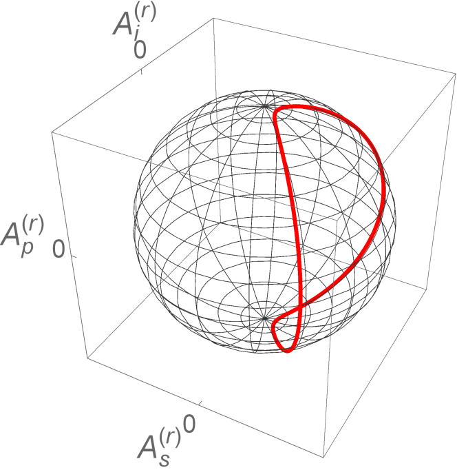
Equation (35) is even simpler than it looks.Taking into account (31), it can be written down as

(ΞΌsβˆ’ΞΌi)​Ap(r)2+ΞΌp​(As(r)2βˆ’Ai(r)2)=const.subscriptπœ‡π‘ subscriptπœ‡π‘–superscriptsuperscriptsubscriptπ΄π‘π‘Ÿ2subscriptπœ‡π‘superscriptsuperscriptsubscriptπ΄π‘ π‘Ÿ2superscriptsuperscriptsubscriptπ΄π‘–π‘Ÿ2const\displaystyle(\mu_{s}-\mu_{i}){A_{p}^{(r)}}^{2}+\mu_{p}\left({A_{s}^{(r)}}^{2}-{A_{i}^{(r)}}^{2}\right)=\text{const}. (36)

The latter equation follows immediately from (27a), (27b).

There also exists a singular solution of (33a), (33b), where the constant $\phi$ is given by the equation

ΞΌp​cos⁑2β€‹Ο•βˆ’ΞΌs+ΞΌi=0,subscriptπœ‡π‘2italic-Ο•subscriptπœ‡π‘ subscriptπœ‡π‘–0\displaystyle\mu_{p}\cos 2\phi-\mu_{s}+\mu_{i}=0, (37)

and $\theta(\tilde{Z})$, found from (33a), is given by the equation

$\displaystyle\cos\theta=\tanh\left(\frac{B}{2}\mu_{p}\sin 2\phi\cdot\tilde{Z}\right).$ (38)

Equation (38) shows that when $\tilde{Z}\to\infty$, either $\theta\to 0$ or $\theta\to\pi$, depending upon the sign of $\sin 2\phi$.

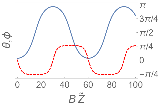
However, we are mostly interested not in the dependence of one angle variable upon the other, but in their dependence upon $\tilde{Z}$. This dependence can be found by numerical integration of Eqs. (33a), (33b) and is illustrated in Fig. 3. The left side of the Figure, with $\theta$ increasing from nearly 0, to $\pi/2$, demonstrates the parametric amplification (provided the losses are not too big).

Refer to caption
Figure 3: Numerical solution of Eqs. (33a), (33b) for $\theta$ (blue solid line) and $\varphi$ (red dashed line). We have chosen ΞΌs=.2subscriptπœ‡π‘ .2\mu_{s}=.2, $\mu_{i}=.24$, $\theta(0)=.1$ and $\varphi(0)=0$ (no idle signal at $\tilde{Z}=0$).

IV 4 waves mixing

IV-A Coupled equations for the amplitudes

Now let us consider the case $\varphi_{0}=0$. In this case, expanding the sine function in the r.h.s. of (II) in Taylor series with respect to phases difference and keeping the first two nonzero terms of the expansion we have

$\displaystyle n.l.\left[\sin\left(\varphi_{n}\right)\right]=-\frac{1}{6}\varphi_{n}^{3}.$ (39)

We again consider the superposition of three waves, but the frequencies this time satisfy the relation

Ο‰s+Ο‰i=2​ωp.subscriptπœ”π‘ subscriptπœ”π‘–2subscriptπœ”π‘\displaystyle\omega_{s}+\omega_{i}=2\omega_{p}. (40)

Keeping only the terms which have Ο‰p,s,i​tsubscriptπœ”π‘π‘ π‘–π‘‘\omega_{p,s,i}t time dependence we obtain

$\displaystyle\varphi_{n}^{3}=\frac{3}{8}\sum_{\alpha,\beta}\left(2-\delta_{\alpha\beta}\right)A_{\alpha}\left|A_{\beta}\right|^{2}e^{i[k_{\alpha}n-\omega_{\alpha}t]}$
+34​Apβˆ—β€‹As​Ai​ei​[(ks+kiβˆ’kp)​nβˆ’Ο‰p​t]+38​Ap2​Aiβˆ—β€‹ei​[(2​kpβˆ’ki)​nβˆ’Ο‰s​t]34superscriptsubscript𝐴𝑝subscript𝐴𝑠subscript𝐴𝑖superscript𝑒𝑖delimited-[]subscriptπ‘˜π‘ subscriptπ‘˜π‘–subscriptπ‘˜π‘π‘›subscriptπœ”π‘π‘‘38superscriptsubscript𝐴𝑝2superscriptsubscript𝐴𝑖superscript𝑒𝑖delimited-[]2subscriptπ‘˜π‘subscriptπ‘˜π‘–π‘›subscriptπœ”π‘ π‘‘\displaystyle+\frac{3}{4}A_{p}^{*}A_{s}A_{i}e^{i[(k_{s}+k_{i}-k_{p})n-\omega_{p}t]}+\frac{3}{8}A_{p}^{2}A_{i}^{*}e^{i[(2k_{p}-k_{i})n-\omega_{s}t]}
+38​Ap2​Asβˆ—β€‹ei​[(2​kpβˆ’ks)​nβˆ’Ο‰i​t]+c.c..formulae-sequence38superscriptsubscript𝐴𝑝2superscriptsubscript𝐴𝑠superscript𝑒𝑖delimited-[]2subscriptπ‘˜π‘subscriptπ‘˜π‘ π‘›subscriptπœ”π‘–π‘‘π‘π‘\displaystyle+\frac{3}{8}A_{p}^{2}A_{s}^{*}e^{i[(2k_{p}-k_{s})n-\omega_{i}t]}+c.c.. (41)

Finally, collective all the perturbative terms in (II) we obtain coupled equations for the amplitudes

$\displaystyle\frac{dA_{p}}{dZ}+\nu_{p}A_{p}$ $\displaystyle=i\gamma_{p}\left(|A_{p}|^{2}+2|A_{s}|^{2}+2|A_{i}|^{2}\right)A_{p}$
$\displaystyle+2i\eta_{p}A_{p}^{*}A_{s}A_{i}e^{i\Delta k\cdot Z}$ (42a)
d​As,id​Z+Ξ½s,i​As,i𝑑subscript𝐴𝑠𝑖𝑑𝑍subscriptπœˆπ‘ π‘–subscript𝐴𝑠𝑖\displaystyle\frac{dA_{s,i}}{dZ}+\nu_{s,i}A_{s,i} $\displaystyle=i\gamma_{s,i}\left(2|A_{p}|^{2}+|A_{s,i}|^{2}+2|A_{i,s}|^{2}\right)A_{s,i}$
+i​ηs,i​Ap2​Ai,sβˆ—β€‹eβˆ’i​Δ​kβ‹…Z,𝑖subscriptπœ‚π‘ π‘–superscriptsubscript𝐴𝑝2superscriptsubscript𝐴𝑖𝑠superscriptπ‘’β‹…π‘–Ξ”π‘˜π‘\displaystyle+i\eta_{s,i}A_{p}^{2}A_{i,s}^{*}e^{-i\Delta k\cdot Z}, (42b)

where $\nu_{\alpha}$ is given by (14a) with $\cos\varphi_{0}$ being put equal to 1, and

$\displaystyle\gamma_{\alpha}$ $\displaystyle=\frac{\tan(k_{\alpha}/2)}{2\omega_{\alpha}^{2}}\sin^{2}\left(\frac{k_{\alpha}}{2}\right)$ (43a)
$\displaystyle\eta_{p}$ =tan⁑(kp/2)2​ωp2​sin2⁑(ks+kiβˆ’kp2)absentsubscriptπ‘˜π‘22superscriptsubscriptπœ”π‘2superscript2subscriptπ‘˜π‘ subscriptπ‘˜π‘–subscriptπ‘˜π‘2\displaystyle=\frac{\tan(k_{p}/2)}{2\omega_{p}^{2}}\sin^{2}\left(\frac{k_{s}+k_{i}-k_{p}}{2}\right) (43b)
Ξ·s,isubscriptπœ‚π‘ π‘–\displaystyle\eta_{s,i} =tan⁑(ks,i/2)2​ωp2​sin2⁑(2​kpβˆ’ki,s2)absentsubscriptπ‘˜π‘ π‘–22superscriptsubscriptπœ”π‘2superscript22subscriptπ‘˜π‘subscriptπ‘˜π‘–π‘ 2\displaystyle=\frac{\tan(k_{s,i}/2)}{2\omega_{p}^{2}}\sin^{2}\left(\frac{2k_{p}-k_{i,s}}{2}\right) (43c)
$\displaystyle\Delta k$ =ks+kiβˆ’2​kpabsentsubscriptπ‘˜π‘ subscriptπ‘˜π‘–2subscriptπ‘˜π‘\displaystyle=k_{s}+k_{i}-2k_{p} (43d)

Comparing Eqs. (42) with the appropriate equations from our previous publication [23] we can only repeat what was said in the very end of Section III-A.

IV-B Weak signal

In the small (relative to the pump) signal and idler approximation ($|A_{s}|,|A_{i}|\ll|A_{p}|$), the equation for $A_{p}$ becomes decoupled from the other two and takes the form

$\displaystyle\frac{dA_{p}}{dZ}+\nu_{p}A_{p}=\frac{i}{2}\gamma_{p}|A_{p}|^{2}A_{p}.$ (44)

It is interesting to compare the result following from equation (44) with the nonlinear dispersion law obtained in our previous publication [25]. There we considered equation

$\displaystyle\frac{d^{2}\varphi_{n}}{d\tau^{2}}=\sin\varphi_{n-1}-2\sin\varphi_{n}+\sin\varphi_{n+1}$ (45)

and obtained in the up to the second order with respect to the amplitude approximation the solution

$\displaystyle\varphi_{n}(\tau)=a\cos[kn-\omega(k)\tau]$ (46)

with the dispersion law

$\displaystyle\omega(k)=2\left(1-\frac{a^{2}}{16}\right)\sin\left(\frac{k}{2}\right).$ (47)

In the absence of dissipation, the solution of (44) can be taken as

$\displaystyle A_{p}(Z)=ae^{i\gamma_{p}a^{2}/2Z},$ (48)

where $a$ is a real constant. Substituting this solution into (6) and taking into account (43a) we obtain

$\displaystyle\varphi_{n}(\tau)=a\cos[(k+a^{2}\tan(k/2)/8)n-\omega\tau],$ (49)

where $\omega=2\sin(k/2)$. let us introduce

$\displaystyle k^{\prime}=k+a^{2}\tan(k/2)/8.$ (50)

Then up to the lowest order with respect to $a^{2}$ corrections

$\displaystyle k=k^{\prime}-a^{2}\tan(k^{\prime}/2)/8,$ (51)

and the dispersion law can be presented as

$\displaystyle\omega=2\sin[k^{\prime}/2-a^{2}\tan(k^{\prime}/2)/16].$ (52)

Expanding (52) in series with respect to $a^{2}$ and keeping the terms up to the linear order with respect to $a^{2}$ we obtain

$\displaystyle\omega(k^{\prime})=2\left(1-\frac{a^{2}}{16}\right)\sin\left(\frac{k^{\prime}}{2}\right).$ (53)

which coincides with Eq. (47).

Note that in our previous publications [25] the pump wave hire harmonics, which exist simultaneously with the main one, due to nonlinearity of the system, are also considered. However there influence on the signal amplitude would be an effect of the higher order with respect to the parameter $A_{p}^{2}$, than the influence of the main harmonic.

IV-C Threshold for the parametric amplification

Equations (42b) in the weak signal approximation can be written down as

d​As,id​Z+(Ξ½s,iβˆ’i​γs,i​|Ap|2)​As,i=i​ηs,i​Ap2​Ai,sβˆ—β€‹eβˆ’i​Δ​kβ‹…Z.𝑑subscript𝐴𝑠𝑖𝑑𝑍subscriptπœˆπ‘ π‘–π‘–subscript𝛾𝑠𝑖superscriptsubscript𝐴𝑝2subscript𝐴𝑠𝑖𝑖subscriptπœ‚π‘ π‘–superscriptsubscript𝐴𝑝2superscriptsubscript𝐴𝑖𝑠superscriptπ‘’β‹…π‘–Ξ”π‘˜π‘\displaystyle\frac{dA_{s,i}}{dZ}+\left(\nu_{s,i}-i\gamma_{s,i}|A_{p}|^{2}\right)A_{s,i}=i\eta_{s,i}A_{p}^{2}A_{i,s}^{*}e^{-i\Delta k\cdot Z}. (54)

In the framework of the local approximation, we treat $A_{p}$ in the r.h.s. of Eqs. (54) as a constant, so we recover (21), where $K$ this time is one of the roots of the characteristic polynomial

P​(K)≑K2+(Ξ½s+Ξ½i)​K+(Ξ½sβˆ’2​i​γs​|Ap|2βˆ’i​Δ​k/2)𝑃𝐾superscript𝐾2subscriptπœˆπ‘ subscriptπœˆπ‘–πΎsubscriptπœˆπ‘ 2𝑖subscript𝛾𝑠superscriptsubscript𝐴𝑝2π‘–Ξ”π‘˜2\displaystyle P(K)\equiv K^{2}+(\nu_{s}+\nu_{i})K+(\nu_{s}-2i\gamma_{s}|A_{p}|^{2}-i\Delta k/2)
β‹…(Ξ½i+2​i​γi​|Ap|2+i​Δ​k/2)βˆ’Ξ·s​ηi​|Ap|4.β‹…absentsubscriptπœˆπ‘–2𝑖subscript𝛾𝑖superscriptsubscript𝐴𝑝2π‘–Ξ”π‘˜2subscriptπœ‚π‘ subscriptπœ‚π‘–superscriptsubscript𝐴𝑝4\displaystyle\cdot(\nu_{i}+2i\gamma_{i}|A_{p}|^{2}+i\Delta k/2)-\eta_{s}\eta_{i}\left|A_{p}\right|^{4}. (55)

We again find the boundary between the parametric amplification and no amplification by demanding that $K$ for that boundary is purely imaginary. So, after simple algebra, we obtain the condition for the parametric amplification:

Ξ·s​ηi​|Ap|4>Ξ½s​νi​{1+[Δ​k+2​(Ξ³s+Ξ³i)​|Ap|2]2(Ξ½s+Ξ½i)2}.subscriptπœ‚π‘ subscriptπœ‚π‘–superscriptsubscript𝐴𝑝4subscriptπœˆπ‘ subscriptπœˆπ‘–1superscriptdelimited-[]Ξ”π‘˜2subscript𝛾𝑠subscript𝛾𝑖superscriptsubscript𝐴𝑝22superscriptsubscriptπœˆπ‘ subscriptπœˆπ‘–2\displaystyle\eta_{s}\eta_{i}\left|A_{p}\right|^{4}>\nu_{s}\nu_{i}\left\{1+\frac{\left[\Delta k+2(\gamma_{s}+\gamma_{i})\left|A_{p}\right|^{2}\right]^{2}}{(\nu_{s}+\nu_{i})^{2}}\right\}. (56)

Here we can only repeat what was said after Eq. (23). Again, we bring back the coordinate dependence of $A_{p}$, given by Eq. (44) and consider (56) as a local condition for the parametric amplification.

V Discussion

The present paper generalized the previously obtained results on parametric amplification in JTL [5, 11, 25] to the discrete model of the line. The discrete character of the line leads to the renormalization of the parameters of the coupled amplitude equations.

We formulate the local approximation which allows explicitly find the threshold for parametric amplification in the case of weak signal. In addition we present the exact particular solution for the coupled equations for the pump, signal and idler amplitudes in the particular case of small wave vectors and present the solution graphically. Finally, we would like to mention that in real case of the line of finite length, the frequency dependence of the line impedance leads to matching problems and hence to the wave reflection (e.g., [26]). However we leave the study of the problem until later.

Acknowledgment

I am grateful to T. H. A. van der Reep for the discussion. I am also very grateful to Donostia International Physics Center (DIPC) for the hospitality during my visit, when the paper was finalised.

References

  • [1] M. A. Castellanos-Beltran and K. W. Lehnert, Appl. Phys. Lett. 91, 083509 (2007).
  • [2] P. D. Nation, J. R. Johansson, M. P. Blencowe, and F. Nori, Rev. Mod. Phys. 84, 1 (2012).
  • [3] B. H. Eom, P. K. Day, H. G. LeDuc, and J. Zmuidzinas, Nat. Phys. 8, 623 (2012).
  • [4] J. Aumentado, IEEE Microwave magazine, 21, 45 (2020).
  • [5] O. Yaakobi, L. Friedland, C. Macklin, and I. Siddiqi, Phys. Rev. B 87, 144301 (2013).
  • [6] K. O’Brien, C. Macklin, I. Siddiqi, and X. Zhang, Phys. Rev. Lett. 113, 157001 (2014).
  • [7] C. Macklin, K. O’Brien, D. Hover, M. E. Schwartz, V. Bolkhovsky, X. Zhang, W. D. Oliver, and I. Siddiqi, Science 350, 307 (2015).
  • [8] B. A. Kochetov, and A. Fedorov, Phys. Rev. B. 92, 224304 (2015).
  • [9] M.T. Bell and A. Samolov, Phys. Rev. Applied 4, 024014 (2015).
  • [10] T. C. White et al., Appl. Phys. Lett. 106, 242601 (2015).
  • [11] A. B. Zorin, Phys. Rev. Applied 6, 034006 (2016).
  • [12] L. Fasolo, A. Greco, E. Enrico, J. Thirumalai, and S. I. Pokutnyi, Adv. Condensed - Matter Materials Physics - Rudimentary Res. Topical Technol. IntechOpen, 2019.
  • [13] D. M. Basko, F. Pfeiffer, P. Adamus, M. Holzmann, and F. W. J. Hekking, Phys. Rev. B 101, 024518 (2020).
  • [14] T. Dixon, J. W. Dunstan, G. B. Long, J. M. Williams, Ph. J. Meeson, C. D. Shelly, Phys. Rev. Applied 14, 034058 (2020)
  • [15] A. B. Zorin, Phys. Rev. Applied 12, 044051 (2019).
  • [16] A. Miano and O. A. Mukhanov, IEEE Trans. Appl. Supercond. 29, 1501706 (2019).
  • [17] T. H. A. van der Reep, Phys. Rev. A 99, 063838 (2019).
  • [18] Ch. Liu, Tzu-Chiao Chien, M. Hatridge, D. Pekker, Phys. Rev. A 101, 042323 (2020).
  • [19] A. Greco, L. Fasolo, A. Meda, L. Callegaro,and E. Enrico, Phys. Rev. B, 104, 184517 (2021).
  • [20] Y. Yuan, M. Haider, J. A. Russer, P. Russer, and Ch. Jirauschek. In European Quantum Electronics Conference, 22, Optical Society of America (2021).
  • [21] C. Kow, V. Podolskiy, and A. Kamal, arXiv:2201.04660.
  • [22] H. Katayama, N. Hatakenaka, T. Fujii, and M. P. Blencowe, Phys. Rev. Res. 5, L022055 (2023).
  • [23] E. Kogan, Phys. Stat. Sol. (b), Vol. 260, p. 2300005, 2023.
  • [24] A. L. Cullen, Proceedings of the IEE-Part B: Electronic and Communication Engineering 107, 101 (1960).
  • [25] E. Kogan, Phys. Stat. Sol. (b), Vol. 259, p. 2200160, 2022.
  • [26] S. Kern, P. Neilinger, E. Il’ichev, et al., arXiv: 2203.02448v2 (2023).