Inference of the optical depth to reionization $\tau$ from Planck CMB maps with convolutional neural networks

The optical depth to reionization, $\tau$, is the least constrained parameter of the cosmological $\Lambda$CDM model. To date, its most precise value is inferred from large-scale polarized CMB power spectra from the high-frequency instrument (HFI) aboard the Planck satellite. These maps are known to contain significant contamination by residual non-Gaussian systematic effects, which are hard to model analytically. Therefore, robust constraints on $\tau$ are currently obtained through an empirical cross-spectrum likelihood built from simulations.
In this paper, we present a likelihood-free inference of $\tau$ from polarized Planck HFI maps which, for the first time, is fully based on neural networks (NNs). NNs have the advantage of not requiring an analytical description of the data and can be trained on state-of-the-art simulations, combining the information from multiple channels.
By using Gaussian sky simulations and Planck SRoll2 simulations, including CMB, noise, and residual instrumental systematic effects, we train, test, and validate NN models considering different setups. We infer the value of $\tau$ directly from Stokes $Q$ and $U$ maps at $\sim 4^{\circ}$ pixel resolution, without computing angular power spectra.
On Planck data, we obtain $\tau_{\rm NN}=0.0579\pm 0.0082$, compatible with current $EE$ cross-spectrum results but with a $\sim 30\%$ larger uncertainty, which can be assigned to the inherent non-optimality of our estimator and to the retraining procedure applied to avoid biases.
While this paper does not improve on current cosmological constraints on $\tau$, our analysis represents a first robust application of NN-based inference on real data, and highlights its potential as a promising tool for complementary analysis of near-future CMB experiments, also in view of the ongoing challenge to achieve the first detection of primordial gravitational waves.

1 Introduction

Cosmic reionization, the period in cosmic history that accompanies the ignition of the first stars, is of great interest to both astrophysics and cosmology. At recombination, about 380,000 years after the Big Bang, free electrons were bound in hydrogen atoms, causing the decoupling of matter from the photon field that we observe today as the Cosmic Microwave Background (CMB). This is when the Universe entered the electrically neutral phase, called cosmic “dark ages”. It is presumed that about 200 million years after, cold hydrogen gas had collapsed gravitationally in dark matter halos, forming the first stars. These earliest compact sources of UV radiation heated up the surrounding hydrogen gas, progressively ionizing the whole Universe via bubbles of expanding HII regions. The first experimental evidence for reionization was the discovery of the so-called Gunn-Peterson trough in the absorption spectra of high-redshift quasars Gunn & Peterson (1965); Scheuer (1965), suggesting that the Universe must have undergone an electrically neutral phase. Modern quasar measurements predict reionization to have ended by $z\sim 6$ (Fan et al., 2006; Schroeder et al., 2012; Becker et al., 2015; Villasenor et al., 2022; Dayal & Ferrara, 2018).

Reionization plays a crucial role for cosmology, too. Photons emitted during recombination have a finite probability of Compton scattering with free electrons released during reionization. For us as observers, this has two effects: firstly, less CMB photons will reach us on Earth, having to traverse an optically thick interstellar medium. Secondly, a statistically relevant fraction of CMB photons will scatter into our line of sight, carrying a nonzero net polarization. The first effect reduces the overall intensity of CMB emission (via both the unpolarized and polarized component) by a factor $\exp(-2\tau)$, where $\tau$ is the optical depth to reionization, defined as

$$\tau=\int_{t(z_{\rm CMB})}^{t_{0}}n_{\rm e}\sigma_{\rm T}\,c\,{\rm d}t^{\prime}\,.$$ (1)

Here, $z_{\rm CMB}\approx 1100$ is the time of last scattering between photons and baryons, $n_{\rm e}$ is the electron number density and $\sigma_{\rm T}$ is the Thomson scattering cross section. The second effect gives rise to secondary anisotropies in the CMB polarization, adding power at very large angular scales $\gtrsim 20^{\circ}$ (or multipoles $\ell\lesssim 10$). Only full-sky space missions have been able to measure this “reionization bump” through pixel-based and power-spectrum-based analysis methods. $EE$ and $TE$ power spectra from WMAP 9-year release yield $\tau=0.089\pm 0.014$ (Hinshaw et al., 2013), a value that later turned out to be biased high due to Galactic dust (Planck Collaboration XI, 2016; Natale et al., 2020). The Planck low-frequency instrument (LFI) polarization data at 70 GHz contain less large-scale systematics than the HFI data at 100 GHz and 143 GHz, motivating the Planck Collaboration to perform map-based analysis on LFI and $EE$ cross-spectrum analysis on HFI. The 2018 legacy release data constrain reionization to $\tau=0.063\pm 0.020$ for LFI and $0.051\pm 0.009$ for HFI (Planck Collaboration V, 2020). The cross-spectrum analysis method of Planck HFI data at 143 GHz and 100 GHz obtains the tightest constraint on $\tau$, while avoiding the bias arising from uncorrelated noise in the individual channels.

The Planck 2018 legacy polarization data products at large scales are known to be affected by residual contamination from instrumental systematic effects. At 143 GHz and 100 GHz, these are (Planck Collaboration VI, 2014; Delouis et al., 2019):

• detector-related temperature-to-polarization ($T$-to-$P$) leakage due the analog-to-digital converter nonlinearity (ADCNL),

• uncertainties on the bolometers’ polarization efficiency and detector orientation,

• foregrounds-related $T$-to-$P$ leakage due to bandpass mismatch and inaccurate foregrounds modelling,

• the time transfer function associated with heat transfer to the bolometers.

In general, these systematic effects possess non-Gaussian statistics and are expected to correlate among different channels, mainly because they are partially sourced by the temperature signal. Several updated map-making codes have been published that improve on the systematics cleaning, like SRoll2 (Delouis et al., 2019), and NPIPE (Planck Collaboration Int. LVII, 2020). The SRoll2 algorithm, an upgraded version of the Planck Collaboration’s SRoll algorithm (Planck Collaboration Int. XLVI, 2016), iteratively cleans systematics from Planck’s time-ordered data products. Major improvements in SRoll2 encompass a new gain calibration model that accounts for second-order ADCNL, updated foreground templates, and an internal marginalization over the polarization angles and efficiencies for each bolometer. The SRoll2 data products contain a significantly lower level of spurious systematic effects and a dipole residual power reduced by 50% with respect to the Planck 2018 legacy data, falling below the noise level. The SRoll2 $EE$ cross-spectrum is dominated by the cosmological signal at all scales that were considered in the analysis ($2<\ell<30$).

In spite of the improved cleaning, a small residual contamination remains (mainly due to the second-order ADCNL effect), which may bias cosmological analyses. For their $100\times 143$ GHz $EE$ cross-spectrum analysis of the SRoll2 data products, Pagano et al. (2020) use an empirical likelihood built from realistic simulations (Planck Collaboration V, 2020; Gerbino et al., 2020), motivating their choice by the expected non-Gaussianity of the maps and by the difficulty to model residual systematic effects analytically. They obtain $\tau=0.0566^{+0.0053}_{-0.0062}$ from $EE$ only and $\tau=0.059\pm 0.006$ when combining with $TT$ data. Compared with the $EE$ results from the Planck 2018 legacy release ($\tau=0.051\pm 0.009$), this reduces the uncertainty by $\sim 40\%$ and increases the best-fit $\tau$ value by up to 0.9$\sigma$. More recently, de Belsunce et al. (2021) applied various likelihood approximation schemes on $EE$ cross-spectrum data from SRoll2 maps, finding results compatible with Pagano et al. (2020), though sightly larger by $0.3\sigma$.

In recent years, neural network (NN)-based approaches for undertaking likelihood-free inference underwent a rapid development in cosmology, showing potential as an alternative tool for parameter estimation that does not require the existence of an analytical description of data, but relies only on numerical simulations to train a regression model. In the general context of cosmology, a variety of machine learning (ML) techniques have been exploited and tested in recent years. Promising tools are being developed for many applications: from cosmic large-scale structure (LSS) simulations Villaescusa-Navarro et al. (2022), to CMB lensing reconstruction (Caldeira et al., 2019), kinetic SZ detection (Tanimura et al., 2022) or foreground cleaning and modelling (Jeffrey et al., 2022; Wang et al., 2022; Casas et al., 2022; Krachmalnicoff & Puglisi, 2021). NN-based inference of cosmological parameters has seen significant progress in the context of observations of the LSS, where the complexity of the cosmological and astrophysical signals, together with the difficulty in the definition of optimal summary statistics, challenge analytical methods. Up to now, this approach has been tested on simulations (see e.g., Villaescusa-Navarro et al., 2022), with applications on real data still limited in number, although leading to promising results (e.g. Fluri et al., 2019). In this context, CMB data analysis could also benefit from the application of NN-based inference, helping overcome the limitations of traditional methods. This is relevant, for example, for the estimation of parameters affecting the large angular scales, like the optical depth to reionization, critically harmed by the presence of spurious non-Gaussian signals, as outlined above.

In this paper, we show the first map-level cosmological inference on CMB data that is entirely based on convolutional neural networks (CNNs). We use CNNs to infer the optical depth to reionization $\tau$ and its statistical uncertainty from Planck multi-frequency maps on the 100 and 143 GHz channels at scales $\gtrsim 4^{\circ}$, having trained and validated our findings on the SRoll2 simulations. Using moment networks (Jeffrey & Wandelt, 2020), we infer $\tau$ and its statistical uncertainty $\sigma(\tau)$ from a single data set. In particular, we demonstrate:

1. When training the CNN on simulations with realistic, correlated Gaussian noise, we achieve unbiased estimates of $\tau$ from maps.

2. Our CNN models can effectively combine multi-frequency information, recognizing common features across channels, not only to reduce statistical uncertainties but also to diminish the impact of noise and systematic effects.

3. Training on non-Gaussian data is necessary to obtain unbiased results on the SRoll2 test simulations and Planck data. Limited by a low number of simulations that contain Planck systematics, we are forced to build a retrained model, which increases error bars on $\tau$ by $\sim 30\%$ in exchange for unbiased results.

We structure this paper as follows. The simulations and data used in this work are presented in Section 2, followed by the neural network inference method which we describe in Section 3. In order to validate this method, we apply it to a series of simulations and present the results in Section 4. The final results on the Planck SRoll2 maps are shown and discussed in Section 5. We conclude the paper in Section 6.

2 Simulations and data

The goal of our analysis is to build a NN model able to infer the value of the $\tau$ cosmological parameter having as input Planck low-resolution polarization maps. In particular, in this work we use the SRoll2 maps at 100 and 143 GHz. In order to achieve our goal we need a large number of simulations to perform NN training, testing and validation. We generate simulated maps that include CMB emission, noise and instrumental systematic effects, as well as possible spurious signals coming from our Galaxy. In this section, we describe the simulations, the data, and the sky masks needed to avoid the highly contaminated Galactic plane region.

2.1 Simulated CMB maps

Polarized CMB anisotropies, observed at the Planck noise levels, can be sufficiently well represented by a spin-2 field with Gaussian statistics (Planck Collaboration IX, 2020). The $TT$, $TE$ and $EE$ power spectra characterize the probability distribution of CMB temperature and polarization anisotropies and can be described by the six parameters of the $\Lambda$CDM model. Analyses of small-scale temperature data from the Planck 2018 legacy release place a $0.5\%$ constraint on the parameter combination $10^{9}\,A_{s}\,e^{-2\tau}=(1.88\pm 0.01)$ (Planck Collaboration VI, 2020). Varying the two parameters $(A_{s},\,\tau)$ simultaneously conditioned on $10^{9}\,A_{s}\,e^{-2\tau}=1.884$, we use the Boltzmann solver CAMB (Lewis et al., 2000) to generate a lookup table of $EE$ power spectra computed with the $\Lambda$CDM model. To build the simulated CMB maps used to train and validate our NN models, we discretize $\tau\in[0.01,\,0.13]$ with step size $\Delta\tau=5\times 10^{-4}$, while the other five $\Lambda$CDM parameters are fixed to the Planck 2018 legacy best-fit values $H_{0}=67.32$ km/s/Mpc, $\Omega_{b}h^{2}=0.02237$, $\Omega_{c}h^{2}=0.1201$, $n_{s}=0.9651$, $m_{\nu}=0.06$. From the tabulated power spectra we uniformly draw 200,000 samples based on which we generate 200,000 pairs of full-sky Stokes $Q$ and $U$ maps using the HEALPix package (Górski et al., 2005). We fix the $Q$ and $U$ maps’ angular pixel resolution by choosing ${N_{\rm side}}=16$ (or a pixel size of $\sim 4^{\circ}$) and smooth each map with a cosine beam window function (Benabed et al., 2009), in analogy with the procedure used to generate the Planck SRoll2 maps (see Section 2.4). These large scales retained in our maps correspond to multipoles $\ell\lesssim 50$, where the reionization peak leaves an observable imprint in the CMB $EE$ spectrum.

2.2 Simulated Gaussian noise

Planck maps contain Gaussian instrumental noise which, in pixel space, is well described by the FFP8 covariance matrices (Planck Collaboration XII, 2016). We draw samples from them for the Planck 100 and 143 GHz polarization channels (Planck Collaboration VI, 2014; Planck Collaboration XIII, 2016), obtaining 200,000 Gaussian noise maps at pixel resolution ${N_{\rm side}}=16$ for both channels, respectively. We coadd the training maps of CMB and noise to obtain 200,000 Planck-like simulations on the full sky, out of which we select 190,000 for training and 10,000 for validation. For the testing phase, we draw new noise samples in the same fashion as before, but coadd CMB simulations with fixed input values $\tau=0.05$, 0.06 and 0.07 and different seeds than the ones used for training and validation. In this way, we obtain 3 sets of 10,000 independent Gaussian test simulations with the fixed input cosmologies.

2.3 SRoll2 simulations

The SRoll2 simulations (Delouis et al., 2019) improve on the SRoll simulations published along with Planck’s third data release (Planck Collaboration Int. LVII, 2020). They are the result of applying the SRoll2 cleaning algorithm to a set of 500 Planck-like realistic sky simulations containing modeled noise, foregrounds and instrument systematics. We choose the SRoll2 simulations as our reference for systematic effects present in the SRoll2 Planck data. All simulated maps are cleaned from Galactic foregrounds through a template fitting procedure, as described in Pagano et al. (2020). In order to produce our training set, we start with 400 out of the 500 original SRoll2 simulations containing pairs of $Q$ and $U$ full-sky maps at pixel resolution ${N_{\rm side}}=16$ and two channels corresponding to 100 GHz and 143 GHz. To augment our original SRoll2 simulation set, we randomly draw SRoll2 100 GHz and 143 GHz maps from the original 400 maps (with repetition), keeping corresponding $Q$ and $U$ maps together. This allows us to assemble a total of 200,000 SRoll2 simulations. After coadding them with CMB simulations, we obtain a set of 200,000 polarized full-sky simulations, used for training and validation. For the testing phase, we make $3\times 100$ copies of $100$ unseen SRoll2 maps and coadd them with $10,000$ CMB maps with fixed input $\tau=0.05$, $0.06$ and $0.07$, respectively. In this way we obtain a set of $3\times 10,000$ full-sky SRoll2 test simulations.

2.4 Planck maps

The goal of this work is the analysis of the SRoll2 Planck polarization data products (Delouis et al., 2019). They consist of Stokes $Q$ and $U$ maps at the $100$ GHz and $143$ GHz HFI frequency channels, stored at pixel resolution ${N_{\rm side}}=16$. The Planck maps are first smoothed with cosine beam window functions, and then cleaned from foreground contamination through a template fitting procedure (Pagano et al., 2020). Figure 1 shows the map products in Galactic coordinates. We note that close to the Galactic plane, $Q$ and $U$ on both channels are visibly contaminated by residual systematic effects, which we mask prior to the analysis in order to avoid bias. The arc-shaped features in the northern and southern Galactic hemisphere likely indicate residual gain variations caused by the ADCNL systematic effect. As shown by Delouis et al. (2019), these features show lower residual power than the CMB in the 100$\times$143 GHz $EE$ cross-spectrum, but may still amount to a non-negligible bias in cosmological analyses.

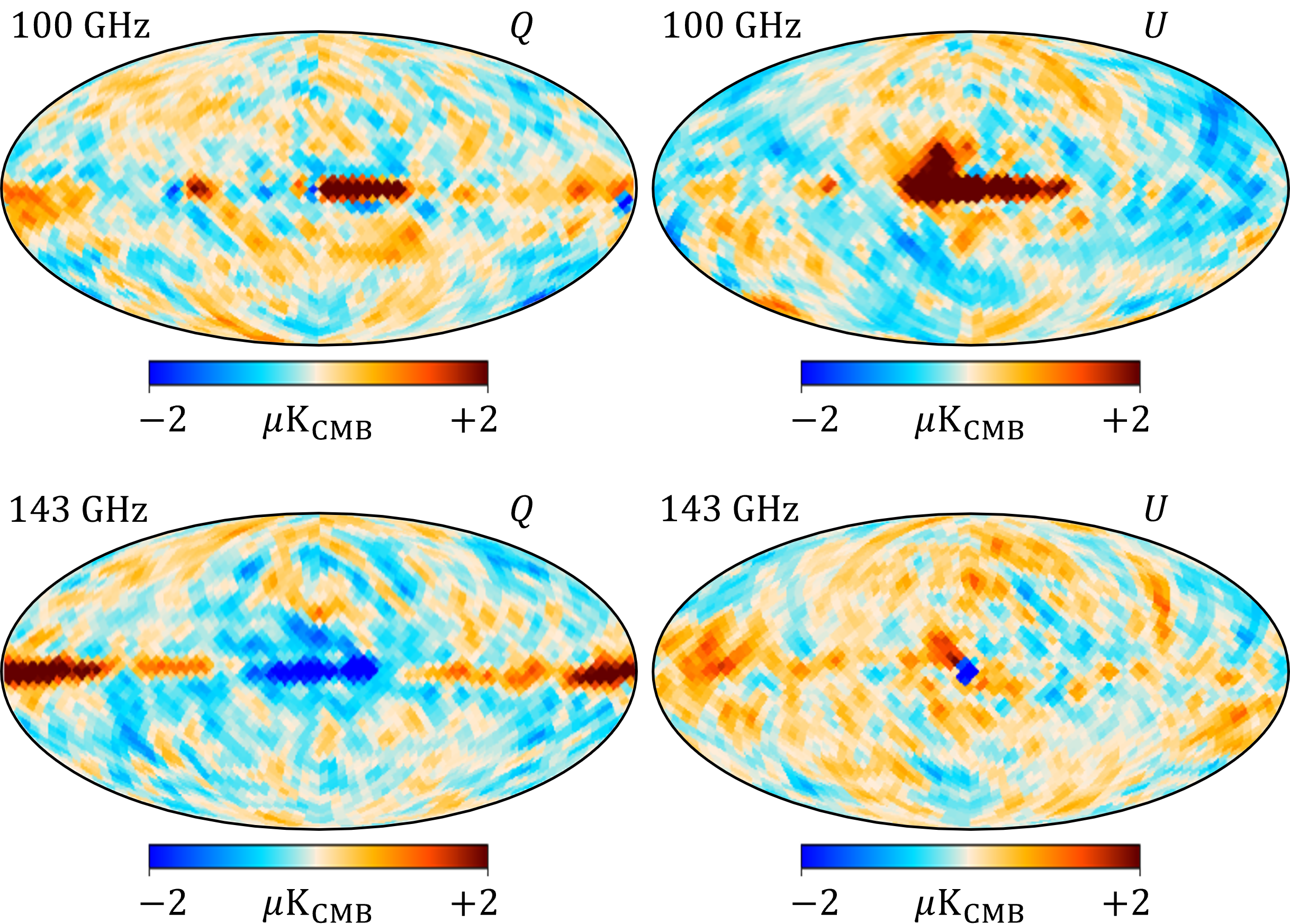
Figure 1: SRoll2 data products of the Planck $Q$ and $U$ maps at frequencies $100$ GHz and $143$ GHz, post component separation, used in this work, displayed in Galactic coordinates.

2.5 Masks

At low Galactic latitudes, the Milky Way emits polarized foreground radiation which dominates the CMB signal in intensity and polarization. Even after component separation, residuals of this emission needs to be excluded from the analysis to avoid biasing cosmological analyses. We therefore apply masks to all maps described in the previous subsections. We consider two of the binary polarization masks published in Pagano et al. (2020), retaining sky fractions of $f_{\rm sky}=\{50\%,60\%\}$. We smooth them with Gaussian beams of corresponding FWHM of $\{15^{\circ},16^{\circ}\}$, and apply a binary threshold, setting all pixels with a value larger than 0.5 to one and all others to zero. This procedure allows us to avoid fuzzy borders and mitigate groups of isolated masked pixels. The smoothed masks are shown in Figure 2. Our baseline mask in this paper is the $f_{\rm sky}=0.5$ smoothed mask, as it retains enough large-scale information to constrain $\tau$, but avoids excessive levels of foregrounds in the Galactic plane.

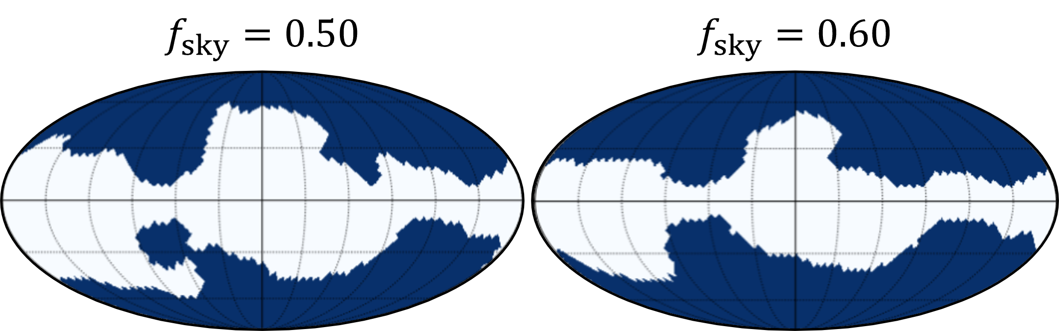
Figure 2: Smoothed version of the SRoll2 sky masks at sky fractions $50\%$ and $60\%$ used in this paper, displayed in Galactic coordinates.

3 NN inference

In this work, we use CNNs to build simulation-based empirical models to perform cosmological inference. In the following, we describe our CNN implementation and give details on the procedures applied to train and test our model on simulations.

3.1 CNN architecture for $\tau$ estimation

CNNs are the industry standard of pattern recognition in 2-dimensional images, performing both classification (e.g., identifying families of objects) and regression tasks (e.g., estimating continuous parameters on maps). The success of CNNs in extracting low-dimensional information from visual input is due to a multi-layer image filtering algorithm. This typically involves searching for distinct sets of local features in the original image (through convolution) and compressing the data (through so-called pooling layers), going to lower and lower resolution, before inferring the desired summary statistic.

In our case, we want to retrieve information from data projected on the sphere, requiring convolutions on the spherical domain. To this end, we make use of the NNhealpix algorithm which allows to build deep spherical CNNs taking advantage of the HEALPix tessellation. In particular, NNhealpix performs convolution by looking at the first neighbors for each pixel on the map, and average pooling by downgrading the map resolution (i.e. by going to lower ${N_{\rm side}}$ parameter). We refer to Krachmalnicoff & Tomasi (2019) for additional details on how the algorithm works, as well as its advantages and disadvantages. In this work, we use NNhealpix in combination with the public keras python package to build our deep CNN architecture, and to perform training, validation and testing.

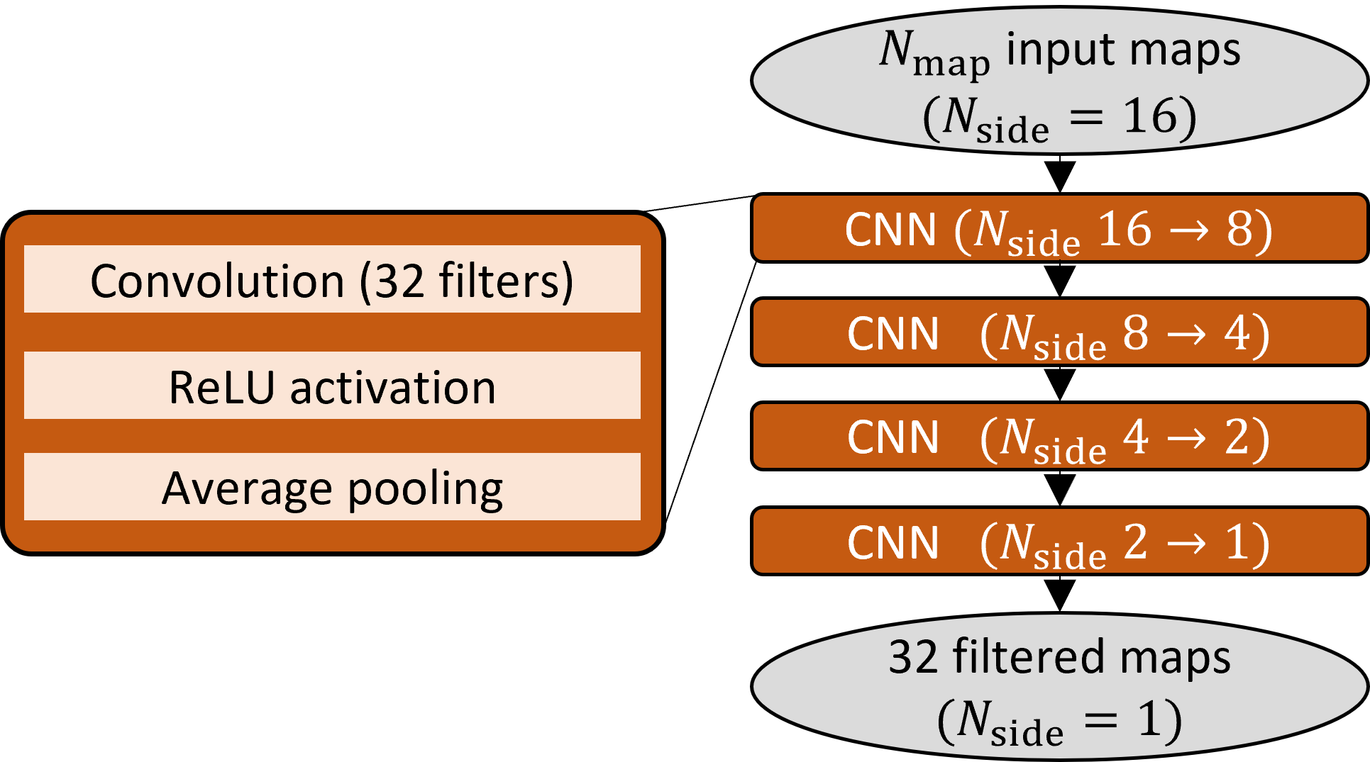
Figure 3: Schematic of the convolutional layers of the neural network used in this paper. This represents the first part of the architecture, performing image filtering.

The first part of our CNN, performing image filtering, consists of four CNN building blocks, as illustrated in Figure 3. We accept $N_{\rm map}$ input maps, which in our case represent one or two frequency channels and Stokes $Q$ and $U$ maps, hence $N_{\rm map}=2$ or 4. Each convolutional layer introduces 32 filters with 9 trainable pixel weights, respectively, and is followed by a Rectified Linear Unit (ReLU) activation layer. Mathematically, this means each image pixel $p_{i}$ undergoes a linear transformation $f$ followed by a nonlinear transformation $g$

$$p_{i}\mapsto p_{i}^{\prime}=(f\circ g)(p_{i})\,,$$ (2)

$$f(p_{i})=p_{i}w_{0}+\sum_{j=1}^{N_{\rm neigh}(i)}p_{k_{j}(i)}w_{j}\,,$$ (3)

$$g(x)\equiv\max(0,x)\;,$$ (4)

where $k_{j}(i)$, $j=1,\dots,\,N_{\rm neigh}(i)$ runs over the indices of all neighboring pixels in the HEALPix map (which can be either 7 or 8, depending on the pixel location). Then, an “average pooling” degradation layer reduces the map resolution from ${N_{\rm side}}$ to ${N_{\rm side}}/2$, assigning to every low-resolution pixel the average of its four children at the next higher resolution. Up to this point, the application of the four CNN building blocks transform the array of input maps at ${N_{\rm side}}=16$ (or $N_{\rm pix}=3072$ pixels) into an array of 32 filtered maps at ${N_{\rm side}}=1$ (or $N_{\rm pix}=12$ pixels). This represents the image filtering part, i.e., the transformation of the original inputs into 32 maximally compressed feature maps that, ideally, retain all the desired (cosmological) information. We still need to “learn” the mapping from theses feature maps to the output numbers $\tau_{\rm NN}$ and $\sigma_{\rm NN}(\tau)$ described in the following section. Compression is done by two fully connected (or dense) layers.

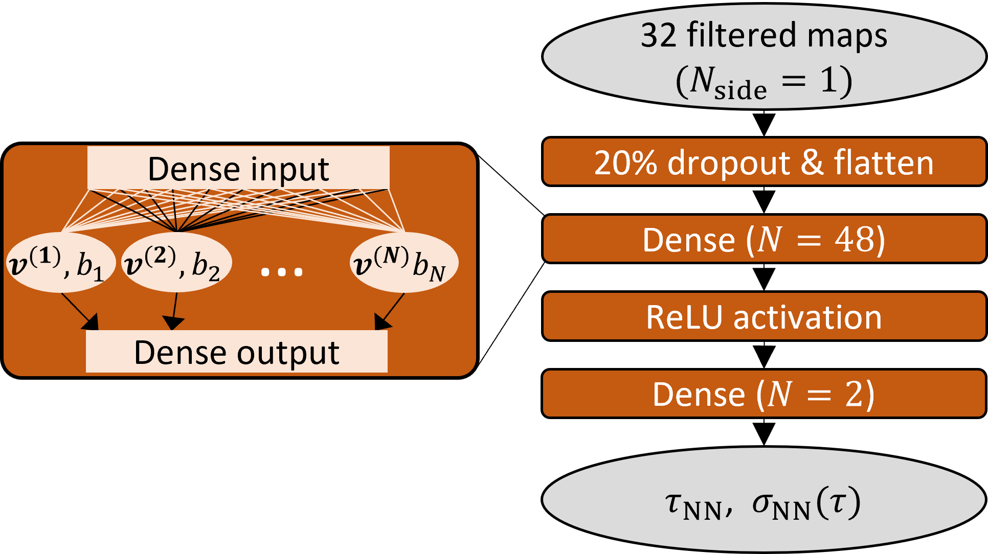
Figure 4: Schematic of the fully connected layers of the neural network used in this paper. This represents the second part of the architecture, performing data compression.

A fully connected layer is a linear map from $M$-dimensional input feature space to $N$-dimensional output feature space, and is commonly used for data compression (in which case $N<M$). A fully connected layer of output dimension $N$ is said to contain $N$ neurons associated to a vector of trainable weights that parameterize the layer. In each of its $N$ neurons, a fully connected layer linearly contracts the input vector $x$ of length $M$ to a number by means of a weights vector $v^{(i)}$,

$$x_{i}\mapsto x^{\prime}_{i^{\prime}}=\sum_{j=1}^{M}v_{j}^{(i^{\prime})}x_{j}\;.$$ (5)

The second part of our CNN, the data compression block, is shown in Figure 4 and contains a dropout and flattening layer, a fully connected layer with 48 neurons, a ReLU nonlinear activation layer, concluded by a final fully connected layer with 2 neurons that outputs $\tau_{\rm NN}$ and $\sigma_{\rm NN}(\tau)$ as described in the following section. The dropout layer acts as a selective off switch for parts of the following fully connected layer, deactivating at random 20$\%$ of its 48 neurons at a time, thus mitigating the overfitting problem common for neural networks (Srivastava et al., 2014). With the described architecture the total number of weights that need to be optimized during training is $N_{\rm w}\approx 4.7\times 10^{4}$.

3.2 Training

When we train a neural network, we effectively tune its many free parameters until the task at hand, e.g. estimating parameters from maps, would be optimally performed on the training data. In the following, we describe this procedure in detail.

At each training step we pass one batch of $N_{\rm batch}=32$ training simulations through the network, meaning we simultaneously consider the results from all simulations that belong to a single batch. Input maps need to be masked with the same mask that is used in the analysis. The output values of the two neurons of the final layer, representing the estimated parameters $\tau_{{\rm NN}j}$, $\sigma_{\rm NN}(\tau)_{j}$ ($j=1,\,\dots,\,N_{\rm batch}$), as well as the truth values $\tau_{j}$, are then inserted into the loss function (Jeffrey & Wandelt, 2020)

$$\mathcal{L}\left[\tau,\;\left(\tau_{{\rm NN}j},\,\sigma_{\rm NN}(\tau)_{j}\right)\right]=$$

$$\sum_{j=1}^{N_{\rm batch}}\left[(\tau_{j}-\tau_{{\rm NN}j})^{2}+\left((\tau_{j}-\tau_{{\rm NN}j})^{2}-\sigma_{\rm NN}(\tau)_{j}^{2}\right)^{2}\right]\;.$$ (6)

We then update all $N_{\rm w}$ network parameters subject to minimizing this loss function. For doing so, we use the Adam optimizer, a widely used stochastic gradient descent algorithm implemented in keras, for which we find an initial training rate of ${\sc LR}=10^{-3}$ and first- and second-moment exponential decay rates $\beta_{1}=0.9$ and $\beta_{2}=0.999$ to be appropriate. Repeating the described procedure for the entire training set of size $N_{\rm train}=190,000$ makes up one training epoch. We train on a maximum of 45 epochs, using the keras callback function ReduceLROnPlateau to allow for learning rates to decrease by a factor of 0.1 if the loss of the validation set has not improved over the course of 5 epochs. Moreover, the callback function EarlyStopping allows for training to stop after a minimum of 20 epochs without improvement in the validation loss. Using both of these callback functions allows a faster convergence and suppresses unwanted oscillations in the loss function during the training phase. Training on a 32-core Intel Xeon CPU node takes about 3 hours, while training on 8 NVIDIA Tesla V100 GPU cores takes about 30 minutes.

3.3 Testing

After training, the neural network parameters are fixed and the model building is in principle completed. However, trained NNs may not perform well for two main reasons: firstly, the loss function may have not converged to its global minimum, causing model predictions to be biased. Secondly, the model may overfit the input, meaning that the network learns the training set’s features with an excellent accuracy, but fails to make correct predictions on similar, independent test sets. Both problems are addressed by testing the model’s predictions on simulations that have not been fed into the network before. We use 2$\times$3 test sets of 10,000 sky simulations with fixed input $\tau=\{0.05$, 0.06, 0.07$\}$, described in detail in Sections 2.2 and 2.3.

4 Results on simulations

Before arriving at the estimation of $\tau$ from the Planck SRoll2 data, we considered several setups to train our CNN model, increasing the complexity of the training simulations. This allowed us to get valuable insight into the learning process. In particular, we start by training the CNN on a set of simulations including CMB+Gaussian noise (see Section 2.2), either on a single frequency channel, or on two channels. We then move to simulations including non-Gaussian systematic effects (i.e. SRoll2 simulations), trying different possible strategies to obtain unbiased $\tau$ estimates in the presence of complex residuals. Only once we achieve this, we apply our trained model to real Planck data. In all the cases presented in this Section, the CNNs are trained and tested considering the $f_{\rm sky}=0.5$ mask as our reference (see Figure 2). A summary of all the analysis cases, along with their corresponding results tables and figures, can be found in Table 1.

Table 1: References to results tables and figures in this paper.

	Gaussian test simulations	SRoll2 test simulations	Planck data
Gaussian NN (1 channel)	Table 2; Figure 5	Table 3; Figure 5
Gaussian NN (2 channels)	Table 2; Figures 5, 8	Table 3; Figures 5, 8	Table 5; Figures 9, 10
HL likelihood	Table 2	Table 3
SRoll2 training		Table 4
SRoll2 retraining		Table 4; Figure 8	Table 5; Figures 9, 10
Empirical likelihood			Table 5; Figure 10

4.1 Gaussian training

As aforementioned, we first test the ability of our CNN to estimate the value of $\tau$ considering only Gaussian noise. These simulations have noise amplitudes and pixel-pixel correlations directly estimated from Planck maps, and therefore serve as a good description of the Gaussian noise present in real data. At the same time they lack for realism, since they do not include non-Gaussian residual systematic effects, contamination due to Galactic foregrounds, both known to be present on the Planck SRoll2 maps. We therefore expect these models (which we refer to as “Gaussian models”) to induce a bias on $\tau$ when applied to the more realistic SRoll2 simulations, or to real Planck data.

4.1.1 Single channel

We begin by training our CNN on Stokes $Q$ and $U$ maps with Gaussian Planck-like noise and CMB at $143$ GHz only, thus feeding $N_{\rm map}=2$ maps to the network. In the left hand side of Table 2, we show the results of testing $N_{\rm sims}=10,000$ Gaussian simulations of CMB and noise generated with fiducial $\tau=0.05$, $0.06$ and $0.07$, respectively. The average learnt mean posterior values $\overline{\tau_{\rm NN}}$ are close to unbiased and deviate at the 0.2$\sigma$ level. The average learnt posterior standard deviations $\overline{\sigma_{\rm NN}(\tau)}$ are within $5\%$ agreement with the sample scatter across simulations, $\sigma(\tau_{\rm NN})$.

To assess the performance of the Gaussian model also on non-Gaussian Planck-like maps, we tested this model on 10,000 SRoll2 simulations generated with fiducial $\tau=0.06$ (see Section 2.3). As illustrated in the upper right panel of Figure 5, this leads to a $>1\sigma$-bias on $\tau_{\rm NN}$. These tests on a single frequency channel leave us with two conclusions: on the one hand, CNNs are able to correctly retrieve $\tau$ and its statistical uncertainty from a single Planck-like simulation of the 143 GHz channel containing correlated Gaussian noise. On the other hand, systematic effects present in the Planck SRoll2 simulations bias the single-channel CNN inference, as expected. To improve our results, we add another frequency channel to the inference pipeline, seeking to mitigate this bias. We expect that combining two channels should lead to a lower error bar and a lower bias on the SRoll2 simulations, in a similar way as cross-spectra achieve lower noise bias than auto-spectra.

4.1.2 Two channels

As a second test, we add the HFI channel at 100 GHz in the training and testing procedures, simulated as CMB plus the corresponding Gaussian correlated noise, so that $N_{\rm map}=4$ maps are fed into the neural network. The results from testing on Gaussian noise are shown in Table 2. We note two positive effects: firstly, the small bias observed for Gaussian noise on a single channel is further reduced to below $1\%$ of a standard deviation. Secondly, the learnt $\sigma_{\rm NN}(\tau)$ decreases by more than $10\%$ when training on two frequency channels. Meanwhile, the prediction of the posterior standard deviation stays within $5\%$ of the sample standard deviation of the inferred $\tau_{\rm NN}$. The same results are visualized in Figure 5 for fiducial $\tau=0.06$, showing significant improvement of the two-channel CNN inference in the lower panels with respect to the one-channel results (upper panels). We proceed to test this two-channel Gaussian model on the SRoll2 simulations. As shown in the right panel of Figure 5, for fiducial $\tau=0.06$, the addition of a second channel allows for a significant reduction of the systematic-related bias in $\tau_{\rm NN}$ and to a better statistical constraint. This leads us to conclude that CNNs are able to recognize common features across channels, combining the information to reduce the statistical uncertainty and to efficiently ignore uncorrelated systematic effects.

The corresponding quantitative results, for all the three $\tau$ values used during testing, are found in Table 3: adding a second channel in the Gaussian training model leads to improved results on the SRoll2 test simulations for all considered values of $\tau$. However, a residual bias is still present, especially when the CMB signal is smallest, i.e. for $\tau=0.05$.

Moreover, we notice that, when applied to the SRoll2 test maps, the models trained on Gaussian simulations return values of $\sigma_{\rm NN}(\tau)$ not in agreement with the actual spread of estimates $\sigma(\tau_{\rm NN}$), with the latter being up to $\sim 25\%$ larger. This implies that the learnt error is not accurate in this case, and therefore cannot be used to described the uncertainties of our inferred $\tau$ values on SRoll2 maps. We will address error bars in Section 4.4.

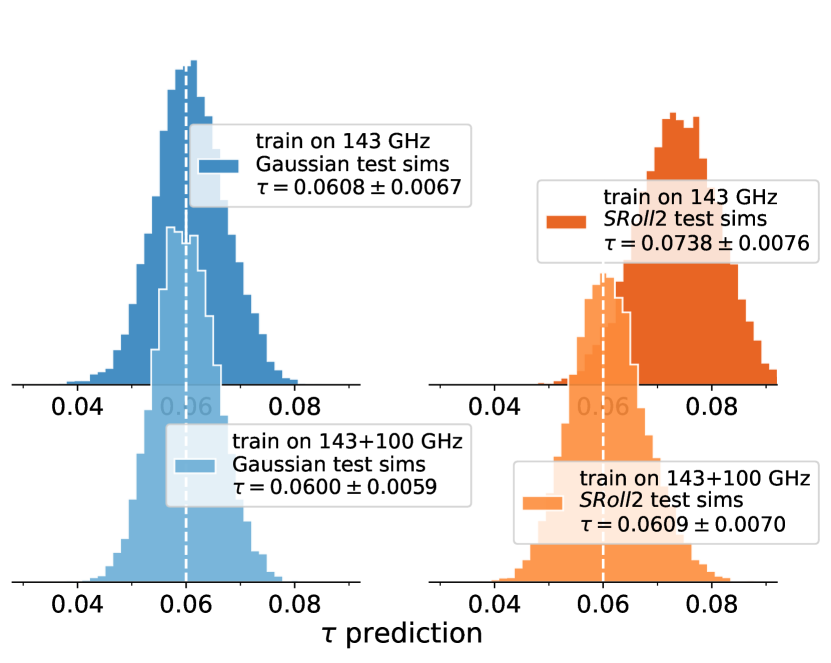
Figure 5: Predictions of $\tau_{\rm NN}$ from $10,000$ simulations with input $\tau=0.06$, containing either CMB with Gaussian noise (left panels) or CMB with SRoll2 noise + systematics (right panels). The two rows denote different CNN models trained on CMB with Gaussian noise on a single frequency channel (top), on two frequency channels (bottom).

Table 2: $\tau$ predictions from $10,000$ Gaussian CMB + noise simulations generated with three different, fixed fiducial $\tau$ values. We show Gaussian training results on one and two channels, respectively, as well as power spectrum likelihood results. Shown are the posterior mean $\tau_{\rm NN/HL}$ and standard deviation $\sigma_{\rm NN/HL}(\tau)$ averaged over all simulations, as well as the scatter of $\tau_{\rm NN/HL}$ over all simulations.

Test on Gaussian simulations
	143 GHz			143+100 GHz			143$\times$100 GHz
	Gaussian training			Gaussian training			HL likelihood
fiducial $\tau$	$\overline{\tau_{\rm NN}}$	$\overline{\sigma_{\rm NN}(\tau)}$	$\sigma(\tau_{\rm NN})$	$\overline{\tau_{\rm NN}}$	$\overline{\sigma_{\rm NN}(\tau)}$	$\sigma(\tau_{\rm NN})$	$\overline{\tau_{\rm HL}}$	$\overline{\sigma_{\rm HL}(\tau)}$	$\sigma(\tau_{\rm HL})$
0.05	0.0508	0.0059	0.0066	0.0503	0.0054	0.0057	0.0496	0.0046	0.0047
0.06	0.0608	0.0065	0.0067	0.0600	0.0056	0.0059	0.0596	0.0048	0.0048
0.07	0.0712	0.0067	0.0070	0.0702	0.0057	0.0063	0.0697	0.0048	0.0049

Table 3: Same as Table 2, but testing on CMB and SRoll2 simulations instead of CMB and Gaussian noise simulations.

Test on SRoll2 simulations
	143 GHz			143+100 GHz			143$\times$100 GHz
	Gaussian training			Gaussian training			HL likelihood
fiducial $\tau$	$\overline{\tau_{\rm NN}}$	$\overline{\sigma_{\rm NN}(\tau)}$	$\sigma(\tau_{\rm NN})$	$\overline{\tau_{\rm NN}}$	$\overline{\sigma_{\rm NN}(\tau)}$	$\sigma(\tau_{\rm NN})$	$\overline{\tau_{\rm HL}}$	$\overline{\sigma_{\rm HL}(\tau)}$	$\sigma(\tau_{\rm HL})$
0.05	0.0669	0.0065	0.0074	0.0536	0.0055	0.0067	0.0478	0.0050	0.0079
0.06	0.0738	0.0067	0.0076	0.0609	0.0056	0.0070	0.0585	0.0050	0.0073
0.07	0.0813	0.0069	0.0074	0.0690	0.0057	0.0071	0.0688	0.0049	0.0069

4.2 Comparison with Bayesian inference from cross-QML power spectrum estimates

In this section we compare NN inference results with results coming from a standard Bayesian approach applied to $E$-mode power spectra. In particular, we consider quadratic Maximum Likelihood (QML) estimates (e.g. Tegmark & de Oliveira-Costa (2001)) of the 100$\times$143 GHz $EE$ cross-spectrum, and take posterior samples using the well-known power spectrum likelihood approximation introduced by Hamimeche & Lewis (2008) (in the following HL likelihood). The HL likelihood provides a good approximation to the non-Gaussian distribution of the exact power spectrum likelihood, which markedly differs from Gaussianity at low multipoles $2\leq\ell\lesssim 30$ most relevant for constraining $\tau$. Evaluating the HL likelihood requires a power spectrum covariance matrix, which we obtain directly from simulations of Gaussian noise and CMB realized with the same $\tau$ values used for generating the test simulations (Section 2). For the HL likelihood we assume a theoretical model of the CMB $E$-modes, computed with CAMB, considering the multipole range $2\leq\ell\leq 30$, and sampling only for the $\tau$ parameter, keeping $10^{9}A_{s}e^{-2\tau}=1.884$ fixed. Our final results are the best-fit value $\tau_{\rm HL}$, the standard deviation $\sigma_{\rm HL}(\tau)$ of the posterior, and the scatter $\sigma(\tau_{\rm HL})$ computed from the set of test simulations.

We run the HL likelihood on $3\times 10,000$ Gaussian sky simulations with input $\tau=0.05,\,0.06$ and 0.07. As shown in the last three columns of Table 2, we find unbiased best-fit results with average posterior standard deviation $\overline{\sigma_{\rm HL}(\tau)}$ and best-fit parameter scatter $\sigma(\tau_{\rm HL})$ of $\sim 0.0048$. We notice that the uncertainties derived from sampling the HL likelihood are $\sim 20\%$ smaller than the ones from NN estimates. Part of the scatter of $\tau_{\rm NN}$ comes from the intrinsic stochastic nature of the training process, and could be reduced by taking the average over multiple NN models (as discussed in Section 4.4). Nevertheless, these results reveal that although we are able to retrieve unbiased $\tau$ values with NNs from Gaussian simulations, our estimator does not achieve minimum variance. Further development of the method, including an optimization of the convolution algorithm on the sphere, the NN architecture and the training procedure, are required and will be explored in the light of improving the estimator’s variance.

In addition to Gaussian simulations, we apply the cross-spectrum inference pipeline on $3\times 10,000$ SRoll2 simulations and show the corresponding results in the last three columns of Table 3. We stress that the HL likelihood contains the same covariance matrix as before, calculated from Gaussian simulations. This is done in analogy with the case of Gaussian NN training applied to SRoll2 simulations, therefore neglecting the presence of systematic effects. We retrieve biased estimates on $\tau$, confirming our expectation that the power spectrum model implemented in the likelihood is an inaccurate representation of the SRoll2 simulations, which include spurious non-Gaussian signals. Interestingly, this affects the NN and HL estimates in different ways, leading to biases in opposite directions for $\tau=0.05$ and $0.06$. To study the relative behavior of the two estimators, it is instructive to look at a one-by-one comparison of the NN and HL results on the same 10,000 test simulations, as presented in Figure 6 for $\tau=0.06$. The scatter plot of the estimated $\tau_{\rm NN}$ and $\tau_{\rm HL}$ on Gaussian simulations and on SRoll2 simulations are shown in bright red and dark green, respectively. In the Gaussian case the correlation of the estimated $\tau$ values is at a level of $\sim 76\%$, while for SRoll2 it is at $63\%$. Therefore systematic effects, present on the maps and partially unaccounted for in the estimates, decrease the correlation and increase the differences between $\tau_{\rm HL}$ and $\tau_{\rm NN}$ when going from Gaussian to SRoll2 test simulations, indicating that the two estimators are impacted differently by spurious non-Gaussian signals.

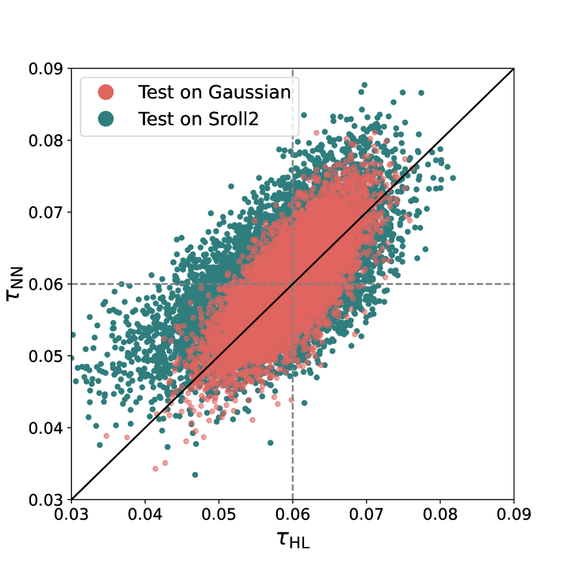
Figure 6: Per-simulation comparison between the HL likelihood estimate $\tau$ and the NN estimate $\tau_{\rm NN}$ for a test set of 10,000 simulations realized with $\tau=0.06$. Gaussian simulations are shown in bright red, SRoll2 simulations in dark green. The correlation coefficient between both estimators are $76\%$ (Gaussian) and $63\%$ (SRoll2).

.

4.3 Training including systematic effects

As previously seen, the two-channel Gaussian training allows to improve our $\tau$ estimates on SRoll2 simulations. However, the persistence of residual bias motivates us to move forward in the training setup and include systematic effects in the training simulations. Our goal is to achieve fully unbiased results as a necessary condition to apply our NN models to real Planck maps. In this section we explore two possible ways of including systematics in our NN-based models: training on SRoll2 simulations from the very beginning, and performing a SRoll2 retraining update on previously trained Gaussian networks.

4.3.1 Training on SRoll2 simulations

Table 4: $\tau$ predictions from $10,000$ CMB + SRoll2 test simulations generated with three different fiducial $\tau$ values. We show results using two frequency channels, either training on SRoll2 from the start, or retraining on SRoll2 maps. Displayed are the average posterior mean, average predicted standard deviation $\overline{\sigma_{\rm NN}(\tau)}$ and the scatter $\sigma(\tau_{\rm NN})$ calculated across the test simulations.

Test on SRoll2 simulations
	143+100 GHz			143+100 GHz
	SRoll2 training			SRoll2 retraining
fiducial $\tau$	$\overline{\tau_{\rm NN}}$	$\overline{\sigma_{\rm NN}(\tau)}$	$\sigma(\tau_{\rm NN})$	$\overline{\tau_{\rm NN}}$	$\overline{\sigma_{\rm NN}(\tau)}$	$\sigma(\tau_{\rm NN})$
0.05	0.0526	0.0059	0.0066	0.0508	0.0077	0.0091
0.06	0.0622	0.0062	0.0070	0.0606	0.0079	0.0088
0.07	0.0722	0.0064	0.0070	0.0707	0.0081	0.0087

The SRoll2 simulations (Delouis et al., 2019) are designed to accurately describe Planck’s Gaussian noise component and non-Gaussian polarization systematics. Motivated by this, we train a CNN from the start on the 200,000 SRoll2 training simulations described in Section 2.3. As usual, we use 190,000 simulations to perform weight optimization, and 10,000 for validation. We train on Planck’s 143 GHz and 100 GHz channels simultaneously and use the same hyper-parameter values as for the Gaussian training, described in Section 3.2. We stress that even though artificially augmented by forming new channel pair combinations, the SRoll2 training set is essentially built from $400$ sampled skies only. The testing is performed on $3\times 10,000$ SRoll2 simulations with fixed $\tau=0.05$, 0.06 and 0.07, generated from the remaining 100 independent realizations that were not seen by the CNN during training.

Results obtained with this approach are displayed in Table 4. For the three input $\tau$ values we find a positive bias of $\sim 0.4\sigma$. For $\tau=0.06$, the average learnt error $\overline{\sigma_{\rm NN}(\tau)}=0.0062$, slightly larger than for the two-channel Gaussian training but smaller than the scatter $\sigma(\tau_{\rm NN})=0.0070$ similar to what we see both for the Gaussian CNN and the HL likelihood inference (see Table 3). As in the case of Gaussian NN training, the learnt error does not agree with the SRoll2 simulation scatter, therefore it cannot be used to infer the statistical uncertainty on $\tau_{\rm NN}$.

We ascribe the main reason for the bias on $\tau$ to overfitting. Figure 7 illustrates the problem: we compare the $\tau$ predictions on a set of 10,000 test simulations with the ones coming from 10,000 training simulations. The results show a bias and standard deviation of $\Delta\tau=0.0023\pm 0.0069$ for the test set, while the training set is unbiased, with $\Delta\tau=0.0001\pm 0.0068$. This is clear evidence for overfitting: while the model performs well on the 400 SRoll2 simulations that the training set is built from, these are not enough to generalize to the remaining 100 SRoll2 simulations used to build the test set, leading to the observed bias on $\tau$ in the latter case.

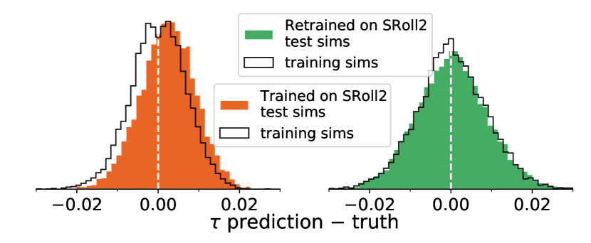
Figure 7: Neural network accuracy in predicting the true $\tau$ input from $10,000$ simulations. Step-filled histograms show the results on unseen test simulations, black outlines show the results on a subset of the actual training simulations. We compare a network exclusively trained on SRoll2 simulations (left panel) with a Gaussian network retrained on SRoll2 simulations (right panel).

4.3.2 Retraining update with SRoll2 simulations

We recognize the bias described above as a critical problem that needs to be addressed. The obvious option, training on a considerably higher number of simulations, is unavailable due to the limited number of published SRoll2 realizations. Therefore, we apply a transfer learning technique to inform our previously trained Gaussian networks about SRoll2 systematics. In the previous sections we demonstrated that our Gaussian CNN model is not affected by overfitting issues and, if trained on two channels, performs reasonably well even on SRoll2 simulations. This motivates us to leverage the existing results on Gaussian networks to solve the overfitting issue with as little changes as possible. To this end, we choose the approach of retraining the two-channel Gaussian model on the full set of SRoll2 training simulations, while targeting two specific goals:

• The retrained CNN should learn to extract information on the systematic effects present in the SRoll2 simulations, and update its CNN weights just enough to achieve fully unbiased results on the SRoll2 training set.

• At the same time, we want to ensure that the information already learnt is not destroyed during the new training phase (an issue sometimes referred to as catastrophic forgetting, see e.g. Kirkpatrick et al. (2017), Ramasesh et al. (2021)), avoiding going back to the overfitting situation described in the previous section.

We achieve this by performing what we call “minimal retraining”: we choose the hyper-parameters of the NN such that we obtain unbiased results on the SRoll2 test simulations while making minimal changes to the original network. We find an optimal setup by setting the number of retraining epochs to 5 while choosing a small learning rate of $LR=10^{-7}$, without making any additional changes to the original network architecture.

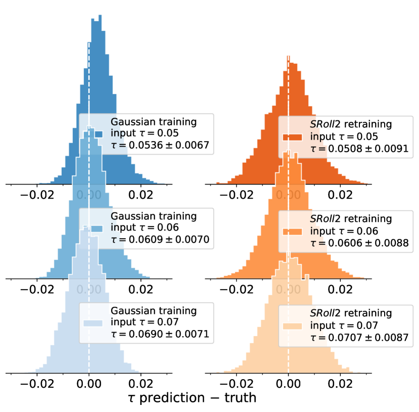
Figure 8: Predictions of $\tau_{\rm NN}$ on $10,000$ SRoll2 simulations with input $\tau=0.05$, 0.06 and 0.07 (first, second, third row, respectively). The two columns display two different NN models trained on two channels of Gaussian simulations (left panels), and retrained on two channels of SRoll2 simulations (right panels). All result are for $f_{\rm sky}=0.5$.

The right panel of Figure 7, in complete analogy to the left panel, compares the distribution of $\Delta\tau$ from the SRoll2-retrained model on training simulations (black contours), or test simulations (green filled histogram). We find both histograms in good agreement, indicating that unlike the SRoll2-trained model, the retrained model does not suffer from overfitting, thus achieving our goal (ii) defined above. Table 4 on the right-hand side lists the results of the SRoll2-retrained model on SRoll2 test simulations. We find $\overline{\tau_{\rm NN}}=0.0508$, 0.0606 and 0.0707 for the respective input values of $\tau=0.05$, 0.06 and 0.07. This amounts to a bias below $\Delta\tau=8\times 10^{-4}$, or $\lesssim 0.1\sigma$. In Figure 8 we show a comparison of the results on SRoll2 test sets obtained by Gaussian versus SRoll2-retrained CNNs. The reduction of the bias is evident, in particular for $\tau=0.05$. Therefore, we choose the retrained approach as our baseline model to estimate $\tau$ on real Planck data. At the same time, this approach brings an increase in $\sigma(\tau_{\rm NN})$, an effect not seen with the SRoll2 training procedure described in Section 4.3.1. This could be the consequence of the typical variance-bias trade-off observed between statistical estimators: with minimal retraining we are able to achieve unbiased estimates (goal (i) above) at the cost of a larger $\sigma(\tau_{\rm NN})$. In addition to that, we are still unable to retrieve values of the learnt $\sigma_{\rm NN}(\tau)$ that agree with $\sigma(\tau_{\rm NN})$ for SRoll2 simulations (and therefore also for Planck data). We conclude that, differently from what happens in the Gaussian model tested on Gaussian simulations, we cannot use the learnt error as an estimate of the uncertainty of the inferred $\tau_{\rm NN}$.

4.4 NN errors

The loss function in Equation (6) provides an estimate for the posterior standard deviation $\sigma_{\rm NN}(\tau)$. However, as seen in the previous sections, the learnt $\sigma_{\rm NN}(\tau)$ tends to underestimate the actual spread of the inferred values of $\tau_{\rm NN}$ on test set maps, especially in the case of SRoll2 maps. We therefore proceed to empirically estimate our errors from simulations.

In doing so, we need to make an additional consideration: training a NN is an intrinsically stochastic procedure that relies upon the use of a stochastic optimizer, randomly initialized NN weights and random realizations of the maps in the training set. This results in the fact that each NN prediction can be described as the sum of two random variables: $\tau_{\rm NN}=\tau+\Delta_{\rm NN}$, and therefore

$$\sigma^{2}(\tau_{\rm NN})=\sigma^{2}(\tau)+\sigma^{2}(\Delta_{\rm NN})+2\,{\rm Cov}(\tau,\Delta_{\rm NN})\,,$$ (7)

where the first source of uncertainty, $\sigma(\tau)$, is due to noise and cosmic variance of test simulations or observed data, while the second, $\sigma(\Delta_{\rm NN})$, represents the stochasticity of the NN estimator. These two terms are sometime referred to as aleatory and epistemic error, respectively (Hüllermeier & Waegeman, 2021).

We can measure the uncertainty related to the NN stochasticity by training an ensemble of models, all based on the same architecture and hyper-parameters, but with different initial weights and training set realizations. Our estimate of $\sigma(\Delta_{\rm NN})$ is given by the the standard deviation of the models’ $\tau$ predictions when tested on a single test map. In practice, we define the “model ID” of a trained NN as the fixed random seed controlling the initialization of network weights. We generate a new training set of simulations whose specific realizations (of CMB, noise and potentially systematics) is fully determined by the model ID. Following this recipe, we create 100 independent Gaussian training sets and use them to train 100 Gaussian networks. Repeating this procedure with 100 SRoll2 training sets, we retrain the set of 100 Gaussian networks to obtain 100 SRoll2-retrained networks. Using a single test map with input $\tau=0.06$, we find $\sigma(\Delta_{\rm NN})\simeq 0.0024$ for Gaussian NN models tested on Gaussian maps, and $\sigma(\Delta_{\rm NN})\simeq 0.0034$ for minimally retrained NN models tested on SRoll2. In both cases this represents about $40\%$ of the corresponding value of $\sigma(\tau_{\rm NN})$ reported in Tables 2 and 4, respectively.

We can reduce the impact of the NN stochasticity by taking, for each test map, the ensemble average of the $\tau$ estimates over the 100 trained NNs. By doing so, for the case with $f_{\rm sky}=0.5$ and input $\tau=0.06$, we find $\sigma(\tau_{\rm NN})\simeq 0.0054$ for Gaussian models applied to Gaussian maps and $\sigma(\tau_{\rm NN})\simeq 0.0083$ for retrained models applied to SRoll2 simulations.

We also evaluate the correlation coefficient between the predictions of pairs of models $(j,k)$, tested on the same 10,000 simulations, for both Gaussian and SRoll2 training and testing, respectively. In both cases, we find $\rho_{jk}\simeq 0.84$, in agreement with what is expected if Equation (7) holds and the models’ epistemic errors are uncorrelated, ${\rm Cov}(\Delta^{j}_{\rm NN},\Delta^{k}_{\rm NN})=\delta^{\mathcal{K}}_{jk}\sigma^{2}(\Delta_{\rm NN})$. In the following section we apply our CNN models to Planck maps to infer the value of $\tau$ from data, estimating its uncertainty from simulations and using the ensemble average over 100 trained models to reduce the impact of the NN stochasticity.

5 Results on Planck data

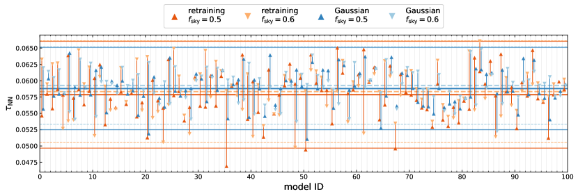
Figure 9: NN predictions of $\tau$ from Planck 100+143 GHz data, resulting from training 100 equivalent models with different random initial weights and random seeds for training data, considering Gaussian two-channel training (blue tones) versus SRoll2 retraining (orange tones), and $f_{\rm sky}=0.5$ (downward triangles) versus $f_{\rm sky}=0.6$ (upward triangles). Colored triangle markers show the best-fit values for the single models and horizontal lines in the corresponding colors show the ensemble average of $\tau$ (middle) $\pm$ the $68\%$ confidence interval (upper and lower lines).

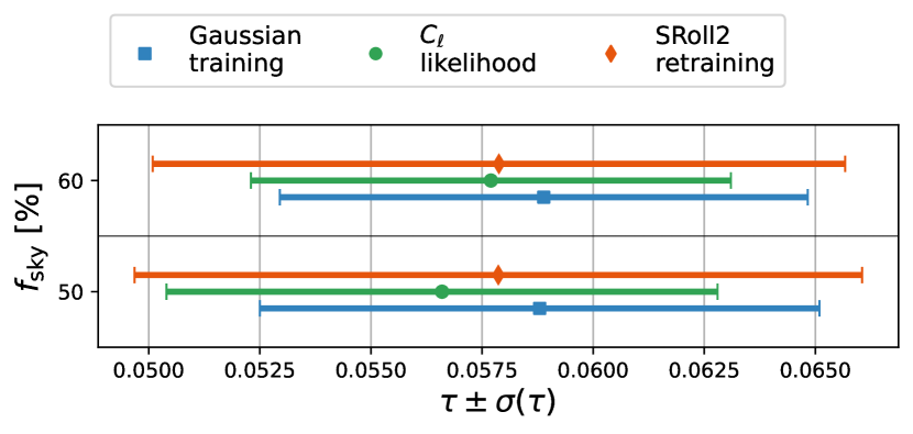
Figure 10: Results on $\tau$ obtained from Planck SRoll2 data. The values in this plot are shown in Table 5.

Table 5: Results from Planck data on two different sky masks, using Gaussian NNs, SRoll2-retrained NN models and the empirical $C_{\ell}$-based likelihood presented in Pagano et al. (2020). The NN results are averaged over 100 models, and $\sigma(\tau_{\rm NN})$ is computed from 10,000 simulations with input $\tau=0.058$.

Predictions on Planck SRoll2 data
	143+100 GHz		143+100 GHz		143x100 GHz
	Gaussian training		SRoll2 retraining		$C_{\ell}$ likelihood
$f_{\rm sky}$	$\tau_{\rm NN}$	$\sigma(\tau_{\rm NN})$	$\tau_{\rm NN}$	$\sigma(\tau_{\rm NN})$	$\tau$	$\sigma(\tau)$
$50\%$	0.0588	0.0063	0.0579	0.0082	0.0566	0.0062
$60\%$	0.0593	0.0059	0.0583	0.0078	0.0577	0.0054

As shown in Sections 4.3.2 and 4.4, by retraining on the SRoll2 simulations, we are able to obtain a CNN-based model that yields unbiased results on unseen SRoll2 test simulations generated with fixed $\tau\in\{0.05,\,0.06,\,0.07\}$. Having thus confirmed the robustness of our method, we now move to real Planck data and proceed to predict $\tau$ from the 100 and 143 GHz SRoll2 HFI maps.

Our baseline $\tau$ estimate is obtained by taking the average of the inferred values from the 100 minimally retrained NNs applied to Planck data for a sky mask with $f_{\rm sky}=0.5$, resulting in a mean estimate of $\tau_{\rm NN}\simeq 0.0058$. Figure 9 shows the obtained $\tau$ values for each of these NN models. Following the conclusions of the previous sections, since the learnt $\sigma_{\rm NN}(\tau)$ is inadequate as an error prediction, we estimate the uncertainty from simulations. In practice, we generate a set of 10,000 SRoll2 simulations realized with $\tau=0.058$ and average the $\tau_{\rm NN}$ estimates over 100 networks. Afterwards, we compute the standard deviation over 10,000 simulations. Our final inference on Planck maps in this baseline case results in:

$$\tau_{\rm NN}=0.0579\pm 0.0082\quad({\it Planck}{}\,{\rm 100}+{\rm 143\,GHz})\,.$$ (8)

This value is in very good agreement with the $\tau$ estimates obtained with an empirical likelihood based on cross-QML power spectra, presented in Pagano et al. (2020) (hereafter P2020) applied to the same Planck maps and constructed from the same SRoll2 simulations that we use in this work. In particular, P2020 obtained $\tau=0.0566\pm 0.0062$ on the $f_{\rm sky}=0.5$ sky mask. We notice that the uncertainty from our NN method is $\sim 30\%$ larger. As previously described, this is due to the fact that our NN estimator does not reach minimum variance and that we rely on the retraining strategy that leads to larger errors. However, the fact that we obtain a $\tau$ value in agreement with the one reported in the literature, considering that we are using an inherently different inference approach based, for the first time, on NNs, represents a remarkable result of this work.

We also apply the Gaussian NN model to Planck data, deriving the best-fit parameter value and error bars analogously. Note that, although the Gaussian model leads to results that are mildly biased by up to $\sim 0.5\sigma$ when applied to SRoll2 maps with low CMB input signal ($\tau=0.05$), the bias is below $0.15\sigma$ when $\tau=0.06$, as displayed in the 5th column of Table 3. In this case, using the same $f_{\rm sky}=0.5$ mask, we obtain $\tau_{\rm NN}=0.0588\pm 0.0063$. The statistical uncertainty is lower for this second method, as we omit retraining on systematics, and similar to the one obtained from the empirical likelihood presented in P2020.

Lastly, as a robustness test, we apply the same methods to a second sky mask, with a larger sky coverage of $f_{\rm sky}=0.6$. Results on parameter estimation are stable for both retrained and Gaussian model, while uncertainties are reduced. The NN predictions of the single models on $f_{\rm sky}=0.6$ are displayed in Figure 9. A summary of our results on Planck maps is shown in Figure 10 and Table 5.

6 Conclusions

In this paper, we present the first cosmological parameter inference on Planck’s CMB polarization maps that is performed entirely by neural networks. We estimate the optical depth to reionization, $\tau$, from the SRoll2 low resolution polarization maps of Planck-HFI at 100 and 143 GHz. These maps are known to contain a significant level of residual systematic effects at large angular scales that, if ignored, would bias cosmological results. These spurious signals are non-Gaussian and hard to model in an analytical way. For this reason, in the literature (Pagano et al., 2020, P2020), the estimation of $\tau$ from these maps is obtained by sampling an empirical $EE$ cross-spectrum likelihood (Planck Collaboration V, 2020; Gerbino et al., 2020), built from a set of realistic SRoll2 simulations (Delouis et al., 2019).

In this work, we approach this problem through NN-based inference applied directly on the map domain. One of the benefits of this method is that it does not require an analytical model of the data but, instead, relies solely on using simulations to train a regression model. In particular, we use the NNhealpix algorithm to build our NN models, allowing the application of convolutional layers on the sphere. We consider several setups to train and validate CNNs on multiple sets of simulations, before applying them to Planck data. We adopt the moments loss function of Jeffrey & Wandelt (2020) to learn the mean and standard deviation of the marginal posterior on $\tau$ inferred from Stokes $Q$ and $U$ maps pixelized on a grid at ${N_{\rm side}}=16$ ($\sim 4^{\circ}$). To find the best training method, we start from simulations of a single frequency channel of CMB with coadded Gaussian correlated noise and, step by step, move to more complex setups that involve two frequency channels containing CMB, noise and systematic effects. We compare the results obtained with NNs with the ones from a standard Bayesian method that applies the HL likelihood to $EE$ cross-spectra. Our main results and conclusions from the analysis applied to simulations are the following:

1. When trained and applied to Gaussian simulations, the NN models are able to retrieve unbiased values of $\tau$ directly from maps. Additionally, by using the moments loss function reported in Equation (6), the models can also learn and return an error estimate that is consistent with the spread of the best-fit values on the test set.

2. When trained using maps from two frequency channels that share the same cosmological signal, the NNs are able to effectively combine the information from both maps. This leads to improved accuracy in the $\tau$ estimates and smaller uncertainties. This ability to combine information from different channels is a key advantage of the NN approach as, in the future, it would allow for a straightforward combination of all available data sets without the need for a joint model, thus reducing the impact of noise and systematics.

3. A comparison of the NN estimates with the ones obtained from the HL cross-spectrum method applied to Gaussian simulations shows that the NN approach leads to higher uncertainties by about 20%. This implies that the NN estimator, although unbiased, does not reach the minimum variance. In order to further improve the performance of the estimator, future work should focus on optimizing the spherical convolution algorithm, the model architecture, and the training procedure. This will help to minimize the uncertainties and reach the best possible performance.

4. The application of the Gaussian two-channel model to the SRoll2 simulations, which include systematic effects, leads to inaccurate estimates on $\tau$, as does the use of the HL likelihood. Although expected, this observed bias is much smaller (nearly unbiased for $\tau\sim 0.06$) than that seen for the single-channel model, demonstrating that the neural network is able to identify common features in the maps, efficiently ignoring the uncorrelated signal between different channels.

5. To recover fully unbiased results on SRoll2 maps, as a prerequisite to apply our NN model to Planck data, we need to train NNs on maps that incorporate instrumental systematic effects. Due to the limited number of available SRoll2 simulations, we adopt a minimal retraining approach, building on the good results already obtained with the Gaussian models. This approach helps to minimize overfitting issues, but it also leads to slightly larger errors in the recovered $\tau$ values.

6. In more complex scenarios, when the NN models are applied to the SRoll2 maps, we find that the error estimate learned by the NN, $\sigma_{\rm NN}(\tau)$, underestimates the spread evaluated on the empirical distribution of the test maps, $\sigma(\tau_{\rm NN})$. This suggests that the NN model is not capturing the full range of uncertainty in the data. To overcome this issue, we proceed by evaluating the final error on $\tau$ through simulations, by taking the ensemble average of 100 NN models. This helps to reduce the impact of the epistemic uncertainty caused by the intrinsic stochasticity of the NN estimator.

After evaluating and validating the performance of the NNs on simulations, we apply our trained models to Planck SRoll2 maps at 100 and 143 GHz. For the minimally retrained model, which is the one that leads to fully unbiased results on the SRoll2 simulations, we obtain $\tau_{\rm NN}=0.0579\pm 0.0082$ on our fiducial $f_{\rm sky}=0.5$ mask. This value is in very good agreement with the one obtained from the empirical likelihood based on cross power spectra reported in P2020, which relies on the same set of simulations. We consider this a remarkable result of our work, given the fact that the two estimators are intrinsically different. However, we note that our final uncertainty on the $\tau_{\rm NN}$ estimate, evaluated through simulations and involving the ensemble average of 100 NN models, is about $30\%$ larger than the one obtained in P2020. This is because our NN estimator does not reach minimum variance and, moreover, we could rely only on a limited number of SRoll2 simulations to inform the NN about systematic effects. The minimal retraining approach allows us to achieve unbiased results, but at the cost of an increased variance.

Given its good performance on SRoll2 simulations for $\tau\sim 0.06$, we also also apply the Gaussian model to the the Planck data. In this second case we obtain $\tau_{\rm NN}=0.0588\pm 0.0063$, still in agreement with the estimate reported in the literature, and with a similar level of uncertainty.

As a robustness test of the NN approach, we also consider a second mask that retains a larger sky fraction of $f_{\rm sky}=0.6$, finding consistent results. The summary of our results is reported in Table 5 and Figure 10, showing full stability of the retrieved $\tau_{\rm NN}$ estimations.

Concluding, what we have presented in this work is a first thorough application of NN-based inference to real CMB maps. It is important to stress that obtaining reliable results on real data has required a significant effort to validate and test our models on different setups and to develop training strategies that can effectively cope with systematic effects. This highlights the fact that NN models developed to perform well on simplified simulations cannot always be straightforwardly applied to real data, and require careful consideration on training and validation. Nonetheless, the consistent and robust results we have obtained demonstrate that NNs represent a promising tool that could complement standard statistical data analysis techniques for CMB observations, especially in cases where the Gaussian CMB signal is contaminated by spurious effects that cannot be analytically described in a likelihood model. This is particularly relevant for the ongoing search for primordial gravitational waves, constrained by large-scale $B$-modes which are targeted by a number of near-future experiments like the Simons Observatory (Simons Observatory Collaboration, 2019), LiteBIRD (LiteBIRD Collaboration, 2022) and CMB-S4 (Abazajian et al., 2019). However, additional optimization and validation of this approach must be developed before tackling this challenge.