The chemical DNA of the Magellanic Clouds

We present the chemical composition of 206 red giant branch stars members of the Small Magellanic Cloud (SMC) using optical, high-resolution spectra collected with the multi-object spectrograph FLAMES-GIRAFFE at the ESO Very Large Telescope. This sample includes stars in three fields located in different positions within the parent galaxy. We analysed the main groups of elements, namely light- (Na), $\alpha$- (O, Mg, Si, Ca, Ti), iron-peak (Sc, V, Fe, Ni, Cu) and s-process elements (Zr, Ba, La). The metallicity distribution of the sample displays a main peak around [Fe/H]$\sim$–1 dex and a weak metal-poor tail. However, the three fields display [Fe/H] distributions different with each other, in particular a difference of 0.2 dex is found between the mean metallicities of the two most internal fields. The fraction of metal-poor stars increases significantly (from $\sim$1 to $\sim$20%) from the innermost fields to the most external one, likely reflecting an age gradient in the SMC. Also, we found a hint of possible chemically/kinematic distinct substructures. The SMC stars have abundance ratios clearly distinct with respect to the Milky Way stars, in particular for the elements produced by massive stars (like Na, $\alpha$ and most iron-peak elements) that have abundance ratios systematically lower than those measured in our Galaxy. This points out that the massive stars contributed less to the chemical enrichment of the SMC with respect to the Milky Way, according to the low star formation rate expected for this galaxy. Finally, we identified small systematic differences in the abundances of some elements (Na, Ti, V and Zr) in the two innermost fields, suggesting that the chemical enrichment history in the SMC has been not uniform.

1 Introduction

The Local Universe provides an unique window into the process of hierarchical mass assembly on all scales, allowing us to investigate a plethora of systems, all of them satellites of the major assemblies, like the Milky Way (MW) and M33: for instance, galaxies in relative isolation (like most of the nearby dwarf galaxies), in close interaction with other systems (the Large and Small Magellanic Cloud, LMC and SMC, respectively) or consumed by large galaxies (like the Sagittarius dwarf remnant and the satellites engulfed by the MW). Among them, the Magellanic Clouds, thanks to their proximity and the possibility to resolve individual stars, provide an unique close-up of a pair of interacting dwarf galaxies.

They are gas-rich irregular galaxies, gravitationally bound each other and likely at the first peri-Galactic passage with the MW (Besla et al., 2007, 2010; Kallivayalil et al., 2013; Besla, 2015). The galaxy discussed in this paper, the SMC, is the second most massive MW satellite after the LMC, with a total mass of $\sim 2\cdot 10^{9}M_{\odot}$ (Stanimirović et al., 2004), about one order of magnitude lower than that of the LMC, and a stellar mass of $\sim 5-6\cdot 10^{8}M_{\odot}$ (van der Marel et al., 2009; Rubele et al., 2018), comparable with that of the main merger of the Milky Way, the former galaxy Gaia-Enceladus (Helmi et al., 2018). There are several signatures of their mutual interaction and of the interaction between the Clouds and the MW, like the Magellanic Bridge connecting SMC and LMC and the Magellanic Stream embracing these two galaxies. The history of the stellar populations of the SMC is intimately linked to the interplay of these three galaxies (Massana et al., 2022): the multiple episodes of star formation (SF) occurring in their history are likely the result of the periodic close encounters between them. The colour-magnitude diagrams (CMD) of different SMC fields (see e.g. Harris & Zaritsky, 2004; Noel et al., 2007; Cignoni et al., 2012, 2013) reveal a mixture of stellar populations, with a prominent red giant branch (RGB), signature of stellar populations older than 1-2 Gyr, and the presence of an extended blue main sequence, hinting at the presence of younger stars. Our current picture of the SMC SF history (Cignoni et al., 2012, 2013; Rubele et al., 2018; Massana et al., 2022) is that this galaxy formed in isolation, with a SF activity starting $\sim$13 Gyr ago and a prolonged period of low-level SF activity until $\sim$3-4 Gyr ago. At this epoch, the SMC has been likely tidally captured by the LMC, becoming gravitationally bound to it. This capture should have triggered new, vigorous and synchronised SF bursts in both the galaxies (see e.g. Bekki & Chiba, 2005; Massana et al., 2022), likely forming most of the stars that we observe today. According to Rubele et al. (2018), the SMC formed (5.31$\pm$0.05)$\times 10^{8}M_{\odot}$ of stars over an Hubble time, 2/3 of which are now found in stellar remnants or living stars.
At variance with the LMC stars whose chemical composition has been widely studied using high resolution spectroscopy (Hill et al., 2000; Pompéia et al., 2008; Mucciarelli et al., 2010; Lapenna et al., 2012; Van der Swaelmen et al., 2013; Nidever et al., 2020; Mucciarelli et al., 2021), the chemical composition of the SMC stars has received less attention, despite the proximity of this galaxy ($\sim$62 kpc, Graczyk et al., 2014).
For decades, the only high-resolution spectroscopic studies of SMC stars were mainly focused on bright supergiant stars and cepheids, hence sampling stellar populations younger than $\sim$200 Myr (see e.g. Spite et al., 1989a, b; Hill, Barbuy & Spte, 1997; Romaniello et al., 2008). Most of the information about the metallicity distribution of the SMC RGB stars came from low-resolution spectroscopy in I-band, using the calibrated strength of the Ca II triplet as a proxy of [Fe/H] (Carrera et al., 2008; Dobbie et al., 2014a, b; Parisi et al., 2016; De Leo et al., 2020). The metallicity distribution of the SMC stars as derived from these studies displays a main peak around [Fe/H]$\sim$–1 dex and a weak metal-poor tail. A clear decrease of the mean metallicity has been observed at distance larger than $\sim 3^{\circ}$ from the galaxy centre (Carrera et al., 2008). Also, evidence of a shallow metallicity gradient within the SMC’s inner $\sim$3^∘ have been found, between –0.07 dex/deg (Dobbie et al., 2014a) and –0.03 dex/deg (Choudhury et al., 2020).

Only recently, chemical analyses of high-resolution spectra of SMC RGB stars have been presented (Nidever et al., 2020; Reggiani et al., 2021; Hasselquist et al., 2021), allowing us to investigate in details the chemical composition of these stellar populations. Nidever et al. (2020) discussed [Mg/Fe], [Si/Fe] and [Ca/Fe] abundance ratios for about 1000 RGB SMC stars, finding a quite flat behaviour of these abundance ratios in the range of [Fe/H] between –1.2 and –0.2 dex, and a knee (the metallicity corresponding to the decrease of the [$\alpha$/Fe] abundance ratios) located at [Fe/H] lower than –2.2 dex. The same sample of SMC stars is discussed by Hasselquist et al. (2021) that includes also the abundances of Al, O, Ni and Ce, and compare them with those of other Milky Way satellites.

Reggiani et al. (2021) discussed the chemical composition of four metal-poor ([Fe/H]$<$–2.0 dex) SMC stars, finding that these stars have abundances comparable to those of the MW halo stars for all the main groups of elements. On the other hand, these stars are more enriched in [Eu/Fe] (a pure r-process element) with respect to the MW stars.

This paper is the first of a series dedicated to the investigation of the chemical properties of the LMC/SMC (field and stellar clusters) stars. In this work, we present the chemical analysis of 206 RGB stars members of the SMC observed with the high-resolution spectrograph FLAMES mounted at the ESO Very Large Telescope.

2 Observations and data reduction

2.1 SMC sample

A total of 320 stars in the direction of the SMC has been observed (ID program 086.D-0665, PI: Mucciarelli) with the multi-object spectrograph FLAMES (Pasquini et al., 2000) in the GIRAFFE-MEDUSA mode that allows us the simultaneous allocation of 132 high-resolution (R$\sim$20,000) fibres over a patrol field of about 25 arcmin diameter. Three different fields have been observed, centred around three globular clusters (GCs), namely NGC 121, NGC 339 and NGC 419 (hereafter these fields will be indicated as FLD-121, FLD-339 and FLD-419, respectively). Left panel of Fig. 1 shows the spatial location of the three FLAMES fields superimposed to the map of the SMC stars obtained with the early third data release (EDR3) of the Gaia/ESA mission (Gaia Collaboration et al., 2016, 2021). ‘ The fields are located in different positions of the SMC, with FLD-121, FLD-339 and FLD-419 at $\sim 2.4^{\circ}$ northern-western, $\sim 1.4^{\circ}$ southern-eastern and $\sim 1.5^{\circ}$ eastern from the SMC centre (Ripepi et al., 2017), respectively. The field FLD-121 partially overlaps with the APOGEE field 47Tuc (two only stars in common), the field FLD-419 is adjacent to the APOGEE field SMC2 (one only star in common), while the field FLD-339 samples a region not observed by APOGEE (see Fig. 1 by Nidever et al., 2020).

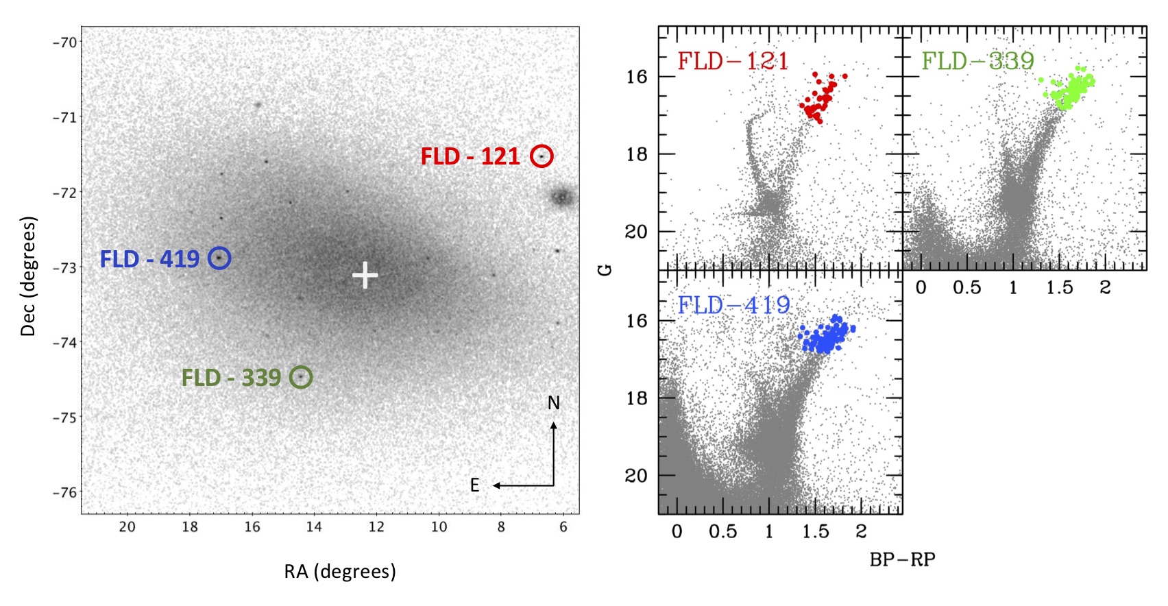
Figure 1: Left panel: spatial distribution of the three fields observed with FLAMES (marked as red, green and blue circles for FLD-121, FLD-339 and FLD-419, respectively) superimposed to the map of the SMC RGB stars with G between 16 and 19 from Gaia EDR3 (Gaia Collaboration et al., 2021), revealing the SMC old spheroid. The white plus symbol marks the position of the SMC centre derived by Ripepi et al. (2017). Right panel: Gaia EDR3 CMDs of the three SMC fields (grey points, Gaia Collaboration et al., 2021) with superimposed the spectroscopic GIRAFFE targets (same colours of left panel). In the CMD of FLD-121 is clearly visible the main sequence of the MW GC 47 Tucanae.

The adopted GIRAFFE-MEDUSA setups are HR11, with a spectral resolution of 24200 and ranging from 5597 to 5840 Å  and HR13, with a spectral resolution of 22500 and a spectral coverage between 6120 and 6405 Å . These two setups allow us to measure lines of the main groups of elements, like odd-Z (Na), $\alpha$ (O, Mg, Si, Ca and Ti), iron-peak (Sc, V, Fe, Ni, Cu) and s-process elements (Zr, Ba, La). The UVES fibers have been allocated to targets belonging to the three GCs and discussed in separated papers (Dalessandro et al., 2016, A. Minelli et al., in prep.). Table 1 lists the exposure times and the number of individual exposures for each setup and field.

Table 1: Coordinates of the FLAMES pointing, number of exposures and exposure times for the two FLAMES setups, adopted colour excess (Schlafly & Finkbeiner, 2011) and the number of SMC stars analysed in this work.

Field	RA	Dec	HR11	HR13	E(B-V)	$N_{SMC}$
	(J2000)	(J2000)			(mag)
FLD-121	00:26:49.0	–71:32:09.9	7x2700sec	5x2700sec	0.028	37
			1x2200sec
FLD-339	00:57:48.9	–74:28:00.1	9x2700sec	5x2700sec	0.042	78
FLD-419	01:08:17.7	–72:53:02.7	6x2700sec	4x2700sec	0.089	91

The spectroscopic targets for each field have been originally selected from near-infrared ($K_{s}$,J-${\rm K_{s}}$) CMDs, using the SofI@NTT catalogues for the region within 2.5 arcmin from the cluster centres (Mucciarelli et al., 2009, for NGC 339 and NGC 419, and unpublished proprietary photometry for NGC 121), and the 2MASS database (Skrutskie et al., 2006) for the external regions. The targets have been selected according to the following criteria: (1) stars fainter than the RGB Tip (${\rm K_{s}}$=12.62, Cioni et al., 2000); (2) stars brighter than ${\rm K_{s}}$= 14 for FLD-339 and FLD-419, and brighter than ${\rm K_{s}}$= 14.4 for FLD-121, in order to guarantee a signal-to-noise ratio (SNR) per pixel larger than $\sim$30 in both setups and in all the observed fields. Due to the paucity of RGB stars in the SMC outskirts, a fainter (by $\sim$0.4 mag) threshold has been adopted for FLD-121 in order to enlarge the number of observed SMC stars; (3) stars without close stars brighter than $<K_{s}^{star}+$1.0 within 2” ; (4) for the targets from the 2MASS catalogue (the majority of the observed targets) only stars with J and ${\rm K_{s}}$ magnitudes flagged as A (photometric uncertainties smaller than 10%) have been selected.

All the targets have been recovered in the Gaia EDR3 catalog. Right panel of Fig. 1 shows the position in the (G, BP-RP) CMDs of the observed targets considered as SMC stars according to their radial velocity (RV), see Section 3.3. Table 2 lists for all the SMC targets coordinates and the Gaia EDR3 identification number.

Table 2: Information about the SMC spectroscopic targets: ID for our internal catalogues, ID and coordinates from Gaia EDR3 (Gaia Collaboration et al., 2021), measured RV, derived atmospheric parameters and [Fe/H] abundance ratio. The entire table is available in electronic form.

ID	ID Gaia EDR3	RA	Dec	RV	$\rm T_{\rm eff}$	$\log{\rm g}$	${\rm v_{\rm t}}$	[Fe/H]
		(degree)	(degree)	(km s-1)	(K)	(cgs)	(km s-1)	(dex)
FLD-121_23	4689857932203222528	6.6427941	-71.5293047	144.3$\pm$ 0.2	4115	0.79	1.8	–1.58$\pm$ 0.10
FLD-121_24	4689857863486443520	6.6292441	-71.5407885	146.9$\pm$ 0.1	4140	0.80	1.8	–1.40$\pm$ 0.11
FLD-121_50	4689845798923576704	6.7124313	-71.5774614	123.5$\pm$ 0.1	4319	1.06	1.7	–1.01$\pm$ 0.13
FLD-121_51	4689857691687749888	6.6839449	-71.5429782	150.8$\pm$ 0.3	4234	1.05	1.7	–1.56$\pm$ 0.14
FLD-121_100004	4689848036601043584	7.0469194	-71.4811913	123.6$\pm$ 0.1	4142	0.80	1.8	–0.93$\pm$ 0.10
FLD-121_100086	4689845597059733248	6.7120893	-71.5895200	106.2$\pm$ 0.1	4065	0.84	1.8	–0.89$\pm$ 0.11
FLD-121_100175	4689859787631565056	7.0625549	-71.4769602	121.1$\pm$ 0.2	4375	0.98	1.7	–1.32$\pm$ 0.13
FLD-121_100185	4689858172724094720	6.4880274	-71.5481267	140.2$\pm$ 0.1	4084	0.88	1.8	–1.17$\pm$ 0.10
FLD-121_100211	4689852189834915072	6.2466252	-71.5899642	133.0$\pm$ 0.2	4345	1.09	1.7	–1.14$\pm$ 0.14
FLD-121_100237	4689844978584591104	6.4954253	-71.6527985	150.8$\pm$ 0.1	4293	1.12	1.7	–0.82$\pm$ 0.13
FLD-121_100263	4689843363676630528	7.1153070	-71.6019383	137.3$\pm$ 0.1	4132	0.84	1.8	–1.01$\pm$ 0.10
FLD-121_100272	4689846730930989440	6.9812926	-71.5614137	170.8$\pm$ 0.1	4029	0.63	1.8	–0.98$\pm$ 0.10
FLD-121_100330	4689859031717528576	6.5997764	-71.4819327	139.3$\pm$ 0.3	4424	1.09	1.7	–1.75$\pm$ 0.17
FLD-121_100335	4689862914367958144	6.4217566	-71.4335678	131.3$\pm$ 0.1	4194	0.93	1.7	–0.99$\pm$ 0.13
FLD-121_100365	4689851266416720768	6.2102084	-71.6388781	145.3$\pm$ 0.1	4093	0.63	1.8	–1.09$\pm$ 0.10
FLD-121_100382	4689842569108117888	7.1356396	-71.6152387	121.9$\pm$ 0.1	4088	0.70	1.8	–1.24$\pm$ 0.11
FLD-121_100440	4689842161085790080	7.0699869	-71.6558040	129.8$\pm$ 0.3	4488	1.14	1.7	–1.25$\pm$ 0.17

The spectra have been reduced with the dedicated ESO GIRAFFE pipeline, including bias-subtraction, flat-fielding, wavelength calibration with a standard Th-Ar lamp and spectral extraction. The contribution of the sky has been subtracted from each spectrum by using a median sky spectrum, as obtained by combining $\sim$15-20 spectra from fibres allocated to sky positions within each exposure. The final SNR per pixel of the spectra is of $\sim$30-50 for HR11 spectra and $\sim$40-60 for HR13 spectra. Fig. 2 shows, as an example of the spectral quality, the spectra of two SMC giant stars with very similar atmospheric parameters and a large ($\sim$1.5 dex) difference in [Fe/H].

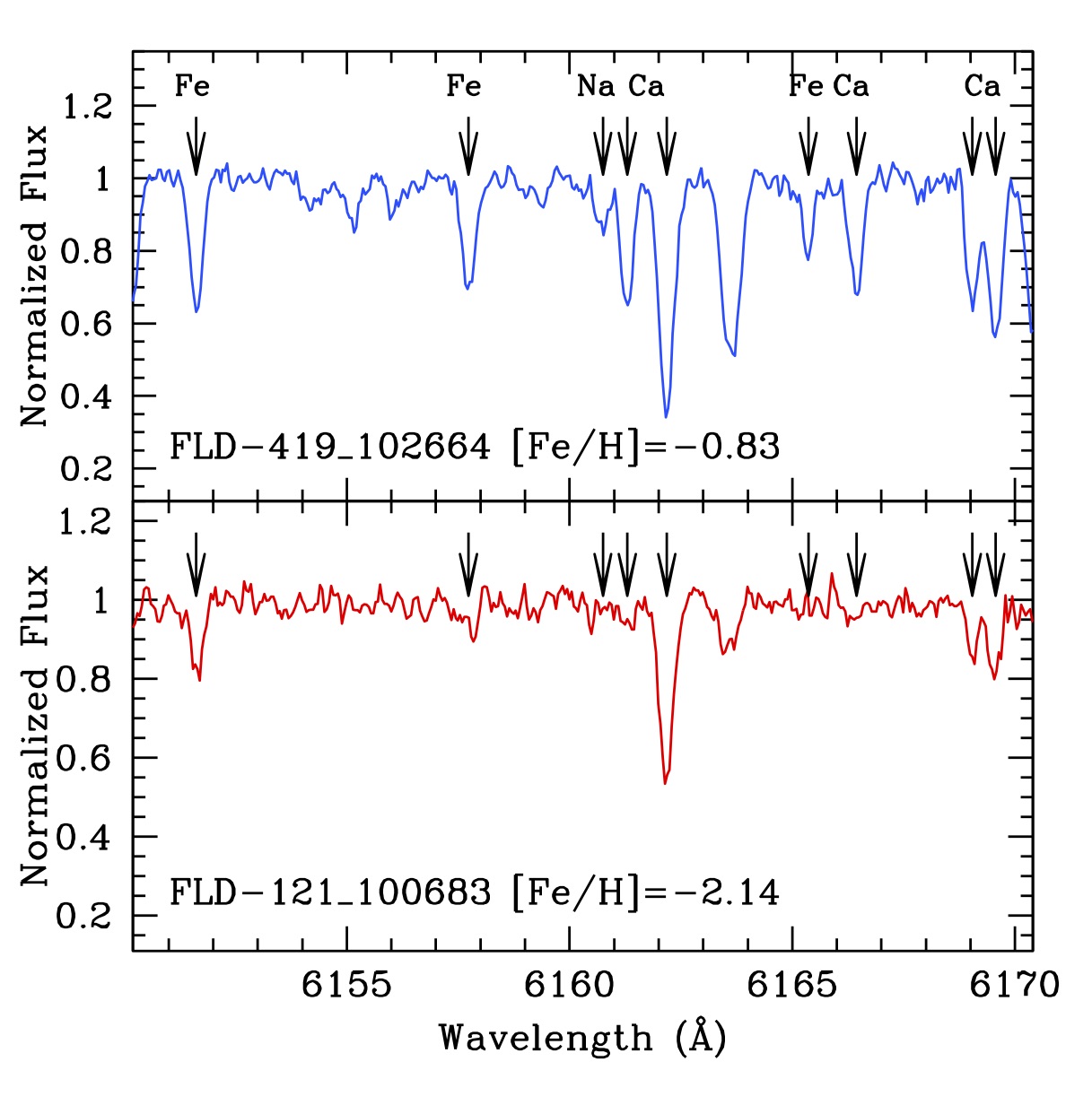
Figure 2: Comparison between the HR13 spectra of the stars FLD-419_102664 (upper panel) and FLD-121_100683 (lower panel). The stars have very similar atmospheric parameters but different iron content. Arrows mark the position of some metallic lines of interest.

2.2 MW control sample

As discussed in Minelli et al. (2021), the comparison between chemical abundances obtained from different works can be hampered by various systematics characterising the chemical analyses, for instance the method used to infer the stellar parameters, the adopted atomic data for the analysed transitions, model atmospheres and solar reference abundances. For this reason, when chemical analyses of extra-galactic stars are performed (with the aim to compare their abundances with those of MW stars), it is crucial to consider also a control sample of MW stars analysed in an homogeneous way, in order to erase the main systematics quoted above and highlight and quantify possible differences and similarities between the abundance ratios of stars from different galaxies.

We defined a control sample of MW stars analysed with the same assumptions used for the SMC stars. We analysed five MW GCs covering the same metallicity range of the SMC stars ([Fe/H] between $\sim$–2.2 and $\sim$–0.5 dex) and for which FLAMES spectra obtained with the GIRAFFE HR11 and HR13 setups are available in the ESO archive (ID programs: 072.D-0507 and 083.D-0208, PI: Carretta). The selected GCs are NGC 104, NGC 1851, NGC 1904, NGC 4833 and NGC 5904. The use of the same GIRAFFE setups allows us to derive chemical abundances in these MW GCs from the same transitions used for the SMC stars. We restrict the analysis only to the stars with effective temperatures and surface gravities comparable with those of the SMC stars studied here six stars for NGC 104, 2 for NGC 1851, 6 for NGC 5904, 3 for NGC 1904 and 4 for NGC 4833. Only for O and Na that exhibit large star-to-star variations in each of these GCs, we analysed stars belonging to the so-called first population and selected according to Carretta et al. (2009). The O and Na abundances of these first population stars can be considered as a good proxy of the chemical composition of the MW field at those metallicities.

3 Spectral analysis

3.1 Line selection

We selected for each star an appropriate set of unblended metallic lines, selected by visual inspection of suitable synthetic spectra. The latter have been calculated with the code SYNTHE (Sbordone et al., 2004; Kurucz, 2005), using the typical atmospheric parameters of the observed stars (see Section 3.2), adopting ATLAS9 model atmospheres (Castelli & Kurucz, 2004) and including all the atomic and molecular transitions in the Kurucz/Castelli linelist. The synthetic spectra have been convoluted with Gaussian profiles in order to reproduce the observed line broadening, mainly dominated by the instrumental resolution. We privileged transitions with laboratory oscillator strengths. Only for the Sc II line at 6245.6 Å  , for the Si I lines at 6155.1 and 6237.3 Å , and for the Cu I line at 5782 Å we adopted solar oscillator strengths.

Because the level of blending of a given transition depends on the metallicity, in this case not known a priori, we adopted an iterative process to define the linelist of each target.

A preliminary linelist has been defined by adopting a metallicity [M/H]=–1.0 dex for all the used synthetic spectra, according to the mean metallicity of the SMC derived from previous studies (Carrera et al., 2008; Dobbie et al., 2014a, b; Parisi et al., 2016; Nidever et al., 2020). After a first chemical analysis, a new set of unblended lines has been defined for each star using a synthetic spectrum calculated with the appropriate chemical composition. This procedure has been specifically necessary for the most metal-poor stars of our sample, with [Fe/H] significantly lower than the mean value of [Fe/H]=–1.0 dex, and for a few stars with enhancement of s-process elements. The average number of selected metallic lines is of about 80-90 for most of the stars (with [Fe/H]$\sim$–1.0 dex), decreasing down to 40-50 for the most metal-poor ones. Most of the lines used in the metal-poor stars are still available for metal-rich stars, while some features are excluded because saturated or blended with other lines at higher metallicities. However, we checked that the use of different samples of lines depending on the stellar metallicity does not introduce biases in the abundances at different metallicities.

All the used lines are listed in Table 3 together with the corresponding log gf and excitation potential $\chi$.

Table 3: List of the used transitions together with oscillator strengths, the excitation potential and the reference of the atomic data. Wavelengths without some decimal digits indicate transitions affected by hyperfine/isotopic splitting. The entire table is available in electronic form.

Wavelength	Ion	loggf	$\chi$	Reference
(Å )			(eV)
5590.720	Co I	-1.870	2.042	Fuhr et al. (1988)
5598.480	Fe I	-0.087	2.521	Fuhr & Wiese (2006)
5601.277	Ca I	-0.523	2.526	Smith & Raggett (1981)
5611.356	Fe I	-2.990	3.635	Fuhr et al. (1988)
5615.644	Fe I	0.050	3.332	Fuhr & Wiese (2006)
5618.632	Fe I	-1.276	4.209	Fuhr & Wiese (2006)
5624.542	Fe I	-0.755	3.417	Fuhr & Wiese (2006)
5633.946	Fe I	-0.320	4.991	Fuhr & Wiese (2006)
5638.262	Fe I	-0.840	4.220	Fuhr & Wiese (2006)
5647.234	Co I	-1.560	2.280	Fuhr et al. (1988)
5648.565	Ti I	-0.260	2.495	Martin et al. (1988)
5650.689	Fe I	-0.960	5.085	Fuhr & Wiese (2006)
5651.469	Fe I	-2.000	4.473	Fuhr et al. (1988)
5652.318	Fe I	-1.920	4.260	Fuhr & Wiese (2006)
5653.867	Fe I	-1.610	4.386	Fuhr & Wiese (2006)
5661.345	Fe I	-1.756	4.284	Fuhr & Wiese (2006)
5662.516	Fe I	-0.573	4.178	Fuhr & Wiese (2006)
5670.8**	V I	-0.420	1.081	Martin et al. (1988)
5679.023	Fe I	-0.900	4.652	Fuhr & Wiese (2006)
5682.633	Na I	-0.706	2.102	NIST

3.2 Atmospheric parameters

The derived atmospheric parameters are listed in Table 2. Effective temperatures ($\rm T_{\rm eff}$) and surface gravities ($\log{\rm g}$) have been estimated from the photometry. In particular, $\rm T_{\rm eff}$ have been obtained from the broad-band colour $(\rm G-K_{s})_{0}$ adopting the $(\rm G-K_{s})_{0}$-$\rm T_{\rm eff}$ transformation provided by Mucciarelli, Bellazzini & Massari (2021). We adopted G magnitudes from Gaia EDR3 and ${\rm K_{s}}$ from 2MASS. G magnitudes have been corrected for extinction following the prescriptions by Gaia Collaboration et al. (2018), while ${\rm K_{s}}$ magnitudes adopting the extinction coefficient by McCall (2004). The colour excess values E(B-V) are from the infrared dust maps by Schlafly & Finkbeiner (2011) and listed in Table 1.

Uncertainties in $\rm T_{\rm eff}$ have been estimated by propagating for any individual star the errors in the adopted colour and in the colour excess. The typical error in the $(\rm G-K_{s})_{0}$colours is of about 0.03-0.05 mag, dominated by the uncertainty of the ${\rm K_{s}}$ magnitude, and translating in 20-40 K of uncertainty in $\rm T_{\rm eff}$ . For the colour excess, we adopted a conservative error of 0.01 mag for all the three fields, despite the lower errors quoted by Schlafly & Finkbeiner (2011), leading to a negligible (a few K) uncertainty in $\rm T_{\rm eff}$ . These uncertainties have been added in quadrature to the typical error associated to the $(\rm G-K_{s})_{0}$-$\rm T_{\rm eff}$ transformation (46 K), estimated as 1$\sigma$ dispersion of the fit residuals (Mucciarelli, Bellazzini & Massari, 2021), and that dominates the total $\rm T_{\rm eff}$ error (typically $\sim$50-60 K).

The $\log{\rm g}$ values have been calculated through the Stefan-Boltzmann relation adopting the photometric $\rm T_{\rm eff}$, a true distance modulus $(m-M)_{0}$=18.965$\pm$0.025 (Graczyk et al., 2014), the bolometric corrections by Andrae et al. (2018) and a stellar mass of 1.0$M_{\odot}$. Concerning the distance modulus, it is worth to recall that the SMC has a substantial line-of-sight depth, not easy to properly take into account for each individual target. According to the depth maps provided by Subramanian & Subramaniam (2009), the three fields studied in this study should cover a depth range between 2 and 6 kpc. Considering a conservative variation of the distance by 3 kpc increases the quoted uncertainties in log g only by 0.02 dex, translating in variations of less of less than 0.02 in the abundances of single ionised (but without impact on the abundances of neutral lines). Uncertainties in log g are of the order of 0.1, including the uncertainties in $\rm T_{\rm eff}$  distance modulus and stellar mass. The final error budget in log g is dominated by the uncertainty in the stellar mass, assumed to be $\pm$0.2 $M_{\odot}$, reflecting the possible spread in ages of our targets (older than $\sim$1-2 Gyr). Microturbulent velocities (${\rm v_{\rm t}}$) are usually derived spectroscopically by erasing any trend between iron abundance and the reduced equivalent widths (defined as the logarithm of the EW normalised to the wavelength). Because of the relatively small number ($\sim$30-40 or less) of available Fe I lines in the adopted spectral ranges, ${\rm v_{\rm t}}$ obtained spectroscopically risk to be uncertain or unreliable. In order to avoid significant fluctuations in ${\rm v_{\rm t}}$ (with an impact on the derived abundances), we adopted the $\log{\rm g}$ - ${\rm v_{\rm t}}$ relations provided by Mucciarelli & Bonifacio (2020) and based on the spectroscopic ${\rm v_{\rm t}}$ obtained from high-resolution, high-SNR spectra of giant stars in 16 Galactic GCs. The uncertainty in ${\rm v_{\rm t}}$ has been estimated by adding in quadrature the error arising from the uncertainty in $\log{\rm g}$ and that of the adopted $\log{\rm g}$ - ${\rm v_{\rm t}}$ relation and is of the order of 0.2 km s^-1 .

3.3 Radial velocities

RVs have been measured by using the code DAOSPEC (Stetson & Pancino, 2008) that performs a line fitting assuming a Gaussian profile. The code is automatically launched by using the software 4DAO (Mucciarelli, 2013) that allows us a visual inspection of all the fitted lines in order to directly evaluate the quality of the fitting procedure. RVs have been measured by the position of about 100 metallic lines for each star. The internal uncertainty of the RV for each spectrum is estimated as the standard error of the mean, of the order of 0.1-0.3 km/s. The final RV for each target is obtained as the weighted mean of the values obtained from the two setups. The accuracy of the wavelength calibration has been checked by measuring the position of the strong emission sky line at 6300.3 Å in the HR13 setup, finding no significant offset. No sky emission lines are available in the HR11 setup and we cannot directly check the accuracy of the wavelength calibration. However, the RVs obtained from the two setups agree each other with an average difference between RV from HR11 and HR13 of +0.12$\pm$0.06 km s^-1($\sigma$= 0.8 km s^-1). This excludes any offset for the two setups and confirming the accuracy also of the RVs from HR11 spectra.

3.4 Chemical abundances

The chemical abundances of Na, Mg (from the line at 5711 Å), Si, Ca, Ti, Fe, Ni and Zr have been derived from the measure of the equivalent widths (EWs) of unblended lines by using the code GALA (Mucciarelli et al., 2013). EWs have been measured by using the code DAOSPEC (Stetson & Pancino, 2008).

For species whose lines are affected by blending (O and the Mg lines at 6318-19 Å ) or by hyperfine/isotopic splitting (Sc, V, Cu, Ba and La), abundances have been derived using our own code SALVADOR that performs a $\chi^{2}$-minimisation between the observed lines and a grid of synthetic spectra calculated on-the-fly with the code SYNTHE (Sbordone et al., 2004) and including all the atomic and molecular lines available in the Kurucz/Castelli linelists. For all the species investigated, when the lines are not clearly detectable, we provide upper limits based on the comparison between observed and synthetic spectra.

The [OI] line at 6300 Å can be also contaminated by telluric lines, depending on the stellar RV. This possible contamination has been checked with suitable synthetic spectra of the Earth atmosphere calculated with the TAPAS tool (Bertaux et al., 2014). These synthetic spectra are calculated assuming the appropriate date of observation and airmass of our targets, in order to account for the proper weather conditions of the observations. In case of contamination, the line profile has been cleaned by dividing the observed spectrum by the telluric one and visually checking that no discontinuities were introduced. Fig. 3 shows an example of a stellar spectrum around the [OI] line before and after the telluric correction.

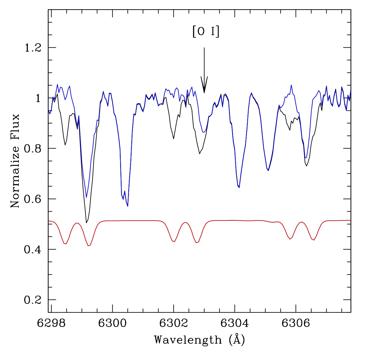
Figure 3: Example of the telluric correction around the [O I] line in the star FLD-339_466: black curve is the original (not corrected for RV) spectrum, the blue curve is the spectrum corrected for the telluric lines and the red one is the synthetic spectrum of the Earth atmosphere (shifted for sake of clarity).

In the calculation of the synthetic spectra used to measure the oxygen abundance, the Ni abundance of each star has been included to account for the blending of the O feature with a Ni line.

Mg abundances have been obtained for most of the stars from the EW of the line at 5711 Å . As discussed in Minelli et al. (2021), this transition is heavily saturated for giant stars with [Fe/H] $>$ –1.0 dex. For the latter stars, the Mg triplet at 6318-19 Å should be preferred because these lines are still sensitive to the Mg abundance. Therefore, for the stars for which the Mg line at 5711 Å turns out to be saturated, the Mg abundance has been derived from the Mg triplet using spectral synthesis in order to include the contribution of the close auto-ionization Ca line.

Finally, only for the Na lines used here (5682-88 Å and 6154-60 Å ) we corrected the derived abundances for departures from the LTE assumption applying the corrections by Lind et al. (2011).

The abundances are referred to the solar ones, taking as reference the values from Grevesse & Sauval (1998), apart from oxygen for which the adopted value is from Caffau et al. (2011).

3.5 Abundance uncertainties

In the determination of the uncertainties in each derived abundance ratio we take into account two main sources of error, namely the errors arising from the measurement procedure (EW or spectral synthesis) and those arising from atmospheric parameters.

(1) Uncertainties related to the measurement procedure are computed as the dispersion of the mean normalised to the root mean square of the number of used transitions. Properly, this term includes both uncertainties from line fitting and from adopted log gf values. For the elements measured from the EWs and for which only one line is available, the DAOSPEC uncertainty associated to the Gaussian fitting procedure (corresponding to 1$\sigma$ of the fit residuals) is assumed as internal error. For the elements (O and La) for which only one transition has been measured using spectral synthesis, the internal error has been estimated by means of Monte Carlo simulations, creating a sample of 500 synthetic spectra with a Poissonian noise that reproduces the observed SNR and repeating the line-fitting procedure. The dispersion of the abundance distribution obtained from these noisy synthetic spectra is assumed as 1$\sigma$ uncertainty.
(2) Uncertainties due to atmospheric parameters have been estimated by repeating the analysis by varying each time a given parameter of the corresponding 1$\sigma$ error and keeping fixed the other parameters.

These two sources of uncertainties have been added in quadrature. Since the abundance of the species X is expressed as abundance ratios [X/Fe], also the uncertainties in the Fe abundance have been taken into account. The final errors in [Fe/H] and [X/Fe] abundance ratios are calculated as follows:

$$\sigma_{[Fe/H]}=\sqrt{\frac{\sigma_{Fe}^{2}}{N_{Fe}}+(\delta^{\rm T_{\rm eff}}_{Fe})^{2}+(\delta^{log\leavevmode\nobreak\ g}_{Fe})^{2}+(\delta^{\rm v_{\rm t}}_{Fe})^{2}}$$ (1)

$$\begin{split}&\sigma_{[X/Fe]}=\\ &\sqrt{\frac{\sigma_{X}^{2}}{N_{X}}+\frac{\sigma_{Fe}^{2}}{N_{Fe}}+(\delta^{\rm T_{\rm eff}}_{X}-\delta^{\rm T_{\rm eff}}_{Fe})^{2}+(\delta^{log\leavevmode\nobreak\ g}_{X}-\delta^{log\leavevmode\nobreak\ g}_{Fe})^{2}+(\delta^{\rm v_{\rm t}}_{X}-\delta^{\rm v_{\rm t}}_{Fe})^{2}}\end{split}$$ (2)

where $\sigma_{X,Fe}$ is the dispersion around the mean of the chemical abundances, $N_{X,Fe}$ is the number of lines used to derive the abundances and $\delta^{i}_{X,Fe}$ are the abundance variations obtained modifying the atmospheric parameter i.

3.6 Abundances of the MW control sample

Table 4 lists the average abundance ratios, together with the standard deviation and the average uncertainty in the abundance ratio, for the 5 GCs of the MW control sample. We compared the atmospheric parameters and [Fe/H] of the analysed stars with those by Carretta et al. (2009) and Carretta et al. (2014) that analysed the same spectroscopic dataset. The average differences between our analysis and the literature ones are +52$\pm$11 K ($\sigma$= 50 K) for $\rm T_{\rm eff}$ , –0.01$\pm$0.01 ($\sigma$= 0.03) for log g, +0.07$\pm$0.04 km s^-1($\sigma$= 0.19 km s^-1) for ${\rm v_{\rm t}}$ and –0.03$\pm$0.02 dex ($\sigma$= 0.07 dex) for [Fe/H].

Table 4: Average abundance ratios, the corresponding standard deviation and the average uncertainty for the five GCs of the MW control sample.

Ratio	NGC 104		NGC 1851		NGC 5904		NGC 1904		NGC 4833
	$<>$	$\sigma$	$<>$	$\sigma$	$<>$	$\sigma$	$<>$	$\sigma$	$<>$	$\sigma$	$<\sigma_{[X/Fe]}>$
[Fe/H]	–0.84	0.02	–1.15	0.03	–1.29	0.01	–1.57	0.04	–2.11	0.03	0.07
[O/Fe]	+0.42	0.04	+0.40	0.03	+0.47	0.04	+0.54	0.04	+0.59	0.03	0.08
[Na/Fe]	+0.00	0.03	–0.15	0.04	–0.35	0.04	–0.40	0.03	–0.50	0.05	0.08
[Mg/Fe]	+0.31	0.04	+0.34	0.04	+0.33	0.03	+0.35	0.04	+0.38	0.02	0.10
[Si/Fe]	+0.28	0.03	+0.26	0.05	+0.28	0.02	+0.30	0.06	+0.46	0.06	0.11
[Ca/Fe]	+0.29	0.04	+0.25	0.03	+0.26	0.03	+0.25	0.01	+0.26	0.06	0.09
[Sc/Fe]	+0.35	0.03	+0.17	0.04	+0.26	0.05	+0.13	0.03	+0.28	0.04	0.08
[Ti/Fe]	+0.24	0.02	+0.06	0.01	+0.16	0.03	+0.15	0.01	+0.20	0.06	0.09
[V/Fe]	+0.19	0.04	–0.15	0.03	–0.06	0.05	–0.05	0.03	–0.09	0.03	0.10
[Ni/Fe]	–0.04	0.02	–0.10	0.04	–0.11	0.03	–0.08	0.02	–0.11	0.04	0.06
[Cu/Fe]	–0.02	0.04	–0.41	0.02	–0.37	0.05	–0.52	0.03	–0.60	0.04	0.08
[Zr/Fe]	+0.30	0.04	+0.11	0.03	+0.10	0.03	+0.14	0.06	+0.06	0.06	0.12
[Ba/Fe]	+0.04	0.05	+0.13	0.04	+0.08	0.06	+0.10	0.04	+0.31	0.05	0.12
[La/Fe]	+0.29	0.03	+0.35	0.05	+0.24	0.04	+0.14	0.03	+0.27	0.06	0.08

4 RV and [Fe/H] distributions

4.1 RV distribution

According to previous spectroscopic studies (Harris & Zaritsky, 2006; Carrera et al., 2008; Dobbie et al., 2014a; De Leo et al., 2020; Hasselquist et al., 2021) we identified as members of the SMC those stars with RV between +80 and +250 km s^-1. The membership is confirmed also by the proper motions measured from Gaia EDR3 (Gaia Collaboration et al., 2021). We exclude from the chemical analysis stars members of the GC associated to each field (these stars will be discussed in a forthcoming paper of the series), stars with spectra contaminated by prominent TiO or $C_{2}$ molecular bands or with too low SNR. The final sample discussed in this work includes a total of 206 stars out of the 320 observed stars. The RV and [Fe/H] for this sample are listed in Table 2. Fig. 4 and  5 shows the RV and [Fe/H] discrete and kernel density distributions of the three SMC fields. The advantage of the latter representation is that the distribution is independent of the choice of the bin width and of the starting bin, at variance with the discrete distributions.

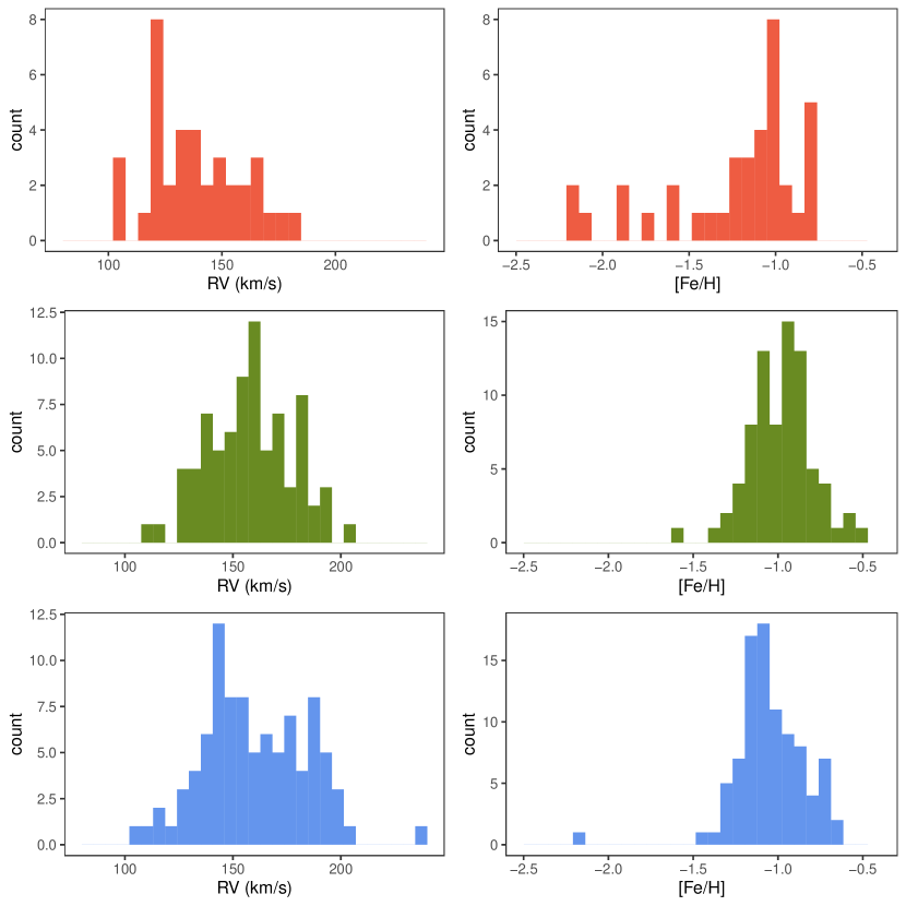
Figure 4: RV and [Fe/H] distributions (left and right panel, respectively) of the three fields. Colours indicate the different fields: FLD-121 (red), FLD-339 (green) and FLD-419 (blue).

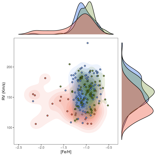
Figure 5: RVs are plotted against [Fe/H] for target stars in the central panel of the figure. Colour-shaded areas denote the contours of the three clusters RV vs [Fe/H] distributions. Side plots show the kernel distributions of the RV (right-hand panel) and the [Fe/H] values (top panel) for each cluster. Same colours of Fig. 4

.

The RV distributions of the three fields appear significantly different with each other, both in terms of the main peak and shape. The RV distribution of FLD-121 peaks at RV$\approx$+125 km s^-1 , that of FLD-339 displays a peak at RV$\approx$+160 km s^-1 , while that of FLD-419 exhibits two distinct peaks, the main one at $\approx$+150 km s^-1 and the second one at $\approx$+180 km s^-1 . A Kolmogorov-Smirnov test performed on these distributions confirms that the RV distributions of FLD-339 and FLD-419 are significantly different with respect to that of FLD-121 (with statistic significance larger than 99.9%), while we cannot reject the hypothesis that FLD-339 and FLD-419 may derive from the same population.

The differences in the peak of these three RV distributions are compatible with the rotation pattern of the SMC as inferred from low-resolution spectroscopic surveys of giant stars (Dobbie et al., 2014a; De Leo et al., 2020), from the HI column density map (Di Teodoro et al., 2019) and from the APOGEE results from 17th Data Release of the Sloan Digital Sky Survey (Abdurro’uf et al., 2022). All these studies show that the western side of the SMC, where FLD-121 is located, has a lower velocity with respect to the eastern side. However, the presence of multiple peaks, clearly visible in the distribution of FLD-419, seems to suggest a more complex kinematic pattern (as discussed below).

4.2 [Fe/H] distribution

The [Fe/H] distribution of the entire sample is peaked at [Fe/H]$\sim$–1.0 dex, with about 95% of the stars having [Fe/H] between –1.5 and –0.5 dex and with a weak but extended metal-poor tail reaching [Fe/H]$\sim$–2.2 dex. This distribution is qualitatively similar to those obtained from low-resolution spectra using Ca II triplet (Carrera et al., 2008; Dobbie et al., 2014a; Parisi et al., 2016) and that from APOGEE data (Nidever et al., 2020). However, similar to what we see with the RV distributions, when the individual fields are considered, the metallicity distributions appear different with each other. The distributions of FLD-339 and FLD-419 are confined between –1.5 and –0.5 dex, with only one star per field ($\sim$1%) with [Fe/H]$<$–1.5 dex . On the other hand the distribution of FLD-121 ranges from –0.8 dex down to –2.2 dex, with $\sim$20% of the stars more metal-poor than –1.5 dex. Note that the APOGEE field 47Tuc, superimposed to our field FLD-121, exhibits a lower fraction of metal-poor stars, $\sim$2%, probably reflecting some selection bias against metal-poor stars in the APOGEE observations.
The peaks of the distributions of FLD-339 and FLD-419 are separated by $\sim$0.2 dex and located at [Fe/H]$\sim$–0.9 and $\sim$–1.1 dex, respectively. Also, the two distributions seem to be not symmetric, with the presence a secondary peak at [Fe/H]$\sim$–1.1 dex in FLD-339 and a heavily-populated metal-rich tail or a secondary peak in FLD-419 (see Sec. 4.5).

4.3 [Fe/H] distribution and the age-metallicity relation

We try to interpret the derived [Fe/H] distributions in terms of ages, using as a guidance the SF histories recovered from Hubble Space Telescope (Noel et al., 2007; Sabbi et al., 2009; Cignoni et al., 2012, 2013) and ground-based (Massana et al., 2022) photometry, and the theoretical age-metallicity relations available for the SMC (Pagel & Tautvaisiene, 1998; Tsujimoto & Bekki, 2009; Cignoni et al., 2013).

All these works agree that the early epochs of the SMC have been characterised by a significant SF activity followed by a long quiescent period, interrupted between $\sim$3 and $\sim$4 Gyr ago by significant SF episodes, likely due to some merger events. The oldest SMC GC, NGC 121, has an age of $\sim$10.5$\pm$0.5 Gyr (Glatt et al., 2008) and a metallicity of [Fe/H]$\sim$–1.2/–1.3 dex (Dalessandro et al., 2016, A. Minelli et al. in prep.). This suggests that the SF activity in the first Gyrs was able to increase the metallicity to values as high as [Fe/H]$\sim$–1.2/–1.3 dex. We can consider the SMC field stars in our sample with [Fe/H]$<$–1.3 dex (which are almost all located in FLD-121) as formed in the first 1-2 Gyr of the life of the galaxy.

The subsequent evolution of the SMC and the corresponding metallicity distribution can be interpreted in the light of the theoretical age-metallicity relations: Fig. 6 shows that by Pagel & Tautvaisiene (1998) assuming a burst of SF at an age of $\sim$4 Gyr. After a long period characterised by a low SF efficiency (and where the metallicity remains almost constant), the SF in the SMC re-ignites with a prominent burst, likely triggered by the first close encounter between SMC and LMC (Bekki et al., 2004; Bekki & Chiba, 2005). The most recent SF history for the SMC provided by Massana et al. (2022) using the SMASH photometry identified the re-ignition of the SF at $\sim$3.5 Gyr ago, simultaneously in both the Clouds. The stars with [Fe/H]$>$–1.3 dex analysed here should be a mixture of stars with different ages (from $\sim$1 to $\sim$10-11 Gyr). It is not easy to separate the different populations in terms of age due to the almost constant [Fe/H] over a large age range. Massana et al. (2022) identified in the SF history of the SMC five peaks (at $\sim$3, 2, 1, 0.45 Gyr ago and one still ongoing) occurring simultaneously also in the LMC. A fascinating possibility is that the different peaks in the metallicity distributions of FLD-339 and FLD-419 could be associated to some of these different bursts of SF. Finally, we can suppose that the stars with [Fe/H] around –0.6/–0.5 dex are likely formed with the burst at 1 Gyr. This is confirmed also by the metallicities of the stellar clusters with ages around 1 Gyr (see e.g. Parisi et al., 2022)

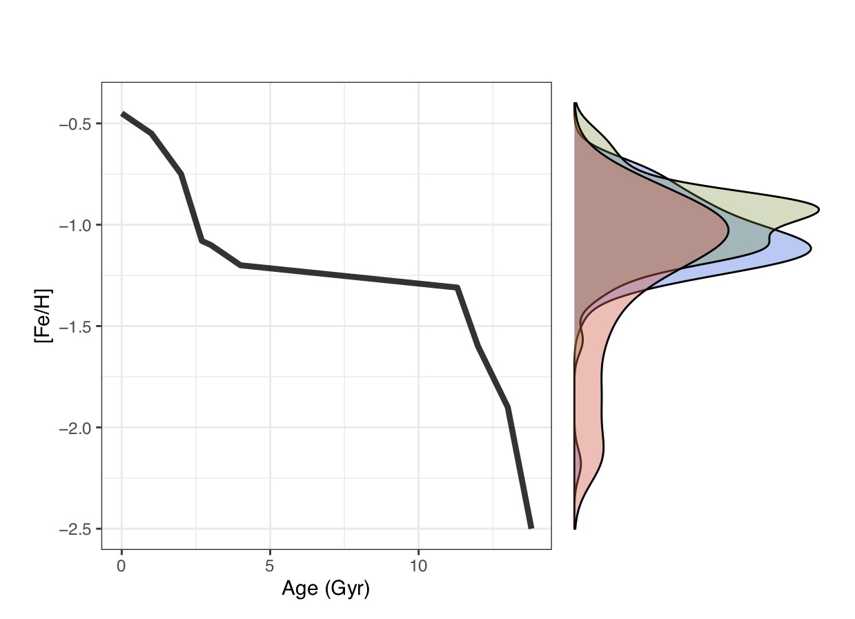
Figure 6: Main panel: age-metallicity relation by Pagel & Tautvaisiene (1998). Side panel: the kernel [Fe/H] distributions for the individual SMC field stars discussed in this work.

4.4 Run of [Fe/H] with the distance

Previous spectroscopic studies (Carrera et al., 2008; Dobbie et al., 2014a; Parisi et al., 2016; Choudhury et al., 2020; Grady et al., 2021) found evidence of a shallow (from –0.03 to –0.07 dex/deg) metallicity gradient, within 3^∘–5^∘. Fig. 7 shows the run of [Fe/H] of the spectroscopic targets with their projected distance from the SMC centre (Ripepi et al., 2017). The mean metallicity in three fields is consistent with the shallow gradient previously proposed by Choudhury et al. (2020). However two main differences between the external field FLD-121 and the two internal ones are evident. First, in FLD-121 the fraction of metal-poor stars ([Fe/H]$<$–1.5 dex) is about $\sim$20%, against $\sim$1% in the other two fields. The fraction of metal-poor stars increases outward reflecting a larger fraction of old stars with respect to those formed subsequently during the long quiescent period and the recent SF bursts and that are preferentially confined in the innermost region of the SMC (see e.g. Rubele et al., 2018).

Second, in the metallicity distribution of FLD-121 there is a clear lack of stars with [Fe/H] between –0.8 and –0.5 dex, instead detected in FLD-339 and FLD-419. Following the discussion above, these stars should have $\sim$1 Gyr (the youngest stars among the intermediate-age SMC populations). Again, this is consistent with a scenario where the younger, metal-richer populations are progressively more concentrated toward the innermost regions. Age-metallicity gradients of this kind are quite common in dwarf galaxies (see e.g. Taibi et al., 2022, and references therein).

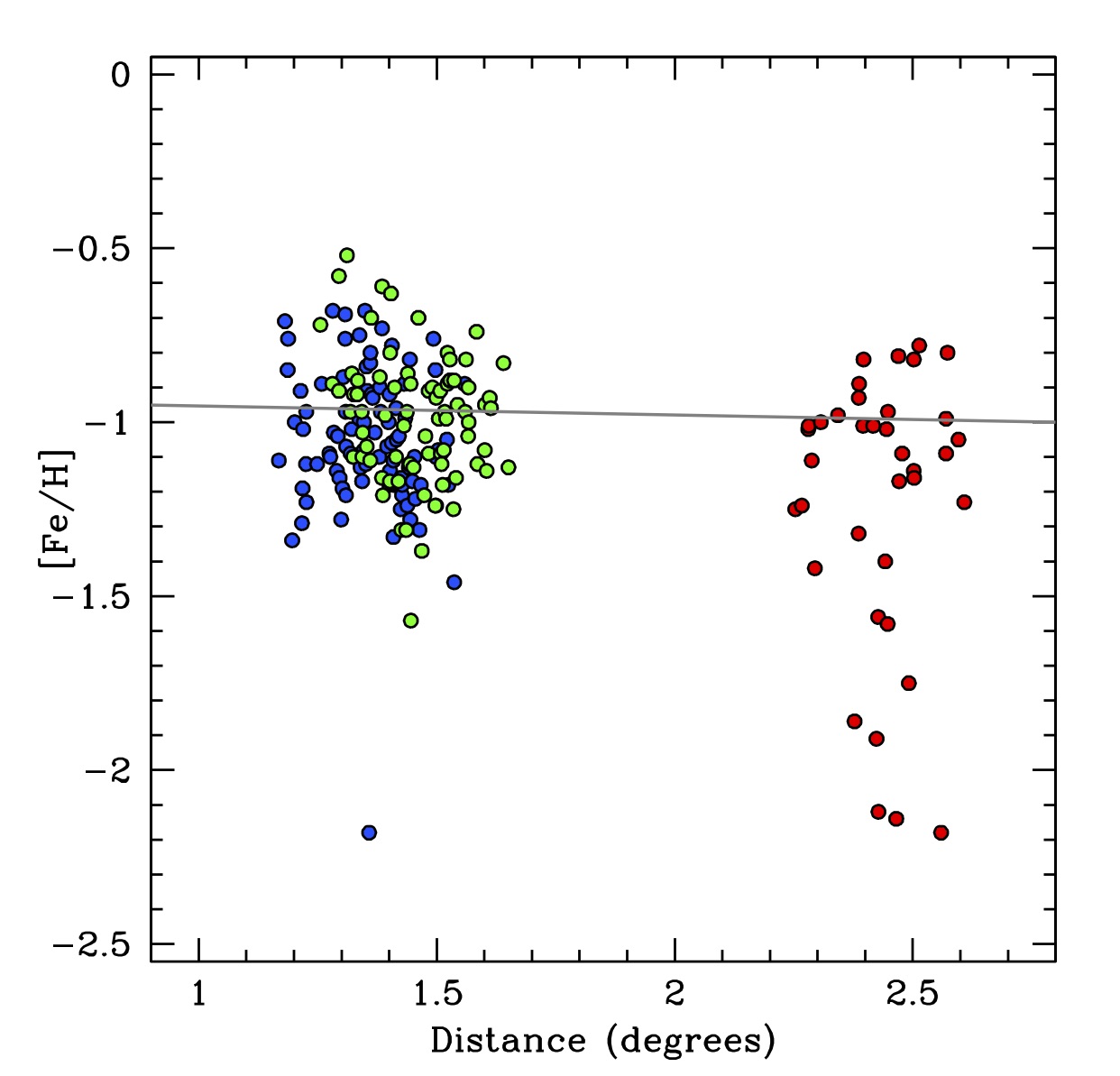
Figure 7: Behaviour of [Fe/H] as a function of the projected distance from the SMC centre (Ripepi et al., 2017), same colours of Fig. 1. The thick grey line is the linear fit for the metallicity gradient estimated by Choudhury et al. (2020).

4.5 Possible kinematic/chemically distinct sub-structures?

The distribution of the SMC stars in the RV-[Fe/H] plane seems to suggest the presence of sub-structures, in particular the two different peaks of the [Fe/H] distribution of FLD-339, the large and asymmetric [Fe/H] distribution of FLD-419 and the double-peak of the RV distribution of FLD-419.

We used the gaussian mixture package Mclust (Scrucca et al., 2016), within the R environment, to analyse the distribution of FLD-339 and FLD-419 stars in the [Fe/H] - RV space. Mclust choose the best model, both in terms of number and form (e.g., equal or variable variance, orientation etc., see Scrucca et al., 2016) of the gaussian components, by means of the Bayesian Information Criterion. Since we are interested in substructures within the bulk of the metallicity distribution we exclude from the analysis the two metal-poor outliers, one per field. While for FLD-339 a single elliptical gaussian model is the preferred solution, the [Fe/H] - RV distribution of FLD-419 is best described with two elliptical gaussian components with the same variance both in [Fe/H] and RV. The gain of this model with respect to a single elliptical gaussian is only marginal, in practice they provide an equally good representation of the data. Still, the solution synthesise the properties of the hypothesised two components. The first component has ($\mu_{\mathrm{[Fe/H]}}$, $\mu_{\mathrm{RV}}$)= ( -0.85 dex, 171.8 km s^-1), and it accounts for 33% of the sample, the second component has ($\mu_{\mathrm{[Fe/H]}}$, $\mu_{\mathrm{RV}}$)= ( -1.13 dex, 154.5 km s^-1), accounting for the remaining 67% of the sample. The standard deviations are $\sigma_{\mathrm{[Fe/H]}}$= 0.10 dex, and $\sigma_{\mathrm{RV}}$= 22.7 km s^-1. It seems that the most metal rich component has a larger systemic RV than its metal-poor counterpart.

As additional check, we performed a Kolmogorov-Smirnov test on the RV sub-populations of FLD-419, separated according to the metallicity of their member stars (and assuming [Fe/H]=–1.05 dex as a boundary between the two groups of stars). We obtained that the two RV distributions cannot be extracted from the same population with a significance of 98%.

The size of the FLD-419 sample is not sufficient to put this odd result on sound statistical bases, still it may be suggestive of the presence of some chemo-kinematic substructures in the SMC along this line of sight. In this respect, it is worth recalling that the SMC has a substantial line-of-sight depth, depending on the used tracers and ranging from a few kpc up to about 20 kpc (see e.g. de Grijs & Bono, 2015; Subramanian et al., 2017). Therefore, when we observe stars in an individual SMC field we are likely crossing different depths and we are sampling different populations in terms of kinematics and metallicity.

5 Chemical abundance ratios

We derived abundances of Na, O, Mg, Si, Ca, Sc, Ti, V, Fe, Ni, Cu, Zr, Ba and La for 206 SMC RGB stars. All the abundances, with the corresponding uncertainties, are available in the electronic form (Table 5). With respect to the APOGEE sample by Hasselquist et al. (2021) we measured a larger number of species, in particular Na, Sc, Ti, V, Cu, Zr, Ba and La, not included in that study. Fig. 8-11 show the behaviour of derived abundance ratios as a function of [Fe/H] for the analysed SMC stars, highlighting stars belonging to the different fields. These abundance ratios are compared with those obtained for the control sample of 5 Galactic GCs, adopting the same assumptions in the chemical analysis and therefore removing most of the systematics of the analyses. This comparison allows us to highlight the real difference between SMC and MW stars of similar [Fe/H]. Additionally, we show abundance ratios for Galactic field stars from the literature as reference. The comparison with the literature is affected by the systematics among the different analyses (in terms of model atmospheres, solar abundance values, NLTE corrections, linelists, use of dwarf and giant stars). However, it is useful to display the overall trends in the MW based on a large number of stars. In the following, we refer to the MW control sample to quantify the main differences and similarities between MW and SMC stars.

5.1 Na

Sodium is mainly produced in massive stars during the hydrostatic C and Ne burning, with a strong dependence of its yields on the metallicity. Also, a smaller contribution is provided by asymptotic giant branch (AGB) stars. In Galactic stars (both in the control sample and in literature data), [Na/Fe] increases by increasing [Fe/H] until it reaches solar values around [Fe/H]$>$–1 dex. An offset is evident between the values in the control sample and in the literature, especially in the metal-poor regime and likely due to the different NLTE corrections. Top-left panel of Fig. 8 shows the distribution of [Na/Fe] of the observed targets. The bulk of the SMC stars exhibits sub-solar [Na/Fe] abundance ratios at any metallicities, with an average value of about –0.4/–0.5 dex, similar to the typical [Na/Fe] measured in the LMC stars (Van der Swaelmen et al., 2013; Minelli et al., 2021) but at higher [Fe/H]. The low [Na/Fe] values measured in the SMC stars may point to a lower contribution by massive stars, besides the larger impact of Type Ia supernovae (SNe Ia) at low metallicities in dwarf galaxies (Tolstoy et al., 2009). We observe a large scatter of [Na/Fe], not fully explainable within the typical uncertainties, and already detected in spectroscopic samples of LMC and SMC metal-rich stars (Pompéia et al., 2008; Van der Swaelmen et al., 2013; Minelli et al., 2021; Hasselquist et al., 2021). This scatter could reflect that multiple sites of Na production are taking place. Finally, we note a systematic difference between the median [Na/Fe] values in FLD-339 and FLD-419, where the latter displays [Na/Fe] higher by 0.1-0.15 dex. A systematic difference in [Na/Fe] of different regions of the parent galaxy has been also observed in the LMC (Van der Swaelmen et al., 2013) with the stars in the LMC bar more enriched in [Na/Fe] by 0.2 dex with respect to the LMC disc stars.

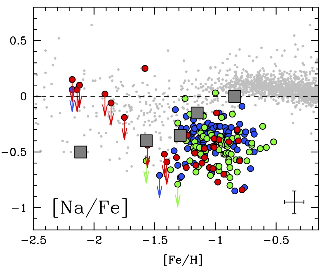
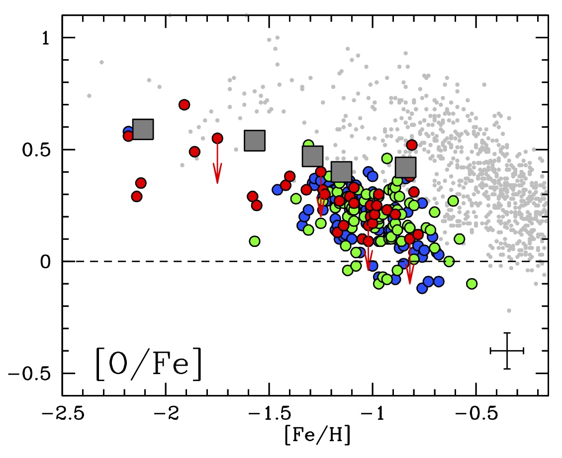
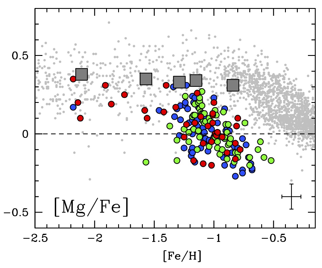
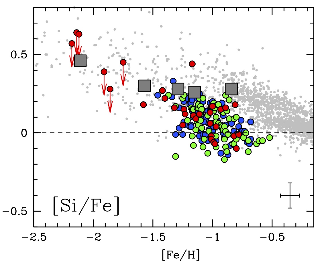
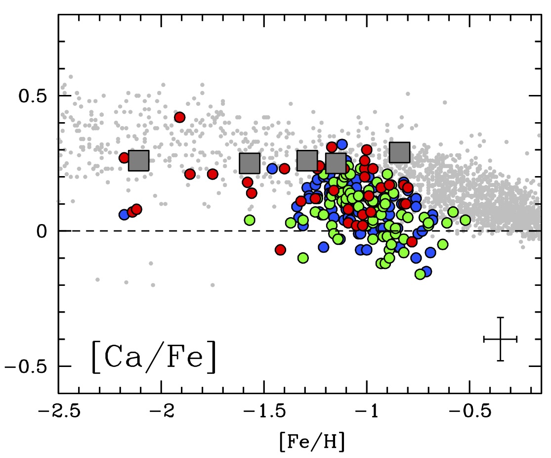
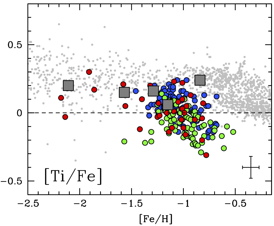
Figure 8: Behaviour of the light element [Na/Fe] and $\alpha$-elements [O/Fe], [Mg/Fe], [Si/Fe], [Ca/Fe] and [Ti/Fe] abundance ratios as a function of [Fe/H] for SMC stars located in the fields FLD-419, FLD-339 and FLD-121 (blue, green and red circles, respectively). Arrows indicate upper limits. The errorbars in the bottom-right corner indicate the typical uncertainties. Grey squares are the average values for the five Galactic GCs of the control sample. Abundances of Galactic stars from the literature are also plotted as a reference: Edvardsson et al. (1993); Gratton et al. (2003); Reddy et al. (2003, 2006); Bensby et al. (2005, 2014) for all the elements, Fulbright (2000); Stephens & Boesgaard (2002); Roederer et al. (2014) for Na, Mg, Si, Ca and Ti, Adibekyan et al. (2012) for Na, Mg, Si and Ca, Barklem et al. (2005) for Mg.

5.2 $\alpha$-elements

The $\alpha$-elements are produced mainly in short-lived massive stars exploding as core-collapse supernovae (CC-SNe), while a minor fraction (depending on the element) is synthesised in SNe Ia. Due to the time delay between the enrichment of the two classes of SNe, the [$\alpha$/Fe] abundance ratios are the classical tracers of the relative timescales of the different SNe. In particular, the metallicity of the knee (marking the onset of a significant chemical contribution by SNe Ia) can be used as a proxy of the SF efficiency of the galaxy (Tinsley, 1979; Matteucci & Greggio, 1986).

O and Mg (the so-called hydrostatic $\alpha$-elements) are produced mainly in stars with masses larger than $\sim$30-35 $M_{\odot}$ and without contribution by SNe Ia. On the other hand, Si, Ca and Ti (explosive $\alpha$-elements) are produced in less massive stars ($\sim$15-25 $M_{\odot}$) and with a smaller (but not negligible) contribution by SNe Ia (see e.g. Kobayashi et al., 2020b). Fig. 8 shows the behaviour with [Fe/H] of individual [$\alpha$/Fe] abundance ratios, while Fig. 9 shows the run of the average values of hydrostatic and explosive [$\alpha$/Fe]. These abundance ratios in the SMC stars clearly display a decrease by increasing the metallicity, moving from enhanced values for the most metal-poor stars ([Fe/H]$<$–1.5 dex) down to solar-scaled values in the dominant population. This trend is in contrast with that obtained by the APOGEE survey, where ”there is a slight increase in [Mg/Fe] beginning at [Fe/H]$\sim$–1.3 dex, with a peak at [Fe/H]$\sim$–1.0 dex, followed by a slight decrease. The [O/Fe], [Si/Fe] and [Ca/Fe] abundance patterns are flat over this range” (Hasselquist et al., 2021).

The most metal-poor stars in our sample exhibit enhanced values of [$\alpha$/Fe] and in agreement with the results by Nidever et al. (2020) and Reggiani et al. (2021) for SMC stars of similar metallicity. Oxygen and magnesium, that are mainly produced by stars with masses larger than $\sim$30 $M_{\odot}$, are, however, slightly underabundant at low [Fe/H] with respect to the MW sample, which points to a lower contribution from the most massive stars to the overall chemical enrichment of the SMC. The subsequent decrease of [$\alpha$/Fe] at higher [Fe/H] indicates that these stars formed from a gas enriched by SNe Ia. For stars with [Fe/H]$>$–1.5 dex the difference in [$\alpha$/Fe] between SMC and MW stars becomes more significant. In particular, the SMC-MW difference is more pronounced for hydrostatic $\alpha$-elements, again suggesting a lower contribution by stars with masses larger than 30-35 $M_{\odot}$ to the chemical enrichment of the SMC.

We note, as for Na, that the metal-rich stars in FLD-419 are slightly enhanced in [Ti/Fe], by $\sim$0.1 dex, with respect to the stars of the other two fields with similar [Fe/H].

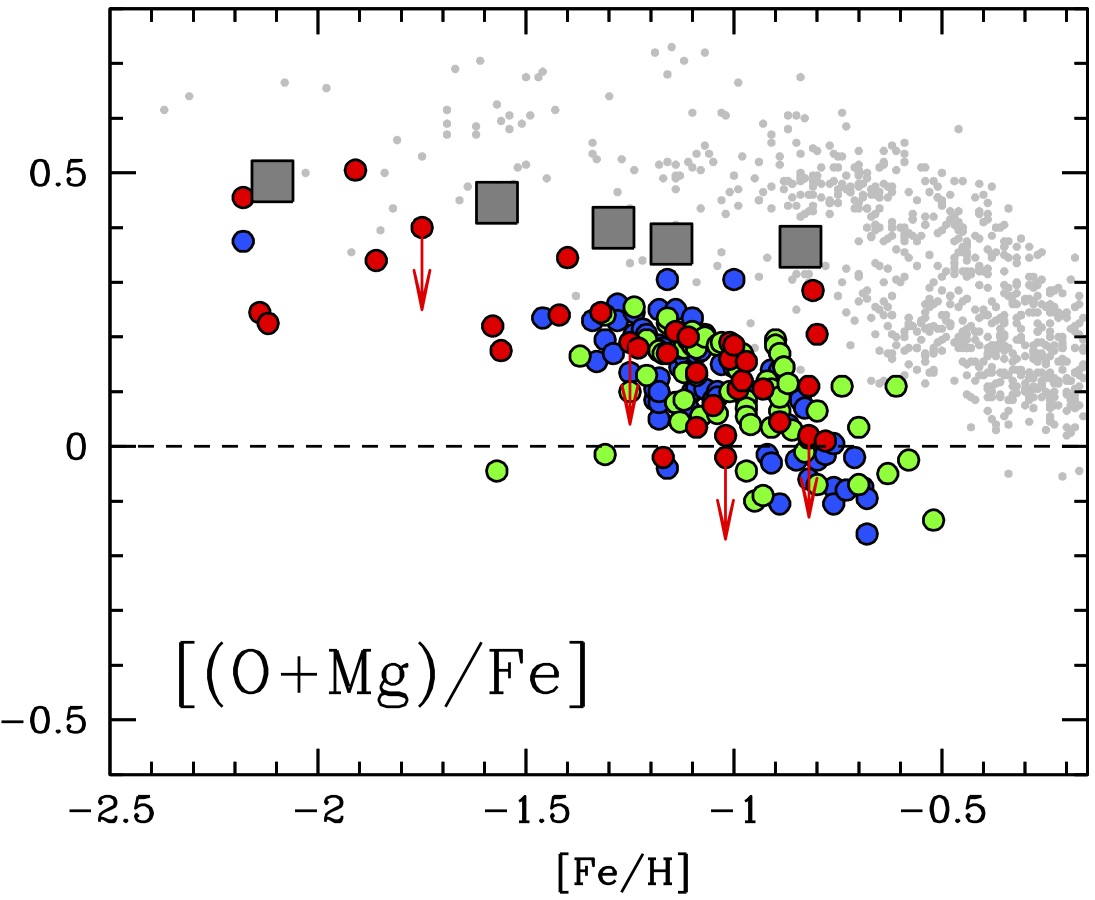
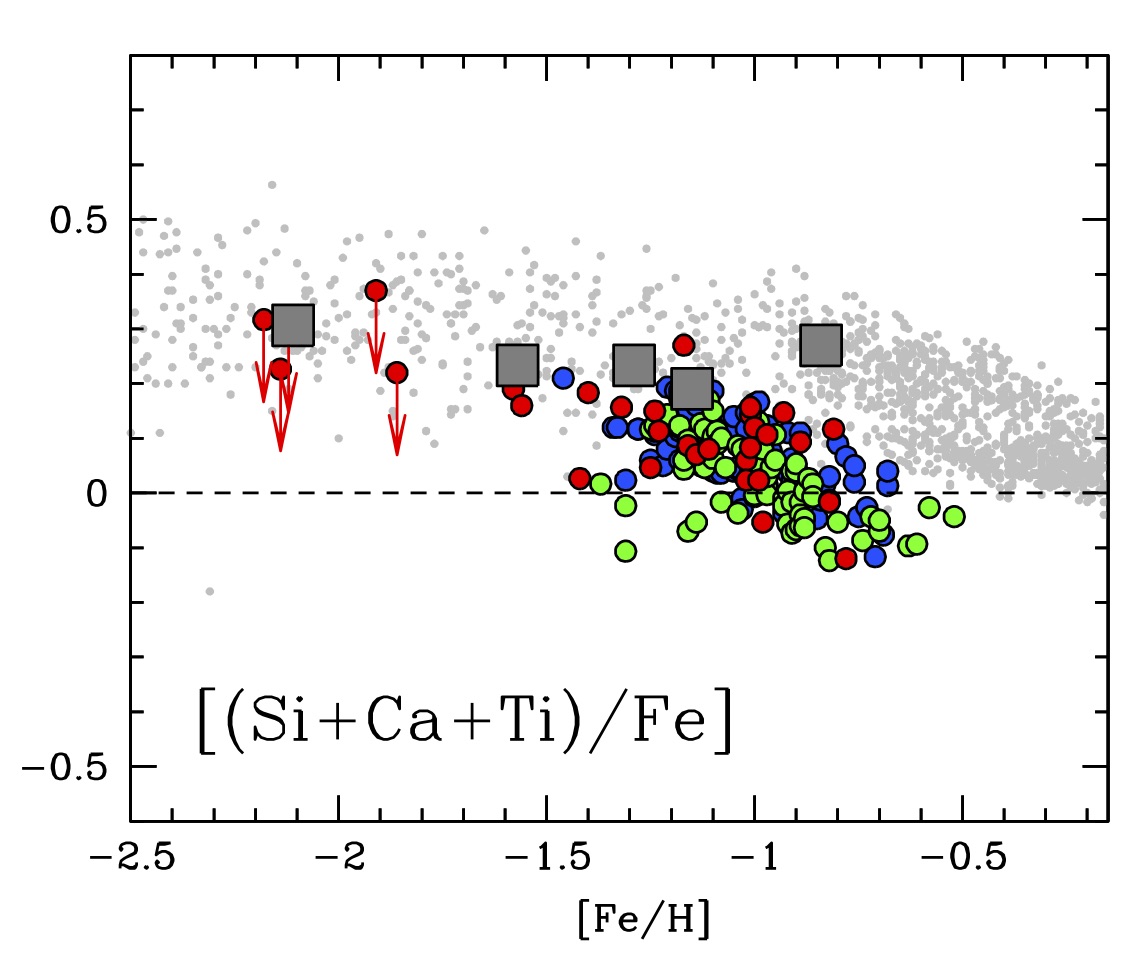
Figure 9: Behaviour of the hydrostatic and explosive average [$\alpha$/Fe] abundance ratios as a function of [Fe/H]. Same symbols of Fig. 8.

5.3 Iron-peak elements

Iron-peak elements are produced mainly in massive stars, through different nucleosynthesis paths (Limongi & Chieffi, 2003; Romano et al., 2010; Kobayashi et al., 2020b), and ejected in the interstellar medium both from normal CC-SNe and hypernovae. These elements are also partly produced by SNe Ia on longer time scales (Leung & Nomoto, 2018; Lach et al., 2020).

Sc and V are produced mainly in massive stars, with a small contribution by SN Ia only for V (Kobayashi et al., 2020b). The SMC stars with [Fe/H]$<$–1.5 dex have Sc and V abundances compatible with those measured in the control sample. We note some offsets between these abundance ratios in the control sample and in the literature data, likely attributable to different linelists (in terms of log gf and/or hyperfine structures. On the other hand, the metal-rich SMC stars have abundances of Sc and V significantly lower than the MW stars (see Fig. 10). For both elements, we observed a decrease of the abundance ratio with increasing [Fe/H] because of the overwhelming delayed contribution to Fe by SNe Ia. This behaviour resembles those observed in metal-rich stars of dwarf galaxies, like LMC and Sagittarius (see e.g. Sbordone et al., 2007; Minelli et al., 2021). We note that also [V/Fe] in metal-rich stars of FLD-419 is systematically higher by $\sim$0.15 dex with respect to the stars of FLD-339. A comparable shift has been detected also for [V/Fe] in the LMC disc and bar stars (Van der Swaelmen et al., 2013).

Ni is largely produced by SN Ia, with production also by CC-SNe, similar to the production of Fe. The SMC stars have [Ni/Fe] values compatible with those measured in the GCs of the control sample until [Fe/H]$\sim$–1.0 dex, while for higher metallicities this abundance ratio slightly decreases, reaching values around [Ni/Fe]$\sim$–0.2 dex (see Fig. 10). A similar behaviour in the SMC stars has been observed by Hasselquist et al. (2021). This mild trend resembles that observed for [Ni/Fe] in the LMC and in Sagittarius at higher [Fe/H] (Minelli et al., 2021). The decrease of [Ni/Fe] at higher metallicities is not observed in MW stars, where [Ni/Fe] remains constant. In this respect, Kobayashi et al. (2020a) suggested a lower contribution by sub-Chandrasekhar mass SN Ia to reproduce the [Ni/Fe] measured in dwarf spheroidal galaxies.
Cu is produced mainly in massive stars through the weak s-process (Romano & Matteucci, 2007), with a small contribution by AGB stars (Travaglio et al., 2004) and a negligible contribution by SN Ia (Iwamoto et al., 1999; Romano & Matteucci, 2007). The [Cu/Fe] abundance ratio in the SMC stars exhibits a large star-to-star dispersion and it is difficult to establish its real trend. However, it is clear that the most metal-rich SMC stars have [Cu/Fe] lower than that measured in MW stars, indicating again a lower contribution to the chemical enrichment by massive stars. Values of [Cu/Fe] lower than those measured in MW stars have been observed also in the LMC (Van der Swaelmen et al., 2013), Sagittarius (Sbordone et al., 2007) and Omega Centauri (Cunha et al., 2002).

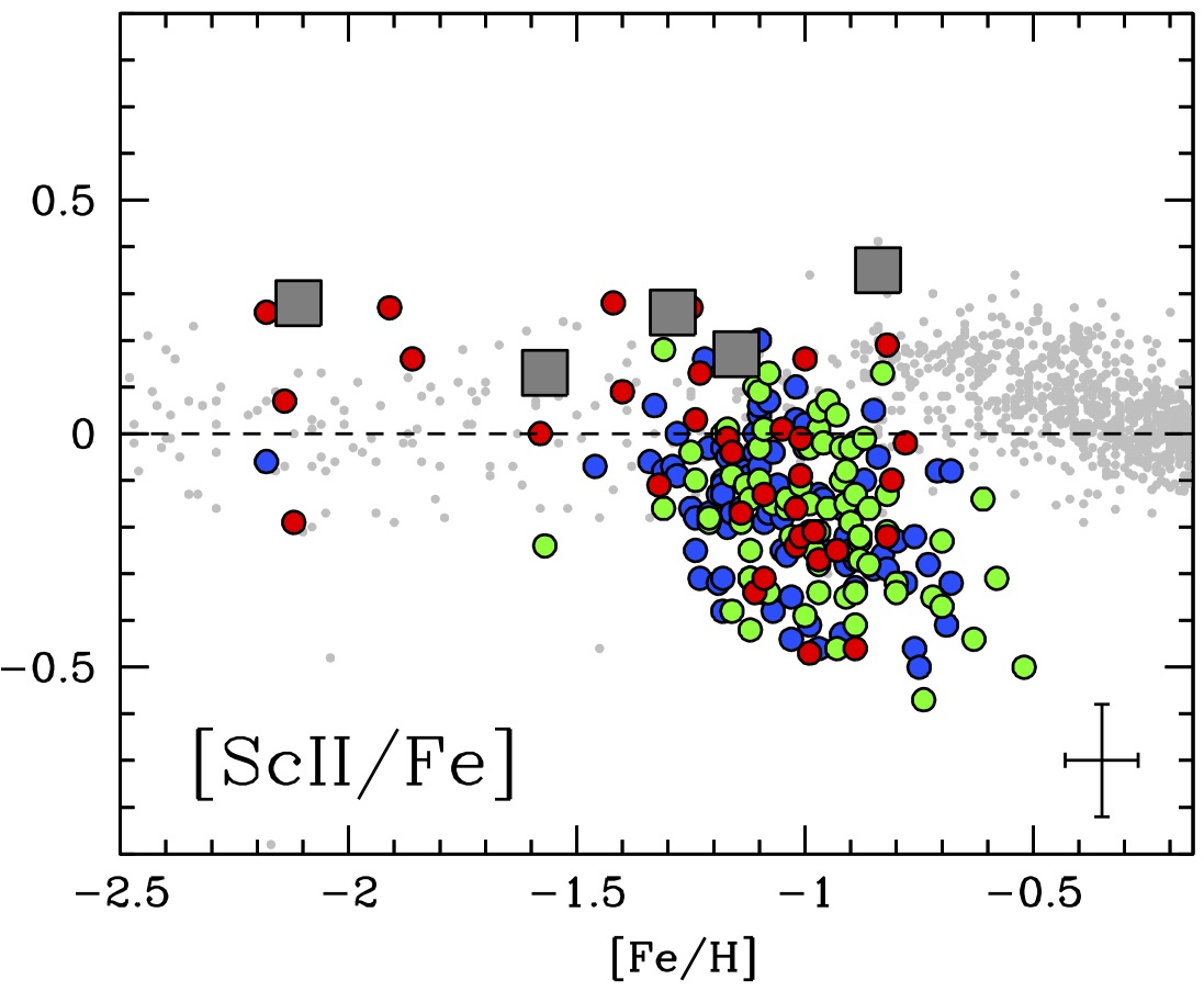
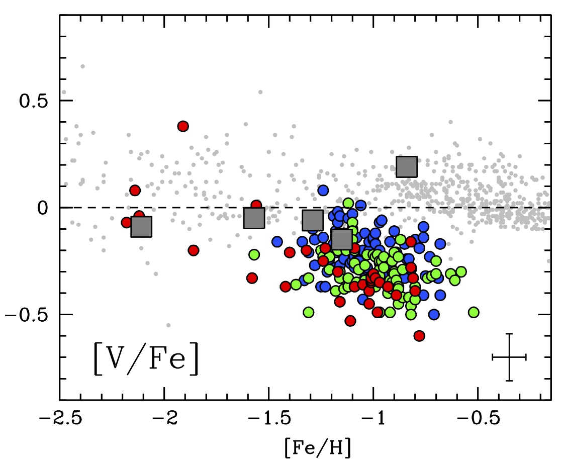
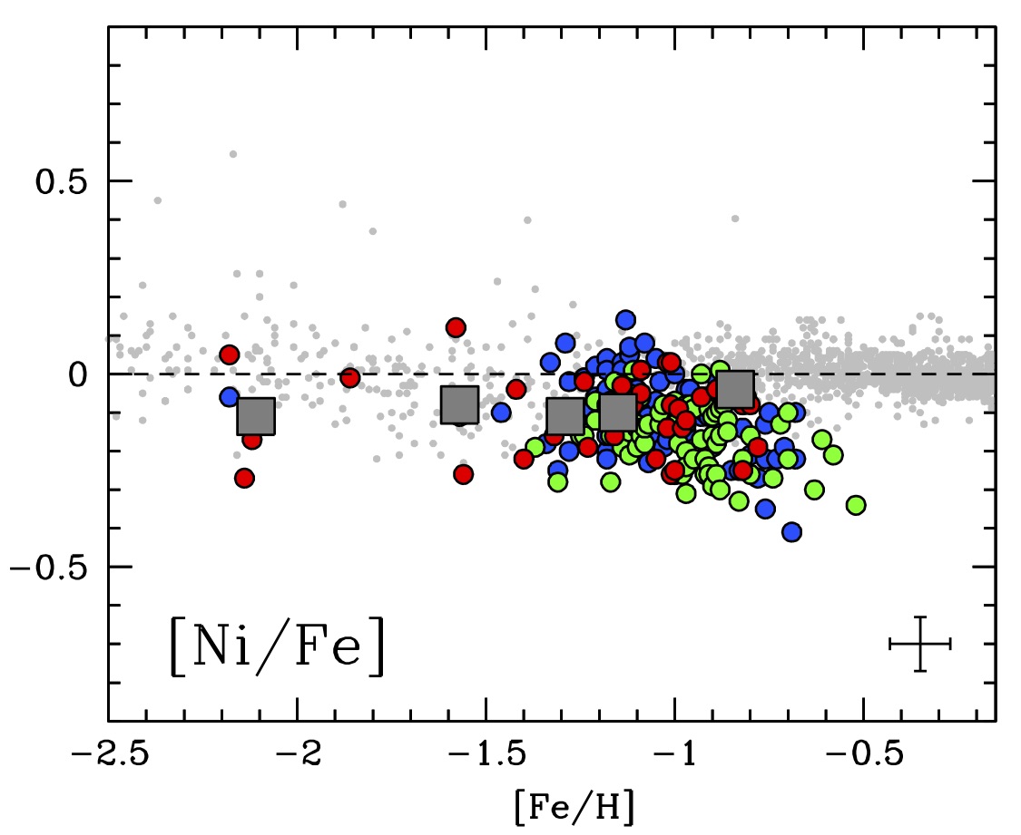
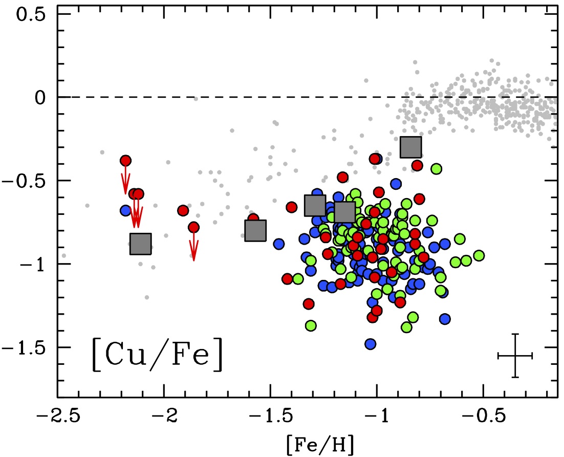
Figure 10: Behaviour of the iron-elements [Sc/Fe], [V/Fe], [Ni/Fe] and [Cu/Fe] abundance ratios as a function of [Fe/H]. Abundances of Galactic field stars are from Reddy et al. (2003, 2006); Roederer et al. (2014) for all the elements, Gratton et al. (2003) for Sc, V and Ni, Fulbright (2000) for V and Ni, Adibekyan et al. (2012) for Sc and Ni, Edvardsson et al. (1993); Stephens & Boesgaard (2002); Bensby et al. (2005) for Ni, Bihain et al. (2004); Yan et al. (2015) for Cu. Same symbols of Fig. 8.

5.4 Neutron capture elements

Elements heavier than the iron-peak group are produced through neutron capture processes on seed nuclei, followed by $\beta$ decays (Burbidge et al., 1957). The neutron capture elements measured here (namely Zr, Ba and La) are produced mainly by the slow process occurring in low-mass (1-3 M_⊙) AGB stars and in a minor amount in more massive stars (Busso et al., 1999; Cristallo et al., 2015). At low metallicities these elements are produced also through rapid processes (Truran, 1981), occurring in rare and energetic events like neutron star mergers or collapsars. In this spectroscopic dataset, there are no transition of pure r-process elements (i.e. Eu) and we cannot discuss the relative contribution of these two production channels. However, Reggiani et al. (2021) analysed 4 metal-poor SMC giant stars finding [Eu/Fe] values higher than those of the MW stars, supporting a strong contribution at these metallicities by r-process.

The SMC stars show [Zr/Fe] and [La/Fe] abundance ratios similar, within the star-to-star scatter, to those observed in MW stars, and slightly higher [Ba/Fe]. Generally, these results suggest that the enrichment by AGB stars in the SMC has been comparable to that in the MW. [Ba/Fe] in the SMC stars is enhanced ($\sim$+0.3/+0.4 dex) and higher than the values measured in the MW stars. [Ba/Fe] displays a large scatter at all the metallicities and not explainable in light of the typical uncertainties in the abundance ratios ($\sim$0.15 dex). At [Fe/H]$\sim$–1.0 dex, the SMC stars have values of [Ba/Fe] higher than those observed in the MW stars, suggesting a galaxy-wide initial mass function (IMF) biased in favour of the low-mass stars in the SMC. A similar behaviour is observed for [La/Fe], while [Zr/Fe] presents a trend in agreement with that observed for the MW. Similar to what we observe for Na and V, also for [Zr/Fe] we found a shift ($\sim$0.2 dex) between FLD-339 and FLD-419 that resemble those observed for the same ratio between LMC disc and bar stars (Van der Swaelmen et al., 2013). The high values of [Ba/Fa] and [La/Fe], together with the large star-to-star scatter, suggest that the production of s-process elements has been very efficient in the SMC, while the large star-to-star scatter could arise from enrichment from AGB stars of different metallicities, being the yields of AGB stars for these elements extremely metallicity-dependent.

Finally, we identified a few stars with high [Ba/Fe] and [La/Fe] values ($>$0.5-0.7 dex, reaching also +1.3 dex). A similar enhancement of s-process elements could be due to mass transfer processes from an AGB companion star in a binary system.

6 Conclusions

The analysis of optical spectra of 206 SMC RGB stars located in three different positions of the parent galaxy has allowed us to highlight some finer details of the complex and still poorly known nature of this galaxy. The main results are summarised as follows:

• The RV and [Fe/H] distributions of the three fields are different with each other. The fields FLD-339 and FLD-419, despite the same distance from the SMC centre, have [Fe/H] distributions peaked at different values, separated by 0.2 dex. These two populations could be connected to different bursts of SF occurring in the recent life of the SMC (Massana et al., 2022) or the result of a different chemical enrichment path in these regions (despite their similar projected distance from the SMC centre).

• The fraction of metal-poor ([Fe/H]$<$–1.5 dex) stars increases outward, being $\sim$1% in the two internal fields and $\sim$20% in FLD-121. This run likely reflects an age gradient in the SMC, with the internal regions dominated by intermediate-age, metal-rich stars and the outskirts by the old, metal-poor spheroid (see e.g. Rubele et al., 2018).

• The RV-[Fe/H] distribution of the observed fields seems to suggest the possible existence of chemically/kinematic distinct substructures. In particular, we potentially identified two groups of stars, one around [Fe/H]$\sim$–1.1 dex and RV$\sim$+154 km s^-1 and the other around [Fe/H]$\sim$–0.9 dex and RV$\sim$+172 km s^-1 . More data are needed to confirm the statistical significance of these chemo-kinematical substructures.

• The SMC displays, especially for the dominant, metal-rich component, distinct abundance patterns with respect to the MW stars. In particular, those elements mainly produced by massive stars (Na, $\alpha$, Sc, V and Cu) have abundance ratios lower than those measured in the MW stars. This suggests that the gas from which these stars formed has been poorly enriched by the most massive stars. This can be explained in light of the low SF rate expected for a galaxy as small as the SMC, leading to a lower contribution by massive stars to the overall chemical enrichment of the galaxy (Jeřábková et al., 2018; Yan et al., 2020). This is confirmed also by the most metal-poor stars of the sample that exhibit [O/Fe] and [Mg/Fe] ratios slightly lower than those in MW stars of similar [Fe/H].

• The [s/Fe] abundance ratios are enriched with respect to the MW stars, with a large star-to-star scatter, suggesting that these elements are produced by AGB stars of different masses and metallicities. Also, the enhancement of the [s/Fe] abundance ratios in the SMC seems to suggest a galaxy-wide IMF biased in favour of the low-mass stars in the SMC.

• The possibility that the IMF is not universal, but varies with the environment is the subject of lively debate (Bastian et al., 2010; Hopkins, 2018; Smith, 2020). Theoretically, if stars form in clusters according to IMFs that depend on the metallicity and density of the parent gaseous clumps, it is possible to calculate the integrated galaxy-wide IMF that in turn depends on the metallicity and star formation rate of the host galaxy (Jeřábková et al., 2018; Yan et al., 2020). Moreover, the abundance ratios of chemical elements produced in stars with initial masses falling in narrow and well-detached ranges can be used as powerful, indirect probes of the shape of the galaxy-wide IMF (e.g. Romano et al., 2017).

  Observationally, the possibility that the Sagittarius dwarf spheroidal galaxy had a stronger contribution from AGB stars to its chemical enrichment than the MW and the LMC is discussed in Hasselquist et al. (2021). Similarly, Hallakoun & Maoz (2021), resting on Gaia DR2 data, point to a bottom-heavy IMF for the Gaia-Enceladus progenitor. Finally, Mucciarelli et al. (2021) claim that the LMC GC NGC 2005 must have formed in an accreted system that experienced an extremely low star formation rate and, hence, an extremely low number of hypernova explosions, in order to explain the peculiarly low Zn abundance of the cluster.

  On the other hand, Hill et al. (2019) do not find any clear cut evidence in favour of a non-standard IMF in the Sculptor dwarf spheroidal galaxy. In a forthcoming paper, we will quantitatively deal with the issue of IMF variations in the SMC by computing chemical evolution models specifically tailored to this galaxy (Romano et al., in preparation).

• The three fields exhibit similar chemical patterns for all the elements but Na, V, Zr and Ti showing subtle differences among the fields. Differences in the same abundance ratios have been observed also in the LMC between bar and disk stars (Van der Swaelmen et al., 2013). These differences confirm that the chemical enrichment history in the SMC has been not uniform but depends on the position within the galaxy.

These promising results enforces the need to study the properties of the SMC stars locally rather than globally, with an effort to enlarge the samples of high-resolution spectra located in different regions of the galaxy. In this respect, the advent of the multi-object spectrographs like MOONS at the Very Large Telescope (Cirasuolo et al., 2020) and 4MOST at the VISTA Telescope (de Jong et al., 2019) will allow us a significant improvement in the investigation of possible chemically-distinct sub-structures in the Magellanic Clouds (Gonzalez et al., 2020).

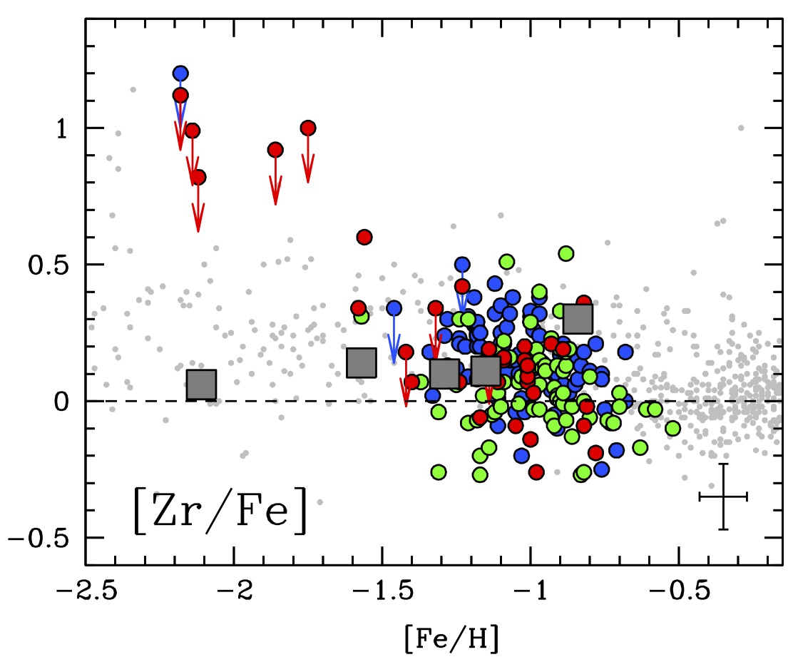
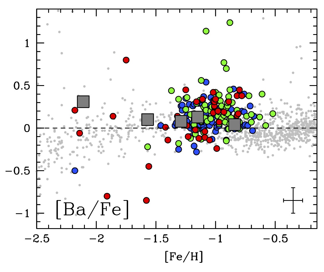
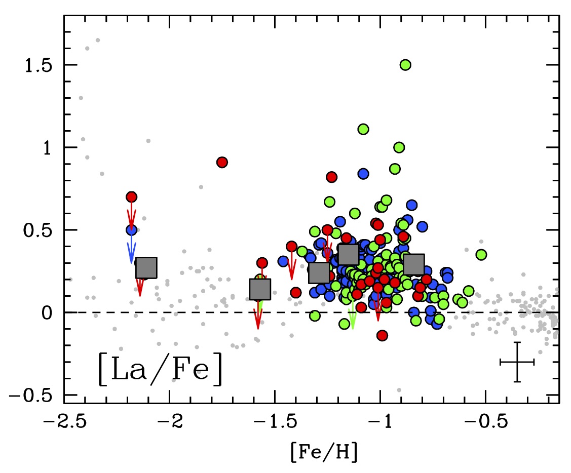
Figure 11: Behaviour of the neutron capture-elements [Zr/Fe], [Ba/Fe] and [La/Fe] abundance ratios as a function of [Fe/H]. Abundances of Galactic field stars are from Mishenina et al. (2013); Roederer et al. (2014) for all the elements, Edvardsson et al. (1993); Fulbright (2000); Reddy et al. (2003) for Zr and Ba, Burris et al. (2000); Battistini & Bensby (2016) for Zr and La, Stephens & Boesgaard (2002); Barklem et al. (2005); Bensby et al. (2005) for Ba.