Introducing Expertise Logic into Graph Representation Learning from A Causal Perspective

Abstract

Benefiting from the injection of human prior knowledge, graphs, as derived discrete data, are semantically dense so that models can efficiently learn the semantic information from such data. Accordingly, graph neural networks (GNNs) indeed achieve impressive success in various fields. Revisiting the GNN learning paradigms, we discover that the relationship between human expertise and the knowledge modeled by GNNs still confuses researchers. To this end, we introduce motivating experiments and derive an empirical observation that the GNNs gradually learn human expertise in general domains. By further observing the ramifications of introducing expertise logic into graph representation learning, we conclude that leading the GNNs to learn human expertise can improve the model performance. Hence, we propose a novel graph representation learning method to incorporate human expert knowledge into GNN models. The proposed method ensures that the GNN model can not only acquire the expertise held by human experts but also engage in end-to-end learning from datasets. Plentiful experiments on the crafted and real-world domains support the consistent effectiveness of the proposed method.

1 Introduction

As the improvement of machine computing capacity hits a developmental bottleneck, barely increasing the network parameters and the number of input data becomes challenging to boost the model performance. Therefore, researchers explore empowering the model’s capacity by leveraging human prior knowledge to guide optimization. An outstanding practical attempt is converting the natural data structures, e.g., images and videos, into derived discrete data structures, e.g., language and graph. Benefiting from the injection of human prior knowledge, derived discrete data structures are generally semantically dense. Thus, exploring the semantic information from such derived data can effectively improve the model performance.

By revisiting the learning paradigms of benchmark methods, we observe that the improvements according to GNNs essentially lie in two aspects: 1) the message passing process, which aggregates features from a node’s neighbors, e.g., GGAE [17], $p$-Laplacian GNN [6], PG-GNN [13], GloGNN [19]; 2) the readout function, which projects the node representations into the graph representation, e.g., Adaptive Structure Aware Pooling [28], Top-k Pool [8], SAG Pool [16], etc. State-of-the-art approaches elaborate GNN structures to learn discriminative representations from graphs. However, there exist several innate questions challenging current researchers who explore GNN-based learning paradigms: what kind of knowledge do GNNs capture from graphs and is such knowledge in accordance with human expertise?

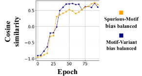
(a) Visualization of a conventional GNN approach’s learning degree of the expertise logic during optimization on benchmark datasets. We specifically measure the cosine similarity between the logits of the expert model and the GNN model. Generally, the results show that the similarity has an increasing trend with training.

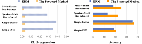
(b) Comparisons between the baseline, i.e., Empirical Risk Minimization (ERM), and the proposed method on various datasets. The left plot demonstrates the KL divergence between the features derived by the expert model and the candidate model. The right plot collects the classification performance of the compared methods. The empirical observations jointly support that our proposed method can better learn the expertise logic and consistently outperform the baseline.

Figure 1: The motivating explorations.

Inspired by this motivation, we intuitively introduce the experiments to explore the knowledge captured by GNNs. As demonstrated in Figure 1(a), the expertise logic contained by the expert model is continuously learned by the purely Connectionism-based data-driven GNN model, and we thus derive the intuition that GNNs indeed gradually capture the knowledge that is homogeneous to the human expertise during training. To further support the statement, we conduct experiments on various domains in Figure 1(b). Based on the empirical results, it can be observed that there is a general occurrence of GNNs learning human expertise to a certain extent across different tasks. The proposed approach, treating the expertise logic as guidance, can improve GNNs to learn human expertise and further boost the model performance. The observation leads to an empirical conclusion: introducing expertise logic into graph representation learning practically improves the model performance.

In light of such empirical finding, we propose the Causal Logic Graph Representation Learning, dubbed CLGL, to improve the model to learn the expertise logic that is causally related to the graph representation learning tasks. CLGL achieves the aforementioned objectives by enabling the GNN model to learn knowledge from higher-order causal models constructed based on expertise logic. We also conduct a theoretical analysis of CLGL based on the Structural Causal Model (SCM) [30, 24, 12], demonstrating its effectiveness. Moreover, we further incorporate the concept of interchange intervention from causal theory-related methods, enabling CLGL to facilitate a more comprehensive learning of expertise logic. The sufficient comparisons on various datasets, including the crafted and real-world datasets, support the consistent effectiveness of CLGL.

Contributions:

• We discover an intriguing observation, which leads to an empirical conclusion: introducing expertise logic into graph representation learning improves the model performance. Additionally, we undertake a thorough investigation, employing comprehensive theoretical analyses and rigorous proofs, to substantiate and elucidate this conclusion.

• We introduce a novel CLGL method, which enables the GNN model to learn expertise logic that is causally associated with the graph representation learning task, thereby refining its performance.

• Extensive empirical evaluations on various datasets, including crafted and benchmark datasets, demonstrate the effectiveness of the proposed CLGL.

2 Related Works

Causal Learning.

Causal learning employs statistical causal inference techniques [12] to uncover the causal relationships among observable variables, thereby enabling the discovery of more fundamental connections between data and ground-truth information. Integrating causal learning into deep learning algorithms is a growing area of interest. Researchers are exploring how causal models can enhance the performance, interpretability, and fairness of deep learning models [15, 11, 41, 20]. This includes developing methods to incorporate causal assumptions [11], leveraging causal structures in deep learning architectures [40], and incorporating causal explanations into model predictions [18].

Application of Causal Inference within GNNs.

GNNs have revolutionized graph representation learning by incorporating neural network mechanisms [14, 36, 28, 22]. As a result, various paradigms commonly employed in other deep learning architectures have been adapted and applied to graph representation learning [38, 2, 35, 7, 4]. Despite their achievements, neural network-based graph representation learning approaches encounter difficulties in explicitly uncovering causal relationships. To overcome this limitation, researchers have integrated causal inference techniques into GNN-based graph representation models. These techniques have been utilized to enhance the interpretability of GNN models [27] and facilitate the incorporation of causality through data intervention [34]. By leveraging causal learning methods, our objective is to imbue GNNs with expertise logic.

3 Methodology

Figure 2: The overall framework of CLGL.

3.1 Learning Expertise Logic

Before presenting our approach, we will offer a precise description of learning expertise logic. In order to achieve this, we first define two key concepts: graph causal factor and embodiment.

Definition 3.1.

(Graph causal factor). In graph representation learning, a graph causal factor describes the trigger for the formation of certain graph data. Since graph data is a reflection of a certain system (existing in the real world or artificially constructed), its values can necessarily be traced back to reasons found in such systems. Graph causal factors can be viewed as descriptions of such reasons.

We illustrate Definition 3.1 with a concrete example. In graph representation learning tasks, the structure of the graph is crucial for certain downstream tasks. Therefore, “the topological structure of the graph” can be a graph causal factor. It will cause certain graph data formation, e.g., if the value of “the topological structure of the graph” is “cyclic”, then the whole graph will hold a cyclic structure. Such structure can give rise to certain properties, which can result in the assignment of particular labels to the graph, and subsequently impact downstream classification tasks.

Definition 3.2.

(Embodiment). If certain graph data is under the influence of a graph causal factor, then we call such graph data as an embodiment of the graph causal factor.

For instance, in the example above, the value of “the topological structure of the graph” decide the structure of the whole graph. Therefore, the whole graph can be viewed as an embodiment of the graph causal factor “the topological structure of the graph”. With the concepts graph causal factor and embodiment, we give a formal definition of expertise logic.

Definition 3.3.

(Expertise logic). Expertise logic refers to the knowledge that can be used to discern the values of graph causal factors based on their embodiments, and this discernment can be formally represented.

We carry on adopting the example above to explain expertise logic. We assume the value of “the topological structure of the graph” can be discerned based on its embodiments using a specific method. If this analytical method can be represented as a fixed model, denoted as $r(\cdot)$, then the knowledge used to design $r(\cdot)$ is called expertise logic, and $r(\cdot)$ can be viewed as a higher-order causal model which reflects causal relationships in the real world.

However, in real-world tasks, expertise logic about most graph causal factors, including “the topological structure of the graph”, can be difficult to acquire. In fact, only a small portion of expertise logic regarding graph causal factors can be obtained. Nevertheless, even in such cases, it can still immensely benefit graph learning. Intuitively, if a model can acquire expertise logic about certain graph causal factors $\widetilde{S}$, with a value space $\mathcal{\widetilde{S}}$, its performance and generalization on downstream tasks can be enhanced. Theoretically, we provide Theorem 4.1 to show that learning information about $\widetilde{S}$ can effectively mitigate the influence of confounders.

Our goal is to train a GNN, denoted as $f(\cdot)$, that can effectively learn the expertise logic about $\widetilde{S}$ in graph data $G$ from a high-level causal model $r(\cdot)$. However, obtaining expertise logic that is directly related to downstream tasks is challenging, and such logic would be limited to functioning effectively only on specific datasets. In this paper, we pick the expertise logic that can be applied to a wide range of graph learning tasks to design $r(\cdot)$. Specifically, $r(\cdot)$ is able to make an accurate discriminative prediction about $\widetilde{S}$ based on $G$. For $r(\cdot)$, $G$ serves as the input, and the prediction of $\widetilde{S}$ is the output. We denote the output of $r(\cdot)$ as $\widetilde{T}$, $\widetilde{T}\sim p(t)$. As our emphasis lies on devising a method to learn knowledge from $r(\cdot)$, rather than determining the optimal $r(\cdot)$, we leave the implementation details of $r(\cdot)$ in Appendix C.

With $r(\cdot)$, our objective is to enable $f(\cdot)$ to possess an internal causal structure that realizes $r(\cdot)$, so as to learn the expertise logic about $\widetilde{S}$. To do so, we enforce $f(\cdot)$ to output a prediction of $\widetilde{S}$. We denote such prediction as $T$, $T\sim q(t)$. $\widetilde{T}$ and $T$ share the same value space $\mathcal{T}$. Intuitively, if given $\widetilde{S}$, the output distributions of $f(\cdot)$ and $r(\cdot)$ are the same, i.e., the following equation holds:

$$p(t|\widetilde{s})=q(t|\widetilde{s}),t\in\mathcal{T},\widetilde{s}\in\mathcal{\widetilde{S}},$$ (1)

then $f(\cdot)$ has learned effectively enough knowledge about $\widetilde{S}$ that $r(\cdot)$ possesses. Theorem 4.2 gives a theoretical justification for such intuition. We utilize the KL divergence to assess the distance between $p(t|\widetilde{s})$ and $q(t|\widetilde{s})$, and formulate our training objective as follows:

$$\mathcal{L}_{o}=KL\Big{(}p(t|\widetilde{s})||q(t|\widetilde{s})\Big{)}.$$ (2)

However, $p(t|\widetilde{s})$ and $q(t|\widetilde{s})$ can not be directly calculated. Furthermore, $r(\cdot)$ contains only a small portion of the knowledge related to the downstream tasks, while $\widetilde{S}$ represents only a tiny subset of all graph causal factors. If the outputs of $f(\cdot)$ and $r(\cdot)$ are forced to be identical, $f(\cdot)$ would be unable to learn other crucial knowledge present in the training dataset. These issues warrant resolution.

We first address the issue that $p(t|\widetilde{s})$ and $q(t|\widetilde{s})$ can not be directly calculated. Our solution is letting the models directly predict $p(t|\widetilde{s})$ and $q(t|\widetilde{s})$. We reform $r(\cdot)$ and $f(\cdot)$ to achieve such a goal. Specifically, we reduce $r(\cdot)$ into $r^{E}(\cdot)$ that only outputs an embedding based on the input $G$. We also divided $f(\cdot)$ into $f^{E}(\cdot)$ and $f^{H}(\cdot)$. The output of $f^{E}(\cdot)$ are the representations from all GNN layers of all nodes in $G$, while $f^{H}(\cdot)$ project the last layer’s representation into output prediction for downstream tasks. Then, we design two projection heads, $r^{P}(\cdot)$ and $f^{P}(\cdot)$. $r^{P}(\cdot)$ is designed based on expertise logic about $\widetilde{S}$. Given graph sample $G_{i}$, $r^{P}(\cdot)$ will predict $p_{i}(t)$ based on the embedding $r^{E}(G_{i})$. $f^{P}(\cdot)$ is a learnable neural network, which output a estimation $\hat{q}_{i}(t)$ of ${q}_{i}(t)$ based on the embedding $f^{E}(G_{i})$. $p_{i}(t)$ and $q_{i}(t)$ denote the probability density function of $\widetilde{T}$ and $T$ given $G_{i}$. The detailed implementation of $r^{E}(\cdot)$ and $r^{P}(\cdot)$ can be found in Appendix C.1 and C.3.

Then, we solve the problem that $f(\cdot)$ may be unable to learn other crucial knowledge present in the training dataset. We offer a solution by only utilizing the portion of the representation that is related to the embodiment of $\widetilde{S}$ to learn the corresponding expertise logic, thereby reducing the scope of influence and preserving more flexibility. Specifically, $f^{P}(\cdot)$ is designed to separate the embodiments of $\widetilde{S}$ from $G$ based on expertise logic, then input the $m$-th layer representation of the embodiment graph nodes that $f^{E}(\cdot)$ outputs, $m$ is a hyperparameter. For detailed implementation, please refer to Appendix C.4. $f^{P}(\cdot)$ can be replaced with ordinary projection head $f^{H}(\cdot)$ to learn other knowledge from the dataset. Therefore, we can redefine our loss as $\mathcal{L}_{c}$ :

$$\mathcal{L}_{c}=\sum_{i}^{N}KL\Big{(}p_{i}(t|\widetilde{s})||\hat{q}_{i}(t|\widetilde{s})\Big{)}.$$ (3)

To conduct the calculation with our proposed model, Equation 3 can be reformulated as:

$$\mathcal{L}_{c}=\sum_{i=1}^{N}\mathcal{D}_{KL}\Big{(}r^{P}\big{(}r^{E}(G_{i})\big{)},f^{P}\big{(}f^{E}(G_{i})\big{)}\Big{)},$$ (4)

where $\mathcal{D}_{KL}(\cdot)$ calculates the KL divergence of two input distributions via a discrete manner. $N$ is the number of graph samples. The validity of Equation 4 was proved with Corollary 4.3.

3.2 Enhancement with Interchange Interventions

The design outlined above presents a feasible approach for enabling the GNN model to learn the expertise logic concerning $\widetilde{S}$, in which only the embodiments of $\widetilde{S}$ are involved in the learning process. However, in the actual training dataset, these embodiments may not exhaust all possible values of $\widetilde{S}$ or offer rather a small amount of training cases for certain values, which will lead to the knowledge contained in the high-level causal model can not be fully studied by the GNN model. To ensure that the GNN model can fully acquire such knowledge, we employ interchange intervention [11, 10], a method based on causal theory, to facilitate and improve the learning process.

Interchange Intervention.

For a model $\mathcal{M}$ that is used to process two different input samples, $X_{a}$ and $X_{b}$, the interchange intervention conducted on a model $\mathcal{M}$ can be viewed as providing the output of the model $\mathcal{M}$ for the input $X_{a}$, except the variables $V$ are set to the values they would have if $X_{b}$ were the input. In our task, we adopt the node representations outside of the embodiments of $\widetilde{S}$ to conduct interchange intervention, as they do not participate in expertise logic learning before.

We conduct interchange intervention on the GNN model by modifying the projection head $f^{P}(\cdot)$ into $f^{I}(\cdot)$. Different from $f^{P}(\cdot)$, which inputs only the node representations within the embodiment of $\widetilde{S}$, $f^{I}(\cdot)$ will pick a certain amount of node representations outside of the embodiment of $\widetilde{S}$ and replace the original ones.

Such interchange intervention, similar to conventional intervention, can be viewed as a modification to the whole system [25]. Our desideratum is that the output of the GNN and the high-level causal models are the same under identical interchange interventions. However, since these two models adopt different structures, identical interchange interventions are hard to conduct. Therefore, we follow [26] and treat the interchange intervention on the GNN model as a variable. Thus, we can adjust the output of the high-level causal model based on such a variable accordingly. Since the higher-order causal model is built on pre-acquired expertise logic, we can adopt the same logic to predict what output it should produce given specific interchange intervention. Formally, we modify the projection head $r^{P}(\cdot)$ to $r^{I}(\cdot)$, which can be defined as follows:

$$r^{I}\Big{(}r^{E}(G),f^{I}(\cdot)\Big{)}=Normalize\Big{(}r^{P}\big{(}r^{E}(G)\big{)}\circ h\big{(}f^{I}(\cdot)\big{)}\Big{)},$$ (5)

where $h(\cdot)$ judges the type of $f^{I}(\cdot)$, and will output weights based on such judgement. $\circ$ denotes the Hadamard Product. $Normalize(\cdot)$ represents the normalization operation. During learning, we can modify $f^{I}(\cdot)$ to conduct different interchange interventions. The training objective $\mathcal{L}_{d}$ under interchange intervention can be represented as:

$$\mathcal{L}_{d}=\sum_{i=1}^{N}{\sum_{j=1}^{K}{\mathcal{D}_{KL}\Big{(}r^{I}\big{(}r^{E}(G_{i}),f_{j}^{I}(\cdot)\big{)},f^{I}_{j}\big{(}f^{E}(G_{i})\big{)}\Big{)}}},$$ (6)

where $K$ denote the total number of the types of $f^{I}(\cdot)$, $f_{j}^{I}(\cdot)$ denote the $j$-th type. The detailed implementation of $r^{I}(\cdot)$ can be found in Appendix C.2.

3.3 Training Procedure

The overall framework is illustrated in Figure 2. For learning expertise logic, we define our training objective with both $\mathcal{L}_{c}$ and $\mathcal{L}_{d}$:

$$\mathcal{L}_{a}=\mathcal{L}_{c}+\lambda\mathcal{L}_{d},$$ (7)

$\mathcal{L}_{a}$ denotes the total loss for expertise logic learning, $\lambda$ is a hyperparameter that balances the influence of learning under interchange intervention. Besides expertise logic, our GNN model is also trained with conventional labeled data. The training object of which can be formulated as:

$$\mathcal{L}_{g}=\mathcal{H}\Big{(}f^{H}\big{(}f^{E}(G)\big{)},Y\Big{)},$$ (8)

where $\mathcal{H}(\cdot)$ calculates the cross entropy loss, and $f^{H}(\cdot)$ denotes the projection head for label prediction. We update the model alternatively with $\mathcal{L}_{g}$ and $\mathcal{L}_{a}$. Only $f^{H}(\cdot)$ and $f^{E}(\cdot)$ are utilized for performance test.

4 Theoretical Analysis with Causality and Information Theory

4.1 Causal modeling

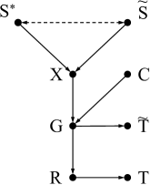
Figure 3: Graphical representation of the SCM.

SCM.

We adopt SCM to conduct causal modeling. SCM [30] is a framework utilized to describe the manner in which nature assigns values to variables of interest. Formally, an SCM consists of variables and the relationships between them. Each SCM can be represented as a graphical model consisting of a set of nodes representing the variables, and a set of edges between the nodes representing the relationships.

We formalize the candidate problem by using an SCM illustrated in Figure 3. The validity of this SCM is proved based on the Inductive Causation (IC) algorithm [32], as demonstrated in Appendix A.1. Among the SCM, the variables $S^{*}$ and $\widetilde{S}$ represent the graph causal factors, which hold a direct causal relationship with the graph data. $\widetilde{S}$ denotes the accessible graph causal factors that can be discerned with the available expertise logic. $S^{*}$ denotes the rest graph causal factors. The variable $X$ represents the embodiments of $S^{*}$ and $\widetilde{S}$ within the graph data. For ease of understanding such concepts, we establish an intuitive illustration: $\widetilde{S}$ can present the topology structure of a graph, $S^{*}$ are the other properties of the graph. If the value of $\widetilde{S}$ is "cyclic", then its embodiment, which is contained in $X$, will take a cyclic structure. Please note that this is merely a simplified example for illustrative purposes, and obtaining all the relevant expertise logic for the whole structure of a graph in practical tasks is not feasible. $C$ represents any confounding factors present within the data, $G$ represents the graph data itself, and $R$ represents the learned representation of the graph data. $\widetilde{T}$ and $T$ are the outputs of the high-level causal model and the GNN. The links in Figure 3 are as follows:

• $S^{*}\to X,\widetilde{S}\to X.$ $X$ denotes the embodiment of $S^{*}$ and $\widetilde{S}$ within the graph data.

• $X\to G\leftarrow C.$ The graph data $G$ consists of two parts: X and confounder $C$.

• $G\to R.$ A GNN encoder encodes $G$ into representation $R$ that consists of the node representations of different layers and the graph representation.

• $S^{*}\dashedleftarrow\dashedrightarrow\widetilde{S}.$ The bidirectional arrow with a dashed line indicates that the causal relationship between the two cannot be confirmed.

• $G\to\widetilde{T},R\to T.$ $\widetilde{T}$ and $T$ are variables that calculated based on $G$ and $R$.

4.2 Analysis based on the causal models

Based on SCM in Figure 3, we provide theoretical proof to support the intuition that acquiring prior knowledge about graph causal factors is beneficial for enhancing a model’s performance. To achieve such a goal, We propose the following theorem.

Theorem 4.1.

For a graph representation learning process with a causal structure represented by the SCM in Figure 3, increasing the mutual information $I(R;\widetilde{S})$ between $R$ and $\widetilde{S}$ can decrease the upper bound of the mutual information $I(R;C)$ between $R$ and $C$. Formally:

$$I(R;C)\leq 1-I(R;\widetilde{S}).$$ (9)

The proof of Theorem 4.1 can be found in Appendix A.2. Theorem 4.1 establishes a direct relationship between a model’s understanding of graph causal factors and the reduction of confounding influence. As the model gains a deeper understanding of graph causal factors, the confounding influence diminishes. Next, we prove the validity of the training objective proposed by Equation 2.

Theorem 4.2.

For a certain graph learning process with a causal structure represented by the SCM in Figure 3, $\widetilde{T}\sim p(t),T\sim q(t),t\in\mathcal{T}$, if the high-level causal models $r(\cdot)$ is effective enough such that $I(\widetilde{T},\widetilde{S})=I(G,\widetilde{S})$, then $I(R,\widetilde{S})$ is maximized if $p(t|\widetilde{s})=q(t|\widetilde{s})$.

The proof of Theorem 4.2 can be found in Appendix A.3. According to Theorem 4.2, if Equation 2 holds, $I(R,\widetilde{S})$ will be maximized, which indicates that the model has learned the maximum amount of knowledge about $\widetilde{S}$. With Theorem 4.2, we present a corollary to substantiate the validity of $\mathcal{L}_{c}$.

Corollary 4.3.

For a specific graph dataset $G$, if the training samples in $G$ sufficiently cover all embodiments corresponding to $\widetilde{S}$, and the $\mathcal{L}_{c}$ which is defined by Equation 4 reaches zero, then the maximized value of $I(R,\widetilde{S})$ stated in Theorem 4.2 can be achieved.

The proof is presented in Appendix A.4.

5 Experiments

In this section, we carry out multiple experiments aimed at addressing the research questions:

• RQ1: How effective is CLGL in learning expertise logic? Furthermore, Can such expertise logic be applied to various datasets?

• RQ2: How does CLGL differ from conventional methods? How does the knowledge of expertise logic specifically assist in such a training process?

5.1 Settings

Datasets.

For experiments, we employed two distinct types of datasets, one comprising comprehensive topological structure information and the other containing rich node attribution information.

For the topological structure information abundant datasets, we developed a high-level causal model based on general topology prior knowledge and trained it on multiple datasets, including:1) Spurious-Motif, a synthetic Out Of Distribution (OOD) dataset [34] based on the data generation method of [37]; 2) Motif-Variant, also a synthetic OOD dataset that is created by ourselves using the data generation method following [37], while the internal topological structure is different from the previous dataset. 3) The In-Distribution (ID) version of these datasets. To guarantee the fairness and efficacy of our experiments, the high-level causal model we devised did not integrate any information directly related to downstream tasks, but rather comprised only generic topological structure knowledge. Additionally, we confirmed our method’s universality through validation on multiple datasets with the same high-level causal model.

Table 1: Performance of classification accuracy in Spurious-Motif. Spurious-Motif (ID) denotes the ID version dataset. Bias represents the degree of distribution shift between the training set and the test set. Some of the results are cited from [34]. The best records are highlighted in bold.

Method	Spurious-Motif				Spurious-Motif
	Balanced	bias = 0.5	bias = 0.7	bias = 0.9	(ID)
ERM	42.99$\pm$1.93	39.69$\pm$1.73	38.93$\pm$1.74	33.61$\pm$1.02	92.91$\pm$1.98
GAT [31]	43.07$\pm$2.55	39.42$\pm$1.50	37.41$\pm$0.86	33.46$\pm$0.43	91.31$\pm$2.28
Top-k Pool [9]	43.43$\pm$8.79	41.21$\pm$7.05	40.27$\pm$7.12	33.60$\pm$0.91	90.83$\pm$3.04
GSN [3]	43.18$\pm$5.65	34.67$\pm$1.21	34.03$\pm$1.69	32.60$\pm$1.75	92.81$\pm$1.10
Group DRO [29]	41.51$\pm$1.11	39.38$\pm$0.93	39.32$\pm$2.23	33.90$\pm$0.52	92.18$\pm$1.12
IRM [1]	42.26$\pm$2.69	41.30$\pm$1.28	40.16$\pm$1.74	35.12$\pm$2.71	91.12$\pm$1.56
V-REx [15]	42.83$\pm$1.59	39.43$\pm$2.69	39.08$\pm$1.56	34.81$\pm$2.04	91.08$\pm$1.85
DIR [34]	42.53$\pm$3.38	41.45$\pm$2.12	41.03$\pm$1.53	39.20$\pm$1.94	93.02$\pm$1.89
CLGL-D	42.83$\pm$2.33	40.13$\pm$1.94	39.08$\pm$1.68	34.11$\pm$2.02	91.69$\pm$1.30
CLGL-A	47.08$\pm$1.56	43.03$\pm$1.90	41.15$\pm$1.54	40.13$\pm$1.89	94.03$\pm$1.28
CLGL	52.18$\pm$2.35	50.11$\pm$1.92	49.02$\pm$1.79	43.31$\pm$2.07	96.53$\pm$1.28

Table 2: Performance of classification accuracy in Motif-Variant. Motif-Variant (ID) denotes the ID version dataset. Bias represents the degree of distribution change between the training set and the test set. The best records are highlighted in bold.

Method	Motif-Variant				Motif-Variant
	Balanced	bias = 0.5	bias = 0.7	bias = 0.9	(ID)
ERM	48.18$\pm$3.46	46.38$\pm$2.52	45.78$\pm$2.81	42.31$\pm$2.13	94.78$\pm$1.07
GAT [31]	49.13$\pm$2.96	47.78$\pm$2.12	45.63$\pm$1.93	41.48$\pm$0.85	93.32$\pm$2.60
Top-k Pool [9]	48.56$\pm$7.10	46.08$\pm$7.93	44.37$\pm$8.07	42.10$\pm$6.13	93.17$\pm$3.21
GSN [3]	47.05$\pm$6.03	44.08$\pm$2.32	43.15$\pm$1.68	40.19$\pm$1.93	93.90$\pm$2.11
Group DRO [29]	44.03$\pm$1.38	42.06$\pm$1.21	41.15$\pm$1.56	39.90$\pm$1.02	92.54$\pm$1.31
IRM [1]	48.13$\pm$2.86	44.30$\pm$1.49	42.01$\pm$2.03	40.18$\pm$2.33	93.17$\pm$1.21
V-REx [15]	49.76$\pm$1.68	46.83$\pm$2.36	43.12$\pm$1.50	42.37$\pm$1.99	93.13$\pm$1.25
DIR [34]	49.66$\pm$2.85	47.76$\pm$2.73	44.80$\pm$1.32	42.90$\pm$1.68	94.46$\pm$1.57
CLGL-D	48.01$\pm$1.87	47.05$\pm$1.62	45.37$\pm$1.49	42.11$\pm$1.83	92.01$\pm$0.86
CLGL-A	48.96$\pm$1.73	48.60$\pm$1.43	46.23$\pm$1.43	45.80$\pm$1.87	93.56$\pm$0.99
CLGL	55.36$\pm$2.38	53.00$\pm$2.10	49.84$\pm$2.32	47.96$\pm$1.87	97.57$\pm$0.92

Table 3: Performance of classification accuracy in Graph-SST5 and Graph-Twitter. Graph-SST5 (OOD) and Graph-Twitter (OOD) denote the OOD version datasets. The best records are highlighted in bold.

Method	Graph-SST5	Graph-SST5	Graph-Twitter	Graph-Twitter
		(OOD)		(OOD)
ERM	49.02$\pm$0.82	39.39$\pm$0.66	65.46$\pm$1.01	63.04$\pm$1.46
GAT [31]	48.51$\pm$1.86	37.58$\pm$1.67	63.57$\pm$0.95	62.38$\pm$0.98
Top-k Pool [9]	49.72$\pm$1.42	36.26$\pm$1.86	63.41$\pm$1.95	62.95$\pm$1.09
GSN [3]	48.64$\pm$1.60	38.78$\pm$1.84	63.18$\pm$1.89	63.07$\pm$1.18
Group DRO [29]	47.44$\pm$1.12	37.78$\pm$1.12	62.23$\pm$1.43	61.90$\pm$1.03
IRM [1]	48.08$\pm$1.30	38.68$\pm$1.62	64.11$\pm$1.58	62.27$\pm$1.55
V-REx [15]	48.55$\pm$1.10	37.10$\pm$1.18	64.84$\pm$1.46	63.42$\pm$1.06
DIR [34]	49.16$\pm$1.31	38.67$\pm$1.38	65.14$\pm$1.37	63.49$\pm$1.36
CLGL-D	48.93$\pm$0.76	38.85$\pm$1.53	64.79$\pm$1.05	62.18$\pm$0.83
CLGL-A	49.63$\pm$0.89	39.00$\pm$1.25	65.32$\pm$0.93	61.98$\pm$0.96
CLGL	50.38$\pm$0.87	42.13$\pm$1.50	66.68$\pm$0.81	63.98$\pm$1.20

For the node attribution information abundant datasets, we developed another high-level causal model. We also ensure that the model contains only generic knowledge that does not directly relate to downstream tasks, and conduct experiments with the same high-level causal model on multiple real-world datasets, including Graph-SST5 [39], Graph-Twitter [39], and their OOD versions. The details of the high-level causal model and the datasets can be found in Appendix C and B.1.

Baselines.

We compare our method with Empirical Risk Minimization (ERM) and various causality-enhanced methods that can be divided into two groups: 1) the interpretable baselines, including GAT ,Top-k Pool and GSN, 2) the robust learning baselines, including Group DRO, IRM, V-REx and DIR. For a fair comparison, we follow the experimental principles of [34] and adopt the same training setting for all models, which is described in Appendix B in detail. For each task, we report the mean performance ± standard deviation over five runs. For further demonstration of the universality of our proposed method, we also construct the CLGL-D model. CLGL-D directly employs the output of the higher-order causal model $r(\cdot)$ as labels for training, along with the existing labels within the dataset. Consequently, we can assess whether the output of $r(\cdot)$ contains information directly relevant to downstream tasks that may aid the training procedure. Furthermore, to showcase the benefits of our proposed enhancement with interchange interventions, we develop the CLGL-A model to conduct corresponding ablation studies, which removes the enhancement with interchange interventions.

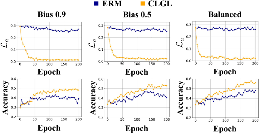
(a) Accuracy and loss obtained over 200 epochs on multiple Motif-Variant datasets with distinct biases.

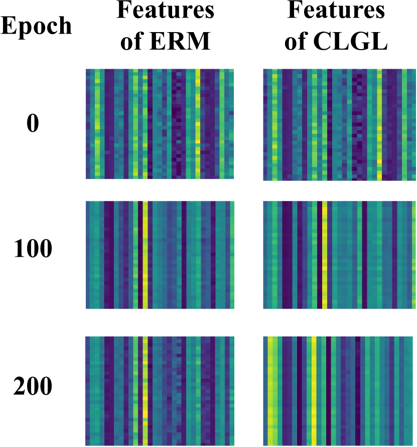
(b) Visualized features

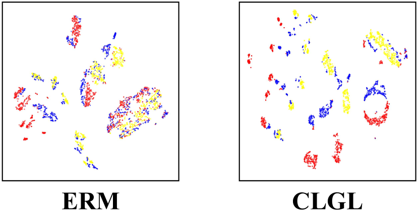
(c) Features after dimensionality reduction using t-SNE [21]

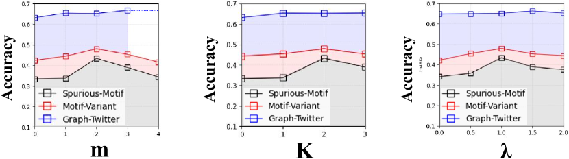
(d) Parameter experiments conducted on different datasets

Figure 4: Results of further experiments.

5.2 Comparison with State-of-the-art Methods (RQ1)

The results are reported in Table 1, 2, and 3. We observe from the tables and find that our method outperforms all baselines on all downstream tasks by large margins. Another observable phenomenon is that CLGL significantly outperforms CLGL-D. Since the expertise logic we introduced represents universal graph knowledge not specific to any downstream task, directly utilizing this universal knowledge cannot enhance the model’s performance on downstream tasks. However, CLGL surpasses state-of-the-art performance, indicating that using graph neural networks to learn universal expertise logic can help them acquire logical inductive capabilities, enabling them to better extract discriminative information from graph data. Furthermore, it is observable that CLGL outperforms CLGL-A, which verifies the necessity of our proposed enhancement with interchange interventions.

5.3 In-Depth Study (RQ2)

To understand how our model changes during training, we tracked accuracy and $\mathcal{L}_{a}$ loss across 200 epochs on multiple Motif-Variant datasets with different biases. $\mathcal{L}_{a}$ for ERM was calculated similarly to CLGL but without backpropagation. Results in Figure 4(a) show that CLGL’s $\mathcal{L}_{a}$ decreases quickly and stays consistently low, while its performance keeps improving even after multiple epochs. This suggests that CLGL can effectively learn and maintain the correct logic without degradation. Different biases had little impact on $\mathcal{L}_{a}$, indicating that the expertise logic isn’t closely tied to downstream tasks. Therefore, its learning efficiency isn’t affected by dataset variations.

Figure 4(b) shows visualized output features of our model. Each horizontal line in each block represents the model’s representation of graph data, with the vertical axis representing different samples from the same class. Consistent vertical lines indicate a more consistent representation of causal information within the graph data across samples. CLGL produces more consistent representations at the 100th and 200th epochs compared to ERM, indicating better expertise logic learning. Additionally, there are significant changes in CLGL’s representations between the 100th and 200th epochs, indicating the model is continually learning. Figure 4(c) displays different methods’ feature representations of test samples at the 200th epoch, revealing that CLGL offers a more refined and accurate representation.

Figure 4(d) demonstrates the impact of different hyperparameters on the model. The experimental results regarding $m$ and $K$ substantiate that extracting representations in the intermediate layers for causal knowledge learning, while simultaneously employing multiple interchange interventions, effectively enhances the model’s performance. And, $\lambda$ can aid in striking a balance between causal learning and dataset training. These results validate the necessity of our proposed structures.

6 Conclusions

Through empirical observations of motivating experiments, we find that GNNs tend to learn human expertise during training, and introducing expertise logic into graph representation learning improves the model performance. Hence, we propose CLGL, a method that guides the model to learn expertise logic. The validity and effectiveness of our design are supported by theoretical analysis, highlighting its key strengths and justification. Empirical comparisons demonstrate the significant performance improvements achieved by our approach.

Limitations. Our work is based on experimental observations to propose a novel research question and provide a solution. However, there is room for improvement in the optimization of the specific training process. Furthermore, the acquisition of expertise logic, which we utilized, actually requires extensive analytical work. Therefore, we will consider developing methods to automatically extract expertise logic from datasets in the future.

Appendix A Proofs

A.1 A Validity Justification For The SCM In Figure 3

To establish the validity of the proposed SCM in Figure 3, we employ the IC algorithm [30] to construct the SCM from scratch and provide the detailed construction process. IC algorithm is a method for identifying causal relationships from the ob +served data. Please refer to Chapter 2 of [30] for the details of the IC algorithm.

The input of the IC algorithm is a set of variables and their distributions. The output is a pattern that represents the underlining causal relationships, which can be a structural causal model. The IC algorithm can be divided into three steps:

Step 1.

For each pair of variables $a$ and $b$ in $V$, the IC algorithm searches for a set $S_{ab}$ s.t. the conditional independence relationship $(a\upmodels b|S_{ab})$ holds. In other words, $a$ and $b$ should be independent given $S_{ab}$. The algorithm constructs an undirected graph $G$ with vertices corresponding to variables in $V$. A pair of vertices $a$ and $b$ are connected with an undirected edge in $G$ if and only if no set $S_{ab}$ can be found that satisfies the conditional independence relationship $(a\upmodels b|S_{ab})$.

Step 2.

For each pair of non-adjacent variables $a$ and $b$ that share a common neighbor $c$, check the existence of $c\in S_{ab}$. If such a $c$ exists, proceed to the next pair; if not, add directed edges from $a$ to $c$ and from $b$ to $c$.

Step 3.

In the partially directed graph results, orient as many of the undirected edges as possible subject to the following two conditions: (i) any alternative orientation of an undirected edge would result in a new y-structure, and (ii) any alternative orientation of an undirected edge would result in a directed cycle.

Accordingly, we employ IC algorithm to provide a step-by-step procedure for constructing our structural causal model.

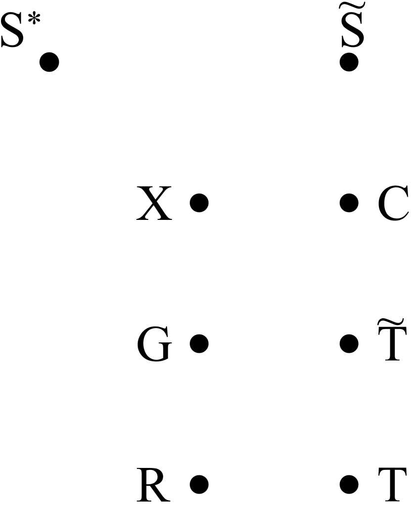
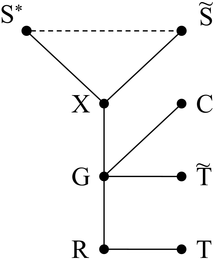
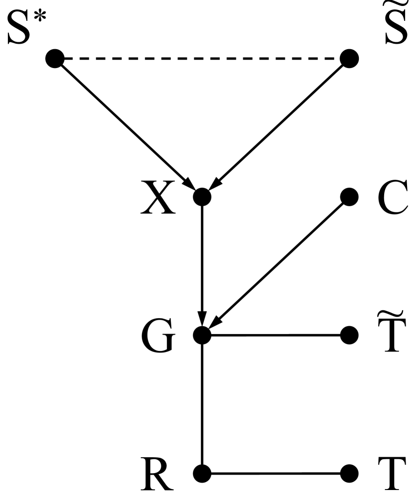
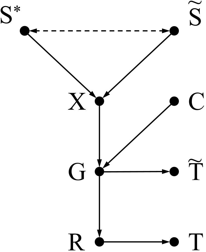
Figure 5: Visualization of the reasoning process using IC algorithm.

As for step 1, we first represent all variables as nodes in Figure 5. For each node, we traverse all other nodes to determine whether to establish a connection. Accordingly, $R$ represents the model’s representation of $G$. Since any other variable can only affect $R$ through $G$, $R$ is conditionally independent of all other variables given $G$. Therefore, $R$ is only connected to $G$. $G$ represents the graph data, which is composed of $X$ and $C$. There is no other variable that can block the relationship between $G$ and $X$, or $G$ and $C$. Therefore, $G$ is connected to both $X$ and $C$. As $X$ blocks the path from $S^{*}$ and $\widetilde{S}$ to $G$, the corresponding connections do not exist. We define $C$ as a confounder in the graph data, which has no causal relationship with other variables. Therefore, an empty set can make $C$ independent of other variables, except for $G$.

As $\widetilde{S}$ and $S^{*}$ are all graph causal factors, each of them is correlated with $X$. Their connections cannot be blocked by any set of variables, and thus we connect all these nodes with $X$. The relationship between $S^{*}$ and $\widetilde{S}$ can not be figured out, therefore we adopt a dashed line to link them. The result is demonstrated in Figure 5.

We then move on to step 2. Similar to step 1, we process with the traversal analysis starting from $R$. For $R$, since $G\in S_{RG}$ and $G\in S_{RX}$, no edges related to $R$ can be directed. Then, as $S_{XC}=\emptyset$, $X\notin S_{XC}$, we direct edge $X$ to $G$ and $C$ to $G$. As $S^{*}$ and $\widetilde{S}$ is the cause of $X$ by definition, therefore we direct edge $S^{*}$ to $X$ and $\widetilde{S}$ to $X$.

In Step 3, we adopted the rule 1 from [33] for systematizing this step, which states that if $a\to b$ and $a$ and $c$ are not adjacent, then $b\to c$ should be set as the orientation for $b-c$. Based on this, we established the following orientations: $G\to\widetilde{T},G\to R$. Then, according to the same rule, $R\to T$ should also be set. As for the remaining edge $(\widetilde{S},S^{*})$, since we cannot determine its direction, we represent this edge with a bidirectional dashed line, indicating its directionality is uncertain. The final result is illustrated in Figure 5, which is identical to the SCM in Figure 3.

A.2 Proof of Theorem 4.1

To prove the theorem, we follow [25] and suppose the proposed SCM possesses Markov property. Therefore, according to the SCM in Figure 3, $C$ and $R$ are conditionally independent given $G$, as $G$ blocks any path between $C$ and $R$. Therefore, we could apply the Data Processing Inequality [5] on the path $C\to G\to R$. Formally, we have:

$$I(G;C)\geq I(R;C).$$ (10)

According to the Chain Rule for Information [5], we also have:

$$I(X,C;G)=I(X;G|C)+I(C;G).$$ (11)

As $X$ and $C$ are independent, we have:

$$I(X,C;G)=I(X;G)+I(C;G).$$ (12)

Therefore:

$$I(C;G)=I(X,C;G)-I(X;G).$$ (13)

As $G$ is the graph data that consist of $X$ and $C$, we have:

$$I(X,C;G)=1.$$ (14)

Then:

$$I(C;G)=1-I(X;G).$$ (15)

Therefore:

$$1-I(X;G)\geq I(R;C).$$ (16)

According to the SCM in Figure 3, $\widetilde{S}$ and $R$ are conditionally independent given $G$, we have:

$$I(\widetilde{S};G)\geq I(\widetilde{S};R).$$ (17)

Also:

$$I(\widetilde{S},X;G)=I(\widetilde{S};G)+I(X;G|\widetilde{S})$$ (18)

and

$$I(\widetilde{S},X;G)=I(X;G)+I(\widetilde{S};G|X)$$ (19)

holds. $\widetilde{S}$ and $G$ is independent given $X$, therefore:

$$I(\widetilde{S};G|X)=0.$$ (20)

Thus:

$$I(\widetilde{S},X;G)=I(\widetilde{S};G)+I(X;G|\widetilde{S})=I(X;G).$$ (21)

As $I(X;G|\widetilde{S})\geq 0$:

$$I(\widetilde{S};G)\leq I(X;G).$$ (22)

Based on Inequality 17 and 22, we have:

$$I(\widetilde{S};R)\leq I(X;G).$$ (23)

Substituting Inequality 23 into Inequality 16, we can obtain:

$$I(R;C)\leq 1-I(\widetilde{S};R).$$ (24)

The theorem is proved.

A.3 Proof of Theorem 4.2

We begin with calculating the boundaries of $I(R,\widetilde{S})$. According to the SCM in Figure 3, $\widetilde{S}$ and $G$ are conditionally independent given $X$, as $X$ block any path between $\widetilde{S}$ and $G$. Therefore, we could apply the Data Processing Inequality [5] on the path $\widetilde{S}\to X\to G$. Formally, we have:

$$I(\widetilde{S};X)\geq I(\widetilde{S};G).$$ (25)

Likewise, we have:

$$I(\widetilde{S};G)\geq I(\widetilde{S};R),$$ (26)

and:

$$I(\widetilde{S};R)\geq I(\widetilde{S};T).$$ (27)

According to the assumptions:

$$I(\widetilde{T};\widetilde{S})=I(G;\widetilde{S}),$$ (28)

we have:

$$I(\widetilde{S};\widetilde{T})\geq I(\widetilde{S};R)\geq I(\widetilde{S};T).$$ (29)

So far, we can acquire the upper and lower bounds of $I(\widetilde{S};R)$. Moreover, since the data set and the expert system are determined in advance in the learning task, the only thing that can be changed for this system is the parameters of the neural network model. Therefore, the upper bound $I(\widetilde{S};\widetilde{T})$ holds a fixed value. If we can make the lower bound $I(\widetilde{S};T)$ equal to the upper bound $I(\widetilde{S};\widetilde{T})$, then we have $I(\widetilde{S};R)$ reached the maximum. Next, we will proof if $p(t|\widetilde{s})=q(t|\widetilde{s})$, then $I(\widetilde{S};\widetilde{T})=I(\widetilde{S};T)$.

When $p(t|\widetilde{s})=q(t|\widetilde{s})$, then:

$$H(T|\widetilde{S}) =-\sum_{\widetilde{s}\in\mathcal{\widetilde{S}}}p_{\widetilde{S}}(\widetilde{s})\sum_{t\in\mathcal{T}}p(t|\widetilde{s})log\Big{(}p(t|\widetilde{s})\Big{)}$$

$$=-\sum_{\widetilde{s}\in\mathcal{\widetilde{S}}}p_{\widetilde{S}}(\widetilde{s})\sum_{t\in\mathcal{T}}q(t|\widetilde{s})log\Big{(}q(t|\widetilde{s})\Big{)}$$

$$=H(\widetilde{T}|\widetilde{S}),$$ (30)

where $\widetilde{S}\sim p_{\widetilde{S}}(\widetilde{s}),\widetilde{s}\in\mathcal{\widetilde{S}}$.

We also have:

$$H(T) =-\sum_{t\in\mathcal{T}}p(t)log\Big{(}p(t)\Big{)}$$

$$=-\sum_{t\in\mathcal{T}}\sum_{\widetilde{s}\in\mathcal{\widetilde{S}}}p_{\widetilde{S}}(\widetilde{s})p(t|\widetilde{s})log\Big{(}\sum_{\widetilde{s}\in\mathcal{\widetilde{S}}}p_{\widetilde{S}}(\widetilde{s})p(t|\widetilde{s})\Big{)}$$

$$=-\sum_{t\in\mathcal{T}}\sum_{\widetilde{s}\in\mathcal{\widetilde{S}}}p_{\widetilde{S}}(\widetilde{s})q(t|\widetilde{s})log\Big{(}\sum_{\widetilde{s}\in\mathcal{\widetilde{S}}}p_{\widetilde{S}}(\widetilde{s})q(t|\widetilde{s})\Big{)}$$

$$=-\sum_{t\in\mathcal{T}}q(t)log\Big{(}q(t)\Big{)}$$

$$=H(\widetilde{T})$$ (31)

According to the definition of mutual information [5], we have:

$$I(\widetilde{S};\widetilde{T})=H(\widetilde{T})-H(\widetilde{T}|\widetilde{S}),$$

$$I(T;\widetilde{S})=H(T)-H(T|\widetilde{S}).$$ (32)

Based on equation 30, 31 and 32, we have:

$$I(\widetilde{S};\widetilde{T})=I(\widetilde{S};T).$$ (33)

Based on the discussions above, $I(\widetilde{S};R)$ reached the maximum. The theorem is proved.

A.4 Proof of Corollary 4.3

As in Equation 2, for each graph $G_{i}$, $\widetilde{S}$ holds a fixed value $\widetilde{s}_{i}$. Therefore, we have:

$$p_{i}(t)=p_{i}(t|\widetilde{s}_{i})=p_{i}(t|\widetilde{s}),$$ (34)

and

$$\hat{q}_{i}(t)=\hat{q}_{i}(t|\widetilde{s}_{i})=\hat{q}_{i}(t|\widetilde{s}).$$ (35)

Therefore, we have:

$$\mathcal{L}_{c}=\sum_{i}^{N}KL\Big{(}p_{i}(t|\widetilde{s})||\hat{q}_{i}(t|\widetilde{s})\Big{)}=\sum_{i}^{N}KL\Big{(}p_{i}(t)||\hat{q}_{i}(t)\Big{)}$$ (36)

As $r^{P}(r^{E}(G_{i}))$ can predict $p_{i}(t)$. $f^{P}(f^{E}(G_{i}))$ output a estimation $\hat{q}_{i}(t)$ of ${q}_{i}(t)$. Therefore:

$$\mathcal{L}_{c}=\sum_{i}^{N}KL\Big{(}p_{i}(t)||\hat{q}_{i}(t)\Big{)}=\sum_{i=1}^{N}\mathcal{D}_{KL}\Big{(}r^{P}(r^{E}(G_{i})),f^{P}(f^{E}(G_{i}))\Big{)}$$ (37)

Then, if:

$$\mathcal{L}_{c}=\sum_{i=1}^{N}\mathcal{D}_{KL}\Big{(}r^{P}(r^{E}(G_{i})),f^{P}(f^{E}(G_{i}))\Big{)}=0,$$ (38)

we have:

$$\sum_{i}^{N}KL\Big{(}p_{i}(t)||\hat{q}_{i}(t)\Big{)}=\sum_{i}^{N}KL\Big{(}p_{i}(t|\widetilde{s})||\hat{q}_{i}(t|\widetilde{s})\Big{)}=0.$$ (39)

Further more, the training samples in $G$ sufficiently cover all embodiments corresponding to $\widetilde{S}$, we have:

$$KL\Big{(}p(t|\widetilde{s})||q(t|\widetilde{s})\Big{)}=0.$$ (40)

Then $p(t|\widetilde{s})$ equals $q(t|\widetilde{s})$, according to Theorem 4.2, $I(R;\widetilde{S})$ reaches maximization. The Corollary is proved.

Appendix B Experiment Setting Details.

In this section, we give a detailed description of our experiment settings.

Table 4: Summary of datasets.

Name	Graphs#	Average Nodes#	Classes#	Task Type	Metric
Spurious-Motif	18,000	46.6	3	Classification	ACC
Motif-Variant	18,000	48.9	3	Classification	ACC
Graph-SST5	11,550	21.1	5	Classification	ACC
Graph-Twitter	6,940	19.8	3	Classification	ACC

Table 5: Summary of the backbones used in each dataset.

Dataset	Backbone	GNN structure	Global Pool
Spurious-Motif	Local Extremum GNN	[4,32,32,32]	global mean pool
Motif-Variant	Local Extremum GNN	[4,32,32,32]	global mean pool
Graph-SST5	ARMA	[768,128,128]	global mean pool
Graph-Twitter	ARMA	[768,128,128]	global mean pool

B.1 Datasets

We evaluate our method on four different datasets, and the ID/OOD version of these datasets. The datasets are built upon manually constructed data and sentiment graph data. We summarize the datasets we used in Table 4. Furthermore, we demonstrate the backbone GNN we adopt for each dataset in Table 5. The GNNs we utilized included Local Extremum GNN [28], ARMA [23].

Spurious-Motif. Spurious-Motif is an OOD synthetic dataset proposed by [37]. We adopt a reimplemented version created by [34]. The dataset involves 18,000 graphs, each one of them consisting of two subgraphs: motif and confounder. The motif consists of ground truth data with fixed structures and is causally related to the ground truth label. Confounder, on the other hand, has no causal relationship with the labels. Spurious-Motif possessed three types of motifs and confounders. In the training set, confounders are stitched into the graph data with certain biases. For example, a bias of 0.9 means that for each class, 90$\%$ of motifs and confounders that are stitched together belong to the same class. The motifs and confounders in the test set are appended randomly. Therefore, the greater the bias, the harder it is for the model to distinguish between causal information and confounders. Additionally, the test graph data includes large subgraphs to make the learning task harder.

Motif-Variant. As the causal information in Spurious-Motif consists of motifs with fixed structures, we modify the dataset to have more varied data. Instead of fixed structures, we adopt different kinds of motifs and allow some shape changes on them. Based on such changes, we are able to create a larger gap between the training and the test set.

Graph-SST5. Graph-SST5 dataset [39] is an ID sentiment graph dataset that builds upon the Rotten Tomatoes comments.

Graph-Twitter. Graph-Twitter dataset [39] is also a sentiment graph dataset. However, its data comes from the comments on Twitter.

Spurious-Motif (ID). The ID version of Spurious-Motif, which removes the bias and the large subgraphs in test data.

Motif-Variant (ID). The ID version of Motif-Variant, following the same pattern as Spurious-Motif (ID).

Graph-SST5 (OOD). The OOD version of Graph-SST5. We follow [34] to split the graph samples into different sets according to their average node degree.

Graph-Twitter (OOD). The OOD version of Graph-Twitter, in which we adopt the same modification pattern as Graph-SST5 (OOD).

B.2 Environments and Optimization Method

All our experiments are performed on a workstation equipped with two Quadro RTX 5000 GPUs (16 GB), an Intel Xeon E5-1650 CPU, 128GB RAM and Ubuntu 20.04 operating system. We employ the Adam optimizer for optimization. We set the maximum training epochs to 400 for all tasks. For backpropagation, we optimize Graph-SST2 and Graph-Twitter using stochastic gradient descent (SGD), while utilizing gradient descent (GD) on Spurious-Motif and Motif-Variant.

B.3 Hyperparameters

As for the hyperparameters, we set $m$ to 2 for the Spurious-Motif and Motif-Variant datasets, and 3 for the Graph-SST5 and Graph-Twitter datasets. We set $\lambda$ to 1 for the Spurious-Motif and Motif-Variant datasets and 1.5 for the Graph-SST5 and Graph-Twitter datasets. We set $K$ as 3 for all datasets. We set the learning rate as 0.001 for Spurious-Motif and Motif-Variant and 0.0002 for others. We train our model for 200 epochs, then stop training early if there is no performance improvement on the validation set for five epochs. We choose the model with the best validation performance as the final result. The maximum number of training epochs is set to 400 for all datasets. The training batch size is set as 32 for all datasets. The structure of GNN adopted for different datasets is shown in the table 5.

Appendix C Implementation Details

To guide GNNs to learn expertise logic, we build multiple higher-order causal models corresponding to different kinds of expert logic. In this part, we will describe the detailed implementations of these models, along with other detailed implementations of CLGL.

C.1 Implentation of $r^{E}(\cdot)$

$r^{E}(\cdot)$ concerning structure information

The expertise logic we employ is the "structural morphology of connections between subgraphs." As datasets rich in structural information often consist of multiple substructures with distinct features, the information regarding the structural morphology at the connections between these substructures becomes an expertise logic that can help guide the neural network learning more knowledge. Specifically, to enable the recognition of connection points by $r^{E}(\cdot)$, we first preprocess the graph data used for training and identify and label the connection points using topological structure matching techniques. For ease of training, we only label one connection point per graph sample, and this label also guides the training of $f^{P}(\cdot)$. Due to the reuse of training data, this representation will be precomputed in advance.

Due to our assumption of $I(\widetilde{T};\widetilde{S})=I(G;\widetilde{S})$ in Theorem 4.2, we hereby provide an explanation for why the designed $r^{E}(\cdot)$ adheres to this assumption. We can assert that $\widetilde{S}$ in our discussion represents the analyzable and representable aspects of $r^{E}(\cdot)$ based on G. Thus, even if $G$ may contain information beyond $I(G;\widetilde{S})$, we can exclude it from the scope of $\widetilde{S}$.

$r^{E}(\cdot)$ concerning node attribution

We have designed a second type of $r^{E}(\cdot)$ based on node attribute-related information. Since our target dataset is related to natural language, we utilize the concept of conjunctions, specifically the conjunction "but" and its representation of contrast relationships, as the expertise logic for designing $r^{E}(\cdot)$. Specifically, we preprocess the graph data used for training and identify the nodes corresponding to "but" and the nodes representing the respective sentences in which they appear. $r^{E}(\cdot)$ then outputs the degree of semantic contrast between the text preceding and following "but."

C.2 Implentation of $r^{I}(\cdot)$

In practice, due to the difficulty of finely modeling the composition of graph data in multiple cases, the expertise logic we can obtain contains rather generic knowledge. In such situations, the space of possible values for the graph causal factor may be small. Training an $r^{E}(\cdot)$ under such conditions would be ineffective. Therefore, we perform interchange intervention operations. Based on such operations, $r^{I}(\cdot)$ will introduce other information beyond embodiment to change its value. As demonstrated in Equation 5, $r^{I}(\cdot)$ generates different weights based on the type of interchange intervention. The specific type of interchange intervention performed directly determines the weights that $h(\cdot)$ outputs. Specifically, different interchange interventions can induce changes in the learned representation of the embodiment. We assess the magnitude of these changes and subsequently evaluate the probability that the post-intervention embodiment belongs to the same category as the pre-intervention embodiment. Based on this assessment, we generate the weights accordingly.

C.3 Implentation of $r^{P}(\cdot)$

$r^{P}(\cdot)$ predicts the probabilities of different values for the graph causal factor based on the output of $r^{E}(\cdot)$. The predicted values are determined using a predefined formula, which would project the outputs of $r^{E}(\cdot)$ into a vector that represents the probability density function. Such a vector will then be used to calculate the KL divergence.

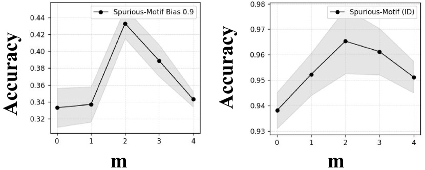
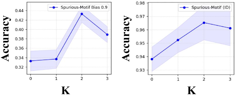
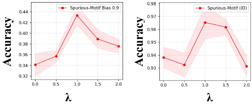
Figure 6: Performance of CLGL on Spurious-Motif dataset with different hyperparameter values. The translucent region represents the confidence interval of the results.

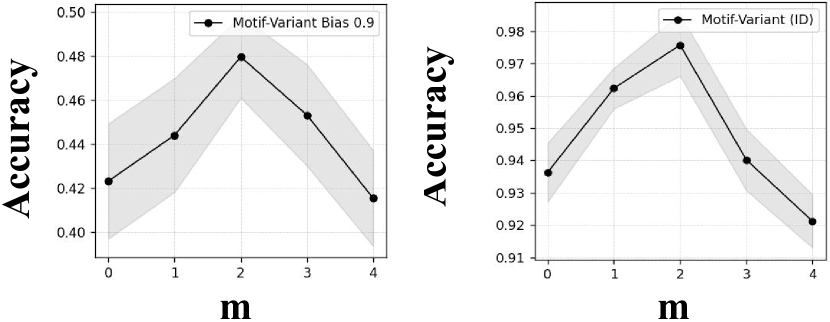
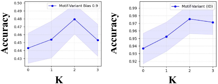
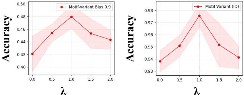
Figure 7: Performance of CLGL on Motif-variant dataset with different hyperparameter values. The translucent region represents the confidence interval of the results.

C.4 Implentation of $f^{P}(\cdot)$

Based on the previously determined labels, $f^{P}(\cdot)$ takes the labeled nodes as input, along with the number of neural network layers determined by hyperparameters. Through pooling and multi-Layer perceptron, it ultimately outputs distribution predictions. The prediction is a vector of dimensionality equal to the number of categories, and it has undergone normalization.

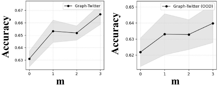
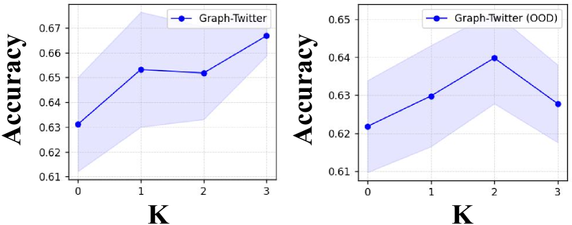
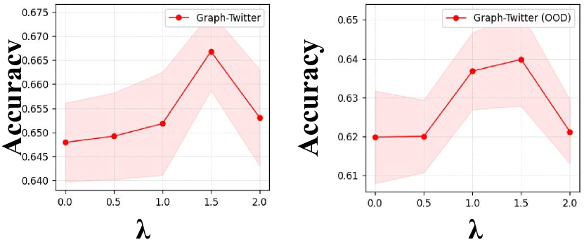
Figure 8: Performance of CLGL on Graph-Twitter dataset with different hyperparameter values. The translucent region represents the confidence interval of the results.

Appendix D Additional Hyperparameter Experiments

This section presents further parameter experiments. The experimental results are shown in Figures 6, 7, 8 and 9. From the figures, we can observe that while the optimal values of certain parameters vary across different versions of the datasets, we still chose to use the same parameters to avoid introducing additional prior knowledge.

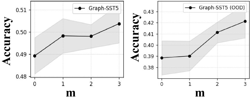
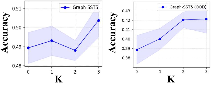
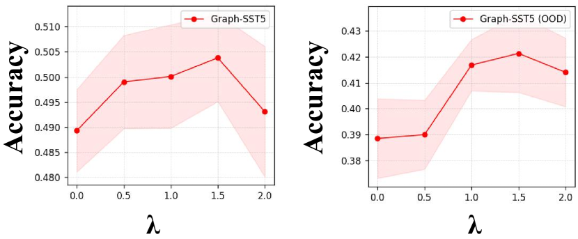
Figure 9: Performance of CLGL on Graph-SST5 dataset with different hyperparameter values. The translucent region represents the confidence interval of the results.

We can observe from the results that different hyperparameters have a significant impact on the performance of the model. When the hyperparameters are set to zero, indicating minimal influence from our proposed framework on the GNNs, the model’s performance deteriorates significantly. This aspect highlights the necessity of the designed structure.

References

- [1] Arjovsky, M., Bottou, L., Gulrajani, I., Lopez-Paz, D.: Invariant risk minimization. arXiv preprint arXiv:1907.02893 (2019)
- [2] Baranwal, A., Fountoulakis, K., Jagannath, A.: Graph convolution for semi-supervised classification: Improved linear separability and out-of-distribution generalization. In: ICML (2021)
- [3] Bouritsas, G., Frasca, F., Zafeiriou, S., Bronstein, M.M.: Improving graph neural network expressivity via subgraph isomorphism counting. IEEE Trans. Pattern Anal. Mach. Intell. 45(1), 657–668 (2023). https://doi.org/10.1109/TPAMI.2022.3154319, https://doi.org/10.1109/TPAMI.2022.3154319
- [4] Cooray, T., Cheung, N.: Graph-wise common latent factor extraction for unsupervised graph representation learning. In: Thirty-Sixth AAAI Conference on Artificial Intelligence, AAAI 2022, Thirty-Fourth Conference on Innovative Applications of Artificial Intelligence, IAAI 2022, The Twelveth Symposium on Educational Advances in Artificial Intelligence, EAAI 2022 Virtual Event, February 22 - March 1, 2022. pp. 6420–6428. AAAI Press (2022), https://ojs.aaai.org/index.php/AAAI/article/view/20593
- [5] Cover, T.M., Thomas, J.A.: Elements of Information Theory. Wiley (2001). https://doi.org/10.1002/0471200611, https://doi.org/10.1002/0471200611
- [6] Fu, G., Zhao, P., Bian, Y.: p-laplacian based graph neural networks. In: Chaudhuri, K., Jegelka, S., Song, L., Szepesvári, C., Niu, G., Sabato, S. (eds.) International Conference on Machine Learning, ICML 2022, 17-23 July 2022, Baltimore, Maryland, USA. Proceedings of Machine Learning Research, vol. 162, pp. 6878–6917. PMLR (2022), https://proceedings.mlr.press/v162/fu22e.html
- [7] Gao, H., Li, J., Qiang, W., Si, L., Sun, F., Zheng, C.: Bootstrapping informative graph augmentation via A meta learning approach. In: Raedt, L.D. (ed.) Proceedings of the Thirty-First International Joint Conference on Artificial Intelligence, IJCAI 2022, Vienna, Austria, 23-29 July 2022. pp. 3001–3007. ijcai.org (2022). https://doi.org/10.24963/ijcai.2022/416, https://doi.org/10.24963/ijcai.2022/416
- [8] Gao, H., Ji, S.: Graph u-nets. In: Chaudhuri, K., Salakhutdinov, R. (eds.) Proceedings of the 36th International Conference on Machine Learning, ICML 2019, 9-15 June 2019, Long Beach, California, USA. Proceedings of Machine Learning Research, vol. 97, pp. 2083–2092. PMLR (2019), http://proceedings.mlr.press/v97/gao19a.html
- [9] Gao, H., Ji, S.: Graph u-nets. In: international conference on machine learning. pp. 2083–2092. PMLR (2019)
- [10] Geiger, A., Cases, I., Karttunen, L., Potts, C.: Posing fair generalization tasks for natural language inference. In: Inui, K., Jiang, J., Ng, V., Wan, X. (eds.) Proceedings of the 2019 Conference on Empirical Methods in Natural Language Processing and the 9th International Joint Conference on Natural Language Processing, EMNLP-IJCNLP 2019, Hong Kong, China, November 3-7, 2019. pp. 4484–4494. Association for Computational Linguistics (2019). https://doi.org/10.18653/v1/D19-1456, https://doi.org/10.18653/v1/D19-1456
- [11] Geiger, A., Wu, Z., Lu, H., Rozner, J., Kreiss, E., Icard, T., Goodman, N., Potts, C.: Inducing causal structure for interpretable neural networks. In: International Conference on Machine Learning. pp. 7324–7338. PMLR (2022)
- [12] Glymour, M., Pearl, J., Jewell, N.P.: Causal inference in statistics: A primer (2016)
- [13] Huang, Z., Wang, Y., Li, C., He, H.: Going deeper into permutation-sensitive graph neural networks. In: Chaudhuri, K., Jegelka, S., Song, L., Szepesvári, C., Niu, G., Sabato, S. (eds.) International Conference on Machine Learning, ICML 2022, 17-23 July 2022, Baltimore, Maryland, USA. Proceedings of Machine Learning Research, vol. 162, pp. 9377–9409. PMLR (2022), https://proceedings.mlr.press/v162/huang22l.html
- [14] Kipf, T.N., Welling, M.: Semi-supervised classification with graph convolutional networks. arXiv preprint arXiv:1609.02907 (2016)
- [15] Krueger, D., Caballero, E., Jacobsen, J.H., Zhang, A., Binas, J., Zhang, D., Le Priol, R., Courville, A.: Out-of-distribution generalization via risk extrapolation (rex). In: International Conference on Machine Learning. pp. 5815–5826. PMLR (2021)
- [16] Lee, J., Lee, I., Kang, J.: Self-attention graph pooling. In: Chaudhuri, K., Salakhutdinov, R. (eds.) Proceedings of the 36th International Conference on Machine Learning, ICML 2019, 9-15 June 2019, Long Beach, California, USA. Proceedings of Machine Learning Research, vol. 97, pp. 3734–3743. PMLR (2019), http://proceedings.mlr.press/v97/lee19c.html
- [17] Li, Q., Wang, D., Feng, S., Niu, C., Zhang, Y.: Global graph attention embedding network for relation prediction in knowledge graphs. IEEE Trans. Neural Networks Learn. Syst. 33(11), 6712–6725 (2022). https://doi.org/10.1109/TNNLS.2021.3083259, https://doi.org/10.1109/TNNLS.2021.3083259
- [18] Li, Q., Cummings, R., Mintz, Y.: Optimal local explainer aggregation for interpretable prediction. In: Thirty-Sixth AAAI Conference on Artificial Intelligence, AAAI 2022, Thirty-Fourth Conference on Innovative Applications of Artificial Intelligence, IAAI 2022, The Twelveth Symposium on Educational Advances in Artificial Intelligence, EAAI 2022 Virtual Event, February 22 - March 1, 2022. pp. 12000–12007. AAAI Press (2022), https://ojs.aaai.org/index.php/AAAI/article/view/21458
- [19] Li, X., Zhu, R., Cheng, Y., Shan, C., Luo, S., Li, D., Qian, W.: Finding global homophily in graph neural networks when meeting heterophily. In: Chaudhuri, K., Jegelka, S., Song, L., Szepesvári, C., Niu, G., Sabato, S. (eds.) International Conference on Machine Learning, ICML 2022, 17-23 July 2022, Baltimore, Maryland, USA. Proceedings of Machine Learning Research, vol. 162, pp. 13242–13256. PMLR (2022), https://proceedings.mlr.press/v162/li22ad.html
- [20] Lin, Y., Dong, H., Wang, H., Zhang, T.: Bayesian invariant risk minimization. In: IEEE/CVF Conference on Computer Vision and Pattern Recognition, CVPR 2022, New Orleans, LA, USA, June 18-24, 2022. pp. 16000–16009. IEEE (2022). https://doi.org/10.1109/CVPR52688.2022.01555, https://doi.org/10.1109/CVPR52688.2022.01555
- [21] Van der Maaten, L., Hinton, G.: Visualizing data using t-sne. Journal of machine learning research 9(11) (2008)
- [22] Miao, S., Liu, M., Li, P.: Interpretable and generalizable graph learning via stochastic attention mechanism. In: International Conference on Machine Learning. pp. 15524–15543. PMLR (2022)
- [23] Morris, C., Ritzert, M., Fey, M., Hamilton, W.L., Lenssen, J.E., Rattan, G., Grohe, M.: Weisfeiler and leman go neural: Higher-order graph neural networks. In: The Thirty-Third AAAI Conference on Artificial Intelligence, AAAI 2019, The Thirty-First Innovative Applications of Artificial Intelligence Conference, IAAI 2019, The Ninth AAAI Symposium on Educational Advances in Artificial Intelligence, EAAI 2019, Honolulu, Hawaii, USA, January 27 - February 1, 2019. pp. 4602–4609. AAAI Press (2019). https://doi.org/10.1609/aaai.v33i01.33014602, https://doi.org/10.1609/aaai.v33i01.33014602
- [24] Pearl, J.: Causal inference in statistics: An overview. Statistics surveys 3, 96–146 (2009)
- [25] Pearl, J.: Causality. Cambridge university press (2009)
- [26] Pearl, J.: Graphical models, causality, and intervention (2011)
- [27] Prado-Romero, M.A., Prenkaj, B., Stilo, G., Giannotti, F.: A survey on graph counterfactual explanations: Definitions, methods, evaluation. arXiv preprint arXiv:2210.12089 (2022)
- [28] Ranjan, E., Sanyal, S., Talukdar, P.P.: ASAP: adaptive structure aware pooling for learning hierarchical graph representations. In: The Thirty-Fourth AAAI Conference on Artificial Intelligence, AAAI 2020, The Thirty-Second Innovative Applications of Artificial Intelligence Conference, IAAI 2020, The Tenth AAAI Symposium on Educational Advances in Artificial Intelligence, EAAI 2020, New York, NY, USA, February 7-12, 2020. pp. 5470–5477. AAAI Press (2020), https://ojs.aaai.org/index.php/AAAI/article/view/5997
- [29] Sagawa, S., Koh, P.W., Hashimoto, T.B., Liang, P.: Distributionally robust neural networks. In: International Conference on Learning Representations (2019)
- [30] Shanmugam, R.: Causality: Models, reasoning, and inference : Judea pearl; cambridge university press, cambridge, uk, 2000, pp 384, ISBN 0-521-77362-8. Neurocomputing 41(1-4), 189–190 (2001). https://doi.org/10.1016/S0925-2312(01)00330-7, https://doi.org/10.1016/S0925-2312(01)00330-7
- [31] Veličković, P., Cucurull, G., Casanova, A., Romero, A., Lio, P., Bengio, Y.: Graph attention networks. arXiv preprint arXiv:1710.10903 (2017)
- [32] Verma, T., Pearl, J.: Equivalence and synthesis of causal models. In: Proceedings of the Sixth Annual Conference on Uncertainty in Artificial Intelligence. pp. 255–270 (1990)
- [33] Verma, T., Pearl, J.: An algorithm for deciding if a set of observed independencies has a causal explanation. In: Dubois, D., Wellman, M.P. (eds.) UAI ’92: Proceedings of the Eighth Annual Conference on Uncertainty in Artificial Intelligence, Stanford University, Stanford, CA, USA, July 17-19, 1992. pp. 323–330. Morgan Kaufmann (1992), https://dslpitt.org/uai/displayArticleDetails.jsp?mmnu=1&smnu=2&article_id=667&proceeding_id=8
- [34] Wu, Y., Wang, X., Zhang, A., He, X., Chua, T.: Discovering invariant rationales for graph neural networks. In: The Tenth International Conference on Learning Representations, ICLR 2022, Virtual Event, April 25-29, 2022. OpenReview.net (2022), https://openreview.net/forum?id=hGXij5rfiHw
- [35] Xu, D., Cheng, W., Luo, D., Chen, H., Zhang, X.: Infogcl: Information-aware graph contrastive learning. Advances in Neural Information Processing Systems 34, 30414–30425 (2021)
- [36] Xu, K., Hu, W., Leskovec, J., Jegelka, S.: How powerful are graph neural networks? In: International Conference on Learning Representations (2018)
- [37] Ying, Z., Bourgeois, D., You, J., Zitnik, M., Leskovec, J.: Gnnexplainer: Generating explanations for graph neural networks. In: Wallach, H.M., Larochelle, H., Beygelzimer, A., d’Alché-Buc, F., Fox, E.B., Garnett, R. (eds.) Advances in Neural Information Processing Systems 32: Annual Conference on Neural Information Processing Systems 2019, NeurIPS 2019, December 8-14, 2019, Vancouver, BC, Canada. pp. 9240–9251 (2019), https://proceedings.neurips.cc/paper/2019/hash/d80b7040b773199015de6d3b4293c8ff-Abstract.html
- [38] You, Y., Chen, T., Wang, Z., Shen, Y.: When does self-supervision help graph convolutional networks? In: international conference on machine learning. pp. 10871–10880. PMLR (2020)
- [39] Yuan, H., Yu, H., Gui, S., Ji, S.: Explainability in graph neural networks: A taxonomic survey. arXiv preprint arXiv:2012.15445 (2020)
- [40] Zhang, W., Zhang, X., Deng, H., Zhang, M.: Multi-instance causal representation learning for instance label prediction and out-of-distribution generalization. In: NeurIPS (2022), http://papers.nips.cc/paper_files/paper/2022/hash/e261e92e1cfb820da930ad8c38d0aead-Abstract-Conference.html
- [41] Zhou, X., Lin, Y., Zhang, W., Zhang, T.: Sparse invariant risk minimization. In: Chaudhuri, K., Jegelka, S., Song, L., Szepesvári, C., Niu, G., Sabato, S. (eds.) International Conference on Machine Learning, ICML 2022, 17-23 July 2022, Baltimore, Maryland, USA. Proceedings of Machine Learning Research, vol. 162, pp. 27222–27244. PMLR (2022), https://proceedings.mlr.press/v162/zhou22e.html