Magnetic Helicity and Free Magnetic Energy as Tools to Probe Eruptions in two Differently Evolving Solar Active Regions

Abstract

Aims. We study the role of magnetic helicity and free magnetic energy in the initiation of eruptions in two differently evolving solar active regions (ARs).

Methods. Using vector magnetograms from the Helioseismic and Magnetic Imager on board the Solar Dynamics Observatory and a magnetic connectivity-based method, we calculate the instantaneous relative magnetic helicity and free magnetic energy budgets for several days in two ARs, AR11890 and AR11618, both with complex photospheric magnetic field configurations.

Results. The ARs produced several major eruptive flares while their photospheric magnetic field exhibited different evolutionary patterns; primarily flux decay in AR11890 and primarily flux emergence in AR11618. Throughout much of their evolution both ARs featured substantial budgets of free magnetic energy and of both positive (right-handed) and negative (left-handed) helicity. In fact, the imbalance between the signed components of their helicity was as low as in the quiet Sun and their net helicity eventually changed sign 14-19 hours after their last major flare. Despite such incoherence, the eruptions occurred at times of net helicity peaks that were co-temporal with peaks in the free magnetic energy. The percentage losses, associated with the eruptive flares, in the normalized free magnetic energy were significant, in the range $\sim$10-60%. For the magnetic helicity, changes ranged from $\sim$25% to the removal of the entire excess helicity of the prevailing sign, leading a roughly zero net helicity, but with significant equal and opposite budgets of both helicity senses. Respective values ranged from $(0.3-2)\times 10^{32}$ erg and $(1.3-20)\times 10^{42}$ Mx² for energy and helicity losses. The removal of the slowly varying background component of the free energy and helicity (either the net helicity or the prevailing signed component of helicity) timeseries revealed that all eruption-related peaks of both quantities exceeded the 2$\sigma$ levels of their detrended timeseries above the removed background. There was no eruption when only one or none of these quantities exceeded its 2$\sigma$ level.

Conclusions. Our results indicate that differently evolving ARs may produce major eruptive flares even when, in addition to the accumulation of significant free magnetic energy budgets, they accumulate large amounts of both left- and right-handed helicity without a strong dominance of one handedness over the other. In most cases, these excess budgets appear as localized peaks, co-temporal with the flare peaks, in the timeseries of free magnetic energy and helicity (and normalized values thereof). The corresponding normalized free magnetic energy and helicity losses can be very significant at times.

1 Introduction

Coronal mass ejections (CMEs) are large-scale expulsions of magnetized plasma from the solar corona into the interplanetary medium, observed with white-light coronagraphs. Flares are sudden flashes of radiation across virtually the entire electromagnetic spectrum. In contrast to flares that usually occur in active regions (ARs), CMEs can occur both in ARs and away of ARs. Not all flares are accompanied by CMEs but all active-region CMEs are accompanied by flares. Due to the lack of sufficient magnetic energy, quiet-Sun CMEs are statistically slower and are not accompanied by major flares (e.g. Webb & Hundhausen, 1987; Sheeley et al., 1983; St. Cyr & Webb, 1991; Harrison, 1995; Andrews, 2003). When they do, the flares are called eruptive, otherwise they are called confined. A close temporal correlation and synchronization has been reported in several cases of paired flare-CME events (e.g. Zhang et al., 2001, 2004; Gallagher et al., 2003; Vršnak et al., 2004; Yashiro et al., 2006; Maričić et al., 2007; Vršnak, 2008; Temmer et al., 2008, 2010; Schmieder et al., 2015; Gou et al., 2020). In the strongest events, practically always flares and CMEs occur together (e.g. Yashiro et al., 2006).

Flares and CMEs occur in regions where a significant build-up of electric currents has stressed the magnetic field which, as a result, deviates from the potential state (e.g. see the reviews by Forbes, 2000; Klimchuk, 2001; Aulanier, 2014; Schmieder et al., 2015; Cheng et al., 2017; Green et al., 2018; Georgoulis et al., 2019, and references therein). CMEs may result from the catastrophic loss of equilibrium between the magnetic pressure and tension acting on such regions. Magnetic pressure is favored in structures of strong magnetic field that tend to expand into areas of weak magnetic field, whereas magnetic tension acts as a restraining agent keeping the stressed magnetic structure contained or strapped by the overlying coronal magnetic field. Magnetic confinement fails, and thus a CME is generated, either due to magnetic reconnection or due to the prevelance of some ideal instability that develops when a previously confined magnetic structure is enabled (by means of magnetic helicity and/or energy) to initiate an outward expansion against the overlying background magnetic field. In the former case, the pre-eruptive configuration is likely a sheared magnetic arcade, that is, sets of loops whose planes deviate significantly from the local normal to the magnetic polarity inversion line (PIL). Examples include the models by e.g. Sturrock (1966); Antiochos et al. (1999); Fan (2001); Manchester (2003); MacNeice et al. (2004); Lynch et al. (2008); van der Holst et al. (2009); Fang et al. (2010, 2012) which have occssionally derived support from observations (e.g. Aulanier et al., 2000; Ugarte-Urra et al., 2007). In the latter case, the pre-eruptive configuration is likely a magnetic flux rope, that is a set of magnetic field lines winding about an axial field line in an organized manner. Relevant models include those developed by Amari et al. (2000, 2004, 2005); Török & Kliem (2005); Kliem & Török (2006); Fan & Gibson (2007); Archontis & Török (2008); Archontis & Hood (2012). Several studies report observational support in favor of eruptions that involve preexisting flux ropes (e.g. Green & Kliem, 2009; Zhang et al., 2012a; Patsourakos et al., 2013; Cheng et al., 2013; Vourlidas, 2014; Nindos et al., 2020).

There are several patterns of magnetic field evolution that may lead to stressed magnetic configurations required for the initiation of CMEs. These inlude: (1) magnetic flux emergence, in which vertical motions transfer current-carrying magnetic flux from the interior to the atmosphere of the Sun (e.g. Fan, 2009; Archontis, 2012; Hood et al., 2012; Toriumi, 2014; Archontis & Syntelis, 2019), (2) PIL-aligned shearing motions of the photospheric magnetic field (e.g. Zhang, 1995; Démoulin et al., 2002; Nindos & Zhang, 2002; Georgoulis et al., 2012a; Vemareddy, 2017, 2019), and (3) magnetic flux cancellation in which small-scale opposite magnetic polarities converge, interact via magnetic reconnection, and then subsequently submerge into the solar interior along the PIL (Babcock & Babcock, 1955; Martin et al., 1985; van Ballegooijen & Martens, 1989; Green et al., 2011; Yardley et al., 2018). We note that these processes may appear independently or in tandem in regions that will subsequently erupt. Georgoulis et al. (2012a) (see also Georgoulis et al., 2019) have discussed a scenario in which the action of the Lorentz force along strong PILs that is eventually triggered by the development of intense non-neutralized currents could account for the velocity shear as long as flux emergence takes place. Furthermore, Chintzoglou et al. (2019) proposed a mechanism of so-called “collisional shearing” between two emerging flux tubes that could account for all three mechanisms.

In stressed magnetic configurations the most important term of the magnetic energy is the so-called free energy, that is exclusively due to electric currents. It is only this term that can be extracted (via elimination of currents) and converted to other energy forms (e.g. see Priest, 2014). Another quantity that is often used for the description of non-potential magnetic fields is magnetic helicity which is a signed quantity that quantifies the twist, writhe and linkage of a set of magnetic flux tubes (e.g. see the review by Pevtsov et al., 2014). In ideal plasmas, magnetic helicity is perfectly conserved (e.g. see Sturrock, 1994) while in magnetic reconnection and other nonideal processes, it is very well conserved if the plasma magnetic Reynolds number is high (e.g. see Berger, 1984, 1999; Pariat et al., 2015). Free magnetic energy is released in the course of flares, CMEs and smaller-scale dissipative events (e.g. subflares, jets) while helicity can either be removed by CMEs or be transferred during reconnection events to larger scales via existing magnetic connections.

The role of free magnetic energy in the initiation of solar eruptions is widely known (e.g. Neukirch, 2005; Schrijver, 2009) but the role of helicity has been debated as some theoretical investigations have demonstrated that helicity is not necessary for CME initiation (MacNeice et al., 2004; Phillips et al., 2005; Zuccarello et al., 2009). On the other hand in other theoretical works it is conjectured that the corona expells excess helicity primarily through CMEs (e.g. see Low, 1994, 1996; Zhang & Low, 2005; Georgoulis et al., 2019). The arguments for such conclusion are as follows. Differential rotation and subsurface dynamos constantly generate negative magnetic helicity in the northern solar hemisphere and positive magnetic helicity in the southern hemisphere (Seehafer, 1990; Pevtsov et al., 1995), and this trend does not change from solar cycle to solar cycle (Pevtsov et al., 2001). Due to the conserved nature of helicity, this process would constantly charge the corona with helicity. Furthermore there are no observations showing any significant cancellation of helicity across the equator. In addition, returning atmospheric helicity back to the solar interior with flux submergence would violate the entropy principle, i.e., result in situations of less entropy than before. Therefore CMEs appear as the obvious valves that relieve the Sun from its excess helicity. This conjecture has been quantified by Zhang et al. (2006, 2012b) who found that upper limits for the accumulation of helicity exist which, if crossed, a nonequilibrium state develops that may yield a CME. Furthermore, it has been proposed (Kusano et al., 2003, 2004) that the accumulation of similar budgets of positive and negative helicity may enable reconnection leading to eruptions.

Observational support for the importance of helicity in the initiation of solar eruptions include the works by Nindos & Andrews (2004); LaBonte et al. (2007); Park et al. (2008, 2010); Nindos et al. (2012). Using different methods, Tziotziou et al. (2012) and Liokati et al. (2022) have found thresholds for both the magnetic helicity ($0.9-2\times 10^{42}$ Mx²) and the free magnetic energy or total magnetic energy ($0.4-2\times 10^{32}$ erg) which, if exceeded, the host AR is likely to erupt. Some authors (Pariat et al., 2017; Thalmann et al., 2019; Gupta et al., 2021) advocate that the ratio of the helicity associated with the current-carrying magnetic field to the total helicity is a reliable proxy for solar eruptions while both the total helicity and the magnetic energy are not. Price et al. (2019) suggest that for the prediction of eruptive flares the above helicity ratio should be considered in combination with the free magnetic energy. Interested readers are referred to the review by Toriumi & Park (2022) for a comprehensive outlook of our current understanding of the role of helicity in the occurrence of flares and CMEs.

Several methods of magnetic helicity estimation (for a comparison, see Thalmann et al., 2021) have been developed which include (i) finite-volume methods (see Valori et al., 2016, for a review and comparison of several implementations of the method), (ii) the connectivity-based method developed by Georgoulis et al. (2012b) (see Sect. 3.1 for details), (iii) the helicity-flux integration method (Chae et al., 2001; Nindos et al., 2003; Pariat et al., 2005; Georgoulis & LaBonte, 2007; Liu & Schuck, 2012; Dalmasse et al., 2014, 2018, ; see Sect. 3.2 for details), and (iv) the twist-number method (Guo et al., 2010, 2017). Methods (i), (ii), and (iv) yield the instantaneous helicity but in method (iv) only the twist contribution to the helicity is calculated. With the flux integration method we obtain only the helicity injection rate and thus the helicity change over certain time intervals.

In this paper we study the evolution of helicity and free magnetic energy, as quantified by their instantaneous values which are tracked for several days, in two eruptive ARs with significantly different magnetic flux evolution. Using the connectivity-based method we show that both the magnetic helicity and the free magnetic energy play an important role in the development of eruptions in both ARs. In the next section we describe our data base and in Sect. 3 the methods we used for the calculation of the magnetic helicity and energy. In Sect. 4 we study the long-term evolution of the free magnetic energy and helicity from the connectivity-based method. These results are then compared with the results from the flux-integration method. In Sect. 5 we discuss the helicity and free magnetic energy budgets of the major eruptive flares that occurred in the ARs. The conclusions and a summary of our work are presented in Sect. 6.

2 Observations

We study two ARs, namely, NOAA AR11890 and 11618. Both showed complex photospheric magnetic field configurations that, however, exhibited different evolution patterns. The evolution of the former was dominated primarily by magnetic flux decay for more than half of the interval that we studied while the evolution of the latter was dominated primarily by magnetic flux emergence. Both ARs produced several major eruptive flares during their passage from the earthward solar disk.

For our study we used vector magnetograms (Hoeksema et al., 2014) from the Helioseismic and Magnetic Imager (HMI; Scherrer et al., 2012; Schou et al., 2012) telescope on board the Solar Dynamics Observatory (SDO; Pesnell et al., 2012). In particular we employed series of the so-called HMI.SHARP_CEA_720s data products (Bobra et al., 2014) which yield the photospheric magnetic field vector in Lambert cylindrical equal-area (CEA) projection. In these data the vector magnetic field output from the inversion code has been transformed into spherical heliographic components $B_{r}$, $B_{\theta}$, and $B_{\phi}$ (e.g. see Gary & Hagyard, 1990) which are directly related to the Cartesian heliographic components of the magnetic field via [$B_{r}$, $B_{\theta}$, $B_{\phi}$] $=$ [$B_{z}$, $-B_{y}$, $B_{x}$] (e.g. see Sun, 2013), where $x$, $y$, and $z$ denote solar westward, northward, and vertical directions, respectively.

The angular resolution of the CEA magnetic field images is 0.03 CEA degrees which is equivalent to approximately 360 km per pixel at disk center. The cadence of our vector field image cubes was 12 min. In Table 1 we show the start and end times of the observations of the two ARs together with their corresponding locations on the solar disk. We note that there was a data gap in HMI observations of AR11618 from 22 November 2012 23:10 UT until 23 November 2012 23:22 UT.

Table 1: HMI observations

NOAA AR	Start time	Start location	End time	End location
11890	5 November 2013 14:00	S09E41	11 November 2013 15:36	S12W37
11618	18 November 2012 20:00	N09E39	25 November 2012 11:12	N08W47

For the recording of flares associated with our ARs we used (1) data from NOAA’s Geostationary Operation Environmental Satellite (GOES) flare catalog and (2) images from the Atmospheric Imaging Assembly (AIA; Lemen et al., 2012; Boerner et al., 2012) telescope onboard SDO at 131 Å and 171 Å. For the detection of the CMEs produced by our ARs we used (1) movies from data obtained by the Large Angle and Spectrometric Coronagraph (LASCO; Brueckner et al., 1995) onboard the Solar and Heliospheric Observatory (SOHO) that can be found in the Coordinated Data Analysis Workshop (CDAW) SOHO/LASCO CME catalog, (Gopalswamy et al., 2009) and (2) 211 Å AIA/SDO difference images. This particular AIA passband was chosen because it shows better CME-associated dimming regions which were used, together with the presence of ascending loops, as proxies for locating the CME sources.

During the time intervals we studied, several major flares occurred in both ARs; six in AR11890 (three X-class and three M-class) and four M-class ones in AR11618. All of these major flares were eruptive. Furthermore, several C-class flares occurred during the observations (19 in AR11890 and 7 in AR11618) which were all confined.

3 Calculations of magnetic helicity and energy budgets

3.1 Connectivity-based method

For each AR the instantaneous relative magnetic helicity and free magnetic energy budgets were computed using the connectivity-based (CB) method developed by Georgoulis et al. (2012b) who generalized the linear force-free (LFF) method of Georgoulis & LaBonte (2007) into a nonlinear force-free (NLFF) one, at the same time incorporating the properties of mutual helicity as discussed by Démoulin et al. (2006). This method requires a single vector magnetogram whose flux distribution is partitioned. Then a connectivity matrix containing the magnetic flux associated with connections between positive polarity and negative polarity partitions is computed. This computation is performed with a simulated annealing method which prioritizes connections between opposite polarity partitions while globally minimizing the connection lengths. The collection of connections provided by the connectivity matrix is treated as an ensemble of $N$ slender force-free flux tubes, each with known footpoint locations, magnetic flux, and force-free parameter.

The free magnetic energy, $E_{f}$, and magnetic helicity, $H$, for these flux tubes are provided as algebraic sums of a self term ($E_{f,self}$ or $H_{self}$) corresponding to the twist and writhe of each flux tube, and a mutual term ($E_{f,mut}$ or $H_{mut}$) corresponding to interactions between different tubes:

$$\begin{split}E_{f}&=E_{f_{self}}+E_{f_{mut}}\\ &=Ad^{2}\sum_{l=1}^{N}\alpha_{l}^{2}\Phi_{l}^{2\lambda}+\frac{1}{8\pi}\sum_{l=1}^{N}\sum_{m=1,l\neq m}^{N}\alpha_{l}\mathcal{L}_{lm}^{arch}\Phi_{l}\Phi_{m}\end{split}$$ (1)

$$\begin{split}H&=H_{self}+H_{mut}\\ &=8\pi Ad^{2}\sum_{l=1}^{N}\alpha_{l}\Phi_{l}^{2\lambda}+\sum_{l=1}^{N}\sum_{m=1,l\neq m}^{N}\mathcal{L}_{lm}^{arch}\Phi_{l}\Phi_{m}\end{split}$$ (2)

where $\mathit{d}$ is the pixel size, $\mathit{A}$ and $\mathit{\lambda}$ are known fitting constants, $l$ and $m$ are different flux tubes with known unsigned flux, $\Phi$, and force-free parameter, $\alpha$. $\mathcal{L}_{lm}^{arch}$ is a mutual-helicity parameter describing the interaction of two arch-like flux tubes that do not wind around each other’s axes (see Démoulin et al., 2006). Therefore the computed free energy and helicity can be considered lower limits of their actual value since the winding of different flux tubes is ignored. We also note that the discrete nature of the CB method enables the independent computation not only of the self and mutual helicity and free energy terms, but also of the right-handed (positive) and left-handed (negative) contributions to the total helicity.

In our computations, care was exercised not to include pixels with negligible contributions to the helicity and free energy budgets which could nevertheless significantly add to the required computing time. Such pixels may be associated with quiet-Sun or weak-field regions consisting of numerous small-scale structures. To this end, we used the following thresholds for partitioning the magnetograms of both ARs: (1) 50 G in $|B_{z}|$, (2) a minimum magnetic flux of $5\times 10^{19}$ Mx per partition, and (3) a minimum number of 30 pixels per partition. For further analysis we only used those partitions that satisfied all of the above threshold criteria. The threshold values we chose satisfied the following requirements: (1) a significant majority of the unsigned magnetic flux should be included in the flux partitioning, (2) the value of a given threshold should not change throughout the evolution of both ARs, and (3) for each AR, the thresholds were first tested to images featuring the most dispersed magnetic flux distribution and then to increasingly compact magnetic configurations to make sure that the required computing time is always kept at a reasonable level.

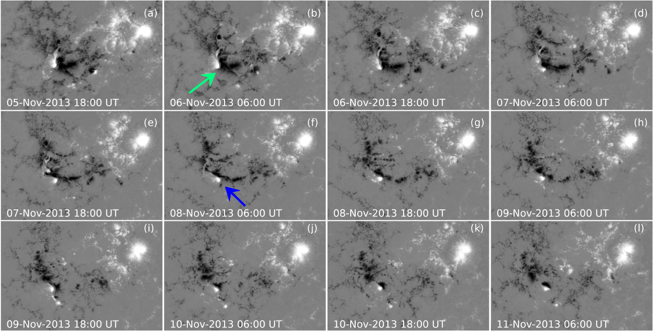
Figure 1: Selected images of the normal component of the photospheric magnetic field of AR11890 taken by the HMI during the interval studied in this paper. The green arrow marks the area where intense magnetic flux decay occurred while the blue arrow shows the location of the parasitic positive polarity at a later stage during the flux decay episode. The field of view of each panel is $571\arcsec\times 387\arcsec$.

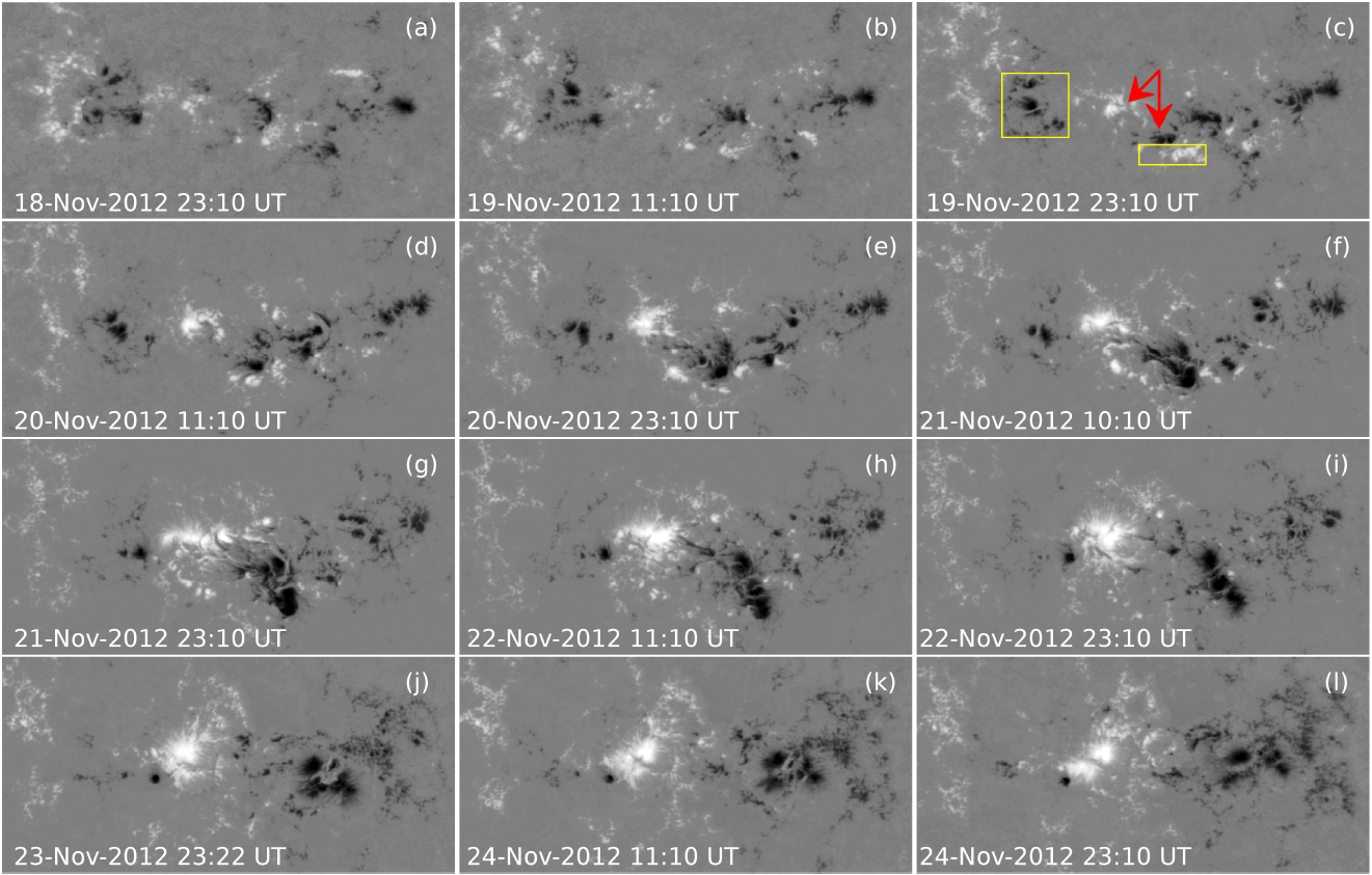
Figure 2: Same as Fig. 1 but for AR11618. The red arrows indicate sites of major flux emergence while the yellow boxes enclose areas whose magnetic flux was affected by cancellation. The field of view of each panel is $611\arcsec\times 291\arcsec$.

The uncertainties of the CB-method results have been discussed by Georgoulis et al. (2012b). They are usually rather small and for this reason we did not use them; instead, we use the standard deviations of the moving five-point (48-minute) averages of the $H$ and $E_{f}$ curves, that tend to represent more sizable uncertainties (see also Moraitis et al., 2021). The uncertainties of all quantities that are produced from either $H$ or $E_{f}$ (see Sect. 4.3, 4.4 and 5) were also calculated by evaluating the standard deviations of their moving five-point averages.

3.2 Helicity and energy flux integration method

The formulas for the magnetic helicity and magnetic energy fluxes across the photospheric surface, $S$ are

$$\dfrac{dH}{dt}\Bigg{|}_{S}=2\int_{S}(\mathbf{A}_{P}\cdot\mathbf{B}_{t})V_{\perp n}dS-2\int_{S}(\mathbf{A}_{P}\cdot\mathbf{V}_{\perp t})B_{n}dS$$ (3)

$$\frac{dE}{dt}\Bigg{|}_{S}=\frac{1}{4\pi}\int_{S}B^{2}_{t}V_{\perp n}dS-\frac{1}{4\pi}\int_{S}(\mathbf{B}_{t}\cdot\mathbf{V}_{\perp t})B_{n}dS$$ (4)

(Berger, 1984, 1999; Kusano et al., 2002) where $\mathbf{A}_{P}$ is the vector potential of the potential magnetic field $\mathbf{B}_{P}$, $\mathbf{B}_{n}$ and $\mathbf{B}_{t}$ are the normal and tangential components of the photospheric magnetic field, and $V_{\perp n}$ and $\mathbf{V}_{\perp t}$ are the normal and tangential components of the velocity $V_{\perp}$ which is perpendicular to the magnetic field lines (cross-field velocity). The first terms of Eqs. (3) and (4) correspond to the contribution from magnetic flux emergence while the second terms correspond to the contribution from photospheric shuffling.

The velocity field involved in Eqs. (3) and (4) was computed with the Differential Affine Velocity Estimator for Vector Magnetograms (DAVE4VM; Schuck, 2008) algorithm, applied to sequential pairs of the $B_{x}$, $B_{y}$, and $B_{z}$ datacubes (see Liu & Schuck, 2012; Liu et al., 2014, for details). The velocities were further corrected by removing their components which are parallel to the magnetic field (see Liu & Schuck, 2012; Liu et al., 2014). The helicity flux was computed by integrating the so-called $G_{\theta}$ helicity flux density proxy (see Pariat et al., 2005, 2006) over the area covered by the magnetograms. $G_{\theta}$ is given by

$$G_{\theta}({\bf x})=-\dfrac{B_{n}}{2\pi}\int_{S^{\prime}}\frac{d\theta({\bf r})}{dt}B^{\prime}_{n}dS^{\prime}$$ (5)

where $d\theta/dt$ is the relative rotation rate of two elementary magnetic fluxes located at $\bf{x}$ and $\bf{x\arcmin}$ and $\bf{r}=\bf{x}-\bf{x\arcmin}$. This rate does not depend on the choice of the direction that is used for the definition of $\theta$. The $G_{\theta}$ maps were derived by applying the fast Fourier Transform method of Liu & Schuck (2013).

The accumulated changes in magnetic energy, $\Delta E$, and helicity, $\Delta H$, were calculated by integrating the magnetic energy and helicity fluxes over time. Following Thalmann et al. (2021) the $\Delta E$ and $\Delta H$ time profiles have been constructed by using reference magnetic energies and helicities that are equal to the corresponding average values of these quantities deduced from the CB method over the first two hours of observations.

All magnetogram pixels were used for the calculation of the magnetic helicity and energy fluxes. For test purposes, in a few representative cases we took into account only those pixels that were used for the CB-method calculations (see Sect. 3.1), and found magnetic helicity and energy fluxes which were very close (differences of less than 1%) to the ones obtained by the entire magnetograms’ field of view.

4 Long-term evolution of the magnetic helicity and energy of the ARs

4.1 Photospheric magnetic morphology

Let us first discuss the evolution of the photospheric configurations of the two ARs (see Figs. 1 and 2, and also the associated movies).

AR11890 was classified as a $\beta\gamma\delta$ active region and produced several major flares and CMEs in early November 2103. One of its eruptive events has been presented by Xu et al. (2016) and Gupta et al. (2021) while selected properties of the magnetic helicity injection rate in AR11890 have been discussed by Korsós et al. (2020).

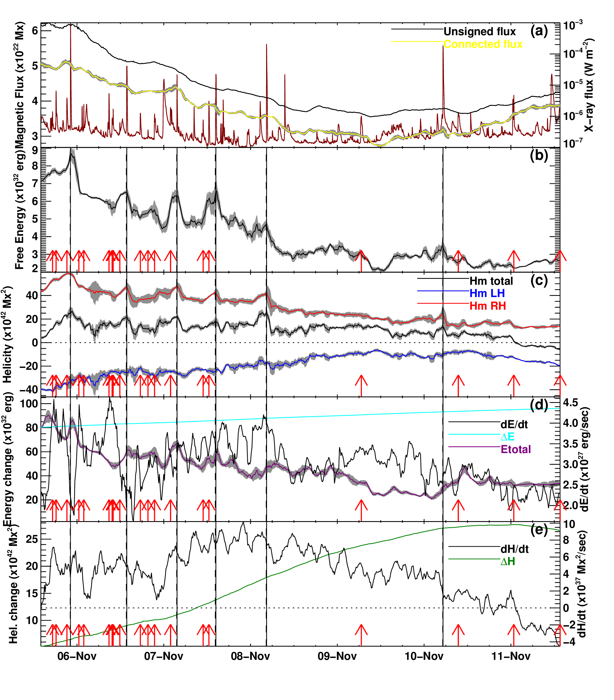
Figure 3: Time profiles of magnetic properties of AR11890. (a) Total unsigned magnetic flux, unsigned connected magnetic flux used in the CB-based method, and X-ray flux from the GOES 1-8 Å channel (black, yellow, and maroon curves, respectively). (b) Free magnetic energy. (c) Right-handed, left-handed, and net helicity (red, blue, and black curves, respectively). (d) Magnetic energy injection rate, the corresponding accumulated energy, $\Delta E$, and the total energy from the CB method (black, cyan, and purple curves, respectively). (e) Helicity injection rate and the corresponding accumulated helicity, $\Delta H$, (black and green curves, respectively). In this and subsequent figures, vertical straight lines indicate the start and peak times of M- and X-class flares (all of them being eruptive) while arrows indicate the peak time of C-class flares (all of them being confined). The gray bands show the error bars.

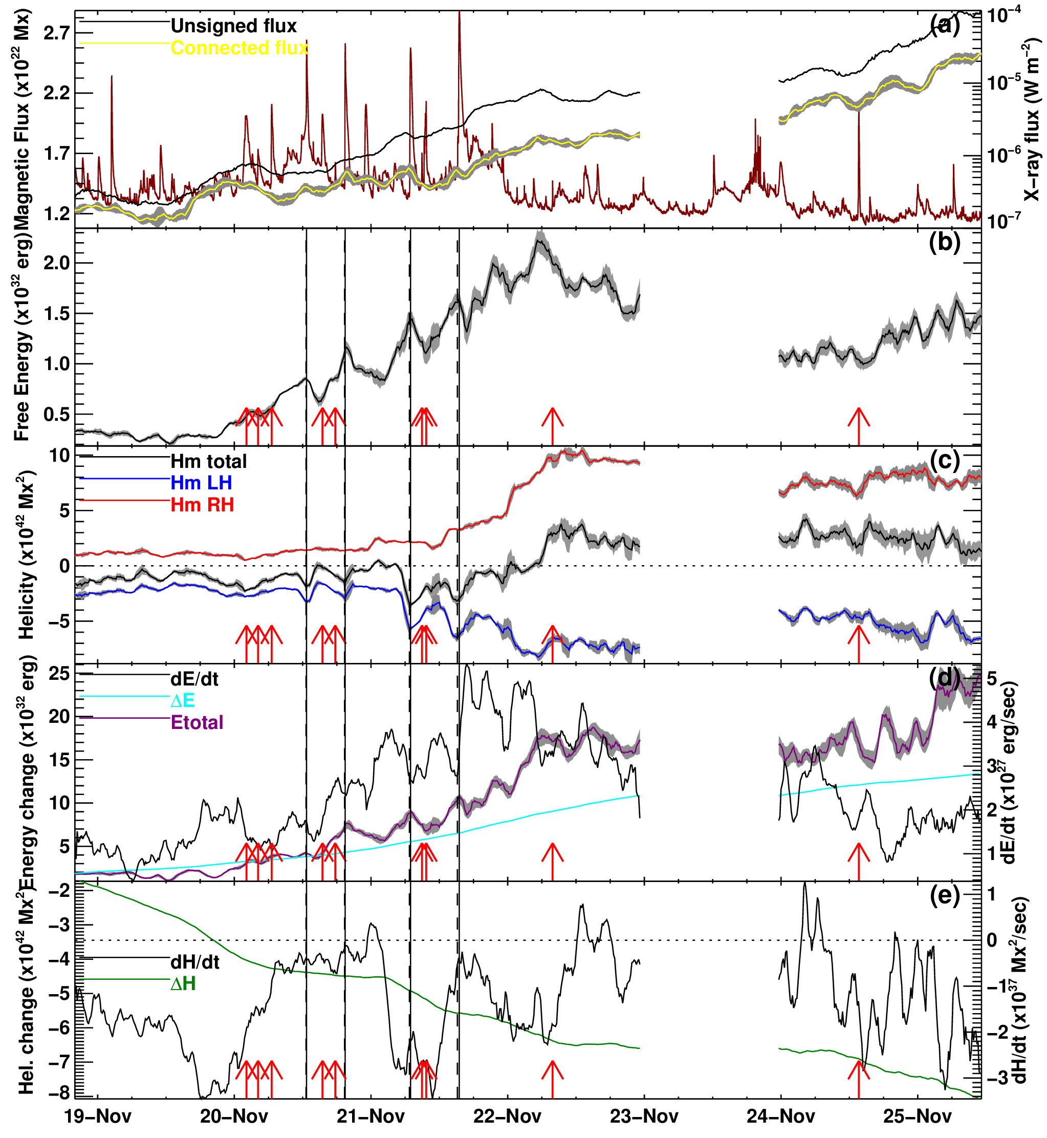
Figure 4: Same as Fig. 3 but for AR11618.

The evolution of the photospheric magnetic configuration of the AR is presented in Fig. 1, and in the associated movie. At the beginning of observations (panel a) its major components are a large fairly unperturbed preceding sunspot with positive polarity in the north-west part of the AR and a large bipolar following sunspot complex consisting of a massive negative polarity and a smaller elongated positive polarity patch (see the green arrow in panel b). Smaller patches of positive and negative polarity, associated with smaller sunspots and pores, are also located between these two large sunspots.

At the first stages of the observations (panels a-h) the preceding positive sunspot does not change much. However, magnetic flux decay is observed in the eastern part of the AR between the elongated positive-polarity patch and the more massive negative polarity. As a result the massive eastern negative polarity gradually weakens (panels a-h) and attains an elongated shape. At the same time due to shearing motions the eastern patch of positive polarity gradually moves southwest of its initial location (compare the positions of the arrows in panels b and f). From about November 9 09:30 UT onward, new positive magnetic flux emerges in the central part of the AR (see panels i-l) while flux decay, albeit at a slower rate than before, continues to takes place in the eastern part of the AR. Furthermore, the large positive preceding sunspot appears to gradually develop a double umbra configuration (panels h-l).

The above trends are also illustrated in Fig. 3(a) where we show the evolution of the total unsigned magnetic flux (that is, the algebraic sum of the positive magnetic flux and the absolute value of the negative magnetic flux) of AR11890. The average flux decay rate in the interval defined from the start of observations and the time when the flux attains its minimum value (November 9 09:36 UT) is $7.9\times 10^{16}$ Mx s^-1. This value is almost an order of magnitude larger than the largest cancellation rates measured by Yardley et al. (2018) in 20 small bipolar ARs. The corresponding decrease in magnetic flux is $2.6\times 10^{22}$ Mx (in Fig. 3(a) compare the initial value of the unsigned flux with its minimum value) which amounts to about 40% of the AR’s initial unsigned flux. This percentage lies on the high end of flux cancellation percentages calculated by Green et al. (2011), Baker et al. (2012) and Yardley et al. (2016, 2018). The subsequent flux emergence phase is accompanied by cancellation and therefore the calculation of the average flux emergence rate from the time profile of the unsigned flux is not reliable.

Figure 2 and the associated movie show the evolution of the normal component of the photospheric magnetic field of AR 11618. It was an eruptive AR which exhibited multipolar photospheric magnetic configuration throughout the interval we studied.

From about November 19 11:10 UT until the data gap (panels b-i) significant emergence of both positive and negative polarity flux takes place primarily at the central part of the AR. In panel (c) the major locations of flux emergence are marked with the red arrows; the left arrow shows the site of positive flux emergence while the right one shows the site of negative flux emergence. As usually happens in the emergence phase (e.g. see van Driel-Gesztelyi & Green, 2015) the magnetic polarities separate over time. Their separation brought them close to opposite polarity pre-existing fluxes. In both cases the proximity of opposite polarity fluxes gave rise to cancellation which resulted in the gradual weakening of the fluxes that are enclosed in the yellow boxes of panel (c). The combination of the above evolutionary trends resulted in the gradual formation (see panels c-i) of two major sunspot groups. The first was located in the south-central part of the AR and consisted of three negative polarity sunspots with a common penumbra. The second was located in the central-eastern part of the AR and contained positive polarity sunspots with the exception of its small easternmost member which featured negative polarity. A new episode of flux emergence was captured after the data gap (panels i-l) which is resulted in the enhancement of the magnetic flux at the central-eastern part of the AR.

The time profile of the unsigned magnetic flux in AR11618 appears in Fig. 4(a), and reflects the major evolutionary trends discussed above. However, the fact that before the data gap flux emergence is accompanied by cancellation (although not as strong as flux emergence) makes the calculation of the corresponding average emergence rate from the time profile of the unsigned flux not reliable. After the data gap, cancellation has been largely suppressed and the corresponding flux emergence rate is $4.5\times 10^{16}$ Mx s^-1. This value is consistent with previous statistical studies (e.g. Otsuji et al., 2011; Kutsenko et al., 2019; Liokati et al., 2022).

4.2 Diagnostics of evolution from magnetic helicity and energy

In Fig. 3 and 4 we present the evolution of the free magnetic energy (panels b) and helicity (panels c) of ARs 11890 and 11618, respectively. In all free energy and helicity curves we show the 48-min averages of the actual curves in order to clearly assess the long-term evolution of both quantities. This can be described as the superposition of slowly varying backgrounds featuring characteristic time scales of more than one day with shorter localized peaks which, in several cases, are associated with eruption-related changes.

In more detail, the first phase of the evolution of $E_{f}$’s slowly varying component in AR11890 involves its decrease from the start of the observations until about 09 November 2013 09:36 UT where it gets its minimum value. The average rate of change referring to this period is $-1.4\times 10^{27}$ erg s^-1. Then it starts rising for about four hours and attains an extended plateau with an overall weak decreasing trend; this second phase lasts for about 25 hours. Subsequently a slow rise follows (rate of change of $3.2\times 10^{26}$ erg s^-1) until the end of the observations. A comparison of the $E_{f}$ curve with the black and yellow curves of Fig. 3(a) shows that these trends largely follow the large-scale temporal trends of both the total unsigned magnetic flux, $\Phi$, and the total magnetic flux that participates in the CB-method’s connectivity matrix, $\Phi_{conn}$ (hereafter referred to as connected flux; see Georgoulis et al., 2012b). During the flux decay phase the unsigned magnetic flux decreases and so does the connected flux which results to the decrease of free energy while the opposite happens during the later flux emergence phase. The good correlation of the $E_{f}$ with $\Phi$ and $\Phi_{conn}$ is quantified by their linear (Pearson) and rank-order (Spearman) correlation coefficients which are 0.92-0.88 and 0.80-0.74 for the $\Phi-E_{f}$ and $\Phi_{conn}-E_{f}$ pairs, respectively. Even higher ($\gtrsim 0.90$) correlation coefficients are achieved if we consider the flux decay phase and the flux emergence phase separately. Furthermore, very similar correlation coefficients are derived if the $E_{f}$ timeseries is replaced by the total magnetic energy timeseries (see Fig. 3d).

The time profiles of AR11890’s helicity (total, right-handed, and left-handed) are presented in Fig. 3(c). Substantial values of both right-handed and left-handed helicity are present throughout the observations. The AR’s net helicity is right-handed (i.e. it has positive sign) from the start of the observations until about 11 November 2013 01:34 UT. Then it changes sign and becomes left-handed (i.e. with a negative sign) until the end of the observations. This happens due to a combination of two reasons. (1) During the flux decay both the right-handed and left-handed helicity decrease (in absolute values) because of the decrease of the unsigned and connected flux. However, the right-handed helicity decreases at a rate ($-6.3\times 10^{37}$ Mx² s^-1) which is higher than the rate at which the left-handed helicity decreases ($5.5\times 10^{37}$ Mx s^-1). (2) After $\Phi_{conn}$’s minimum and until the end of the observations, the slowly-varying component of the right-handed helicity does not show appreciable changes with time whereas the absolute value of the left-handed helicity increases at a rate of $3.7\times 10^{38}$ Mx² s^-1. The net helicity change of sign explains its poor correlation with both the unsigned and connected fluxes (0.38 and 0.29 for the linear correlation coefficient and 0.37 and 0.33 for the rank-order correlation coefficient). On the other hand, the right-handed and even more so the left-handed helicities show much better correlation with the unsigned and connected flux (linear and rank-order correlation coefficients in the range 0.68 to 0.93). Another simple explanation could be that the flux emerged from around midday on November 10 could be oppositely helical. This is also corroborated by Fig. 3(e).

The free energy and helicity evolution in AR11618 appear in Fig. 4(b) and (c), respectively and can be described as follows. The free energy from the start of the observations until about 19 November 2012 21:00 UT does not change appreciably. Then it increases until about 22 November 05:22 at a rate of $8.5\times 10^{26}$ erg s^-1. This phase coincides with much of the flux emergence episode before the data gap which led to the increase of both the unsigned and connected flux (see panel a). Subsequently, $E_{f}$ decreases from about noon UT on November 22 until the data gap. This decrease does not match the corresponding evolution of the connected flux which shows a plateau. This behavior of $\Phi_{conn}$ is closer to the corresponding behavior of the total energy, $E_{tot}$ (see Fig. 4(d)). After the data gap both $E_{f}$ and $E_{tot}$ fluctuate for about 15.5 hours around values of 1.1 and $15.5\times 10^{32}$ erg, respectively, and then increase until the end of the observations. This behavior is broadly consistent with that of $\Phi_{conn}$ although the $E_{f}$ increase is milder. Overall, the values of the linear and rank-order correlation coefficients are in the range 0.6-0.7 for the entire evolution of the $\Phi_{conn}-E_{f}$ pair. This correlation is lower than the one in AR11890 and results from the decrease of the contribution of the free energy to the total magnetic energy budget after the fourth major flare (this will become evident in the discussion of the $E_{f}/E_{tot}$ time profile in Sect. 4.4). On the other hand, the correlation coefficients of the $\Phi_{conn}-E_{tot}$ pair are higher than 0.9. This suggests that in AR11618 the connected flux correlates better with the global magnetic field evolution (see also Tziotziou et al., 2013).

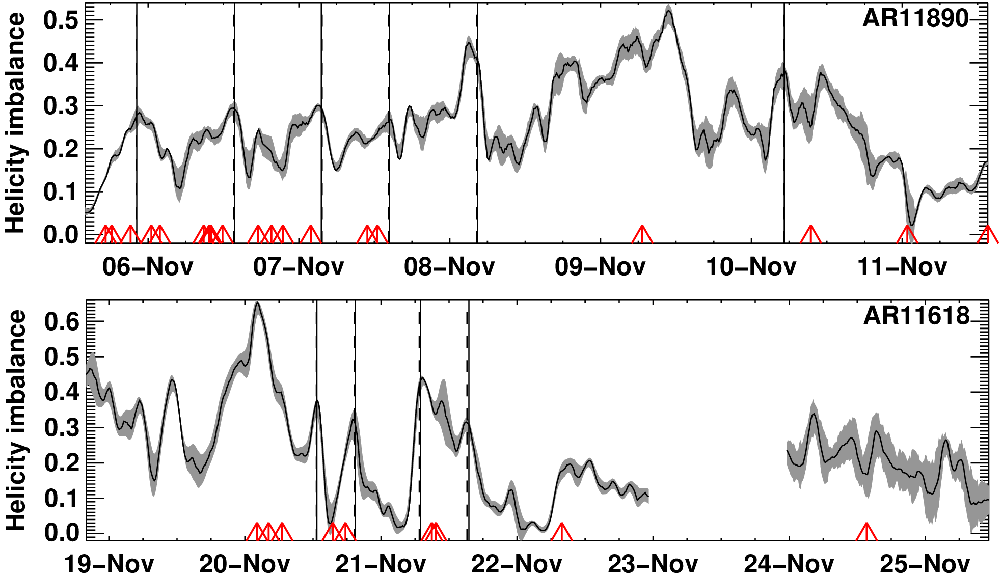
Figure 5: Evolution of the helicity imbalance parameter, $h_{imb}$ (see text for details) for AR11890 (top panel) and AR11618 (bottom panel).

AR11618 shows predominantly (but weakly) left-handed net helicity from the start of the observations until about the time when the free energy gets its maximum value (compare panels (b) and (c) of Fig. 4). Then the net helicity changes sign and becomes right-handed until the end of the observations. The time interval of left-handed net helicity prior to the data gap is interrupted by three short excursions (centered at 20 November 14:46, 21 November 01:58, and 22 November 00:46) where the net helicity becomes right-handed. Both the left-handed and right-handed helicity do not show appreciable long-term variability from the start of the observations until about the end of November 20 although shorter-term changes associated with two of the four M-class flares are registered in this interval (see Sect. 5). Then both signed components of helicity increase by absolute value; the left-handed helicity increases faster than the right-handed helicity in the interval until 21 November 23:22 (increase rates of 4.3 and $3.7\times 10^{37}$ Mx² s^-1, respectively) and this combined with the initial predominance of the left sense results in the left-handed sign of the net helicity. Subsequently, the situation is reversed in the interval until 22 November 13:22 (the corresponding rates of change are $2.3\times 10^{37}$ and $1.1\times 10^{38}$ Mx² s^-1) resulting in the sign change of the net helicity at 22 November 04:22. Then both signed components of helicity do not show appreciable long-term changes until the data gap.

After the data gap, the right-handed helicity fluctuates around a value which is smaller than its value before the data gap ($\sim$8.0 versus $\sim$$9.4\times 10^{42}$ Mx²). The left-handed helicity emerges from the data gap with a smaller absolute value than before (-4.2 versus $-7.5\times 10^{42}$ Mx²) which is also smaller in amplitude than the corresponding value of the right-handed helicity. The long-term amplitude increase of the left-handed helicity until the end of the observations (at a rate of $\sim$$-1.9\times 10^{37}$ Mx² s^-1) is not adequate to balance the increase of the right-handed helicity and hence the net helicity keeps its positive sign. As in AR11890, the correlation between the net helicity and the connected flux is poorer (linear and rank-order correlation coefficients of 0.60 and 0.65) than the resulting correlation of the left- or right-handed helicity with the connected flux (coefficients in the range 0.70-0.88).

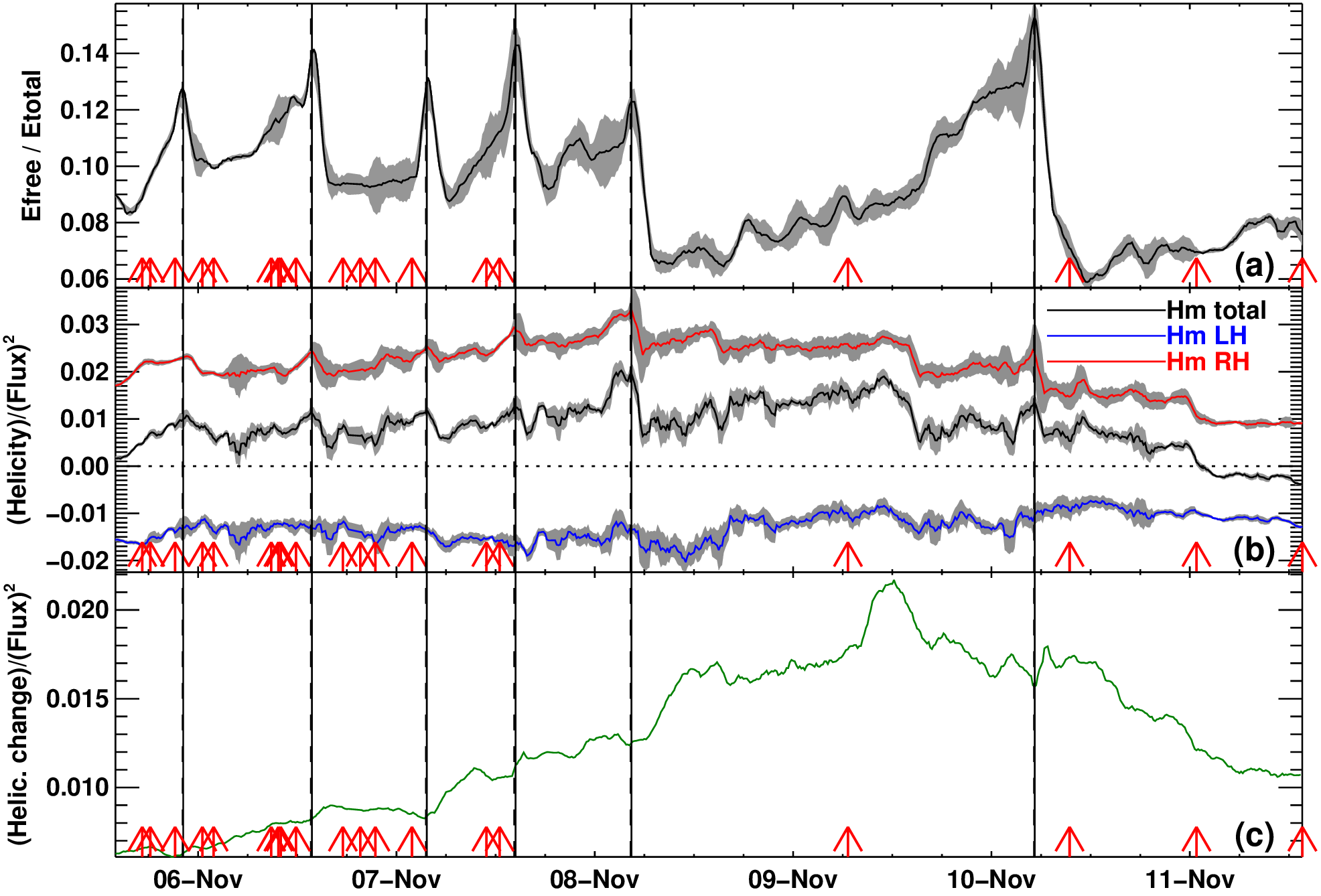
Figure 6: Time profiles of normalized magnetic quantities for AR11890. (a) Ratio of the free magnetic energy to the total magnetic energy. (b) Ratios of the right-handed, left-handed, and net helicity to the connected magnetic flux squared (red, blue, and black curves, respectively). (c) Ratio of the accumulated helicity (resulting from the helicity injection rate of the flux-integration method) to the connected magnetic flux squared.

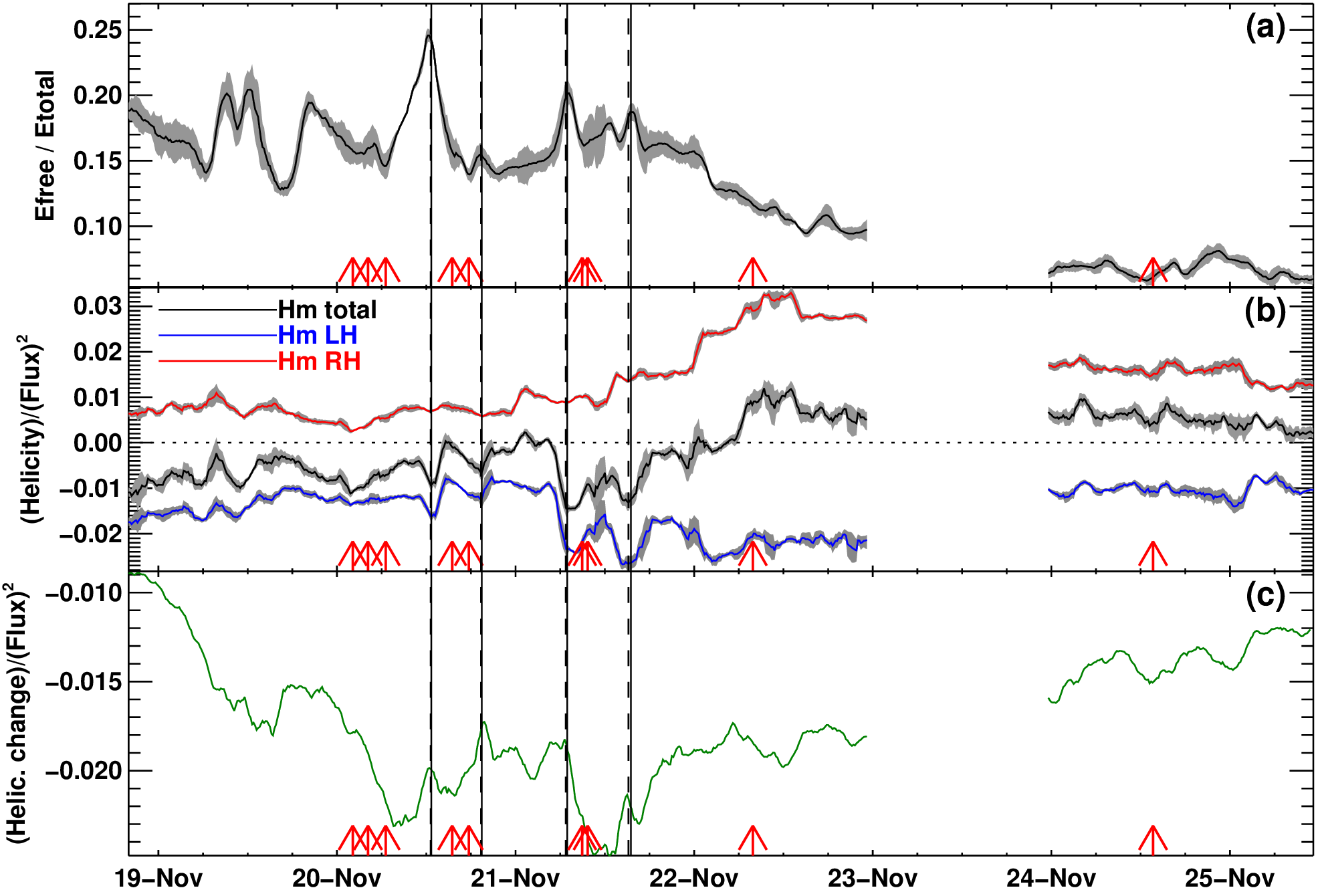
Figure 7: Same as Fig. 6 but for AR11618.

A worth mentioning property of the calculations presented in Figs. 3 and 4 is that both ARs contain substantial budgets of free magnetic energy during much of the observations. In AR11890 the free energy is amply above the threshold of $4\times 10^{31}$ erg for the occurence of major flares (see Tziotziou et al., 2012) throughout the observations and reaches a maximum value of $8.7\times 10^{32}$ erg. The same is true for AR11618 after 19 November 2012 23:22; here the free energy reaches maximum value of $2.2\times 10^{32}$ erg. The signed terms of the net helicity also exhibit adequate budgets (that is, above the threshold of $2\times 10^{42}$ Mx² for the occurrence of major flares; Tziotziou et al., 2012) throughout the observations. In AR11890 the positive and negative components of the helicity reach maximum values of $5.8\times 10^{43}$ Mx² and $-4.1\times 10^{43}$ Mx², respectively. The corresponding maximum values for AR11618 are $1.0\times 10^{43}$ Mx² and $-8.2\times 10^{42}$ Mx².

4.3 Imbalance in the signed components of the helicity budgets

A common feature of the helicity budgets of both ARs is that throughout their evolution they contain comparable amounts of both right-handed and left-handed helicity. This can be quantified by introducing a helicity imbalance parameter, $h_{imb}$, (see also Georgoulis et al., 2009) as

$$h_{imb}=\frac{|H|}{H_{+}+|H_{-}|}$$ (6)

where $H$, $H_{+}$, and $H_{-}$ denote the net, right-handed, and left-handed helicity, respectively. $h_{imb}$ can range from 0 (indicating perfect balance between the positive and negative helicity) to 1 (indicating perfect dominance of a particular sense of helicity). The evolution of $h_{imb}$ for both ARs is presented in Fig. 5. The plots indicate that during much of the observations the value of $h_{imb}$ was below 0.5. The ARs acquire the minimum value of $h_{imb}$, which is zero, at the times when the net helicity changes sign (see the discussion in Sect. 4.2). The temporal average of $h_{imb}$ was $0.25\pm 0.09$ for AR11890 and $0.23\pm 0.14$ for AR11618.

Case studies (e.g. Pariat et al., 2006; Georgoulis et al., 2012b; Tziotziou et al., 2013; Vemareddy, 2017, 2019; Thalmann et al., 2019; Dhakal et al., 2020) indicate that most eruptive ARs feature a clear prevelance of one signed helicity component over the other that does not change in the course of observations. However, there are observations of ARs whose helicity sign changes during observations, but almost always these are non-eruptive ARs (e.g. Vemareddy & Démoulin, 2017; Vemareddy, 2021, 2022), although reports about one eruptive AR also exist (see Georgoulis et al., 2012b; Thalmann et al., 2021). The existence of a dominant sense of helicity in most eruptive ARs throughout their observations is also supported either directly (e.g. LaBonte et al., 2007; Georgoulis et al., 2009; Liokati et al., 2022) or indirectly (e.g. Tziotziou et al., 2012) by statistical studies. On the other hand, explicit reports about the relative contribution of the positive and negative helicity to the net helicity budget of ARs are rather scarce. Tziotziou et al. (2014) found that the ratio between the $H_{+}$ and the $H_{-}$ terms of the net helicity in the quiet Sun ranges from 0.32 to 2.31 with an average of 1.06. The temporal averages of $h_{imb}$ that we found for our two ARs correspond to ratios of $H_{+}/H_{-}$ of $1.68\pm 0.46$ and $0.94\pm 0.45$ for ARs 11890 and 11618, respectively. Therefore, the helicity imbalance of our ARs is similar to that of the quiet Sun, which is more exceptional, rather than nominal, for active regions.

4.4 Diagnostics of evolution from magnetic helicity and energy normalized parameters

In order to put the free magnetic energy and helicity computations in the two active regions on the same footing, we calculated the following normalized parameters: the ratio of the free magnetic energy to the total magnetic energy, $E_{f}/E_{tot}$, as well as the magnetic-flux normalized net, right-handed, and left-handed helicity ($H/\Phi_{conn}^{2}$, $H_{+}/\Phi_{conn}^{2}$, and $H_{-}/\Phi_{conn}^{2}$, respectively). These quantities have often been used as proxies to quantify the nonpotentiality of the magnetic field of ARs as well as their eruptive potential (e.g. Pariat et al., 2017; Thalmann et al., 2019, 2021; Gupta et al., 2021). $E_{f}/E_{tot}$ quantifies the percentage of total magnetic energy that can be converted to other forms in flares and CMEs. As a first approximation, the $H/\Phi_{conn}^{2}$ parameter reflects the complexity of the magnetic field structure while $H$ reflects both the structure and the flux budget; this is because the helicity of an isolated flux tube with magnetic flux $\Phi$ which is uniformly twisted with $N$ turns is simply $N\Phi^{2}$.

The above normalized parameters for ARs 11890 and 11618 appear in Figs. 6 and 7, respectively. We note that $E_{f}/E_{tot}$ acquires values in the range 0.06-0.25 which are consistent with previous results (e.g. see Metcalf et al., 1995; Guo et al., 2008; Thalmann et al., 2008; Malanushenko et al., 2014; Aschwanden et al., 2014; Gupta et al., 2021). In both ARs the long-term evolution of the $E_{f}/E_{tot}$ curves is different from those of the $E_{f}$ curves. These different trends can be understood in terms of the varying contribution of the free energy to the budget of the total magnetic energy of the active regions. In AR11890 there is no conspicuous decrease of $E_{f}/E_{tot}$ during much of the flux decay phase while in AR11618 there is no conspicuous increase of $E_{f}/E_{tot}$ during the flux emergence phase before the data gap. In AR11890 this happens because of the milder temporal decrease of $E_{tot}$ than $E_{f}$ (compare panels (b) and (d) of Fig. 3) while in AR11618 the reason is the milder temporal increase of $E_{tot}$ than $E_{f}$ (compare panels (b) and (d) of Fig. 4). Furthermore, in AR11890 $E_{f}/E_{tot}$ gradually increases in the interval starting after its downward jump that occurred after the fifth major flare and ending at the time of the sixth flare. Then it exhibits a sharp decrease for about 7.5 hours before resuming to show a mild increase until the end of the observations. In AR11618 $E_{f}/E_{tot}$ starts decreasing after the fourth major flare and until the end of the observations.

Going to the magnetic-flux normalized helicities (panels b of Figs. 6 and 7) we note that in both ARs $H_{\pm}/\Phi_{conn}^{2}$ possess absolute values in the range 0.003-0.032 which are consistent with results presented in previous publications (e.g. Thalmann et al., 2019, 2021; Gupta et al., 2021; Liokati et al., 2022). In AR11890 there is a gradual increase of the $H_{+}/\Phi_{conn}^{2}$ curve from the start of the observations until the fifth major flare which is followed by a gradual decrease until the end of the observations. On the other hand the $H_{-}/\Phi_{conn}^{2}$ curve is flatter than the $H_{-}$ curve (compare panel b of Fig. 6 with panel c of Fig. 3). These trends may reflect the gradual build-up of right-handed twist in the AR from the start of the observations until the fifth major flare; after that time it decreases with a rate which is faster than the decrease of the left-handed twist (Sect. 4.2) resulting in the eventual sign change of the magnetic-flux normalized net helicity. In AR11618 the magnetic-flux normalized helicities show trends which are similar to those of their parent parameters (compare panel c of Fig. 4 with panel b of Fig. 7).

In agreement with the discussion in Sect. 4.2, in both ARs all major flares (which are all eruptive; see Sect. 2) are associated with well-defined peaks of the helicity and free energy normalized parameters (see Figs. 6 and 7). We will return to this significant finding in Sect. 5.

Several authors (e.g. Berger, 2003; Moraitis et al., 2014; Pariat et al., 2017; Linan et al., 2018, 2020) have decomposed the total helicity into a current-carrying component and a volume-threading component (that is, the component of helicity related to the field threading the boundary of the volume where the helicity calculation is performed). However, the CB method cannot provide such decomposition and therefore we cannot test the popular parameter (see Sect. 1 for references) defined by the ratio of current-carrying helicity to the total helicity.

4.5 Comparison of results from the connectivity-based and flux-integration methods

Prior to a detailed discussion, the following notes are in order for the results from the flux-integration method. First, a direct comparison of the time profiles of the quantities provided by the two methods is not straightforward because the flux-integration method yields the accumulated magnetic energy, $\Delta E$, and helicity, $\Delta H$, over certain times, while the CB method yields their instantaneous budgets, including changes thereof. In essence, the CB method provides pseudo-timeseries (that is, timeseries in which each point is independent of the one before or the one after) contrary to the flux integration method. Second, the flux-integration method, in contrast to the CB method, provides the total magnetic energy without separating into free and potential components (e.g. Liu et al., 2014). Third, although all helicity flux density proxies eventually should yield the same net helicity flux, its distribution between its signed components may vary according to the flux density proxy that was used (Pariat et al., 2005, 2006; Dalmasse et al., 2014). These authors, as well as Dalmasse et al. (2018), have pointed out that the $G_{\theta}$ proxy may yield fake helicity flux density polarities. This is why studies, with this one among them, present only net rates or integrated helicities from the flux-integration method. Fourth, the uncertainties of the magnetic energy injection rate, $dE/dt$, and the helicity injection rate, $dH/dt$, were calculated for selected representative values of these quantities (that is, at a nonuniform sampling) by using the Monte Carlo experiment approach as in Liokati et al. (2022) (see also Liu & Schuck, 2012; Liu et al., 2014). They never exceeded 20%. Furthermore, the corresponding uncertainties in the accumulated quantities, $\Delta E$ or $\Delta H$, were about two orders of magnitude smaller than the pertinent accumulated quantity. In the pertinent curves of Figs 3(d-e), 4(d-e), 6(c), and 7(c) we do not mark the uncertainties of the flux integration results because of their small values and nonuniform sampling.

The time profiles of the magnetic energy and helicity injection rates from the flux-integration method as well as the corresponding accumulated quanties are presented in panels (d) and (e), respectively, of Figs 3 (for AR11890) and 4 (for AR11618). In panels (c) of Figs. 6 and 7 we also show the magnetic-flux normalized profiles of the accumulated $\Delta H$ from the flux-integration method in ARs 11890 and 11618, respectively.

In both ARs, both $dE/dt$ and $dH/dt$ exhibit significant short-term fluctuations lasting up to 10 hours which are superposed on their longer-term evolution. Most of these fluctuations do not seem directly relevant to any of the major flares of the ARs. Therefore, in most cases, our results are not necessarily consistent with previous reports of occasional good correlation between helicity injection and soft X-ray activity (e.g. Maeshiro et al., 2005). However, we note that Korsós et al. (2020) have advocated for periodicities of 8 and 28 hours prior to three X-class flares of AR11890.

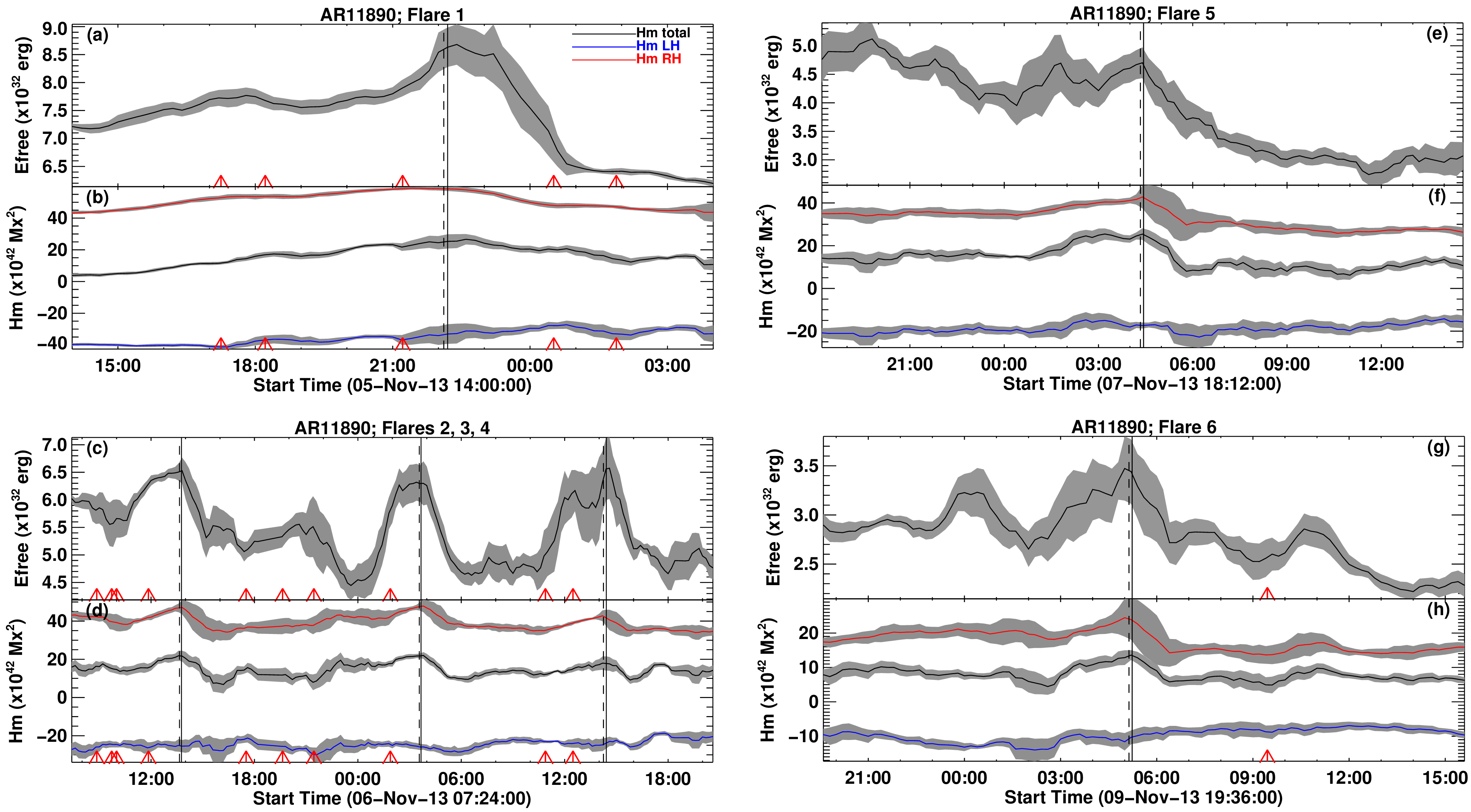
Figure 8: Stack of plots showing the evolution of free magnetic energy (top plot) and of the net, right- and left-handed helicity budgets (bottom plot) for each of the six major eruptive flares in AR11890 a few hours before and after the events. The first (X3.3) flare is shown in plots (a, b), flares 2, 3 and 4 (M3.8, M2.3 and M2.4, respectively) are shown in plots (c, d), the fifth flare (X1.1) is shown in plots (e, f), while the sixth flare (X1.1) is shown in plots (g, h).

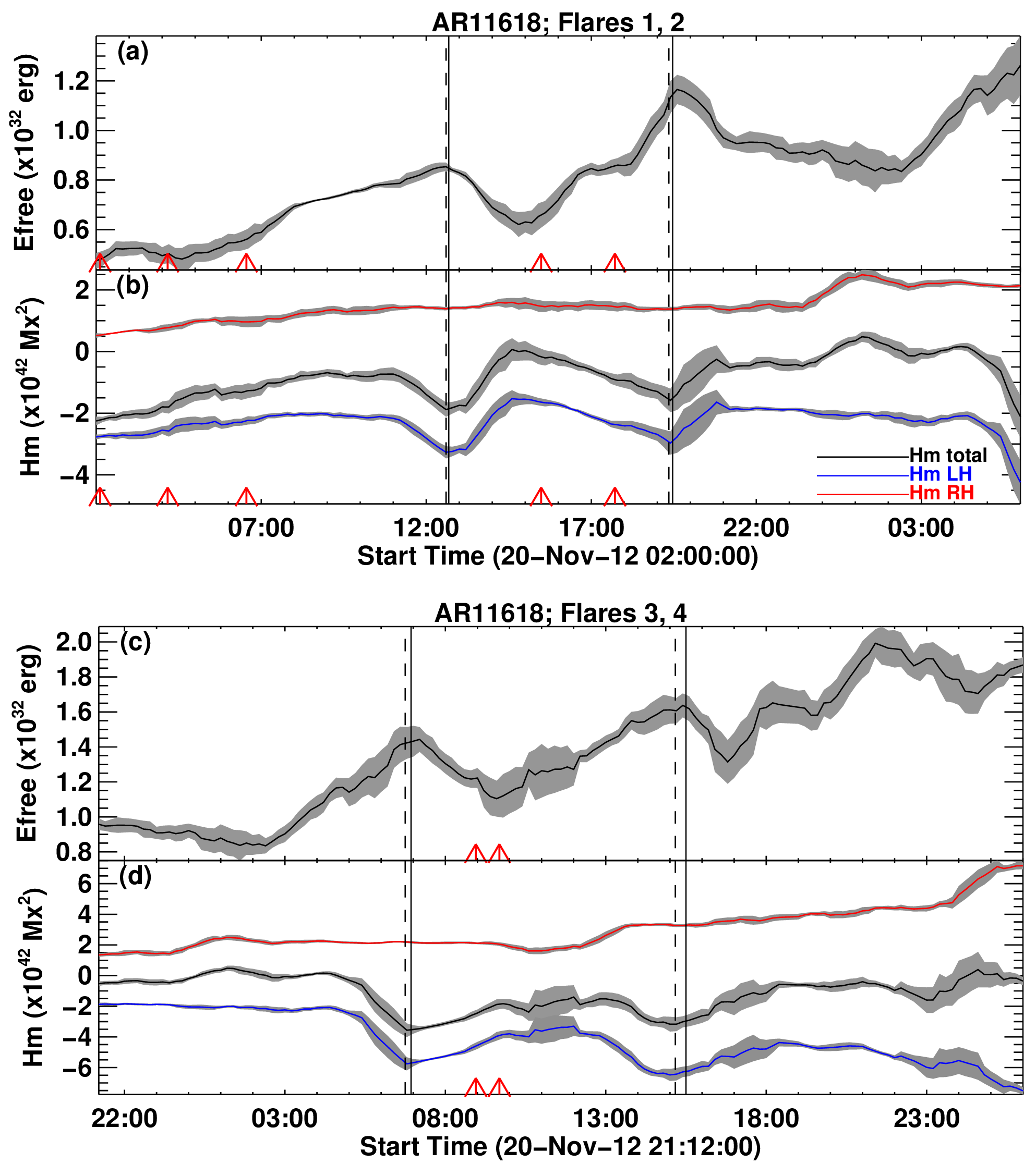
Figure 9: Stack of plots showing the evolution of free magnetic energy (top plot) and of the net, right- and left-handed helicity budgets (bottom plot) for each of the four major eruptive flares in AR11618 a few hours before and after the events. The first and second flares (M1.7 and M1.6, respectively) are shown in plots (a, b) while the last two flares (M1.4 and M3.5, respectively) are shown in plots (c, d).

In AR11890, and in agreement with the CB-method results, $dH/dt$ is positive for much of the observations. It changes sign for the first time some 10 hours prior to the sign reversal of the instantaneous helicity. This 10-hour interval is characterized by very small $dH/dt$ values and multiple changes of its sign. Subsequently, the $dH/dt$ sign stays negative until the end of the period we studied, in agreement with both the sign and the overall weak decreasing trend of the instantaneous helicity (compare panels (c) and (e) of Fig. 3). Contrary to the $E_{tot}$ time profile from the CB method, the $\Delta E$ curve steadily increases with time because it is constructed by the accumulation of positive values (see Fig. 3(d)). The $\Delta H$ curve shows a similar behavior until around the time of the sign reversal of the helicity. Then it shows a plateau and subsequently declines until the end of the observations because negative values start accumulating into the helicity budget. However, these negative budgets are not sufficient to change its positive sign. At the end of the observations $\Delta H$ has acquired a value of $2.6\times 10^{43}$ Mx² which is a factor of 1.8 higher than the corresponding instantaneous budget of $H_{+}$.

The $\Delta H/\Phi_{conn}^{2}$ curve of Fig. 6(c) exhibits richer structure than the $\Delta H$ curve of Fig. 3(e) which reflects the competition between the increasing $\Delta H$ evolution and the more complicated evolution of the $\Phi_{conn}$ time series We also note that the $H_{+}/\Phi_{conn}^{2}$ and $\Delta H/\Phi_{conn}^{2}$ values at the end of the observations are similar (differences of 17%).

In AR11618 $dE/dt$ increases at least until about the fourth major flare (see Fig. 4(d)). The evolution of the corresponding accumulated energy, $\Delta E$ is qualitatively similar to that of the instantaneous total magnetic energy, $E_{tot}$, from the CB method. This could not happen if $E_{tot}$ were decreasing with time (see the relevant discussion about AR11890). At the end of the observations, $E_{tot}$ has acquired a value of $2.4\times 10^{33}$ erg while $\Delta E$ a value of $1.3\times 10^{33}$ erg.

The situation is more complicated regarding the comparison of the helicities from the two methods in AR11618. $dH/dt$ maintains a negative sign throughout much of the observations with only three relatively short positive excursions. These intervals coincide with intervals where the instantaneous net helicity is positive, however after the fourth major flare the instantaneous net helicity is positive for much more time (compare panels (c) and (e) of Fig. 4). This discrepancy would be partly reconciled if we could assume that strong injection of positive helicity took place during the data gap which gradually decreased and eventually changed sign after the data gap. This speculation is consistent with the declining trend appearing in the instantaneous net helicity after the data gap. Finally, Fig. 7(c) indicates that, in agreement with the results from the CB method, the $\Delta H/\Phi_{conn}^{2}$ exhibits enhanced left-handed budgets in an extended interval that includes the AR’s four major flares.

5 Helicity and energy budgets of major eruptive flares

The start and peak times of the eruptive flares that occurred in the two ARs (see Sect. 2) are marked with dashed and solid vertical lines in Figs. 3 and 4 (due to the scales of these figures the dashed lines practically coincide with the solid lines) and are also given in Tables 2 and 3.

In AR11890 all but the last major flare occur during the flux decay phase of the AR during the long-term decrease of both the free energy and the signed components of the helicity. On the other hand, in AR11618 they occur during its first flux emergence phase when both the free energy and the (absolute) negative helicity increase (see also the discussion in Sect. 4.2).

In both ARs the major eruptive flares have a significant imprint in the time profiles of the magnetic helicity and free energy budgets. Figs. 3 and 4 indicate that several well-defined peaks of both the helicity and free energy time profiles are associated with the occurrence of the eruptive flares. This shows better in Figs. 8 and 9 where we present the evolution of the helicity and free energy a few hours before and after the major flares. In most cases both quantities show localized peaks that occur around the impulsive phase of the flares (that is, the interval between the start and peak times of the flares). Small temporal offsets are visible in a few cases (compare the positions of the vertical lines with the times of the $E_{f}$ and $H$ peaks in Figs 8-9) With the exception of the $H$ peak of AR11890’s flare 1 (see Fig. 8(b)) these temporal offsets are of the order 12 minutes and, therefore, barely resolved given the cadence of the magnetograms. In flare 1 of AR11890 the net $H$ curve peaks about 30 minutes after the flare maximum but the prevailing left-handed helicity exhibits a broad peak in an interval that contains the impulsive phase of the flare.

The peaks of the net helicity associated with the occurrence of the major flares are accompanied by peaks of the corresponding prevailing component of the helicity (positive for AR11890 and negative for AR11618). We note that here, and in what follows, the word “prevailing” (“nonprevailing”) is used to describe the component of helicity (be it positive or negative) with the largest (smallest) absolute value at a given time. In practically all cases this behavior does not reflect on the nonprevailing component of the helicity which exhibits small, apparently unrelated temporal changes around the flare times. Directly related to the above discussion is the fact that all major eruptive flares occur at times of local helicity imbalance enhancements (in Fig. 5 compare the morphology of the $h_{imb}$ curves with the location of the vertical lines). This result however, should not be overinterpreted because Fig. 5 indicates that there are extensive intervals (e.g. several hours between the fifth and sixth major flares in AR11890 and several hours before the first major flare in AR11618) in which $h_{imb}$ attains large values unrelated to any eruptive activity. Point taken, there is not a single case of occurrence of a major flare when $h_{imb}$ exhibits a local minimum.

It is interesting that in both ARs the time profiles of the total magnetic energy (panels (d) of Figs. 3 and 4) also exhibit, in most cases, local peaks possibly associated with the occurrence of the eruptive flares. The only exception are flares 5 and 6 of AR11890 and probably flare 1 of AR11618. This result indicates that in most cases the free and total magnetic energy may vary in phase around the times of eruptions.

In both ARs the occurrence of the confined C-class flares (their peak times are marked by the red arrows in the figures) is usually not associated with any prominent signature in the evolution of the free magnetic energy and helicity budgets. However, the following exceptions have been registered. A clear free energy enhancement accompanied by a helicity plateau are associated with the first two C-class flares that occurred about 4-5 hours prior to the first X-class flare in AR11890 (see Figs 3 and 8a,b). There is a broad free energy peak between the second and third major flares in AR11890 (see Fig. 3 and 8c) which is probably associated with the occurrence of three C-class flares. At the same time the helicity curves do not show significant changes in agreement with the well-known fact that confined flares do not remove any helicity. Furthermore, in AR11618 the first three C-class flares occur around the time of the first free energy local peak or shortly thereafter (see Fig. 4(b)). This free energy peak is also related to an (absolute value) helicity peak (see also the corresponding enhanced values of $dH/dt$ in Fig. 4(e)). It is possible that the overlying magnetic field could inhibit eruptions in these cases.

Concerning the free magnetic energy and helicity budget associated with the major flares we first note that, with the possible exception of flare 2 of AR11618, all major events occur at times when the ARs possess adequate net magnetic helicity and energy budgets which exceed thresholds defined in previous publications (see Tziotziou et al., 2012; Liokati et al., 2022, and also the discussion in Sect. 4.2). Flare 2 of AR11618 occurs when the free energy budget of the AR exceeds the $4\times 10^{31}$ erg threshold proposed by Tziotziou et al. (2012), but the corresponding helicity budget of the AR is between the thresholds proposed by the above authors ($2\times 10^{42}$ Mx² and $9\times 10^{41}$ Mx², respectively). This said, the individual budget of the prevailing sense of helicity (negative) was $-3.1\times 10^{42}$ Mx² and exceeded the threshold at the time of the flare.

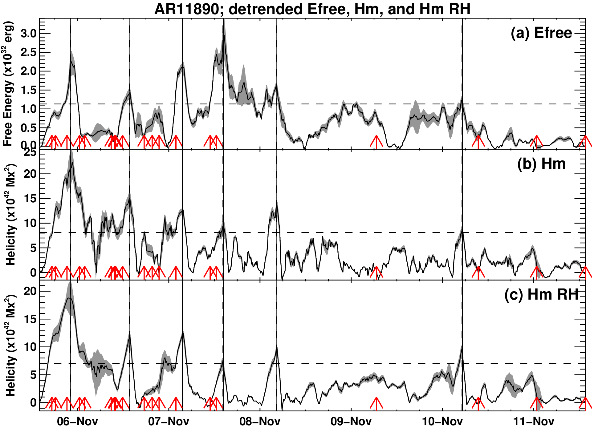
Figure 10: Detrended time series (see text for details) of the free magnetic energy (panel a), the net helicity (panel b), and the prevailing signed component of helicity (right-handed, panel c) for AR11890. The dashed lines denote the $2\sigma$ level of the quantities above the (removed) background.

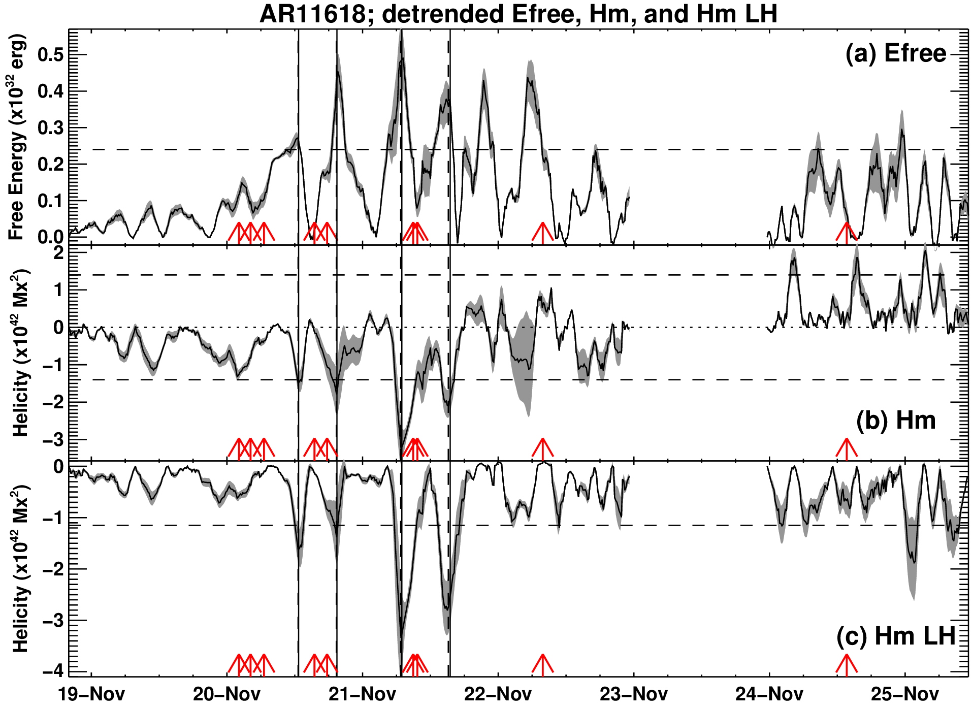
Figure 11: Same as Fig. 10 but for AR11618, with the exception that in panel (c) the left-handed helicity is displayed. The dashed lines denote the $\pm 2\sigma$ level of the quantities and the dotted line the zero helicity.

Table 2: Eruptive flares in AR11890

Event	Flare start and maximum	Flare class	$\Delta E_{f}$	$\Delta H$	$\Delta E_{f}$	$\Delta H$
Number	(UT)		($\times 10^{32}$ erg)	($\times 10^{42}$ Mx2)	(%)	(%)
1	2013 Nov. 05 22:07 22:12	X3.3	2.0	20.6	20	25
2	2013 Nov. 06 13:39 13:46	M3.8	1.1	14.9	33	62
3	2013 Nov. 07 03:34 03:40	M2.3	1.5	11.9	33	50
4	2013 Nov. 07 14:15 14:25	M2.4	1.8	8.8	35	42
5	2013 Nov. 08 04:20 04:26	X1.1	1.5	14.8	46	66
6	2013 Nov. 10 05:14 05:18	X1.1	0.8	7.6	61	48

Table 3: Eruptive flares in AR11618

Event	Flare start and maximum	Flare class	$\Delta E_{f}$	$\Delta H$	$\Delta E_{f}$	$\Delta H$
Number	(UT)		($\times 10^{32}$ erg)	($\times 10^{42}$ Mx2)	(%)	(%)
1	2012 Nov. 20 12:36 12:41	M1.7	0.28	-1.65	37	98
2	2012 Nov. 20 19:21 19:28	M1.6	0.45	-1.28	10	82
3	2012 Nov. 21 06:45 06:56	M1.4	0.41	-2.70	20	36
4	2012 Nov. 21 15:10 15:38	M3.5	0.38	-2.56	16	83

To better reveal the local peaks of free energy, net helicity, and prevailing signed component of helicity budgets (that is, right-handed for AR11890 and left-handed for AR11618) associated with the eruptive flares, we separated them from the long-term slowly varying background evolution of the respective time series. The background subtraction was done by fitting spline curves to the free energy and helicity time series that appear in Figs 3 and 4. We followed such a procedure because it was not possible to fit the slowly-varying background by using a single polynomial throughout a given time series. The resulting detrended curves appear in Figs. 10 for AR11890 and 11 for AR11618. In order to check the reliability of our background subtraction scheme we compared the values of the peaks in the detrended time series with those resulting from the following procedure. In the time series of Figs. 3 and 4 we found the inflection points just before and just after each major eruption-related local peak, calculated the corresponding average $E_{f}$, $H$ and $H_{\pm}$ value which was then subtracted from the pertinent local peak. The two methods yielded similar values for the local peaks (differences of up to about 10%).

In the detrended time series, the eruption-related changes were calculated as the difference between the pertinent local peak and the value at the inflection point just after the local peak. The results for ARs 11890 and 11618 appear in the fourth and fifth columns of Tables 2 and 3, respectively. These free energies are broadly consistent with previous results from magnetic field extrapolations (e.g. see Emslie et al., 2005, 2012; Sun et al., 2012; Tziotziou et al., 2013; Aschwanden et al., 2014; Thalmann et al., 2015) while the helicities are broadly consistent with reported helicities of magnetic clouds (e.g. see Lepping et al., 1990, 2006; DeVore, 2000; Démoulin et al., 2002; Lynch et al., 2003; Georgoulis et al., 2009; Patsourakos & Georgoulis, 2016).

Figs. 10 and 11 indicate that all eruptive events occurred at times when the free magnetic energy, net helicity, and prevailing signed component of helicity local peaks exceed the 2$\sigma$ level ($\sigma$ denotes the standard deviation) of the pertinent time series. The 2$\sigma$ levels are marked with horizontal dashed lines in Figs. 10 and 11. It is interesting that in cases where one of $E_{f}$ or $H$, but not both, exceed the 2$\sigma$ level, no eruptive activity is registered. The same conclusion holds if we replace $H$ with the prevailing signed component of helicity.

By fitting gaussians to the eruption-related components of the detrended timeseries of Figs. 10 and 11, we found that their full width at half maximum (FWHM) are in the range 3.7-8.1 hours. No essential differences were found between $E_{f}$, $H$, and prevailing signed component of $H$.

We also note that the time profiles of the normalized parameters related to the free magnetic energy, the net helicity and the prevailing signed component of helicity (see Figs. 6 and 7, and the discussion in Sect. 4.4) also show well defined local peaks associated with the major eruptive flares. In the sixth and seventh columns of Tables 2 and 3 we give the corresponding percentages of $E_{f}$ and $H$ losses (in their normalized parameters) associated with the major eruptive flares of AR11890 and 11618, respectively.

6 Summary and conclusions

Using the CB method by Georgoulis et al. (2012b), we studied the free magnetic energy and helicity in two differently evolving eruptive ARs, AR11890 and 11618. Using this calculation we were able to identify all major patterns of photospheric magnetic field evolution (see Sect. 1). However, it is clear that intense flux decay dominated the evolution of AR11890 for more than half of the observations. Flux decay was later paired with flux emergence until the end of the observations. AR11890 was the site of six major eruptive flares (three X-class and three M-class); all but the last one occurred during the flux decay phase. On the other hand the evolution of AR11618 was dominated primarily by flux emergence. This AR was the site of four eruptive M-class flares.

In both ARs, the evolution of the free magnetic energy and helicity can be understood in terms of the superposition of a slowly varying component (with characteristic time scales of more than 24 hours) and localized peaks, some of which associated with eruptive flares (the characteristic time scales of the apparently eruption-related energy and helicity changes are 3.7-8.1 hours). In both ARs the evolution of the total magnetic energy is largely consistent with the evolution of the connected magnetic flux. The same is true for the evolution of the free energy in AR11890 but not in AR11618; in the latter case the correlation worsens.

The long-term evolution of both signed components of the helicity is also consistent with the evolution of the connected flux. However, this is not the case for the net helicity because in both ARs it changes sign during the observations. It is believed (see Vemareddy & Démoulin, 2017; Vemareddy, 2021, 2022) that ARs featuring successive injection of opposite helicity do not produce CMEs. Our study shows two remarkable counter-examples; in addition to the accumulation of substantial free energy budgets, our ARs also accumulate substantial amounts of net helicity to enter them in eruptive territory despite the fact that relatively shortly thereafter (19 hours in AR11890 and 14 hours in AR11618) their helicity changes sign. This is one of the important findings of this work because (1) such reports are rare, and (2) the ARs involved featured different patterns of photospheric magnetic field evolution.

Our study was not only able to detect the change of the net helicity sign during observations but also (thanks to the properties of the CB method) to unravel, at any given time, the relative contributions of the signed components of helicity to the net helicity budget. The helicity imbalance parameter that we used in Sect. 4.3 indicates that throughout the evolution of the ARs the prevelance of a particular helicity sign is far from overwhelming; in other words, the minority helicity sense (i.e., sign) has always a significant contribution to the net helicity budget. The helicity imbalance is similar to that of quiet Sun areas which are already known to show low degrees of imbalance (Tziotziou et al., 2014, 2015). In a separate study, it would be interesting to consider the degree of compliance of such spatially incoherent distributions of the signed components of helicity with the popular scenario that a deep-seated dynamo mechanism (e.g. see Stein & Nordlund, 2012; Fan, 2021, and references therein) sometimes plays a significant role in the generation of AR magnetic flux.

The results from the CB method show moderate qualitative agreement with those from the flux-integration method, and this is to be expected given the different nature of the results provided by the two methods: instantaneous values versus accumulated changes over certain intervals, respectively (see Sect. 4.5 for more details). We note in passing that $E_{f}$ and $H$ around the time of AR11890’s major flare 5 have also been computed by Gupta et al. (2021) using a finite-volume method. The overall conclusions for their 10 flare events are different from ours (they found that $E_{f}$ and $H$ are not good proxies for the eruptive potential of the ARs) possibly due to different data and/or method they used. However, the evolutionary trends they recovered for AR11890’s major flare 5 are similar to those presented in our Fig. 8(e,f) with the important exceptions that we deduce peak $E_{f}$ and $H$ values that are about 30% and factor of 3.5, respectively, higher than theirs. The CB method is supposed to provide lower limits to the $E_{f}$ and $H$ budgets (see Sect. 3.1). However, if the NLFF field extrapolations used in the finite-volume methods converge close to a potential field, then the resulting free energy and helicity could conceivably be smaller than the ones provided by the CB method.

In both ARs all major eruptive flares occur at times of well-defined simultaneous local peaks of both the free magnetic energy and net helicity. The discrete, beyond error bars, signature of these changes may reflect significant re-organizations of the AR’s magnetic field which is supported by the distinct appearance of local peaks in the time profiles of the connected flux as well. This result can be further appreciated if we recall that (1) the instantaneous $E_{f}$ and $H$ time profiles reflect the net result of the competition between new free energy and helicity injected into the AR and their removal through flares ($E_{f}$) and CMEs (both $E_{f}$ and $H$). (2) There are several studies of major flares in which the identification of discrete decreases of either the free magnetic energy (e.g. Metcalf et al., 2005) or the helicity (e.g. Patsourakos et al., 2016) as a result of the flare was not possible beyond uncertainties.

The occurrence of simultaneous local free magnetic energy and helicity peaks during the impulsive phase of the flares is consistent with a paradigm which dictates that (1) the prior accumulation of sufficient amounts of free magnetic energy and helicity is a necessary condition for an AR to erupt, and (2) in the course of the eruption free energy is released and helicity is bodily removed from the AR resulting in the decrease of the budgets of both quantities just after the eruption. Furthermore, it is in line with those results that advocate for a synchronization between the CME acceleration and the impulsive phase of the flare.

The occurrence of all major flares at times when the ARs contained significant budgets of both signed components of helicity may appear in favor of the helicity annihilation mechanism for the onset of solar flares (Kusano et al., 2003, 2004). However, we note that in most cases the major flares in our ARs occurred around times that the minority helicity sense showed small temporal changes.

The results from the computation of the free magnetic energy and net helicity changes associated with the eruptive events appear in Tables 2 and 3; the free magnetic energy and net helicity losses ranged from $(0.3-2)\times 10^{32}$ erg and $(1.3-20\times 10^{42}$ Mx², respectively (their average values being $1.02\times 10^{32}$ erg and $8.68\times 10^{42}$ Mx², respectively). These values are broadly consistent with results from previous publications. The percentage losses, associated with the eruptive flares, in the normalized free magnetic energy were significant, in the range $\sim$10-60%. For the magnetic helicity, changes ranged from $\sim$25% to the removal of the entire excess helicity of the prevailing sign, leading a roughly zero net helicity. Such extremely high helicity percentage losses do not really mean that the active region has turned to potentiality (this would be implied if the entire free energy was wiped out, as well, but this is not the case). It simply implies that the AR gives out the entire excess helicity of one sign and turns to a situation of almost zero net helicity, with very significant, but roughly equal and opposite, budgets of both signs.

Another new result is that we were able to identify the occurrence of the eruptive flares at those times when both the free magnetic energy and the net helicity as well as the prevailining signed component of helicity local peaks exceed the 2$\sigma$ level of their detrended timeseries. Furthermore, there is no eruption when none of these quantities or only the free magnetic energy or only the helicities exceeds its 2$\sigma$ level. These results place free energy and helicity on an equal footing as far as their role in the initiation of eruptive events. Given that both ARs possess adequate free energy and helicity budgets (that is, higher than those released in a typical eruption) throughout much of their evolution, this result may plausibly explain the eruption timing. Clearly, studies of more ARs are required in order to test whether this threshold represents a universal property of eruptive ARs or is peculiar to the ARs studied in this paper.

The above result can be reproduced in AR11890 if we use the normalized parameters, $E_{f}/E_{tot}$, and $H/\Phi_{conn}^{2}$ or $H_{+}/\Phi_{conn}^{2}$ (see Sect. 4.4) instead of $E_{f}$ and $H$ or $H_{+}$. However, this is not the case for AR11618 because its $E_{f}/E_{tot}$ curve shows two pronounced peaks on November 19 which are not associated with eruptions and also its local peak at the time of the second major flare is small (see Fig. 7). Therefore the overall potential of this particular set of normalized parameters as indicators of the AR approach to eruption territory is rather weaker than that of $E_{f}$ and $H$. Having said that, the large percentage losses, associated with the eruptive flares, in the normalized free magnetic energy and helicity parameters (see Figs 6 and 7 as well as Tables 2 and 3) is a particularly notable feature, rarely seen in such clarity.

Both the CB and the finite-volume methods cannot provide any density for helicity and therefore a detailed picture of the spatial distribution of instantaneous helicity is largely unknown. A way to bypass this obstacle is by employing the concept of relative field line helicity (e.g. Yeates & Page, 2018; Moraitis et al., 2019). Although this is a gauge-dependent quantity, its first application to solar data (Moraitis et al., 2021) shows that its morphology is not sensitive on the gauge used in its computation, and therefore becomes a promising proxy for the recovery of the density of helicity in conjunction with the locations of major flare activity. A computation of the evolution of the field line helicity in the ARs studied here should be an obvious extension of this work.