Even- and odd-orthogonality properties of the Wigner D-matrix and their metrological applications

Abstract

The Wigner D-matrix is essential in the course of angular momentum techniques. We here derive the new even- and odd-orthogonality properties of the Wigner D-matrix which was yet to be demonstrated in textbooks and also apply them to identifying optimal measurements for linear phase estimation based on two-mode optical interferometry with two specific quantum states.

1 Introduction

The quantum theory of angular momentum, as developed principally by Eugene Wigner Wigner1967Book , has become an indispensable discipline for quantitative study of problems in atomic physics, molecular physics, nuclear physics and solid state physics Biedenhar1984Book . Angular momentum theory is of greater importance in the theory of atomic and molecular physics and other quantum problems involving rotational symmetry. It is naturally applied to represent the physical state of a quantum system, due to the inherent connection between the properties of elementary particles to the structure of Lie group and Lie algebra. Angular momentum operators are defined as the generators of SU(2) and SO(3) groups, which consists of a mathematical structure of a Lie algebra.

To quantitatively represent a state of quantum system of $N$ qubits, the routine means is to use the collective angular momentum operators $J_{\xi}=\sum_{{}_{i=1}}^{N}\sigma_{i\xi}/2$ $\left(\xi=x,y,z\right)$ with $\sigma_{i\xi}$ the Pauli matrix of the $i$th qubit, satisfying the following commutation relations $\left[J_{i},J_{j}\right]=i\epsilon_{ijk}J_{k}$$\ \left(i,j,k=\left\{x,y,z\right\}\right)$ with $\epsilon_{ijk}$ the Levi-Civita symbol. The basis space is spanned by the common eigenstates $|j,m\rangle$ of the operators $J^{2}=J_{x}^{2}+J_{y}^{2}+J_{z}^{2}$ and $J_{z}$ with the eigenvalues $j\left(j+1\right)$ and $m=-j,-j+1,\ldots,j$, respectively, where the quantum number $j$ in the spherical basis $|j,m\rangle$ is given by $j=0,1/2,1,3/2,2,\ldots$ for SU(2), and $j=0,1,2,\ldots$ for SO(3). A general $3$-dimensional rotation operator can be conveniently described in terms of the three Euler angles $\alpha$, $\beta$ and $\gamma$ $\left(0<\alpha<2\pi,0<\beta<\pi,0<\gamma<2\pi\right)$ as

$$R\left(\alpha,\beta,\gamma\right) \equiv e^{-i\alpha J_{z}}e^{-i\beta J_{y}}e^{-i\gamma J_{z}},$$ (1)

In the basis of $\left\{|j,m\rangle\right\}$, the rotation operator $R$ can be represented as a square matrix of dimension $2j+1$ with general element

$$D_{m^{\prime}\!,m}^{j}\!\left(\alpha,\beta,\gamma\right) \!=\! \langle j,m^{\prime}|R\left(\alpha,\beta,\gamma\right)|j,m\rangle\!=\!e^{-im^{\prime}\!\alpha}d_{m^{\prime}\!,m}^{j}\!\left(\beta\right)e^{-im\gamma},\quad$$ (2)

which is the so-called Wigner D-matrix introduced in 1927 by Eugene P. Wigner. The Wigner D-matrix is a matrix in an irreducible representation of the groups SU(2) and SO(3). In above, the matrix with general element

$$d_{m^{\prime},m}^{j}\left(\beta\right) \equiv \langle j,m^{\prime}|e^{-i\beta J_{y}}|j,m\rangle,$$ (3)

is known as the Wigner (small) $d$-matrix Wigner1959Book . Apparently, the Wigner D-matrix reduces to the Wigner (small) $d$-matrix when we let $\alpha=\gamma=0$.

Wigner rotation matrix has been proposed for over a century and its relevant properties are almost comprehensively written into textbooks Wigner1959Book ; Biedenhar1984Book , for instance, the orthogonality relation of the Wigner D-matrix

$$\sum_{\mu=-j}^{j}D_{m^{\prime},\mu}^{j}\left(\alpha,\beta,\gamma\right)D_{m,\mu}^{j}\left(\alpha,\beta,\gamma\right)^{\ast} = \delta_{m^{\prime},m}.$$ (4)

In this paper, we introduce two new orthogonality relations of the Wigner D-matrix which was yet to be demonstrated in textbooks. We first present a brief derivation of them by simply specifying a quantum state $|\psi\rangle$ in an ansatz space associating with zero-value expectation of $J_{z}$ for $|\psi\rangle$, i.e., $\langle J_{z}\rangle_{\psi}=0$. We then apply these orthogonality relations to two-mode optical interferometry to identify optimal measurements to access the ultimate sensitivity of phase estimation with two specific states.

This paper is organized as follows. In Sect. 2, we first explicitly derive the two new orthogonality relations of the Wigner D-matrix. In. Sect. 3, we invoke these relations to identify the optimal measurements for Mach-Zehnder interferometry with NOON and entangled coherent states. Finally, the conclusions are given in Sect. 4.

2 Even- and odd-orthogonality properties of the Wigner D-matrix

We first present the two novel even- and odd-orthogonality properties in terms of the Wigner D-matrix that we would like to derive in the following. For odd $N$, we have the following identities

$$\sum_{k=\left\{{\rm even,odd}\right\}}D_{j-k,m}^{j}\left(\alpha,\frac{\pi}{2},\gamma\right)D_{j-k,m^{\prime}}^{j}\left(\alpha,\frac{\pi}{2},\gamma\right)^{\ast} = \frac{1}{2}\delta_{m,m^{\prime}},$$ (5)

where $k$ runs over the even or odd numbers from $0$ to $N$. As such, we call the above relations as even- and odd-orthogonality properties of the Wigner D-matrix. The above identities also hold for even $N$ when $m\neq 0$, but when $m=0$ they become

$$\sum_{k={\rm\left\{even,odd\right\}}}D_{j-k,0}^{j}\left(\alpha,\frac{\pi}{2},\gamma\right)D_{j-k,m^{\prime}}^{j}\left(\alpha,\frac{\pi}{2},\gamma\right)^{\ast} = \delta_{0,m^{\prime}},$$ (6)

up to absence of a fact of $1/2$. Obviously, Eqs. (5) and (6) are different from Eq. (4), since one can obtain Eq. (4) with $\beta=\pi/2$ by summarizing Eqs. (5) and (6), while the opposite is not possible. The above expressions can be simplified to a form where the conjugation operation can be removed for $\alpha=\gamma=0$ since the resulting $d$-matrix elements as $D_{m^{\prime}\!,m}^{j}\!\left(0,\beta,0\right)=d_{m^{\prime}\!,m}^{j}\!\left(\beta\right)$ are real.

To derive the above identities, we first recall the orthogonality property of the Wigner D-matrix given by Eq. (4) which can be directly derived from the fact that the normalization condition of a quantum state $|\psi\rangle$ is still sustained after a rotation operation $R\left(\alpha,\beta,\gamma\right)$, suggesting that $\langle\psi|R^{\dagger}\left(\alpha,\beta,\gamma\right)R\left(\alpha,\beta,\gamma\right)|\psi\rangle=\langle\psi|\psi\rangle=1$ due to $R^{\dagger}R=\bm{1}$. Assume the total number of qubits of the system is fixed as $N$, thus identifying $j=N/2$. Thus a generic pure state can be expanded in terms of the basis of $\left\{|j,m\rangle\right\}$ as $|\psi\rangle=\sum_{m}C_{m}|j,m\rangle$, associating with $\sum_{m}\left|C_{m}\right|^{2}=1$. We denote the state after the rotation operation $R\left(\alpha,\beta,\gamma\right)$ by $|\tilde{\psi}\rangle\equiv R\left(\alpha,\beta,\gamma\right)|\psi\rangle$. It can also be expanded as $|\tilde{\psi}\rangle=\sum_{\mu}\tilde{C}_{\mu}|j,\mu\rangle$ where the expanded coefficients is given by $\tilde{C}_{\mu}\equiv\sum_{m}D_{\mu,m}^{j}\left(\alpha,\beta,\gamma\right)C_{m}$, satisfying the normalization condition $\sum_{\mu}|\tilde{C}_{\mu}|^{2}=1$. With the normalization $\sum_{\mu}|\tilde{C}_{\mu}|^{2}=\sum_{m}|C_{m}|^{2}=1$, the orthogonality relation of Eq. (4) can be obtained.

The procedure used in above can be straightforwardly extended to derive Eqs. (5) and (6). Here we make two restrictions. First, the pure state $|\psi\rangle$ is assumed to be in an ansatz subspace satisfying $C_{m}=C_{-m}$, implying that $\langle J_{z}\rangle_{\psi}=0$, which encompasses an amount of quantum states implemented in experiments Caves1981PRD ; Campos2003PRA ; Pezze2008PRL ; Huver2008PRA ; Hofmann2009PRA ; Lucke2011Science ; Anisimov2010PRL ; Liu2013PRA ; Pezze2013PRL ; Froewis2014NJP ; Zhong2017PRA ; Zhong2020SC ; Zhong2021PRA ; Lang2013PRL . Note that this restriction we assume here is simply convenient for our derivation, but the final result does not depend on what type of quantum state is used. Second, the rotation angle $\beta$ is specified by $\beta=\pi/2$, giving $R\left(\alpha,\pi/2,\gamma\right)$. This is a very reasonable assumption. If let $\alpha=\gamma=0$, thus the rotation operation is $R_{y}\left(\pi/2\right)\equiv R\left(0,\pi/2,0\right)$, which can be implemented to characterize a class of quantum coherent operations, such as a balanced beam splitter in linear optical system or a $\pi/2$-pulse in atomic system. Under these constraints, the expansion coefficients for the state after the rotation is given by

$$\tilde{C}_{\mu} = \sum_{m=-j}^{j}\!C_{m}\,D_{\mu,m}^{j}\!\left(\alpha,\frac{\pi}{2},\gamma\right).$$ (7)

With the help of $C_{m}=C_{-m}$, it can be expressed as the following form

$$\tilde{C}_{\mu} = \begin{cases}\sum\limits_{m=1/2}^{j}C_{m}\left[D_{\mu,-m}^{j}\left(\alpha,\frac{\pi}{2},\gamma\right)+D_{\mu,m}^{j}\left(\alpha,\frac{\pi}{2},\gamma\right)\right],&\text{for odd }N,\\ \sum\limits_{m=1}^{j}C_{m}\left[D_{\mu,-m}^{j}\left(\alpha,\frac{\pi}{2},\gamma\right)+D_{\mu,m}^{j}\left(\alpha,\frac{\pi}{2},\gamma\right)\right]+C_{0}D_{\mu,0}^{j}\left(\alpha,\frac{\pi}{2},\gamma\right),&\text{for even }N.\end{cases}$$ (8)

By employing the identity $D_{\mu,-m}^{j}\left(\alpha,\frac{\pi}{2},\gamma\right)=\left(-1\right)^{-j-\mu}D_{\mu,m}^{j}\left(\alpha,\frac{\pi}{2},\gamma\right)$ Wigner1967Book ; Biedenhar1984Book , the above expression can be further represented as

$$\tilde{C}_{\mu} = \begin{cases}\sum\limits_{m=1/2}^{j}C_{m}\left[1+\left(-1\right)^{-j-\mu}\right]D_{\mu,m}^{j}\left(\alpha,\frac{\pi}{2},\gamma\right),&\text{for odd }N,\\ \sum\limits_{m=1}^{j}C_{m}\left[1+\left(-1\right)^{-j-\mu}\right]D_{\mu,m}^{j}\left(\alpha,\frac{\pi}{2},\gamma\right)+C_{0}D_{\mu,0}^{j}\left(\alpha,\frac{\pi}{2},\gamma\right),&\text{for even }N.\end{cases}$$ (9)

For simplicity, we below take the case of odd $N$ for example. With Eq. (9) and by setting $k\equiv j+\mu$, we have

$$\sum_{\mu=-j}^{j}\left|\tilde{C}_{\mu}\right|^{2} = \sum_{m,m^{\prime}=1/2}^{j}2C_{m}C_{m^{\prime}}^{\ast}\left\{\sum_{k=0}^{N}\left[1+\left(-1\right)^{-k}\right]D_{j-k,m}^{j}\left(\alpha,\frac{\pi}{2},\gamma\right)D_{j-k,m^{\prime}}^{j}\left(\alpha,\frac{\pi}{2},\gamma\right)^{\ast}\right\}$$ (10)

$$= \sum_{m,m^{\prime}=1/2}^{j}2C_{m}C_{m^{\prime}}^{\ast}\times\left[2\sum_{k={\rm even}}D_{j-k,m}^{j}\left(\alpha,\frac{\pi}{2},\gamma\right)D_{j-k,m^{\prime}}^{j}\left(\alpha,\frac{\pi}{2},\gamma\right)^{\ast}\right].$$

Obviously it suggests the relation of Eq. (5) with $k=$ even numbers from $0$ to $N$ must be satisfied due to the normalization $\sum_{\mu=-j}^{j}|\tilde{C}_{\mu}|^{2}=\sum_{m=-j}^{j}\left|C_{m}\right|^{2}=\sum_{m=1/2}^{j}\!2\left|C_{m}\right|^{2}=1$. Thus the relation of Eq. (5) with $k=$ odd numbers from $0$ to $N$ can be obtained by taking the difference between Eq. (4) with $\beta=\pi/2$ and Eq. (5). Similarly, the derivation for the case of even $N$ just follows the same procedure used in above derivation, but minding the term of $m=0$, which needs to be treated solely in the square sum calculation.

3 Optimal measurements for linear phase estimation

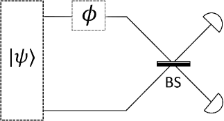
Figure 1: (Color online) Schematic of linear phase estimation based on two-mode optical interferometry.

To view the effectiveness of even- and odd-orthogonality properties obtained above, we apply them into the linear phase estimation problem to identify optimal measurement for saturating the ultimate sensitivity limit in Mach-Zehnder interformetry with different probe states. A generic MZI is composed of two balanced beam splitters $B_{i}$ $(i=1,2)$ and a phase shifting $U_{\phi}$ with $\phi$ to be estimated. Here we identify the state after the first beam splitter $B_{1}$ as the probe state $\rho\equiv B_{1}\rho_{{\rm in}}B_{1}^{\dagger}$ with $\rho_{{\rm in}}$ the input state injecting at the input port of the interferometer (see Fig. 1). Under $U_{\phi}$, the probe state evolves into a parametric state as $\rho\left(\phi\right)=U_{\phi}\rho U_{\phi}$. Finally, a measurement is performed at the output port of the interferometer where the output state reads $\rho_{{\rm out}}\left(\phi\right)=B_{2}\rho\left(\phi\right)B_{2}^{\dagger}$, and then the true value of the phase shift is inferred from the measurement outcomes.

Consider a general measurement described by a positive-valued measure $\bm{M}=\left\{M_{\chi}\right\}$, with $\chi$ the results of measurement. Based on $\bm{M}$, the sensitivity of an unbiased phase estimator $\phi_{{\rm est}}$ is limited by the classical Cramér-Rao bound $\Delta^{2}\phi_{{\rm est}}\geq\left[\upsilon F\left(\rho_{{\rm out}}\left(\phi\right)|\bm{M}\right)\right]^{-1}$, where $\upsilon$ is the repetitions of the experiments and $F$ is the classical Fisher information (CFI) defined by Helstrom1976Book ; Holevo1982Book

$$F=\sum_{\chi}\frac{1}{p\left(\chi|\rho_{{\rm out}}\left(\phi\right)\right)}\left[\frac{\partial p\left(\chi|\rho_{{\rm out}}\left(\phi\right)\right)}{\partial\phi}\right]^{2},$$ (11)

with $p\left(\chi|\rho_{{\rm out}}\left(\phi\right)\right)={\rm Tr}\left(M_{\chi}\rho_{{\rm out}}\left(\phi\right)\right)$ the probability of the outcome $\chi$ conditioned on the specific value of $\phi$ contained in $\rho_{{\rm out}}\left(\phi\right)$. It is well known that such an accessible sensitivity bound is achieved by the maximum likelihood estimator for sufficiently large $\upsilon$ with Bayesian estimation methods Krischek2011PRL ; Olivares2009JPB ; Uys2007PRA . A quantum analog of Cramér-Rao bound is identified by optimizing the measurements over the positive-valued measure operators $\bm{M}$, such that $\Delta\phi_{{\rm est}}\geq\left(\upsilon H\right)^{-1}$ with $H=\sup_{\bm{M}}\left(F\right)$ denoting the quantum Fisher information (QFI) Braunstein1994PRL ; Lu2012PRA . For pure states $\rho\left(\phi\right)=|\psi\left(\phi\right)\rangle\langle\psi\left(\phi\right)|$ with $|\psi\left(\phi\right)\rangle=U_{\phi}|\psi\rangle$, the QFI can be explicitly expressed as

$$H=4\left(\langle\partial_{\phi}\psi\left(\phi\right)|\partial_{\phi}\psi\left(\phi\right)\rangle-\left|\langle\psi\left(\phi\right)|\partial_{\phi}\psi\left(\phi\right)\rangle\right|^{2}\right),$$ (12)

with $\partial_{\phi}\psi\left(\phi\right)\equiv\partial\psi\left(\phi\right)/\partial\phi$ being the derivative of $\psi\left(\phi\right)$ with respect to $\phi$. If we assume that the phase parameter $\phi$ here is imprinted via a unitary operation $U_{\phi}=\exp\left(-iG\phi\right)$ with $G$ the generator, then the expression of Eq. (12) can be simplified as four times the variance of the generator $G$ for the pure state $|\psi\rangle$, equivalently

$$H=4\left\langle\Delta^{2}G\right\rangle_{\psi}=4\big{(}\left\langle G^{2}\right\rangle_{\psi}-\left\langle G\right\rangle_{\psi}^{2}\big{)}.$$ (13)

Note that, in the setting as mentioned above, the QFIs for the states before and after the second beams splitter are identical due to the invariance property of the QFI under a phase-independent unitary evolution Helstrom1976Book ; Holevo1982Book . We below take the CFI and QFI as the two figure of merits, as they are widely used to evaluate the performance of various metrological applications Ozaydin2015SR ; Ozaydin2020OQE ; Wang2020Met ; Zhong2013PRA ; Cai2020QIP ; Guo2022PRA ; Zhong2020SC ; Zhong2017PRA ; Zhong2014CPB ; Taylor2016PR ; Pezze2018RMP ; Polino2020review ; Sparaciari2015JOSAB ; Sparaciari2016PRA . Hence, an efficient way to identify a measurement being optimal for a quantum phase estimation task is to test whether the QFI and the CFI with respect to a specific measurement are identical Braunstein1994PRL ; Zhong2014JPA .

In what follows, the probe states of interest here are restricted to NOON Rarity1990PRL ; Lee2002JOP and entangled coherent (EC) states Joo2011PRL (see below for definitions). The measurement of interest here is a double-photon-counting (DPC) detection, which can be represented as the projection operator $M=\left\{|n_{a},n_{b}\rangle\langle n_{a},n_{b}|\right\}$ Pezze2008PRL ; Pezze2013PRL ; Lang2013PRL ; Zhong2017PRA with the pairs of outcomes ($n_{a},n_{b}$) recording the photon numbers detected at the two output ports of the interferometer. Thus, to implement this measurement, a high-efficiency photon-number-resolving detector is demanded in experiments Divochiy2008NP ; Sahin2013APL .

3.1 NOON states

Let us first consider the NOON state as the probe state, which can be expressed as $\left|N::0\right\rangle=\left(|N0\rangle+|0N\rangle\right)/\sqrt{2}$ with $|N0\rangle$ $\left(|0N\rangle\right)$ denoting the $N$ photons (null) in mode $a$ and null ($N$ photons) in mode $b$, respectively. The operation of phase shifting is assumed to be expressed as $U\left(\phi\right)=\exp\left(-ia^{\dagger}a\phi\right)$, where $a^{\dagger}\left(a\right)$ stands for the creation (annihilation) operator of the corresponding mode. Hence, the NOON state under $U\left(\phi\right)$ evolves into a parametric one $\left|N::0,\phi\right\rangle\equiv U\left(\phi\right)|N::0\rangle$. Such a strategy is expected to be possibly achieving a Heisenberg-scaling sensitivity $\Delta\phi\sim N^{-1}$ Rarity1990PRL ; Lee2002JOP , that is $H_{{\rm NOON}}=N^{2}$ Zhong2021PRA .

To access this limit, we consider the DPC measurement. The probability of detecting the photon numbers $\left(n_{a},n_{b}\right)$ at the two-output ports is given by

$$p\left(n_{a},n_{b}|N::0,\phi\right)=\left|\langle n_{a},n_{b}|R_{y}\left(\frac{\pi}{2}\right)\left|N::0,\phi\right\rangle\right|^{2},$$ (14)

where we have assumed the operation of the second BS to be $B_{2}=R_{y}\left(\pi/2\right)$ following the form commonly adopted in previous works Zhong2017PRA ; Zhong2020SC ; Zhong2021PRA ; Guo2022PRA . For simplicity, we use the angular momentum technique (which is also called Schwinger representation Yurke1986PRA ) to represent the two-mode optical interferometry by defining $J_{x}=\left(a^{\dagger}b+ab^{\dagger}\right)/2$, $J_{y}=\left(a^{\dagger}b-ab^{\dagger}\right)/2i$ and $J_{z}=\left(a^{\dagger}a-b^{\dagger}b\right)/2$. Thus the NOON state can be rewritten by $\left|N::0\right\rangle=\left(|j,j\rangle+|j,-j\rangle\right)/\sqrt{2}$ with $j=N/2$, correspondingly, the parametric NOON state reads $\left|N::0,\phi\right\rangle=\left(e^{-ij\phi}|j,j\rangle+e^{ij\phi}|j,-j\rangle\right)/\sqrt{2}$. Identifying $j^{\prime}=\left(n_{a}+n_{b}\right)/2\text{ and }m^{\prime}=\left(n_{a}-n_{b}\right)/2$, one can obtain $p\left(n_{a},n_{b}|N::0,\phi\right)=p\left(j^{\prime},m^{\prime}|N::0,\phi\right)$. Note that the irreducible representation of angular momentum requires the two states spanned in different irreducible subspaces are orthogonal in the sense that we have $j^{\prime}=j=N/2$. Hence, by setting $j-m^{\prime}\equiv k$, the above expression can be further expressed as

$$p\left(j,j-k|N::0,\phi\right) = \begin{cases}\left[d_{j-k,j}^{j}\left(\frac{\pi}{2}\right)\right]^{2}2\cos^{2}\left(j\phi\right),&\text{even }k,\\ \left[d_{j-k,j}^{j}\left(\frac{\pi}{2}\right)\right]^{2}2\sin^{2}\left(j\phi\right),&\text{odd }k.\end{cases}$$ (15)

Submitting the above results into the definition of the CFI finally yields

$$F_{{\rm NOON}} = \sum_{n_{a},n_{b}}\frac{1}{p\left(n_{a},n_{b}|N::0,\phi\right)}\left[\frac{\partial p\left(n_{a},n_{b}|N::0,\phi\right)}{\partial\phi}\right]^{2}$$ (16)

$$= \sum_{k}\frac{1}{p\left(j,j-k|N::0,\phi\right)}\left[\frac{\partial p\left(j,j-k|N::0,\phi\right)}{\partial\phi}\right]^{2}$$

$$= \sum_{k={\rm even}}\left[d_{j-k,j}^{j}\left(\frac{\pi}{2}\right)\right]^{2}8j^{2}\sin^{2}\left(j\phi\right)+\sum_{k={\rm odd}}\left[d_{j-k,j}^{j}\left(\frac{\pi}{2}\right)\right]^{2}8j^{2}\cos^{2}\left(j\phi\right)$$

$$= N^{2},$$

where the last equality is obtained by employing the even- and odd-orthogonality properties in terms of the Wigner $d$-matrix obtained from Eq. (5) by setting $\alpha=\gamma=0$. Obviously, we find that $F_{{\rm NOON}}=H_{{\rm NOON}}$, in the sense that the DPC detection is an optimal measurement for saturating the Heisenberg limit expected by NOON states. Moreover, it is also shown that the result of $F_{C,{\rm NOON}}$ is $\phi$-independent, suggesting that the DPC detection is globally optimal over the full range of phase shift values.

More importantly, from Eq. (15), it is shown that the probability of detection only depends on a single variable $k$ (or equivalently $m^{\prime}$ due to the restriction of $N/2-m^{\prime}\equiv k$), since the states over the whole evolution process are only confined in the $j=N/2$ irreducible subspace. This means that a population difference detection (i.e., measuring $J_{z}$) at the output ports is sufficient for attaining the Heisenberg limit. Besides it also has been demonstrated that parity detection exhibits an equivalent performance as the DPC detection and population difference detection (see also Appendix for a demonstration) Seshadreesan2013PRA ; Zhong2014JPA .

3.2 Entangled coherent states

Below, we consider the EC state as the probe state, which can be understood as a superposition of NOON states with different photons,

$$|{\rm EC}\rangle = \mathcal{N}_{\alpha}\left[|\alpha\rangle|0\rangle+|0\rangle|\alpha\rangle\right]=\sqrt{2}\mathcal{N}_{\alpha}\sum_{n=0}^{\infty}c_{n}|n::0\rangle,$$ (17)

with $\mathcal{N}_{\alpha}=1/\sqrt{2\left(1+e^{-\left|\alpha\right|^{2}}\right)}$ the normalization factor and $c_{n}=e^{-|\alpha|^{2}/2}\alpha^{n}/\sqrt{n!}$ the superposition coefficient of the coherent state. This state can be generated by powering a coherent state into one input port mode of a beam splitter and a coherent superposition of macroscopically distinct coherent states into another input port Luis2001PRA . Note that a phase-averaging operation is required here in calculation of the QFI due to the lack of an external reference beam in out setting Jarzyna2012PRA . Under the phase-averaging operation, the EC states becomes a mixed state that consists of a statistical ensemble of NOON states, that is,

$$\rho_{{\rm EC}} = 2\mathcal{N}_{\alpha}^{2}\bigoplus_{n=0}^{\infty}\left|c_{n}\right|^{2}\left|n::0\right\rangle\left\langle n::0\right|.$$ (18)

We thus explicitly derive the QFI of the EC state as

$$H_{{\rm EC}} = 2\mathcal{N}_{\alpha}^{2}\sum_{n=1}^{\infty}\left|c_{n}\right|^{2}H_{{\rm noon}}=2\mathcal{N}_{\alpha}^{2}\sum_{n=1}^{\infty}\left|c_{n}\right|^{2}n^{2},$$ (19)

as a result of the summability of the QFI Helstrom1976Book ; Fujiwara2001PRA and $H_{{\rm NOON}}=N^{2}$. For larger amplitude $\left|\alpha\right|\gg 1$, the expression of Eq. (19) approximately reduced to $H_{{\rm EC}}=\bar{N}+\bar{N}^{2}$ with the mean photon number $\bar{N}=\left|\alpha\right|^{2}$. In contrast, it has been observed that a larger amount of $H_{{\rm EC}}^{J}=2\bar{N}+\bar{N}^{2}$ can be obtained when a common reference beam is involved Joo2011PRL . This indicates that higher estimation sensitivity could be attained when the extra reference beam is established in current setting.

Now let us identify the CFI with the DPC detection for the EC probe state. When powering EC states as the probe state, the probability of detecting $n_{a}$ and $n_{b}$ at the output ports is given by

$$p\left(n_{a},n_{b}|{\rm EC},\phi\right) = \left|\langle n_{a},n_{b}|R_{y}\left(\frac{\pi}{2}\right)\left|{\rm EC},\phi\right\rangle\right|^{2}$$ (20)

$$= 2\mathcal{N}_{\alpha}^{2}\sum_{n=0}^{\infty}\left|c_{n}\right|^{2}\left|\langle n_{a},n_{b}|R_{y}\left(\frac{\pi}{2}\right)\left|n::0,\phi\right\rangle\right|^{2}$$

$$= 2\mathcal{N}_{\alpha}^{2}\sum_{n=1}^{\infty}\left|c_{n}\right|^{2}p\left(n_{a},n_{b}|n::0,\phi\right)+4\mathcal{N}_{\alpha}^{2}\left|c_{0}\right|^{2},$$

where $\left|{\rm EC},\phi\right\rangle$ corresponds to the parametric EC state defined by $\left|{\rm EC},\phi\right\rangle=U\left(\phi\right)|{\rm EC}\rangle$ and in the last equality the second term is obtained by adopting Eq. (15) incorporating with $d_{0,0}^{0}\left(\pi/2\right)=1$. With Eq. (20) and transferring into the Schwinger representation, the CFI with the DPC detection can be derived as follows

$$F_{{\rm EC}} = \sum_{n_{a},n_{b}}\frac{1}{p\left(n_{a},n_{b}|{\rm EC},\phi\right)}\left[\frac{\partial p\left(n_{a},n_{b}|{\rm EC},\phi\right)}{\partial\phi}\right]^{2}$$ (21)

$$= \sum_{j\neq 0}\sum_{\mu=-j}^{j}\frac{\left[2\mathcal{N}_{\alpha}^{2}\sum_{n=1}^{\infty}\left|c_{n}\right|^{2}\partial_{\phi}p\left(j,\mu|n::0,\phi\right)\delta_{j,n/2}\right]^{2}}{2\mathcal{N}_{\alpha}^{2}\sum_{n=1}^{\infty}\left|c_{n}\right|^{2}p\left(j,\mu|n::0,\phi\right)\delta_{j,n/2}}$$

$$= \sum_{n=1}^{\infty}2\mathcal{N}_{\alpha}^{2}\left|c_{n}\right|^{2}\left[\sum_{\mu=-n/2}^{n/2}\frac{\left[\partial_{\phi}p\left(\frac{n}{2},\mu|n::0,\phi\right)\right]^{2}}{p\left(\frac{n}{2},\mu|n::0,\phi\right)}\right]$$

$$= 2\mathcal{N}_{\alpha}^{2}\sum_{n=1}^{\infty}\left|c_{n}\right|^{2}n^{2},$$

where we have introduced the simplified symbol $\partial/\partial\phi\equiv\partial_{\phi}$ and in the last equality we have used the result given by Eq. (16). It is remarkable that the $F_{{\rm EC}}$ is exactly equivalent to the $F_{{\rm EC}}$ and also $\phi$-independent. Obviously, the results given by Eqs. (19) and (21) are equal, which indicates that the DPC detection is also globally optimal for EC states, meanwhile it has the same role as in the case of NOON states.

In order to compare with the result obtained in Ref. Joo2011PRL but neglecting the effect of photon losses, we revisit the above phase estimation problem by taking account of parity detection as Joo et al. done Joo2011PRL . We analytically derive the CFI with parity detection as follows (see Appendix for detailed derivation)

$$F_{{\rm EC}} = \frac{\left|2\mathcal{N}_{\alpha}^{2}\sum_{n=1}^{\infty}\left|c_{n}\right|^{2}n\sin\left(n\phi\right)\right|^{2}}{1-\left(2\mathcal{N}_{\alpha}^{2}\left[2\left|c_{0}\right|^{2}+\sum_{n=1}^{\infty}\left|c_{n}\right|^{2}\cos\left(n\phi\right)\right]\right)^{2}}.$$ (22)

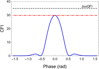
Figure 2: (Color online) The CFIs with DPC and parity measurements versus $\phi$ for the EC state with $\alpha=\sqrt{5}$. The blue curve corresponds to the parity detection and the red dot-dashed line to the DPC measurement. The black dashed line is given by $H_{\rm{EC}}^{J}=4\big{[}\mathcal{N}_{\alpha}^{2}\left(|\alpha|^{4}+|\alpha|^{2}\right)-\left(\mathcal{N}_{\alpha}^{2}|\alpha|^{2}\right)^{2}\big{]}$ derived by Joo et al. in Ref. Joo2011PRL .

It is explicitly simplified to $F_{{\rm EC}}=H_{{\rm EC}}$ in the asymptotic limit $\phi\rightarrow 0$, in the sense that the parity detection is responsible of saturating its quantum analog $H_{{\rm EC}}$ given by Eq. (19) only for small $\phi$. To view this more clearly we plot in Fig. 2 the CFIs with both DPC and parity measurements as a function of $\phi$ for EC states according to Eqs. (21) and (22). It can been seen that the value of the CFI with parity detection is lower than that with PDC detection over the whole phase interval except at the zero-point location, where they have merged satisfactorily. Such a superiority of the PDC over parity can be intuitively understood as parity results may be obtained from photon-counting results by throwing away some information, while the opposite is not possible. Thus this leads to the fact that the phase information contained in the quantum state cannot be fully extracted by the parity measurement in contrast to the PDC measurement under certain circumstances. It is shown in Fig. 2 that the sensitivity given by Joo et al. Joo2011PRL does not accessible with both the PDC and parity measurements, in contrast, ours are accessible. We identify the reason underlying this difference in the following subsection.

3.3 Further discussion

In above, we have assumed the phase shifting only acting on the single arm of the interferometer (see Fig. 1), the same as the phase configuration considered in Ref. Joo2011PRL . But the usual way to schematize a two-mode phase estimation scheme involves the phase shifts of $\phi/2$ and $-\phi/2$ in the two arms, instead of the single-phase shift $\phi$ in one arm. Let us further compare the influence of the two-phase configurations on the phase sensitivity. As assumed above, the single-phase shifting operation is modeled by $U_{1}\left(\phi\right)=\exp\left(-ia^{\dagger}a\phi\right)$, where we affix a subscript ’1’ to avoid confusion with the two-phase shifting operation expressed by $U_{2}\left(\phi\right)=\exp\left[-i\left(a^{\dagger}a-b^{\dagger}b\right)\phi/2\right].$ By resorting to the Schwinger representation, the above two operations can be reformulated as

$$U_{1}\left(\phi\right)=\exp\Big{[}-i\Big{(}\frac{\hat{N}}{2}+J_{z}\Big{)}\phi\Big{]}, \quad{\rm and}\quad U_{2}\left(\phi\right)=\exp\left(-iJ_{z}\phi\right),$$ (23)

where $\hat{N}=a^{\dagger}a+b^{\dagger}b$ is the total photon number operator commuting with $J_{\xi}$ $\left(\xi=x,y,z\right)$. According to Eq. (13), it is straightforward to obtain the QFIs with respect to $U_{1}\left(\phi\right)$ and $U_{2}\left(\phi\right)$ as follows

$$H_{1}=\big{\langle}\Delta^{2}\hat{N}\big{\rangle}_{\psi}+{\rm Cov}\big{(}\hat{N},J_{z}\big{)}+H_{2}, \quad{\rm and}\quad H_{2}=4\left\langle\Delta^{2}J_{z}\right\rangle_{\psi},$$ (24)

with the covariance given by ${\rm Cov}\big{(}\hat{H},J_{z}\big{)}=\langle\hat{N}J_{z}\rangle_{\psi}-\langle\hat{N}\rangle_{\psi}\langle J_{z}\rangle_{\psi}$. For probe states of fixed photon number, such as NOON states, it is easy to find $H_{1}=H_{2}$, in sense that the two-phase configurations are metrological equivalent.

However, if a probe state has the variable photon number, such as EC states, the two configurations exhibit a different performance in phase estimation problem since $H_{1}$ is always larger than $H_{2}$ up to a non-vanishing part $\langle\Delta^{2}\hat{N}\rangle+{\rm Cov}(\hat{N},J_{z})$. This is the reason why there were some works which claimed that a higher phase sensitivity could be attained by encoding the phase through $U_{1}$ Ono2010PRA ; Joo2011PRL . However, in order to realize this advantage, it is necessary to establish a common reference beam in experiments Molmer1997PRA ; Bartlett2007RMP ; Hyllus2010PRL ; Jarzyna2012PRA , otherwise it cannot be realized if without introducing additional resources, such as the detection schemes mentioned above. This is because a rare photon-counting detection cannot access the fraction of sensitivity contributed by the coherence between states of different photon number, namely $\langle\Delta^{2}\hat{N}\rangle+{\rm Cov}(\hat{N},J_{z})$. This addresses the question raised at the end of Sect.3(B).

Below, we demonstrate that the two configurations are also metrological equivalent if the reference beam is absent. Under such assumption, the general states of variable photon number can be represented by an incoherent statistical ensemble of pure states $\left|\psi_{N}\right\rangle$ with different number of photons as follows Bartlett2007RMP ; Hyllus2010PRL ; Genoni2011PRL ; Jarzyna2012PRA ; Zhong2017PRA

$$\rho = \bigoplus_{N=0}^{\infty}p_{N}\left|\psi_{N}\right\rangle\left\langle\psi_{N}\right|.$$ (25)

It can be obtained from a generic two-mode pure state $|\psi\rangle=\sum_{n,n^{\prime}}C_{n,n^{\prime}}|n,n^{\prime}\rangle$ by taking the phase-averaged operation Genoni2011PRL ; Jarzyna2012PRA ; Zhong2017PRA . Correspondingly, the state of Eq. (25) is identified with

$$p_{N}=\sum_{n=0}^{N}\left|C_{n,N-n}\right|^{2}, \quad{\rm and}\quad \left|\psi_{N}\right\rangle=\frac{1}{\sqrt{p_{N}}}\sum_{n=0}^{N}C_{n,N-n}\left|n,N-n\right\rangle.$$ (26)

Notably, the resultant states are identical under $U_{1}\left(\phi\right)$ and $U_{2}\left(\phi\right)$, since the state of fixed photon number remains unchanged up to a global phase by undergoing the evolution with the Hamiltonian $\hat{N}/2$, such that

$$\rho\left(\phi\right)=\bigoplus_{N=0}^{\infty}p_{N}\big{|}\psi_{N}^{\left(1\right)}\left(\phi\right)\big{\rangle}\big{\langle}\psi_{N}^{\left(1\right)}\left(\phi\right)\big{|}=\bigoplus_{N=0}^{\infty}p_{N}\big{|}\psi_{N}^{\left(2\right)}\left(\phi\right)\big{\rangle}\big{\langle}\psi_{N}^{\left(2\right)}\left(\phi\right)|,$$ (27)

with $\big{|}\psi_{N}^{\left(i\right)}\left(\phi\right)\big{\rangle}\equiv U_{i}\left(\phi\right)\left|\psi_{N}\right\rangle\left(i=1,2\right)$. We thus explicitly derive the QFI of $\rho\left(\phi\right)$ as

$$H_{\rho} = \bigoplus_{N=0}^{\infty}p_{N}4\left\langle\Delta^{2}J_{z}\right\rangle_{\psi_{N}}=H_{2},$$ (28)

where the first equality is a result of the summability of the QFI Helstrom1976Book ; Fujiwara2001PRA and the second equality results from the identical expressions of $|\psi\rangle$ as $|\psi\rangle=\sum_{n,n^{\prime}}C_{n,n^{\prime}}|n,n^{\prime}\rangle=\bigoplus_{N=0}^{\infty}\sqrt{p_{N}}\left|\psi_{N}\right\rangle$. The equality of Eq. (28) indicates that the two-phase configurations are identical for the case of absence of a suitable reference beam, and the phase sensitivity is invariant under $U_{2}\left(\phi\right)$ whether the reference beam exists or not.

4 Conclusion

In this paper, we have proposed even- and odd-orthogonality properties of the Wigner D-matrix and provided an explicit derivation of the two properties simply using the normalization condition of quantum states. Resorting to these two properties, we identify that the DPC detection is globally optimal for both NOON and EC states in linear phase estimation. We find that for EC states this detection exhibits outstanding performance than the parity detection when the value of phase shift departing from the sweet point $\phi\sim 0$.

Although only NOON and EC states are here taken as examples, our newly derived properties can be also suitable for path-symmetric pure states satisfying $\langle J_{z}\rangle_{\psi}=0$ Hofmann2009PRA ; Lang2013PRL ; Zhong2017PRA . This is an experimentally friendly condition for two-mode interferometric phase estimation since most of probe states employed in experiments belong to this family of states, such as the states created by injecting coherent and squeezed vacuum states Caves1981PRD , or two-mode squeezed vacuum states Anisimov2010PRL in a balanced beam splitter. Moreover, we hope that there will be other applications of our presented properties in addition to quantum metrology.

Data Availability Statement

Data sharing is not applicable to this article as no datasets were generated or analyzed during the current study.

Appendix: Phase estimation with parity detection

In this appendix, we revisit the phase estimation problems discussed in Sec. III in the main text by taking account of parity detection Bollinger1996PRA ; Gerry2000 . Assume a single-port parity detection is carried out on the output mode $b$, which can be formulated as $\Pi_{b}=\left(-1\right)^{b^{\dagger}b}=\exp\left(i\pi b^{\dagger}b\right).$ It accounts for distinguishing the states with even and odd numbers of photons in a given output port. Specifically, the parity is assigned as the value of $+1$ when the photon number of a state is even, and the value of $-1$ if odd.

It has been demonstrated that the CFI in terms of parity detection can be reformulated as Seshadreesan2013PRA ; Zhong2021PRA

$$F = \frac{\left[\partial_{\phi}\langle\Pi_{b}\rangle\right]^{2}}{1-\langle\Pi_{b}\rangle^{2}}.$$ (A1)

It is apparent that this expression simply depends on the expectation value of parity operator with respect to the output state to be detected. For NOON states, one can easily obtain

$$\langle\Pi_{b}\rangle_{{\rm NOON}} = \langle N::0,\phi|R_{y}^{\dagger}\left(\frac{\pi}{2}\right)\Pi_{b}R_{y}\left(\frac{\pi}{2}\right)|N::0,\phi\rangle=\begin{cases}2,&N=0,\\ \cos\left(N\phi\right),&N\neq 0.\end{cases}$$ (A2)

By submitting Eq. (A2) into Eq. (A1), it is straightforward to obtain $F_{{\rm NOON}}=N^{2}$, in the sense that parity is optimal for NOON states as demonstrated in Sec. III(A). For EC states, the expectation value of $\Pi_{b}$ can be expressed as the weighted linear combination of the expectations of $\Pi_{b}$ for NOON states with different photon numbers as

$$\langle\Pi_{b}\rangle_{{\rm EC}} = 2\mathcal{N}_{\alpha}^{2}\sum_{n=0}^{\infty}\left|c_{n}\right|^{2}\langle\Pi_{b}\rangle_{{\rm noon}}=2\mathcal{N}_{\alpha}^{2}\left[2\left|c_{0}\right|^{2}+\sum_{n=1}^{\infty}\left|c_{n}\right|^{2}\cos\left(n\phi\right)\right],$$ (A3)

where the last equality has used Eq. (A2). Similarly, submitting the above expression into Eq. (A1) yields

$$F_{{\rm EC}} = \frac{\left|2\mathcal{N}_{\alpha}^{2}\sum_{n=1}^{\infty}\left|c_{n}\right|^{2}n\sin\left(n\phi\right)\right|^{2}}{1-\left(2\mathcal{N}_{\alpha}^{2}\left[2\left|c_{0}\right|^{2}+\sum_{n=1}^{\infty}\left|c_{n}\right|^{2}\cos\left(n\phi\right)\right]\right)^{2}}.$$ (A4)

References

- (1) Wigner, E. P. Symmetries and Reflections (Indiana University Press, 1967)
- (2) Biedenharnm, L. C. Louck, J. D. Angular momentum in quantum physics (Cambridge University Press, 1984)
- (3) Wigner, E. P.: Group Theory and its Application to the Quantum Mechanics of Atomic Spectra (Academics Press, New York, 1959)
- (4) Caves, C. M.: Quantum-mechanical noise in an interferometer. Phys. Rev. D 23, 1693 (1981)
- (5) Campos, R. A. Gerry, C. C. Benmoussa, A.: Optical interferometry at the Heisenberg limit with twin Fock states and parity measurements. Phys. Rev. A 68, 023810 (2003)
- (6) Pezzé, L. Smerzi, A.: Mach-Zehnder interferometry at the Heisenberg limit with coherent and squeezed-vacuum Light. Phys. Rev. Lett. 100, 073601 (2008)
- (7) Huver, S. D. Wildfeuer, C. F. Dowling, J. P.: Entangled Fock states for robust quantum optical metrology, imaging, and sensing. Phys. Rev. A 78, 063828 (2008)
- (8) Hofmann, H. F.: All path-symmetric pure states achieve their maximal phase sensitivity in conventional two-path interferometry. Phys. Rev. A 79, 033822 (2009)
- (9) Lücke, B. Scherer, M. Kruse, J. Pezzé, L. Deuretzbacher, F. Hyllus, P. Topic, O. Peise, J. Ertmer, W. Arlt, J. Santos, L. Smerzi, A. Klempt, C.: Twin matter waves for interferometry beyond the classical limit. Science 334, 773 (2011)
- (10) Anisimov, P. M. Raterman, G. M. Chiruvelli, A. Plick, W. N. Huver, S. D. Lee, H. Dowling, J. P.: Quantum metrology with wwo-mode squeezed vacuum: parity detection beats the Heisenberg limit. Phys. Rev. Lett. 104, 103602 (2010)
- (11) Liu, J. Jing, X. X. Wang, X. G.: Phase-matching condition for enhancement of phase sensitivity in quantum metrology. Phys. Rev. A 88, 042316 (2013)
- (12) Pezzé, L. Smerzi, A.: Ultrasensitive two-mode interferometry with single-mode number squeezing. Phys. Rev. Lett. 110, 163604 (2013)
- (13) Fröwis, F. Skotiniotis, M. Kraus, B. Dür, W.: Optimal quantum states for frequency estimation. New J. Phys. 16, 083010 (2014)
- (14) Zhong, W. Huang, Y. Wang, X. Zhu, S. L.: Optimal conventional measurements for quantum-enhanced interferometry. Phys. Rev. A 95, 052304 (2017)
- (15) Zhong, W. Wang, F. Zhou, L. Xu, P. Sheng, Y. B.: Quantum enhanced-interferometry with asymmetric beam splitters. Sci. China Phys. Mech. Astron. 63, 260312 (2020)
- (16) Zhong, W. Zhou, L. Sheng, Y. B.: Double-port measurements for robust quantum optical metrology. Phys. Rev. A 103, 042611 (2021)
- (17) Lang, M. D. Caves, C. M.: Optimal quantum-enhanced interferometry using a laser power source. Phys. Rev. Lett. 111, 173601 (2013)
- (18) Helstrom, C. W. Quantum Detection and Estimation Theory (Academic, New York, 1976)
- (19) Holevo, A. S. Probabilistic and Statistical Aspects of Quantum Theory (North-Holland, Amsterdam, 1982)
- (20) Krischek, R. Schwemmer, C. Wieczorek, W. Weinfurter, H. Hyllus, P. Pezzé, L. and Smerzi, A.:Useful multiparticle entanglement and sub-shot-noise sensitivity in experimental phase estimation. Phys. Rev. Lett. 107, 080504 (2011)
- (21) Olivares, S. and Paris, M. G. A.: Bayesian estimation in homodyne interferometry. J. Phys. B: Atom. Mol. Opt. Phys. 42, 055506 (2009)
- (22) Uys, H. and Meystre, P.: Quantum states for Heisenberg-limited interferometry. Phys. Rev. A 76, 013804 (2007)
- (23) Braunstein, S. L. and Caves, C. M.: Statistical distance and the geometry of quantum states. Phys. Rev. Lett. 72, 3439 (1994)
- (24) Lu, X. M. Luo, S. L. and Oh, C. H.: Hierarchy of measurement-induced Fisher information for composite states. Phys. Rev. A 86, 022342 (2012)
- (25) Ozaydin, F. and Altintas, A. A.: Quantum metrology: surpassing the shot-noise limit with Dzyaloshinskii-Moriya interacation. Sci. Rep. 5, 16360 (2015)
- (26) Ozaydin, F. and Altintas, A. A.: Parameter estimation with Dzyaloshinskii-Moriya interaction under external magnetic fields. Opt. Quant. Electron. 52, 70 (2020)
- (27) Wang, D. Li, X. and Wang, Y.: Enhancing the parameter estimation precision in a damped system by square-wave modulation. Metrologia 57, 065004 (2020)
- (28) Zhong, W., Sun, Z., Ma, J., Wang, X. G., and Nori, F.: Fisher information under decoherence in Bloch representation. Phys. Rev. A 87, 022337 (2013)
- (29) Cai, R. J. Zhong, W. Zhou, L. and Sheng, Y.B.: Ancilla-assisted frequency estimation under phase covariant noises with Greenberger-Horne-Zeilinger states. Quant. Inf. Process. 19, 359 (2020)
- (30) Guo, Y. F. Zhong, W. Zhou, L. and Sheng, Y. B.: Supersensitivity of Kerr phase estimation with two-mode squeezed vacuum states. Phys. Rev. A 105, 032609 (2022)
- (31) Zhong, W. Liu, J. Ma, J. and Wang, X. G.: Quantum Fisher information and spin squeezing in one-axis twisting model. Chin. Phys. B 23, 060302 (2014)
- (32) Taylor, M. A. and Bowen, W. P.: Quantum metrology and its application in biology. Phys. Rep. 615, 1-59 (2016)
- (33) Pezzé, L. Smerzi, A. Oberthaler, M. K. Schmied, R. and Treutlein, P.: Quantum metrology with nonclassical states of atomic ensembles. Rev. Mod. Phys. 90, 035005 (2018)
- (34) Polino, E. Valeri,M. Spagnolo, N. and Sciarrino, F.: Photonic quantum metrology. AVS Quant. Sci. 2, 024703 (2020)
- (35) Sparaciari, C. Olivares, S. and Paris, M. G. A.: Bounds to precision for quantum interferometry with Gaussian states and operations. J. Opt. Soc. Am. B 32, 1354 (2015)
- (36) Sparaciari, C. Olivares, S. and Paris, M. G. A.: Gaussian-state interferometry with passive and active elements. Phys. Rev. A 93, 023810 (2016)
- (37) Zhong, W. Lu, X. M. Jing, X. X. and Wang, X. G.: Optimal condition for measurement observable via error-propagation. J. Phys. A: Math. Theor. 47, 385304 (2014)
- (38) Rarity, J. G. Tapster, P. R. Jakeman, E. Larchuk, T. Campos, R. A. Teich, M. C. Saleh, B. E. A.: Two-photon interference in a Mach-Zehnder interferometer. Phys. Rev. Lett. 65, 1348 (1990)
- (39) Lee, H. Kok, P. Dowling, J. P.: A quantum Rosetta stone for interferometry. J. Mod. Opt. 49, 2325 (2002)
- (40) Joo, J. Munro, W. J. Spiller, T. P.: Quantum Metrology with Entangled Coherent States. Phys. Rev. Lett. 107, 083601 (2011)
- (41) Divochiy, A. Marsili, F. Bitauld, D. Gaggero, A. Leoni, R. Mattioli, F. Korneev, A. Seleznev, V. Kaurova, N. Minaeva, O. Goltsman, G. Lagoudakis, K. G. Benkhaoul, M. Lévy, F. Fiore, A.: Superconducting nanowire photon-number-resolving detector at telecommunication wavelengths. Nat. Photonics 2, 302 (2008)
- (42) Sahin, D. Gaggero, A. Zhou, Z. Jahanmirinejad, S. Mattioli, F. Leoni, R. Beetz, J. Lermer, M. Kamp, M. Höfling, S. Fiore, A.: Waveguide photon-number-resolving detectors for quantum photonic integrated circuits. Appl. Phys. Lett. 103, 111116 (2013)
- (43) Yurke, B. McCall, S. L. Klauder, J. R.: SU(2) and SU(1,1) interferometers. Phys. Rev. A 33, 4033 (1986)
- (44) Seshadreesan, K. P. Kim, S. Dowling, J. P. Lee, H.: Phase estimation at the quantum CramšŠr-Rao bound via parity detection. Phys. Rev. A 87, 043833 (2013)
- (45) Luis, A.: Equivalence between macroscopic quantum superpositions and maximally entangled states: application to phase shift detection. Phys. Rev. A 64, 054102 (2001)
- (46) Jarzyna, M. Demkowicz-Dobrzašœski, R.: Quantum interferometry with and without an external phase reference. Phys. Rev. A 85, 011801(R) (2012)
- (47) Fujiwara, A.: Quantum channel identification problem. Phys. Rev. A 63, 042304 (2001)
- (48) Ono, T. and Hofmann, H. F.: Effects of photon losses on phase estimation near the Heisenberg limit using coherent light and squeezed vacuum. Phys. Rev. A 81, 033819 (2010)
- (49) Mølmer, K.: Optical coherence: a convenient fiction. Phys. Rev. A 55, 3195 (1997)
- (50) Bartlett, S. D. Rudolph, T. and Spekkens, R. W.: Reference frames, superselection rules, and quantum information. Rev. Mod. Phys. 79, 555 (2007)
- (51) Hyllus, P. Pezzé, L. and Smerzi, A.: Entanglement and sensitivity in precision measurements with states of a fluctuating number of particles. Phys. Rev. Lett. 105, 120501 (2010)
- (52) Genoni, M. G. Olivares, S. and Paris, M. G. A.: Optical phase estimation in the presence of phase diffusion. Phys. Rev. Lett. 106, 153603 (2011)
- (53) Bollinger, J. J. Itano, W. M. Wineland, D. J. Heinzen, D. J.: Optimal frequency measurements with maximally correlated states. Phys. Rev. A 54, R4649 (1996)
- (54) Gerry, C. C.:Heisenberg-limit interferometry with four-wave mixers operating in a nonlinear regime. Phys. Rev. A 61, 043811 (2000)