DiME: Maximizing Mutual Information by a
Difference of Matrix-Based Entropies

Abstract

We introduce an information-theoretic quantity with similar properties to mutual information that can be estimated from data without making explicit assumptions on the underlying distribution. This quantity is based on a recently proposed matrix-based entropy that uses the eigenvalues of a normalized Gram matrix to compute an estimate of the eigenvalues of an uncentered covariance operator in a reproducing kernel Hilbert space. We show that a difference of matrix-based entropies (DiME) is well suited for problems involving the maximization of mutual information between random variables. While many methods for such tasks can lead to trivial solutions, DiME naturally penalizes such outcomes. We compare DiME to several baseline estimators of mutual information on a toy Gaussian dataset. We provide examples of use cases for DiME, such as latent factor disentanglement and a multiview representation learning problem where DiME is used to learn a shared representation among views with high mutual information.

1 Introduction

Quantifying the dependence between variables is a fundamental problem in science. Mutual information (MI) is one descriptor of dependence and is widely utilized in information theory to measure the dependence between two random variables $X$ and $Y$. MI has been employed in numerous fields, such as statistics [Zhang and Zhang, 2022], manufacturing [Zhao and Shen, 2022], health [Huntington et al., 2021], and machine learning [Sanchez et al., 2020, Tschannen et al., 2019, Hjelm et al., 2018, Belghazi et al., 2018].

Mutual information measures the amount of information shared by $X$ and $Y$ in terms of the reduction in uncertainty about $X$ by observing $Y$ or vice versa. Let $\mathcal{X}$ and $\mathcal{Y}$ be the respective ranges (alphabets) of $X$ and $Y$ and $\mathbb{P}_{X,Y}$ their joint distribution defined on $\mathcal{X}\times\mathcal{Y}$. The MI between $X$ and $Y$ is defined as $I(X,Y)=H(X)-H(X|Y)=H(Y)-H(Y|X)$, where $H(\cdot)$ is the entropy of a given random variable, $H(X|Y)$ is the conditional entropy of $X$ given $Y$, and vice versa. Computing the MI for continuous multidimensional random variables is not trivial as it requires knowledge of the distribution $\mathbb{P}_{X,Y}$ or joint probability density function in cases of absolute continuity. A natural way to estimate MI is to estimate the underlying probability density functions from data samples [Orlitsky et al., 2003, Orlitsky and Suresh, 2015] to later approximate the MI; however, estimating probability densities is not data efficient [Majdara and Nooshabadi, 2022]. Other works, such as the one proposed in [Kraskov et al., 2004], are based on entropy estimates from k-nearest neighbor distances, although this method requires making assumptions on the underlying distributions that might not be true. While some of these approaches work well in an information-theoretic sense, many are inefficient and have difficulty scaling to high-dimensional data. Given the notorious difficulties of measuring MI from high-dimensional datasets, popular alternative methods have emerged for maximizing (or minimizing) a lower (upper) bound on MI [Poole et al., 2019, McAllester and Stratos, 2020, Cheng et al., 2020] that is more tractable and scalable.

Despite the popularity of maximizing MI estimators for learning representations, it has been observed that maximizing very tight bounds on MI can lead to inferior representations [Tschannen et al., 2019]. Intuitively, the quality of the representations is determined more by the architecture employed than the MI estimator used. Indeed, maximizing MI between the representation of paired views of the same instances does not guarantee lower MI between the representations of unpaired instances. Therefore, we propose a formulation that explicitly captures both the maximization of mutual information between paired instances and the minimization of mutual information between unpaired instances by using an information-theoretic quantity known as matrix-based entropy [Sanchez Giraldo et al., 2015]. The formulation, Difference of Matrix-based Entropies (DiME), compares the joint entropy of the kernel-based similarity matrix of two paired random variables (for example, representations of two different views) to the expected joint entropy of the similarity matrix using unpaired views. The latter is obtained by averaging the joint entropy across multiple random permutations of the instances in one view within a batch. Because DiME is derived from matrix-based entropy quantities, it is not technically an estimator of true MI. Instead, DiME shares important properties with MI and provides a computationally tractable surrogate.

Our main contributions are:

• We introduce DiME and show that it is readily understood in terms of matrix-based entropies, which can easily be implemented, and excels as an objective function for problems seeking to maximize mutual information.

• We show that DiME, while not a mutual information estimator, varies proportionally to mutual information, a property not always exhibited by mutual information estimators.

• We demonstrate the effectiveness of DiME in several tasks, namely: learning shared representations between multiple views and disentangling latent factors.

• We show that DiME in combination with matrix-based conditional entropies can be used to disentangle latent factors into independent subspaces while not restricting the latent subspace dimensions to be independent.

2 Background

Before introducing DiME, we first provide a description of the matrix-based entropy—the basic building block of DiME. We use matrix-based quantities because they serve as tractable surrogates for information-theoretic quantities.

2.1 Matrix-Based Entropy

Let $\mathbf{X}=\{x_{i}\}_{i=1}^{n}$ be a set of $n$ data points $x\in\mathcal{X}$ sampled from an unknown distribution $\mathbb{P}_{X}$ defined on $\mathcal{X}$. Let $\kappa:\mathcal{X}\times\mathcal{X}\mapsto\mathbb{R}_{\geq 0}$ be a positive definite kernel that is normalized such that $\kappa(x,x)=1$ for all $x\in\mathcal{X}$. We can construct a Gram matrix $\mathbf{K}_{\mathbf{X}}$ consisting of all pairwise evaluations of the points in $\mathbf{X}$. Given $\mathbf{K}_{\mathbf{X}}$, the matrix-based entropy of order $\alpha>0$ is defined as:

$$S_{\alpha}\left(\mathbf{K}_{\mathbf{X}}\right)=\frac{1}{1-\alpha}\log{\left[\operatorname{Tr}{\left(\left(\frac{1}{n}\mathbf{K}_{\mathbf{X}}\right)^{\alpha}\right)}\right]},$$ (1)

where $\mathbf{K}^{\alpha}$ is an arbitrary matrix power and $\operatorname{Tr}$ denotes the trace operator which is obtained from the sum of the $\alpha$-power of each of the eigenvalues [Bhatia, 1997]. Essentially, $S_{\alpha}\left(\mathbf{K}_{\mathbf{X}}\right)$ is Rényi’s $\alpha$-order entropy of the eigenvalues of $\frac{1}{n}\mathbf{K}_{\mathbf{X}}$. $S_{\alpha}$ is an information-theoretic quantity that behaves analogously to Rényi’s $\alpha$-order entropy, but it can be estimated directly from data without making strong assumptions about the underlying distribution [Sanchez Giraldo et al., 2015, Sanchez Giraldo and Principe, 2013].

2.2 Matrix-Based Joint entropy

Let $\mathcal{X}$ and $\mathcal{Y}$ be two nonempty sets for which there is a joint probability measure space $\left(\mathcal{X}\times\mathcal{Y},\mathbf{B}_{\mathcal{X}\times\mathcal{Y}},\mathbb{P}_{X,Y}\right)$ for a set $\left\{(x_{i},y_{i})\right\}_{i=1}^{n}$ of $n$ pairs sampled from a joint distribution $\mathbb{P}_{X,Y}$. By defining a kernel $\kappa:\left(\mathcal{X}\times\mathcal{Y}\right)\times\left(\mathcal{X}\times\mathcal{Y}\right)\rightarrow\mathbb{R}$ we can extend Equation 1 to pairs of variables. A choice consistent with kernels on $\mathcal{X}$ and $\mathcal{Y}$ is the product kernel:

$$\kappa_{\mathcal{X}\times\mathcal{Y}}((x,y),(x^{\prime},y^{\prime}))=\kappa_{\mathcal{X}}(x,x^{\prime})\kappa_{\mathcal{Y}}(y,y^{\prime}).$$ (2)

This corresponds to the tensor product between all dimensions of the representations of $\mathcal{X}$ and $\mathcal{Y}$. For kernels $\kappa_{\mathcal{X}}$ and $\kappa_{\mathcal{Y}}$, such that $\kappa_{\mathcal{X}}(x,x)=1$, the product kernel is equivalent to concatenating the dimensions of the Hilbert spaces resulting from taking the $\log$ of the kernel. For instance, if $\mathcal{X}\subset\mathbb{R}^{d_{\mathcal{X}}}$ and $\mathcal{Y}\subset\mathbb{R}^{d_{\mathcal{Y}}}$ and we use the Gaussian kernel for both $\kappa_{\mathcal{X}}$ and $\kappa_{\mathcal{Y}}$, the product kernel is a kernel on $\mathbb{R}^{d_{\mathcal{X}}+d_{\mathcal{Y}}}$, which corresponds to direct concatenation of features in the input space. This concatenation leads to the notion of matrix-based joint entropy, which can be expressed in terms of Equation 1 using the Hadamard product of the kernel matrices, as $S_{\alpha}(\mathbf{K}_{\mathbf{X}}\circ\mathbf{K}_{\mathbf{Y}})$.

2.3 Matrix-Based Conditional Entropy and Mutual Information

The $\alpha$-order matrix-based mutual information is defined as

$$I_{\alpha}(\mathbf{K}_{\mathbf{X}};\mathbf{K}_{\mathbf{Y}})=S_{\alpha}(\mathbf{K}_{\mathbf{X}})-S_{\alpha}(\mathbf{K}_{\mathbf{X}}|\mathbf{K}_{\mathbf{Y}})=S_{\alpha}(\mathbf{K}_{\mathbf{X}})+S_{\alpha}(\mathbf{K}_{\mathbf{Y}})-S_{\alpha}(\mathbf{K}_{\mathbf{X}}\circ\mathbf{K}_{\mathbf{Y}}),$$ (3)

where the matrix-based conditional entropy is defined as

$$S_{\alpha}(\mathbf{K}_{\mathbf{X}}|\mathbf{K}_{\mathbf{Y}})=S_{\alpha}(\mathbf{K}_{\mathbf{X}}\circ\mathbf{K}_{\mathbf{Y}})-S_{\alpha}(\mathbf{K}_{\mathbf{Y}}).$$ (4)

These quantities are well behaved in the limit $\alpha\rightarrow 1$, where $S_{1}$ corresponds to von Neumann entropy (Shannon entropy of the eigenvalues) of the trace-normalized matrices. When $\alpha\neq 1$, it has been shown that subadditivity, $S_{\alpha}(\mathbf{K}_{\mathbf{X}}\circ\mathbf{K}_{\mathbf{Y}})\leq S_{\alpha}(\mathbf{K}_{\mathbf{X}})+S_{\alpha}(\mathbf{K}_{\mathbf{Y}})$, still holds [Camilo et al., 2019], yielding $I_{\alpha}(\mathbf{K}_{\mathbf{X}};\mathbf{K}_{\mathbf{Y}})\geq 0$. But $S_{\alpha}(\mathbf{K}_{\mathbf{X}}|\mathbf{K}_{\mathbf{Y}})\leq S_{\alpha}(\mathbf{K}_{\mathbf{X}})$ is not always true for cases of $\alpha\neq 1$ [Teixeira et al., 2012]. Nevertheless, larger values of $\alpha$ can still be useful to emphasize high-density regions of the data. Here $\alpha=1.01$ is used in all experiments.

It must be emphasized that even when $\alpha\rightarrow 1$ the matrix-based quantities are not estimators of Shannon’s entropy nor mutual information. For instance, it is possible for the differential entropy of continuous random variables to be negative, whereas matrix-based entropy is always non-negative. Also, if two continuous random variables are equal, such as when $X=Y$ or $X$ and $Y$ are related through an invertible mapping, Shannon’s mutual information $I(X,Y)$ is infinite. In contrast, $I_{\alpha}(\mathbf{K}_{\mathbf{X}};\mathbf{K}_{\mathbf{X}})\leq S_{\alpha}(\mathbf{K}_{\mathbf{X}})\leq\log n$ with an upper-bound that depends on the sample size, exhibiting properties similar to those of discrete random variables with support equal to the sample size. However, scaling the variables themselves does affect matrix-based entropy, which is a property of continuous random variables, discussed in the following section.

3 Difference of Matrix-Based Entropies (DiME)

The matrix-based mutual information between paired samples from random variables $X$ and $Y$ introduced in Equation 3 works well in practice [Sanchez Giraldo et al., 2015, Zhang et al., 2022], but it does require proper selection of kernel parameters due the following properties.

For $\alpha>0$ and non-negative normalized kernels $\mathbf{K}_{\mathbf{X}}$ and $\mathbf{K}_{\mathbf{Y}}$, we can readily verify that:

$$S_{\alpha}(\mathbf{K}_{\mathbf{X}}\circ\mathbf{K}_{\mathbf{Y}}) \geq S_{\alpha}(\mathbf{K}_{\mathbf{X}})$$ (5)

$$S_{\alpha}(\mathbf{K}_{\mathbf{X}}\circ\mathbf{K}_{\mathbf{Y}}) \geq S_{\alpha}(\mathbf{K}_{\mathbf{Y}}).$$ (6)

These inequalities lead to $S_{\alpha}(\mathbf{K}_{\mathbf{X}}\circ\mathbf{K}_{\mathbf{X}})\geq S_{\alpha}(\mathbf{K}_{\mathbf{X}})$ and the following property.

Property 1.

Let $\mathbf{K}$ be a normalized Gram matrix and $\mathbf{K}^{\circ\gamma}$ denote the matrix of entry-wise $\gamma$ power. If $\mathbf{K}$ is an infinitely divisible matrix, that is $\mathbf{K}^{\circ\gamma}$ is positive semidefinite for any non-negative $\gamma$, $S_{\alpha}(\mathbf{K}^{\circ\gamma})$ is a monotonically increasing function of $\gamma$.

$$\mathrm{S}_{\alpha}(\mathbf{K}^{\circ\gamma_{1}})\leq\mathrm{S}_{\alpha}(\mathbf{K}^{\circ\gamma_{2}}),$$ (7)

for $0<\gamma_{1}\leq\gamma_{2}$.

The Gaussian kernel $\kappa(x,x^{\prime})=e^{\frac{-1}{2\sigma^{2}}\lVert x-x^{\prime}\rVert_{2}^{2}}$ creates infinitely divisible Gram matrices, and taking the entry-wise exponent of the Gram matrix is equivalent to changing the width $\sigma$ of the kernel or scaling the data $\kappa(x,x^{\prime})^{\gamma_{1}}=e^{\frac{-1}{2(\sigma/\sqrt{\gamma_{1}})^{2}}\lVert x-x^{\prime}\rVert_{2}^{2}}=e^{\frac{-1}{2\sigma^{2}}\lVert\sqrt{\gamma_{1}}x-\sqrt{\gamma_{1}}x^{\prime}\rVert_{2}^{2}}$. As in differential entropy, as we scale the random variable relative to a fixed $\sigma$, we can have larger or smaller matrix-based entropies for the same set of points. Because of property 1, decreasing the kernel size $\sigma$ leads to a trivial maximization of Equation 3 where $I_{\alpha}(\mathbf{K}_{\mathbf{X}};\mathbf{K}_{\mathbf{Y}})=\log{n}$. On the other hand, a large kernel size makes $I_{\alpha}(\mathbf{K}_{\mathbf{X}};\mathbf{K}_{\mathbf{Y}})$ very small and unable to capture dependencies between $X$ and $Y$.

Inspired by hypothesis testing for independence, where the matrix-based MI between paired samples $\mathbf{K}_{\mathbf{X}}$ and $\mathbf{K}_{\mathbf{Y}}$ is compared to a surrogate for the null distribution by sampling values of matrix-based MI between $\mathbf{K}_{\mathbf{X}}$ and $\bm{\Pi}\mathbf{K}_{\mathbf{Y}}\bm{\Pi}^{T}$, where $\bm{\Pi}$ is a random permutation matrix, we propose using the following difference:

$$I_{\alpha}(\mathbf{K}_{\mathbf{X}};\mathbf{K}_{\mathbf{Y}})-\mathbb{E}_{\bm{\Pi}}\left[I_{\alpha}(\mathbf{K}_{\mathbf{X}};\bm{\Pi}\mathbf{K}_{\mathbf{Y}}\bm{\Pi}^{T})\right]=\mathbb{E}_{\bm{\Pi}}\left[S_{\alpha}(\mathbf{K}_{\mathbf{X}}\circ\bm{\Pi}\mathbf{K}_{\mathbf{Y}}\bm{\Pi}^{T})\right]-S_{\alpha}(\mathbf{K}_{\mathbf{X}}\circ\mathbf{K}_{\mathbf{Y}}),$$ (8)

which follows from the fact that the marginal matrix-based entropy is invariant to permutations.

Crucially, unlike Equation 3, the difference of matrix-based entropies Equation 8 does not monotonically increase as the kernel bandwidth goes to zero. Instead, this difference moves from small to large and back to small as we decrease the kernel size from $\sigma=\infty\rightarrow\sigma=0$ (we provide a graphic for this claim in Appendix A). In other words, with the difference of matrix-based entropies we can select the kernel parameter for which the matrix-based joint entropy of a set of points drawn from the joint distribution $\mathbb{P}_{X,Y}$ can be most distinguished from the entropy of a random permutation surrogate of the product of marginals $\mathbb{P}_{X}\otimes\mathbb{P}_{Y}$. This difference of matrix-based entropies constitutes a lower bound on the matrix-based mutual information Equation 3. If we parameterize our kernel function, such that $\mathbf{K}_{\mathbf{X}}(\bm{\theta}_{X})$ and $\mathbf{K}_{\mathbf{Y}}(\bm{\theta}_{Y})$ are now functions of the parameter vector $\bm{\theta}=\{\bm{\theta}_{X},\bm{\theta}_{Y}\}$, this yields DiME:

$$\operatorname{DiME}_{\alpha}(\mathbf{X};\mathbf{Y};\bm{\theta})=\mathbb{E}_{\bm{\Pi}}\left[S_{\alpha}(\mathbf{K}_{\mathbf{X}}(\bm{\theta}_{X})\circ\bm{\Pi}\mathbf{K}_{\mathbf{Y}}(\bm{\theta}_{Y})\bm{\Pi}^{T})\right]-S_{\alpha}(\mathbf{K}_{\mathbf{X}}(\bm{\theta}_{X})\circ\mathbf{K}_{\mathbf{Y}}(\bm{\theta}_{Y}))$$ (9)

We can then maximize the difference of matrix-based entropies Equation 8 with respect to $\bm{\theta}$ as measure of dependence and a surrogate for mutual information. In practice, to estimate the expectation over permutations, we compute an average over a finite number of permutations. We have experimentally observed that even a single permutation can work well, but to decrease variance we use five permutations for most experiments.

A key operation to calculate Equation 1 is eigendecomposition. It is well known that eigendecomposition for a square matrix has a time complexity of $O(n^{3})$, where $n$ is the matrix size. For a very large $n$ this operation is prohibitive. In our case, $n$ is the size of a mini-batch which is typically small. We are thus able to compute DiME in a reasonable time without resorting to potentially faster, but less accurate, eigendecomposition approximations.

4 Related Work

4.1 Mutual Information Estimation

Methods for estimating MI (or bounds on MI) have led to a plethora of works using MI maximization for unsupervised representation learning problems [Sordoni et al., 2021, Tian et al., 2020, Bachman et al., 2019, Hjelm et al., 2018, Oord et al., 2018]. Many of these works are inspired by the InfoMax principle introduced by [Linsker, 1988] to learn a representation that maximizes its MI with the input. However, a more tractable approach is to maximize the MI between the representations of two “views” of the input which has been shown to be a lower bound on the InfoMax cost function [Tschannen et al., 2019]. This approach is convenient since the learned representations are typically encoded in a low-dimensional space.

There are several factors necessary for good performance in MI-based representation learning, such as: the way the views are chosen, the MI estimator, and the network architectures employed. We focus on the MI estimator in particular. Among the common estimators are InfoNCE ($I_{\textrm{NCE}}$) [Oord et al., 2018], Nguyen, Wainwright, and Jordan ($I_{\textrm{NWJ}}$) [Nguyen et al., 2010], Mutual Information Neural Estimation (MINE) [Belghazi et al., 2018], CLUB [Cheng et al., 2020], and difference-of-entropies (DoE) [McAllester and Stratos, 2020]. $I_{\textrm{NCE}}$ aims to maximize a lower bound on MI between a pair of random variables by discriminating positive pairs from negative ones [Wu et al., 2021]. $I_{\textrm{NWJ}}$ trains a log density ratio estimator to maximize a variational lower bound on the Kullback-Leibler (KL) divergence. A similar bound, denoted as $I_{\textrm{JS}}$ [Hjelm et al., 2018], does the equivalent although using the Jensen-Shannon divergence instead. Similarly, MINE is based on a dual representation of the KL divergence and relies on a neural network to approximate the MI. CLUB is a variational upper bound of MI that is particularly suited for MI minimization tasks. Finally, DoE estimates MI as a difference of entropies, bounding the entropies by cross-entropy terms. DoE is neither an upper nor lower bound of MI but exhibits evidence that it is accurate in estimating large MI values.

4.2 Matrix-based Entropy in Representation Learning

This work is not the first time that matrix-based entropy has been used for representation learning. In Zhang et al. [2022], a supervised information-bottleneck approach is used to learn joint representations for views and their labels. Matrix-based MI is utilized to simultaneously minimize MI between each view and its encodings and to maximize MI between fused encodings and labels. However, the usage of matrix-based MI implies that kernel bandwidth cannot be optimized simultaneously and is instead chosen for each mini-batch based on the mean distance between sample embeddings. Because the kernel bandwidth is calculated at each mini-batch, there are no guarantees on the scale of the network outputs. One advantage of our proposal is solving selecting bandwidth parameters and forcing the output of the networks to specified ranges necessary to avoid trivial solutions.

4.3 Usage of Permutations in Objective

Our work uses permutations to decouple random variables. This idea has been used before in FactorVAE [Kim and Mnih, 2018], MINE [Belghazi et al., 2018], and CLUB [Cheng et al., 2020]. In those works, permutations are used to efficiently compute a product of marginal distributions/densities. However, the self-regulating property of DiME, which uses permutations to estimate a joint entropy of independent variables, is novel and open for further exploration.

5 Comparison to Variational Bounds

We apply DiME to a toy problem described in Poole et al. [2019]. We use their same specifications to construct the dataset. Specifically, we sample $(X,Y)$ from a 20-dimensional Gaussian with zero mean and correlation $\rho$, where $\rho$ increases every 4000 iterations. At each iteration, a new batch is drawn and MI estimates are computed. With this setup, the true MI can be computed as $I(X;Y)=-\frac{d}{2}\log(1-\rho^{2})=-10\log(1-\rho^{2})$. The choices of $\rho$ correspond to MI values of $\{2,4,6,8,10\}$.

The purpose of this experiment is to show how changes in the true MI correspond to changes in MI estimators. Specifically, we take an average of estimates from iteration 3900–4000 (directly before MI increases from 2 to 4) and divide every estimation value by this average. This allows one to examine, for instance, if doubling the true MI means that the estimator doubles too. We show these relative values, rather than actual estimated values, because DiME and matrix-based MI are on different scales to true MI. We choose the range of 3900–4000 so that the estimators are well-trained.

We compare DiME to four variational methods for MI estimation introduced in Section 4.1: $I_{\textrm{JS}}$, $I_{\textrm{NWJ}}$, CLUB, and $I_{\textrm{NCE}}$. We also compare to matrix-based mutual information (MBMI). For each of the variational methods, we maximize the bound by training an MLP critic with two hidden layers of 256 units (15 units for CLUB), ReLU activations, and an embedding dimensionality of 32. These methods are in contrast to DiME, where we simply (and optionally) optimize two parameters: the kernel bandwidths in Equation 9 where $\kappa$ is the Gaussian kernel. We initialize all kernel bandwidths to $\sqrt{d}=\sqrt{20}\approx 4.5$ and use Adam [Kingma and Ba, 2014] optimizer for all estimators.

Results for this experiment are shown in Figure 1. The quantity statistics (mean and variance) are computed in a sliding window over the 200 previous iterations. The variance of DiME is less affected by the underlying true MI than $I_{\textrm{JS}}$, $I_{\textrm{NWJ}}$ and CLUB, albeit with a high variance for small batch size. As opposed to $I_{\textrm{NCE}}$, DiME scales well even when MI exceeds the $\log$ of the batch size. Additionally, even without any tuning of kernel bandwidth, DiME still distinguishes between MI levels. However, we observe that training kernel bandwidths using DiME is often helpful. An explanation for why $I_{\textrm{JS}}$ and CLUB exceed the growth of MI is because they underestimate when MI is low. This affects the visualization and makes good estimations at high MI seem artificially large. We provide an alternative plot with the actual estimated values in Appendix B.1. Additionally, we discuss how DiME is affected by batch size and dimensionality in the Appendix B.2.

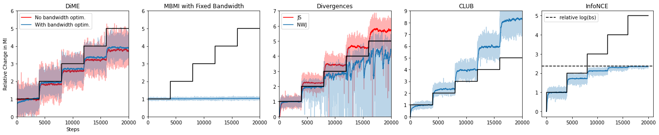
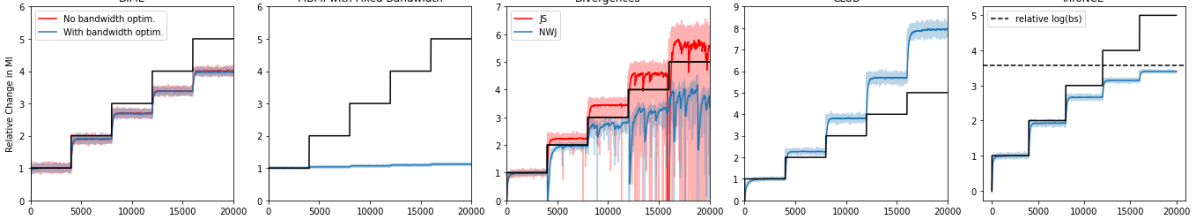
Figure 1: Performance of different estimators of MI for a toy correlated Gaussian dataset with increasing correlation over time. The black staircase line denotes the relative increase of true MI of the dataset. (top) Trained with batch size of 64 and using joint critics for variational estimators. (bottom) Trained with batch size of 1024 and using separable critics for variational estimators.

6 Experiments

We present several experiments showcasing potential applications for DiME. The main purpose of these experiments is to highlight the versatility of DiME when combined with other matrix-based information-theoretic quantities. As discussed previously, DiME is well suited for tasks involving the maximization of MI between random variables and assigns more value to simpler configurations that exhibit higher dependence. This can be used in contrastive learning and representation learning when trying to maximize dependence between two views of data, e.g. Wang et al. [2015], Oord et al. [2018], Hjelm et al. [2018], Zbontar et al. [2021].

Let $\mathbf{X}^{(1)}=\left\{x_{i}^{(1)}\right\}_{i=1}^{N}$ and $\mathbf{X}^{(2)}=\left\{x_{i}^{(2)}\right\}_{i=1}^{N}$ be paired sets of instances from two different views of some latent variable. The goal is to train encoders $f_{1}\in\mathcal{F}_{1}$ and $f_{2}\in\mathcal{F}_{2}$ (potentially with shared weights) in order to maximize the MI between the encoded representations by using DiME,

$$\underset{f_{1}\in\mathcal{F}_{1},f_{2}\in\mathcal{F}_{2}}{\operatorname{maximize}}\operatorname{DiME}_{\alpha}\left(f_{1}(\mathbf{X}^{(1)}),f_{2}(\mathbf{X}^{(2)}),\theta\right),$$ (10)

where $\theta$ is a shared kernel parameter. We apply our objective function in two multiview datasets and assess the results on the downstream tasks of classification and latent factor disentanglement.

6.1 Multiview MNIST

We follow the work of Wang et al. [2015] in constructing a multiview MNIST dataset with two views. The first view contains digits rotated randomly between $-45$ and $45$ degrees. The second view contains digits with added noise sampled uniformly from $[0,1]$, clamping to one all values in excess of one. The second view is then shuffled so that paired images are different instances from the same class. With this setup, the only information shared between views is the class label. We thus expect a maximization of dependence between the shared representation between views to carry only the class label information.

We encode each view using separate encoders with CNN architectures described in Appendix C.1. DiME is optimized between the views as described in Equation 10. We use a Gaussian kernel with fixed bandwidth $\theta=\sqrt{D/2}$ for each view. A batch size of 3000 is used.

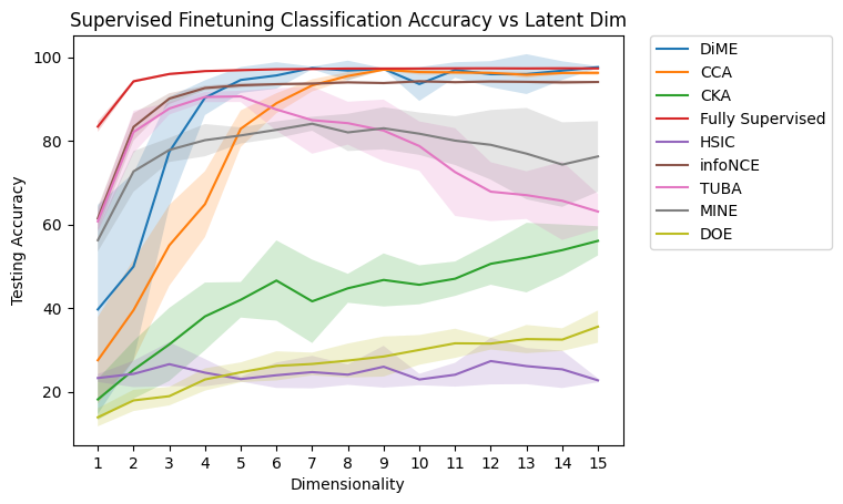
(a)

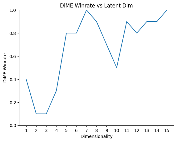
(b)

Figure 2: (left) Classification accuracy across dimensionality obtained via firstly training encoders with a dependence objective and then training a classifier consisting of one hidden layer after the frozen encoder. The accuracy of equivalently sized networks trained using direct supervision is included. (right) Win rate of DiME against other methods, excluding fully supervised.

We compare to the following baselines on the task of downstream classification accuracy: DCCA [Wang et al., 2015], CKA [Cortes et al., 2012, Kornblith et al., 2019], HSIC [Gretton et al., 2005], infoNCE [Oord et al., 2018], TUBA [Poole et al., 2019], MINE [Belghazi et al., 2018], and difference-of-entropies (DoE) [McAllester and Stratos, 2020]. We define downstream classification accuracy as training an encoder using a measure of dependence followed by the training of a supervised classifier with one hidden layer on the encoder’s output. Note that the encoder parameters are frozen after initial training. While the encoder never has access to labels during training, this approach is not unsupervised since label information is used in the pairings.

The downstream classification accuracies for varying latent dimensionalities, averaged over 10 random network initializations, are shown in Figure 2. We also provide DiME’s win rate, which we define as the proportion of the 10 trials that it is the best performing method (excluding fully supervised training). We observe that DiME wins a majority of the trials for higher latent dimensionalities. DiME also requires fewer latent dimensions to be competitive with the fully supervised training. However, DiME does have a higher variance than other top performing methods for specific dimensionalities.

6.2 Disentanglement of Latent Factors

So far we have extracted information that is common to two views. It is natural to ask if one can instead extract information that is exclusive to views. With the multiview MNIST dataset, exclusive information to View 1 would be rotations and for View 2 it would be noise. Because pairings are done by class label, exclusive information could also constitute latent factors such as stroke width, boldness, height, and width. In order to separate shared and exclusive information, we use the matrix-based conditional entropy defined in Equation 4. Let $\bm{S}^{(i)}$ and $\bm{E}^{(i)}$ define the shared and exclusive information in view $i\in\{1,2\}$ captured by the encoder $f_{i}$ for data $\bm{X}^{(i)}$. Then $f_{i}(\bm{X}^{(i)})=[\bm{S}^{(i)},\bm{E}^{(i)}]$, where the right side is a concatenation of dimensions over the batch. The matrix-based conditional entropy $S_{\alpha}(\mathbf{K}_{\bm{S}^{(i)}}|\mathbf{K}_{\bm{E}^{(i)}})$ quantifies the amount of uncertainty remaining for $\bm{S}^{(i)}$ (class label) after observing $\bm{E}^{(i)}$ (i.e. latent factors). Ideally, this quantity should be maximized so that observing exclusive information gleans nothing about shared information.

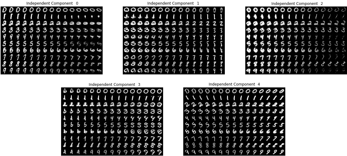
Figure 3: Walking on disentangled exclusive independent components. The walk is performed by encoding a digit prototype (center column) and modifying the exclusive dimensions. The leftmost and rightmost columns are moving -2 and +2 units, respectively, in the direction of the independent component, with evenly spaced steps in between.

Here, we use the same encoder setup as used in Section 6.1. To encourage the usage of exclusive dimensions by the encoder $f_{i}$, we also minimize reconstruction error by passing the full latent code through a decoder $g_{i}$. This is in contrast to Section 6.1 where only an encoder is needed. The reconstruction of $\bm{X}^{(i)}$ is denoted as $\hat{\bm{X}}^{(i)}=g_{i}(f_{i}(\bm{X}^{(i)}))$. A separate encoder/decoder pair is used for each view. The full optimization problem is

$$\begin{split}\underset{f_{1},g_{1},f_{2},g_{2}}{\operatorname{maximize}}\quad&\textrm{DiME}_{\alpha}(\bm{S}^{(1)},\bm{S}^{(2)},\theta)+S_{\alpha}(\mathbf{K}_{\bm{S}^{(1)}}|\mathbf{K}_{\bm{E}^{(1)}})+S_{\alpha}(\mathbf{K}_{\bm{S}^{(2)}}|\mathbf{K}_{\bm{E}^{(2)}})\\ &-\textrm{MSE}(\bm{X}^{(1)},\hat{\bm{X}}^{(1)})-\textrm{MSE}(\bm{X}^{(2)},\hat{\bm{X}}^{(2)}).\end{split}$$ (11)

We use this to learn 10 shared dimensions and 5 exclusive dimensions. Unlike variational autoencoders, which also learn latent factors in an information-theoretic fashion, we are not enforcing that each exclusive dimension is independent of the others [Kingma and Welling, 2019], but instead letting them have dependence [Cardoso, 1998, Hyvärinen and Hoyer, 2000, Casey and Westner, 2000, Von Kügelgen et al., 2021]. In order to visualize what exclusive factors are being learned, we calculate the independent components of the exclusive dimensions with parallel FastICA [Hyvärinen and Oja, 2000]. Using these independent components, we can start with a prototype and perform walks in the latent space in independent directions. By walking in a single independent direction, we intend to change only a single latent factor. In Figure 3, we walk on the five exclusive independent components of View 1. Qualitatively, it seems that they encode height, width, stroke width, roundness, and rotation.

6.3 Colored MNIST

Next we conduct experiments for learning disentangled representations by using DiME on the colored MNIST dataset, as in Sanchez et al. [2020]. Given a pair of images from the same class but from different views (colored background and colored foreground digits, see Figure 4(a)), we seek to learn a set of shared features that represent the commonalities between the images and disentangle the exclusive features of each view. These representations are useful for certain downstream tasks, such as image retrieval by finding similar images to a query based on its shared or exclusive features.

We maximize the MI between the shared representations captured by a single encoder $f_{\textrm{sh}}$ and minimize the MI of the shared and exclusive features captured by a separate encoder $f_{\textrm{ex}}$ to encourage the disentanglement of the two components. In particular, $f_{\textrm{sh}}(\mathbf{X})=\mathbf{S}$ encodes the shared features of the two views (class-dependent features), and $f_{\textrm{ex}}(\mathbf{X})=\mathbf{E}=[\mathbf{V},\mathbf{Z}]$ extracts the class-independent attributes so that $\mathbf{V}$ contains the exclusive features of each view (view-dependent features). $\mathbf{Z}$ is used to encode residual latent factors needed for reconstruction.

Our training procedure consists of two steps to follow the work of Sanchez et al. [2020]. First, because we want $f_{\textrm{sh}}$ to learn a shared space that is invariant to the view, we first maximize the MI between the shared representations of both views $\mathbf{S}^{(1)}$ and $\mathbf{S}^{(2)}$ via DiME as in Equation 10. The same encoder $f_{\textrm{sh}}$ is used for both views. Second, once the shared representation is learned, we freeze the shared encoder and train the exclusive encoder $f_{\textrm{ex}}$. To disentangle the three latent subspaces, we minimize the matrix-based MI between $\mathbf{S}$ and $\mathbf{E}$ and minimize the matrix-based MI between $\mathbf{V}$ and $\mathbf{Z}$. This procedure encourages the exclusive encoder not to learn features that were already learned by the shared encoder. Additionally, we place a conditional prior on $\mathbf{V}=[\mathbf{V}_{1},\mathbf{V}_{2}]$ such that $\mathbf{V}^{(1)}=[\mathbf{V}_{1},\mathbf{0}]$ and $\mathbf{V}^{(2)}=[\mathbf{0},\mathbf{V}_{2}]$ intending different subspaces to independently encode the view-exclusive generative factors (see Figure 4(d)). We achieve this by minimizing the Jensen-Rényi divergence (JRD) [Osorio et al., 2022] of the view-exclusive features to samples from two mutually exclusive uniform random variables from 0 to 1, which we denote as $\mathbf{P}$. To ensure that features have high MI with the images, we also train a decoder $g$ that will reconstruct the original images using all three latent subspaces. We train the exclusive encoder by optimizing $f_{\textrm{ex}},g$ to minimize the loss function $\mathcal{L}_{\textrm{ex}}=I_{\alpha}(\mathbf{S},\mathbf{E})+I_{\alpha}(\mathbf{V},\mathbf{Z})+D_{\alpha}(\mathbf{V}||\mathbf{P})+\textrm{MSE}(\mathbf{X},\hat{\mathbf{X}})$. Exact model details are provided in Appendix D.

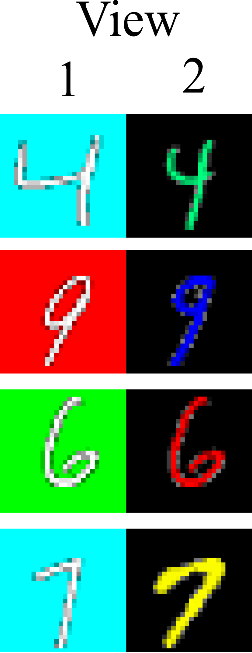
(a)

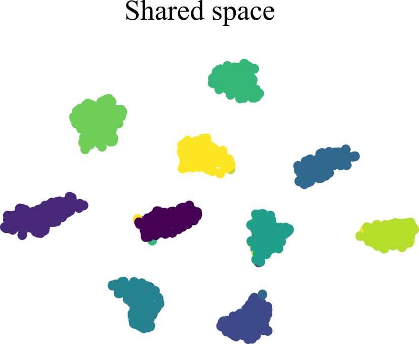
(b)

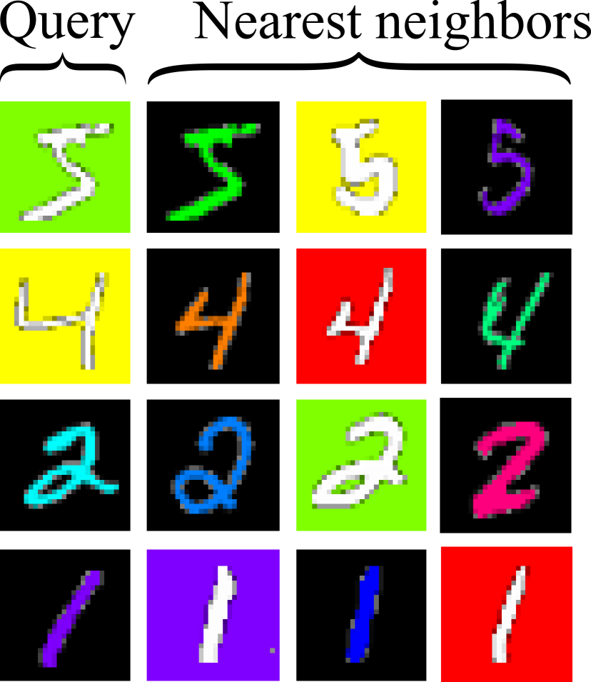
(c)

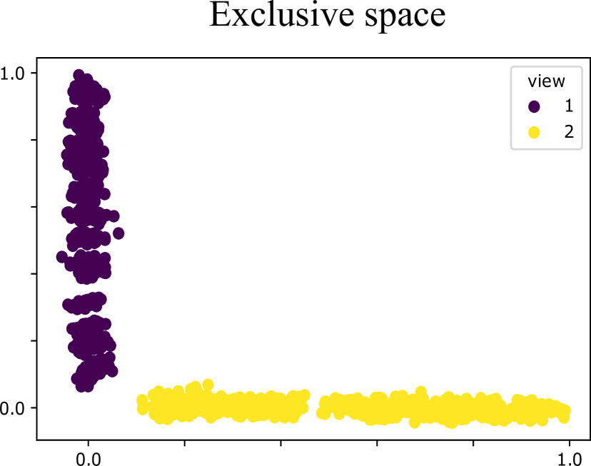
(d)

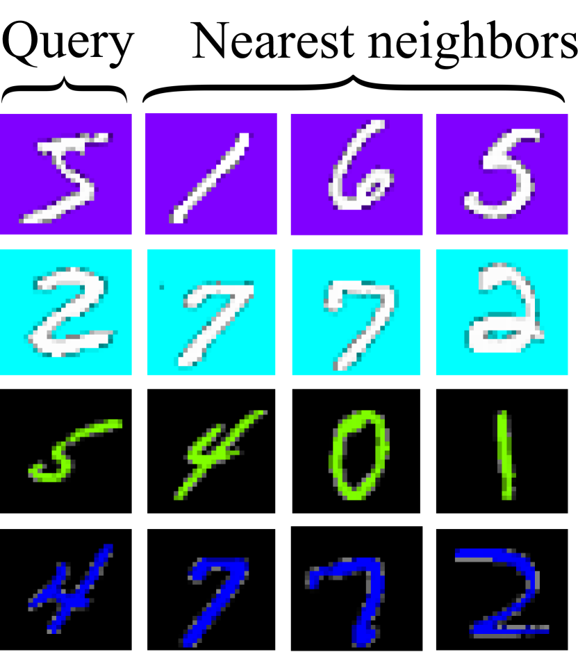
(e)

Figure 4: (a) Example of a pair of images from the multiview colored MNIST: view 1 corresponds to background colored digits and view 2 to foreground colored digits. (b) t-SNE of the shared features learned via DiME. Colors represent different digit labels. (c) Image retrieval by finding nearest neighbors on the shared features. (d) view-exclusive features learned by minimizing JRD to a desired prior. (e) Image retrieval by finding nearest neighbors on the view-exclusive features

A t-SNE visualization of the learned shared features (Figure 4(b)) shows how digits from the same class are grouped into the same clusters regardless of the view. This is corroborated by image retrieval by finding the nearest neighbors to the shared representation of a query image (Figure 4(c)). DiME captures the common attributes between the two views, which in this case is class information. On the other hand, the learned view-exclusive features (Figure 4(d)) are class-agnostic and for a given query, the exclusive space nearest neighbors correspond to the same background/foreground color. This is independent of the digit class (Figure 4(e)). To further support the quality of disentanglement, we give a visualization in Appendix D.3 where we perform style transfer.

Method	DN	B	F
Ideal	100%	8.33%	8.33%
S. 2020	94.48%	8.22%	8.83%
GG. 2018	95.42%	99.56%	29.81%
MINE	98.92%	11.24 %	12.11%
DiME	98.93%	8.79%	8.41%

Method	DN	B	F
Ideal	10.00%	100%	100%
S. 2020	13.20%	99.99%	99.92%
GG. 2018	99.99%	71.63%	29.81%
MINE	10.85%	69.38%	70.24%
DiME	10.30%	98.84%	84.3%

Table 1: Digit number (DN), Background (B) and Foreground (F) color accuracy using the (left) shared representations and (right) exclusive representations. Note that S. 2020 refers to Sanchez et al. [2020] and GG. 2018 refers to Gonzalez-Garcia et al. [2018].

As in Sanchez et al. [2020], we evaluate the disentanglement of the shared and exclusive features by performing some classification experiments. Ideally, a digit classifier trained on the shared features should accurately classify the digit label with poor color classification. Conversely, the classification of exclusive features should perform well in identifying color and randomly for digit labels. We train a classifier and compare our results to Sanchez et al. [2020], Gonzalez-Garcia et al. [2018], and MINE in Table 1. DiME achieves the highest digit number classification accuracy on shared features. Additionally, the foreground and background color accuracy is close to a random guess, verifying the disentanglement between shared and exclusive features. For the MINE baseline, we replaced DiME with MINE while keeping the rest of the losses. When using MINE (or other MI estimators), it is necessary to tune the kernel bandwidth for matrix-based quantities. On the contrary, DiME naturally adjusts the data with a fixed bandwidth ($\sqrt{D/2}$ was used) to make the representations suitable for matrix-based quantities. For MINE, we tested 5 different values of kernel bandwidth selected in a $\log$ space around $\sqrt{D/2}$ and show the best results.

7 Conclusions

We proposed DiME, a quantity that behaves like MI and can be estimated directly from data. DiME is built using matrix-based entropy, which uses kernels to measure uncertainty in the dataset. We compared the behavior of DiME as an MI estimator to variational estimators and showed it was well-behaved for sufficiently large batch sizes. Unlike variational estimators, DiME does not require a critic network and is calculated in the same space as data representations. We applied DiME to the problems of multiview representation learning and factor disentanglement. To handle the variance of DiME, which can be very large, we are exploring alternatives to the Gram matrix formulation. For instance, by working directly in the feature space, we can aggregate results from small batches and reduce the variance of the estimators. There are several methods to provide an explicit feature space, such as using Random Fourier Feature approximations [Rahimi and Recht, 2007] to kernels.

8 Limitations

Below are some limitations of this work:

• Sensitivity to Batch Size As pointed out in Section 5, one method of reducing the variance of DiME is by increasing the batch size. However, we acknowledge that not all datasets are amenable to large batch sizes. In such cases, other methods can be used to reduce the variance of DiME such as increasing the number of permutations used to approximate the expectation.

• Minimization of Mutual Information Since the self-regulation of DiME comes from maximizing the difference of entropies, applications that seek to minimize mutual information would require solving a $\operatorname{minmax}$ optimization. In such cases, alternatives to DiME seem preferable.

• Estimation of Shannon’s Mutual Information As mentioned previously, DiME is not an estimator of Shannon’s MI. It shares several properties with Shannon’s MI that allow it to be used, for instance, in tasks of maximizing MI. However, DiME is not able to be used for tasks that require actual estimation of Shannon’s MI where measurement units (bits or nats) are important.

9 Acknowledgements

This material is based upon work supported by the Office of the Under Secretary of Defense for Research and Engineering under award number FA9550-21-1-0227.

Appendix A Behavior of DiME with respect to Kernel Bandwidth

In Section 3, we argue that DiME ”moves from small to large and back to small as we decrease the kernel bandwidth $\sigma$ from $\sigma=\infty\rightarrow\sigma=0$”. In other words, there exists a maximal value of DiME for some finite $\sigma\neq 0$. This is in contrast to matrix-based mutual information which achieves a maximum value of $\ln(n)$ when $\sigma=0$ due to saturation. These behaviors are shown in Figure 5.

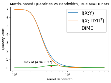
(a)

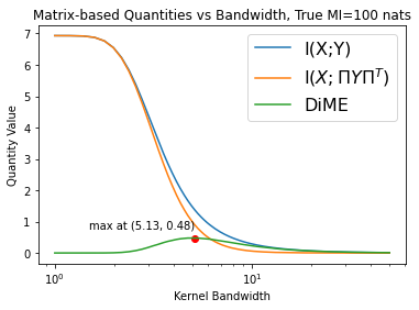
(b)

Figure 5: Comparison of DiME and matrix-based MBMI as kernel bandwidth $\sigma$ is changed. $X$ and $Y$ are drawn from the correlated Gaussian dataset mentioned in Section 5. $X$ and $Y$ have $n=1024$ samples each. The Shannon MI between $X$ and $Y$ is (top) 10 nats and (bottom) 100 nats.

Appendix B Further Details of Variational Bounds Comparisons

B.1 Alternative Plot for Figure 1

We showed in Figure 1 a relative comparison of DiME to variational MI estimators. This relative comparison shows how changes in the underlying true MI proportionally affect the estimators. We chose to show relative quantities, rather than the actual quantity values, because matrix-based information-theoretic quantities are on a different scale than the true MI and the other estimators. Here in Figure 6, we show an alternative version of the plot which depicts the actual quantity values. Note that there are two different y-axes in some graphs: the left y-axis shows the quantity values and the right y-axis shows the true MI.

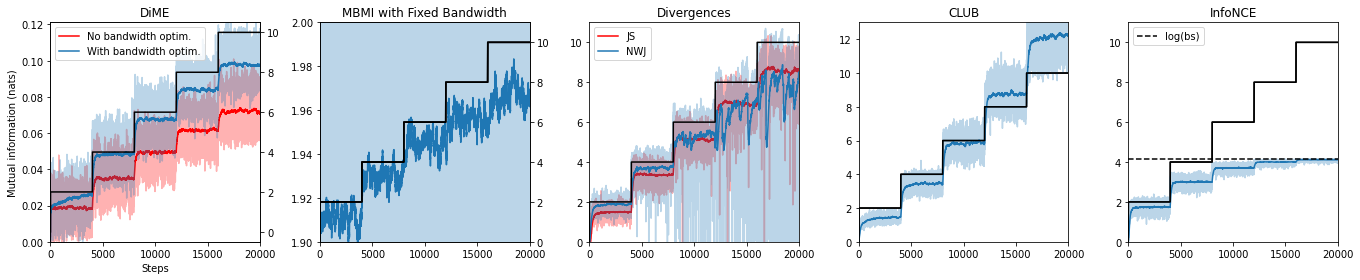
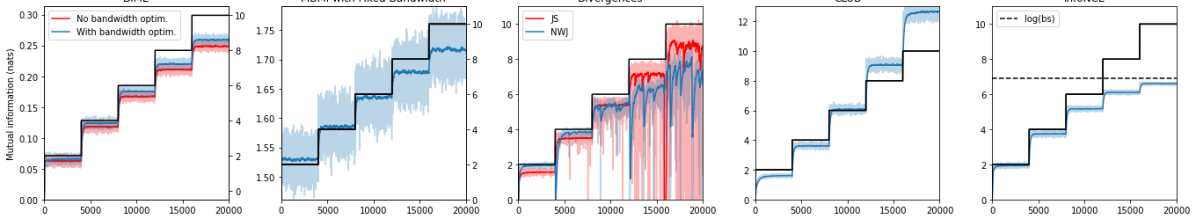
Figure 6: Performance of different estimators of MI for a toy correlated Gaussian dataset with increasing correlation over time. The black staircase line denotes the true MI of the dataset. (top) Trained with batch size of 64 and using joint critics for variational estimators. (bottom) Trained with batch size of 1024 and using separable critics for variational estimators.

B.2 Behavior of DiME with respect to Batch Size and Dimensionality

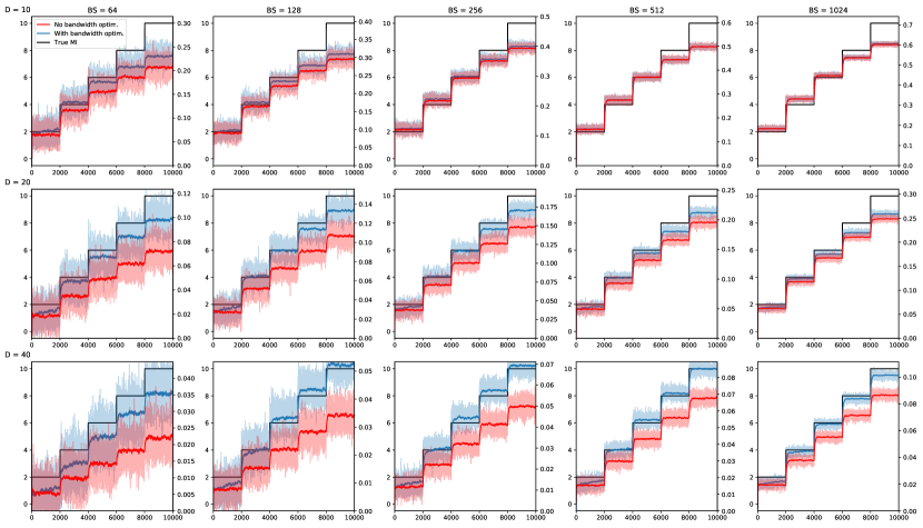
(a) For varying batch sizes (columns) and dimensionalities (rows), we use DiME to approximate the MI of a toy dataset. We use a Gaussian kernel as DiME’s kernel function. Learned kernel bandwidths are plotted below. For the fixed kernel bandwidths, we use $\sigma=\sqrt{D/2}$

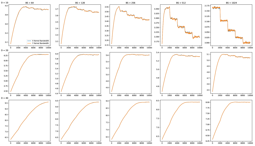
(b) Values of learned kernel bandwidths. Each plot corresponds to the plot in the same position in the above figure.

Figure 7: Behavior of DiME as data dimensionality and batch size are varied.

We display how DiME behaves by changing the batch size and dimensionality in Figures 7(a) and 7(b). We use the same toy dataset (from Poole et al. [2019]) as described in Section 5. Note that the true MI is on a different scale from DiME, and the DiME y-axis is on the right-hand side of each graph. Here we use only one random permutation to approximate the expectation in DiME. The darker lines are weighed running averages with a window size of 100. A few critical behaviors can be observed in 7(a):

1. Increasing batch size decreases variance and increases the bias

2. Increasing dimensionality increases variance and decreases the bias

3. Kernel bandwidth optimization has a larger effect in high dimensionalities

These behaviors are important to keep in mind when using DiME. It may be possible to normalize DiME in such a way that helps stabilize its bias with regard to changes in batch size or dimensionality, but we leave that to future work.

Appendix C Further Details of Multiview MNIST Experiments

C.1 Multiview MNIST Model Details

Here we describe the model architecture used in Sections 6.1 and 6.2.

In Section 6.1, we trained the encoder architecture described in Table 2. To test downstream accuracy on the rotated view, we used a linear classifier with one hidden layer mapping (D → 1024 → 10). Separate encoders and classifiers were used for each view. These architectures were used for DiME and all baselines. We used Adam to train with a learning rate of 0.0005, batch size of 3000, for 100 epochs. The latent dimensionality D was ranged between 1 and 15. For the DiME and CKA objective functions, we used the Gaussian kernel with a fixed kernel parameter of $\sqrt{D/2}$.

In Section 6.2 , we used both the encoder and decoder described in Table 2. We used Adam to train with a learning rate of 0.0005, batch size of 3000, for 100 epochs. We used DiME as described in the preceding paragraph. We use a shared latent dimensionality of 10 and an exclusive dimensionality of 5. Thus the total latent dimensionality (D in Table 2) is 15. Note that DiME only operates on the 10 shared latent dimensions from each view, while conditional entropy operates on both shared latent dimensions and exclusive dimensions. Additionally, the decoder uses the entire 15 latent dimensions.

Table 2: Description of the architectures employed in multiview MNIST experiments

Encoder	Decoder
Input: $28\times 28\times 1$	Input: $1\times 1\times D$
$3\times 3$ conv, $8$ out channel, stride $2$, padding $1$	Linear $D$ in dimensions, $1024$ out dimensions
ReLU	ReLU
$3\times 3$ conv, $16$ out channel, stride $2$, padding $1$	Linear $1024$ in dimensions, $3*3*32$ out dimensions
Batch Normalization	reshape to $32\times 3\times 3$
ReLU	$3\times 3$ convTrans, $16$ out channel, stride $2$
$3\times 3$ conv, $32$ out channel, stride $2$	Batch Normalization
ReLU	ReLU
LazyLinear, $1024$ out dimensions	$3\times 3$ convTrans, $8$ out channel, stride $2$, padding=$1$, output padding=$1$
Linear, $1024$ in dimensions, $D$ out dimensions	Batch Normalization
	ReLU
	$3\times 3$ convTrans, $1$ out channel, stride $2$, padding=$1$, output padding=$1$

Appendix D Further Details of Colored MNIST Experiments

D.1 Colored MNIST Model Details

For the shared encoder $f_{sh}$ we train the architecture shown in Table 3. Here, we used Adam with a learning rate of 0.0001 and a batch size of 1500 for 50 epochs to learn 10 features. Once this model is trained, we freeze it and learn the exclusive encoder $f_{ex}$ and the decoder $g$ with Adam with a learning rate of 0.0001, batch size of 64 for 100 epochs. The architecture of $f_{ex}$ is the same used for $f_{sh}$ and the decoder architecture is also shown in 3. The dimensionality of $\mathbf{S},\mathbf{V}$ and $\mathbf{Z}$ are 10, 2 and 6 respectively.

Table 3: Description of the architectures employed in the colored multiview MNIST experiments

Encoder	Decoder
Input: $28\times 28\times 3$	Input: $1\times 1\times D$
$3\times 3$ conv, $32$ out channel, stride $1$, padding $1$	Linear $D$ in dimensions, $1024$ out dimensions
ReLU	ReLU
$3\times 3$ conv, $64$ out channel, stride $1$, padding $1$	Linear $1024$ in dimensions, $4\times 4\times 256$ out dimensions
ReLU	ReLU
2D Maxpooling $2\times 2$	$3\times 3$ convTrans, $256$ out channel, stride $2$, padding=$1$
$3\times 3$ conv, $128$ out channel, stride $1$, padding $1$	ReLU
ReLU	$3\times 3$ conv, $128$ out channel, stride $1$, padding $1$
$3\times 3$ conv, $128$ out channel, stride $1$, padding $1$	ReLU
ReLU	$3\times 3$ conv, $128$ out channel, stride $1$, padding $1$
2D Maxpooling $2\times 2$	ReLU
$3\times 3$ conv, $256$ out channel, stride $1$, padding $1$	$4\times 4$ conv, $64$ out channel, stride $2$, padding $1$
ReLU	ReLU
2D Maxpooling $2\times 2$	$3\times 3$ conv, $32$ out channel, stride $1$, padding $1$
Linear, $144\times 4\times 4$ in dimensions, 1024 out dimensions	ReLU
Linear, 1024 in dimensions, D out dimensions	$4\times 4$ conv, $3$ out channel, stride $2$, padding $1$

D.2 Disentanglement of the residual latent factors

To evaluate what the residual factors $\mathbf{Z}$ are capturing, we extracted their independent components to see if they capture different aspects of the digits. In Figure 8 we walk on the six independent components which seem to encode different prototypes of the digits, except for the independent component 1 which clearly encodes the rotation of the digit.

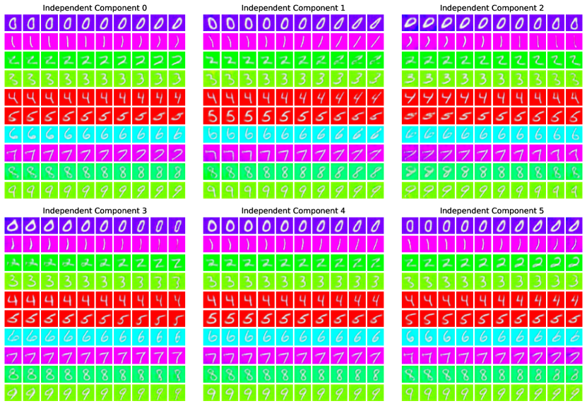
(a) ICA walks on View 1

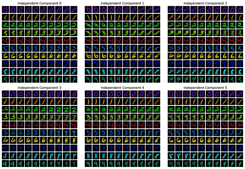
(b) ICA walks on View 2

Figure 8: Walking on the independent components of the residual latent factors of the colored MNIST dataset.

D.3 Style Transfer

To further support the quality of the shared features learned by DiME, we generate samples by keeping the shared representation fixed and moving along the view-exclusive dimensions. In Figures 9(a) and 9(b) we can see how the digit content is well preserved as the view generative factor is changing. Specifically, each row corresponds to a random digit image selected from the dataset. We encode this image, modify the view-exclusive dimension, and visualize the decoded image.

This approach is also well suited for style transfer, by exchanging the style (exclusive $E$) between a query and a reference image while keeping the content (shared $S$) intact. Without any additional training required, we display style transfer in Figure 9(c).

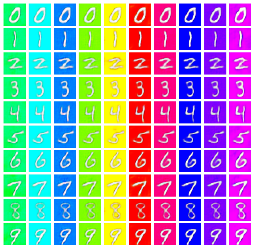
(a)

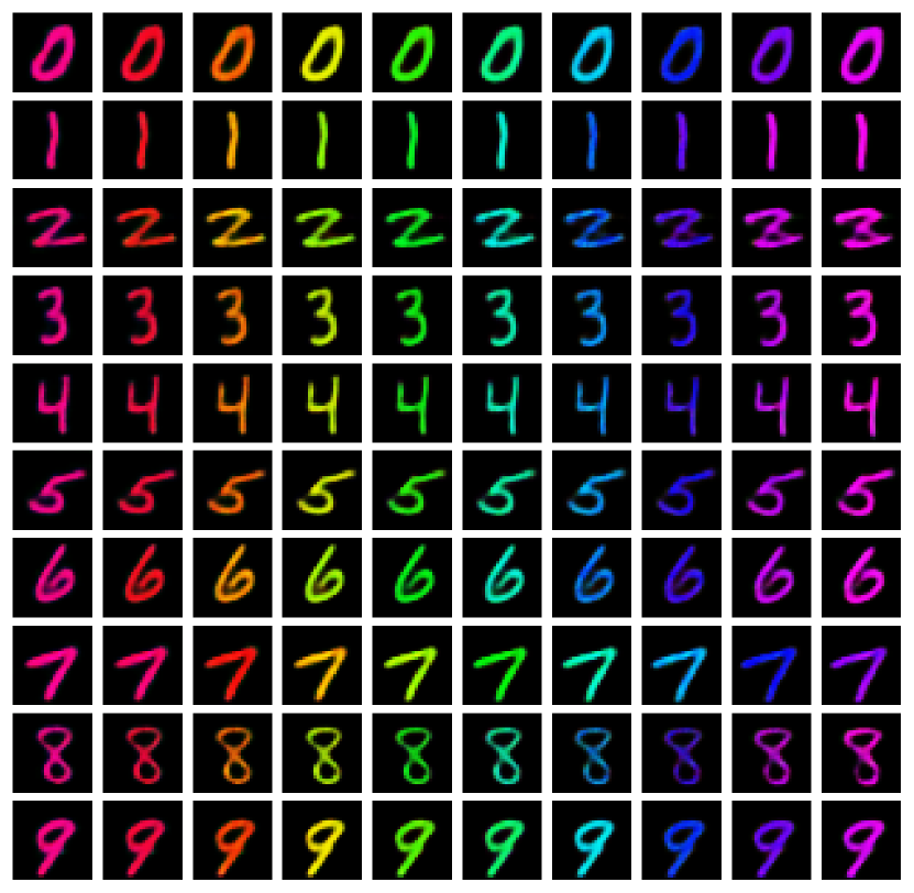
(b)

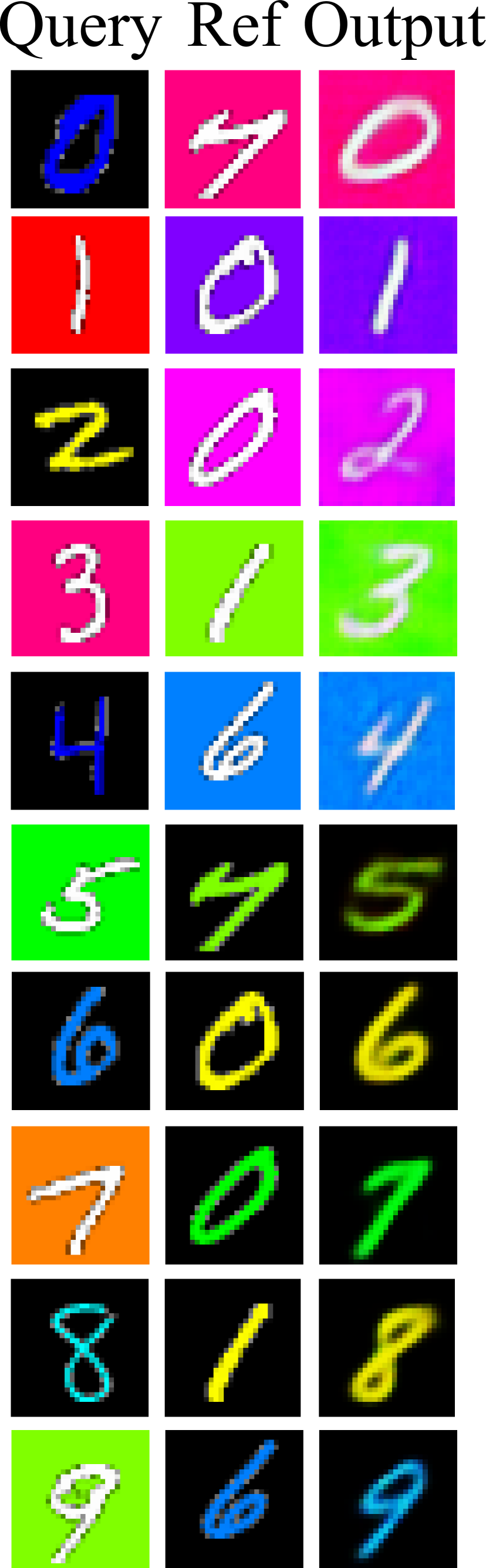
(c)

Figure 9: Disentangling of generative factors in the multiview colored MNIST dataset. (a) Walking on the exclusive dimension of view 1. (b) Walking on the exclusive dimension of view 2. (c) Style transfer results by swapping exclusive dimensions.

Appendix E DiME-GANs

Motivated by the relation between MI and Jensen-Shannon divergence, we propose training of GANs as an alternating optimization between two competing objectives based on DiME. The purpose of this is not to break new ground in GANs, but to instead highlight the versatility of DiME. Similar to MMD-GAN Li et al. [2017], our discriminator network $f_{\theta}$ maps samples from data space $\mathcal{X}$ to a representation space $\mathcal{Y}$, and the generator network $g_{\psi}$ maps samples from the noise space $\mathcal{Z}$ to data space $\mathcal{X}$.

To train the discriminator, we use DiME to maximize the MI between samples of a mixture distribution and an indicator variable. The mixture distribution has two components: the distribution of real samples and the distribution of samples from a generator. The indicator variable is paired with each sample drawn from the mixture and indicates the component (real or fake) from which the sample came from. To train the generator, we maximize the matrix-based conditional entropy of the indicator variable given a sample from the mixture. This is equivalent to minimizing the matrix-based MI between the mixture and the indicator variable. Since the matrix-based MI is an upper bound of DiME, each generator update tries to reduce DiME by pushing down this upper bound. Conversely, each discriminator step tunes the representation space such that the upper bound given by the matrix-based MI is tight.

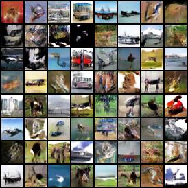
Figure 10: Samples generated using DiME-GAN

Figure 10 shows samples from DiME-GAN trained on CIFAR10 dataset. For the kernel we use the Laplacian kernel defined as $\kappa_{\sigma}(x,y)=e^{-\frac{\sum_{i=1}^{D}|(x)_{i}-(y)_{i}|}{\sigma}}$ with sigma fixed $\sigma=\sqrt{D/2}$. The discriminator objective tunes the parameters of $f_{\theta}$. For each iteration, we use 64 images from the true distribution and 64 images sampled from the generator network. Both optimizers use Adam with $lr=0.00005$. The architecture is similar to DCGAN, but without batch-normalization and gradient clipping during training. Details of the employed architecture and hyperparameters are provided in table 5.

E.1 Details of the GAN and Objective Function

We have two mappings: a discriminator $f_{\theta}$ network that maps points from data space $\mathcal{X}$ to representation space $\mathcal{Y}$, and a generator network $g_{\psi}$that maps noise samples from $\mathcal{Z}$ to data space $\mathcal{X}$. Namely, for CIFAR10, $\mathcal{X}\subset\mathbb{R}^{32\cdot 32\cdot 3}$, $\mathcal{Z}\subseteq\mathbb{R}^{D_{Z}}$, and $\mathcal{Y}\subseteq\mathbb{R}^{D_{Y}}$. Details of the architecture of the discriminator and generator networks are provided in Table 5

Each full iteration of the algorithm is comprised of two updates: an update for the discriminator, and an update for the generator. Let $\mathbf{X}_{r}$ be the size $N_{\textrm{batch}}$ batch of real samples, $\mathbf{X}_{f}=g_{\psi}\left(\mathbf{Z}\right)$ a batch of generated samples, and $\mathbf{X}=\operatorname{cat}\{\mathbf{X}_{r},\mathbf{X}_{f}\}$ a concatenated samples. Associated to $\mathbf{X}$ we have the label vector $\mathbf{l}$ that indicates which samples in $\mathbf{X}$ come from $\mathbf{X}_{r}$ and $\mathbf{X}_{f}$, respectively. The discriminator update is based on DiME, which measures the dependence between $\mathbf{X}$ and $\mathbf{l}$. At each iteration, we update $\theta$ to increase the difference of entropies.

$$\mathbb{E}_{\bm{\Pi}}\left[S_{\alpha}(\mathbf{K}_{\mathbf{X}}(\theta)\circ\bm{\Pi}\mathbf{K}_{\mathbf{l}}\bm{\Pi}^{T})\right]\\ -S_{\alpha}(\mathbf{K}_{\mathbf{X}}(\theta)\circ\mathbf{K}_{\mathbf{l}}),$$ (12)

where $\left(\mathbf{K}_{\mathbf{l}}\right)_{ij}=1$ if $i$ and $j$ are both real or fake images, and $0$ otherwise. The kernel between two images corresponds to the composition of the discriminator mapping $f_{\theta}$ followed by a positive definite kernel $\kappa:\mathcal{Z}\times\mathcal{Z}\mapsto\mathbb{R}$, namely, $\left(\mathbf{K}_{\mathbf{X}}(\theta)\right)_{ij}=\kappa(f_{\theta}(x_{i}),f_{\theta}(x_{j}))$. The generator update is based on matrix-based conditional entropy of $\mathbf{l}$ given $\mathbf{Y}=f_{\theta}(\mathbf{X})$. In this step, the parameters of the discriminator remain fixed and the parameters $\psi$ of the generator are updated so that the conditional entropy,

$$S_{\alpha}(\mathbf{K}_{\mathbf{Y}}(\psi)\circ\mathbf{K}_{\mathbf{l}})-S_{\alpha}(\mathbf{K}_{\mathbf{Y}}(\psi)),$$ (13)

increases. In this case, the gradients of the objective backpropagate to the generator network, since $\mathbf{Y}_{f}=f_{\theta}(g_{\psi}(\mathbf{Z}))$. To compute the Gram matrix, we use the same kernel $\kappa$ as in Equation 12. To optimize parameters, we use Adam with learning rate $lr=0.00005$ and $\beta_{1}=0.5$. Note that there is one optimizer for the discriminator and another for the generator. For the kernel $\kappa$ we tried several options, listed in Table 4. In all experiments, we set the kernel parameter to $\sigma=\sqrt{D/2}$, for $x\in\mathbb{R}^{D}$. Figure 11 shows examples of generated images after training the GAN with the DiME objective for the kernels described in Table 4.

Table 4: Kernel functions that we tried in DiME-GAN experiments

Kernel	$\kappa(x_{i},x_{j})$
Gaussian	$\exp{(\frac{1}{2\sigma^{2}}\|x_{i}-x_{j}\|_{2}^{2})}$
Factorized Laplacian	$\exp{(\frac{1}{\sqrt{2}\sigma}\|x_{i}-x_{j}\|_{1})}$
Elliptical Laplacian	$\exp{(\frac{1}{\sqrt{2}\sigma}\|x_{i}-x_{j}\|_{2})}$

Table 5: Description of the architectures employed in DiME-GAN experiments

Discriminator	Generator
Input: $32\times 32\times 3$	Input: $1\times 1\times 100$
$4\times 4$ conv, $64$ out Channel, stride $2$, padding $1$	$4\times 4$ convTrans, $512$ out Channel, stride $1$, padding $0$
leakyReLU($0.2$)	leakyReLU $0.2$
$4\times 4$ conv, $128$ out Channel, stride $2$, padding $1$	$4\times 4$ convTrans, $256$ out Channel, stride $2$, padding $1$
leakyReLU $0.2$	leakyReLU $0.2$
$4\times 4$ conv, $256$ out Channel, stride $2$, padding $1$	$4\times 4$ convTrans, $128$ out Channel, stride $2$, padding $1$
$4096$ fullyConnected, $64$ out Dims	leakyReLU $0.2$
	$4\times 4$ convTrans, $3$ out Channel, stride $2$, padding $1$
	$\tanh$

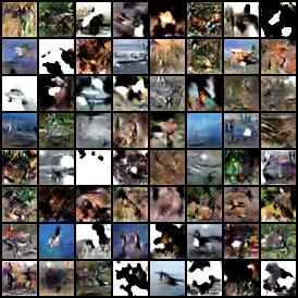
(a) Gaussian kernel

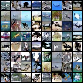
(b) Elliptical Laplacian kernel

(c) Factorized Laplacian kernel

Figure 11: Generated Images for DiME-GAN trained with different kernels

References

- Bachman et al. [2019] Philip Bachman, R Devon Hjelm, and William Buchwalter. Learning representations by maximizing mutual information across views. Advances in Neural Information Processing Systems, 32, 2019.
- Belghazi et al. [2018] Mohamed Ishmael Belghazi, Aristide Baratin, Sai Rajeswar, Sherjil Ozair, Yoshua Bengio, Aaron Courville, and R Devon Hjelm. Mine: mutual information neural estimation. arXiv preprint arXiv:1801.04062, 2018.
- Bhatia [1997] Rajendra Bhatia. Matrix Analysis, volume 169. Springer, 1997. ISBN 0387948465.
- Camilo et al. [2019] Giancarlo Camilo, Gabriel T. Landi, and Sebas Eliëns. Strong subadditivity of the Rényi entropies for bosonic and fermionic gaussian states. Physical Review B, 99(4), jan 2019. doi: 10.1103/physrevb.99.045155. URL https://doi.org/10.1103%2Fphysrevb.99.045155.
- Cardoso [1998] J-F Cardoso. Multidimensional independent component analysis. In Proceedings of the 1998 IEEE International Conference on Acoustics, Speech and Signal Processing, ICASSP’98 (Cat. No. 98CH36181), volume 4, pages 1941–1944. IEEE, 1998.
- Casey and Westner [2000] Michael A Casey and Alex Westner. Separation of mixed audio sources by independent subspace analysis. In ICMC, pages 154–161, 2000.
- Cheng et al. [2020] Pengyu Cheng, Weituo Hao, Shuyang Dai, Jiachang Liu, Zhe Gan, and Lawrence Carin. Club: A contrastive log-ratio upper bound of mutual information. In International Conference on Machine Learning, pages 1779–1788. PMLR, 2020.
- Cortes et al. [2012] Corinna Cortes, Mehryar Mohri, and Afshin Rostamizadeh. Algorithms for learning kernels based on centered alignment. The Journal of Machine Learning Research, 13:795–828, 2012.
- Gonzalez-Garcia et al. [2018] Abel Gonzalez-Garcia, Joost Van De Weijer, and Yoshua Bengio. Image-to-image translation for cross-domain disentanglement. Advances in Neural Information Processing Systems, 31, 2018.
- Gretton et al. [2005] Arthur Gretton, Olivier Bousquet, Alex Smola, and Bernhard Schölkopf. Measuring statistical dependence with Hilbert-Schmidt norms. In International Conference on Algorithmic Learning Theory, pages 63–77. Springer, 2005.
- Hjelm et al. [2018] R Devon Hjelm, Alex Fedorov, Samuel Lavoie-Marchildon, Karan Grewal, Phil Bachman, Adam Trischler, and Yoshua Bengio. Learning deep representations by mutual information estimation and maximization. arXiv preprint arXiv:1808.06670, 2018.
- Huntington et al. [2021] Kelsey E Huntington, Anna D Louie, Chun Geun Lee, Jack A Elias, Eric A Ross, and Wafik S El-Deiry. Cytokine ranking via mutual information algorithm correlates cytokine profiles with presenting disease severity in patients infected with SARS-CoV-2. Elife, 10, 2021.
- Hyvärinen and Hoyer [2000] Aapo Hyvärinen and Patrik Hoyer. Emergence of phase-and shift-invariant features by decomposition of natural images into independent feature subspaces. Neural Computation, 12(7):1705–1720, 2000.
- Hyvärinen and Oja [2000] Aapo Hyvärinen and Erkki Oja. Independent component analysis: algorithms and applications. Neural Networks, 13(4-5):411–430, 2000.
- Kim and Mnih [2018] Hyunjik Kim and Andriy Mnih. Disentangling by factorising. In International Conference on Machine Learning, pages 2649–2658. PMLR, 2018.
- Kingma and Ba [2014] Diederik P Kingma and Jimmy Ba. Adam: A method for stochastic optimization. arXiv preprint arXiv:1412.6980, 2014.
- Kingma and Welling [2019] Diederik P Kingma and Max Welling. An introduction to variational autoencoders. Foundations and Trends in Machine Learning, 12(4):307–392, 2019.
- Kornblith et al. [2019] Simon Kornblith, Mohammad Norouzi, Honglak Lee, and Geoffrey Hinton. Similarity of neural network representations revisited. In International Conference on Machine Learning, pages 3519–3529. PMLR, 2019.
- Kraskov et al. [2004] Alexander Kraskov, Harald Stögbauer, and Peter Grassberger. Estimating mutual information. Physical Review E, 69(6):066138, 2004.
- Li et al. [2017] Chun-Liang Li, Wei-Cheng Chang, Yu Cheng, Yiming Yang, and Barnabás Póczos. Mmd gan: Towards deeper understanding of moment matching network. In Proceedings of the 31st International Conference on Neural Information Processing Systems, NIPS’17, page 2200–2210, Red Hook, NY, USA, 2017. Curran Associates Inc. ISBN 9781510860964.
- Linsker [1988] Ralph Linsker. Self-organization in a perceptual network. Computer, 21(3):105–117, 1988.
- Majdara and Nooshabadi [2022] Aref Majdara and Saeid Nooshabadi. Efficient density estimation for high-dimensional data. IEEE Access, 10:16592–16608, 2022.
- McAllester and Stratos [2020] David McAllester and Karl Stratos. Formal limitations on the measurement of mutual information. In International Conference on Artificial Intelligence and Statistics, pages 875–884. PMLR, 2020.
- Nguyen et al. [2010] XuanLong Nguyen, Martin J Wainwright, and Michael I Jordan. Estimating divergence functionals and the likelihood ratio by convex risk minimization. IEEE Transactions on Information Theory, 56(11):5847–5861, 2010.
- Oord et al. [2018] Aaron van den Oord, Yazhe Li, and Oriol Vinyals. Representation learning with contrastive predictive coding. arXiv preprint arXiv:1807.03748, 2018.
- Orlitsky and Suresh [2015] Alon Orlitsky and Ananda Theertha Suresh. Competitive distribution estimation: Why is good-turing good. Advances in Neural Information Processing Systems, 28, 2015.
- Orlitsky et al. [2003] Alon Orlitsky, Narayana P Santhanam, and Junan Zhang. Always good turing: Asymptotically optimal probability estimation. Science, 302(5644):427–431, 2003.
- Osorio et al. [2022] Jhoan Keider Hoyos Osorio, Oscar Skean, Austin J Brockmeier, and Luis Gonzalo Sanchez Giraldo. The representation jensen-rényi divergence. In ICASSP 2022-2022 IEEE International Conference on Acoustics, Speech and Signal Processing (ICASSP), pages 4313–4317. IEEE, 2022.
- Poole et al. [2019] Ben Poole, Sherjil Ozair, Aaron Van Den Oord, Alex Alemi, and George Tucker. On variational bounds of mutual information. In International Conference on Machine Learning, pages 5171–5180. PMLR, 2019.
- Rahimi and Recht [2007] Ali Rahimi and Benjamin Recht. Random features for large-scale kernel machines. Advances in Neural Information Processing Systems, 20, 2007.
- Sanchez et al. [2020] Eduardo Hugo Sanchez, Mathieu Serrurier, and Mathias Ortner. Learning disentangled representations via mutual information estimation. In European Conference on Computer Vision, pages 205–221. Springer, 2020.
- Sanchez Giraldo and Principe [2013] Luis G. Sanchez Giraldo and Jose C. Principe. Information theoretic learning with infinitely divisible kernels. In International Conference on Learning Representations, 2013. doi: 10.48550/ARXIV.1301.3551. URL https://arxiv.org/abs/1301.3551.
- Sanchez Giraldo et al. [2015] Luis Gonzalo Sanchez Giraldo, Murali Rao, and Jose C Principe. Measures of entropy from data using infinitely divisible kernels. IEEE Transactions on Information Theory, 61(1):535–548, 2015.
- Sordoni et al. [2021] Alessandro Sordoni, Nouha Dziri, Hannes Schulz, Geoff Gordon, Philip Bachman, and Remi Tachet Des Combes. Decomposed mutual information estimation for contrastive representation learning. In International Conference on Machine Learning, pages 9859–9869. PMLR, 2021.
- Teixeira et al. [2012] Andreia Teixeira, Armando Matos, and Luis Antunes. Conditional Rényi entropies. IEEE Transactions on Information Theory, 58(7):4273–4277, 2012.
- Tian et al. [2020] Yonglong Tian, Dilip Krishnan, and Phillip Isola. Contrastive multiview coding. In European Conference on Computer Vision, pages 776–794. Springer, 2020.
- Tschannen et al. [2019] Michael Tschannen, Josip Djolonga, Paul K Rubenstein, Sylvain Gelly, and Mario Lucic. On mutual information maximization for representation learning. arXiv preprint arXiv:1907.13625, 2019.
- Von Kügelgen et al. [2021] Julius Von Kügelgen, Yash Sharma, Luigi Gresele, Wieland Brendel, Bernhard Schölkopf, Michel Besserve, and Francesco Locatello. Self-supervised learning with data augmentations provably isolates content from style. Advances in Neural Information Processing Systems, 34:16451–16467, 2021.
- Wang et al. [2015] Weiran Wang, Raman Arora, Karen Livescu, and Jeff Bilmes. On deep multi-view representation learning. In International Conference on Machine Learning, pages 1083–1092. PMLR, 2015.
- Wu et al. [2021] Chuhan Wu, Fangzhao Wu, and Yongfeng Huang. Rethinking InfoNCE: How many negative samples do you need? arXiv preprint arXiv:2105.13003, 2021.
- Zbontar et al. [2021] Jure Zbontar, Li Jing, Ishan Misra, Yann LeCun, and Stéphane Deny. Barlow twins: Self-supervised learning via redundancy reduction. In International Conference on Machine Learning, pages 12310–12320. PMLR, 2021.
- Zhang and Zhang [2022] Jialin Zhang and Zhiyi Zhang. A normal test for independence via generalized mutual information. arXiv preprint arXiv:2207.09541, 2022.
- Zhang et al. [2022] Qi Zhang, Shujian Yu, Jingmin Xin, and Badong Chen. Multi-view information bottleneck without variational approximation. In ICASSP 2022 - 2022 IEEE International Conference on Acoustics, Speech and Signal Processing (ICASSP), pages 4318–4322, 2022. doi: 10.1109/ICASSP43922.2022.9747614.
- Zhao and Shen [2022] Chao Zhao and Weiming Shen. Adversarial mutual information-guided single domain generalization network for intelligent fault diagnosis. IEEE Transactions on Industrial Informatics, 2022.