Anomalous diffusion and long-range memory in the scaled voter model

Abstract

We analyze the scaled voter model, which is a generalization of the noisy voter model with time-dependent herding behavior. We consider the case when the intensity of herding behavior grows as a power-law function of time. In this case, the scaled voter model reduces to the usual noisy voter model, but it is driven by the scaled Brownian motion. We derive analytical expressions for the time evolution of the first and second moments of the scaled voter model. In addition, we have derived an analytical approximation of the first passage time distribution. By numerical simulation, we confirm our analytical results as well as show that the model exhibits long-range memory indicators despite being a Markov model. The proposed model has steady-state distribution consistent with the bounded fractional Brownian motion, thus we expect it to be a good substitute model for the bounded fractional Brownian motion.

1 Introduction

In recent years, methods of statistical physics have been increasingly applied to describe complex social phenomena using tools common to physics, such as stochastic differential equations (SDEs), or recently developed ones, such as agent-based models (ABMs) [1]. This emerging area where physicists use statistical physics techniques to solve financial and economic problems is called econophysics. Analysis of the empirical data from various economic and financial systems has shown that, despite the abundance of proposed models, there is still a lack of models that accurately reproduce and explain the emergence of empirically observable statistical properties [2]. It remains unclear what behavioral characteristics of the individual system components can reproduce the empirical properties inherent to such processes and fundamentally explain their origin [3].

One of the aforementioned problems is the nature of the observable long-range memory. Numerous empirical long-range memory indicators are well established and widely used: power-law power spectral density (PSD) or power-law autocorrelation function and power-law scaling of the mean squared displacement (MSD) over time [4]. Also, long-range memory can be identified by using the rescaled range method, detrended fluctuation analysis, and other methods [5]. However, it is often difficult to determine from any single aforementioned statistical property which process is responsible for the emergence of long-range memory, and empirical methods often yield contradicting results. For example, power-law PSD can be observed in a variety of stochastic processes: nonlinear transformations of the Markov process [6], Brownian motion subordinated to the Lévy noise [7], or the fractional Brownian motion (fBm). The aforementioned models also exhibit other indicators of long-range memory such as power-law scaling of MSD, i.e., the anomalous diffusion. Therefore is not clear which model is more appropriate and justifiable for describing the relevant empirical time series [4, 8].

Various attempts to solve this problem have been made. In Refs. [8, 9] it has been shown that the "true" long-range memory process, one with correlated time increments, such as fBm, can be distinguished from other Markov processes by studying their first passage time distributions (FPTDs). In the case of fBm, both FPTD and PSD power-law exponents depend on the Hurst parameter and for nonlinear Markov processes, the FPTD power-law exponent remains constant regardless of the PSD power-law exponent value. However, this method also has drawbacks. So far, this method has only been applied to one-dimensional processes, i.e., it was assumed that the statistical properties of the time series could be replicated using a single variable SDE. It has been observed that a two-variable SDE system can generate a time series with unique properties. For example, a single nonlinear SDE can generate signals having power-law PSD only if the stationary distribution of the signal itself is also a power-law function. However, the system of two nonlinear SDEs can generate signals with power-law PSDs, with arbitrary stationary distribution [10]. Therefore, it would be desirable to refine this method and apply it to long-range memory identification in more complex systems, which are described by a system of coupled SDEs derived from multi-state ABMs [11, 12, 13].

Knowing of FPTD and other statistical properties lets us discern various long-range memory processes. For example, fBm and Lévy walks both exhibit anomalous diffusion and power-law FPTD. However, fBm and Lévy walks exhibit power-law FPTDs with different exponents [14]. So we chose to test whether these aforementioned properties enable us to differentiate noisy voter models from other long-range memory processes. In comparison to previous works [11, 15, 16] here we have assumed that the intensity of herding behavior is not a model parameter (constant in time), but a function of time. We chose herding dependence in the form of a power-law function because such an introduction leads to very similar behavior compared to the scaled Brownian motion (SBM) for the small times. SBM has similar statistical properties as fBm except for PSD. fBm has power-law PSDs with an exponent dependent on the Hurst parameter while PSD of SBM is always inversely proportional to a frequency square as in the case of the classical Brownian motion [17].

The assumption that the intensity of herding behavior is time-dependent is quite common in the literature [18, 19, 20, 21]. Yet often it is assumed to be a stochastic process, while here we assume that herding behavior follows a deterministic power-law function. While our choice appears to be great oversimplification, it still might be correct close to the critical moments of high uncertainty. In Ref. [22], it was shown that trading volume exhibits scale-free (power-law) behavior close to the trend-switching points. Also, in Ref. [23], an issue is raised that many models in sociophysics and econophysics are Poissonian, with inter-event times being exponentially distributed, however, the empirical data indicates that inter-event time distributions ought to be power-laws. To achieve this in Poissonian models, one would need to have event rates be time-dependent and power-law distributed.

This paper is organized as follows. In Sec. 2, we briefly introduce the noisy voter model and SBM and their relevant statistical properties such as time-dependence of MSD and FPTD. In Sec. 3, we show that the one-dimensional noisy voter model with a time-dependent herding intensity for small times can be approximated by the Cox-Ingersoll-Ross (CIR) process [24] with time-dependent coefficients [25]. Additionally, general expressions for first and second moments and variance have been obtained. In the special case when the herding intensity is a power-law function of time, the exact expressions for the moments have been derived. In Sec. 4, we show that the considered model is a nonlinear transformation of SBM in an external potential and its FPTD has the same power-law tail as SBM. In Sec. 5, we provide some remarks on how the proposed model relates to the other ABMs.

2 Noisy voter model and scaled brownian motion

The voter model is one of the key models in sociophysics [26, 2]. It and its numerous variations are still explored from various theoretical and empirical points of view [27, 28]. Our earlier research on the voter model [5] focused on the noisy voter model. We have shown that it can exhibit long-range memory phenomenon [29, 30] as well as be applied to explain spatial heterogeneity of electoral [31] and census data [32]. Similar observations on the applicability of the noisy voter model were also made by other groups [33, 34, 35, 36]. Recently we have analyzed diffusive regimes present in the nonlinear transformations of the noisy voter model [16] as well as diffusive properties of individual agent trajectories in the context of parliamentary attendance [37].

The noisy voter model can be formulated as a birth-death process with the following transition rates:

$$\pi^{+}=\left(N-X\right)\left(r_{1}+hX\right),\quad\pi^{-}=X\left(r_{2}+h\left[N-X\right]\right),$$ (1)

where in the equation above $\pi^{+}$ stands for the birth rate (increment of the system state $X$) and $\pi^{-}$ stands for the death rate (decrement of the system state $X$). Note that system state variable $X$ is confined in the $\left[0,N\right]$ interval. Therefore, one could see these transition rates not as generation and recombination, but instead as $N$ particles (agents) switching between two states (e.g., active and passive, Republican and Democrat, etc.). The particles can switch the states independently with idiosyncratic transition rate $r_{i}$, and they may change states due to interaction with other particles which occurs with herding behavior intensity $h$.

As all the transitions in the model influence just one particle, we can use one-step process formalism [38] to derive an SDE approximating the discrete process in the thermodynamic limit. For $x=\frac{X}{N}$, the following SDE can be derived:

$$dx=h\left[\varepsilon_{1}\left(1-x\right)-\varepsilon_{2}x\right]dt+\sqrt{2hx\left(1-x\right)}dW_{t}\,.$$ (2)

Here we have introduced relative independent transition rate $\varepsilon_{i}=\frac{r_{i}}{h}$ by effectively coupling interaction rate $h$ to the time scale. Also, in the SDE above, $W_{t}$ is the uncorrelated standard Wiener process and Eq. (2) should be interpreted in the Itô sense.

It can be trivially shown that the steady-state distribution of Eq. (2) is the Beta distribution. The exact steady-state probability density function (PDF) is:

$$P_{st}\left(x\right)=\frac{\Gamma\left(\varepsilon_{1}+\varepsilon_{2}\right)}{\Gamma\left(\varepsilon_{1}\right)\Gamma\left(\varepsilon_{2}\right)}x^{\varepsilon_{1}-1}\left(1-x\right)^{\varepsilon_{2}-1}.$$ (3)

Beta distribution is observed in socio-economic data related to popularity of political candidates or parties, also religions and languages [39, 34, 35, 36, 40, 41, 42]. Hence, it is a popular model to study from a theoretical perspective, and to compare against existing data.

Recently various non-Markovian modifications were introduced into the voter model, and a non-Markovian voter model was considered as an alternative to the original, Markovian, voter model. Refs. [43, 44] have considered the implications of the state aging, this mechanism leads to a frozen discord state, while the original voter model is known to reach a consensus state. Refs. [40, 41] considered the evolution of the interaction topology alongside the evolution in individual particle states. This extension was applied to model competition between languages and language dialects. Further in this paper, we will attempt to imitate non-Markovian behavior without introducing actual non-Markovian mechanisms. We will do so by introducing SBM, which is used to imitate certain features of fBm, into the noisy voter model.

2.1 Scaled Brownian motion and first passage time

In a later section, we will use SBM to describe the stochastic dynamics of the noisy voter model. SBM can mimic some statistical properties of fBm such as power-law FPTD and power-law scaling of MSD. Therefore, here, we discuss SBM and its statistical properties in a more detail.

SBM is well studied in the context of anomalous diffusion [45, 46]. If MSD of observable $x$ has power-law dependence on time, $\langle\left(\Delta x\right)^{2}\rangle=\langle x^{2}(t)\rangle-\langle x(t)\rangle^{2}\sim t^{\gamma}$, then it is said that the process exhibits anomalous diffusion. Also if $\gamma\neq 1$ one can suspect that the process might exhibit long-range memory. If $\gamma<1$, this phenomenon is subdiffusive. The occurrence of subdiffusion has been experimentally observed, for example, in the behavior of individual colloidal particles in random potential energy landscapes [47], while the $1<\gamma\leq 2$ case (known as superdiffusion) has been observed in vibrated granular media [48]. Recent research shows that anomalous diffusion can be observed in socio-economic systems [16]. For example, in Ref. [49] it was shown that anomalous diffusion can be observed by considering individual agent trajectories in a modified voter model, thus providing an explanation for the observations made in the parliamentary attendance data [50, 49].

SBM is one of the simplest Gaussian models that satisfies the anomalous diffusion relation:

$$\langle x_{s}^{2}(t)\rangle\sim t^{\gamma_{s}},0<\gamma_{s}<2.$$ (4)

Here $\langle x_{s}^{2}(t)\rangle$ is the MSD of SBM and $\gamma_{s}$ is the anomalous diffusion exponent (SBM is a driftless process, therefore its second moment coincides with MSD $\left\langle\left(\Delta x\right)^{2}\right\rangle=\langle x_{s}^{2}(t)\rangle$). We have chosen to add subscript $s$ to the exponent to point out that $\gamma_{s}$ is an anomalous diffusion exponent for SBM. In a later section, we will see that the combination of SBM and the noisy voter model can lead to a different anomalous diffusion exponents.

SDE describing SBM can be derived by rescaling the time of the Brownian motion

$$dx=\sqrt{2D}dW_{t}\,,$$ (5)

by using the following nonlinear time transformation $t\rightarrow t_{s}=t^{\gamma_{s}}$, leading to SDE in scaled time $t_{s}$

$$dx_{s}=\sqrt{2D}dW_{t_{s}}.$$ (6)

The equation above describes SBM in scaled time. Corresponding to SDE (6) the Fokker-Planck equation is

$$\frac{\partial P(x_{s},t_{s})}{\partial t_{s}}=D\frac{\partial^{2}P(x_{s},t_{s})}{\partial x_{s}^{2}}.$$ (7)

As we can see SBM, PDF $P\left(x_{s},t_{s}\right)$ in scaled time $t_{s}$ satisfies the same Fokker-Planck equation as the Brownian motion in real time $t$. Therefore, its PDF is identical in $t_{s}$

$$P(x_{s},t_{s})=\frac{1}{\sqrt{4D\pi t_{s}}}\exp\Bigg{(}-\frac{x_{s}^{2}}{4Dt_{s}}\Bigg{)},$$ (8)

Returning from the scaled time to the real time, we can see that the PDF for SBM is

$$P(x_{s},t)=\frac{1}{\sqrt{4D\pi t^{\gamma_{s}}}}\exp\Bigg{(}-\frac{x_{s}^{2}}{4Dt^{\gamma_{s}}}\Bigg{)}.$$ (9)

One can see that free SBM has the same PDF Eq. (9) as free fBm [51]. It has even been proposed that SBM is a possible substitute for fBm in the large time limit [52]. Currently SBM is used to model anomalous diffusion in a wide range of systems [45, 46]. However, it has been shown that due to long-range correlations fBm PDF becomes different from SBM when the boundary conditions or a potential are introduced [51, 53].

The transition from scaled time $t_{s}=t^{\gamma_{s}}$ to real time $t$ can be interpreted as a time derivative change in the Fokker-Planck equation

$$\frac{\partial}{\partial t_{s}}=\frac{1}{\gamma_{s}t^{\gamma_{s}-1}}\frac{\partial}{\partial t}.$$ (10)

By using Eqs. (10) and (7) we can obtain the Fokker-Planck equation describing SBM in real time

$$\frac{\partial P(x_{s},t)}{\partial t}=\gamma_{s}Dt^{\gamma_{s}-1}\frac{\partial^{2}P(x_{s},t)}{\partial x_{s}^{2}}.$$ (11)

From Eq. (11), it follows that SDE for SBM in real time is

$$dx_{s}=t^{\frac{\gamma_{s}-1}{2}}\sqrt{2\gamma_{s}D}dW_{t}\,.$$ (12)

Therefore, SBM can be interpreted as a Wiener process with a time-dependent diffusion coefficient.

Now let us consider the first passage time denoted by $T$, which is the time taken for the process to reach a threshold point $x=a$ for the first time, having started from the initial position $x_{0}$ at initial time $t=t_{0}=0$. Here $a$ is an absorbing boundary. At absorbing boundary $x=a$ PDF $p(x,t|x_{0},0)$ must satisfy Dirichlet boundary condition $p(a,t|x_{0},0)=0$ for all times.

The Fokker-Planck equation describing the Brownian motion with a time-dependent diffusion coefficient, $\sigma^{2}(t)$, is

$$\frac{\partial p(x,t|x_{0},0)}{\partial t}=\frac{1}{2}\sigma^{2}(t)\frac{\partial^{2}p(x,t|x_{0},0)}{\partial x^{2}}.$$ (13)

For such type of Fokker-Planck equation first passage times, $T$, distribution is well-known [54, 55]

$$f(T)=\frac{|x_{0}-a|}{2\sqrt{\pi}}\frac{e^{-\frac{(x_{0}-a)^{2}}{4S(t)}}}{S^{3/2}(T)}\frac{d}{dT}S(T),$$ (14)

$$S(T)=\frac{1}{2}\int_{0}^{T}\sigma^{2}(t^{\prime})dt^{\prime}.$$ (15)

Here $|x_{0}-a|$ is the absolute value of the difference between the absorption point $a$ and the initial value of SBM. For the derivation of Eq. (14) see Appendix B. By comparing Eqs. (11) and (13), we see that $\sigma^{2}(t)/2=\gamma_{s}Dt^{\gamma_{s}-1}$ therefore

$$S(T)=DT^{\gamma_{s}},$$ (16)

if $\gamma_{s}>0$. By inserting Eq. (16) into Eq. (14) we obtain FPTD for SBM

$$f(T)=\frac{|x_{0}-a|\gamma_{s}}{2\sqrt{\pi D}}\frac{1}{T^{\gamma_{s}/2+1}}\exp\Bigg{(}-\frac{(x_{0}-a)^{2}}{4DT^{\gamma_{s}}}\Bigg{)}.$$ (17)

For $\gamma_{s}=1$, Eq. (17) reduces to the well-known FPTD for Brownian motion. As $t$ goes to $\infty$, FPTD $f_{s}(t)\sim 1/t^{\beta}$ decays as a power-law function with exponent $\beta=\gamma_{s}/2+1$. The aforementioned exponent is dependent on the anomalous diffusion parameter $\gamma_{s}$. A special case of Eq. (17) for absorption at origin $a=0$ ($x_{0}>a$) has been obtained by using the method of mirrors [54]. In addition, the FPTD for SBM affected by the time-dependent force has been obtained in Ref. [54]. It is well-known that fBm also exhibits anomalous diffusion with MSD $\langle x_{\text{fBm}}^{2}(t)\rangle\sim t^{2H}$ and has FPTD with a power-law tail $f_{\text{fBm}}(T)\sim\frac{1}{T^{H+1}}$ [52]. Here $H$ is the Hurst parameter. If we set $\gamma_{s}=2H$, then we can see that SBM and fBm exhibit the same power-law scaling behavior in MSD and in FPTD. fBm has a power-law PSD dependent on the Hurst exponent, however, SBM PSD is always proportional to $1/f^{2}$ and does not depend on the anomalous diffusion exponent [17].

Other transformations of the stochastic processes can also lead to anomalous diffusion. For example, the nonlinear transformation of Brownian motion $y=x^{\eta}$ [56] or Bessel process $y=(\eta-1)x_{\text{Bes}}^{1-\eta}$ [57] or even more complex transformations $y=(x_{V}/(1-x_{V}))^{1/\alpha}$ of the noisy voter model [16] lead to the anomalous diffusion. Here $x_{V}$ is the process defined by SDE (2) and $x_{\text{Bes}}$ is defined by the Bessel process [6]. However, the aforementioned transformations do not change FPTD power-law exponent $\beta$. The exponent remains equal to $3/2$ and independent from the anomalous diffusion exponent [6]. To obtain the anomalous diffusion and power-law FPTD often non-Markovian processes are used, such as fBm [58] or Lévy walks [59].

Therefore, at least as far as we are aware, the SBM is the only Markovian process exhibiting anomalous diffusion and power-law FPTD with an exponent different from Brownian motion. Therefore we chose SBM as a noise source in the following generalization of the noisy voter model.

3 Scaled voter model and anomalous diffusion

In this section, we will study the noisy voter model with the time-dependent herding behavior intensity, $h(t)$. Here we assume that the herding behavior intensity $h$ in the SDE (2) depends on the real time and the independent transition rates are proportional to the herding behavior intensity $r_{i}=\varepsilon_{i}h(t)$:

$$dx=h(t)\left[\varepsilon_{1}\left(1-x\right)-\varepsilon_{2}x\right]dt+\sqrt{2h(t)x\left(1-x\right)}dW_{t}\,.$$ (18)

If we assume that the herding intensity is a power-law function of time

$$h(t)=\gamma_{s}t^{\gamma_{s}-1},$$

then SDE (18) becomes

$$dx=\gamma_{s}t^{\gamma_{s}-1}\left[\varepsilon_{1}\left(1-x\right)-\varepsilon_{2}x\right]dt+\sqrt{2x\left(1-x\right)}\sqrt{\gamma_{s}}t^{\frac{\gamma_{s}-1}{2}}dW_{t}\,.$$ (19)

By performing a time scale change $t\rightarrow t_{s}=t^{\gamma_{s}}$, by using relation $dt_{s}=\gamma_{s}t^{\gamma_{s}-1}dt$ and by using the definition of SBM, SDE (12), we can show that

$$dx=\left[\varepsilon_{1}\left(1-x\right)-\varepsilon_{2}x\right]dt_{s}+\sqrt{2x\left(1-x\right)}dW_{t_{s}}.$$ (20)

The process described by SDE (19) in scaled time $t_{s}$ is identical to the original noisy voter model, SDE (2), in real time $t$. Therefore from now on a process described by SDE (19) we will refer to as the scaled voter model.

For small $x$ values $(x\ll 1)$, we can neglect higher $x$ members in the diffusion term $\sqrt{2h(t)x\left(1-x\right)}\approx\sqrt{2h(t)x}$

$$dx=h(t)\left[\varepsilon_{1}\left(1-x\right)-\varepsilon_{2}x\right]dt+\sqrt{2h(t)}\sqrt{x}dW_{t}\,.$$ (21)

Let us introduce the following notation:

$$\alpha(t)=(\varepsilon_{1}+\varepsilon_{2})h(t),\,\,\,\,\,\beta(t)=\varepsilon_{1}h(t),\,\,\,\,\,k(t)=\sqrt{2h(t)}.$$ (22)

Then we can see that (for $x\ll 1$) SDE (18) can be well approximated by the CIR process [24] with time-dependent coefficients

$$dx=-\left[\alpha(t)x-\beta(t)\right]dt+k(t)\sqrt{x}dW_{t}\,.$$ (23)

In Refs. [25, 60] it has been shown that if condition

$$\frac{2\beta(t)}{k^{2}(t)}=\varepsilon_{1}=\mathrm{const},$$ (24)

is satisfied then time and space variables can be separated in the Fokker-Planck equation by using time transformation. Therefore the Fokker-Planck equation corresponding to Eq. (23) can be solved by using a well-known solution in the form of Bessel functions, then the transition probability $P(x,t|x_{0},0)$ of the CIR process with time-dependent coefficients is [25]

$$P(x,t|x_{0},0)=\frac{1}{\phi(t)}\left(\frac{x}{x_{0}e^{-\tau(t)}}\right)^{(\varepsilon_{1}-1)/2}\exp\left(-\frac{x+x_{0}e^{-\tau(t)}}{\phi(t)}\right)I_{\varepsilon_{1}-1}\left(\frac{2}{\phi(t)}\sqrt{xx_{0}e^{-\tau(t)}}\right).$$ (25)

Here $x_{0}$ is the initial condition and we set the initial time to $t_{0}=0$. For voter models with linear herding such as SDE (2) coefficients $\beta(t)$ and $k(t)$ always appear in such form that the condition defined by Eq. (24) are satisfied for all $t$. The aforementioned condition ensures that the diffusion and drift coefficients only influence the relaxation of the process to the steady state. But the steady-state distribution of the stochastic process remains the same as if the coefficients would be constant. An analytical expression for the transition probability also can be found for $\beta(t)=0$ (if $h\neq 0$, $\varepsilon_{1}=0$) [25], however, such a solution is not useful in the context of anomalous diffusion because the process tends to the singularity at zero as time progresses [25, 61]. Time-dependent functions $\phi(t)$ and $\tau(t)$ are the time integrals of the CIR coefficients:

$$\tau(t) =\int_{0}^{t}\alpha(s)ds,$$ (26)

$$\phi(t) =\frac{1}{2}\int_{0}^{t}k^{2}(t^{\prime})\exp\left(-\int_{t^{\prime}}^{t}\alpha(s)ds\right)dt^{\prime}.$$ (27)

Using Eq. (25) we can calculate the time-dependent average of the $\kappa$th power of $x$:

$$\langle x^{\kappa}(t,x_{0})\rangle=\int_{0}^{\infty}y^{\kappa}P(x,t|x_{0},0)dx.$$ (28)

By inserting Eq. (25) into Eq. (28) and setting $\kappa=1$ we obtain a general formula for the first moment of $x(t)$:

$$\langle x(t,x_{0})\rangle=x_{0}e^{-\tau(t)}+\varepsilon_{1}\phi(t).$$ (29)

By inserting Eq. (25) into Eq. (28) and setting $\kappa=2$ we obtain a general formula for the second moment of $x(t)$:

$$\langle x^{2}(t,x_{0})\rangle=x_{0}^{2}e^{-2\tau(t)}+2x_{0}(1+\varepsilon_{1})e^{-\tau(t)}\phi(t)+\varepsilon_{1}(1+\varepsilon_{1})\phi^{2}(t).$$ (30)

From Eqs. (29) and (30) it follows that the variance of $x(t)$ is

$$\mathrm{Var}[x(t|x_{0})]=\langle x^{2}(t,x_{0})\rangle-\langle x(t,x_{0})\rangle^{2}=\phi(t)\left(2e^{-\tau(t)}x_{0}+\varepsilon_{1}\phi(t)\right).$$ (31)

From now on, let us consider the case of power-law temporal scaling of the herding behavior intensity function, $h(t)=\gamma_{s}t^{\gamma_{s}-1}$. Such form of the herding behavior intensity function was chosen to introduce SBM (see SDE (12)) into the ABM described by the SDE (18). Without loss of generality, let us set the diffusion coefficient to unity, $D=1$, in SDE (12). If the herding behavior intensity has such power-law temporal scaling form, then from Eqs. (22), (26), and (27) it follows that

$$\phi(t)=\frac{1-e^{-(\varepsilon_{1}+\varepsilon_{2})t^{\gamma_{s}}}}{\varepsilon_{1}+\varepsilon_{2}},$$ (32)

and

$$\tau(t)=(\varepsilon_{1}+\varepsilon_{2})t^{\gamma_{s}}.$$ (33)

Furthermore from Eqs. (29), (32), and (33) it follows that the time evolution of the mean is

$$\langle x(t,x_{0})\rangle=x_{0}e^{-at^{\gamma_{s}}}+b\left(1-e^{-at^{\gamma_{s}}}\right),$$ (34)

with

$$a=\varepsilon_{1}+\varepsilon_{2},\qquad b=\frac{\varepsilon_{1}}{\varepsilon_{1}+\varepsilon_{2}}.$$ (35)

In the context of the noisy voter model, $\varepsilon_{1}$ and $\varepsilon_{2}$ are the independent transition rates and we assume that they are positive real numbers, therefore $a$ and $b$ are also positive real numbers. Note that if we set $\gamma_{s}=1$, Eq. (34) reduces to the mean formula for the CIR process with constant coefficients [24].

Let us consider the time evolution of the mean $\langle x(t,x_{0})\rangle$, Eq. (34). In the case when the initial position $x_{0}$ is set such as $x_{0}\ll b$, by performing the Taylor series expansion we can show that the time evolution of the mean exhibits power-law scaling for intermediate times

$$\langle x(t,x_{0})\rangle=\varepsilon_{1}t^{\gamma_{s}},\quad t_{x_{0}}<t<t_{c}\,.$$ (36)

Here

$$t_{x_{0}}=\bigg{|}\frac{x_{0}}{a(b-x_{0})}\bigg{|}^{\frac{1}{\gamma_{s}}}=\bigg{|}\frac{x_{0}}{\varepsilon_{1}-x_{0}(\varepsilon_{1}+\varepsilon_{2})}\bigg{|}^{\frac{1}{\gamma_{s}}},$$ (37)

is the time moment at which the influence of initial position $x_{0}$ is forgotten. If we set the initial value $x_{0}=0$ then $t_{x_{0}}=0$ this means that in this case, power-law scaling should start instantly. $t_{c}$ defines the critical time value at which power-law scaling of the mean stops:

$$t_{c}=\frac{1}{a^{\frac{1}{\gamma_{s}}}}=\frac{1}{\big{(}\varepsilon_{1}+\varepsilon_{2}\big{)}^{\frac{1}{\gamma_{s}}}}.$$ (38)

For larger times $t>t_{c}$, power-law scaling of the mean subsides and the mean starts to tend to its steady-state value.

If the herding behavior intensity is a power-law function of time, $h(t)=\gamma_{s}t^{\gamma_{s}-1}$, then from Eqs. (31), (32), and (33) it follows that the variance of $x(t)$ is

$$\mathrm{Var}[x(t|x_{0})]=\langle x^{2}(t,x_{0})\rangle-\langle x(t,x_{0})\rangle^{2}=\frac{2x_{0}}{a}\left(e^{-at^{\gamma_{s}}}-e^{-2at^{\gamma_{s}}}\right)+\frac{b}{a}\left(1-e^{-at^{\gamma_{s}}}\right)^{2}.$$ (39)

Parameters $x_{0}$, $a$, and $b$ are the same as for the mean $\langle x(t,x_{0})\rangle$ defined by Eq. (34). For parameter $\gamma_{s}=1$ variance $\mathrm{Var}[x(t|x_{0})]$ reduces to a variance formula for the CIR process with constant parameters [24] (see Eq. (19) with $\sigma=\sqrt{2}$ in Ref. [24]).

Now let us consider the time evolution of the variance $\mathrm{Var}[x(t|x_{0})]$, given by Eq. (39) for various $x$ initial values $x_{0}$. In the case when the initial position $x_{0}=0$, the variance takes the form

$$\mathrm{Var}[x(t|0)]=\frac{b}{a}\left(1-e^{-at^{\gamma_{s}}}\right)^{2}=\frac{b}{a}\left(1-2e^{-at^{\gamma_{s}}}+e^{-2at^{\gamma_{s}}}\right).$$ (40)

After performing the Taylor series expansion we see that for $x_{0}=0$ and times $t<t_{c}$, the variance exhibits power-law scaling

$$\mathrm{Var}[x(t|0)]=\varepsilon_{1}t^{2\gamma_{s}},\quad t<t_{c}=1/a^{\frac{1}{\gamma_{s}}}.$$ (41)

In this case, when diffusion starts at zero $x_{0}=0$ the variance $\mathrm{Var}[x(t|0)]=\langle x^{2}(t,0)\rangle-\langle x(t,0)\rangle^{2}$ behavior is the same as MSD, this is not the case for other initial positions $x_{0}$. Therefore, from Eq. (41), it follows that for times smaller than $t_{c}$, the SDE (21) with power-law herding, $h(t)$, generated signal MSD scales with a double exponent compared to standard SBM $\langle x^{2}(t)\rangle\sim t^{\gamma_{s}}$. Therefore we can observe anomalous diffusion for $0<\gamma_{s}<1$, and for $\gamma_{s}>1$, we can even observe superballistic motion [62].

Some authors use only MSD as an indicator of the anomalous diffusion [62, 63, 64, 65]. However, we decided to use the variance as an anomalous diffusion indicator instead of MSD, because variance takes into consideration the influence of initial value $x_{0}$. As we will see later the introduction of initial position $x_{0}$ can lead to more interesting results.

In general, the evolution of variance for times $t<t_{c}$ can be expressed as

$$\mathrm{Var}[x(t|x_{0})]=2x_{0}t^{\gamma_{s}}+3a\left(\frac{b}{3}-x_{0}\right)t^{2\gamma_{s}},\quad t<t_{c}=1/a^{\frac{1}{\gamma_{s}}}.$$ (42)

For $x_{0}>b/3$, the second term (the one proportional to $t^{2\gamma_{s}}$) in Eq. (42) becomes negative and then the first term dominates for all times up to $t_{c}$. Therefore for the initial position $x_{0}>b/3$, the SDE (21) generated signal should exhibit the anomalous diffusion

$$\mathrm{Var}[x(t|x_{0}>b/3)]=2x_{0}t^{\gamma_{s}},\quad t<t_{c}=1/a^{\frac{1}{\gamma_{s}}}.$$ (43)

For the case with $x_{0}<b/3$, one no longer can ignore the second term in Eq. (42). Consequently, we should observe double power-law scaling in variance

$$\mathrm{Var}[x(t|x_{0}<b/3)]=\begin{cases}2x_{0}t^{\gamma_{s}},&0<t<t_{b}\ ,\\ 3a\left(\frac{b}{3}-x_{0}\right)t^{2\gamma_{s}},&t_{b}<t<t_{c}\ .\end{cases}$$ (44)

$$t_{b}=\left(\frac{2x_{0}}{3a(\frac{b}{3}-x_{0})}\right)^{1/\gamma_{s}},$$ (45)

Here $t_{b}$ is the time moment when more ballistic diffusion starts (for $\gamma_{s}>1$).

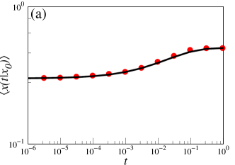
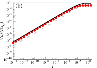
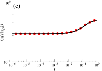
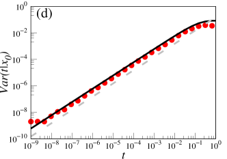
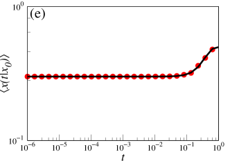
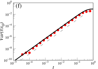
Figure 1: Temporal evolution of the mean and the variance in the scaled voter model, SDE (19), for various parameter $\gamma_{s}$ values. Red points represent the results of numerical simulations. Black (solid) lines are calculated using analytical Eq. (39), and grey dashed lines show the power-law dependence on time $\sim t^{\gamma_{s}}$. The common parameter values were set as follows: $x_{0}=0.3$ and $\varepsilon_{1}=\varepsilon_{2}=3.0$ ($b/3=1/6$). SBM anomalous diffusion exponent is different for the three cases shown: $\gamma_{s}=1/2$ for (a) and (b), $\gamma_{s}=1$ for (c) and (d), $\gamma_{s}=2$ for (e) and (e).

The mean and variance power-law scaling for the scaled voter model is very sensitive to the initial position $x_{0}$. In the case of $x_{0}>b/3$ (here $b=\frac{\varepsilon_{1}}{\varepsilon_{1}+\varepsilon_{2}}$ and $\varepsilon_{i}$ are transition rates) variance exhibits the same anomalous power-law scaling as SBM up to critical time $t_{c}$ (see Fig. 1). After critical time $t_{c}$ moments tends to their steady-state values. This is quite an unexpected result because other types of noisy voter model transformation lead to inverse power-law decay from the initial position to steady-state values for bought mean and variance for large initial value [16]. In the case of $x_{0}<b/3$ (see Fig. 2) we can observe double power-law scaling of variance (see Eq (44)). Until the influence of initial position $x_{0}$ is forgotten the variance exhibits the same anomalous scaling as SBM up to time $t_{b}$. After time $t_{b}$ the variance starts growing with the doubled exponent. For $0.5<\gamma_{s}<1$, we can observe both types of anomalous diffusion: subdiffusion transitioning into superdiffusion. For $1<\gamma_{s}<2$, the superdiffusion transitioning into superballistic motion [62]. For $0<\gamma_{s}<1$, such double power-law scaling has only been obtained in more complex models such as the Galilei variant time-fractional diffusion-advection equations [62, 63]. Numerical simulation shows that carrier-based transport through a line of cells exhibits such double power-law scaling with anomalous diffusion exponent $\gamma=0.59$ [66]. Continuous time random walk models suggest that inverse double power-law scaling the of mean current can occur in amorphous semiconductors [67]. Therefore, the ability to reproduce double power-law scaling of the variance might make our model more applicable to a variety of physical and sociophysical systems.

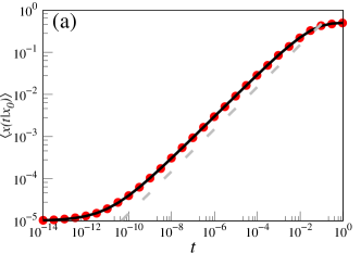
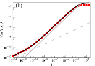
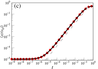
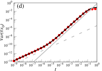
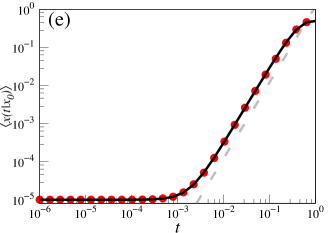
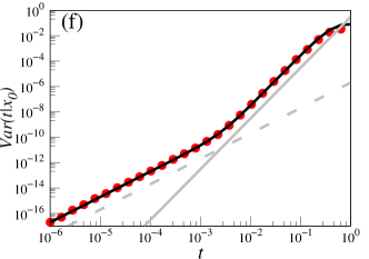
Figure 2: Temporal evolution of the mean and the variance in the scaled voter model, SDE (19), for various parameter $\gamma_{s}$ values. Red points represent the results of numerical simulations. Black (solid) lines are calculated using analytical Eq. (39), and grey lines show the power-law dependence on time $\sim t^{\gamma_{s}}$ (dashed) and $\sim t^{2\gamma_{s}}$ (solid) respectively. The common parameter values were set as follows: $x_{0}=10^{-5}$ and $\varepsilon_{1}=\varepsilon_{2}=3.0$ ($b/3=1/6$) for all pictures. SBM anomalous diffusion exponent is different for the three cases shown: $\gamma_{s}=1/2$ for (a) and (b), $\gamma_{s}=1$ for (c) and (d), $\gamma_{s}=2$ for (e) and (e).

4 First passage time distribution of the scaled voter model

In this section, we will obtain the FPTD for the special case of the noisy voter model described by SDE (18) when parameters $\varepsilon_{1}=\varepsilon_{2}=\varepsilon=1/2$. In addition, we discuss how the scaled voter model can be differentiated from other long-range memory processes using variance time dependence and obtained FPTD.

The Itô SDE (18) can be transformed into SDE with additive noise by introducing new variable $y(x)=\sqrt{2}\arcsin(\sqrt{1-x})$. By using Itô’s formula [68] we obtain SDE for a new variable $y(x(t))$

$$dy=h(t)F(y)dt-\sqrt{h(t)}dW_{t}\,.$$ (46)

The drift term time-independent part $F(y)$ is

$$F(y)=\frac{\varepsilon_{2}-\varepsilon_{1}}{\sqrt{2}}\frac{1}{\sin\big{(}\sqrt{2}y\big{)}}+\frac{\varepsilon_{1}+\varepsilon_{2}-1}{\sqrt{2}}\cot\big{(}\sqrt{2}y\big{)}.$$ (47)

Because the $x(t)$ process is bounded in interval $[0,1]$ its transformation $y(x(t))$ is bounded in $[0,\pi/\sqrt{2}]$ due to force $F(y)$.

If the condition is satisfied $\varepsilon_{1}=\varepsilon_{2}=\varepsilon$ the $F(y)$ takes a simpler form and the SDE (47) becomes

$$dy=h(t)\frac{2\varepsilon-1}{\sqrt{2}}\cot\big{(}\sqrt{2}y\big{)}dt+\sqrt{h(t)}dW_{t}\,.$$ (48)

The minus sign can be dismissed because $dW$ is statistically equivalent to $-dW$. In the case of time-independent herding behavior intensity SDE (48) has been obtained by using different nonlinear transformations [69].

In the special case when $\varepsilon=1/2$, there is no drift force and the process $y(t)$ can be described by a simpler SDE:

$$dy=\sqrt{h(t)}dW_{t}\,.$$ (49)

As in the previous section, we set the time-dependent herding behavior intensity to be a power-law function of time $h(t)=\gamma_{s}t^{\gamma_{s}-1}$. In this case, the process $y(t)$ is a special case of SBM with a diffusion coefficient equal to $D=1/2$:

$$dy=t^{\frac{\gamma_{s}-1}{2}}\sqrt{\gamma_{s}}dW_{t}\,.$$ (50)

In this special case, the scaled voter model can be interpreted as a nonlinear transformation of SBM. Because $y$ is SBM, therefore its FPTD according to Eq. (17) is

$$f_{y}(T)=\frac{|y_{0}-a_{y}|\gamma_{s}}{\sqrt{2\pi}}\frac{1}{T^{\gamma_{s}/2+1}}\exp\Bigg{(}-\frac{(y_{0}-a_{y})^{2}}{2T^{\gamma_{s}}}\Bigg{)}.$$ (51)

Here $|y_{0}-a_{y}|$ is the absolute value of the difference between initial position $y_{0}$ and threshold $a_{y}$ (absorbing boundary). In Eq. (51), an exponential term can be written in the form of $\exp(-(z/T^{-1}_{\Delta})^{\gamma_{s}})$, where $z=1/T$. Therefore for short times ($z\gg T^{-1}_{\Delta}$), we have an exponential cut-off for the short passage times. For longer passage times FPTD decays as a power-law function

$$f_{y}(T)=\frac{|y_{0}-a_{y}|\gamma_{s}}{\sqrt{2\pi}}\frac{1}{T^{\gamma_{s}/2+1}},\quad T>T_{\Delta}=2^{-\frac{1}{\gamma_{s}}}|y_{0}-a_{y}|^{\frac{2}{\gamma_{s}}}.$$ (52)

By remembering relation $y(x)=\sqrt{2}\arcsin(\sqrt{1-x})$ we obtain FPTD for the scaled voter model $x$ (for parameters $\varepsilon_{1}=\varepsilon_{2}=1/2$)

$$f_{x}(T)=\frac{\gamma_{s}\Delta_{x}}{\sqrt{2\pi}}\frac{1}{T^{\gamma_{s}/2+1}}\exp\Bigg{(}-\frac{\Delta_{x}^{2}}{2T^{\gamma_{s}}}\Bigg{)}.$$ (53)

Here $\Delta_{x}=\sqrt{2}\bigg{|}\arcsin\Big{(}\sqrt{1-x_{0}}\Big{)}-\arcsin\Big{(}\sqrt{1-a_{x}}\Big{)}\bigg{|}$ and $a_{x}$ absorption point in $x$ space.

In this section, we have shown that the noisy voter model with the time-dependent herding behavior intensity is a nonlinear transformation of SBM in an external field. By using this similarity, we have obtained an analytical approximation of FPTD. This approximation suggests that in the case of a symmetrical noisy voter model (with $\varepsilon=1/2$), FPTD has the same power-law tail as SBM FPTD. To test this prediction, we performed numerical simulations. In the numerical simulations, we use a modified next reaction method [70, 71] with an additional scaling modification, which allows us to improve simulation speed by dynamically scaling $N$ whenever greater precision is needed (see Appendix A for more details). The numerical simulations confirm that the scaled voter model exhibits FPTD with a power-law tail whose exponent is well predicted by the analytical expressions derived in this section (see Fig. 3). In addition, by using numerical simulations, we have also examined the asymmetric case, FPTD of the scaled voter model still retains the predicted power-law tail exponent. (see Fig. 4). The proposed analytical formula Eq. (53) predicts the overall shape of FPTD quite well up to large times. For large times, we see a cut-off of the power-law tail. We suspect that this deviation from the power-law might be due to reflective boundaries used in the numerical simulations or due to the influence of parameter $\varepsilon$ describing independent transition rates. To explain this phenomenon a more precise approximation is needed. It would need to take into consideration not only one absorbing boundary but the combination of the reflective and absorbing boundaries.

FPTD of the scaled noisy voter model has the same power-law tail as the SBM FPTD, but these processes can be differentiated by different power-law scaling of their MSD. The MSD for SBM is $\langle x^{2}(t)\rangle-\langle x(t)\rangle^{2}\sim t^{\gamma_{s}}$ and for the proposed noisy voter model MSD is $\langle x^{2}(t)\rangle-\langle x(t)\rangle^{2}\sim t^{2\gamma_{s}}$. When we take into consideration the initial position things can become a little bit more complicated. For $x_{0}>b/3$ variance has the same power-law scaling as MSD and processes can be easily separated from each other. For $x_{0}<b/3$ variance of the proposed model can have double power-law scaling. For shorter times, proposed model and SBM variances have identical power-law scaling. For longer times, proposed model variance starts growing with a double exponent compared to SBM. Therefore, the knowledge of both FPTD and variance lets us differentiate the considered scaled voter model from various other long-range memory processes such as SBM and fBm (fBm and SBM have identical dependence on FPTD and power-law scaling of MSD). In addition, because the FPTD can have power-law tails with other exponents than $-3/2$, this lets us differentiate our model from other nonlinear transformations of the noisy voter model [16] and Lévy flights.

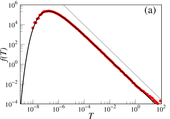
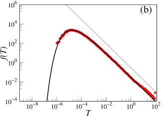
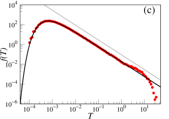
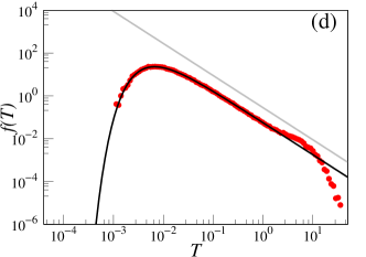
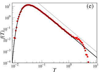
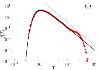
Figure 3: The first passage times $T$ distribution (FPTD) of the scaled voter model, SDE (19), for various values of the parameters $x_{0}$ and $\gamma_{s}$ values. Red points represent the results of numerical simulations. Black (solid) lines are calculated using an analytical Eq. (53), grey dashed and grey solid lines show the power-law tail of FPTD $f(t)\sim 1/t^{\beta}$ with exponent $\beta=\gamma_{s}/2+1$. The common parameter values were set as follows: $a_{x}=0$ (point of absorption) and $\varepsilon_{1}=\varepsilon_{2}=0.5$. Initial position is different for the two cases shown: $x_{0}=10^{-3}$ for (a),(c) and (e), $x_{0}=10^{-2}$ for (b),(d) and (f). SBM anomalous diffusion exponent is different for the three cases shown: $\gamma_{s}=1/2$ ($\beta=5/4$) for (a) and (b), $\gamma_{s}=1$ ($\beta=3/2$) for (c) and (d), $\gamma_{s}=2$ ($\beta=2$) for (e) and (f).

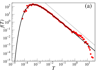
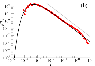
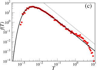
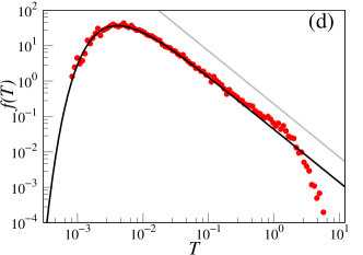
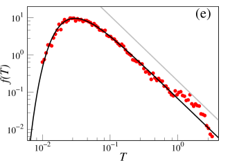
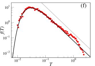
Figure 4: The first passage times $T$ distribution (FPTD) of the scaled voter model, SDE (19), for various values of the parameters $\varepsilon$ and $\gamma_{s}$. Red points represent the results of numerical simulations. Black (solid) lines are calculated using an analytical Eq. (53), and grey solid lines show the power-law tail of FPTD $f(t)\sim 1/t^{\beta}$ with exponent $\beta=\gamma_{s}/2+1$. The common parameter values were set as follows: $a_{x}=\cos^{2}(1/\sqrt{2})$ ($a_{y}=1$), $x_{0}=1/2$ ($y_{0}=\pi/\sqrt{8}$). The transition rate is different for the two cases shown: $\varepsilon=0.4$ for (a),(c) and (e), $\varepsilon=0.8$ for (b),(d) and (f). SBM anomalous diffusion exponent is different for the three cases shown: $\gamma_{s}=3/4$ ($\beta=11/8$) for (a) and (b), $\gamma_{s}=1$ ($\beta=3/2$) for (c) and (d), $\gamma_{s}=3/2$ ($\beta=7/4$) for (e) and (f).

5 Scaled voter model relation to other agent-based models

In this section, we will study how the scaled voter model relates to other ABMs and stochastic processes. We will show the noisy voter model with the time-dependent herding behavior intensity arises as a special case of other more complicated agent-based models.

In the case of $x_{0}<b/3$, the scaled voter model exhibits double power-law scaling of variance (see Eq (44)). For $0.5<\gamma_{s}<1$, we can observe both types of anomalous diffusion: the subdiffusion transitioning into superdiffusion. Similar double power-law scaling has been obtained by performing a numerical simulation of multi-state agent-based models describing carrier-based transport through a line of cells [66]. The aforementioned research and other studies [62, 63] motivated us to search for the relation between the scaled noisy voter model and multi-state ABMs. In this section, we present the simplest possible cases.

Let us start with a system of coupled SDEs

$$dn_{1}=n_{2}\left[\varepsilon_{1}\left(1-n_{1}\right)-\varepsilon_{2}n_{1}\right]dt+\sqrt{2n_{2}n_{1}\left(1-n_{1}\right)}dW_{1,t}\,.$$ (54)

$$dn_{2}=f(n_{1},n_{2})dt+g(n_{1},n_{2})dW_{2,t}\,.$$ (55)

A special case of the two dimensional stochastic process above has been used to model super-exponential financial bubbles, where the stochastic variable $n_{2}(t)=h(t)$ was interpreted as herding fluctuations driven by the Ornstein-Uhlenbeck process [20]. Therefore Eqs. (54) and (55) systems can be interpreted as noisy voter models with modulated herding behavior intensity $h(t)=n_{2}(t)$ by SDE (55). In Ref. [10] a more general case of coupled SDEs have been used to model long-range memory process such as Gaussian $1/f$ noise.

The assumption that herding behavior is time-dependent is quite common in the literature [18, 19, 20, 21]. Yet often it is assumed to be a stochastic process, while here we assume that stochastic fluctuations of variable $n_{2}$ (herding behavior intensity) can be neglected (condition $g(n_{1},n_{2})=0$ or condition $dW_{2,t}=0$ must be satisfied in SDE (55)). Also, we assume that stochastic variable $n_{2}$ is independent from $n_{1}$. These assumptions are needed to introduce long-range memory properties into our model. Our assumption might be correct when the trend in herding time dependence is much more significant than the noise.

From the aforementioned assumptions follows $f(n_{1},n_{2})=f(n_{2})$, and the SDE (55) becomes a deterministic ordinary differential equation

$$dn_{2}=f(n_{2})dt.$$ (56)

Let us consider the influence of $f(n_{2})$ on the equation system. If we set

$$f(n_{2})=(\gamma_{s}-1)\gamma_{s}^{\frac{1}{\gamma_{s}-1}}n_{2}^{1-\frac{1}{\gamma_{s}-1}},$$ (57)

then herding behavior intensity is growing according to $n_{2}(t)=\big{(}\gamma_{s}^{\frac{1}{\gamma_{s}-1}}t+n_{20}^{\frac{1}{\gamma_{s}-1}}\big{)}^{\gamma_{s}-1}$ and SDE (55) can be rearranged into

$$dn_{1}=\left[\varepsilon_{1}\left(1-n_{1}\right)-\varepsilon_{2}n_{1}\right]\big{(}\gamma_{s}^{\frac{1}{\gamma_{s}-1}}t+n_{20}^{\frac{1}{\gamma_{s}-1}}\big{)}^{\gamma_{s}-1}dt+\sqrt{2\big{(}\gamma_{s}^{\frac{1}{\gamma_{s}-1}}t+n_{20}^{\frac{1}{\gamma_{s}-1}}\big{)}^{\gamma_{s}-1}n_{1}\left(1-n_{1}\right)}dW_{1,t}\,.$$ (58)

In the above, $n_{20}$ is the initial herding behavior intensity value at the time $t=0$. If $t\gg n_{20}^{\frac{1}{\gamma_{s}-1}}/\gamma_{s}^{\frac{1}{\gamma_{s}-1}}$ or we assume that initial herding $n_{20}=0$ (at time moment $t=0$ we have only individualistic behavior), then herding behavior intensity is growing according to $n_{2}(t)=\gamma_{s}t{}^{\gamma_{s}-1}$ and SDE (58) becomes identical to SDE (19) describing the scaled voter model.

If $f(n_{2})=a(1-n_{2})$, and we set that initial herding $n_{20}=0$ (at first $t=0$ we have only individualistic behavior $n_{2}=0$) then herding behavior intensity is growing according $n_{2}=1-e^{-at}$ and

$$dn_{1}=\left[\varepsilon_{1}\left(1-n_{1}\right)-\varepsilon_{2}n_{1}\right](1-e^{-at})dt+\sqrt{2(1-e^{-at})n_{1}\left(1-n_{1}\right)}dW_{1,t}\,.$$ (59)

For small times $t\ll a^{-1}$, we obtain that stochastic variable $n_{1}$ satisfies equation

$$dn_{1}=\left[\varepsilon_{1}\left(1-n_{1}\right)-\varepsilon_{2}n_{1}\right]atdt+\sqrt{2atn_{1}\left(1-n_{1}\right)}dW_{1,t}\,.$$ (60)

If we change the timescale $t\rightarrow\frac{2t}{\sqrt{a}}$ (or by set $a=2$), we see that SDE is a special case of the scaled voter model with $\gamma_{s}=2$. SDE (60) describes a special case of the scaled voter model that could be used to approximate the short-time dynamics of the Kaizoji model [20] when the trend in herding time dependence is much more significant than the noise.

In this section, we made some suggestions on how the scaled noisy voter model might be applied to analyze other multi-state ABMs. Here, we simply assumed that only one variable is affected by the noise and the second variable behaves in a deterministic manner. Therefore the second variable can be interpreted as a mechanism generating time-dependent herding behavior intensity. In the general case, to show that two variable voter models can be approximated by using the scaled voter model one should use adiabatic or other elimination procedures of one variable [72, 73, 74]. To perform such a procedure one should know the exact form of the $g(n_{1},n_{2})$ coefficient at the diffusion term. In some cases, drift and diffusion coefficients are known [20]; in other cases they can be determined from empirical data [75]. We are planning to move in this direction for future research.

6 Conclusions

We have shown that a one-dimensional noisy voter model with a time-dependent herding behavior intensity for short times can be approximated by the CIR process with time-dependent coefficients. Additionally, general analytical expressions for the first and second moments, MSD and variance have been obtained. In the particular case when the herding behavior intensity is a power-law function (scaled voter model) of time exact moments and FPTD have been calculated. The time-dependent herding behavior intensity was chosen in such a form that the proposed scaled voter model would be a stationary process with the same variance scaling and power-law tail in FPTD as fBm. Such a tail in FPTD is unique compared to other nonlinear transformations of the voter models [11, 16]. However, the proposed model can not reproduce power-law PSD as nonlinear transformations of voter models [11, 16] (or SDEs [5]).

The proposed model has bistable steady-state distribution as bounded fBm [76, 51, 77]. We expect that in the future the combination of the scaled model and one of the proposed nonlinear transformations discussed in Ref. [16] will lead to an ABM that mimics all statistical properties of fBm.

One of the long-range memory indicators is power-law scaling of MSD. In addition, power-law scaling of MSD can be an indication of anomalous diffusion. From Eq. (41) it follows that for times smaller than $t_{c}$ the SDE (21) with power-law $h(t)$ generated signal MSD, $\langle x^{2}(t)\rangle-\langle x(t)\rangle^{2}\sim t^{2\gamma_{s}}$, scales with doubled exponent compared to SBM. Therefore we can observe anomalous diffusion for $0<\gamma_{s}<1$, and for $\gamma_{s}>1$, we can observe superballistic motion. In addition, we also have time evolution of the variance. In the case of $x_{0}>b/3$ (here $b=\frac{\varepsilon_{1}}{\varepsilon_{1}+\varepsilon_{2}}$ and $\varepsilon_{i}$ are transition rates) variance exhibits the same anomalous scaling as SBM up to critical time $t_{c}$ (see Fig. 1). After critical time $t_{c}$, moments tend to their steady-state values. In contrast, other transformations of the noisy voter model lead to inverse power-law decay of variance from the initial values to the steady-state value. [16]. In the case of $x_{0}<b/3$ and $0.5<\gamma_{s}<1$ (see Fig. 2) we can observe double power-law scaling of variance: the subdiffusion transitioning into superdiffusion (see Eq (44)). Similar double power-law scaling has only been obtained in a more complicated two-dimensional models [62, 63, 67, 66].

In Sec. 4, we have shown that the noisy voter model with the time-dependent herding behavior intensity is a nonlinear transformation of SBM in an external field. By using this similarity analytical approximation for FPTD was obtained. This approximation suggests that the scaled voter model FPTD has the same power-law tail as SBM FPTD. The numerical simulations confirm the existence of such a tail for a variety of parameter values (see Figs. 3 and 4). The derived analytical approximation, Eq. (53), predicts the overall shape of FPTD quite well up to large times. For large times, we see a cut-off of the power-law tail. The scaled noisy voter model FPTD has the same power-law tail as the SBM FPTD, but these processes can be differentiated by different power-law scaling of their MSD. The MSD for SBM is $\langle x^{2}(t)\rangle-\langle x(t)\rangle^{2}\sim t^{\gamma_{s}}$ and for the proposed noisy voter model MSD is $\langle x^{2}(t)\rangle-\langle x(t)\rangle^{2}\sim t^{2\gamma_{s}}$. Therefore the knowledge of both FPTD and variance lets us differentiate the considered scaled voter model from various other long-range memory processes such as SBM, fBm (fBm has the same FPTD and MSD as SBM, but different PSD, Lévy flights or other nonlinear transformations of the noisy voter model [16].

Author contributions

Conceptualization: R.K.; Methodology: R.K. and A.K.; Software: A.K.; Writing - Original Draft: R.K. and A.K.; Writing - Review & Editing: R.K. and A.K.; Visualization: A.K.

Appendix A Numerical simulation of the scaled voter model

In this appendix, we briefly discuss the numerical simulation method used in this paper.

Typically, to numerically simulate the noisy voter model, it is sufficient to use rejection-based simulation methods or a Gillespie method. These methods are applicable because the transition rates in the noisy voter model are not explicitly time-dependent. Here, however, we have considered the scaled voter model, which has time-dependent transition rates:

$$\pi\left(X\rightarrow X+1,t\right)= \gamma t^{\gamma-1}\left(N-X\right)\left(\varepsilon_{1}+X\right)=\gamma t^{\gamma-1}\pi_{b},$$ (61)

$$\pi\left(X\rightarrow X-1,t\right)= \gamma t^{\gamma-1}X\left(\varepsilon_{2}+\left[N-X\right]\right)=\gamma t^{\gamma-1}\pi_{d}.$$ (62)

In the above, $\pi_{b}$ and $\pi_{d}$ gather the terms which are not time-dependent. Yet some of those terms depend on $X$, which is not constant and changes as the simulation progresses, though, changes in $X$ occur during the transitions themselves.

We simulate the model with time-dependent transition rates using the modified next reaction method [70, 71], which allows the transition rates to be time-dependent. In general, the modified next reaction method requires solving multiple integral equations every time the system state is updated [70, 71]. This complication is introduced by the time-dependence of the transition rates, though, in our particular case the required integrals of the transition rates over time can be calculated analytically:

$$\int_{t}^{t+\tau}\pi\left(X\rightarrow X\pm 1,s\right)ds=\gamma\pi_{b,d}\int_{t}^{t+\tau}s^{\gamma-1}ds=\pi_{b,d}\left[\left(t+\tau\right)^{\gamma}-t^{\gamma}\right].$$ (63)

Obtaining this result allows us to avoid the numerical solution of integral equations, which speeds up the numerical simulation. See Algorithm 1 for a detailed description of the employed numerical simulation algorithm. The algorithm was implemented in C and the code was made available on GitHub (URL: https://github.com/akononovicius/anomalous-diffusion-in-nonlinear-transformations-of-the-noisy-voter-model).

Note that our implementation also includes dynamic scaling of the simulation if the system state $X$ gets close to either $0$ or $N$. Dynamic scaling of the simulation allows us to diminish the observed discretization effects while keeping the duration of the numerical simulation reasonable [16]. Otherwise, we would have to increase $N$ for simulation as a whole, which would be quite costly as the time complexity of the model is $O\left(N^{2}\right)$. Dynamic scaling allows us to increase $N$ whenever it is necessary, and otherwise run the model with lower $N$. Unlike in Ref. [16], here we have implemented both upscaling and downscaling of the simulation (overall number of particles $N$).

Appendix B First passage time distribution for scaled Brownian motion with time-dependent drift

Here we follow the works of Molini et al. [54] and Bhatia [55]. Let us start with the Fokker-Planck equation with time-dependent coefficients:

$$\frac{\partial p(x,t|x_{0},0)}{\partial t}=\mu(t)\frac{\partial p(x,t|x_{0},0)}{\partial x}+\frac{1}{2}\sigma^{2}(t)\frac{\partial^{2}p(x,t|x_{0},0)}{\partial x^{2}}.$$ (64)

Here $x=x_{0}$ is the starting point of the process and starting time is $0$. The PDF satisfies the initial condition

$$p(x,0|x_{0},0)=\delta(x-x_{0}).$$ (65)

We solve this problem with the boundary conditions. At the natural boundary, the PDF must satisfy

$$p(\infty,t|x_{0},0)=0.$$ (66)

At absorbing boundary $x=a$ ($a>0$), the PDF must satisfy the Dirichlet boundary condition:

$$p(a,t|x_{0},0)=0.$$ (67)

The survival probability $\mathbb{F}(t)$ is defined as the probability that the process trajectories are not absorbed before time $t$ and the first passage time density function $f(t)$ is given by the negative time derivative of the survival probability:

$$f(t)=-\frac{d}{dt}\mathbb{F}(t).$$ (68)

The free-space fundamental solution (Green’s function) of the Fokker-Planck equation (64) is well-known [54]:

$$p_{F}(x,t|x_{0},0)=\frac{1}{2\sqrt{\pi S(t)}}\exp\Big{(}-\frac{(x-x_{0}-M(t))^{2}}{4S(t)}\Big{)},$$ (69)

$$M(t)=\int_{0}^{t}\mu(t^{\prime})dt^{\prime}.$$ (70)

$$S(t)=\frac{1}{2}\int_{0}^{t}\sigma^{2}(t^{\prime})dt^{\prime}.$$ (71)

To solve this problem, we will use the method of images [78, 79]: the barrier at $a$ is replaced by a mirror source located at a generic point $x=m$ (mirror point), such that the solutions of Eq. (64) emanating from the original and mirror sources exactly cancel each other at the absorbing boundary Eq. (67) at each instant of time [79]. This implies the initial conditions in Eq. (65) must now be changed to [54]

$$p(x,0|x_{0},0)=\delta(x-x_{0})-e^{-\kappa}\delta(x-m),$$ (72)

where $\kappa$ determines the strength of the mirror image source. Due to the linearity of the Fokker-Planck equation (64), a solution for this partial differential equation is provided by

$$p(x,t|x_{0},0)=p_{F}(x,t|x_{0},0)-e^{-\kappa}p_{F}(x,t|m,0).$$ (73)

Here we placed an image source $e^{-\kappa}p_{F}(x,t|m,0)$ at $x=m$. Here $e^{-\kappa}$ is the strength of a mirror. From Eq. (67), it follows that equality

$$p(a,t|x_{0},0)=p_{F}(a,t|x_{0},0)-e^{-\kappa}p_{F}(a,t|m,0)=0,\$$ (74)

must be true for all times or

$$\exp\Big{(}-\frac{(a-x_{0}-M(t))^{2}}{4S(t)}\Big{)}=e^{-\kappa}\exp\Big{(}-\frac{(a-m-M(t))^{2}}{4S(t)}\Big{)}.$$ (75)

$$\frac{(a-x_{0}-M(t))^{2}}{4S(t)}=\kappa+\frac{(a-m-M(t))^{2}}{4S(t)}.$$ (76)

$$(a-x_{0}-M(t))^{2}=4S(t)\kappa+(a-m-M(t))^{2}.$$ (77)

In general Eq. (77) is nonsolvable because we have one equation and two unknown variables $m$ and $\kappa$. So, we need to make additional assumptions. We require that time-dependent mean $M(t)$ and variance $S(t)$ at initial time moment $t_{0}=0$ are also equal to zero (in the case of SBM, this is true anyway). Therefore at time moment $t=0$, Eq. (77) becomes

$$(a-x_{0})^{2}=(a-m)^{2}.$$ (78)

The aforementioned equation has two solutions:$m=x_{0}$ and $m=2a-x_{0}$. If we set $m=x_{0}$ from Eq. (77), it follows that the mirror is at the same point as the free solution. The mirror image should mirror the free solution, not copy it. If we set that $m=2a-x_{0}$, then at the initial time $0$, the free solution and its mirror image are placed at opposite sites of absorption point $a$ and with the same distance from it as a method of images requires. By putting the $m$ value into Eq. (77):

$$(a-x_{0}-M(t))^{2}=4S(t)\kappa+(x_{0}-a-M(t))^{2}.$$ (79)

$$\frac{\kappa}{x_{0}-a}=\frac{M(t)}{S(t)}.$$ (80)

For Eq. (73) to be a solution of the Fokker-Planck equation (64) parameter $\kappa$ must be a constant, therefore $M(t)$ and $S(t)$ should be chosen such as

$$\frac{M(t)}{S(t)}=q=\mathrm{const},$$ (81)

then the Fokker-Planck equation (64) solution satisfying an absorbing boundary at $x=a$ is

$$p(x,t|x_{0},0)=\frac{1}{2\sqrt{\pi S(t)}}e^{-\frac{(x-x_{0}-M(t))^{2}}{4S(t)}}-\frac{1}{2\sqrt{\pi S(t)}}e^{-(x_{0}-a)q}e^{-\frac{(x+x_{0}-2a-M(t))^{2}}{4S(t)}}.$$ (82)

The survival probability function $\mathbb{F}(x,t|x_{0},0)$, where $x=x_{0}$ represents the starting point of the diffusive process, containing the initial concentration of the distribution and $a$ is a positive lower barrier, such that $a<x_{0}$, is

$$\mathbb{F}(x,t|x_{0},0)=\int_{a}^{\infty}p(x,t|x_{0},0)dx,\quad a<x_{0}.$$ (83)

Here we show only the derivation of the FPTD if diffusion is limited to the positive domain of $x$ values $a<x_{0}$ from Eqs. (83) and (82) follows:

$$\mathbb{F}(x,t|x_{0},0)=\frac{1}{2}\Bigg{(}1+\mathrm{Erf}\Big{(}\frac{x_{0}-a+M(t)}{2\sqrt{S(t)}}\Big{)}-e^{-(x_{0}-a)q}\bigg{[}1+\mathrm{Erf}\Big{(}-\frac{x_{0}-a-M(t)}{2\sqrt{S(t)}}\Big{)}\bigg{]}\Bigg{)}.$$ (84)

FPTD $f(t)$ can be obtained by calculating the time derivative of survival probability

$$f(t)=-\frac{\partial}{\partial t}\mathbb{F}(x,t|x_{0},0).$$

To simplify the derivation, we invoked the previously made assumption that $q=M(t)/S(t)=\mathrm{const}$:

$$f_{a<x_{0}}(t)=\frac{\Big{(}x_{0}-a\Big{)}}{2\sqrt{\pi}}\frac{e^{-\frac{\big{(}x_{0}-a+M(t)\big{)}^{2}}{4S(t)}}}{S^{3/2}(t)}\frac{d}{dt}S(t),$$ (85)

To obtain the survival probability function $F(x,t|x_{0},0)$, when diffusion can occur at negative $x$ domain ( $a>x_{0}$) we need to calculate integral

$$\mathbb{F}(x,t|x_{0},0)=\int_{-\infty}^{a}p(x,t|x_{0},0)dx\quad a>x_{0}.$$ (86)

It can be shown that FPTD in such a case is

$$f_{a>x_{0}}(t)=\frac{\Big{(}a-x_{0}\Big{)}}{2\sqrt{\pi}}\frac{e^{-\frac{\big{(}x_{0}-a+M(t)\big{)}^{2}}{4S(t)}}}{S^{3/2}(t)}\frac{d}{dt}S(t).$$ (87)

By comparing $f_{a<x_{0}}(t)$ and $f_{a>x_{0}}(t)$ we see that the obtained FPTDs differ only in their sign. Therefore, without loss of generality, we can write

$$f(t)=\frac{|x_{0}-a|}{2\sqrt{\pi}}\frac{e^{-\frac{\big{(}x_{0}-a+M(t)\Big{)}^{2}}{4S(t)}}}{S^{3/2}(t)}\frac{d}{dt}S(t).$$ (88)

The case when $x_{0}=a$ is trivial if we initially set the process $x$ at the absorbing boundary: it is absorbed instantly and therefore FPTD is zero.

Now we will show that the derived general formula can reproduce the results obtained in the other works [54]. Therefore we set $\mu(t)=qAt^{\alpha}$ and $\sigma(t)=\sqrt{2A}t^{\alpha/2}$ as in Ref. [54] and put them into Eqs. (70) and (71) into (85) to obtain

$$f(t)=\frac{|x_{0}-a|(1+\alpha)^{3/2}}{2\sqrt{\pi A}}\frac{1}{t^{\frac{3+\alpha}{2}}}e^{-\frac{\big{(}qAt^{1+\alpha}+(x_{0}-a)(1+\alpha)\big{)}^{2}}{4A(1+\alpha)t^{1+\alpha}}}.$$ (89)

If we set $a=0$, FPTD coincides with the well-known result (see (Eq. (34) in Ref [54]). Parameter $q$ defines the influence of drift term $\mu(t)$; if we set $q=0$ ($\mu(t)$=0) we obtain FPTD for the drift-less case

$$f(t)=\frac{|x_{0}-a|(1+\alpha)^{3/2}}{2\sqrt{\pi A}}\frac{1}{t^{\frac{3+\alpha}{2}}}e^{-\frac{(x_{0}-a)^{2}(1+\alpha)}{4At^{1+\alpha}}}.$$ (90)

Here in the exponent we have is $(x_{0}-a)^{2}$ in Eq. (32) in Ref. [54] there is a typo: $x_{0}$ that should be $x_{0}^{2}$

Drift-less case

If we set $\mu=0$ (therefore and $M(t)=0$) then the process is described by the Fokker-Plank equation

$$\frac{\partial p(x,t|x_{0},0)}{\partial t}=\frac{1}{2}\sigma^{2}(t)\frac{\partial^{2}p(x,t|x_{0},0)}{\partial x^{2}},$$ (91)

and the method of images leads to a solution satisfying the absorbing boundary at $x=a$ (see text above)

$$p(x,t|x_{0},0)=\frac{1}{2\sqrt{\pi S(t)}}\bigg{(}e^{-\frac{(x-x_{0})^{2}}{4S(t)}}-e^{-\frac{(x+x_{0}-2a)^{2}}{4S(t)}}\bigg{)}.$$ (92)

Because there is no drift the mirror strength is 1 ($e^{-\kappa}=1,\kappa=0$). By setting $M(t)=0$ in Eq. (88), we obtain the FPTD for the process described by Eq. (91):

$$f(t)=-\frac{\partial}{\partial t}\mathbb{F}(x,t|x_{0},0)=\frac{|x_{0}-a|}{2\sqrt{\pi}}\frac{e^{-\frac{(x_{0}-a)^{2}}{4S(t)}}}{S^{3/2}(t)}\frac{d}{dt}S(t),$$ (93)

$$S(t)=\frac{1}{2}\int_{0}^{t}\sigma(t^{\prime})dt^{\prime}.$$

References

- [1] E. J. A. L. Pereira, M. F. da Silva, H. B. B. Pereira, Econophysics: Past and present, Physica A 473 (2017) 251–261. doi:10.1016/j.physa.2017.01.007.
- [2] M. Cristelli, L. Pietronero, A. Zaccaria, Critical overview of agent-based models for economics, in: F. Mallnace, H. E. Stanley (Eds.), Proceedings of the School of Physics "E. Fermi", Course CLXXVI, SIF-IOS, Bologna-Amsterdam, 2012, pp. 235–282. doi:10.3254/978-1-61499-071-0-235.
- [3] G. Teyssière, A. P. Kirman, Long memory in Economics, Springer-Verlag, Berlin, Heidelberg, 2007. doi:https://doi.org/10.1007/978-3-540-34625-8_10.
- [4] J. Beran, Y. Feng, S. Ghosh, R. Kulik, Long-memory processes probabilistic properties and statistical methods, Springer-Verlag, Berlin, Heidelberg,, 2013. doi:10.1007/978-3-642-35512-7.
- [5] R. Kazakevičius, A. Kononovicius, B. Kaulakys, V. Gontis, Understanding the nature of the long-range memory phenomenon in socioeconomic systems, Entropy 23 (2021) 1125. doi:https://doi.org/10.3390/e23091125.
- [6] V. Gontis, A. Kononovicius, S. Reimann, The class of nonlinear stochastic models as a background for the bursty behavior in financial markets, Advances in Complex Systems 15 (supp01) (2012) 1250071. doi:https://doi.org/10.1142/S0219525912500713.
- [7] R. Kazakevičius, J. Ruseckas, Anomalous diffusion in nonhomogeneous media: Power spectral density of signals generated by time-subordinated nonlinear Langevin equations, Physica A 438 (2015) 210. doi:https://doi.org/10.1016/j.physa.2015.06.047.
- [8] V. Gontis, A. Kononovicius, Burst and inter-burst duration statistics as empirical test of long-range memory in the financial markets, Physica A 483 (2017) 266–272. doi:10.1016/j.physa.2017.04.163.
- [9] V. Gontis, A. Kononovicius, Spurious memory in non-equilibrium stochastic models of imitative behavior, Entropy 19 (2017) 387. doi:10.3390/e19080387.
- [10] J. Ruseckas, R. R. Kazakevičius, B. Kaulakys, Coupled nonlinear stochastic differential equations generating arbitrary distributed observable with 1/f noise, J. Stat. Mech. 2016 (2016) 043209. doi:https://doi.org/10.1088/1742-5468/2016/04/043209.
- [11] A. Kononovicius, V. Gontis, Three state herding model of the financial markets, EPL 101 (2013) 28001. doi:10.1209/0295-5075/101/28001.
- [12] Q. Zha, G. Kou, H. Zhang, H. Liang, X. Chen, C.-C. Li, Y. Dong, Opinion dynamics in finance and business: a literature review and research opportunities, Financ. Innov. 6 (2020) 44. doi:10.1186/s40854-020-00211-3.
- [13] M. F. B. Granha, A. L. M. Vilela, C. Wang, K. P. Nelson, H. E. Stanley, Opinion dynamics in financial markets via random networks, PNAS 119 (49) (2022) e2201573119. doi:10.1073/pnas.2201573119.
- [14] G. Rangarajan, M. Ding, First passage time distribution for anomalous diffusion, Phys. Lett. A 273 (2000) 322. doi:https://doi.org/10.1016/S0375-9601(00)00518-1.
- [15] A. Kononovicius, J. Ruseckas, Continuous transition from the extensive to the non-extensive statistics in an agent-based herding model, Eur. Phys. J. B 87 (8) (2014) 169. doi:10.1140/epjb/e2014-50349-0.
- [16] R. Kazakevičius, A. Kononovicius, Anomalous diffusion in nonlinear transformations of the noisy voter model, Phys. Rev. E 103 (2021) 032154. doi:https://doi.org/10.1103/PhysRevE.103.032154.
- [17] A. Sposini, R. Metzler, G. Oshanin, Single-trajectory spectral analysis of scaled Brownian motion, New J. Phys. 21 (2019) 073043.
- [18] M. Haas, J. Krause, M. S. Paolella, S. C. Steude, Time-varying mixture GARCH models and asymmetric volatility, N. Am. J. Econ. Financ. 26 (2013) 602–623. doi:10.1016/j.najef.2013.02.024.
- [19] V. Babalos, S. Stavroyiannis, Herding, anti-herding behaviour in metal commodities futures: a novel portfolio-based approach, Appl. Econ. 47 (46) (2015) 4952–4966. doi:10.1080/00036846.2015.1039702.
- [20] T. Kaizoji, M. Leiss, A. Saichev, D. Sornette, Super-exponential endogenous bubbles in an equilibrium model of fundamentalist and chartist traders, J. Econ. Behav. Organ. 112 (2015) 289–310. doi:10.1016/j.jebo.2015.02.001.
- [21] S. Stavroyiannis, V. Babalos, Time-varying herding behavior within the Eurozone stock markets during crisis periods, Rev. Behav. Finance 12 (2) (2019) 83–96. doi:10.1108/rbf-07-2018-0069.
- [22] T. Preis, H. E. Stanley, Switching phenomena in a system with no switches, J. Stat. Phys. 138 (1-3) (2010) 431–446. doi:10.1007/s10955-009-9914-y.
- [23] A.-L. Barabasi, The origin of bursts and heavy tails in human dynamics, Nature 435 (7039) (2005) 207–211. doi:10.1038/nature03459.
-
[24]
J. E. Cox, E. I. Ingersoll, A. R. Ross,
A theory of the term structure of
interest rates, Econometrica 53 (2) (1985) 385.
doi:10.2307/1911242.
URL https://www.jstor.org/stable/1911242 - [25] J. Masoliver, Nonstationary Feller process with time-varying coefficients, Phys. Rev. E 93 (2016) 012122. doi:https://doi.org/10.1103/PhysRevE.93.012122.
- [26] C. Castellano, S. Fortunato, V. Loreto, Statistical physics of social dynamics, Rev. Mod. Phys. 81 (2009) 591–646. doi:10.1103/RevModPhys.81.591.
- [27] A. Jędrzejewski, K. Sznajd-Weron, Statistical physics of opinion formation: Is it a SPOOF?, C. R. Phys. 20 (4) (2019) 244–261. doi:10.1016/j.crhy.2019.05.002.
- [28] S. Redner, Reality inspired voter models: a mini-review, C. R. Phys. 20 (4) (2019) 275–292. doi:10.1016/j.crhy.2019.05.004.
- [29] J. Ruseckas, B. Kaulakys, V. Gontis, Herding model and 1/f noise, EPL 96 (6) (2011) 60007. doi:10.1209/0295-5075/96/60007.
- [30] A. Kononovicius, V. Gontis, Agent based reasoning for the non-linear stochastic models of long-range memory, Physica A 391 (2012) 1309.
- [31] A. Kononovicius, Empirical analysis and agent-based modeling of Lithuanian parliamentary elections, Complexity 2017 (2017) 7354642. doi:10.1155/2017/7354642.
- [32] A. Kononovicius, Compartmental voter model, J. Stat. Mech. 2019 (2019) 103402. doi:10.1088/1742-5468/ab409b.
- [33] S. Alfarano, T. Lux, F. Wagner, Time variation of higher moments in a financial market with heterogeneous agents: An analytical approach, J. Econ. Dyn. Control 32 (2008) 101–136. doi:10.1016/j.jedc.2006.12.014.
- [34] D. Braha, M. A. M. de Aguiar, Voting contagion: Modeling and analysis of a century of U.S. presidential elections, PLoS ONE 12 (5) (2017) e0177970. doi:10.1371/journal.pone.0177970.
- [35] T. Fenner, E. Kaufmann, M. Levene, G. Loizou, A multiplicative process for generating a beta-like survival function with application to the UK 2016 EU referendum results, Int. J. Mod. Phys. C 28 (11) (2017) 1750132. doi:10.1142/s0129183117501327.
- [36] S. Mori, M. Hisakado, K. Nakayama, Voter model on networks and the multivariate beta distribution, Phys. Rev. E 99 (2019) 052307. doi:10.1103/PhysRevE.99.052307.
- [37] A. Kononovicius, Supportive interactions in the noisy voter model, Chaos Soliton. Fract. 143 (2021) 110627. doi:10.1016/j.chaos.2020.110627.
- [38] N. G. van Kampen, Stochastic process in physics and chemistry, North Holland, Amsterdam, 2007.
- [39] M. Ausloos, F. Petroni, Statistical dynamics of religions and adherents, EPL 77 (3) (2007) 38002. doi:10.1209/0295-5075/77/38002.
- [40] T. Raducha, T. Gubiec, Predicting language diversity with complex networks, PLoS ONE 13 (2018) e0196593. doi:10.1371/journal.pone.0196593.
- [41] T. Raducha, M. S. Miguel, Emergence of complex structures from nonlinear interactions and noise in coevolving networks, Sci. Rep-UK 10 (1) (2020) 15660. doi:10.1038/s41598-020-72662-8.
- [42] M. Ausloos, Hagiotoponyms in France: Saint popularity, like a herding phase transition, Physica A: Statistical Mechanics and its Applications 566 (2021) 125634. doi:https://doi.org/10.1016/j.physa.2020.125634.
- [43] O. Artime, A. F. Peralta, R. Toral, J. J. Ramasco, M. San Miguel, Aging-induced continuous phase transition, Phys. Rev. E 98 (2018) 032104. doi:10.1103/PhysRevE.98.032104.
- [44] A. F. Peralta, N. Khalil, R. Toral, Ordering dynamics in the voter model with aging, Physica A 552 (2020) 122475. doi:10.1016/j.physa.2019.122475.
- [45] J. Szymański, A. Patkowski, J. Gapiński, A. Wilk, R. Hołyst, Movement of proteins in an environment crowded by surfactant micelles: Anomalous versus normal diffusion, J. Phys. Chem. B 110 (2006) 7367. doi:https://doi.org/10.1021/jp055626w.
- [46] J. Wu, M. K. Berland, Propagators and time-dependent diffusion coefficients for anomalous diffusion, Biophys. J. 95 (2008) 2049. doi:https://doi.org/10.1529/biophysj.107.121608.
- [47] F. Evers, C. Zunke, R. D. L. Hanes, J. Bewerunge, I. Ladadwa, A. Heuer, S. U. Egelhaaf, Particle dynamics in two-dimensional random-energy landscapes: Experiments and simulations, Phys. Rev. E 88 (2013) 022125.
- [48] C. Scalliet, A. Gnoli, A. Puglisi, A. Vulpiani, Cages and anomalous diffusion in vibrated dense granular media, Phys. Rev. Lett. 114 (2015) 198001.
- [49] A. Kononovicius, Noisy voter model for the anomalous diffusion of parliamentary presence, J. Stat. Mech. 2020 (6) (2020) 063405. doi:10.1088/1742-5468/ab8c39.
- [50] D. S. Vieira, J. M. E. Riveros, M. Jauregui, R. S. Mendes, Anomalous diffusion behavior in parliamentary presence, Phys. Rev. E 99 (2019) 042141. doi:10.1103/PhysRevE.99.042141.
- [51] T. Vojta, S. Halladay, S. Skinner, S. Janušonis, T. Guggenberger, R. Metzler, Reflected fractional Brownian motion in one and higher dimensions, Phys. Rev. E 102 (2020) 032108. doi:https://doi.org/10.1103/PhysRevE.102.032108.
- [52] S. C. Lim, S. V. Muniandy, Self-similar Gaussian processes for modeling anomalous diffusion, Phys. Rev. E 66 (2002) 021114. doi:https://doi.org/10.1103/PhysRevE.66.021114.
- [53] T. Guggenberger, A. Chechkin, R. Metzler, Fractional Brownian motion in superharmonic potentials and non-Boltzmann stationary distributions, J. Phys. A: Math. Theor. 54 (29) (2021) 29LT01. doi:10.1088/1751-8121/ac019b.
- [54] A. Molini, P. Talkner, G. G. Katul, A. Porporato, First passage time statistics of Brownian motion with purely time dependent drift and diffusion, Physica A 390 (2011) 1841. doi:https://doi.org/10.1016/j.physa.2011.01.024.
-
[55]
H. Bhatia, Methods for
analysis of functionals on Gaussian self similar processes, Ph.D. thesis,
University of Southern Queensland (2018).
doi:10.26192/5c0dc5eef69d8.
URL http://eprints.usq.edu.au/id/eprint/34732 - [56] A. G. Cherstvy, A. V. Chechkin, R. Metzler, Anomalous diffusion and ergodicity breaking in heterogeneous diffusion processes, New J. Phys. 15 (2013) 083039.
- [57] R. Kazakevičius, J. Ruseckas, Influence of external potentials on heterogeneous diffusion processes, Phys. Rev. E 94 (2016) 032109. doi:https://doi.org/10.1103/PhysRevE.94.032109.
- [58] M. Ding, W. Yang, Distribution of the first return time in fractional Brownian motion and its application to the study of on-off intermittency, Physical Review E 52 (1995) 207. doi:10.1103/PhysRevE.52.207.
- [59] V. V. Palyulin, G. Blackburn, M. A. Lomholt, N. W. Watkins, R. Metzler, R. Klages, A. V. Chechkin, First passage and first hitting times of Lévy flights and Lévy walks, New J. Phys. 21 (2019) 103028. doi:https://doi.org/10.1088/1367-2630/ab41bb.
- [60] A. A. Araneda, The fractional and mixed-fractional CEV model, J. Comput. Appl. Math. 363 (2020) 106. doi:https://doi.org/10.1016/j.cam.2019.06.006.
- [61] X. Gan, D. Waxman, Singular solution of the Feller diffusion equation via a spectral decomposition, Phys. Rev. E 91 (2015) 012123. doi:https://doi.org/10.1103/PhysRevE.91.012123.
- [62] R. Metzler, J. Klafter, The random walk’s guide to anomalous diffusion: a fractional dynamics approach, Phys. Rep. 339 (2000) 1.
- [63] R. Metzler, A. Compte, Generalized diffusion-advection schemes and dispersive sedimentation: A fractional approach, J. Phys. Chem. B 104 (2000) 3858.
- [64] R. Metzler, J. Klafter, The restaurant at the end of the random walk: recent developments in the description of anomalous transport by fractional dynamics, J. Phys. A: Math. Gen. 37 (2004) R161–R208.
- [65] A. G. Cherstvy, R. Metzler, Nonergodicity, fluctuations, and criticality in heterogeneous diffusion processes, Phys. Rev. E 90 (2014) 012134.
- [66] K. Kruse, A. Iomin, Superdiffusion of morphogens by receptor-mediated transport, New J. Phys. 10 (2008) 023019. doi:https://doi.org/10.1088/1367-2630/10/2/023019.
- [67] E. Barkai, Fractional fokker-planck equation solution and applications, Phys.Rev. E 63 (2001) 046118. doi:https://doi.org/10.1103/PhysRevE.63.046118.
- [68] C. W. Gardiner, Handbook of stochastic methods for Physics, Chemistry and the Natural Sciences, Springer-Verlag, Berlin, 2004.
- [69] V. Gontis, A. Kononovicius, Bessel-like birth-death process, Physica A 540 (2020) 123119. doi:10.1016/j.physa.2019.123119.
- [70] D. F. Anderson, A modified next reaction method for simulating chemical systems with time dependent propensities and delays, Chem. Phys. 127 (2007) 214107. doi:10.1063/1.2799998.
- [71] D. F. Anderson, T. G. Kurtz, Continuous time Markov chain models for chemical reaction networks, in: Design and Analysis of Biomolecular Circuits, Springer New York, 2011, pp. 3–42. doi:10.1007/978-1-4419-6766-4\_1.
- [72] J. Łuszka, Non-Markovian stochastic processes: Colored noise, Chaos 16 (2005) 026107. doi:https://doi.org/10.1063/1.1860471.
- [73] H. Hasegawa, A moment approach to non-Gaussian colored noise, Physica A 384 (2007) 241. doi:https://doi.org/10.1016/j.physa.2007.06.001.
- [74] O. Kogan, M. Khasin, B. Meerson, D. Schneider, C. R. Myers, Two-strain competition in quasineutral stochastic disease dynamics, Phys. Rev. E 90 (2014) 042149. doi:https://doi.org/10.1103/PhysRevE.90.042149.
-
[75]
J. Fan, J. Jiang, C. Zhang, Z. Zhou,
Time-dependent
diffusion models for term structure dynamics, Stat. Sinica 13 (2003)
965–992.
URL https://www3.stat.sinica.edu.tw/statistica/J13n4/j13n44/j13n44.html - [76] T. Guggenberger, T. Vojta, G. Pagnini, R. Metzler, Fractional Brownian motion in a finite interval: Correlations effect depletion or accretion zones of particles near boundaries, New J. Phys. 21 (2019) 022002. doi:https://doi.org/10.1088/1367-2630/ab075f.
- [77] A. Kononovicius, R. Kazakevičius, B. Kaulakys, Resemblance of the power-law scaling behavior of a non-Markovian and nonlinear point processes, Chaos Soliton. Fract. 162 (2022) 112508. doi:https://doi.org/10.1016/j.chaos.2022.112508.
- [78] D. R. Cox, H. D. Miller, The theory of stochastic processes, Chapman and Hall/CRC, New York, 1965. doi:https://doi.org/10.1201/9780203719152.
- [79] R. Sydney, A guide to first-passage processes, Cambridge University Press, Cambridge, 2001. doi:https://doi.org/10.1017/CBO9780511606014.