Relative Entropy-Based Constant-Envelope Beamforming for Target Detection in Large-Scale MIMO Radar With Low-Resoultion ADCs

Abstract

Hybrid digital/analog architecture and low-resolution analog-to-digital/digital-to-analog converters (ADCs /DACs) are two low-cost implementations for large-scale millimeter wave (mmWave) systems. In this paper, we investigate the problem of constant-envelope transmit beamforming for large-scale multiple-input multiple-output (MIMO) radar system, where the transmit array adopts a hybrid digital/analog architecture with a small number of RF chains and the receive array adopts a fully digital architecture with low-resolution ADCs. We derive the relative entropy between the probability density functions associated with the two test hypotheses under low-resolution ADCs. We formulate our optimization problem by maximizing the relative entropy, subject to the constant envelope and orthogonality constraints. To suboptimally solve the resultant problem, a two-stage framework is developed. In the first stage, we optimize the transmit power at the directions of the target and clutter. In the second stage, an efficient iterative algorithm based on majorization-minimization is presented to obtain the constant-envelope beamformer according to the attained transmit power. Specifically, we apply a quadratic function as the minorizer, leading to a low-complexity solution at each iteration. In addition, to further facilitate low-cost implementation of the constant-envelope beamformer, we consider the problem of one-bit beamforming design and propose an efficient iterative method based on the Nesterov-like gradient method to solve it. Numerical simulations are provided to demonstrate the effectiveness of the proposed schemes.

I Introduction

Millimeter wave (mmWave) technology has received extensive attention [1, 2, 3, 4], as a promising candidate that can settle the current challenges of bandwidth shortage and large antenna size for the vehicle radar systems. Due to the shorter wavelength at mmWave frequencies, more antennas can be placed in the same array size to achieve highly directional beamforming. This results in the large-scale concept for mmWave systems. Nevertheless, it is impractical to adopt the conventional fully digital beamforming architecture with high-resolution analog-to-digital/digital-to-analog converters (ADCs/DACs) for the large-scale antenna array. The reason is that, in conventional fully digital beamforming, each antenna requires one radio frequency (RF) chain with high-resolution ADC/DAC, which leads to prohibitive cost and power consumption for mmWave systems[5, 6, 7].

I-A Hybrid Beamforming Structure

To address the hardware limitation of conventional fully digital architecture, one potential way is to use the hybrid analog/digital scheme in which a small number of RF chains is utilized to implement the digital (baseband) beamformer and a large number of phase shifters to realize the analog beamformer. This scheme has been widely considered for mmWave communication systems [8, 9, 10, 11, 12, 13, 14]. For example, the authors in [8] propose a hybrid precoding scheme for a special case in which the number of RF chains is larger than twice that of data streams. In addition, [12] proposes an alternating method to optimize the hybrid beamformer for mmWave massive multiple-input multiple-output (MIMO) communication systems. Recently, a hybrid beamforming architecture is also considered for radar systems with sparse array[15], where the transmit and receive hybrid beamformers are jointly optimized to achieve the desired elevation-azimuth image. Additionally, the learning approach is proposed in [16] to synthesize the probing beampattern for mmWave hybrid beamforming based MIMO radar system. Further, the hybrid beamforming structure is applied in the integrated sensing and communications [17, 18].

I-B Low-resolution ADC/DAC

Another possible solution is the usage of low-resolution ADC/DAC (e.g., 1-3 bits) at each antenna, as the ADC/DAC power increases exponentially with its resolution [19]. For instance, in [20, 21, 22, 23, 24], the received signal at each antenna is directly quantized by low-resolution ADCs, and the corresponding receive digital beamforming schemes are considered without any analog beamforming. Besides, some works are devoted to investigating the quantization performance of low-resolution ADCs for MIMO systems. The authors in [25] propose the additive quantization noise model (AQNM) to fit the low-resolution quantization error for wireless systems. Using this model, the effects of the number of ADC bits on the uplink rate when considering Nakagami-$m$ fading channel and Rayleigh fading channel are analyzed in [26] and [27], respectively. In addition, the achievable rate and energy efficiency are analyzed based on the AQNM for mmWave communication system with hybrid and digital beamforming (DBF) receivers with low-resolution ADCs in [28], where the results show that in a low SNR regime, the performance of DBF with 1-2 bit ADCs outperforms HBF. Moreover, the authors in [29] extend the work in [28] to the scenario of multi-user (MU) and imperfect channel state information (CSI). More recently, the hybrid architecture with low-resolution DACs/ADCs at both transmitters and receivers are considered for mmWave communication systems in [30].

As for radar applications with low-resolution ADCs/DACs, the works mainly concentrated on DoA estimation. For instance, an algorithm is proposed in [31] to reconstruct the unquantized measurements from one-bit samples, followed by the MUSIC method to estimate the DOAs of targets. In addition, The maximum likelihood (ML) is developed in [32] for finding DoA and velocity of a target from one-bit data. Recently, the problem of DoA estimation from one-bit observations is investigated for a sparse linear array in [33]. In addition, [34] analyzes the theoretical detection gap between the one-bit and infinite-bit MIMO radars and then jointly designs the waveform and filter to achieve the theoretical performance.

Although the above works have studied the problem of parameter estimation for one-bit radar systems, the problem of transmit design with hybrid beamforming and low-resolution ADC architecture for mmWave radar detection has not yet been studied. To achieve a low cost and a low-complexity implementation for a large-scale mmWave radar system with the functionality of target detection, we explore a combination of the two promising schemes, where hybrid architecture is utilized at the transmitter, while low-resolution ADCs are adopted at the receiver.

I-C Information-theoretic Criterion for Radar Systems

On the other hand, in radar applications, the detection ability can be measured by information-theoretic quantities, including mutual information, relative entropy, etc. Recently, information-theoretic criteria have acquired extensive attention in radar systems. The pioneering work of Woodward [35] first proposes the utilization of information theory to radar receiver design. Later, the information-theoretic design criterion for a single waveform by exploiting a weighted linear sum of the mutual information between target radar signatures and the corresponding received beams is presented in [36]. Apart from these, some interesting extensions including mutual information or relative entropy-based waveform design in the presence of clutter [37, 38, 39, 40, 41, 42] emerge thereafter. Nevertheless, information-theoretic criteria is rarely considered for the large-scale mmWave radar system with low-resolution ADCs. Particularly, the resulting objective using information-theoretic criteria with low-resolution ADCs is far more complicated. The resultant problem in this work is, thus, more challenging to solve than the problem with ideal ADCs.

I-D Contributions and Notations

In this paper, we focus on transmit beamforming design via relative entropy maximization for large-scale mmWave MIMO system in the presence of (signal-dependent) clutter, the transmit array adopts a hybrid digital/analog architecture with a small number of RF chains and the receive array adopts fully digital architecture with low-resolution ADCs.

Specifically, the main contributions of this work are summarized as follows:

• For the low-cost architecture with transmit hybrid architecture and low-resolution ADCs, we derive the relative entropy between the probability density functions (PDFs) associated with the hypotheses ${\cal H}_{0}$ and ${\cal H}_{1}$ based on the AQNM, and simplify the relative entropy using some asymptotic results. With the criterion of the relative entropy maximization, we formulate the problem of transmit beamforming subject to the constant-envelope and orthogonality constraints. To the best of our knowledge, the problem of transmit design with the proposed novel architecture for mmWave radar detection has not yet been studied.

• To handle the intractable optimization problem, a two-stage optimization framework is proposed. To be more specific, we first optimize the transmit power at the directions of target and clutter, and then design the constant-envelope beamformer according to the obtained transmit power. Furthermore, in the second stage, we propose a quadratic function to minorize the quartic objective function based on the minorization-maximization (MM) framework [43, 44, 45], and obtain a closed-form solution for the quadratic programming problem at every iteration.

• To further facilitate low-cost implementation of the system, transmit beamformer implemented via one-bit phase shifters. To solve the problem of one-bit transmit beamforming, we first convert the tricky one-bit constraint into a continuous form, and develop an efficient iterative method by applying the exact penalty method (EPM) [46, 47] and Nesterov-like gradient method [48, 49].

• Representative scenarios are considered to illustrate the performance of the proposed methods for the large-scale MIMO system in terms of the relative entropy value and the detection performance in simulation.

Notation: Vectors and matrices are denoted by lower case boldface letter $\mathbf{a}$ and upper case boldface letter $\mathbf{A}$, respectively. $(\cdot)^{T}$ and $(\cdot)^{H}$ represent the transpose and conjugate transpose operators, respectively. The sets of $n$-dimensional complex-valued (real-valued) vectors and $N\times N$ complex-valued (real-valued) matrices are denoted by $\mathbb{C}^{n}$ ($\mathbb{R}^{n}$) and $\mathbb{C}^{N\times N}$ ($\mathbb{R}^{N\times N}$), respectively. $\Re\left\{\cdot\right\}$ and $\Im\left\{\cdot\right\}$ are typically reserved for the real part and the imaginary part of a complex-valued number, respectively. ${\rm vec}(\bf A)$ and ${\rm Tr}({\bf A})$ denote the vectorization and trace of $\bf A$, respectively. $\mathbf{I}_{N}$ denotes the ${N\times N}$ identity matrix. $\otimes$ and $\odot$ denote the Kronecker product and Hadamard product, respectively. The $n$-th entry of $\mathbf{a}$ is written as $a(n)$. $|\cdot|$ indicates an absolute value, cardinality, and determinant for a scalar value, a set, and a matrix depending on context.

II System Model

We consider a MIMO system in which the transmitter is equipped with $N_{t}$ antennas and $N_{\rm RF}$ RF chains. The RF chains are connected to the antennas through an analog beamformer ${\bf T}\in{\mathbb{C}^{N_{t}\times N_{\rm RF}}}$, which is realized by analog phase shifters, we have $|{\bf T}(i,j)|=\frac{1}{\sqrt{N_{t}}}$. The transmit and receive arrays are colocated, and the distance between the arrays to target/clutter is far larger than the spacing of the arrays such that a target located in the far field can be viewed as the same spatial angle relative to both of them[50, 51], and arranged as half-wavelength spaced uniform linear arrays (ULAs). While the receive system with $N_{r}$ antennas adopts a fully-digital structure, which means that each receive antenna is followed by an RF chain and a pair of ADCs for the real and imaginary parts of the received signal, as shown in Fig. 1. For reducing the hardware cost, the ADCs are considered to be few-bit.

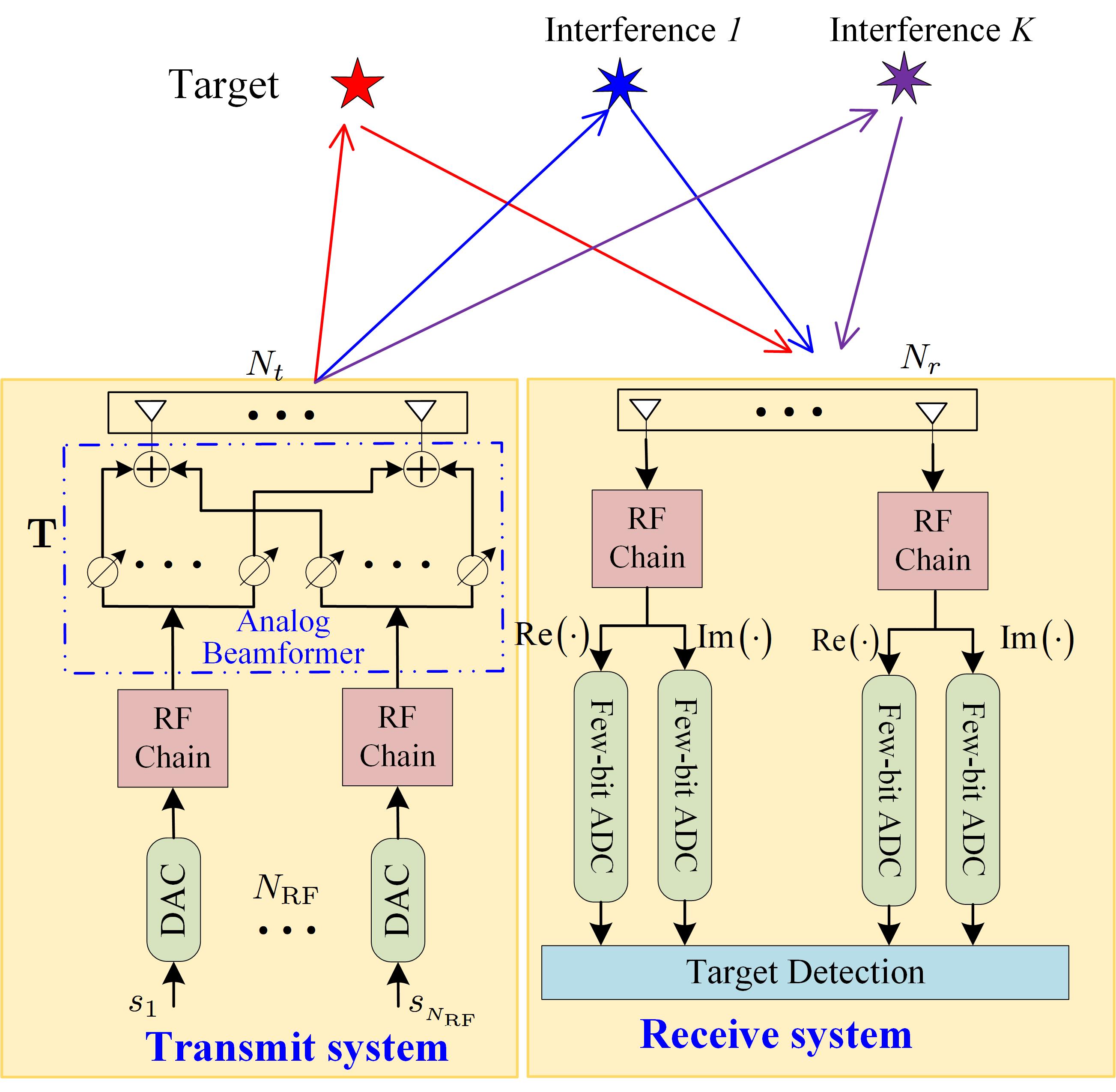
Figure 1: Overview of a large-scale MIMO system, where the transmit and receive arrays are assumed to be colocated. The transmit array adopts a hybrid digital/analog architecture and the receive array adopts few-bit ADCs.

Denote the waveform of the $n$-th RF chain at the time instant $\ell$ by $s_{n}(\ell)$. Then the transmitted waveform by the transmit array is given by

$${\bf x}(\ell)=\sum\limits_{i=1}^{{N_{{\rm{RF}}}}}{{{\bf{t}}_{i}}s_{i}(\ell)}={\bf T}{\bf s}(\ell)\in{\mathbb{C}^{N_{t}\times 1}},\ell=1,\cdots,L$$

where ${\bf s}(\ell)=[s_{1}(\ell),\cdots,s_{N_{\rm RF}}(\ell)]^{T}$, ${\bf t}_{i}$ is the $i$-th column of the matrix $\bf T$, and it can be viewed as the transmit beamspace weight corresponding to the $i$-th waveform [51, 52]. In order to obtain the waveform diversity for the MIMO radar system, the orthogonality constraint ${\bf T}^{H}{\bf T}={\bf I}_{N_{\rm RF}}$ has to be imposed [51]. Besides, $L$ is the number of samples in the duration of the transmitted waveform. Moreover, we assume that $L\geq N_{\rm RF}$, and that ${\bf s}(\ell)$ is normalized orthogonal waveform, i.e., ${\bf S}{\bf S}^{H}/L={\bf I}_{N_{\rm RF}}$, where ${\bf S}=[{\bf s}(1),\cdots,{\bf s}(L)]$.

Suppose that there exists $K$ stationary clutters in the detection area, then we can obtain the received signals at the receive antennas as

$${\bf y}(\ell)= {e^{\jmath 2\pi(\ell-1)f_{D,t}t_{s}}}{\bf H}{\bf T}{\bf s}(\ell)$$ (1)

$$+\sum\limits_{k=1}^{K}{e^{\jmath 2\pi(\ell-1)f_{D,k}t_{s}}}{\bf C}_{k}{\bf T}{\bf s}(\ell)+{\bf n}(\ell)$$

where ${\bf H}$ is the target scattering matrix, for a collocated MIMO radar, the $\bf H$ becomes a rank-one matrix, as ${\bf H}=\xi{\bf a}_{r}(\theta_{t}){\bf a}_{t}^{T}(\theta_{t})$, where $\xi$ is a random reflection coefficient, and follows ${\cal CN}(0,\sigma_{t}^{2})$, ${\bf a}_{r}(\theta)=\frac{1}{\sqrt{N_{r}}}{\left[{{\rm{1,}}\;\cdots,\;{e^{-\jmath\pi({N_{r}}-1)\sin\theta}}}\right]^{T}}$ and ${\bf a}_{t}(\theta)=\frac{1}{\sqrt{N_{t}}}\left[{{\rm{1,}}\;\cdots,\;{e^{-\jmath\pi({N_{t}}-1)\sin\theta}}}\right]^{T}$ respectively denote the receive and transmit steering vectors with $\theta_{t}$ being the direction of the target. ${\bf{C}}_{k}=\xi_{c,k}{\bf a}_{r}(\theta_{c,k}){\bf a}_{t}^{T}(\theta_{c,k})$ is the clutter response matrix of the $k$-th clutter, where $\xi_{c,k}$ and $\theta_{c,k}$ separately denote the reflection coefficient and direction of the $k$-th clutter, we also assume that $\theta_{c,1},\cdots,\theta_{c,K}$ are fixed and generated according to a uniform distribution of $[-\pi/2,\pi/2]$, and that the number and directions of clutters are known in this model. In addition, we also assume that $\left\{\xi_{c,k}\right\}$ are mutually independent and complex Gaussian random variables with zero mean and variance $\sigma_{c,k}^{2}$. $f_{D,t}$ and $f_{D,k}$ denote the Doppler frequencies of the target and $k$-th clutter, $t_{s}$ is the sample interval. ${\bf n}(l)$ is a complex Gaussian random variables with zero mean and covariance matrix $\sigma_{n}^{2}{\bf I}_{N_{r}}$.

Concatenating $L$ samples of received signals, we obtain

$${\bf Y}={\bf H}{\bf T}{\bf S}{{\bf D}_{0}}+\sum\limits_{k=1}^{K}{\bf C}_{k}{\bf T}{\bf S}{{\bf D}_{k}}+{\bf N}\in{\mathbb{C}}^{N_{r}\times L}$$ (2)

where ${\bf D}_{0}=\mathrm{Diag}([1,\cdots,e^{\jmath 2\pi(L-1)f_{D,t}}])$, ${\bf D}_{k}=\mathrm{Diag}([1,\cdots,e^{\jmath 2\pi(L-1)f_{D,k}}])$ , and ${\bf N}=[{\bf n}(1),\cdots,{\bf n}(L)]$.

For the few-bit ADCs, we adopt an additive quantization noise model (AQNM) [25, 26], which shows a reasonable accuracy for Gaussian input signal [25]. In the AQNM, the quantized output is linearized as a function of quantization bits $B$. Thus, the quantized output signal at the receiver is expressed as

$${\bf Y}_{q} ={\cal Q}({\bf Y})$$ (3)

$$\approx\alpha{\bf H}{\bf T}{\bf S}{{\bf D}_{0}}+\alpha\sum\limits_{k=1}^{K}{\bf C}_{k}{\bf T}{\bf S}{{\bf D}_{k}}+\alpha{\bf N}+{\bf N}_{q}$$

where ${\cal Q}(\cdot)$ is the element-wise quantizer, $\alpha$ is the quantization gain, defined as $\alpha=1-\beta$ with $\beta$ being the normalized mean squared quantization error. For $B=1,2,3,4,5$, the corresponding values of $\beta$ are given by 0.3634, 0.1175, 0.03454, 0.009497, and 0.002499, respectively [25]. ${\bf N}_{q}$ is the additive Gaussian quantization noise introduced by the quantization operation, and is related to the input signal ${\bf y}$ and follows the complex Gaussian distribution ${\cal CN}({\bf 0},{\bf R}_{q})$ with ${\bf R}_{q}$ being given by [25]

$${\bf R}_{q}=\alpha\beta{\rm diag}\big{(}{\bf R}_{Y}\big{)}$$ (4)

where ${\bf R}_{Y}$ is the covariance matrix of the $\bf Y$, given by

$$\begin{split}{\bf R}_{Y}=&L\sigma_{t}^{2}\phi_{t}({\bf T}){\bf a}_{r}(\theta_{t}){\bf a}_{r}^{H}(\theta_{t})\\ &+L\sum\limits_{k=1}^{K}\sigma_{c,k}^{2}\phi_{c,k}({\bf T}){\bf a}_{r}(\theta_{c,k}){\bf a}_{r}^{H}(\theta_{c,k})+L\sigma_{n}^{2}{{\bf{I}}_{{N_{r}}}}\end{split}$$ (5)

where $\phi_{t}({\bf T})\buildrel\Delta\over{=}{\bf a}_{t}^{T}(\theta_{t}){\bf T}{\bf T}^{H}{\bf a}_{t}^{*}(\theta_{t})$ and $\phi_{c,k}({\bf T})\buildrel\Delta\over{=}{\bf a}_{t}^{T}(\theta_{c,k}){\bf T}{\bf T}^{H}{\bf a}_{t}^{*}(\theta_{c,k})$ denote the transmit power for the directions of target and the $k$-th clutter, respectively.

Following [41], we establish the problem of detecting a target in the presence of observables by the following binary hypothesis test:

$$\left\{\begin{array}[]{l}{{\cal H}_{0}}:\;{{\bf{Y}}_{q}}=\alpha\sum\limits_{k=1}^{K}{\bf C}_{k}{\bf T}{\bf S}{{\bf D}_{k}}+\alpha{\bf N}+{\bf N}_{q0}\\ {{\cal H}_{1}}:\;{{\bf{Y}}_{q}}=\alpha{\bf H}{\bf T}{\bf S}{{\bf D}_{0}}+\alpha\sum\limits_{k=1}^{K}{\bf C}_{k}{\bf T}{\bf S}{{\bf D}_{k}}+\alpha{\bf N}+{\bf N}_{q1}\end{array}\right.$$ (6)

where the covariance matrices of the quantization noises ${{\bf{N}}_{q0}}$ and ${{\bf{N}}_{q1}}$ are respectively given by

$${\bf R}_{q0}=\alpha\beta L{\rm diag}\Big{(}\sum\limits_{k=1}^{K}\sigma_{c,k}^{2}\phi_{c,k}({\bf T}){\bf a}_{r}(\theta_{c,k}){\bf a}_{r}^{H}(\theta_{c,k})+\sigma_{n}^{2}{{\bf{I}}_{{N_{r}}}}\Big{)}$$ (7)

$$\quad~{}~{}=\alpha\beta L\left(\sum\limits_{k=1}^{K}\frac{\sigma_{c,k}^{2}}{N_{r}}\phi_{c,k}({\bf T})+\sigma_{n}^{2}\right){{\bf{I}}_{{N_{r}}}}$$

and

$${\bf R}_{q1}=\alpha\beta L{\rm diag}\Bigg{(}\sigma_{t}^{2}\phi_{t}({\bf T}){\bf a}_{r}(\theta_{t}){\bf a}_{r}^{H}(\theta_{t})+\sum\limits_{k=1}^{K}\sigma_{c,k}^{2}\phi_{c,k}({\bf T})$$ (8)

$$\qquad\qquad\qquad\cdot{\bf a}_{r}(\theta_{c,k}){\bf a}_{r}^{H}(\theta_{c,k})+\sigma_{n}^{2}{{\bf{I}}_{{N_{r}}}}\Bigg{)}$$

$$\quad~{}~{}=\alpha\beta L\Bigg{(}\frac{\sigma_{t}^{2}}{N_{r}}\phi_{t}({\bf T})+\sum\limits_{k=1}^{K}\frac{\sigma_{c,k}^{2}}{N_{r}}\phi_{c,k}({\bf T})+\sigma_{n}^{2}\Bigg{)}{{\bf{I}}_{{N_{r}}}}$$

In a radar system, the detection performance can be measured by the relative entropy, which is an information-theoretic metric [41]. Following [41], we select the relative entropy as our criterion in this paper. Specifically, For a target direction $\theta_{t}$ to be tested, the relative entropy between the probability density functions (PDFs) associated with the two hypothesis can be computed as

$$D(P_{0}||P_{1})$$ (9)

$$\quad=\int{{f_{0}}({{\bf{Y}}_{q}})\log}\left({\frac{{{f_{0}}({{\bf{Y}}_{q}})}}{{{f_{1}}({{\bf{Y}}_{q}})}}}\right)d{{\bf{Y}}_{q}}$$

$$\quad={\mathbb{E}}_{f_{0}}\left\{\log{f_{0}}({{\bf{Y}}_{q}})\right\}-{\mathbb{E}}_{f_{0}}\left\{\log{f_{1}}({{\bf{Y}}_{q}})\right\}$$

$$\quad=-\log\left|{\bf R}_{Y0}\right|+\log\left|{\bf R}_{Y1}\right|+{\rm Tr}\Big{(}{\bf R}_{Y1}^{-1}{\bf R}_{Y0}\Big{)}-N_{r}$$

where $f_{0}({\bf Y})$ and $f_{1}({\bf Y})$ separately denote PDFs corresponding to the test hypotheses ${\cal H}_{0}$ and ${\cal H}_{1}$, ${\bf R}_{Y0}$ and ${\bf R}_{Y1}$ are the covariance matrices of ${{\bf{Y}}_{q}}$ under the hypothesis ${\cal H}_{0}$ and ${\cal H}_{1}$, respectively, as

$${\bf R}_{Y0} =\alpha^{2}L\Big{(}\sum\limits_{k=1}^{K}\sigma_{c,k}^{2}\phi_{c,k}({\bf T}){\bf a}_{r}(\theta_{c,k}){\bf a}_{r}^{H}(\theta_{c,k})+\sigma_{n}^{2}{{\bf{I}}_{{N_{r}}}}\Big{)}$$ (10)

$$\quad+{\bf R}_{q0}$$

$$=\alpha^{2}L\Big{(}{\bf A}_{c}{\bf\Phi}_{c}({\bf T}){\bf A}_{c}^{H}+\sigma_{n}^{2}{{\bf{I}}_{{N_{r}}}}\Big{)}+{\bf R}_{q0}$$

$${\bf R}_{Y1} =\alpha^{2}L\Bigg{(}\sigma_{t}^{2}\phi_{t}({\bf T}){\bf a}_{r}(\theta_{t}){\bf a}_{r}^{H}(\theta_{t})+\sum\limits_{k=1}^{K}\sigma_{c,k}^{2}\phi_{c,k}({\bf T})$$ (11)

$$\quad~{}~{}~{}~{}~{}~{}~{}\cdot{\bf a}_{r}(\theta_{c,k}){\bf a}_{r}^{H}(\theta_{c,k})+\sigma_{n}^{2}{{\bf{I}}_{{N_{r}}}}\Bigg{)}+{\bf R}_{q1}$$

$$=\alpha^{2}L\Big{(}{\bf A}_{tc}{\bf\Phi}_{tc}({\bf T}){\bf A}_{tc}^{H}+\sigma_{n}^{2}{{\bf{I}}_{{N_{r}}}}\Big{)}+{\bf R}_{q1}$$

where ${\bf A}_{c}\buildrel\Delta\over{=}[{\bf a}_{r}(\theta_{c,1}),\cdots,{\bf a}_{r}(\theta_{c,K})]$, ${\bf A}_{tc}\buildrel\Delta\over{=}[{\bf a}_{r}(\theta_{t}),{\bf A}_{c}]$, ${\bf\Phi}_{c}({\bf T})\buildrel\Delta\over{=}{\rm diag}\big{(}[\sigma_{c,1}^{2}\phi_{c,1}({\bf T}),\cdots,\sigma_{c,K}^{2}\phi_{c,K}({\bf T})]\big{)}$ and ${\bf\Phi}_{tc}({\bf T})\buildrel\Delta\over{=}{\rm diag}\big{(}[\sigma_{t}^{2}\phi_{t}({\bf T}),\sigma_{c,1}^{2}\phi_{c,1}({\bf T}),\cdots,\sigma_{c,K}^{2}\phi_{c,K}({\bf T})]\big{)}$.

Plugging (10) and (11) into (9) yields $D(P_{0}||P_{1})$ given in (12) on the top of the next page.

$$D(P_{0}||P_{1})= \underbrace{\log\left|\alpha^{2}L\Big{(}{\bf A}_{tc}{\bf\Phi}_{tc}({\bf T}){\bf A}_{tc}^{H}+\sigma_{n}^{2}{{\bf{I}}_{{N_{r}}}}\Big{)}+{\bf R}_{q1}\right|}_{\buildrel\Delta\over{=}{\cal M}_{a}({\bf{T}})}-\underbrace{\log\left|\alpha^{2}L\Big{(}{\bf A}_{c}{\bf\Phi}_{c}({\bf T}){\bf A}_{c}^{H}+\sigma_{n}^{2}{{\bf{I}}_{{N_{r}}}}\Big{)}+{\bf R}_{q0}\right|}_{\buildrel\Delta\over{=}{\cal M}_{b}({\bf{T}})}-N_{r}$$ (12)

$$+\underbrace{{\rm Tr}\Bigg{(}\Bigg{(}\alpha^{2}L\Big{(}{\bf A}_{tc}{\bf\Phi}_{tc}({\bf T}){\bf A}_{tc}^{H}+\sigma_{n}^{2}{{\bf{I}}_{{N_{r}}}}\Big{)}+{\bf R}_{q1}\Bigg{)}^{-1}\Bigg{(}\alpha^{2}L\Big{(}{\bf A}_{c}{\bf\Phi}_{c}({\bf T}){\bf A}_{c}^{H}+\sigma_{n}^{2}{{\bf{I}}_{{N_{r}}}}\Big{)}+{\bf R}_{q0}\Bigg{)}\Bigg{)}}_{\buildrel\Delta\over{=}{\cal M}_{c}({\bf{T}})}$$

It is worthy to mention that optimizing relative entropy in (9) requires the prior knowledge of $\theta_{t}$ obtained by the cognitive paradigm. However, from practical point of view, the exact knowledge of the angle of the target is not available, and thus, it is reasonable to assume that $\theta_{t}$ is uniformly distributed random variable with $\theta_{t}\sim{\cal U}(\bar{\theta}_{t}-\Delta_{t}/2,\bar{\theta}_{t}+\Delta_{t}/2)$, where the mean $\bar{\theta}_{t}$ and the range of uncertainty $\Delta_{t}$ are assumed to be known. In such case, the averaged relative entropy can be expressed as

$${\bar{D}({P_{0}}||{P_{1}})}=\frac{1}{{{\Delta_{t}}}}\sum\limits_{{\theta_{t}}\in{\Theta_{t}}}{D({P_{0}}||{P_{1}})}$$ (13)

where the individual term ${D({P_{0}}||{P_{1}})}$ is given in (12), the set ${\Theta_{t}}$ can be obtained by taking the discretization of the set $(\bar{\theta}_{t}-\Delta_{t}/2,\bar{\theta}_{t}+\Delta_{t}/2)$, i.e.,

$${\Theta_{t}}=\left[{{{\bar{\theta}}_{t}}-\frac{{{\Delta_{t}}}}{2},\;{{\bar{\theta}}_{t}}-\frac{{{\Delta_{t}}}}{2}+{\delta_{t}},\;{{\bar{\theta}}_{t}}-\frac{{{\Delta_{t}}}}{2}+2{\delta_{t}},\cdots,{{\bar{\theta}}_{t}}+\frac{{{\Delta_{t}}}}{2}}\right]$$ (14)

with $\delta_{t}$ being the discrete spacing.

In this paper, we seek to design the constant-envelope beamformer $\bf T$ to maximize the relative entropy. Concretely, our optimization problem can be formulated as follows

$${\bf T}=\arg{\max}~{}{\bar{D}}(P_{0}||P_{1})$$ (15a)

$$\quad\qquad{\rm{s}}.{\rm{t}}.\left|{{\bf{T}}}(i,j)\right|=\frac{1}{\sqrt{N_{t}}},~{}\forall i,j$$ (15b)

$$~{}~{}~{}~{}~{}\quad\qquad{\bf{T}}^{H}{\bf{T}}={\bf I}_{N_{\rm RF}}$$ (15c)

Notice that the problem (15) is nonconvex and difficult to tackle due to the complicated objective function. Towards that end, in the following, we will propose a two-stage method to seek a suboptimal solution with low-complexity and satisfactory performance.

III The Proposed Two-Stage Method for Solving Problem (15)

In this section, we shall present the two-stage optimization framework to design the constant-envelope beamformer. To be more concretely, the proposed optimization framework includes the two steps: 1) we optimize the transmit power for the directions of target and clutters, and 2) we seek to design the constant-envelope beamformer based on the obtained transmit power.

III-A Optimization of the transmit power

Before maximizing the relative entropy with respect to the transmit power for the directions of target and clutters, the following lemma is useful.

Lemma 1.

Under the assumption that $\{\theta_{k}\}_{k=1}^{K+1}$ are independent random following a uniform distribution in $[-\pi/2,\pi/2]$, we have that ${\bf a}_{r}^{H}(\theta_{k}){\bf a}_{r}(\theta_{k})=1$ and when $N_{r}\to\infty$,

$${\mathbb{E}}\left({\bf a}_{r}^{H}(\theta_{k}){\bf a}_{r}(\theta_{l})\right)\to 0,~{}k\neq l~{}$$ (16)

$${\mathbb{V}}{\rm ar}\left({\bf a}_{r}^{H}(\theta_{k}){\bf a}_{r}(\theta_{l})\right)\to 0,k\neq l.$$

Proof:

See Appendix A. ∎

Remark 1.

Lemma 1 implies that ${\bf A}_{tc}^{H}{\bf A}_{tc}\to{\bf I}_{K+1}$, as $N_{r}\to\infty$. Fig 2 shows the average difference between ${\bf A}_{tc}^{H}{\bf A}_{tc}$ and ${\bf I}_{K+1}$ over 10000 Monte Carlo simulations for each value of $N_{r}$. We also find that the difference between ${\bf A}_{tc}^{H}{\bf A}_{tc}$ and ${\bf I}_{K+1}$ becomes small as the number of clutters $K$ decreases.

Remark 2.

Strictly speaking, Lemma 1 is applied on the mean target angle $\bar{\theta}_{t}$ and $K$ clutter angles. Since the true target angle $\theta_{t}$ is uncertain within in the set $(\bar{\theta}_{t}-\Delta_{t}/2,\bar{\theta}_{t}+\Delta_{t}/2)$, we applied the result of Lemma 1 on the slightly shifted target angle (see (14)) and the other clutter angles. Considering that $\Delta_{t}$ is a small value closing to zero, $\sin(\bar{\theta}_{t}+\delta)\approx\sin(\bar{\theta}_{t})+\epsilon$, and thereby the proof of Lemma 1 can still be valid with slight modification.

Now, we consider the upper bound of the first term of (12). Based on (8) and the identity $\left|{\bf I}+{\bf X}{\bf Y}\right|=\left|{\bf I}+{\bf Y}{\bf X}\right|$, the first term of (12) can be converted to

$${\cal M}_{a}({\bf{T}}) ={N_{r}}\log(\chi)+\log\left|{{{\bf{I}}_{K+1}}+\frac{{{\alpha^{2}}L}}{\chi}{{\bf{\Phi}}_{tc}}({\bf{T}}){\bf{A}}_{tc}^{H}{{\bf{A}}_{tc}}}\right|$$ (17)

$$\approx{N_{r}}\log(\chi)+\log\left|{{{\bf{I}}_{K+1}}+\frac{{{\alpha^{2}}L}}{\chi}{{\bf{\Phi}}_{tc}}({\bf{T}})}\right|$$

$$={N_{r}}\log(\chi)+\log\left({1+\frac{{{\alpha^{2}}L\sigma_{t}^{2}{\phi_{t}}}}{\chi}}\right)$$

$$~{}~{}~{}+\sum\limits_{k=1}^{K}\log\left({1+\frac{{{\alpha^{2}}L\sigma_{c,k}^{2}{\phi_{c,k}}}}{\chi}}\right)$$

where the second line is obtained by applying Lemma 1 and the equality is achived when $N_{r}\rightarrow\infty$, $\chi={\alpha^{2}}L\sigma_{n}^{2}+\alpha\beta L(\frac{{\sigma_{t}^{2}}}{{{N_{r}}}}{\phi_{t}}+\sum\limits_{k=1}^{K}{\frac{{\sigma_{c,k}^{2}}}{{{N_{r}}}}}{\phi_{c,k}}+\sigma_{n}^{2})$. Here, for notational simplification, $\phi_{t}({\bf T})$ and $\phi_{c,k}({\bf T})$ are separately abbreviated as $\phi_{t}$ and $\phi_{c,k}$ in the remainder of this paper.

Similarly, the second term of (12) can be rewritten as

$${\cal M}_{b}({\bf{T}}) \approx{N_{r}}\log(\varpi)+\log\left|{{{\bf{I}}_{K}}+\frac{{{\alpha^{2}}L}}{\varpi}{{\bf{\Phi}}_{c}}({\bf{T}})}\right|$$ (18)

$$={N_{r}}\log(\varpi)+\sum\limits_{k=1}^{K}{\log\left({1+\frac{{{\alpha^{2}}L\sigma_{c,k}^{2}{\phi_{c,k}}}}{\varpi}}\right)}$$

where $\varpi={\alpha^{2}}L\sigma_{n}^{2}+\alpha\beta L(\sum\limits_{k=1}^{K}{\frac{{\sigma_{c,k}^{2}}}{{{N_{r}}}}}{\phi_{c,k}}+\sigma_{n}^{2})$.

To proceed, we recast the third term of (12), based on the matrix inversion lemma, we obtain that

$$\Bigg{(}\alpha^{2}L\Big{(}{\bf A}_{tc}{\bf\Phi}_{tc}({\bf T}){\bf A}_{tc}^{H}+\sigma_{n}^{2}{{\bf{I}}_{{N_{r}}}}\Big{)}+{\bf R}_{q1}\Bigg{)}^{-1}$$ (19)

$$\qquad={{\bf{D}}^{-1}}-{{\bf{D}}^{-1}}{{\bf{A}}_{tc}}{\left({{\bf{I}}+{\alpha^{2}}L{{\bf{\Phi}}_{tc}}{\bf{A}}_{tc}^{H}{{\bf{D}}^{-1}}{{\bf{A}}_{tc}}}\right)^{-1}}$$

$$\qquad~{}~{}~{}\times\left({{\alpha^{2}}L{{\bf{\Phi}}_{tc}}}\right){\bf{A}}_{tc}^{H}{{\bf{D}}^{-1}}$$

$$\qquad=\frac{1}{\gamma}{{\bf{I}}_{{N_{r}}}}-\frac{1}{\gamma}{{\bf{A}}_{tc}}{\bf\Lambda}_{\bf T}{\bf{A}}_{tc}^{H}$$

where ${\bf D}=\gamma{\bf I}_{N_{r}}$ with $\gamma={\alpha^{2}}L\sigma_{n}^{2}+\alpha\beta L\Big{(}\frac{{\sigma_{t}^{2}}}{{{N_{r}}}}{\phi_{t}}+\sum\limits_{k=1}^{K}{\frac{{\sigma_{c,k}^{2}}}{{{N_{r}}}}}{\phi_{c,k}}+\sigma_{n}^{2}\Big{)},$ and

$${\bf\Lambda_{\bf T}}= {\rm diag}\Bigg{(}\Bigg{[}\frac{{{\alpha^{2}}L\sigma_{t}^{2}{\phi_{t}}}}{{\gamma{\rm{+}}{\alpha^{2}}L\sigma_{t}^{2}{\phi_{t}}}},\;\frac{{{\alpha^{2}}L\sigma_{c,1}^{2}{\phi_{c,1}}}}{{\gamma{\rm{+}}{\alpha^{2}}L\sigma_{c,1}^{2}{\phi_{c,1}}}},$$ (20)

$$\qquad\qquad\cdots,\frac{{{\alpha^{2}}L\sigma_{c,K}^{2}{\phi_{c,K}}}}{{\gamma{\rm{+}}{\alpha^{2}}L\sigma_{c,K}^{2}{\phi_{c,K}}}}\Bigg{]}\Bigg{)}$$

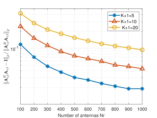
Figure 2: Errors between the ${\bf A}_{c,t}^{H}{\bf A}_{c,t}$ and ${\bf I}_{K+1}$ versus the number of receive antennas $N_{r}$ for different numbers of clutters $K$.

Define $\eta={\alpha^{2}}L\sigma_{n}^{2}+\alpha\beta L({\sum\limits_{k=1}^{K}{\frac{{\sigma_{c,k}^{2}}}{{{N_{r}}}}}{\phi_{c,k}}+\sigma_{n}^{2}})$, the third part of $D(P_{0}||P_{1})(\theta_{t})$ is rewritten in (21) on the top of the next page.

$${\cal M}_{c}({\bf{T}}) ={\rm{Tr}}\left(\frac{1}{\gamma}\Big{(}{{\bf{I}}_{{N_{r}}}}-{{\bf{A}}_{tc}}{\bf\Lambda}_{\bf T}{\bf{A}}_{tc}^{H}\Big{)}\Big{(}\eta{\bf I}_{N_{r}}+\alpha^{2}L{{\bf{A}}_{c}}{{\bf{\Phi}}_{c}}{\bf{A}}_{c}^{H}\Big{)}\right)$$ (21)

$$=\frac{\eta}{\gamma}{\rm{Tr}}\left({\bf{I}}_{N_{r}}-{{\bf{A}}_{tc}}{\bf\Lambda_{\bf T}}{\bf{A}}_{tc}^{H}\right)+\frac{{{\alpha^{2}}L}}{\gamma}{\rm{Tr}}\left({{{\bf{A}}_{c}}{{\bf{\Phi}}_{c}}{\bf{A}}_{c}^{H}}\right)-\frac{{{\alpha^{2}}L}}{\gamma}{\rm{Tr}}\left({{\bf{A}}_{tc}}{\bf\Lambda_{\bf T}}{\bf{A}}_{tc}^{H}{{{\bf{A}}_{c}}{{\bf{\Phi}}_{c}}{\bf{A}}_{c}^{H}}\right)$$

$$\approx\frac{\eta}{\gamma}N_{r}-\frac{\eta}{\gamma}{\rm{Tr}}\left({\bf\Lambda_{\bf T}}\right)+\frac{{{\alpha^{2}}L}}{\gamma}{\rm{Tr}}\left({{\bf{\Phi}}_{c}}\right)-\frac{{{\alpha^{2}}L}}{\gamma}{\rm{Tr}}\left({\bf\Lambda_{\bf T}}\left[{\begin{array}[]{*{20}{c}}{\bf{0}}\\ {{{\bf{I}}_{K}}}\end{array}}\right]{{\bf{\Phi}}_{c}}\left[{\begin{array}[]{*{20}{c}}{\bf{0}}&{{{\bf{I}}_{K}}}\end{array}}\right]\right)$$

$$=\frac{\eta}{{\gamma{\rm{+}}{\alpha^{2}}L\sigma_{t}^{2}{\phi_{t}}}}+\sum\limits_{k=1}^{K}{\frac{{\eta+{\alpha^{2}}L\sigma_{c,k}^{2}{\phi_{c,k}}}}{{\gamma+{\alpha^{2}}L\sigma_{c,k}^{2}{\phi_{c,k}}}}}+\frac{\eta}{\gamma}\left({{N_{r}}-K-1}\right)$$

Now, we want to reformulate the problem (15) into a simpler one with respect to $\big{\{}\Phi_{t},\phi_{c,1},\cdots,\phi_{c,K}\big{\}}$ for large antenna arrays, where the $\Phi_{t}$ denotes the transmit powers corresponding to possible directions of target $\Theta_{t}$ in (14). On the other hand, since ${\bf T}^{H}{\bf T}={\bf I}_{\rm RF}$, one gets

$${\bf a}_{t}^{T}(\theta_{p}){\bf T}{\bf T}^{H}{\bf a}_{t}^{*}(\theta_{p})\leq\lambda_{\max}({\bf T}{\bf T}^{H})=1,\theta_{p}\in\Theta_{P}$$

where $\Theta_{P}=\{\Theta_{t},\theta_{c,1},\cdots,\theta_{c,K}\}$, and $\lambda_{\max}(\cdot)$ denotes the maximum eigenvalue of a matrix.

With the above derivations, the problem (15) with respect to ${\Phi}_{P}\buildrel\Delta\over{=}\big{\{}\Phi_{t},\phi_{c,1},\cdots,\phi_{c,K}\big{\}}$ can be reformulated as

$${\{\phi_{p}\}}=\arg{\max}~{}g(\{\phi_{p}\})\buildrel\Delta\over{=}\sum\limits_{{\phi_{t}}\in{\Phi_{t}}}{\cal G}(\phi_{t},\{\phi_{c,k}\})$$ (22a)

$$\quad\qquad{\rm{s}}.{\rm{t}}.~{}0\leq\phi_{p}\leq 1,\forall\phi_{p}\in{\Phi}_{P}$$ (22b)

where the objective ${\cal G}(\phi_{t},\{\phi_{c,k}\})$ is defined in (23) on the top of the next page.

$${\cal G}(\phi_{t},\{\phi_{c,k}\})= \log\left|{\left({\alpha{\rm{+}}\beta}\right)\sigma_{n}^{2}+\left({\alpha+\frac{\beta}{N_{r}}}\right)\sigma_{t}^{2}{\phi_{t}}{\rm{+}}\frac{\beta}{N_{r}}\sum\limits_{k=1}^{K}{\sigma_{c,k}^{2}}{\phi_{c,k}}}\right|$$ (23)

$$+\sum\limits_{i=1}^{K}\log\Bigg{|}1+\frac{{\beta}\sigma_{t}^{2}{\phi_{t}}/{N_{r}}}{\left({\alpha+\beta}\right)\sigma_{n}^{2}+\left({\alpha+\frac{\beta}{N_{r}}}\right)\sigma_{c,i}^{2}{\phi_{c,i}}+\frac{\beta}{N_{r}}\sum\limits_{k\neq i}^{K}{\sigma_{c,k}^{2}{\phi_{c,k}}}}\Bigg{|}$$

$$+\frac{\eta}{{\gamma{\rm{+}}{\alpha^{2}}L\sigma_{t}^{2}{\phi_{t}}}}+\sum\limits_{k=1}^{K}{\frac{{\eta+{\alpha^{2}}L\sigma_{c,k}^{2}{\phi_{c,k}}}}{{\gamma{\rm{+}}{\alpha^{2}}L\sigma_{c,k}^{2}{\phi_{c,k}}}}}+\frac{\eta}{\gamma}\left({{N_{r}}-K-1}\right)$$

Notice that the complicated objective function in problem (22) makes the problem difficult to solve. Fortunately, since the constraints in problem (22) are separable, the block coordinate descent (BCD)-type method can be exploited to reach a stationary point of the problem (22) [54].

At each iteration of the BCD method, a single variable is optimized, while the remaining variables are fixed. More exactly, at the $t+1$-th iteration of the BCD method, the optimization problem with respect to $\phi_{p},\forall p$ is written as

$$\max\limits_{\phi_{p}}~{}g(\phi_{p},{\bm{\phi}}_{-p}^{(t)})~{}~{}{\rm{s}}.{\rm{t}}.~{}0\leq\phi_{p}\leq 1,\forall\phi_{p}\in{\Phi}_{P}$$ (24)

where we define ${\bm{\phi}}_{-p}^{(t)}=({\phi}_{1}^{(t)},\cdots,{\phi}_{p-1}^{(t)},{\phi}_{p+1}^{(t)},\cdots,{\phi}_{P}^{(t)})$. We note that the objective function in (24) is nonconvex and hard to deal with. Actually, its suboptimal solution can be attained by using a one-dimensional search over $(0,1)$. Concretely, we discretize the contiguous range $(0,1)$ as ${\cal K}_{p}=[0,\delta_{p},2\delta_{p},\cdots,1]$, where $\delta_{p}$ is the search interval. Thus, the suboptimal ${\phi_{p}}$ can be written as

$$\hat{\phi}_{p}=\arg\max\limits_{\phi_{p}\in{\cal K}_{p}}g\Big{(}\phi_{p},{\bm{\phi}}_{-p}^{(t)}\Big{)}.$$ (25)

Note that the main computational complexity of the BCD method is linear with the number of iterations. In each iteration, we need to update $|\Phi_{p}|$ variables successively. Thus, the total number of multiplications for solving (22) is ${\cal O}(I_{1}|\Phi_{p}|^{2}/\delta_{p})$, where $I_{1}$ is the number of iterations of the BCD. In addition, since in each update of the proposed BCD, the objective function in (22) is non-decreasing, this algorithm is able to converge to a stationary point.

In the following, we need to design the constant-envelope beamformer based on the obtained $\{\hat{\phi}_{p}\}$.

III-B Constant-Envelope Beamforming Design

In this subsection, we attempt to design the constant-envelope beamformer to make sure that ${\bf a}_{t}^{T}(\theta_{p}){\bf T}{\bf T}^{H}{\bf a}_{t}^{*}(\theta_{p}),~{}\theta_{p}\in\Theta_{P}$ approaches the obtained $\hat{\phi}(\theta_{p})$. Towards that end, the squared-error between the designed beampattern and the given beampattern is selected as the figure of merit, which is expressed as

$${\rm MSE}({\bf T})= \sum\limits_{\theta_{p}\in\Theta_{P}}{|{\bf a}_{t}^{T}(\theta_{p}){\bf T}{\bf T}^{H}{\bf a}_{t}^{*}(\theta_{p})-\hat{\phi}(\theta_{p})|^{2}}$$ (26)

Thus, our problem of the constant-envelope beamforming design with the orthogonality constraint can be formulated as

$$\min\limits_{\bf T}~{}\sum\limits_{\theta_{p}\in\Theta_{P}}{|{\bf a}_{t}^{T}(\theta_{p}){\bf T}{\bf T}^{H}{\bf a}_{t}^{*}(\theta_{p})-\hat{\phi}(\theta_{p})|^{2}}$$ (27)

$${\rm{s}}.{\rm{t}}.~{}~{}{\bf T}^{H}{\bf T}={\bf I}_{N_{\rm RF}}$$

$$\quad~{}~{}~{}\left|{{\bf{T}}}(i,j)\right|=\frac{1}{\sqrt{N_{t}}},\forall i,j$$

Problem (27) is obviously non-convex due to the orthogonality constraint. To enforce a solution which meets the orthogonality requirement, and simplify the problem, we merge the orthogonality constraint with the objective function, thus problem (27) can be relaxed as

$$\min\limits_{\bf T}{\cal Z}({\bf T})=\sum\limits_{\theta_{p}\in\Theta_{P}}{|{\bf a}_{t}^{T}(\theta_{p}){\bf T}{\bf T}^{H}{\bf a}_{t}^{*}(\theta_{p})-\hat{\phi}(\theta_{p})|^{2}}$$ (28)

$$\qquad\qquad\qquad+\varsigma\left\|{\bf T}^{H}{\bf T}-{\bf I}_{N_{\rm RF}}\right\|^{2}_{F}$$

$${\rm{s}}.{\rm{t}}.~{}\left|{{\bf{T}}}(i,j)\right|=\frac{1}{\sqrt{N_{t}}},\forall i,j$$

where $\varsigma$ is a penalty parameter for the orthogonality constraint. Nevertheless, problem (28) is still hard to solve directly due to the fact that the objective function in problem (28) is nonconvex since variables are coupled inside the Frobenius norm and squared modulus. Fortunately, the MM framework [43, 44] can be exploited to reach a stationary point of problem (28). The strategy for applying MM method is to construct an accurate majorization function, instead of minimizing the function in problem (28), the majorization function is minimized at the $\color[rgb]{0,0,0}(m)$-th iteration.

Before proceeding, the following useful Lemma is given.

Lemma 2.

For a $g({\bf X})=[{\bf u}^{T}{\bf X}{\bf X}^{H}{\bf u}^{*}]^{2}$, we have that

$$g({\bf X})\leq({{\bf{u}}^{T}}{{\bf X}^{(m)}{\bf X}^{{(m)}H}}{{\bf{u}}^{*}})\left({{\bf{u}}^{T}}{\bf X}{\bf X}^{H}{\bf{u}}^{*}\right)$$ (29)

$$-\lambda_{\rm max}\left({{\bf{u}}{{\bf{u}}^{H}}\otimes{{\bf{u}}^{*}}{{\bf{u}}^{T}}}\right)\Re\big{(}{\rm Tr}({\bf X}{\bf X}^{H}{\bf X}^{(m)}{\bf X}^{{(m)}H})\big{)}$$

$$+{\color[rgb]{0,0,0}N_{\rm RF}{{{\color[rgb]{0,0,0}\lambda_{\rm max}}\left({{\bf{u}}{{\bf{u}}^{H}}\otimes{{\bf{u}}^{*}}{{\bf{u}}^{T}}}\right)}}}$$

where ${\bf X}^{(m)}$ is the obtained $\bf X$ at the ${(m)}$-th iteration, $\lambda_{\rm max}({\bf A})$ denotes the maximum eigenvalue of $\bf A$.

Proof:

See Appendix B.∎

Based on Lemma 2 and the fact that $\lambda_{\rm max}\left({\bf{a}}_{t}({\theta_{p}}){\bf{a}}_{t}^{H}({\theta_{p}})\otimes{\bf{a}}_{t}^{*}({\theta_{p}}){\bf{a}}_{t}^{T}({\theta_{p}})\right)=1$, the following inequality holds true

$${\cal Z}({\bf T})\leq{\rm Tr}\big{(}{\bf{T}}{\bf{T}}^{H}{\bf Q}^{(m)}\big{)}+{\color[rgb]{0,0,0}\sum\limits_{\theta_{p}\in\Theta_{P}}{|\hat{\phi}(\theta_{p})|^{2}}+2\varsigma N_{\rm RF}}$$ (30)

where the matrix ${\bf Q}^{(m)}$ is defined as

$${\bf Q}^{(m)}$$ (31)

$$~{}~{}~{}=\sum\limits_{\theta_{p}\in\Theta_{P}}\left({{\bf{a}}_{t}^{T}({\theta_{p}}){\bf{T}}^{(m)}{\bf{T}}^{{(m)}H}{\bf{a}}_{t}^{*}({\theta_{p}})-2\hat{\phi}(\theta_{p})}\right){\bf{a}}_{t}^{*}({\theta_{p}})$$

$$~{}~{}~{}\cdot{\bf{a}}_{t}^{T}({\theta_{p}})-|\Theta_{P}|{\bf{T}}^{(m)}{\bf{T}}^{{(m)}H}+\varsigma\left({\bf{T}}^{(m)}{\bf{T}}^{{(m)}H}-2{\bf I}_{N_{t}}\right)$$

${\bf T}^{(m)}$ is the obtained $\bf T$ at the ${(m)}$-th iteration.

With the above derivations, the majorization problem of the constant-envelope beamforming design can be written as

$$\min\limits_{\bf T}~{}h({\bf T})={\rm Tr}\big{(}{\bf{T}}{\bf{T}}^{H}{\bf Q}^{(m)}\big{)}$$ (32)

$${\rm{s}}.{\rm{t}}.~{}\left|{{\bf{T}}}(i,j)\right|=\frac{1}{\sqrt{N_{t}}},\forall i,j$$

We note the objective function $h({\bf T})$ is a quadratic form, to which a proper majorized function can be applied again. According to the similar derivations in Appendix B, $h({\bf T})$ can be further majorized by the following function

$${\rm Tr}\big{(}{\bf{T}}{\bf{T}}^{H}{\bf Q}^{(m)}\big{)}$$ (33)

$$\quad\leq h({\bf{T}}^{(m)})+\Re\big{(}{{\bf t}^{{(m)}H}}({\bf I}_{N_{\rm RF}}\otimes{\bf Q}^{(m)})({\bf t}-{\bf t}^{(m)})\big{)}$$

$$\quad~{}~{}+\frac{{{\color[rgb]{0,0,0}\lambda_{\rm max}}({\bf I}_{N_{\rm RF}}\otimes{\bf Q}^{(m)})}}{{\rm{2}}}\left\|{\bf t}-{\bf t}^{(m)}\right\|^{2}$$

$$\quad=\Re\Big{(}{{\bf t}^{{(m)}H}}\big{(}{\bf I}_{N_{\rm RF}}\otimes{\bf Q}^{(m)}-{\color[rgb]{0,0,0}\lambda_{\rm max}}({\bf I}_{N_{\rm RF}}\otimes{\bf Q}^{(m)}){\bf I}\big{)}{\bf t}\Big{)}$$

$$\qquad+{\color[rgb]{0,0,0}N_{\rm RF}\lambda_{\rm max}({\bf I}_{N_{\rm RF}}\otimes{\bf Q}^{(m)})}$$

where ${\bf t}={\rm vec}({\bf T})$. Thus, problem (32) can be further majorized as

$$\min\limits_{\bf t}~{}\Re\Big{(}{{\bf t}^{{(m)}H}}\big{(}{\bf I}_{N_{\rm RF}}\otimes{\bf Q}^{(m)}-{\color[rgb]{0,0,0}\lambda_{\rm max}}({\bf I}_{N_{\rm RF}}\otimes{\bf Q}^{(m)}){\bf I}\big{)}{\bf t}\Big{)}$$ (34)

$${\rm{s}}.{\rm{t}}.~{}\left|{{\bf{t}}}(i)\right|=\frac{1}{\sqrt{N_{t}}},\forall i$$

Let ${{\bf{t}}}(i)=\frac{1}{\sqrt{N_{t}}}e^{\jmath\varphi_{i}}$, then the problem (34) has the following closed-form solution, as

$$\varphi_{i}=\angle{\Big{[}-\Big{(}{\bf I}_{N_{\rm RF}}\otimes{\bf Q}^{(m)}-{\color[rgb]{0,0,0}\lambda_{\rm max}}({\bf I}_{N_{\rm RF}}\otimes{\bf Q}^{(m)}){\bf I}\Big{)}{{\bf t}^{(m)}}\Big{]}_{i}}$$ (35)

Now we discuss the complexity of the MM method for designing the constant-envelope beamformer, which is linear with the iteration number. In each iteration, we need to compute the matrix ${\bf Q}^{m}$ with a complexity of ${\cal O}\left(N_{\rm RF}N_{t}^{2}\right)$, and take a SVD of ${\bf Q}^{m}$ with a complexity of ${\cal O}\left(N_{\rm RF}^{3}\right)$. Therefore, the overall complexity of the proposed MM method is ${\cal O}\left(I_{2}(N_{\rm RF}N_{t}^{2}+N_{\rm RF}^{3})\right)$, where $I_{2}$ is the number of iterations of the MM method.

Lemma 3.

Assume that the sequence of the objective values generated by Algorithm 1 is $\{\mathcal{Z}^{(m)}\}$, then the sequence is non-increasing and will converge to a local minimum.

Proof:

See Appendix C. ∎

The convergence rate of the MM method relies on the tightness of the majorization function, if the majorization function is a bad upper bound to the original one, the convergence of the MM algorithm might be much slower. To speed up its convergence, we employ the accelerated scheme based on the squared iterative method [55], which will not violate the convergence of the algorithm.

Let ${\mathbb{M}}$ denote the nonlinear updating map according to (35) during the iterations of the MM method, and express the update of ${\bf T}^{(m+1)}$ as ${\bf T}^{(m+1)}={\mathbb{M}}\left({\bf T}^{(m)}\right)$. Following the result in [55], we outline the main steps of the accelerated MM algorithm for solving the constant-envelope beamforming problem with the orthogonality constraint in Algorithm 1.

Algorithm 1 The accelerated MM method for the constant-envelope beamforming design with the orthogonality constraint

1:  Input: Initializes ${\bf T}^{(0)}$, the convergence parameter $\epsilon_{\rm AMM}>0$, $\varsigma>0$, $\varpi>1$ and $M$.

2:  Output: ${\bf T}$.

3:  Set $m=1$.

4:  repeat

5:     ${\bf Y}_{1}={\mathbb{M}}({\bf T}^{{(m-1)}})-{\bf T}^{(m-1)}$.

6:     ${\bf Y}_{2}={\mathbb{M}}\big{(}{\mathbb{M}}({\bf T}^{(m-1)})\big{)}-{\mathbb{M}}({\bf T}^{(m-1)})-{\bf Y}_{1}$.

7:     $\kappa=-\|{\bf Y}_{1}\|_{F}/\|{\bf Y}_{2}\|_{F}$.

8:     ${\bf Z}={\bf T}^{(m)}-2\kappa{\bf Y}_{1}+\kappa^{2}{\bf Y}_{2}$

9:     ${\bf T}^{(m)}=e^{\jmath\angle{\bf Z}}/\sqrt{N_{t}}$.

10:     Update $\varsigma=\varsigma\times\varpi$ every $M$ iterations.

11:     $m=m+1$.

12:  until ${\left\|{\bf T}^{(m)}-{\bf T}^{(m-1)}\right\|_{F}^{2}}\leq{\epsilon_{\rm{AMM}}}$.

IV Constant-Envelope Beamforming Design With One-Bit Phase Shifters

The part of previous section considers the infinite-resolution phase shifters are available at the transmitter. However, in order to maximally save hardware cost, in this subsection, we just consider the transmitter adopts one-bit phase shifters, i.e., ${\bf T}(i,j)\in\frac{1}{\sqrt{N_{t}}}\left\{-1,~{}1\right\},\forall i,j$, which can maximally reduce the circuit power consumption and hardware cost.

Based on the previous analysis, we design one-bit transmit beamformer with orthogonality constraint being written as

$$\min\limits_{\bf T}\sum\limits_{\theta_{p}\in\Theta_{P}}{|{\bf a}_{t}^{T}(\theta_{p}){\bf T}{\bf T}^{H}{\bf a}_{t}^{*}(\theta_{p})-\hat{\phi}_{p}|^{2}}+\varsigma\left\|{\bf T}^{T}{\bf T}-{\bf I}_{N_{\rm RF}}\right\|^{2}_{F}$$ (36)

$${\rm{s}}.{\rm{t}}.~{}{\bf T}(i,j)\in\frac{1}{\sqrt{N_{t}}}\left\{-1,~{}1\right\},\forall i,j$$

The problem (36) can be solved by an exhaustive search with exponential complexity ${\cal O}(2^{N_{t}N_{\rm RF}})$, which is not suitable for large-scale system. Alternatively, one may first obtain the solution by dropping one-bit constraint, and then projecting the resulting solution onto a one-bit set. However, this method will suffer from a large performance loss. In the following, we will apply a variational reformulation of one-bit constraint, and then propose an efficient method inspired by the idea of the exact penalty method (EPM)[46, 47] to solve the reformulated one-bit beamforming problem.

To solve the problem (36), the following proposition is useful.

Proposition 1.

One-bit set $\left\{{\bf x}\in\frac{1}{\sqrt{M}}\left\{-1,~{}1\right\}^{N}\right\}$ is equivalent to the set

$${\Psi}=\left\{({\bf x},{\bf y})|{\bf x}^{T}{\bf y}=\frac{N}{M},-\frac{1}{\sqrt{M}}\leq{\bf x}\leq\frac{1}{\sqrt{M}},{\bf y}^{T}{\bf y}\leq\frac{N}{M}\right\}.$$

Proof:

See Appendix D. ∎

Based on the Proposition 1, one-bit problem (36) can be reformulated as the following continuous one

$$\min\limits_{\bf t,~{}v}~{}\sum\limits_{\theta_{p}\in\Theta_{P}}{({\bf t}^{T}{\bf\Phi}_{p}{\bf t}-\hat{\phi}_{p})^{2}}+\varsigma\left\|{\bf T}^{T}{\bf T}-{\bf I}_{N_{\rm RF}}\right\|^{2}_{F}$$ (37)

$${\rm{s}}.{\rm{t}}.~{}-\frac{1}{\sqrt{N_{t}}}\leq{\bf t}\leq\frac{1}{\sqrt{N_{t}}}$$

$$\quad~{}~{}~{}{\bf v}^{T}{\bf v}\leq N_{\rm RF},~{}{\bf t}^{T}{\bf v}=N_{\rm RF},$$

where ${{\bf\Phi}_{p}=\Re\Big{(}{\bf I}_{N_{\rm RF}}\otimes{\bf{a}}_{t}^{*}({\theta_{p}}){\bf{a}}_{t}^{T}({\theta_{p}})\Big{)}}$ and t=vec(T). In the following, we will solve problem (37) by utilizing the EPM, which penalizes the complementary error directly by a penalty function.

More exactly, problem (37) is expressed as

$$\min\limits_{\bf t,~{}v}~{}\sum\limits_{\theta_{p}\in\Theta_{P}}{({\bf t}^{T}{\bf\Phi}_{p}{\bf t}-\hat{\phi}_{p})^{2}}+\rho(N_{\rm RF}-{\bf t}^{T}{\bf v})$$ (38)

$$\quad\qquad+\varsigma\left\|{\bf T}^{T}{\bf T}-{\bf I}_{N_{\rm RF}}\right\|^{2}_{F}$$

$${\rm{s}}.{\rm{t}}.~{}-\frac{1}{\sqrt{N_{t}}}\leq{\bf t}\leq\frac{1}{\sqrt{N_{t}}},~{}{\bf v}^{T}{\bf v}\leq N_{\rm RF}$$

where $\rho$ is the penalty parameter for the constraint ${\bf t}^{T}{\bf v}=N_{\rm RF}$. Note that $N_{\rm RF}-{\bf t}^{T}{\bf v}\geq 0$ always holds for any feasible $({\bf t},{\bf v})$. The selection scheme of $\rho$ is similar to that of $\varsigma$. To solve the problem (38) with a fixed $\rho$, we can first obtain the closed-form solution of $\bf v$, which is dependent on $\bf t$, and substituted it into problem (38), and update $\bf t$ with aid of the gradient method.

Specifically, for an arbitrary ${\bf t}$, the $\bf v$ is updated by solving

$$\min\limits_{\bf v}~{}-{\bf t}^{T}{\bf v},~{}~{}{\rm{s}}.{\rm{t}}.~{}~{}~{}{\bf v}^{T}{\bf v}\leq N_{\rm RF}$$ (39)

whose closed-form solution is ${\bf v}={{\sqrt{{N_{{\rm{RF}}}}}{{\bf{t}}}}}/{{\left\|{{{\bf{t}}}}\right\|}}$.

Substituting ${\bf v}={{\sqrt{{N_{{\rm{RF}}}}}{{\bf{t}}}}}/{{\left\|{{{\bf{t}}}}\right\|}}$ into problem (38), problem (38) reduces to a minimization problem with respect to $\bf t$, as

$$\min\limits_{\bf t}~{}{\cal F}_{\rho}({\bf t})=\sum\limits_{\theta_{p}\in\Theta_{P}}{({\bf t}^{T}{\bf\Phi}_{p}{\bf t}-\hat{\phi}_{p})^{2}}+\rho(N_{\rm RF}-\sqrt{N_{\rm RF}}\|{\bf t}\|)$$ (40)

$$\quad\qquad\qquad\quad\quad+\varsigma\left\|{\bf T}^{T}{\bf T}-{\bf I}_{N_{\rm RF}}\right\|^{2}_{F}$$

$${\rm{s}}.{\rm{t}}.~{}-\frac{1}{\sqrt{N_{t}}}\leq{\bf t}\leq\frac{1}{\sqrt{N_{t}}}$$

The problem (40) is a large-scale smooth problem with a compact constraint, to take advantage of the structure of the constraint, we develop an accelerated proximal gradient method, i.e., Nesterov-like gradient method [48, 49], to handle it. To be more specific, at the $\color[rgb]{0,0,0}(p)$-th iteration, the Nesterov-like gradient method updates $\bf t$ as follows

$${\bm{w}}^{(p)}={\bf t}^{(p)}+\frac{\tau^{(p-1)}}{\tau^{(p+1}}\Big{(}{\bf t}^{(p)}-{\bf t}^{(p-1)}\Big{)}$$ (41a)

$${\bf t}^{(p+1)}=\prod\nolimits_{-\frac{1}{{\sqrt{{N_{t}}}}}\leq{\bf{t}}\leq\frac{1}{{\sqrt{{N_{t}}}}}}\Big{(}{\bm{w}}^{(p)}-\mu^{(p)}\nabla_{\bf t}{\cal F}_{\rho}({\bf t})\Big{)}$$ (41b)

where $\tau^{(p+1)}=\frac{{1+\sqrt{1+4{{\left({{\tau^{(p)}}}\right)}^{2}}}}}{2}$, $\mu^{(p)}$ is a step size which can be determined by a backtracking line search [56], $\prod\nolimits_{{\cal S}}(\cdot)$ is the projection operator onto set $\cal S$. Additionally, as derived in Appendix E, the $(j-1)\times N_{t}+i$th element of $\nabla_{\bf t}{\cal F}_{\rho}({\bf t})$ is given by

$$[\nabla_{\bf t}{\cal F}_{\rho}({\bf t})]_{(j-1)\times N_{t}+i}=$$ (42)

$$\sum\limits_{\theta_{p}\in\Theta_{P}}{({{\bf{t}}^{T}}{{\bf{\Phi}}_{p}}{\bf{t}}-{{\hat{\phi}}_{p}}){{\bf{\Phi}}_{p,((j-1){N_{t}}+i):}}{\bf{t}}}-\frac{\rho\sqrt{N_{\rm RF}}}{\|{\bf t}\|}t_{(j-1){N_{t}}+i}$$

$$~{}~{}+\varsigma\Bigg{(}4T_{i,j}^{3}+4T_{i,j}\left(\big{[}{\overline{\bf{T}}}_{i,j}^{T}{\overline{\bf{T}}}_{i,j}-{\bf I}_{N_{\rm RF}}\big{]}_{j,j}+\big{[}{\overline{\bf{T}}}_{i,j}{\overline{\bf{T}}}_{i,j}^{T}\big{]}_{i,i}\right)$$

$$~{}~{}~{}~{}~{}~{}~{}~{}~{}~{}+4\big{[}\overline{\bf{T}}_{i,j}\big{(}{\overline{\bf{T}}}_{i,j}^{T}{\overline{\bf{T}}}_{i,j}-{\bf I}_{N_{\rm RF}}\big{)}\big{]}_{i,j}\Bigg{)},$$

$$\qquad\quad j=1,\cdots,N_{\rm RF};i=1,\cdots,N_{t}$$

where ${{{\bf{\Phi}}_{p,((j-1){N_{t}}+i):}}}$ denotes the $(j-1){N_{t}}+i$-th row of the matrix ${\bf{\Phi}}_{p}$, $t_{(j-1){N_{t}}+i}$ stands for the $(j-1){N_{t}}+i$-th entry of the vector ${\bf t}$, and ${\overline{\bf{T}}}_{i,j}$ is the matrix $\bf{T}$ whose $(i,j)$-th entry is zeroed.

We note that the Nesterov-like gradient method provides a faster convergence rate than that of the traditional gradient method [48, 49].

Based on the above analysis, the Nesterov-like gradient method for one-bit beamforming design is summarized in Algorithm 2.

The main complexity of the proposed method for one-bit transmit beamforming design is caused by computing the gradient of ${\cal F}_{\rho}({\bf t})$, i.e., $\nabla_{\bf t}{\cal F}_{\rho}({\bf t})$, which requires a complexity of ${\cal O}\left(|\Phi_{p}|N_{t}^{2}N_{\rm RF}^{2}\right)$. Therefore, the overall complexity of one-bit beamforming design is ${\cal O}\left({I}_{3}|\Phi_{p}|N_{t}^{2}N_{\rm RF}^{2}\right)$, where $I_{3}$ is the number of iterations of the Nesterov-like gradient method.

Algorithm 2 The Nesterov-like gradient method for designing one-bit beamformer.

1:  Input: Initializes ${\bf t}^{(0)},\tau^{(0)}$, the convergence parameter $\epsilon_{\rm EPM}>0$, $\varsigma,\rho>0$, $\varpi,\varrho>1$ and $M,N$.

2:  Output: ${\bf t}$.

3:  Set $p=0$.

4:  repeat

5:     Compute ${\tau}^{{(p+1)}}=\tau^{{(p+1)}}=\frac{{1+\sqrt{1+4{{\left({{\tau^{(p)}}}\right)}^{2}}}}}{2}$.

6:     Obtain $\mu^{(p)}$ by a backtracking line search.

7:     Compute ${\bm{w}}^{(p)}={\bf t}^{(p)}+\frac{\tau^{(p)}-1}{\tau^{(p+1)}}\Big{(}{\bf t}^{(p)}-{\bf t}^{(p-1)}\Big{)}$.

8:     Update ${\bf t}^{(p+1)}=\prod\nolimits_{-\frac{1}{{\sqrt{{N_{t}}}}}\leq{\bf{t}}\leq\frac{1}{{\sqrt{{N_{t}}}}}}\Big{(}{\bm{w}}^{(p)}-\mu^{(p)}\nabla_{\bf t}{\cal F}_{\rho}({\bf t})\Big{)}$.

9:     Update $\varsigma=\varsigma\times\varpi$ every $M$ iterations.

10:     Update $\rho=\rho\times\varrho$ every $N$ iterations.

11:     Compute ${\bf g}^{(p+1)}=\nabla_{\bf t}{\cal F}_{\rho}({\bf t}^{(p+1)})$.

12:     $p=p+1$.

13:  until ${\left\|{\bf g}^{(p)}\right\|}\leq{\epsilon_{\rm{EPM}}}$.

V Numerical Simulations

In this section, several sets of numerical simulations are presented to assess the performance of the proposed beamforming designs. We first evaluate the performance of the constant-envelope beamformer with infinite-resolution phase shifters, and then the beamforming design with one-bit phase shifters is considered.

Unless otherwise specified, in all simulations, we consider that the transmitter and receiver are ULAs of $N_{t}=128$ and $N_{r}=128$, respectively. The transmit array is equipped with $N_{\rm RF}=8$ RF chains. The transmit waveform $\bf S$ is chosen to be orthogonal LFM [57], whose code length is $L=16$. We assume the target is located at $\theta_{t}=0^{\circ}$ with the uncertainty of ${\Delta_{t}=2^{\circ}}$, and the variance of its reflection coefficient is $\sigma_{t}^{2}=0$ dB. In addition, we assume that the scattering strength is $\sigma^{2}_{c,k}=30$ dB (for all $k$). The directions of the clutter considered in our simulations are listed in the following table.

TABLE I: The parameter settings of the clutters in simulations.

	The directions of the clutters
$K=5$	$-31.0^{\circ},-3.3^{\circ},28.7^{\circ},-73.7^{\circ},69.1^{\circ}$
$K=10$	$-15.3^{\circ},22.0^{\circ},59.9^{\circ},-47.6^{\circ},-75.4^{\circ},78.9^{\circ},-11.4^{\circ},61.9^{\circ},34.1^{\circ},-64.7^{\circ}$
$K=15$	$-40.4^{\circ},-12.1^{\circ},24.6^{\circ},-16.7^{\circ},-72.0^{\circ},30.4^{\circ},47.5^{\circ},75.8^{\circ},-86.2^{\circ},-12.7^{\circ},-79^{\circ},$
	$-81.9^{\circ},54.4^{\circ},22.9^{\circ},3.6^{\circ}$
$K=20$	$34.1^{\circ},-4.3^{\circ},-9.0^{\circ},-42.6^{\circ},39.5^{\circ},89.6^{\circ},-12.4^{\circ},-23.1^{\circ},25.2^{\circ},8.7^{\circ},45.1^{\circ},$
	$-82.9^{\circ},34.1^{\circ},-6.2^{\circ},15.2^{\circ},2.4^{\circ},22.5^{\circ},-18.7^{\circ},-33.6^{\circ},32.3^{\circ}$

The variance of the Gaussian white noise is $\sigma_{n}^{2}=0$ dB. As to the stop criteria of the proposed algorithms, we set the tolerance $\epsilon=10^{-4}$.

In all simulations, we denote the MM method with acceleration and the general MM without acceleration as “AMM”, and “MM”, respectively.

V-A Constant-Envelope beamforming with infinite-resolution phase shifters

In this subsection, we examine the performance of the proposed beamforming method with infinite-resolution phase shifters.

Example 1: Fig. 3 analyzes the convergence performance of the MM method with acceleration for solving problem (26) by considering one-bit ADCs adopted at the receiver, $N_{t}=128$, $N_{\rm RF}=8$ and $N_{r}=128$. We consider a scenario where the $10$ clutter scatterers, their directions are randomly generated with a uniform distribution over $[-90^{\circ},90^{\circ}]$, to be specific, the considered directions of clutters are listed in Tab. I. Fig. 3(a) and Fig. 3(b) respectively reveal the beampattern MSE (i.e., ${\rm MSE}({\bf T})$ in Eq. (26)) and relative entropy of the designed beamformer by using the AMM method, for comparison purpose, the general MM, BCD and the two-stage method in [58] that firstly obtains the optimal digital beamformer by dropping the nonconvex constant-envelope constraint, and then projects the optimal digital beamformer onto the constant modulus set are also considered. The result shows that the convergence rate of the general MM is rather slower than that of the AMM, this result agrees with that in [55]. Moreover, the proposed AMM method remarkably outperforms the MM, BCD and the two-stage method in [58] in terms of the relative entropy performance. The corresponding relative entropy, computational complexity per iteration and the total iterations number as well as the consumed time per iteration are given in Table II. The results in Table II also show that the AMM method performs better than the other two methods with respect to the relative entropy and computational efficiency.

TABLE II: Property analysis of various methods

	AMM	MM	BCD	Method in [54]
relative entropy	0.3833	0.2439	0.3071	0.2713
computational complexity	${\cal O}(N_{\rm RF}N_{t}^{2}+N_{\rm RF}^{3})$	${\cal O}(N_{\rm RF}N_{t}^{2}+N_{\rm RF}^{3})$	${\cal O}(N_{\rm RF}^{2}N_{t}^{3}K+N_{t}^{3}N_{\rm RF}K^{2})$	${\cal O}(N_{\rm RF}N_{t}^{2}K+N_{\rm RF}K^{2})$
total iterations number	1500	1500	500	500
consumed time per iteration	0.0563	0.0378	3.241	0.5062

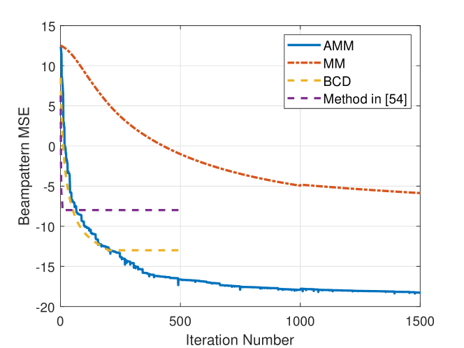
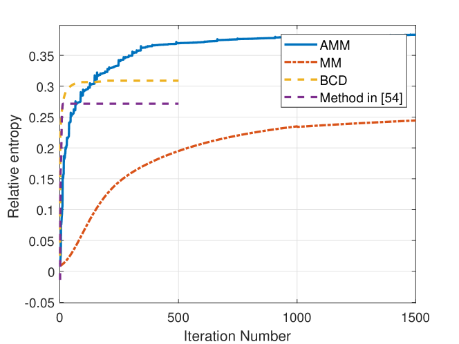
Figure 3: The convergence performance of the proposed constant-envelope beamforming method. (a) The beampattern MSE of the designed constant-envelope beamformers versus iteration number, (b) the relative entropy of the designed constant-envelope beamformers versus iteration number.

Example 2: In example 2, we have evaluated the relative entropy value of the designed scheme for different numbers of ADC bits and RF chains. The remaining parameters are the same as example 1. Fig. 4 shows the relative entropy value versus the number of RF chains for different ADC bits. The results show that the larger the number of the RF chains, the better the relative entropy can be achieved. This is because more RF chains mean more degrees of freedom (DoFs) can be applied in the design stage. Moreover, as the number of ADC bits increase, the improvement of the relative entropy value becomes less and less apparent. Specifically, when the ADC bit number is larger than 3, the performance gap with the ideal ADCs are very small. This suggests that there is no need to adopt the high resolution ADCs in the receive system, and therefore, the hardware cost can be significantly reduced in MIMO radar system. The probabilities of detection associated with the designed beamformers for different ADC bits with $N_{\rm RF}=8$ is plotted in Fig. 5, where the probability of false alarm $P_{\rm fa}=10^{-4}$, the number of Monte-Carlo trails is $10^{6}$ and the SNR is defined as ${\rm SNR}=\sigma_{t}^{2}/\sigma_{n}^{2}$. The result shows that, as the number of ADC bits increase, and the probability of detection will be better and better.

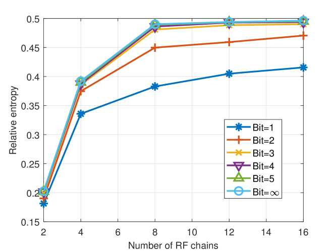
Figure 4: The relative entropy values versus the number of RF chains for different numbers of ADC bits $\rm Bit$.

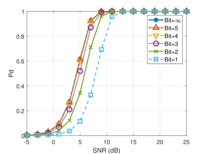
Figure 5: The detection performance versus SNR for different quantization levels $\rm Bit$. $P_{\rm fa}=10^{-4}$.

Fig. 6 displays the probabilities of detection of the designed scheme for different numbers of RF chains with one-bit ADCs, this result shows that the probability of detection the beamformer with $N_{\rm RF}=4$ is obviously better than that of the beamformer with $N_{\rm RF}=2$, but this improvement becomes marginal when the $N_{\rm RF}$ continues to increase. Particularly, the beamformers with $N_{\rm RF}=16$ and $N_{\rm RF}=32$ have almost identical performance.

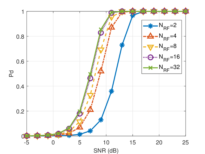
Figure 6: The detection performance versus SNR for different numbers of the RF chains. $P_{\rm fa}=10^{-4}$, ${\rm Bit}=1$.

Example 3: In this example, the effect of the number of clutters on the performance of the proposed method is assessed in Fig. 8. To be specific, we consider the five cases, i.e., $K=0$ (no clutter), $K=5$, $K=10$, $K=15$, $K=20$. The specific directions of clutter of the considered case are listed in Tab. 1. The remaining parameters are the same as example 1. Fig. 7 plots the relative entropy versus numbers of receive antennas $N_{r}$ a different number of clutters $K$. Note that the curve of $K=0$ provides the upper bound for our design. The result shows that for a fixed $N_{r}$, the performance degradation increases with the increasing of the number of clutters increases. Moreover, we find that as the number of clutters decreases, the improvement provided by adding the number of receive antennas $N_{r}$ becomes more and more marginal. Particularly, when $K=0$, the relative entropy value does not decrease with increasing $N_{r}$. The reason lies in that the asymptotic error ${\bf A}_{tc}^{H}{\bf A}_{tc}\to{\bf I}_{K+1}$ in Lemma 1 becomes smaller as the number of receive antennas increases, and the performance loss caused by our model is smaller. Fig. 7(b) shows the detection performance versus SNR value for $K=10$, $N_{\rm RF}=8$ and $P_{\rm fa}=10^{-4}$ when considering $N_{t}=N_{r}=128$. The result agrees with our expectation.

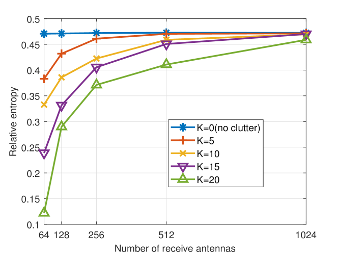
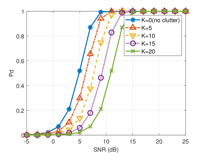
Figure 7: Performance of the proposed design for a different number of clutters. (a) The relative entropy values versus the number of receive antennas. (b) The detection performance versus SNR value for $P_{\rm fa}=10^{-4}$, $N_{t}=N_{r}=128$.

Example 4: Fig. 8 shows the relative entropy as a function of the number of RF chains for different uncertainties on $\theta_{t}$, i.e., $\Delta_{t}$, when considering $K=10$. It is not surprising to find that the larger inaccuracies in the knowledge of $\theta_{t}$, the greater the relative entropy loss will be. Additionally, we also observe that as the number of RF chains increases, the relative entropy values become larger and larger.

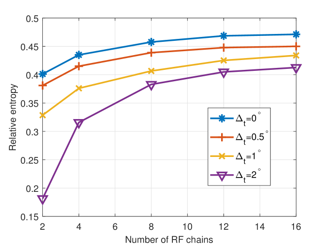
Figure 8: The relative entropy values versus the number of RF chains when considering different uncertainties on $\theta_{t}$.

V-B Transmit beamforming with one-bit phase shifters

In this subsection, we assess the performance of the proposed hybrid beamforming design for the case of one-bit phase shifters adopted at the transmitter.

Example 5: The beampattern MSE property and relative entropy of one-bit beamformer by using the EPM with Nesterov-like gradient method (denoted by “Nesterov EPM”) are plotted in Fig. 9, where we set $N_{t}=N_{r}=128$, $N_{\rm RF}=8$, and assume one-bit ADCs adopted at the receiver, We consider $10$ clutter scatterers listed in Tab. I.. Moreover, the BCD method, the EPM method with general gradient method (denoted by “general EPM”) and the two-stage method in [58] are also considered for comparison. Fig. 9(a) shows the beampattern MSE values of the designed beamformers. From the figure, we note that the proposed “Nesterov EPM” achieves a better MSE performance than the BCD, the gap is about $0.9$. Besides, it is found that the “Nesterov EPM” has faster convergence compared to the “general EPM”. The reason for the poor performance of ”General EPM” is that it is based on the traditional gradient method, which has a very slow convergence rate comparing to the Nesterov-like gradient method. Fig. 9(b) shows the relative entropies of the designed beamformers with the three methods. The result is consistence with that in Fig. 9(a).

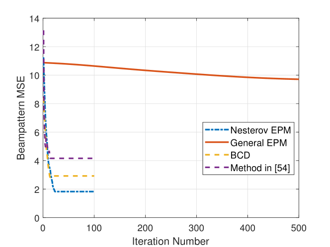
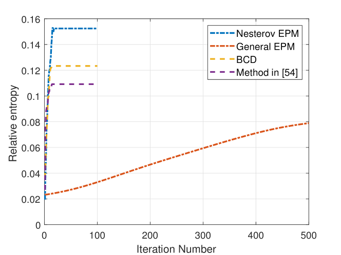
Figure 9: The convergence performance of the proposed one-bit beamforming method. (a) The beampattern MSE of the designed one-bit beamformers versus iteration number, (b) the relative entropy of the designed one-bit beamformers versus iteration number.

Fig. 10(a) shows the relative entropy values of one-bit beamformer versus the number of ADC bits for different numbers of transmit antennas. Apparently, as the number of the ADC bit increases, the relative entropy of one-bit beamformer becomes better and better, and when the ADC bit is large than 4, there is no significant improvement of the relative entropy by increasing the ADC bit. This clearly motivates us to adopt the low-resolution ADCs at the receiver, since it is favored by reducing the hardware cost and circuit power consumption. Besides, from the figure, we see that the system with one-bit phase shifters and one-bit ADCs benefits a lot from increasing the number of the transmit antennas, which suggests that we can increase the number of antennas to reduce the loss caused by one-bit phase shifters. Fig.10(b) and Fig.10(c) plot the probabilities of detection versus SNR value for different numbers of ADC bits and transmit antennas, respectively. The results agree with our expectations.

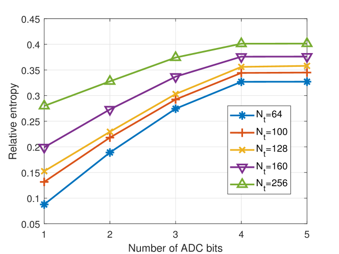
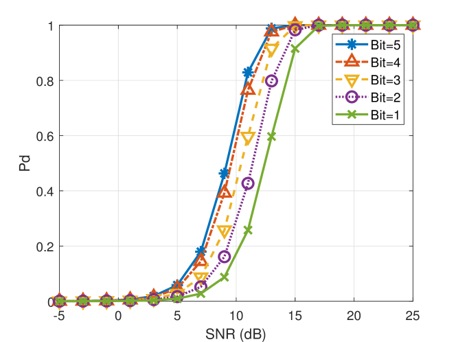
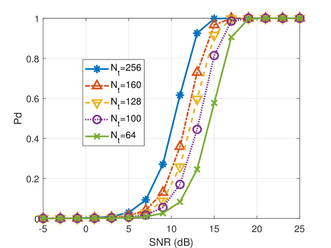
Figure 10: Performance of the designed one-bit beamformers. (a) The relative entropy values versus number of ADC bits for different numbers of transmit antennas, (b) The detection performance versus SNR for different quantization levels $\rm Bit$, $N_{t}=128$. $P_{\rm fa}=10^{-4}$. (c) The detection performance versus SNR for different numbers of transmit antennas when considering one-bit ADCs adopted at the receiver. $P_{\rm fa}=10^{-4}$

VI Conclusion

This paper has considered the problem of constant-envelope beamforming design for mmWave large-scale system with low-cost hardware architecture, in which the transmit array adopts a hybrid digital/analog beamforming and the receive array adopts low-resolution ADCs. The corresponding problem of constant-envelope beamforming is formulated via the relative entropy criterion. To deal with the nonconvex problem, we have developed a two-stage optimization framework based on the MM technique. We also have considered the constant-envelope beamforming with one-bit phase shifters, and developed an efficient iteration method based on the EPM and Nesterov-like method. The performance of the proposed schemes in terms of the relative entropy value and detection performance are assessed by numerical simulations. The simulation results show that the proposed beamforming is more efficient than the existing methods. More importantly, we also find that as the number of ADC bits increases, the improvement of the detection performance becomes more and more inapparent. Specifically, when the ADC bit number is larger than 3, the performance gap to the ideal ADCs is very small. In addition, when considering one-bit beamforming, we observe that the system benefits a lot from increasing the number of the transmit antennas.

Appendix A Proof of Lemma 1

Considering that the $K+1$ independent directions $\{\theta_{k}\}$ are randomly and uniformly distributed in $[-\pi/2,\pi/2]$, we have

$${\bf a}_{r}^{H}(\theta_{k}){\bf a}_{r}(\theta_{l})=\frac{1}{{{N_{r}}}}\sum\limits_{n=0}^{{N_{r}}-1}{{e^{j\pi n(\sin\theta_{k}-\sin\theta_{l})}}}$$ (43)

Then, we get

$${\mathbb{E}}\left({\bf a}_{r}^{H}(\theta_{k}){\bf a}_{r}(\theta_{l})\right)=\frac{1}{{{N_{r}}}}+\frac{1}{{{N_{r}}}}\sum\limits_{n=1}^{{N_{r}}-1}{\mathbb{E}}\left({{e^{j\pi n(\sin{\theta_{k}-\sin\theta_{l}})}}}\right)$$ (44)

$$\quad=\frac{1}{{{N_{r}}}}+\frac{1}{{{N_{r}}}}\sum\limits_{n=1}^{{N_{r}}-1}{\mathbb{E}}_{\theta_{l}}\left({{e^{-j\pi n\sin\theta_{l}}}}\right){\mathbb{E}}_{\theta_{k}}\left({{e^{j\pi n\sin\theta_{k}}}}\right)$$

Now, we calculate ${\mathbb{E}}_{\theta_{k}}\left({{e^{j\pi n\sin\theta_{k}}}}\right)$ as

$${\mathbb{E}}_{\theta_{k}}\left({{e^{j\pi n\sin\theta_{k}}}}\right) =\frac{1}{\pi}\int_{-\frac{\pi}{2}}^{\frac{\pi}{2}}{{e^{j\pi n\left({\sin{\theta_{k}}}\right)}}{\rm{d}}{\theta_{k}}}$$ (45)

$$=\frac{1}{\pi}\int_{-\frac{\pi}{2}}^{\frac{\pi}{2}}{\cos(\pi n\sin{\theta_{k}})+j\sin(\pi n\sin{\theta_{k}}){\rm{d}}{\theta_{k}}}$$

Due to the fact that $\cos(\pi n\sin{\theta_{k}})$ and $\sin(\pi n\sin{\theta_{k}})$ are even and odd functions with respect to $\theta_{k}$, respectively, we have

$${\mathbb{E}}_{\theta_{k}}\left({{e^{j\pi n\sin\theta_{k}}}}\right) =\frac{2}{\pi}\int_{0}^{\frac{\pi}{2}}{\cos(\pi n\sin{\theta_{k}}){\rm{d}}{\theta_{k}}}$$ (46)

$$=\frac{1}{\pi}\int_{0}^{\pi}{\cos(\pi n\sin{\theta_{k}}){\rm{d}}{\theta_{k}}}$$

$$=\frac{1}{2\pi}\int_{0}^{2\pi}{\cos(\pi n\sin{\theta_{k}}){\rm{d}}{\theta_{k}}}\buildrel\wedge\over{=}{J}_{0}(\pi n)$$

where ${J}_{0}(\pi n)$ is the Bessel function with the zero-th order [59]. Thus, we have

$${\mathbb{E}}\left({\bf a}_{r}^{H}(\theta_{k}){\bf a}_{r}(\theta_{l})\right)=\frac{1}{{{N_{r}}}}+\frac{1}{{{N_{r}}}}\sum\limits_{n=1}^{{N_{r}}-1}{J}_{0}^{2}(\pi n)$$ (47)

According to the property of ${J}_{0}(\pi n)$ that the series $\{{J}_{0}(\pi n)\}_{n=1}^{N_{r}-1}$ is attenuated, and ${J}_{0}(\pi n)\to\sqrt{\frac{2}{{\pi(\pi n)}}}\cos\left({\pi n-\frac{\pi}{4}}\right)={(-1)^{n}}\sqrt{\frac{1}{{{\pi^{2}}n}}}$ for large $n$ ([59], section 9.2.1). Then, we have that

$$\lim_{n\to\infty}\frac{\frac{1}{N_{r}}J_{0}^{2}(\pi n)}{\frac{1}{N_{r}\pi^{2}n}}=1$$ (48)

Since $J_{0}^{2}(\pi n)>0,\frac{1}{\pi^{2}n}>0$, there must exist a constant $\cal K$ such that when $n>\cal K$, we have

$$\frac{\frac{1}{N_{r}}J_{0}^{2}(\pi n)}{\frac{1}{N_{r}\pi^{2}n}}<2$$ (49)

Then, one gets

$$0 \leq\frac{1}{N_{r}}\sum_{n=1}^{N_{r}}J_{0}^{2}(\pi n)=\frac{1}{N_{r}}\sum_{n=1}^{\cal K}J_{0}^{2}(\pi n)+\frac{1}{N_{r}}\sum_{{{n=\mathcal{K}+1}}}^{N_{r}}J_{0}^{2}(\pi n)$$ (50)

$$\leq\frac{1}{N_{r}}\sum_{n=1}^{\cal K}J_{0}^{2}(\pi n)+\frac{2}{N_{r}}\sum_{n={\mathcal{K}}+1}^{N_{r}}\frac{1}{\pi^{2}n}$$

$$\leq\frac{1}{N_{r}}\sum_{n=1}^{\cal K}J_{0}^{2}(\pi n)+\frac{2}{N_{r}}\sum_{n=1}^{N_{r}}\frac{1}{\pi^{2}n}$$

Due to the fact that

$$0<\frac{1}{N_{r}\pi^{2}n}<\frac{1}{N_{r}^{(1-\epsilon)}\pi^{2}n^{(\epsilon+1)}}$$ (51)

and that

$$\mathop{\lim}\limits_{{N_{r}}\to\infty}\frac{1}{{N_{r}^{(1-\epsilon)}}}\sum\nolimits_{n=1}^{{N_{r}}}{\frac{1}{{{\pi^{2}}{n^{(\epsilon+1)}}}}}=0$$ (52)

where $0<\epsilon<1$, we can obtain that

$$\mathop{\lim}\limits_{{N_{r}}\to\infty}\frac{1}{{N_{r}}}\sum\nolimits_{n=1}^{{N_{r}}}{\frac{1}{{{\pi^{2}}{n}}}}=0$$ (53)

On the other hand, since $\sum_{n=1}^{\cal K}J_{0}^{2}(\pi n)$ is bounded, one can arrive at

$$\mathop{\lim}\limits_{{N_{r}}\to\infty}\frac{1}{{N_{r}}}\sum_{n=1}^{\cal K}J_{0}^{2}(\pi n)=0$$ (54)

Substituting (54) and (53) into (50), one gets that

$$0 \leq\mathop{\lim}\limits_{{N_{r}}\to\infty}\frac{1}{N_{r}}\sum_{n=1}^{N_{r}}J_{0}^{2}(\pi n)$$ (55)

$$\leq\mathop{\lim}\limits_{{N_{r}}\to\infty}\frac{1}{N_{r}}\sum_{n=1}^{\cal K}J_{0}^{2}(\pi n)+\frac{2}{N_{r}}\sum_{n=1}^{N_{r}}\frac{1}{\pi^{2}n}=0$$

Thus, $\mathop{\lim}\limits_{{N_{r}}\to\infty}\frac{1}{N_{r}}\sum_{n=1}^{N_{r}}J_{0}^{2}(\pi n)=0$, which implies that ${\mathbb{E}}\left({\bf a}_{r}^{H}(\theta_{k}){\bf a}_{r}(\theta_{l})\right)\to 0$ when $N_{r}\to\infty$.

Furthermore, we have ${\mathbb{V}}{\rm ar}\left({\bf a}_{r}^{H}(\theta_{k}){\bf a}_{r}(\theta_{l})\right)$ as

$${\mathbb{V}}{\rm ar}\left({\bf a}_{r}^{H}(\theta_{k}){\bf a}_{r}(\theta_{l})\right)={\mathbb{E}}\left({{{\left|{{\bf{a}}_{r}^{H}({\theta_{k}}){{\bf{a}}_{r}}({\theta_{l}})}\right|}^{2}}}\right)$$

$$=\frac{{{N_{r}}-1}}{{N_{r}^{2}}}+\frac{1}{{N_{r}^{2}}}\sum\limits_{m\neq n}^{{N_{r}}-1}{\sum\limits_{n=1}^{{N_{r}}-1}{\mathbb{E}}\left({{e^{j\pi(m-n)(\sin{\theta_{k}}-\sin{\theta_{l}})}}}\right)}+\frac{1}{{N_{r}^{2}}}$$

$$\qquad+\frac{2}{{N_{r}^{2}}}\Re\left\{{\sum\limits_{n=1}^{{N_{r}}-1}{\mathbb{E}}\left({{e^{j\pi n\left({\sin{\theta_{k}}-\sin{\theta_{l}}}\right)}}}\right)}\right\}$$

$$=\frac{1}{{N_{r}}}+\frac{1}{{N_{r}^{2}}}\sum\limits_{m\neq n}^{{N_{r}}-1}{\sum\limits_{n=1}^{{N_{r}}-1}{\mathbb{E}}\left({{e^{j\pi(m-n)(\sin{\theta_{k}}-\sin{\theta_{l}})}}}\right)}$$

$$=\frac{1}{{N_{r}}}+\frac{1}{{N_{r}^{2}}}\sum\limits_{m\neq n}^{{N_{r}}-1}{\sum\limits_{n=1}^{{N_{r}}-1}{J}_{0}^{2}(\pi(m-n))}$$

Further, we obtain that

$$\frac{1}{N_{r}^{2}}\sum_{m\neq n}^{N_{r}-1} \sum_{n=1}^{N_{r}-1}J_{0}^{2}(\pi(m-n))$$ (57)

$$\leqq\frac{1}{N_{r}^{2}}\sum_{m=1}^{N_{r}-1}\sum_{n=1}^{N_{r}-1}J_{0}^{2}(\pi(m-n))$$ (58)

$$\leqq\frac{1}{N_{r}^{2}}\sum_{k=(2-N_{r})}^{N_{r}-2}(N_{r}-1)J_{0}^{2}(\pi k)$$ (59)

$${\leqq\frac{1}{{{N_{r}}}}J_{0}^{2}(0)+\frac{2}{{N_{r}}}\sum\limits_{k=1}^{{N_{r}}-1}{J_{0}^{2}(\pi k)}}$$ (60)

$${=\frac{1}{{{N_{r}}}}+\frac{2}{{N_{r}}}\sum\limits_{k=1}^{{N_{r}}-1}{J_{0}^{2}(\pi k)}}$$ (61)

Thus, similar to Eq. (47), we can infer that ${\mathbb{V}}{\rm ar}\left({\bf a}_{r}^{H}(\theta_{k}){\bf a}_{r}(\theta_{l})\right)\to 0$ when $N_{r}\to\infty$.

Appendix B Proof of Lemma 2

Defining $\tilde{\bf X}={\bf X}{\bf X}^{H}$ and $\tilde{\bf x}={\rm vec}(\tilde{\bf X})$, we have

$$g({\bf X})=\tilde{\bf x}^{H}({{\bf{u}}{{\bf{u}}^{H}}\otimes{{\bf{u}}^{*}}{{\bf{u}}^{T}}})\tilde{\bf x}\buildrel\Delta\over{=}g(\tilde{\bf x})$$

Using Taylor’s theorem[60], the second-order inequality of $g(\tilde{\bf x})$ at the point $\tilde{\bf x}^{(m)}$ is given by

$$g(\tilde{\bf x}) \leq g(\tilde{\bf x}^{(m)})$$ (62)

$$~{}~{}~{}+\Re\big{(}{\tilde{\bf x}^{{(m)}H}}({{\bf{u}}{{\bf{u}}^{H}}\otimes{{\bf{u}}^{*}}{{\bf{u}}^{T}}})(\tilde{\bf x}-\tilde{\bf x}^{(m)})\big{)}$$

$$~{}~{}~{}+\frac{{\lambda_{\rm max}\left({{\bf{u}}{{\bf{u}}^{H}}\otimes{{\bf{u}}^{*}}{{\bf{u}}^{T}}}\right)}}{{\rm{2}}}\left\|\tilde{\bf x}-\tilde{\bf x}^{(m)}\right\|^{2}$$

$$=\frac{{\lambda_{\rm max}\left({{\bf{u}}{{\bf{u}}^{H}}\otimes{{\bf{u}}^{*}}{{\bf{u}}^{T}}}\right)}}{{\rm{2}}}\left\|\tilde{\bf X}-\tilde{\bf X}^{(m)}\right\|_{F}^{2}$$

$$~{}~{}~{}+({{\bf{u}}^{T}}{\tilde{\bf X}^{(m)}}{{\bf{u}}^{*}})^{*}\left({{\bf{u}}^{T}}\tilde{\bf X}{\bf{u}}^{*}\right)$$

Based on ${\bf T}^{H}{\bf T}={\bf I}_{\rm RF}$ and $\left|{{\bf{T}}}(i,j)\right|=\frac{1}{\sqrt{N_{t}}},\forall i,j$, one gets

$$\left\|\tilde{\bf x}-\tilde{\bf x}^{(m)}\right\|^{2}=\left\|\tilde{\bf x}\right\|^{2}+\left\|\tilde{\bf x}^{(m)}\right\|^{2}-2\Re\big{(}\tilde{\bf x}^{H}\tilde{\bf x}^{(m)}\big{)}$$ (63)

$$={\rm vec}^{H}({\bf X}{\bf X}^{H}){\rm vec}({\bf X}{\bf X}^{H})$$

$$~{}~{}~{}+{\rm vec}^{H}({\bf X}^{(m)}{\bf X}^{{(m)}H}){\rm vec}({\bf X}^{(m)}{\bf X}^{{(m)}H})$$

$$~{}~{}~{}-2\Re\big{(}{\rm vec}^{H}({\bf X}{\bf X}^{H}){\rm vec}({\bf X}^{(m)}{\bf X}^{{(m)}H})\big{)}$$

$$={\bf x}^{H}\big{(}{\bf X}^{T}{\bf X}^{*}\otimes{\bf I}_{N_{t}}\big{)}{\bf x}+{\bf x}^{{(m)}H}\big{(}{\bf X}^{{(m)}T}{\bf X}^{{(m)}*}\otimes{\bf I}_{N_{t}}\big{)}{\bf x}^{(m)}$$

$$~{}~{}~{}-2\Re\big{(}{\rm Tr}({\bf X}{\bf X}^{H}{\bf X}^{{(m)}}{\bf X}^{{(m)}H})\big{)}$$

$$=2N_{\rm RF}-2\Re\big{(}{\rm Tr}({\bf X}{\bf X}^{H}{\bf X}^{{(m)}}{\bf X}^{{(m)}H})\big{)}$$

where ${\bf x}={\rm vec}\left({\bf X}\right)$.

Substituting (63) into (62), and ignoring the constant terms unrelated to $\bf X$ yields

$$g({\bf X})\leq({{\bf{u}}^{T}}{{\bf X}^{(m)}{\bf X}^{{(m)}H}}{{\bf{u}}^{*}})\left({{\bf{u}}^{T}}{\bf X}{\bf X}^{H}{\bf{u}}^{*}\right)$$ (64)

$$\quad-{{{\color[rgb]{0,0,0}\lambda_{\rm max}}\left({{\bf{u}}{{\bf{u}}^{H}}\otimes{{\bf{u}}^{*}}{{\bf{u}}^{T}}}\right)}}\Re\big{(}{\rm Tr}({\bf X}{\bf X}^{H}{\bf X}^{(m)}{\bf X}^{{(m)}H})\big{)}$$

$$\quad+{\color[rgb]{0,0,0}N_{\rm RF}{{{\color[rgb]{0,0,0}\lambda_{\rm max}}\left({{\bf{u}}{{\bf{u}}^{H}}\otimes{{\bf{u}}^{*}}{{\bf{u}}^{T}}}\right)}}}$$

Thus, we complete this proof.

Appendix C Proof of Lemma 3

According to Lemma 2 and (33), the majorizing function $\widetilde{\mathcal{Z}}(\mathbf{t},\mathbf{t}^{(m)})$ of $\mathcal{Z}(\mathbf{t})$ at the point $\mathbf{t}^{(m)}$ is defined as

$$\widetilde{\mathcal{Z}}(\mathbf{t},\mathbf{t}^{(m)})=\Re(\mathbf{t}^{(m)H}\widetilde{\mathbf{Q}}^{(m)}\mathbf{t})+\text{const.}$$ (65)

where $\widetilde{\mathbf{Q}}^{(m)}={\bf I}_{N_{\rm RF}}\otimes{\bf Q}^{(m)}-{\lambda_{\rm max}}({\bf I}_{N_{\rm RF}}\otimes{\bf Q}^{(m)}){\bf I}$ and $\text{const}=\sum\limits_{\theta_{p}\in\Theta_{P}}{|\hat{\phi}(\theta_{p})|^{2}}+2\varsigma N_{\rm RF}+N_{\rm RF}\lambda_{\rm max}({\bf I}_{N_{\rm RF}}\otimes{\bf Q}^{(m)})$.

Based on the basis of MM [43, 44], the majorizing function $\widetilde{\mathcal{Z}}(\mathbf{t},\mathbf{t}^{(m)})$ of $\mathcal{Z}(\mathbf{t})$ satisfy the following two conditions:

$$\widetilde{\mathcal{Z}}(\mathbf{t},\mathbf{t}^{(m)})\geq\mathcal{Z}(\mathbf{t})$$ (66a)

$$\widetilde{\mathcal{Z}}(\mathbf{t}^{(m)},\mathbf{t}^{(m)})=\mathcal{Z}(\mathbf{t}^{(m)})$$ (66b)

Then, it is easy to show that with MM scheme, the objective value is monotonically decreasing at each iteration, i.e.,

$$\mathcal{Z}(\mathbf{t}^{(m+1)})\mathop{\leq}\limits^{\text{(a)}}\widetilde{\mathcal{Z}}(\mathbf{t}^{(m+1)},\mathbf{t}^{(m)})\mathop{\leq}\limits^{\text{(b)}}\widetilde{\mathcal{Z}}(\mathbf{t}^{(m)},\mathbf{t}^{(m)})\mathop{=}\limits^{\text{(c)}}\mathcal{Z}(\mathbf{t}^{(m)})$$ (67)

where (a) and (c) hold since the properties of the majorization function, namely (66a) and (66b) respectively. The inequality (b) hold since the solution to problem (35) is optimal.

Thus, we complete this proof.

Appendix D Proof of Proposition 1

According to the definition of $\Psi$ and Cauchy-Schwarz inequality, we have that

$$\frac{N}{M}={\bf x}^{T}{\bf y}\leq\|{\bf x}\|\|{\bf y}\|\leq\|{\bf x}\|\sqrt{\frac{N}{M}}$$ (68)

Thus, we have $\|{\bf x}\|\geq\sqrt{\frac{N}{M}}$. Combining the set $-\frac{1}{\sqrt{M}}\leq{\bf x}\leq\frac{1}{\sqrt{M}}$, one gets the following set

$$\|{\bf x}\|\geq\sqrt{\frac{N}{M}},~{}0\leq|{x_{n}}|\leq\frac{1}{\sqrt{M}},\forall n$$

Thus, we have $|{x_{n}}|=\frac{1}{\sqrt{M}}$, i.e., $\left\{{\bf x}\in\frac{1}{\sqrt{M}}\left\{-1,~{}1\right\}^{N}\right\}$.

Appendix E COMPUTATION of $\nabla_{\bf t}{\cal F}_{\rho}({\bf t})$

Let ${\cal F}_{\rho}({\bf t})=\psi_{1}({\bf t})+\varsigma\psi_{2}({\bf T})$ denote the objective value of problem (40), where $\psi_{1}({\bf t})=\sum_{\theta_{p}\in\Theta_{P}}{({\bf t}^{T}{\bf\Phi}_{p}{\bf t}-\hat{\phi}_{p})^{2}}+\rho(N_{\rm RF}-\sqrt{N_{\rm RF}}\|{\bf t}\|)$ and $\psi_{2}({\bf T})=\left\|{\bf T}^{T}{\bf T}-{\bf I}_{N_{\rm RF}}\right\|^{2}_{F}$. Then, we can obtain the derivation of $\psi_{1}({\bf t})$ with respect to $t_{(j-1)N_{t}+i},j=1,\cdots,N_{\rm RF};i=1,\cdots,N_{t}$ as

$$\frac{{\partial{\psi_{1}}({\bf{t}})}}{{\partial{t_{(j-1){N_{t}}+i}}}}=$$ (69)

$$~{}~{}\sum\limits_{\theta_{p}\in\Theta_{P}}{({{\bf{t}}^{T}}{{\bf{\Phi}}_{p}}{\bf{t}}-{{\hat{\phi}}_{p}}){{\bf{\Phi}}_{p,((j-1){N_{t}}+i):}}{\bf{t}}}-\frac{\rho\sqrt{N_{\rm RF}}}{\|{\bf t}\|}t_{(j-1){N_{t}}+i}$$

where ${{{\bf{\Phi}}_{p,((j-1){N_{t}}+i):}}}$ denotes the $(j-1){N_{t}}+i$-th row of the matrix ${\bf{\Phi}}_{p}$ and $t_{(j-1){N_{t}}+i}$ stands for the $(j-1){N_{t}}+i$-th entry of the vector ${\bf t}$.

To proceed, to compute the derivative of $\psi_{2}({\bf T})$ with respect to $t_{(j-1)N_{t}+i}$ (i.e., $T_{i,j}$), we need to extract the contribution of $T_{ij}$ to $\psi_{2}({\bf T})$. More exactly, let ${\overline{\bf{T}}}_{i,j}$ be the matrix $\bf{T}$ whose $(i,j)$-th entry is zeroed, and ${\bf E}_{i,j}$ be an $N_{t}\times N_{\rm RF}$-dimensional matrix whose $(i,j)$-th element is 1 and 0 otherwise, then we have

$$\psi_{2}(T_{ij}) =\left\|{{{\left({{T_{ij}}{{\bf{E}}_{i,j}}+{{\overline{\bf{T}}}_{i,j}}}\right)}^{T}}\left({{T_{ij}}{{\bf{E}}_{i,j}}+{{\overline{\bf{T}}}_{i,j}}}\right)-{{\bf{I}}_{{N_{{\rm{RF}}}}}}}\right\|_{F}^{2}$$ (70)

$$={T_{ij}^{4}}+2T_{ij}^{3}{\rm Tr}\Big{(}{\bf{E}}_{i,j}^{T}{\bf{E}}_{i,j}\big{(}{\bf{E}}_{i,j}^{T}{\overline{\bf{T}}}_{i,j}+{\overline{\bf{T}}}_{i,j}^{T}{\bf{E}}_{i,j}\big{)}\Big{)}$$

$$~{}~{}~{}+2T_{ij}^{2}{\rm Tr}\Big{(}{\bf{E}}_{i,j}^{T}{\bf{E}}_{i,j}\big{(}{\overline{\bf{T}}}_{i,j}^{T}{\overline{\bf{T}}}_{i,j}-{\bf I}_{N_{\rm RF}}\big{)}\Big{)}$$

$$~{}~{}~{}+T_{ij}^{2}{\rm Tr}\Big{(}\big{(}{\bf{E}}_{i,j}^{T}{\overline{\bf{T}}}_{i,j}+{\overline{\bf{T}}}_{i,j}^{T}{\bf{E}}_{i,j}\big{)}^{2}\Big{)}$$

$$~{}~{}~{}+2T_{ij}{\rm Tr}\Big{(}\big{(}{\bf{E}}_{i,j}^{T}{\overline{\bf{T}}}_{i,j}+{\overline{\bf{T}}}_{i,j}^{T}{\bf{E}}_{i,j}\big{)}\big{(}{\overline{\bf{T}}}_{i,j}^{T}{\overline{\bf{T}}}_{i,j}-{\bf I}_{N_{\rm RF}}\big{)}\Big{)}$$

$$={T_{ij}^{4}}+2T_{ij}^{2}\big{[}{\overline{\bf{T}}}_{i,j}^{T}{\overline{\bf{T}}}_{i,j}-{\bf I}_{N_{\rm RF}}\big{]}_{j,j}+2T_{ij}^{2}\big{[}{\overline{\bf{T}}}_{i,j}{\overline{\bf{T}}}_{i,j}^{T}\big{]}_{i,i}$$

$$~{}~{}~{}+4T_{ij}\big{[}\overline{\bf{T}}_{i,j}\big{(}{\overline{\bf{T}}}_{i,j}^{T}{\overline{\bf{T}}}_{i,j}-{\bf I}_{N_{\rm RF}}\big{)}\big{]}_{i,j}+{\rm const.}$$

where ${\rm const.}$ is a constant term unrelated to $T_{i,j}$. Thus, we attain

$$\frac{{\partial{\psi_{2}}(T_{i,j})}}{{\partial T_{i,j}}}$$ (71)

$$\quad~{}~{}=4T_{i,j}^{3}+4T_{i,j}\left(\big{[}{\overline{\bf{T}}}_{i,j}^{T}{\overline{\bf{T}}}_{i,j}-{\bf I}_{N_{\rm RF}}\big{]}_{j,j}+\big{[}{\overline{\bf{T}}}_{i,j}{\overline{\bf{T}}}_{i,j}^{T}\big{]}_{i,i}\right)$$

$$\qquad~{}~{}~{}+4\big{[}\overline{\bf{T}}_{i,j}\big{(}{\overline{\bf{T}}}_{i,j}^{T}{\overline{\bf{T}}}_{i,j}-{\bf I}_{N_{\rm RF}}\big{)}\big{]}_{i,j}$$

References

- [1] Y. Lin, T. Lee, Y. Pan, and K. Lin, “Low-complexity high-resolution parameter estimation for automotive MIMO radars,” IEEE Access, vol. 8, pp. 16 127–16 138, 2020.
- [2] P. Kumari, J. Choi, N. González-Prelcic, and R. W. Heath, “IEEE 802.11ad-based radar: an approach to joint vehicular communication-radar system,” IEEE Transactions on Vehicular Technology, vol. 67, no. 4, pp. 3012–3027, 2018.
- [3] S. H. Dokhanchi, B. S. Mysore, K. V. Mishra, and B. Ottersten, “A mmWave automotive joint radar-communications system,” IEEE Transactions on Aerospace and Electronic Systems, vol. 55, no. 3, pp. 1241–1260, 2019.
- [4] S. H. Dokhanchi, M. R. Bhavani Shankar, K. V. Mishra, T. Stifter, and B. Ottersten, “Performance analysis of mmWave bi-static PMCW-based automotive joint radar-communications system,” in 2019 IEEE Radar Conference (RadarConf), 2019, pp. 1–6.
- [5] W. L. Chan, J. R. Long, M. Spirito, and J. J. Pekarik, “A 60GHz-band 1v 11.5dbm power amplifier with 11% PAE in 65nm CMOS,” in 2009 IEEE International Solid-State Circuits Conference - Digest of Technical Papers, 2009, pp. 380–381,381a.
- [6] A. Valdes-Garcia, S. Reynolds, and J. Plouchart, “60 GHz transmitter circuits in 65nm CMOS,” in 2008 IEEE radio frequency integrated circuits symposium, 2008, pp. 641–644.
- [7] C. H. Doan, S. Emami, D. A. Sobel, A. M. Niknejad, and R. W. Brodersen, “Design considerations for 60 GHz CMOS radios,” IEEE Communications Magazine, vol. 42, no. 12, pp. 132–140, 2004.
- [8] E. Zhang and C. Huang, “On achieving optimal rate of digital precoder by RF-baseband codesign for MIMO systems,” in 2014 IEEE 80th Vehicular Technology Conference (VTC2014-Fall). IEEE, 2014, pp. 1–5.
- [9] O. E. Ayach, S. Rajagopal, S. Abu-Surra, Z. Pi, and R. W. Heath, “Spatially sparse precoding in millimeter wave MIMO systems,” IEEE Transactions on Wireless Communications, vol. 13, no. 3, pp. 1499–1513, 2014.
- [10] L. Liang, W. Xu, and X. Dong, “Low-complexity hybrid precoding in massive multiuser MIMO systems,” IEEE Wireless Communications Letters, vol. 3, no. 6, pp. 653–656, 2014.
- [11] L. Dai, X. Gao, J. Quan, S. Han, and I. Chih-Lin, “Near-optimal hybrid analog and digital precoding for downlink mmWave massive MIMO systems,” in 2015 IEEE International Conference on Communications (ICC). IEEE, 2015, pp. 1334–1339.
- [12] X. Yu, J.-C. Shen, J. Zhang, and K. B. Letaief, “Alternating minimization algorithms for hybrid precoding in millimeter wave MIMO systems,” IEEE Journal of Selected Topics in Signal Processing, vol. 10, no. 3, pp. 485–500, 2016.
- [13] S. Han, I. Chih-Lin, Z. Xu, and C. Rowell, “Large-scale antenna systems with hybrid analog and digital beamforming for millimeter wave 5G,” IEEE Communications Magazine, vol. 53, no. 1, pp. 186–194, 2015.
- [14] F. Sohrabi and W. Yu, “Hybrid digital and analog beamforming design for large-scale antenna arrays,” IEEE Journal of Selected Topics in Signal Processing, vol. 10, no. 3, pp. 501–513, 2016.
- [15] R. Rajamäki, S. P. Chepuri, and V. Koivunen, “Hybrid beamforming for active sensing using sparse arrays,” IEEE Transactions on Signal Processing, vol. 68, pp. 6402–6417, 2020.
- [16] Z. Xu, F. Liu, K. Diamantaras, C. Masouros, and A. Petropulu, “Learning to select for MIMO radar based on hybrid analog-digital beamforming,” in ICASSP 2021 - 2021 IEEE International Conference on Acoustics, Speech and Signal Processing (ICASSP), 2021, pp. 8228–8232.
- [17] Z. Cheng, L. Wu, B. Wang, M. R. Bhavani Shankar, and B. Ottersten, “Double-phase-shifter based hybrid beamforming for mmWave DFRC in the presence of extended target and clutters,” IEEE Transactions on Wireless Communications, pp. 1–1, 2022.
- [18] Z. Cheng, L. Wu, B. Wang, B. Shankar, B. Liao, and B. Ottersten, “Hybrid beamforming in mmWave dual-function radar-communication systems: Models, technologies, and challenges,” arXiv preprint arXiv:2209.04656, 2022.
- [19] Bin Le, T. W. Rondeau, J. H. Reed, and C. W. Bostian, “Analog-to-digital converters,” IEEE Signal Processing Magazine, vol. 22, no. 6, pp. 69–77, 2005.
- [20] J. Mo, P. Schniter, N. G. Prelcic, and R. W. Heath, “Channel estimation in millimeter wave MIMO systems with one-bit quantization,” in 2014 48th Asilomar Conference on Signals, Systems and Computers, 2014, pp. 957–961.
- [21] S. Wang, Y. Li, and J. Wang, “Multiuser detection in massive spatial modulation MIMO with low-resolution ADCs,” IEEE Transactions on Wireless Communications, vol. 14, no. 4, pp. 2156–2168, 2015.
- [22] O. Y. Kolawole, S. Biswas, K. Singh, and T. Ratnarajah, “Transceiver design for energy-efficiency maximization in mmWave MIMO IoT networks,” IEEE Transactions on Green Communications and Networking, vol. 4, no. 1, pp. 109–123, 2020.
- [23] J. Mo, P. Schniter, and R. W. Heath, “Channel estimation in broadband millimeter wave MIMO systems with few-bit ADCs,” IEEE Transactions on Signal Processing, vol. 66, no. 5, pp. 1141–1154, 2018.
- [24] C.-K. Wen, C.-J. Wang, S. Jin, K.-K. Wong, and P. Ting, “Bayes-optimal joint channel-and-data estimation for massive MIMO with low-precision ADCs,” IEEE Transactions on Signal Processing, vol. 64, no. 10, pp. 2541–2556, 2016.
- [25] A. K. Fletcher, S. Rangan, V. K. Goyal, and K. Ramchandran, “Robust predictive quantization: analysis and design via convex optimization,” IEEE Journal of Selected Topics in Signal Processing, vol. 1, no. 4, pp. 618–632, 2007.
- [26] M. Srinivasan and S. Kalyani, “Analysis of massive MIMO with low-resolution ADC in nakagami- fading,” IEEE Communications Letters, vol. 23, no. 4, pp. 764–767, 2019.
- [27] L. Fan, S. Jin, C. Wen, and H. Zhang, “Uplink achievable rate for massive MIMO systems with low-resolution ADC,” IEEE Communications Letters, vol. 19, no. 12, pp. 2186–2189, 2015.
- [28] K. Roth and J. A. Nossek, “Achievable rate and energy efficiency of hybrid and digital beamforming receivers with low resolution ADC,” IEEE Journal on Selected Areas in Communications, vol. 35, no. 9, pp. 2056–2068, 2017.
- [29] K. Roth, H. Pirzadeh, A. L. Swindlehurst, and J. A. Nossek, “A comparison of hybrid beamforming and digital beamforming with low-resolution ADCs for multiple users and imperfect CSI,” IEEE Journal of Selected Topics in Signal Processing, vol. 12, no. 3, pp. 484–498, 2018.
- [30] L. Zhao, M. Li, C. Liu, S. V. Hanly, I. B. Collings, and P. A. Whiting, “Energy efficient hybrid beamforming for multi-user millimeter wave communication with low-resolution A/D at transceivers,” IEEE Journal on Selected Areas in Communications, vol. 38, no. 9, pp. 2142–2155, 2020.
- [31] X. Huang, S. Bi, and B. Liao, “Direction-of-arrival estimation based on quantized matrix recovery,” IEEE Communications Letters, vol. 24, no. 2, pp. 349–353, 2020.
- [32] F. Xi, Y. Xiang, Z. Zhang, S. Chen, and A. Nehorai, “Joint angle and doppler frequency estimation for MIMO radar with one-bit sampling: a maximum likelihood-based method,” IEEE Transactions on Aerospace and Electronic Systems, vol. 56, no. 6, pp. 4734–4748, 2020.
- [33] S. Sedighi, B. S. Mysore R, M. Soltanalian, and B. Ottersten, “On the performance of one-bit DoA estimation via sparse linear arrays,” IEEE Transactions on Signal Processing, vol. 69, pp. 6165–6182, 2021.
- [34] M. Deng, Z. Cheng, L. Wu, B. Shankar, and Z. He, “One-bit ADCs/DACs based MIMO radar: Performance analysis and joint design,” IEEE Transactions on Signal Processing, vol. 70, pp. 2609–2624, 2022.
- [35] P. M. Woodward, Probability and information theory, with applications to radar: international series of monographs on electronics and instrumentation. Elsevier, 2014, vol. 3.
- [36] A. Leshem, O. Naparstek, and A. Nehorai, “Information theoretic adaptive radar waveform design for multiple extended targets,” IEEE Journal of Selected Topics in Signal Processing, vol. 1, no. 1, pp. 42–55, 2007.
- [37] Y. Yang and R. S. Blum, “Minimax robust MIMO radar waveform design,” IEEE Journal of Selected Topics in Signal Processing, vol. 1, no. 1, pp. 147–155, 2007.
- [38] B. Tang, J. Tang, and Y. Peng, “MIMO radar waveform design in colored noise based on information theory,” IEEE Transactions on Signal Processing, vol. 58, no. 9, pp. 4684–4697, 2010.
- [39] X. Song, P. Willett, S. Zhou, and P. B. Luh, “The MIMO radar and jammer games,” IEEE Transactions on Signal Processing, vol. 60, no. 2, pp. 687–699, 2012.
- [40] B. Tang, M. M. Naghsh, and J. Tang, “Relative entropy-based waveform design for MIMO radar detection in the presence of clutter and interference,” IEEE Transactions on Signal Processing, vol. 63, no. 14, pp. 3783–3796, 2015.
- [41] B. Tang, Y. Zhang, and J. Tang, “An efficient minorization maximization approach for MIMO radar waveform optimization via relative entropy,” IEEE Transactions on Signal Processing, vol. 66, no. 2, pp. 400–411, 2018.
- [42] M. M. Naghsh, M. Modarres-Hashemi, M. A. Kerahroodi, and E. H. M. Alian, “An information theoretic approach to robust constrained code design for mimo radars,” IEEE Transactions on Signal Processing, vol. 65, no. 14, pp. 3647–3661, 2017.
- [43] Y. Sun, P. Babu, and D. P. Palomar, “Majorization-minimization algorithms in signal processing, communications, and machine learning,” IEEE Transactions on Signal Processing, vol. 65, no. 3, pp. 794–816, 2017.
- [44] M. M. Naghsh, M. Modarres-Hashemi, S. ShahbazPanahi, M. Soltanalian, and P. Stoica, “Unified optimization framework for multi-static radar code design using information-theoretic criteria,” IEEE Transactions on Signal Processing, vol. 61, no. 21, pp. 5401–5416, 2013.
- [45] L. Wu, P. Babu, and D. P. Palomar, “Transmit waveform/receive filter design for MIMO radar with multiple waveform constraints,” IEEE Transactions on Signal Processing, vol. 66, no. 6, pp. 1526–1540, 2017.
- [46] H. A. Le Thi, H. M. Le, and T. P. Dinh, “Feature selection in machine learning: an exact penalty approach using a difference of convex function algorithm,” Machine Learning, vol. 101, no. 1-3, pp. 163–186, 2015.
- [47] G. Yuan and B. Ghanem, “Binary optimization via mathematical programming with equilibrium constraints,” arXiv preprint arXiv:1608.04425, 2016.
- [48] D. Jakovetić, J. M. F. Xavier, and J. M. F. Moura, “Convergence rates of distributed nesterov-like gradient methods on random networks,” IEEE Transactions on Signal Processing, vol. 62, no. 4, pp. 868–882, 2014.
- [49] A. K. Sahu, S. Kar, J. M. F. Moura, and H. V. Poor, “Distributed constrained recursive nonlinear least-squares estimation: algorithms and asymptotics,” IEEE Transactions on Signal and Information Processing over Networks, vol. 2, no. 4, pp. 426–441, 2016.
- [50] L. Xu, J. Li, and P. Stoica, “ Target detection and parameter estimation for MIMO radar systems,” IEEE Transactions on Aerospace and Electronic Systems, vol. 44, no. 3, pp. 927–939, 2008.
- [51] A. Hassanien and S. A. Vorobyov, “ Transmit energy focusing for DOA estimation in MIMO radar with colocated antennas,” IEEE Transactions on Signal Processing, vol. 59, no. 6, pp. 2669–2682, 2011.
- [52] A. Khabbazibasmenj, A. Hassanien, S. A. Vorobyov, and M. W. Morency, “Efficient transmit beamspace design for search-free based DOA estimation in MIMO radar,” IEEE Transactions on Signal Processing, vol. 62, no. 6, pp. 1490–1500, 2014.
- [53] T. M. Cover, Elements of information theory. John Wiley & Sons, 1999.
- [54] Z.-Q. Luo and P. Tseng, “On the convergence of the coordinate descent method for convex differentiable minimization,” Journal of Optimization Theory and Applications, vol. 72, no. 1, pp. 7–35, 1992.
- [55] R. V. Roland, “Simple and globally convergent methods for accelerating the convergence of any EM algorithm,” Scandinavian Journal of Stats, vol. 35, no. 2, pp. 335–353, 2010.
- [56] S. Boyd and L. Vandenberghe, Convex optimization. Cambridge university press, 2004.
- [57] Z. Cheng, Z. He, B. Liao, and M. Fang, “MIMO radar waveform design with PAPR and similarity constraints,” IEEE Transactions on Signal Processing, vol. 66, no. 4, pp. 968–981, 2018.
- [58] J.-C. Chen, “Alternating minimization algorithms for one-bit precoding in massive multiuser MIMO systems,” IEEE Transactions on Vehicular Technology, vol. 67, no. 8, pp. 7394–7406, 2018.
- [59] M. Abramowitz and I. A. Stegun, Handbook of mathematical functions with formulas, graphs, and mathematical tables. US Government printing office, 1964, vol. 55.
- [60] Y. Li and S. A. Vorobyov, “Fast algorithms for designing unimodular waveform(s) with good correlation properties,” IEEE Transactions on Signal Processing, vol. 66, no. 5, pp. 1197–1212, 2018.