Quantum Otto heat engines on XYZ spin working medium with DM and KSEA interactions: Operating modes and efficiency at maximal work output

Abstract

The magnetic Otto thermal machine based on a two-spin-1/2 XYZ working fluid in the presence of an inhomogeneous magnetic field and antisymmetric Dzyaloshinsky–Moriya (DM) and symmetric Kaplan–Shekhtman–Entin-Wohlman–Aharony (KSEA) interactions is considered. Its possible modes of operation are found and classified. The efficiencies of engines at maximum power are estimated for various choices of model parameters. There are cases when these efficiencies exceed the Novikov value. New additional points of local minima of the total work are revealed and the mechanism of their occurrence is analyzed.

1 Introduction

In 1955 Prokhorov and Basov BP55 ; BP55a ; BP55c , and later Bloembergen B56 proposed a three-level maser scheme with electromagnetic pump to obtain population inversion, which could lead to negative absorption. This scheme turned out to be very effective and was successfully implemented in masers SFS57 ; ZKMP58 ; ZKMP58a (and then in laser M60 ). Shortly after, Scovil and Schulz-DuBois came to a conclusion that “three-level masers can be regarded as heat engines”, and showed that “the limiting efficiency of a 3-level maser is that of a Carnot engine” SSDB59 (see also GSS67 ; GK94 ; GK96 ; LKAS17 ; GGKNLMSK18 ; S20 ). The induced (stimulated) emission in such a picture plays a role of the work output of heat engine, which operates between a hot pump temperature and a low relaxation bath temperature. So a three-level maser, as interpreted by Scovil and Schulz-DuBois, was the first example of a quantum heat engine and has become an important step in the development of quantum thermodynamics.

Quantum thermodynamics, which grew out of the classical Carnot theory C1824 , is based on the quantum-mechanical principles and deals with conditions of conservation and conversion of such forms of energy as heat and mechanical work VA16 ; BCGAA18 ; DC19 ; GMNK19 ; MAD22 (for a historical review see, e.g., AK18 ). Its important branch is the study of quantum cyclic heat engines that produce work using quantum matter as a working medium. There are many thermodynamic cycles QLSN07 ; Q09 . One of the most known among them is the Carnot cycle. It consists of isentropic compression and expansion and isothermal heat addition and rejection. All the processes that compose the ideal Carnot engine can be reversed, in which case it becomes a heat pump or refrigerator. The Carnot cycle provides an upper limit to the efficiency that any thermodynamic engine can achieve when converting heat to work, or vice versa.

Another important cycle is the Otto one. It is an idealized thermodynamic cycle that describes the operation of a spark-ignited piston engine in automobiles. The Otto cycle consists of four processes (strokes): two adiabatic ones, where there is no heat exchange and two isochoric ones, where there is no work exchange. Below, we will study magnetic quantum Otto cycles in which the “expansion” and “compression” of energy levels of the thermally isolated working fluid are performed during isochoric processes where work is the change in the average energy due to a change in external control parameters of the Hamiltonian of the system.

The magnetic Otto cycles and heat machines operating on spin quantum fluid have been studied by many researches (see Ref. PNCV20 and references therein). As a working substance one takes spin magnetic systems with Heisenberg pair and multi-spin non-local collective interactions. Much attention has been paid to cases when spin working medium involves Dzyaloshinsky-Moriya (DM) couplings Z08 ; ZZ17 ; AM21 . However, we are motivated to extend such studies and include in the consideration also Kaplan–Shekhtman–Entin-Wohlman–Aharony (KSEA) interactions Y20 ; FY21 , which are symmetric in contrast to the DM ones.

The structure of the paper is as follows. In Sect. 2, we briefly review quantum Otto cycles composed of two quantum adiabatic stages and two isochoric coupling to thermal baths (reservoirs). In Sect. 3, we describe the model of working medium used. Sect. 4 is devoted to the description of results obtained and their discussion. Finally, our main results are summarized in Sect 5.

2 Preliminaries

Before we start presenting our results, we should provide some necessary definitions and expressions used in this paper.

Let there be a system with Hamiltonian $H$, and its density operator $\rho$ satisfies, say, the quantum Liouville–von Neumann or Lindblad master equation, or has a thermal equilibrium Gibbs form. Here we will consider the latter case, that is

$$\rho=\frac{1}{Z}\exp(-\beta H),$$ (1)

where $Z={\rm Tr}\exp(-\beta H)$ is the partition function and $\beta=1/k_{B}T$, wherein $T$ is the temperature, and the Boltzmann constant $k_{B}$ is assumed to be equal to one for simplicity. The operator $\rho$ satisfies the following conditions: $\rho^{\dagger}=\rho$, $\rho\geq 0$, and ${\rm Tr}\rho=1$. Next, $F=-T\ln Z$ is the Helmholtz free energy and $S=-\partial F/\partial T$ denotes the entropy of the system.

The internal energy of the system is given as (see, e.g., DC19 )

$$U=\langle H\rangle=\sum_{n}p_{n}E_{n},$$ (2)

where $E_{n}$ are the energy levels and the density-matrix eigenvalues

$$p_{n}(T)=\frac{1}{Z(T)}\exp(-E_{n}/T)$$ (3)

represent the occupation probabilities of energy levels at the temperature $T$. From here, in accord with the first law of thermodynamics, it follows that during infinitesimal process the energy change equals K04

$$dU=\sum_{n}(E_{n}dp_{n}+p_{n}dE_{n})=\delta Q+\delta W,$$ (4)

where

$$\delta Q=\sum_{n}E_{n}dp_{n}$$ (5)

equals the heat transferred and

$$\delta W=\sum_{n}p_{n}dE_{n}$$ (6)

is the work done.

Note that positive heat, $Q>0$, means that heat is transferred to the working body, and its negative sign $Q<0$ means that heat, on the contrary, leaves the body. Similarly for the work. Positive amount of work, $\delta W>0$, corresponds to the work done on a given body by external forces, while negative work, $\delta W<0$, means that the body itself does work on some external object.

A cycle of the quantum Otto heat machine consists of four steps (see Fig. 1), namely, two adiabatic processes, where there is no heat exchange and two so-called isochoric (isomagnetic) ones, where there is no work exchange VA16 ; DC19 .

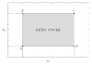
Figure 1: (Color online) Quantum Otto cycle in the $E_{n}-p_{n}$ plane. The cycle consists of two adiabatic ($AB$ and $CD$) and two isochoric ($BC$ and $DA$) processes

All processes are assumed to be sufficiently slow (quasistatic) and the quantum adiabatic theorem holds B27 ; BF28 ; M99 ; QZS05 ; LG18 ; IAL21 . According to this theorem, the level populations are invariant during the course of a quantum adiabatic process and, consequently, the von Neumann entropy remains unchanged. On the other hand, the classical adiabatic process is in equilibrium and characterized by a certain temperature at any given time, but not necessarily require that the occupation probabilities remain constant. The corresponding temperatures can be found, for example, from the Gibbs entropy invariance condition PNCV20 ; SB21 . Notice that the classical adiabatic theorem is a sequence of quantum adiabatic theorem, but the converse is not true in general.

Next, the cycle node with the lowest temperature $T_{c}$ can naturally be referred to the cold bath, and the node with the highest temperature $T_{h}$ to the hot one. Accordingly, the heat from or to the cold and hot baths will be denoted as $Q_{c}$ and $Q_{h}$, respectively.

Let us now consider in detail the Otto cycle shown in Fig. 1. It includes four following strokes.

First stroke ($AB$). The working medium at thermal equilibrium with the cold bath in $A$ at the temperature $T_{A}=T_{c}$ is isolated from thermal reservoir and undergoes an adiabatic compression (magnetization). Energy level parameters (spacings between energy levels) are increased, but the occupation probabilities stay unchanged. The work $W_{A\to B}=W_{in}$ is performed on the working medium during this step:

$$W_{A\to B}=\sum_{n}\int_{A}^{B}p_{n}dE_{n}=\sum_{n}p_{n}^{A}(E_{n}^{f}-E_{n}^{i}),$$ (7)

where $E_{n}^{i}$ and $E_{n}^{f}$ are the initial and final values of energy levels, respectively, and $p_{n}^{A}=p_{n}(T_{A})$ is the occupation probability by the temperature at the point $A$.

Second stroke ($BC$). The system is brought into thermal contact with the hot bath $C$ under unchanged its energy structure. This process is irreversible, and the occupation probabilities change to new equilibrium values. Only heat $Q_{B\to C}=Q_{h}$ is transformed in this step:

$$Q_{B\to C}=\sum_{n}\int_{B}^{C}E_{n}^{f}dp_{n}=\sum_{n}E_{n}^{f}(p_{n}^{C}-p_{n}^{B}),$$ (8)

where $p_{n}^{B}=p_{n}(T_{A})$ and $p_{n}^{C}=p_{n}(T_{C})$ are initial and final values of the occupation probabilities.

Third stroke ($CD$). This is another adiabatic (demagnetization) process reducing the energy gaps to initial values. Here, the external control parameters of system are changes back to the initial values and the occupation probabilities remain fixed. Only work $W_{C\to D}=W_{out}$ is performed by working medium and no heat is exchanged:

$$W_{C\to D}=\sum_{n}\int_{C}^{D}p_{n}dE_{n}=\sum_{n}p_{n}^{C}(E_{n}^{i}-E_{n}^{f}).$$ (9)

Fourth stroke ($DA$). The system is brought into thermal contact with the cold bath at node $A$. Again, no work is done, only heat $Q_{c}$ is rejected during this isochoric process:

$$Q_{D\to A}=\sum_{n}\int_{D}^{A}E_{n}^{i}dp_{n}=\sum_{n}E_{n}^{i}(p_{n}^{A}-p_{n}^{D}).$$ (10)

Since energy is conserved in a cyclic process, the balance condition is satisfied:

$$W_{A\to B}+Q_{B\to C}+W_{C\to D}+Q_{D\to A}=0$$ (11)

or

$$W+Q_{h}+Q_{c}=0,$$ (12)

where

$$W=W_{A\to B}+W_{C\to D}$$ (13)

is the total work. If $W<0$, the thermodynamical machine produces mechanical work $|W|=Q_{h}+Q_{c}$ with energy absorption $Q_{h}>0$ and energy release $Q_{c}<0$, i.e., corresponds to a heat engine; see Fig. 2.

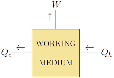
Figure 2: (Color online) Schematic layout of a heat engine. The arrows show the energy flows

The resulting work $W$ is performed during the exchange of heat $Q_{h}$ and $Q_{c}$ between the working fluid and the hot and cold baths.

Instead of drawing, we will further depict the engine as $\{\circ\!\leftarrow\uparrow\leftarrow\!\bullet\}$ (where the filled circle represents a hot bath and the open circle represents cold bath) or just like $\{\leftarrow\uparrow\leftarrow\}$ (left - cold bath, right- hot bath).

The efficiency of heat engine is defined as

$$\eta=\frac{|W|}{Q_{h}}.$$ (14)

In particular, the efficiency of an ideal Carnot cycle is given by the well-known expression

$$\eta_{C}=1-\frac{T_{c}}{T_{h}},$$ (15)

which is the upper bound for any thermodynamic cycles.

A heat engine acts by transferring energy from a warm region to a cool region of space and, in the process, converting some of that energy to mechanical work. The cycle may also be reversed. Then the system may be worked upon by an external force, and in the process, it can transfer thermal energy from a cooler system to a warmer one, thereby acting as a refrigerator or heat pump ($\{\rightarrow\downarrow\rightarrow\}$) rather than a heat engine. In this case, the operation of a heat machine is characterized by a coefficient of performance (CoP), which is defined as

$${\rm CoP}=\frac{Q_{c}}{W}.$$ (16)

This completes the preliminary section, and now we move on to the description of the working substance.

3 Working medium

As a working medium, we consider a two-site spin-1/2 system with the Hamiltonian

$$H = J_{x}\sigma_{1}^{x}\sigma_{2}^{x}+J_{y}\sigma_{1}^{y}\sigma_{2}^{y}+J_{z}\sigma_{1}^{z}\sigma_{2}^{z}+D_{z}(\sigma_{1}^{x}\sigma_{2}^{y}-\sigma_{1}^{y}\sigma_{2}^{x})+{\rm\Gamma}_{z}(\sigma_{1}^{x}\sigma_{2}^{y}+\sigma_{1}^{y}\sigma_{2}^{x})$$ (17)

$$+ B_{1}\sigma_{1}^{z}+B_{2}\sigma_{2}^{z},$$

where $\sigma_{i}^{\alpha}$ ($i=1,2$; $\alpha=x,y,z$) are the Pauli matrices, $B_{1}$ and $B_{2}$ the $z$-components of external magnetic fields applied at the first and second qubits respectively, ($J_{x}$,$J_{y}$,$J_{z}$) the vector of interaction constants of the Heisenberg part of interaction, $D_{z}$ the $z$-component of Dzyaloshinsky vector, and ${\rm\Gamma}_{z}$ the strength of KSEA interaction. Thus, this model contains seven real independent parameters: $B_{1}$, $B_{2}$, $J_{x}$, $J_{y}$, $J_{z}$, $D_{z}$, and ${\rm\Gamma}_{z}$.

In open matrix form, the Hamiltonian (17) reads

$$H=\left(\begin{array}[]{cccc}J_{z}+B_{1}+B_{2}&.&.&J_{x}-J_{y}-2i{\rm\Gamma}_{z}\\ .&-J_{z}+B_{1}-B_{2}&J_{x}+J_{y}+2iD_{z}&.\\ .&J_{x}+J_{y}-2iD_{z}&-J_{z}-B_{1}+B_{2}&.\\ J_{x}-J_{y}+2i{\rm\Gamma}_{z}&.&.&J_{z}-B_{1}-B_{2}\end{array}\right)$$ (18)

with the dots which are put instead of zero entries. This Hermitian matrix has X form. Its eigenvalues are equal to

$$E_{1,2}=J_{z}\pm R_{1},\qquad E_{3,4}=-J_{z}\pm R_{2},$$ (19)

where

$$R_{1}=[(B_{1}+B_{2})^{2}+(J_{x}-J_{y})^{2}+4{\rm\Gamma}_{z}^{2}]^{1/2},\quad R_{2}=[(B_{1}-B_{2})^{2}+(J_{x}+J_{y})^{2}+4D_{z}^{2}]^{1/2}.$$ (20)

Thus, the energy spectrum of the working medium consists of two pairs of levels with energy shifts $R_{1}$ and $R_{2}$. Therefore, instead of seven parameters, the spectrum is determined by only three quantities: $J_{z}$, $R_{1}$, and $R_{2}$. Note that ${\rm\Gamma}_{z}$ occurs only in $R_{1}$, while $D_{z}$ only in $R_{2}$, i.e., $R_{1}$ is the effective ${\rm\Gamma}_{z}$-parameter, and $R_{2}$, on the contrary, is the parameter determined by $D_{z}$.

The Gibbs density matrix is given by Eq. (1) and the partition function $Z=\sum_{n}\exp(-\beta E_{n})$ for the considered model is expressed as

$$Z=2[e^{-\beta J_{z}}\cosh(\beta R_{1})+e^{\beta J_{z}}\cosh(\beta R_{2})].$$ (21)

Therefore, the Gibbs entropy equals

$$S(T;J_{z},R_{1},R_{2})=-\frac{1}{Z}\biggl{[}\frac{R_{1}-J_{z}}{T}\exp\left(\frac{R_{1}-J_{z}}{T}\right)-\frac{R_{1}+J_{z}}{T}\exp\left(-\frac{R_{1}+J_{z}}{T}\right)$$

$$+\frac{R_{2}+J_{z}}{T}\exp\left(\frac{R_{2}+J_{z}}{T}\right)-\frac{R_{2}-J_{z}}{T}\exp\left(-\frac{R_{2}-J_{z}}{T}\right)\biggr{]}+\ln Z.$$ (22)

On the other hand, using Eq. (3), the von Neumann entropy

$$S=-\langle\ln\rho\rangle=-{\rm Tr}\rho\ln\rho=-\sum_{n}p_{n}\ln p_{n}$$ (23)

again leads to the Gibbs entropy expression (3).

Finally, using the general relations (7)–(10) and also (3) and (19), as well as taking into account the quantum adiabatic theorem, we arrive at equations for a heat engine with the considered working medium. For the adiabatic (isentropic) strokes, the equations are given as

$$W_{in}=$$

$$\Bigl{[}(J_{z}^{f}-J_{z}^{i})\Bigl{(}\cosh\frac{R_{1}^{i}}{T_{c}}e^{-J_{z}^{i}/T_{c}}-\cosh\frac{R_{2}^{i}}{T_{c}}e^{J_{z}^{i}/T_{c}}\Bigr{)}-(R_{1}^{f}-R_{1}^{i})\sinh\frac{R_{1}^{i}}{T_{c}}e^{-J_{z}^{i}/T_{c}}$$

$$-(R_{2}^{f}-R_{2}^{i})\sinh\frac{R_{2}^{i}}{T_{c}}e^{J_{z}^{i}/T_{c}}\Bigr{]}/\Bigl{(}\cosh\frac{R_{1}^{i}}{T_{c}}e^{-J_{z}^{i}/T_{c}}+\cosh\frac{R_{2}^{i}}{T_{c}}e^{J_{z}^{i}/T_{c}}\Bigr{)},$$ (24)

and

$$W_{out}=$$

$$\Bigl{[}(J_{z}^{i}-J_{z}^{f})\Bigl{(}\cosh\frac{R_{1}^{f}}{T_{h}}e^{-J_{z}^{f}/T_{h}}-\cosh\frac{R_{2}^{f}}{T_{h}}e^{J_{z}^{f}/T_{h}}\Bigr{)}-(R_{1}^{i}-R_{1}^{f})\sinh\frac{R_{1}^{f}}{T_{h}}e^{-J_{z}^{f}/T_{h}}$$

$$-(R_{2}^{i}-R_{2}^{f})\sinh\frac{R_{2}^{f}}{T_{h}}e^{J_{z}^{f}/T_{h}}\Bigr{]}/\Bigl{(}\cosh\frac{R_{1}^{f}}{T_{h}}e^{-J_{z}^{f}/T_{h}}+\cosh\frac{R_{2}^{f}}{T_{h}}e^{J_{z}^{f}/T_{h}}\Bigr{)}.$$ (25)

The net work done during a cycle is $W=W_{in}+W_{out}$.

Similarly for the isochoric strokes. The quantities of heat exchanged between working agent and hot and cold reservoirs, respectively, are

$$Q_{h}=\Bigl{[}\Bigl{(}J_{z}^{f}\cosh\frac{R_{1}^{f}}{T_{h}}-R_{1}^{f}\sinh\frac{R_{1}^{f}}{T_{h}}\Bigr{)}e^{-J_{z}^{f}/T_{h}}-\Bigl{(}J_{z}^{f}\cosh\frac{R_{2}^{f}}{T_{h}}$$

$$+R_{2}^{f}\sinh\frac{R_{2}^{f}}{T_{h}}\Bigr{)}e^{J_{z}^{f}/T_{h}}\Bigr{]}/\Bigl{(}\cosh\frac{R_{1}^{f}}{T_{h}}e^{-J_{z}^{f}/T_{h}}+\cosh\frac{R_{2}^{f}}{T_{h}}e^{J_{z}^{f}/T_{h}}\Bigr{)}$$

$$-\Bigl{[}\Bigl{(}J_{z}^{f}\cosh\frac{R_{1}^{i}}{T_{c}}-R_{1}^{f}\sinh\frac{R_{1}^{i}}{T_{c}}\Bigr{)}e^{-J_{z}^{i}/T_{c}}-\Bigl{(}J_{z}^{f}\cosh\frac{R_{2}^{i}}{T_{c}}$$

$$+R_{2}^{f}\sinh\frac{R_{2}^{i}}{T_{c}}\Bigr{)}e^{J_{z}^{i}/T_{c}}\Bigr{]}/\Bigl{(}\cosh\frac{R_{1}^{i}}{T_{c}}e^{-J_{z}^{i}/T_{c}}+\cosh\frac{R_{2}^{i}}{T_{c}}e^{J_{z}^{i}/T_{c}}\Bigr{)},$$ (26)

and

$$Q_{c}=\Bigl{[}\Bigl{(}J_{z}^{i}\cosh\frac{R_{1}^{i}}{T_{c}}-R_{1}^{i}\sinh\frac{R_{1}^{i}}{T_{c}}\Bigr{)}e^{-J_{z}^{i}/T_{c}}-\Bigl{(}J_{z}^{i}\cosh\frac{R_{2}^{i}}{T_{c}}$$

$$+R_{2}^{i}\sinh\frac{R_{2}^{i}}{T_{c}}\Bigr{)}e^{J_{z}^{i}/T_{c}}\Bigr{]}/\Bigl{(}\cosh\frac{R_{1}^{i}}{T_{c}}e^{-J_{z}^{i}/T_{c}}+\cosh\frac{R_{2}^{i}}{T_{c}}e^{J_{z}^{i}/T_{c}}\Bigr{)}$$

$$-\Bigl{[}\Bigl{(}J_{z}^{i}\cosh\frac{R_{1}^{f}}{T_{h}}-R_{1}^{i}\sinh\frac{R_{1}^{f}}{T_{h}}\Bigr{)}e^{-J_{z}^{f}/T_{h}}-\Bigl{(}J_{z}^{i}\cosh\frac{R_{2}^{f}}{T_{h}}$$

$$+R_{2}^{i}\sinh\frac{R_{2}^{f}}{T_{h}}\Bigr{)}e^{J_{z}^{f}/T_{h}}\Bigr{]}/\Bigl{(}\cosh\frac{R_{1}^{f}}{T_{h}}e^{-J_{z}^{f}/T_{h}}+\cosh\frac{R_{2}^{f}}{T_{h}}e^{J_{z}^{f}/T_{h}}\Bigr{)}.$$ (27)

The presented equations make it possible to investigate the quantum Otto heat engine in the general and various interesting special cases. Although, nonclassical correlations are initially present in the quantum state $\rho$ with Hamiltonian (17), transition to the diagonal energy representation, where the heat engine is analyzed, completely destroys any quantumness of correlations.

4 Results and discussion

Using the above equations, we will now study the operation of the quantum Otto machine in different modes.

4.1 A three-level system

Let us start with a simple case, namely, when $J_{z}=0$ and one of $R_{i}$ ($i=1,2$) is also equal to zero. Without loss of generality, we set $R_{2}=0$. In this case, the energy spectrum consists of three levels: doublet $E_{1,2}=\pm R_{1}$ and doubly-degenerate zero-energy level $E_{3,4}=0$.

It is important to note that here the energy levels are invariant under the scale transformation $E_{n}^{f}=qE_{n}^{i}$, where $q$ is independent of $n$. This property is necessary and sufficient condition that the quantum adiabatic theorem reduces to its classical counterpart LG18 . Thus, this is the case when the system is quantum but the adiabaticity condition is classical, i.e., quantum state at each point of the quantum adiabatic process is the state of thermal equilibrium with respect to the Hamiltonian at the given point.

On the other hand, the Gibbs entropy (3) for the case under discussion reduces to

$$S(T/R_{1})=2\Bigl{[}\ln 2+\ln\Bigl{(}\cosh\frac{R_{1}}{2T}\Bigr{)}-\frac{R_{1}}{2T}\tanh\frac{R_{1}}{2T}\Bigr{]},$$ (28)

i.e., it is a function of only one variable. Then the adiabaticity condition is $R_{1}/T=const$ and, therefore, adiabatic curves in the plane $R_{1}-T$ are straight lines passing through the origin of the coordinate system.

Otto cycles in the plane $R_{1}-temperature$ are shown in Fig. 3.

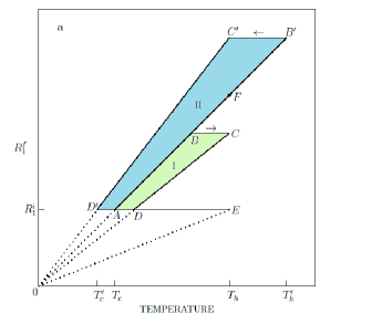
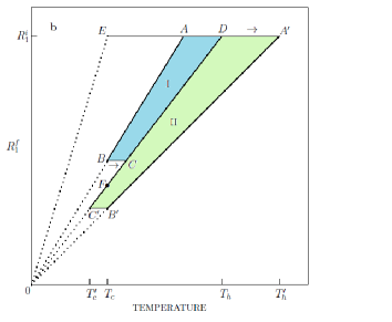
Figure 3: (Color online) Otto cycles of thermal machine in the case $J_{z}=R_{2}=0$ for $R_{1}^{f}\geq R_{1}^{i}$ (a) and $R_{1}^{f}\leq R_{1}^{i}$ (b). The green trapezoids correspond to engine cycles, and the blue ones represent refrigerator cycles. Other details are described in the text

If the final value of $R_{1}$ is equal to the initial value, $R_{1}^{f}=R_{1}^{i}$, then the cycle contracts into a segment of a horizontal straight line from temperature $T_{c}$ to $T_{h}$ ($AE$ in Fig. 3a and $ED$ in Fig. 3b).

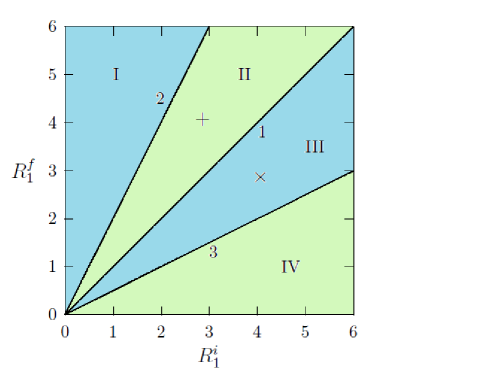
Figure 4: (Color online) Regions of different operating modes (regimes) in the plane ($R_{1}^{i},R_{1}^{f}$) for the quantum Otto thermal machine with nonzero $R_{1}$ and $J_{z}=R_{2}=0$ by $T_{c}=1$ and $T_{h}=2$. Here, 1 is the diagonal straight line $R_{1}^{f}=R_{1}^{i}$, 2 and 3 are the boundaries $R_{1}^{f}=(T_{h}/T_{c})R_{1}^{i}$ and $R_{1}^{f}=(T_{c}/T_{h})R_{1}^{i}$, respectively. Regions I and III (blue) correspond to the refrigeration regime, while the regions II and IV (green) represent the heat engine. The ‘+’ symbol has coordinates (2.86075,4.06548) and marks the position of minimum of $W$ ($=-0.148615$), and the ‘$\times$’ symbol has mirror coordinates (4.06548,2.86075) which mark the position of maximum of $W$ ($=0.148615$) in the region III

When $R_{1}^{f}$ starts to increase, the cycle ABCD appears that goes clockwise and has adiabatic $AB$ and $CD$ and isochoric $BC$ and $DA$ strokes (green trapezoid I in Fig. 3a). The nodes $A$ and $C$ correspond here to the cold and hot reservoirs: $T_{A}=T_{c}$ and $T_{C}=T_{h}$. The adiabaticity conditions allow us to express the temperatures of other two nodes through the temperatures of the cold and hot reservoirs: $T_{B}=T_{c}R_{1}^{f}/R_{1}^{i}$ and $T_{D}=T_{h}R_{1}^{i}/R_{1}^{f}$. Because of this, the net work performed during the whole cycle is given as

$$W=(R_{1}^{f}-R_{1}^{i})\Bigl{(}\tanh\frac{R_{1}^{f}}{2T_{h}}-\tanh\frac{R_{1}^{i}}{2T_{c}}\Bigr{)}.$$ (29)

This work equals zero, if $R_{1}^{f}=R_{1}^{i}$ or $R_{1}^{f}=(T_{h}/T_{c})R_{1}^{i}$.

On the other hand, $Q_{h}$ and $Q_{c}$ are given as

$$Q_{h}=R_{1}^{f}\Bigl{(}\tanh\frac{R_{1}^{i}}{2T_{c}}-\tanh\frac{R_{1}^{f}}{2T_{h}}\Bigr{)}.$$ (30)

and

$$Q_{c}=R_{1}^{i}\Bigl{(}\tanh\frac{R_{1}^{f}}{2T_{h}}-\tanh\frac{R_{1}^{i}}{2T_{c}}\Bigr{)}.$$ (31)

Both $Q_{h}$ and $Q_{c}$ equal zero at the same boundary $R_{1}^{f}=(T_{h}/T_{c})R_{1}^{i}$ as $W$. Below this line, $Q_{h}>0$ and $Q_{c}<0$. As a result, the region $0<R_{1}^{f}<(T_{h}/T_{c})R_{1}^{i}$ corresponds to the heat engine regime; see green domain II in Fig. 4. The structure of isolines of net work $W$ in this domain is depicted in Fig. 5.

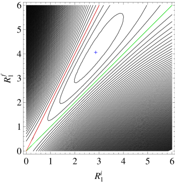
Figure 5: (Color online) Qualitative structure of isolines for the total work $W(R_{1}^{i},R_{1}^{f})$; here $J_{z}=R_{2}=0$, and bath temperatures $T_{c}=1$ and $T_{h}=2$. The region between the red ($R_{1}^{f}=2R_{1}^{i}$) and green ($R_{1}^{f}=R_{1}^{i}$) lines corresponds to the engine mode. The symbol “$+$” indicates the position of local minimum of the function $W(R_{1}^{i},R_{1}^{f})$

Taking into account the definition (14) and Eqs. (29)–(30), we get the efficiency of the given Otto heat engine

$$\eta=1-\frac{R_{1}^{i}}{R_{1}^{f}}.$$ (32)

Since $R_{1}^{f}<(T_{h}/T_{c})R_{1}^{i}$, the value found is less than Carnot’s efficiency (15). This agrees with the Carnot theorem (principle) known from classical thermodynamics. According to this theorem, no heat engine operating on a cycle between two heat reservoirs can be more efficient than a reversible heat engine operating between the same two reservoirs regardless of the working substance employed or the operation details; Carnot’s efficiency (15) is the upper limit that does not depend on the design of the engine (see, e.g., FLS64 , Chapt. 44).

The efficiency (32) is zero at $R_{1}^{f}=R_{1}^{i}$. When $R_{1}^{f}$ reaches the value of $(T_{h}/T_{c})R_{1}^{i}$, the Otto cycle is reduced to a section of straight line between points $A$ and $F$, as shown in Fig. 3a. The efficiency of such a “cycle” reaches a Carnot efficiency of $50\%$, however, the total work $W$, Eq. (29), vanishes here.

Further, if $R_{1}^{f}>(T_{h}/T_{c})R_{1}^{i}$, the cycle transforms into a trapezoid $AB^{\prime}C^{\prime}D^{\prime}$ shown in Fig. 3a by a blue region II. Note first of all, that the direction of such a cycle was changed to opposite. Moreover, the minimum temperature now is at the node $D^{\prime}$ and equals $T_{c}^{\prime}=(R_{1}^{i}/R_{1}^{f})T_{h}$, while the maximum one is at node $B^{\prime}$ and equals $T_{h}^{\prime}=(R_{1}^{f}/R_{1}^{i})T_{c}$. It is clear that $T_{c}^{\prime}<T_{c}$, $T_{h}^{\prime}>T_{h}$ and $T_{h}^{\prime}/T_{c}^{\prime}>T_{h}/T_{c}$. Hence, the total work

$$W=(R_{1}^{f}-R_{1}^{i})\Bigl{(}\tanh\frac{R_{1}^{f}}{2T_{h}}-\tanh\frac{R_{1}^{i}}{2T_{c}}\Bigr{)}=(R_{1}^{f}-R_{1}^{i})\Bigl{(}\tanh\frac{R_{1}^{i}}{2T_{c}^{\prime}}-\tanh\frac{R_{1}^{f}}{2T_{h}^{\prime}}\Bigr{)}>0.$$ (33)

The values of heat of cold and hot strokes are given as

$$Q_{c}\equiv Q_{D^{\prime}\to A}=R_{1}^{i}\Bigl{(}\tanh\frac{R_{1}^{f}}{2T_{h}}-\tanh\frac{R_{1}^{i}}{2T_{c}}\Bigr{)}=R_{1}^{i}\Bigl{(}\tanh\frac{R_{1}^{i}}{2T_{c}^{\prime}}-\tanh\frac{R_{1}^{f}}{2T_{h}^{\prime}}\Bigr{)}>0$$ (34)

and

$$Q_{h}\equiv Q_{B^{\prime}\to C^{\prime}}=R_{1}^{f}\Bigl{(}\tanh\frac{R_{1}^{i}}{2T_{c}}-\tanh\frac{R_{1}^{f}}{2T_{h}}\Bigr{)}=R_{1}^{f}\Bigl{(}\tanh\frac{R_{1}^{f}}{2T_{h}^{\prime}}-\tanh\frac{R_{1}^{i}}{2T_{c}^{\prime}}\Bigr{)}<0.$$ (35)

This regime corresponds to the refrigerator mode (blue region I in Fig. 4).

We discuss now the cases when $R_{1}^{f}$ is less than $R_{1}^{i}$. If $(T_{c}/T_{h})R_{1}^{i}<R_{1}^{f}<R_{1}^{i}$, typical cycle can be represented by a trapezoid $ABCD$ shown in Fig. 3b as blue region I. The cycle runs counterclockwise and cold and hot nodes are $B$ and $D$, respectively. The total work and heat are given by expressions

$$W=(R_{1}^{i}-R_{1}^{f})\Bigl{(}\tanh\frac{R_{1}^{f}}{2T_{c}}-\tanh\frac{R_{1}^{i}}{2T_{h}}\Bigr{)}>0,$$ (36)

$$Q_{c}=R_{1}^{f}\Bigl{(}\tanh\frac{R_{1}^{f}}{2T_{c}}-\tanh\frac{R_{1}^{i}}{2T_{h}}\Bigr{)}>0$$ (37)

and

$$Q_{h}=R_{1}^{i}\Bigl{(}\tanh\frac{R_{1}^{i}}{2T_{h}}-\tanh\frac{R_{1}^{f}}{2T_{c}}\Bigr{)}<0.$$ (38)

This is again the cooling mode of Otto’s thermal machine: $\{\rightarrow\downarrow\rightarrow\}$. For example, the coefficient of performance at the point of maximum total work in this case (see Fig. 4, the point marked with the symbol “$\times$”) reaches the value ${\rm CoP}=2.37$.

When $R_{1}^{f}=(T_{c}/T_{h})R_{1}^{i}$, the “cycle” is a straight-line section $DF$. Here, $W=Q_{c}=Q_{h}=0$.

Finally, if $R_{1}^{f}<(T_{c}/T_{h})R_{1}^{i}$ then the cycle is $DA^{\prime}B^{\prime}C^{\prime}$ shown as the green trapezoid II in Fig. 3b. In this case $W<0$, $Q_{c}<0$ and $Q_{h}>0$ and therefore the heat engine regime is realized here. In Fig. 4, the corresponding area is labeled IV and shown in green.

As mentioned above, the efficiency of the discussed Otto engine can reach the upper limit, namely, the Carnot efficiency. However, in this case, the total work performed is zero and therefore such an “engine” is useless. It is of interest to find the efficiency of engines at their maximum power (work per cycle).

In 1957, Novikov N57 considered a generalized Carnot engine taking into account the heat loss from the hot bath to the working fluid ($\{\leftarrow\uparrow\leftarrow\triangleleft\}$, where the triangle $\triangleleft$ denotes a lossy heat conductor) and derived a remarkable formula for the efficiency at maximum power of such an engine (Eq. (7) in Ref. N57 and Eq. (6) in Ref. N58 )

$$\eta_{N}=1-\sqrt{T_{c}/T_{h}}.$$ (39)

(In connection with the problem of optimal efficiency of engines, see Ref. VN72 .) More later, in 18 years, Curzon and Ahlborn CA75 ; AC04 (see also VLF14 ; F17 ) considered a Carnot engine with losses both from the hot bath to the working fluid and from the working fluid to the cold bath, $\{\triangleleft\leftarrow\uparrow\leftarrow\triangleleft\}$, and obtained the same result for the efficiency. This gave an impetus to the development of endoreversible thermodynamics DC19 ; H08 .

It turned out that efficiency (39) is the benchmark for the efficiency $\eta_{mp}$ of any real running engine at maximum power. Therefore, it is interesting to compare the efficiency at maximal power of the Otto engine with the Novikov efficiency. The efficiency for the engine operating between bath temperatures $T_{c}=1$ and $T_{h}=2$ at the point with the maximum work done ($|W|=0.148615$, see Figs. 4 and 5) equals $29.6\%$. This is less than Carnot’s efficiency of $50\%$, but larger than Novikov’s efficiency equaled $29.3\%$. A similar picture is also valid for other temperatures presented in Table 1.

Table 1: Coordinates ($R_{1}^{i}$ and $R_{1}^{f}$) of a minimum of the work $W$, its value at the minimum, efficiency at maximum power, and Carnot and Novikov efficiencies by $Tc=1$ and different values of $T_{h}$

$T_{h}$	$R_{1}^{i}$	$R_{1}^{f}$	$W$	$\eta_{mp}$	$\eta_{C}$	$\eta_{N}$
3	3.16836	5.59152	-0.454983	43.3%	66.7%	42.3%
2.5	3.02699	4.83933	-0.289598	37.5%	60%	36.8%
2	2.86075	4.06548	-0.148615	29.6%	50%	29.3%
1.5	2.65857	3.25929	-0.044155	18.43%	33.3%	18.35%

As seen from Table 1, both the useful work and efficiency grow with increasing the temperature difference of reservoirs. Note that these $\eta_{mp}$ values are well reproduced by Novikov’s formula, and moreover, they are somewhat greater than it provides. A similar increase in efficiency at maximum power has recently been obtained for a photonic engine SPD20 .

Thus, the Otto thermal machine on a spin working substance with $J_{z}=0$ and one of the two $R_{1}$ and $R_{2}$ equal to zero can operate either as an engine or as a refrigerator. The efficiency at maximum output power is limited from above by the Carnot bound, and from below by the Novikov efficiency.

4.2 Two local minima of net work done

In this section, we extend the case described above and consider the parameter $R_{2}$ as constant, not equal to zero. So $J_{z}=0$, $R_{2}=const$, and $R_{1}\in[R_{1}^{i},R_{1}^{f}]$.

From Eqs. (3) and (3), it follows that the net work done during a cycle is given as

$$W=(R_{1}^{f}-R_{1}^{i})\Bigl{[}\sinh\frac{R_{1}^{f}}{T_{h}}/\Bigl{(}\cosh\frac{R_{1}^{f}}{T_{h}}+\cosh\frac{R_{2}}{T_{h}}\Bigr{)}-\sinh\frac{R_{1}^{i}}{T_{c}}/\Bigl{(}\cosh\frac{R_{1}^{i}}{T_{c}}+\cosh\frac{R_{2}}{T_{c}}\Bigr{)}\Bigr{]}.$$ (40)

Next, in accordance with Eqs. (3) and (3), the heat $Q_{h}$ is

$$Q_{h}=\frac{R_{1}^{f}\sinh(R_{1}^{i}/T_{c})+R_{2}\sinh(R_{2}/T_{c})}{\cosh(R_{1}^{i}/T_{c})+\cosh(R_{2}/T_{c})}-\frac{R_{1}^{f}\sinh(R_{1}^{f}/T_{h})+R_{2}\sinh(R_{2}/T_{h})}{\cosh(R_{1}^{f}/T_{h})+\cosh(R_{2}/T_{h})}$$ (41)

and similarly for $Q_{c}$:

$$Q_{c}=\frac{R_{1}^{i}\sinh(R_{1}^{f}/T_{h})+R_{2}\sinh(R_{2}/T_{h})}{\cosh(R_{1}^{f}/T_{h})+\cosh(R_{2}/T_{h})}-\frac{R_{1}^{i}\sinh(R_{1}^{i}/T_{c})+R_{2}\sinh(R_{2}/T_{c})}{\cosh(R_{1}^{i}/T_{c})+\cosh(R_{2}/T_{c})}.$$ (42)

The boundaries separating the regions with $W>0$ and $W<0$ are found from condition $W=0$. It is obvious from (40), that one boundary is again the diagonal

$$R_{1}^{f}=R_{1}^{i},$$ (43)

while the other boundary is determined by the relation

$$R_{1}^{f}=T_{h}\ln\Biggl{[}\frac{1}{1-\gamma}\Biggl{(}\gamma\cosh\frac{R_{2}}{T_{h}}+\sqrt{1+\gamma^{2}\sinh^{2}\frac{R_{2}}{T_{h}}}\Biggr{)}\Biggr{]},$$ (44)

where

$$\gamma=\sinh\frac{R_{1}^{i}}{T_{c}}/\Bigl{(}\cosh\frac{R_{1}^{i}}{T_{c}}+\cosh\frac{R_{2}}{T_{c}}\Bigr{)}.$$ (45)

It is clear that $R_{1}^{f}=0$ at $R_{1}^{i}=0$. For small $R_{1}^{i}$, the dependence (44) behaves like

$$R_{1}^{f}\approx\kappa R_{1}^{i},$$ (46)

where

$$\kappa=\frac{T_{h}}{T_{c}}\Bigl{(}\frac{\cosh[R_{2}/(2T_{h})]}{\cosh[R_{2}/(2T_{c})]}\Bigr{)}^{2}.$$ (47)

For $\kappa=1$, these two boundaries touch near small $R_{1}^{i}$. On the other hand, when $R_{1}^{i}\to\infty$, the function $R_{1}^{f}$ of $R_{1}^{i}$, Eq. (44), satisfies the linear asymptotic law

$$R_{1}^{f}\approx T_{h}\ln\Bigl{(}\frac{\cosh(R_{2}/T_{h})}{\cosh(R_{2}/T_{c})}\Bigr{)}+\frac{T_{h}}{T_{c}}R_{1}^{i}.$$ (48)

Thus, for large $R_{1}^{i}$, the values of $R_{1}^{f}$ again follow, as in the previous subsection, a linear dependence $R_{1}^{f}=(T_{h}/T_{c})R_{1}^{i}$, but now shifted.

For bath temperatures $T_{c}=1$ and $T_{h}=2$, the slope coefficient (47) reaches the critical value $\kappa_{c}=1$ at $R_{2}^{(c)}=4\ln\big{[}\frac{1}{2}\big{(}\frac{1+\sqrt{5}}{\sqrt{2}}+\sqrt{\sqrt{5}-1}\big{)}\big{]}\simeq 2.12255$. When $R_{2}<R_{2}^{(c)}$, the engine mode has only one local minimum of the work $W$ (see Fig. 6a).

Figure 6: Regions with $W<0$ (between lines 1 and 2) and with $W>0$ (outside the previous region) in the plane $(R_{1}^{i},R_{1}^{f})$. Bath temperatures are $T_{c}=1$ and $T_{h}=2$. Dotted line $R_{1}^{f}=(T_{h}/T_{c})R_{1}^{i}$ is shown for a comparison with the case $R_{2}=0$. (a), $R_{2}=1.8$, the black circle ($\bullet$) has coordinates $(4.32922,5.51837)$ and indicates the local minimum of work ($W=-0.09977$). (b), $R_{2}=2.9$, black circle ($\bullet$) has coordinates $(5.62759,6.82585)$ and shows the minimum $W=-0.08299$, while the symbol plus (+) marks additional local minimum ($W=-0.00366$) at the point $(1.31298,1.15942)$

Here, both $R_{1}^{i}$ and $R_{1}^{f}$ are greater than $R_{2}$, and therefore there is no energy level crossing.

However, for $R_{2}>R_{2}^{(c)}$, the curve 2 forms a loop, inside which the second minimum appears (see Fig. 6b). In it, $R_{1}^{i}$ and $R_{1}^{f}$ are less than $R_{2}$, which means that again there is no energy level crossing. Engine efficiencies, defined by Eq. (14), in two minima shown in Fig. 6b are $\eta_{\bullet}=26.3\%$ and $\eta_{+}=0.58\%$. Both of these values are less than Novikov’s efficiency of $29.3\%$.

So, the presence of two minimums of optimal engine operating modes at once is a rather interesting situation, but it is not yet clear where and how it can be used in practice.

4.3 Three-parameter energy spectrum

We now turn to the quantum Otto machine, the working body of which is described by the Hamiltonian (17) with all interactions. The energy levels are characterized by three parameters $J_{z}$, $R_{1}$, and $R_{2}$.

Let the longitudinal exchange coupling $J_{z}$ vary within $J_{z}^{i}$ and $J_{z}^{f}$, while the parameters $R_{1}$ and $R_{2}$ remain unchanged during a cycle, that is $R_{1}^{i}=R_{1}^{f}=R_{1}$ and $R_{2}^{i}=R_{2}^{f}=R_{2}$. Equations (3) and (3) for the net work done take the form

$$W=(J_{z}^{f}-J_{z}^{i})$$

$$\times\Bigl{[}\Bigl{(}\cosh\frac{R_{1}}{T_{c}}e^{-J_{z}^{i}/T_{c}}-\cosh\frac{R_{2}}{T_{c}}e^{J_{z}^{i}/T_{c}}\Bigr{)}/\Bigl{(}\cosh\frac{R_{1}}{T_{c}}e^{-J_{z}^{i}/T_{c}}+\cosh\frac{R_{2}}{T_{c}}e^{J_{z}^{i}/T_{c}}\Bigr{)}$$

$$-\Bigl{(}\cosh\frac{R_{1}}{T_{h}}e^{-J_{z}^{f}/T_{h}}-\cosh\frac{R_{2}}{T_{h}}e^{J_{z}^{f}/T_{h}}\Bigr{)}/\Bigl{(}\cosh\frac{R_{1}}{T_{h}}e^{-J_{z}^{f}/T_{h}}+\cosh\frac{R_{2}}{T_{h}}e^{J_{z}^{f}/T_{h}}\Bigr{)}\Bigr{]}.$$

The boundaries separating the regions with $W>0$ and $W<0$ are given here like

$$J_{z}^{f}=J_{z}^{i}$$ (50)

and

$$J_{z}^{f}=\frac{T_{h}}{T_{c}}J_{z}^{i}+\frac{1}{2}T_{h}\ln\Biggl{(}\frac{\cosh(R_{1}/T_{h})\cosh(R_{2}/T_{c})}{\cosh(R_{1}/T_{c})\cosh(R_{2}/T_{h})}\Biggr{)}.$$ (51)

These straight lines intersect at a point defined by the presented equations.

Taken into account Eq. (3), the heat $Q_{h}$ for the case under consideration is reduced to

$$Q_{h}=A_{1}-\Bigl{[}\Bigl{(}J_{z}^{f}\cosh\frac{R_{1}}{T_{c}}-R_{1}\sinh\frac{R_{1}}{T_{c}}\Bigr{)}e^{-J_{z}^{f}/T_{c}}-\Bigl{(}J_{z}^{f}\cosh\frac{R_{2}}{T_{c}}$$

$$+R_{2}\sinh\frac{R_{2}}{T_{c}}\Bigr{)}e^{J_{z}^{f}/T_{c}}\Bigr{]}/\Bigl{(}\cosh\frac{R_{1}}{T_{c}}e^{-J_{z}^{f}/T_{c}}+\cosh\frac{R_{2}}{T_{c}}e^{J_{z}^{f}/T_{c}}\Bigr{)},$$ (52)

where

$$A_{1}=\Bigl{[}\Bigl{(}J_{z}^{f}\cosh\frac{R_{1}}{T_{h}}-R_{1}\sinh\frac{R_{1}}{T_{h}}\Bigr{)}e^{-J_{z}^{f}/T_{h}}-\Bigl{(}J_{z}^{f}\cosh\frac{R_{2}}{T_{h}}$$

$$+R_{2}\sinh\frac{R_{2}}{T_{h}}\Bigr{)}e^{J_{z}^{f}/T_{h}}\Bigr{]}/\Bigl{(}\cosh\frac{R_{1}}{T_{h}}e^{-J_{z}^{f}/T_{h}}+\cosh\frac{R_{2}}{T_{h}}e^{J_{z}^{f}/T_{h}}\Bigr{)}.$$ (53)

Putting $Q_{h}=0$, we get the expression for the boundary in an explicit form

$$J_{z}^{i}=\frac{1}{2}T_{c}\ln\Biggl{(}\frac{\cosh(R_{1}/T_{c})}{\cosh(R_{2}/T_{c})}\cdot\frac{J_{z}^{f}-R_{1}\tanh(R_{1}/T_{c})-A_{1}}{J_{z}^{f}+R_{2}\tanh(R_{2}/T_{c})+A_{1}}\Biggr{)}.$$ (54)

Another heat, $Q_{c}$, is equal to

$$Q_{c}=A_{2}-\Bigl{[}\Bigl{(}J_{z}^{i}\cosh\frac{R_{1}}{T_{h}}-R_{1}\sinh\frac{R_{1}}{T_{h}}\Bigr{)}e^{-J_{z}^{i}/T_{h}}-\Bigl{(}J_{z}^{i}\cosh\frac{R_{2}}{T_{h}}$$

$$+R_{2}\sinh\frac{R_{2}}{T_{h}}\Bigr{)}e^{J_{z}^{i}/T_{h}}\Bigr{]}/\Bigl{(}\cosh\frac{R_{1}}{T_{h}}e^{-J_{z}^{i}/T_{h}}+\cosh\frac{R_{2}}{T_{h}}e^{J_{z}^{i}/T_{h}}\Bigr{)},$$ (55)

where

$$A_{2}=\Bigl{[}\Bigl{(}J_{z}^{i}\cosh\frac{R_{1}}{T_{c}}-R_{1}\sinh\frac{R_{1}}{T_{c}}\Bigr{)}e^{-J_{z}^{i}/T_{c}}-\Bigl{(}J_{z}^{i}\cosh\frac{R_{2}}{T_{c}}$$

$$+R_{2}\sinh\frac{R_{2}}{T_{c}}\Bigr{)}e^{J_{z}^{i}/T_{c}}\Bigr{]}/\Bigl{(}\cosh\frac{R_{1}}{T_{c}}e^{-J_{z}^{i}/T_{c}}+\cosh\frac{R_{2}}{T_{c}}e^{J_{z}^{i}/T_{c}}\Bigr{)}.$$ (56)

Setting $Q_{c}=0$, we obtain an explicit expression for the fourth boundary

$$J_{z}^{f}=\frac{1}{2}T_{h}\ln\Biggl{(}\frac{\cosh(R_{1}/T_{h})}{\cosh(R_{2}/T_{h})}\cdot\frac{J_{z}^{i}-R_{1}\tanh(R_{1}/T_{h})-A_{2}}{J_{z}^{i}+R_{2}\tanh(R_{2}/T_{h})+A_{2}}\Biggr{)}.$$ (57)

Thus, mathematical tools are ready, and we can proceed to study the operating modes of a heat engine.

Consider, for instance, a spin working medium with parameters $R_{1}=0.7$ and $R_{2}=2$, which is located between the thermal reservoirs at temperatures $T_{c}=1$ and $T_{h}=1.5$. Lines 1, 2, 3 and 4, defined by Eqs. (50), (51), (54) and (57), divide the plane $J_{z}^{i}$-$J_{z}^{f}$ into several regions, as drawn in Fig. 7.

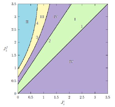
Figure 7: (Color online) Regions of operation modes in the $J_{z}^{i}$-$J_{z}^{f}$ plane for quantum Otto thermal machine with $R_{1}=0.7$, $R_{2}=2$ and bath temperatures $T_{c}=1$ and $T_{h}=1.5$: I (green), engine; II (blue), refrigerator; III (yellow), heater; IV (violet), accelerator. Lines 1–4 are the boundaries separating the listed regions

Regions corresponding to different modes of operation are marked here with Roman numerals and additionally colored. The boundaries separating the regions are marked with Arabic numerals 1-4. It is noteworthy that curves 3 and 4 do not intersect each other and do not intersect lines 1 and 2.

Finding the signs of $Q_{c}$, $W$ and $Q_{h}$ in each such region made it possible to determine that there are only four different types of regions, see again Fig. 7. Firstly, the region I with $Q_{c}<0$, $W<0$ and $Q_{h}>0$ naturally corresponds to engine mode, which is denoted as $\{\leftarrow\uparrow\leftarrow\}$. Secondly, the region II with $Q_{c}>0$, $W>0$ and $Q_{h}<0$, which is identified with a refrigerator or heat pump, and for clarity we depict it in the form $\{\rightarrow\downarrow\rightarrow\}$. Then the region III, where $W>0$ and both $Q_{h}$ and $Q_{c}$ are less than zero; this is a heater that is represented as $\{\leftarrow\downarrow\rightarrow\}$. Finally, the region IV in which $W$ and $Q_{h}$ are grater than zero while $Q_{c}<0$, that is $\{\leftarrow\downarrow\leftarrow\}$; this is the so-called accelerator or cold-bath heater GK96 ; S21 ; CRAOR22 .

The total work output $W(J_{z}^{i},J_{z}^{f})$, Eq. (4.3), has a local minimum $W_{min}=-0.030259$ at the point $(0.659225,0.976325)$. The hot heat (4.3) at this point is $Q_{h}=0.343863$. Therefore, in accord with Eq. (14), the efficiency at maximal power equals $\eta_{mp}=8.8\%$. This value is less than Novikov’s efficiency equal to $18.4\%$.

A similar scheme of regions for the operating modes is shown in Fig. 8.

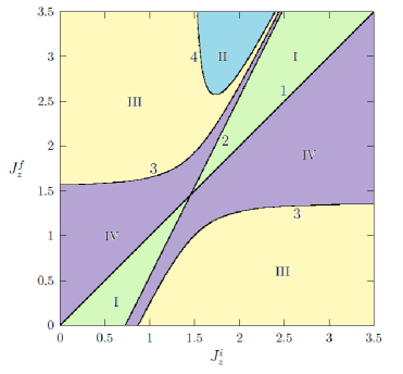
Figure 8: (Color online) Operation modes for a quantum Otto cycle in the plane $J_{z}^{i}$-$J_{z}^{f}$. The regions corresponding to each operation mode are marked as I, heat engine - green; II, refrigerator - blue; III, heater - yellow; and IV, accelerator - violet. Lines 1 and 2 are the boundaries $W=0$, while the curves 3 and 4 result from conditions $Q_{h}=0$ and $Q_{c}=0$, respectively. Straight lines 1 and 2 are the boundaries $W=0$, and curves 3 and 4 follow from the conditions $Q_{h}=0$ and $Q_{c}=0$, respectively. Parameters $R_{1}=3$ and $R_{2}=0.05$. Temperatures of thermal reservoirs are $T_{c}=1$ and $T_{h}=2$

It corresponds to the following parameter values: $R_{1}=3$, $R_{2}=0.05$, $T_{c}=1$, and $T_{h}=2$. According to Eqs. (50) and (51), the boundaries 1 and 2 intersect at the point $(1.45295,1.45295)$. Above this point, the total work output has minimumal value of $W=-0.044432$ at the point $(2.79285,3.35601)$. The heat $Q_{h}$ at this point equals 0.168719. Therefore the efficiency of heat engine is 26.3$\%$. Moreover, below of the intersection point, the work $W(J_{z}^{i},J_{z}^{f})$ has the second local minimum. It is located at $(-0.104884,-0.762864)$ and equals $W=-0.119575$. Here $Q_{h}=0.63495$ and hence $\eta_{mp}=18.8\%$. Both these efficiencies are less than $\eta_{N}=29.3\%$.

Next, Fig. 9 shows the operating mode areas for the following parameters: $R_{1}=1.3$, $R_{2}=0.8$, $T_{c}=1$, and $T_{h}=2.5$.

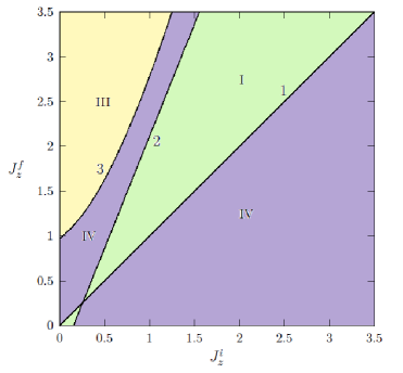
Figure 9: (Color online) The same as in Figs. 7 and 8, but for $R_{1}=1.3$, $R_{2}=0.8$, $T_{c}=1$ and $T_{h}=2.5$

The picture here is similar to the previous two cases.

Concluding this subsection, we can state the following. Only four different operating modes were observed for the thermal machine under study. They are listed in Table 2.

Table 2: Operating modes of the Otto machine depending on signs $Q_{c}$, $W$ and $Q_{h}$

mode	$Q_{c}$	$W$	$Q_{h}$	scheme
engine	$-$	$-$	$+$	$\{\leftarrow\uparrow\leftarrow\}$
refrigerator	$+$	$+$	$-$	$\{\rightarrow\downarrow\rightarrow\}$
heater	$-$	$+$	$-$	$\{\leftarrow\downarrow\rightarrow\}$
accelerator	$-$	$+$	$+$	$\{\leftarrow\downarrow\leftarrow\}$

Although there are eight ($2^{3}=8$) different combinations of signs for $Q_{c}$, $W$ and $Q_{h}$, the regimes $\{\rightarrow\downarrow\leftarrow\}$ and $\{\leftarrow\uparrow\rightarrow\}$ are prohibited by the first law of thermodynamics (12). Moreover, as noted in Ref. ZLCL07 , the variants ($Q_{c}>0,W>0,Q_{h}<0$) and ($Q_{c}>0,W>0,Q_{h}>0$), or in our notation $\{\rightarrow\uparrow\rightarrow\}$ and $\{\rightarrow\uparrow\leftarrow\}$, contradict the second law of thermodynamics ($\oint\delta Q/T\geq 0$ or $dS\geq 0$). As seen from Figs. 7–9, the operating mode regions alternate in the following order: engine-accelerator-heater-refrigerator.

5 Concluding remarks

In the present paper, we have examined a two-qubit Heisenberg XYZ model with DM and KSEA interactions under a non-uniform external magnetic field as the working substance of a quantum Otto thermal machine. Equations (19) and (20) show, firstly, that the KSEA interaction affects the operation of the machine only through the collective parameter $R_{1}$, and DM interaction only through $R_{2}$, and secondly, the roles of DM and KSEA interactions change places when the longitudinal exchange constant $J_{z}$ changes the antiferromagnetic behavior to ferromagnetic.

Combining analytical and numerical analysis, we have found regions in the parameter space for possible operating modes of the thermal machine. Only such four modes as a heat engine, refrigerator (heat pump), heater or dissipator (when work is converted into the heat of both baths at once) and a thermal accelerator or cold-bath heater (fast defrost regime) are acceptable.

The engine and refrigerator mode regions can directly border each other (Fig. 4) or they are separated by areas with accelerator and heater regimes (Figs. 7 and 8).

We have found and investigated the efficiency of the heat engine at maximum output power. Remarkably, cases have been discovered where there are two local extrema of the total work; their appearance is due to splitting the engine mode region into two subregions. Optimal efficiency has been observed not only less than the Novikov efficiency, but also greater than it for certain choices of model parameters. However, the Carnot efficiency was never exceeded.

Acknowledgment Two of us, E. K. and M. Yu., were supported by the program CITIS #AAAA-A19-119071190017-7.

References

- (1) Basov, N.G., Prokhorov, A.M.: Possible methods of obtaining active molecules for a molecular oscillator. ZhETF 28, 249 (1955) [in Russian]
- (2) Basov, N.G., Prokhorov, A.M.: Possible methods of obtaining active molecules for a molecular oscillator. Sov. Phys. JETP 1, 184 (1955) [in English]
- (3) Basov, N.G., Prokhorov, A.M.: Molecular generator and amplifier. Usp. Fiz. Nauk 57, 485 (1955) [in Russian]
- (4) Bloembergen, N.: Proposal for a new type solid state maser. Phys. Rev. 104, 324 (1956)
- (5) Scovil, H.E.D., Feher, G., Seidel, H.: Operation of a solid state maser. Phys. Rev. 105, 762 (1957)
- (6) Zverev, G.M., Kornienko, L.S., Manenkov, A.A., Prokhorov, A.M.: A chromium corundum paramagnetic amplifier and generator. ZhETF 34, 1660 (1958) [in Russian]
- (7) Zverev, G.M., Kornienko, L.S., Manenkov, A.A., Prokhorov, A.M.: A chromium corundum paramagnetic amplifier and generator. Sov. Phys. - JETP 7, 1141 (1958) [in English]
- (8) Maiman, T.H.: Stimulated optical radiation in ruby. Nature 187, 493 (1960)
- (9) Scovil, H.E.D., Schulz-DuBois, E.O.: Three-level masers as heat engines. Phys. Rev. Lett. 2, 262 (1959)
- (10) Geusic, J.E., Schulz-DuBios, E.O., Scovil, H.E.D.: Quantum equivalent of the Carnot cycle. Phys. Rev. 156, 343 (1967)
- (11) Geva, E., Kosloff, R.: Three-level quantum amplifier as a heat engine: A study in finite-time thermodynamics. Phys. Rev. E 49, 3903 (1994)
- (12) Geva, E., Kosloff, R.: The quantum heat engine and heat pump: An irreversible thermodynamic analysis of the three-level amplifier. J. Chem. Phys. 104, 7681 (1996)
- (13) Li, S.-W., Kim, M.B., Agarwal, G.S., Scully, M.O.: Quantum statistics of a single-atom Scovil–Schulz-DuBois heat engine. Phys. Rev. A 96, 063806 (2017)
- (14) Ghosh, A., Gelbwaser-Klimovsky, D., Niedenzu, W., Lvovsky, A.I., Mazets, I., Scully, M.O., Kurizki, G.: Two-level masers as heat-to-work converters. Proc. Natl. Acad. Sci. U.S.A. 115, 9941 (2018)
- (15) Singh, V.: Optimal operation of a three-level quantum heat engine and universal nature of efficiency. Phys. Rev. Res. 2, 043187 (2020)
- (16) Carnot, S.: Rflexions sur la Puissance Motrice du Feu et sur les Machines propres Dvelopper cette Puissance. Bachelier, Paris (1824)
- (17) Vinjanampathy, S., Anders, J.: Quantum thermodynamics. Contemp. Phys. 57, 545 (2016)
- (18) Thermodynamics in the Quantum Regime. Fundamental Aspects and New Directions. Binder, F., Correa, L.A., Gogolin, C., Anders, J., Adesso, G. (eds.). Springer, Berlin (2018)
- (19) Deffner, S., Campbell, S.: Quantum Thermodynamics. An introduction to the thermodynamics of quantum information. Morgan & Claypool, San Rafael, CA, USA (2019); arXiv:1907.01596v1 [quant-ph]
- (20) Ghosh, A., Mukherjee, V., Niedenzu, W., Kurizki, G.: Are quantum thermodynamic machines better than their classical counterparts? Eur. Phys. J. Spec. Top. 227, 2043 (2019)
- (21) Myers, N.M., Abah, O., Deffner, S.: Quantum thermodynamic devices: from theoretical proposals to experimental reality. AVS Quantum Sci. 4, 027101 (2022)
- (22) Alicki, R., Kosloff, R.: Introduction to quantum thermodynamics: History and prospects. In: Thermodynamics in the Quantum Regime. Fundamental Aspects and New Directions. Binder, F., Correa, L.A., Gogolin, C., Anders, J., Adesso, G. (eds.). Springer, Berlin (2018).
- (23) Quan, H.T., Liu, Y.-x., Sun, C.P., Nori, F.: Quantum thermodynamic cycles and quantum heat engines. Phys. Rev. E 76, 031105 (2007)
- (24) Quan, H.T.: Quantum thermodynamic cycles and quantum heat engines. II. Phys. Rev. E 79, 041129 (2009)
- (25) Pea, F.J., Negrete, O., Corts, N., Vargas, P.: Otto engine: classical and quantum approach. Entropy 22, 755 (2020)
- (26) Zhang, G.-F.: Entangled quantum heat engines based on two two-spin systems with Dzyaloshinski-Moriya anisotropic antisymmetric interaction. Eur. Phys. J. D 49, 123 (2008)
- (27) Zhao, L.-M., Zhang, G.-F.: Entangled quantum Otto heat engines based on two-spin systems with the Dzyaloshinski–Moriya interaction. Quantum Inf. Process. 16:216 (2017)
- (28) Ahadpour, S., Mirmasoudi, F.: Coupled two-qubit engine and refrigerator in Heisenberg model. Quantum Inf. Process. 20:63 (2021)
- (29) Yurischev, M.A.: On the quantum correlations in two-qubit XYZ spin chains with Dzyaloshinsky–Moriya and Kaplan–Shekhtman–Entin-Wohlman–Aharony interactions. Quantum Inf. Process. 19:336 (2020)
- (30) Fedorova, A.V., Yurischev, M.A.: Quantum entanglement in the anisotropic Heisenberg model with multicomponent DM and KSEA interactions. Quantum Inf. Process. 20:169 (2021)
- (31) Kieu, D.: The second law, Maxwell’s demon, and work derivable from quantum heat engines Phys. Rev. Lett. 93, 140403 (2004)
- (32) Born, M.: Das Adiabatenprinzip in der Quantenmechanik. Z. Phys. 40, 167 (1927)
- (33) Born, M., Fock, V.: Beweis des Adiabatensatzes. Z. Phys. 51, 165 (1928)
- (34) Messiah, A.: Quantum Mechanics. Dover, New York (1999)
- (35) Quan, H.T., Zhang, P., Sun, C.P.: Quantum heat engine with multi-level quantum systems. Phys. Rev. E 72, 056110 (2005)
- (36) Levy, A., Gelbwaser-Klimovsky, D.: Quantum features and signatures of quantum thermal machines. In: Thermodynamics in the Quantum Regime. Fundamental Aspects and New Directions. Binder, F., Correa, L.A., Gogolin, C., Anders, J., Adesso, G. (eds.). Springer, Berlin (2018).
- (37) Il’in, N., Aristova, A., Lychkovskiy, O.: Adiabatic theorem for closed quantum systems initialized at finite temperature. Phys. Rev. A 104, 030202 (2021)
- (38) Singh, A., Benjamin, C.: Magic angle twisted bilayer graphene as a highly efficient quantum Otto engine. Phys. Rev. B 104, 125445 (2021)
- (39) Feynman, R.P., Leighton, R.B., Sands, M.: The Feynman lectures on physics, Vol. 1. Addison-Wesley, Reading, Mass. (1964, second printing)
- (40) Novikov, I.I.: The efficiency of atomic power stations. Atomnaya Energiya 3, 409 (1957) [in Russian]
- (41) Novikov, I.I.: The efficiency of atomic power stations. J. Nucl. Energy (1954) 7, 125 (1958)
- (42) Vukalovich, M.P., Novikov, I.I.: Termodinamika. Mashinostroenie, Moskva (1972) [in Russian]
- (43) Curzon, F.L., Ahlborn, B.: Efficiency of a Carnot engine at maximum power output. Am. J. Phys. 43, 22 (1975)
- (44) Ahlborn, B., Curzon, F.L.: Time scales for energy transfer. J. Non-Equilib. Thermodyn. 29, 301 (2004)
- (45) Vaudrey, A., Lanzetta, F., Feidt, M.: H. B. Reitlinger and the origins of the efficiency at maximum power formula for heat engines. J. Non-Equilib. Thermodyn. 39, 199 (2014)
- (46) Feidt, M.: The history and perspectives of efficiency at maximum power of the Carnot engine. Entropy 19, 369 (2017)
- (47) Hoffmann, K.H.: An introduction to endoreversible thermodynamics. Atti dell’Accademia Peloritana dei Pericolanti Classe di Scienze Fisiche, Matematiche e Naturali, Vol. LXXXVI, C1S0801011 (2008) - Suppl. 1; DOI:10.1478/C1S0801011
- (48) Smith, Z., Pal, P.S., Deffner. S.: Endoreversible Otto engines at maximal power. J. Non-Equilib. Thermodyn. 45, 305 (2020)
- (49) Sacchi, M.F.: Multilevel quantum thermodynamic swap engines. Phys. Rev. A 104, 012217 (2021)
- (50) Cruz, C., Rastegar-Sedehi, H.-R., Anka, M.F., de Oliveira, T.R., Reis, M.: Quantum Stirling engine based on dinuclear metal complexes. ArXiv:2208.14548v1 (2022)
- (51) Zhang, T., Liu, W.-T., Chen, P.-X., Li, C.-Z.: Four-level entangled quantum heat engines. Phys. Rev. A 75, 062102 (2007)