Motion of Stars in Layered Inhomogeneous Elliptical Galaxies S. A. Gasanov Sternberg Astronomical Institute, Moscow State University, Moscow, Russia e-mail: gasanovsa57@gmail.com

Abstract. The problem of the spatial motion of a passively gravitating body (PGB) in the gravitational field of a layered inhomogeneous elliptical galaxy (LIEG) is considered on the basis of the previously developed model. It is assumed that a LIEG consists of baryonic mass (BM) and dark matter (DM), which have differ- ent laws of density distribution. A star or the center of mass of a globular cluster is taken as the PGB, the motion of which considers the BM and DM attraction. To obtain accurate results, the BM and DM attraction potentials are not expanded in a series, but their exact expressions are taken. An analogue of the Jacobi inte- gral is found, the region of the possible motion of the PGB is determined, and the zero-velocity surfaces are constructed. The stationary solutions (libration points) are found to be stable in the sense of Lyapunov. The results are applied to the elliptical galaxies NGC 4472 (M 49), NGC 4697, and NGC 4374 (M 84).

Keywords: elliptical galaxy, baryonic mass, dark matter, analogue of the Jacobi integral, libration points, sta- bility in the sense of Lyapunov

1. INTRODUCTION

The problem of the spatial motion of a passively gravitating body (PGB) in the gravitational field of an elliptical galaxy (EG) according to models 1 and 2 is considered in [1, 2]. A similar problem of the PGB motion inside (near) a globular cluster (GC) belonging to an EG is studied in [3]. The results obtained in [1–3] are applied to model elliptical galaxies with parameters that exactly coincide with the parameters of the elliptical galaxies NGC 4472 (M 49), NGC 4697, and NGC 4374 (M 84); these results are presented in the form of figures and atable. Three new EG models (Models 3, 4, and 5) are considered in [4]. Of greatest interest is Model 5, according to which the EG with a halo (option 1) or without it (option 2) is represented as an inhomogeneous ellipsoid of revolution, i.e., an elongated spheroid that consists of BM and DM. Such a spheroid was chosen as a model of a triaxial EG because its dynamic properties are very close to those of a triaxial ellipsoid [5]. In addition, the fulfillment of the potential matching conditions should not be considered in Model 5, since there is no interface between the BM and DM in the galaxy. The results obtained in [4] are applied to sixty EGs and are presented in the form of tables for ten of them. The models mentioned above are intended for solving problems of celestial mechanics and partially astrophysics. Another attempt to study the impact of the DM on the kinematics and dynamics of PGB is made within the context of these models. These models cannot claim to provide a complete coverage of the DM problem as a whole. Moreover, according to some authors [6], the bulk of the DM lies outside the luminous part of an elliptical galaxy, while others believe [7, 8] that the DM content in the inner regions of an EG is comparable to the BM content. This study considers the problem of the spatial motion of a PGB in the gravitational field of an LIEG that has the shape of an elongated spheroid. Model 5 is used as the basis. An analogue of the Jacobi integral is found, the region of the possible motion of the PGB is determined, and the zero-velocity surfaces are constructed. The stationary solutions (libration points) are found to be stable in the sense of Lyapunov. The question of equilibrium and stability of the dynamical system studied in Model 5 will be considered separately in another paper of the author.

2. STATEMENT OF THE PROBLEM. EQUATIONS OF MOTION

Let us consider the problem of the spatial motion of a PGB in the LIEG gravitational field according to Model 5 in the coordinate system $OXYZ$. The conditional boundaries of such a galaxy are determined by the $D_{25}$ and $R_{25}$ values [9]. $OXYZ$ is a coordinate system with the origin at the center of the EG rotating at a constant angular velocity $\Omega$ around the polar axis $OZ$ and with axes directed along the corresponding principal axes of the EG. The rectangular coordinates $(x,y,z)$ of the PGB in this coordinate system are determined from the system of equations [10]

$$\frac{d^{2}x}{dt^{2}}-2\Omega\,\frac{dy}{dt}=\frac{\partial U}{\partial x},\quad\frac{d^{2}y}{dt^{2}}+2\Omega\,\frac{dx}{dt}=\frac{\partial U}{\partial y},\quad\frac{d^{2}z}{dt^{2}}=\frac{\partial U}{\partial z}$$

Here, the force function $U=U\,(x,y,z)$ is defined by the equality

$$U=\frac{\Omega^{2}}{2}\,(x^{2}+y^{2})+V,\quad V=U^{*}+U_{G},$$

where the first term is the centrifugal force potential, $V=V\,(x,y,z)$ is the potential of the force of attraction, and function $U$ can be considered the potential of gravity. $U^{*}=U^{*}(x,y,z)$ and $U_{G}=U_{G}(x,y,z)$ are the potentials of the LIEG’s BM and DM, respectively, the explicit form of which is given in the following sections.

For an inhomogeneous EG to exist as a figure of equilibrium, the necessary condition of the Poincare inequality for the angular velocity of rotation [11] must be satisfied:

$$\Omega^{2}\leq 2\pi G\bar{\rho},\quad(\Omega^{2}\leq\pi G\rho_{0},\quad\Omega^{2}\leq 0.4\pi G\bar{\rho})$$

Here, $G$ is the gravitational constant, and $\bar{\rho}$ is the average density of an inhomogeneous elliptical galaxy. The fulfillment of the Poincare inequality guarantees that the total force of gravity is oriented inward and the pressure is non-negative. The stricter Crudeli and Kondratyev inequalities [12] are indicated in parentheses. In the Crudeli inequality, $\rho_{0}$ is the density in the center of the galaxy and it decreases from the center to the periphery. In addition, the direction of gravity is not involved.

Obviously, the system of equations (1) allows an analogue of the Jacobi integral in the form [1, 2, 10]

$$\left(\frac{dx}{dt}\right)^{2}+\left(\frac{dy}{dt}\right)^{2}+\left(\frac{dz}{dt}\right)^{2}=2U-2C,\quad C=\mbox{const},$$

from which zero-velocity surfaces and the region of possible motion of the PGB are easily obtained:

$$U=C,\qquad U\geq C$$

respectively, where $C$ is the analogue of the Jacobi constant.

3. BARYONIC MASS POTENTIAL OF A LAYERED INHOMOGENEOUS ELLIPTICAL GALAXY

We will assume that the LIEG has the form of an inhomogeneous elongated spheroid bounded by a spheroidal surface,

$$\frac{x^{2}}{a^{2}}+\frac{w^{2}}{c^{2}}=m^{2},\quad w^{2}=y^{2}+z^{2},\qquad(a\geq b=c,\quad 0\leq m\leq 1),$$

where the value of the family parameter $m=0$ corresponds to the center of the LIEG, and $m=1$ to its outer border. The distribution laws of density $\rho\,(m)$ and surface brightness $I\,(m)$ of the BM are described by the expressions [3, 13, 14]

$$\rho\,(m)=\frac{\rho_{0}}{\left(1+\displaystyle\beta m^{2}\right)^{3/2}},\quad I\,(m)=\frac{I_{0}}{1+\displaystyle\beta m^{2}}$$

respectively. Here, $\rho_{0}$ is the density of the center (core) of an elliptical galaxy, $m$ is the parameter of the family of ellipsoidal surfaces (5) that comprise its luminous part, and parameter $\beta\gg 1$ is selected separately for each EG [13] and is found by aligning the photometry data [12, 13]. $I_{0}$ is the central surface brightness. The profile in the form (5) will be called ”astrophysical” in accordance with [12]; it is consistent with modern concepts of the EG structure [13, 14].

The attraction potential of the LIEG BM with density $\rho\,(m)$ to the outer point $P=P\,(x,y,z)$ and its derivatives with respect to the coordinate axes are determined by the equalities [10, 12]

$$U^{*}(P)=\pi Gac^{2}\int\limits_{\lambda}^{\infty}\frac{\delta\,(m^{2}(u))}{\Delta\,(u)}\,du,\quad\frac{\partial U^{*}(P)}{\partial R}=-\,2\pi Gac^{2}\,R\,\int\limits_{\lambda}^{\infty}\frac{\rho\,(m^{2}(u))\,du}{(A^{2}+u)\,\Delta\,(u)},$$

where $R$ is one of the coordinates $\{x,y,z\}$, and $A^{2}=\{a^{2},c^{2}\}$. If the BM profile is determined by equality (5),

$$\delta\,(m^{2}(u))=\int\limits_{m^{2}(u)}^{1}\rho\,(v)dv^{2}=\frac{2\rho_{0}}{\beta}\,\left[-\,\frac{1}{\displaystyle\sqrt{1+\beta}}+\frac{1}{\displaystyle\sqrt{1+\beta\,m^{2}(u)}}\right],$$

$$m^{2}(u)=\frac{x^{2}}{a^{2}+u}+\frac{w^{2}}{c^{2}+u},\quad\Delta^{2}(u)=(a^{2}+u)(c^{2}+u)^{2},\quad m^{2}(0)=\frac{x^{2}}{a^{2}}+\frac{w^{2}}{c^{2}}>1,$$

and the fulfillment of the condition $m^{2}(0)>1$ for the coordinates of the outer point $P$ of the luminous part of the EG is mandatory. Parameter $\lambda$ is the positive root of the quadratic equation $m^{2}(\lambda)=1$:

$$\lambda^{2}+p\lambda+q=0,\quad\lambda=\frac{1}{2}\,\left(-\,p+\sqrt{\delta}\right),\quad\delta=p^{2}-4q>0,$$

where

$$p=a^{2}+c^{2}-x^{2}-w^{2},\quad q=a^{2}c^{2}\left(1-\frac{x^{2}}{a^{2}}-\frac{w^{2}}{c^{2}}\right)=a^{2}c^{2}\left[1-m^{2}(0)\right]<0$$

By virtue of (7), for $p>0$, we have

$$c^{2}m^{2}(0)<x^{2}+w^{2}<a^{2}m^{2}(0),\quad a^{2}+c^{2}-a^{2}m^{2}(0)<p<a^{2}+c^{2}-c^{2}m^{2}(0)$$

Obviously, the potential $U^{*}$ is a function of parameter $\lambda$, which, in turn, depends on the coordinates of the outer point $P=P\,(x,y,z)$. After calculating the integral in (6) for the outer potential, we obtain

$$U^{*}(P)\equiv U^{*}(\lambda)=\frac{2\pi G\rho_{0}ac^{2}}{\beta}\,\left[-\,\frac{U_{1}(\lambda)}{\displaystyle\sqrt{1+\beta}}+U_{2}(\lambda)\right],$$

where

$$U_{1}(\lambda)=\int\limits_{\lambda}^{\infty}\frac{du}{\displaystyle(c^{2}+u)\,\sqrt{a^{2}+u}}=\frac{\ln\varphi\,(\lambda)}{\displaystyle\sqrt{a^{2}-c^{2}}},\quad\varphi\,(\lambda)=\frac{\displaystyle\sqrt{a^{2}+\lambda}+\sqrt{a^{2}-c^{2}}}{\displaystyle\sqrt{a^{2}+\lambda}-\sqrt{a^{2}-c^{2}}},$$

$$U_{2}(\lambda)=\int\limits_{\lambda}^{\infty}\frac{du}{\displaystyle\displaystyle(c^{2}+u)\,\sqrt{a^{2}+u}\,\sqrt{1+\beta\,m^{2}(u)}}=\int\limits_{\lambda}^{\infty}\frac{du}{\displaystyle\sqrt{c^{2}+u}\,\sqrt{(u-v_{1})(u-v_{2})}}=\frac{2F\,(\alpha,n)}{\displaystyle\sqrt{-\,c^{2}-v_{2}}}$$

Here,

$$v_{1}=\frac{-\,p_{1}+\sqrt{\delta_{1}}}{2}<0,\quad v_{2}=\frac{-\,p_{1}-\sqrt{\delta_{1}}}{2}<0,\quad\delta_{1}=p_{1}^{2}-4q_{1}>0,$$

$$p_{1}=a^{2}+c^{2}+\beta\,(x^{2}+w^{2})>0,\quad q_{1}=a^{2}c^{2}\left(1+\beta\,\frac{x^{2}}{a^{2}}+\beta\,\frac{w^{2}}{c^{2}}\right)>0,$$

and

$$v_{1}+v_{2}=-\,p_{1}<0,\quad v_{1}v_{2}=q_{1}>0,\quad c^{2}+v_{2}<c^{2}+v_{1}<0,\quad(0>v_{1}>v_{2})$$

Argument $\alpha$ and modulus $n$ of an incomplete elliptic integral of the first kind $F\,(\alpha,n)$ are

$$\alpha=\displaystyle\sqrt{\frac{-\,c^{2}-v_{2}}{\lambda-v_{2}}},\quad n=\sqrt{\displaystyle\frac{v_{1}-v_{2}}{-c^{2}-v_{2}}}<1$$

At the origin of coordinates (in the center of the galaxy), it is obvious that the value of the potential $U^{*}(\lambda)$ considering the equalities

$$x=0,\quad w=0,\quad m=0,\quad m^{2}(u)=0,\quad\lambda=0,\quad\rho\,(m=0)=\rho_{0},\quad U_{2}(\lambda)\equiv U_{1}(\lambda)$$

will be

$$U_{0}^{*}=\frac{2\pi G\rho_{0}ac^{2}}{\beta}\,\frac{\ln\varphi\,(0)}{\displaystyle\sqrt{a^{2}-c^{2}}}\,\left(1-\frac{1}{\displaystyle\sqrt{1+\beta}}\right),\quad\varphi\,(0)=\varphi\,(\lambda=0),$$

and function $\varphi\,(\lambda)$ is defined above.

The last equality can also be obtained from expression (8) of the potential $U^{*}(\lambda)$ setting $U_{2}(\lambda)=U_{1}(\lambda)$ and $\lambda=0$.

Setting $z=0,x\neq 0$, and $w=y\neq 0$ in the corresponding expressions, we find the parameter $\lambda$, the roots $v_{1}$ and $v_{2}$, then the values of the functions $U_{1}(\lambda)$ and $U_{2}(\lambda)$. Further, we obtain the expression for the potential $U^{*}(\lambda)$ in the plane $Oxy$. Similarly, at $y=0$, $x\neq 0$, $w=z\neq 0$, we find the expression for potential $U^{*}(\lambda)$ in the plane $OXZ$.

Further, in the plane $OYZ$ we have

$$x=0,\quad m^{2}(u)=\frac{w^{2}}{c^{2}+u},\quad\lambda=w^{2}-c^{2},\quad v_{1}=-\,a^{2},\quad v_{2}=-\,c^{2}-\beta w^{2}$$

The potential $U^{*}(\lambda)$ will then be described by exactly the same equality as (8) with the only difference that the parameter $\lambda$ and function $U_{2}(\lambda)$ are defined differently:

$$U_{2}(\lambda)=\frac{2F\,(\alpha_{0},n_{0})}{\displaystyle\sqrt{h^{2}-c^{2}}},\quad\alpha_{0}=\displaystyle\sqrt{\frac{h^{2}-c^{2}}{\lambda+h^{2}}},\quad n_{0}=\displaystyle\sqrt{\frac{h^{2}-a^{2}}{h^{2}-c^{2}}},\quad h^{2}=\beta w^{2}+c^{2}$$

Here, $\alpha_{0}$ and $n_{0}$ are the argument and modulus of an incomplete elliptic integral of the first kind $F\,(\alpha_{0},n_{0})$.

The derivative from the potential $U^{*}(\lambda)$ with respect to according to (6) is

$$\frac{\partial U^{*}(\lambda)}{\partial w}=-\,2\pi G\rho_{0}ac^{2}w\,\int\limits_{\lambda}^{\infty}\frac{du}{\displaystyle\sqrt{(h^{2}+u)^{3}(a^{2}+u)(c^{2}+u)}}=-\,\frac{4\pi G\rho_{0}ac^{2}}{\displaystyle(h^{2}-a^{2})\,\sqrt{\beta}}\,\left[F\,(\alpha_{0},n_{0})-E\,(\alpha_{0},n_{0})\right],$$

where $F\,(\alpha_{0},n_{0})$ and $E\,(\alpha_{0},n_{0})$ are incomplete elliptic integrals of the first and second kind, respectively. The $\alpha_{0}$, $n_{0}$ and $h^{2}$ values are defined above. Setting in these formulas $z=0$ or $y=0$, we obtain the expressions for the potential $U^{*}(\lambda)$ and its derivative on the coordinate axes $OY$ or $OZ$, respectively. It is taken into account that $x=0$.

Finally, on the coordinate axis $OX$, we have

$$w=0,\quad m^{2}(u)=\frac{x^{2}}{a^{2}+u},\quad\lambda=x^{2}-a^{2},\quad v_{1}=-\,c^{2},\quad v_{2}=-\,a^{2}-\beta x^{2}$$

In this case, expression (8) of the potential $U^{*}(\lambda)$ should take into account that

$$U_{2}(\lambda)=\int\limits_{\lambda}^{\infty}\frac{du}{\displaystyle\displaystyle(c^{2}+u)\,\sqrt{a^{2}+u}\,\sqrt{1+\beta\,m^{2}(u)}}=\int\limits_{\lambda}^{\infty}\frac{du}{\displaystyle(c^{2}+u)\,\sqrt{p^{2}+u}}=\frac{\ln\varphi_{1}(\lambda)}{\displaystyle\sqrt{p^{2}-c^{2}}},$$

where

$$\varphi_{1}(\lambda)=\displaystyle\frac{\displaystyle\sqrt{p^{2}+\lambda}+\sqrt{p^{2}-c^{2}}}{\displaystyle\sqrt{p^{2}+\lambda}-\sqrt{p^{2}-c^{2}}},\quad p^{2}=a^{2}+\beta x^{2}$$

The derivative from the potential $U^{*}(\lambda)$ with respect to $x$ has the form

$$\frac{\partial U^{*}(\lambda)}{\partial x}=-\,2\pi G\rho_{0}ac^{2}x\,\int\limits_{\lambda}^{\infty}\frac{du}{\displaystyle(c^{2}+u)\,\sqrt{(p^{2}+u)^{3}}}=\frac{2\pi G\rho_{0}ac^{2}x}{p^{2}-c^{2}}\,\left[\frac{2}{\displaystyle\sqrt{p^{2}+\lambda}}-\frac{\ln\varphi_{1}(\lambda)}{\displaystyle\sqrt{p^{2}-c^{2}}}\right]$$

The function $\varphi_{1}(\lambda)$ and parameter $p^{2}$ are defined above.

Now let us calculate the derivatives of the potential $U^{*}(\lambda)$ with respect to the coordinates in the general case:

$$\frac{\partial U^{*}(\lambda)}{\partial R}=-\,2\pi G\rho_{0}ac^{2}R\,\bar{R}\,(\lambda),\quad R=\{x,y,z\},\quad\bar{R}\,(\lambda)=\{X\,(\lambda),Y\,(\lambda),Z\,(\lambda)\},$$

where

$$X\,(\lambda)=\int\limits_{\lambda}^{\infty}\frac{c^{2}+u}{\displaystyle\sqrt{c^{2}+u}\,\sqrt{(u-v_{1})^{3}(u-v_{2})^{3}}}\,du=S_{0}X_{0}(\lambda)+S_{1}(\lambda),$$

$$Y\,(\lambda)=Z\,(\lambda)=\int\limits_{\lambda}^{\infty}\frac{a^{2}+u}{\displaystyle\sqrt{c^{2}+u}\,\sqrt{(u-v_{1})^{3}(u-v_{2})^{3}}}\,du=S_{0}W_{0}(\lambda)+S_{1}(\lambda),$$

Here,

$$S_{0}=\frac{2}{(v_{1}-v_{2})^{2}\sqrt{-c^{2}-v_{2}}},\quad S_{1}(\lambda)=\frac{2}{(v_{1}-v_{2})(c^{2}+v_{1})}\displaystyle\sqrt{\frac{\lambda+c^{2}}{(\lambda-v_{1})(\lambda-v_{2})}},$$

$$X_{0}(\lambda)=2(c^{2}+v_{2})E\,(\alpha,n)-(2c^{2}+v_{1}+v_{2})\,F\,(\alpha,n),$$

$$W_{0}(\lambda)=\frac{(a^{2}+c^{2})(v_{1}+v_{2})+2(a^{2}c^{2}+v_{1}v_{2})}{c^{2}+v_{1}}\,E\,(\alpha,n)-(2a^{2}+v_{1}+v_{2})\,F\,(\alpha,n),$$

where the roots $v_{1}$ and $v_{2}$, as well as the argument $\alpha$ and the modulus $n$ of the elliptic integrals of the first and second kind $F\,(\alpha,n)$ and $E\,(\alpha,n)$ are given above.

Further, it can be established that the potential $U^{*}(\lambda)$ defined by formulas (7) or (8) has all the characteristic properties of a force function:

(1) it is a continuous function of coordinates $x,y,z$ throughout the space;

(2) it has continuous first partial derivatives throughout the space; these derivatives have no discontinuity at the boundary of the ellipsoid, which follows from expression (7), in which we should set $\lambda=0$ to obtain the internal potential;

(3) it turns to zero at infinity along with its first partial derivatives;

(4) it satisfies the Laplace equation outside the LIEG gravitating body, and satisfies the Poisson equation inside the gravitating body ($\lambda=0$).

The proof of these properties follows, inter alia, from the characteristics of the profile $\rho\,(m)$, which is a positive, finite, continuous function and has continuous derivatives of the first and second orders. $\delta\,(m^{2}(u))$ is also such a function. Therefore, the improper integrals in formula (7) converge, and the potential $U^{*}(\lambda)$ and its first derivatives with respect to coordinates are finite, continuous functions of their arguments. In addition, if the PGB recedes to infinity, also tends to infinity. Therefore, the force function $U^{*}(\lambda)$ and its first partial derivatives vanish at infinity. The satisfaction of the Laplace and Poisson equations is verified by calculating the partial second-order derivatives of the potential $U^{*}(\lambda)$. The proof of this is omitted for brevity.

4. DARK MATTER POTENTIAL OF A LAYERED INHOMOGENEOUS ELLIPTICAL GALAXY

For brevity and convenience, we will consider only option 2 of Model 5, from which the results of option1 are obtained by elementary substitution. In this case, the external potential of such a galaxy will be deter- mined by the equality $\widetilde{U}\,(\lambda)=U^{*}(\lambda)+U_{G}(\lambda)$. Here, $U^{*}(\lambda)$ represents the BM potential with the profile $\rho\,(m)$ from (5) and is determined by equality (8), and $U_{G}(\lambda)$ is the DM potential with an analogue of the NFW $\rho_{G}(m)$ profile [4, 15]:

$$\rho_{G}(m)=\frac{K}{\xi m(1+\xi m)^{2}},\quad\xi=\displaystyle\frac{\sqrt[3]{ac^{2}}}{r_{s}},$$

where $r_{s}$ is the radius-scale of the galaxy, and the functions $m^{2}(u)$ and $\Delta\,(u)$ are determined by equality (7). Therefore,

$$U_{G}(\lambda)=\pi Gac^{2}\int\limits_{\lambda}^{\infty}\frac{\chi\,(u)}{\Delta\,(u)}\,du,\quad\frac{\partial U_{G}(\lambda)}{\partial R}=-\,2\pi Gac^{2}R\,\int\limits_{\lambda}^{\infty}\frac{\rho_{G}(m\,(u))\,du}{(A^{2}+u)\,\Delta\,(u)}$$

Here, the values $A^{2},\ \lambda$ and function $\Delta\,(u)$ are defined above (see Section 3), and $\chi\,(u)$ is

$$\chi\,(u)=\int\limits_{m^{2}(u)}^{1}\rho_{G}(v)\,dv^{2}=\frac{2K}{\xi^{2}}\left[\frac{1}{1+\xi m\,(u)}-\frac{1}{1+\xi}\right],$$

So the potential $U_{G}(\lambda)$ will take the form

$$U_{G}(\lambda)=\frac{2\pi GKac^{2}}{\xi^{2}}\,\left[J_{1}(\lambda)+J_{2}(\lambda)\right],$$

where

$$J_{1}(\lambda)=-\,\frac{1}{1+\xi}\int\limits_{\lambda}^{\infty}\frac{du}{\Delta\,(u)},\qquad J_{2}(\lambda)=\int\limits_{\lambda}^{\infty}\frac{du}{\left[1+\xi m\,(u)\right]\Delta\,(u)}$$

After integration, we obtain

$$J_{1}(\lambda)=\displaystyle-\,\frac{\ln\varphi\,(\lambda)}{(1+\xi)\sqrt{a^{2}-c^{2}}},\qquad\varphi\,(\lambda)=\frac{\sqrt{a^{2}+\lambda}+\sqrt{a^{2}-c^{2}}}{\sqrt{a^{2}+\lambda}-\sqrt{a^{2}-c^{2}}}$$

$$J_{2}(\lambda)=\frac{1}{u_{1}-u_{2}}\sum_{k=1}^{2}(-1)^{k+1}\left[\sqrt{a^{2}+u_{k}}\,\ln\psi_{k}(\lambda)-\xi\,\sqrt{x^{2}+w^{2}}\,\frac{\displaystyle\sqrt{f\,(u_{k})}}{c^{2}+u_{k}}\,\ln\eta_{k}(\lambda)\right],$$

where

$$u_{1}=\frac{-\,p_{2}+\sqrt{\delta_{2}}}{2}<0,\quad u_{2}=\frac{-\,p_{2}-\sqrt{\delta_{2}}}{2}<0,\quad\delta_{2}=p_{2}^{2}-4q_{2},\quad(0>u_{1}>u_{2}),$$

$$p_{2}=a^{2}+c^{2}-\xi^{2}(x^{2}+w^{2}),\quad q_{2}=a^{2}c^{2}\left[1-\xi^{2}m^{2}(0)\right],\quad u_{0}=\frac{c^{2}x^{2}+a^{2}w^{2}}{x^{2}+w^{2}},\quad(c^{2}<u_{0}<a^{2}),$$

$$\eta_{k}(\lambda)=\displaystyle\frac{2\sqrt{f\,(u_{k})\,f\,(\lambda)}+(c^{2}+u_{k})(u_{0}+\lambda)+(c^{2}+\lambda)(u_{0}+u_{k})}{(\lambda-u_{k})\left[2\sqrt{f\,(u_{k})}+2u_{k}+c^{2}+u_{0}\right]}$$

$$f\,(u)=(u_{0}+u)(c^{2}+u),\qquad\psi_{k}(\lambda)=\displaystyle\frac{\sqrt{a^{2}+\lambda}+\sqrt{a^{2}+u_{k}}}{\sqrt{a^{2}+\lambda}-\sqrt{a^{2}+u_{k}}},\quad(k=1,2),$$

In the plane $OZY$, we have

$$x=0,\quad m^{2}(u)=\frac{w^{2}}{c^{2}+u},\quad\lambda=w^{2}-c^{2}>0$$

In this case, the potential $U_{G}(\lambda)$ is expressed by equality (12), in which the function $J_{1}(\lambda)$ is exactly the same, but the function $J_{2}(\lambda)$ is defined differently:

$$J_{2}(\lambda)=J_{21}(\lambda)-\xi\,wJ_{22}(\lambda),$$

where

$$J_{21}(\lambda)=\int\limits_{\lambda}^{\infty}\frac{du}{(u+h)\,\sqrt{a^{2}+u}}=\displaystyle\frac{1}{\sqrt{a^{2}-h}}\,\ln\frac{\sqrt{a^{2}+\lambda}+\sqrt{a^{2}-h}}{\sqrt{a^{2}+\lambda}-\sqrt{a^{2}-h}},\quad h=c^{2}-\widetilde{\xi}^{2}w^{2},\ (h<c^{2}<a^{2})$$

$$J_{22}(\lambda)=\int\limits_{\lambda}^{\infty}\frac{du}{(u+h)\,\sqrt{(a^{2}+u)(c^{2}+u)}}=\displaystyle\frac{1}{\sqrt{(a^{2}-h)(c^{2}-h)}}\,\times$$

$$\times\,\left[\ln\frac{\left(\sqrt{(a^{2}+\lambda)(c^{2}-h)}+\sqrt{(c^{2}+\lambda)(a^{2}-h)}\right)^{2}}{\lambda+h}-\ln\left(\sqrt{a^{2}-h}+\sqrt{c^{2}-h}\right)^{2}\right]$$

Setting $w=y$ or $w=z$ in the functions $J_{1}(\lambda)$ and $J_{2}(\lambda)$, we obtain the expressions for the potential $U_{G}(\lambda)$ on the coordinate axes $OY$ or $OZ$, respectively.

On the coordinate axis $OX$, we have

$$w=0,\quad m^{2}(u)=\frac{x^{2}}{a^{2}+u},\quad\lambda=x^{2}-a^{2}>0$$

For the function $J_{2}(\lambda)$, we then find

$$J_{2}(\lambda)=\frac{1}{a^{2}-c^{2}-\xi^{2}x^{2}}\,\left[\sqrt{a^{2}-c^{2}}\,\ln\varphi\,(\lambda)-\xi\,\sqrt{x^{2}}\,\ln\frac{\left(\xi\,\sqrt{x^{2}}+\sqrt{a^{2}+\lambda}\right)^{2}}{\lambda+c^{2}}\right]$$

Here, function $\varphi\,(\lambda)$ is defined above. The potential $U_{G}(\lambda)$, in this case, is expressed by equality (12), in which the expression for the function $J_{1}(\lambda)$ remains exactly the same, and $J_{2}(\lambda)$ is defined by equality (16).

Finally, the value of the potential at the origin (in the center of the galaxy) is

$$U_{G}^{0}=U_{G}(\lambda=0)=\frac{2\pi GKac^{2}}{\xi\,(1+\xi)}\,\frac{\ln\varphi\,(\lambda=0)}{\sqrt{a^{2}-c^{2}}},$$

It should be noted that according to option 1 of Model 5, the EG is considered as an inhomogeneous elongated spheroid consisting of the BM and DM with the corresponding $\rho\,(m)$ and $\rho_{G}(m)$ profiles and the halo. If we assume that the LIEG with the halo is bounded by an elongated spheroidal surface with semiaxes $\widetilde{a}>\widetilde{b}=\widetilde{c}$, in expressions (8) and (12) for the potentials $U^{*}(\lambda)$ and $U_{G}(\lambda)$ and their derivatives, $a$, $c$ should be replaced with $\widetilde{a}$, $\widetilde{c}$. Further, we will obtain an explicit expression for the general potential $\widetilde{U}\,(\lambda)=U^{*}(\lambda)+U_{G}(\lambda)$ according to this variant of Model 5, which is not shown for brevity. In addition, there is also no interface between the BM and DM in this variant, i.e., there is no need to determine the conditions for matching the potentials $U^{*}(\lambda)$ and $U_{G}(\lambda)$.

5. STATIONARY SOLUTIONS. LIBRATION POINTS

To find the stationary solutions of the system of equations (1), we set

$$x=x_{0}=\mbox{const},\quad y=y_{0}=\mbox{const},\quad z=z_{0}=\mbox{const},$$

This will give us a system of algebraic equations for finding stationary solutions in the form

$$\frac{\partial U\,(x_{0},y_{0},z_{0})}{\partial x}=0,\quad\frac{\partial U\,(x_{0},y_{0},z_{0})}{\partial y}=0,\quad\frac{\partial U\,(x_{0},y_{0},z_{0})}{\partial z}=0$$

Solving the system of equations (18), we will consider option 1 with a halo and option 2 without a halo of Model 5. The zero solution $x_{0}=0$, $y_{0}=0$ and $z_{0}=0$ of the system of equations (18) corresponds to the central libration point, which we denote by $L_{1}=L_{1}(0,0,0)$. There are two libration points on axes $OX$ and $OY$, specifically, $L_{2}=L_{2}(x_{0},0,0)$ and $L_{3}=L_{3}(-\,x_{0},0,0)$ on axis $OX$, and $L_{4}=L_{4}(0,y_{0},0)$ and $L_{5}=L_{5}(0,-\,y_{0},0)$ on axis $OY$.

Table 1 shows the coordinates (in kpc) of collinear $L_{2},L_{3}$ and triangular $L_{4},L_{5}$ libration points calculated according to options 1 and 2 of Model 5 for three EGs: NGC 4374, NGC 4472, and NGC 4697 considered to be layered inhomogeneous elongated spheroids.

Table 1. Coordinates (kpc) of the collinear $L_{2}(x_{0},0,0)$, $L_{3}(-\,x_{0},0,0)$, and triangular $L_{4}(0,y_{0},0)$, $L_{5}(0,-\,y_{0},0)$ libration points found according to options 1 and 2 of Model 5 for three EGs. The galaxies are considered to be inhomogeneous elongated spheroids with semiaxes $a>b=c$.

Elliptical	Semiaxes, kpc		Options	Libration points
galaxies	$a$	$b=c$		$x_{0}$	$y_{0}$
NGC 4374	19.947	17.373	1)	442.547	441.301
			2)	22.543	22.189
NGC 4472	22.166	18.437	1)	532.375	530.406
			2)	24.735	24.171
NGC 4697	9.991	6.304	1)	508.274	506.522
			2)	11.121	10.583

6. TYPE AND STABILITY OF SINGULAR POINTS

Singular points of the family $U=C$ are the point at which it is impossible to construct a single tangen plane. To determine such points, we obtain a system ofalgebraic equations that exactly coincides with system (18) for determining libration points. Therefore libration points $L_{n}$ are singular points.

To study the type and establish the stability of singular points (libration points), the force function $U$ expanded into a Taylor series in the neighborhood of $L_{n},\ (n=1,2\cdots 5)$, and a family of zero-velocity surfaces $U=C$ is written (see Section 2). Further, the motion of the PGB near these points, which is expressed by a system of differential equations in vari ations, is considered. After that, the characteristi equation of this system is written and, depending o the roots of this equation, the stability of the libratio points in the sense of Lyapunov in the first approx imation (or in the linear setting) is established accord ing to the well-known Lyapunov theorem. The entir procedure is described in detail by the author [2, 3] Thus, for brevity, it is not presented here.

The type and stability of the central libration point $L_{1}(0,0,0)$ are the same in all models: it is an isolated singular point, stable in the sense of Lyapunov in the first approximation and in a nonlinear setting. Collinear libration points $L_{2}$ and $L_{3}$ found according to Models 3, 4, and 5 in this study are conical singular points with a cone axis $OX$ and are unstable in the sense of Lyapunov in the first approximation, while the triangular libration points $L_{4}$ and $L_{5}$ are singular points with a cone axis and are stable. Therefore, if the PGB (e.g., a star) is very close to the triangular libration points $L_{4}$ or $L_{5}$, it will remain there forever, i.e., there is Hill stability.

It should be noted that the studies [16–18] also showed the instability of libration points $L_{2}$ and $L_{3}$, and stability of $L_{4}$ and $L_{5}$ in the sense of Lyapunov. In addition, nonlinear analysis showed that and are stable for most of the initial conditions in the sense of Lebesgue’s measure, excluding only some resonance cases when instability takes place [18].

7. EXAMPLES OF CONSTRUCTING ZERO-VELOCITY SURFACES

The procedure and method for constructing zero- velocity surfaces, or Hill surfaces, are described in detail in the author’s paper [3]. Therefore, we will not dwell on them here. As an example, we take the ellip- tical galaxies NGC 4374 of the E1 type, NGC 4472 of the E2 type, and NGC 4697 of the E4 type, which we assume to be layered inhomogeneous elongated spher- oids with semiaxes $a>b=c$. Below are the values of the key parameters of these galaxies: stellar mass $M^{*}$ and halo mass $M_{h}$ (in solar masses), radius scale $r_{s}$ in kpc, angular velocity of rotation of galaxies $\Omega$ in radians per million years, parameters $\beta$ and $K$ (in solar masses per cubic parsec) calculated by the well-known formula, as well as the values of the semiaxes $a,b=c$ in kpc and density $\rho_{0}$ at the center of the galaxy, expressed in solar masses per cubic parsec:

$NGC4374:M^{\ast }=3.38844\cdot {10}^{11}{M}_{\odot },M_h=1.5674\cdot {10}^{13}{M}_{\odot },\mathrm{\Omega }=0.01386,\beta =1815,$

$$r_{s}=168.80,\quad a=19.947,\quad b=c=17.373,\quad K=0.167\cdot 10^{-3},\quad\rho_{0}=132.71,$$

$NGC4472:M^{\ast }=4.67735\cdot {10}^{11}{M}_{\odot },M_h=2.172\cdot {10}^{13}{M}_{\odot },\mathrm{\Omega }=0.0139,\beta =858,$

$$r_{s}=197.0,\quad a=22.166,\quad b=c=18.437,\quad K=0.1467\cdot 10^{-3},\quad\rho_{0}=50.844,$$

$NGC4697:M^{\ast }=1.4125\cdot {10}^{11}{M}_{\odot },M_h=6.494\cdot {10}^{12}{M}_{\odot },\mathrm{\Omega }=0.02524,\beta =650,$

$$r_{s}=130.5,\quad a=9.991,\quad b=c=6.304,\quad K=0.3459\cdot 10^{-3},\quad\rho_{0}=194.589$$

Figure 1 shows the constructed zero-velocity surfaces with collinear $L_{1},L_{2},L_{3}$ and triangular libration points $L_{4},L_{5}$ for EG NGC 4472 according to Model5 in the plane $x=0$. On the left is option 2 without a halo, and on the right is option 1 with the galactic halo. Coordinates are given in kiloparsecs.

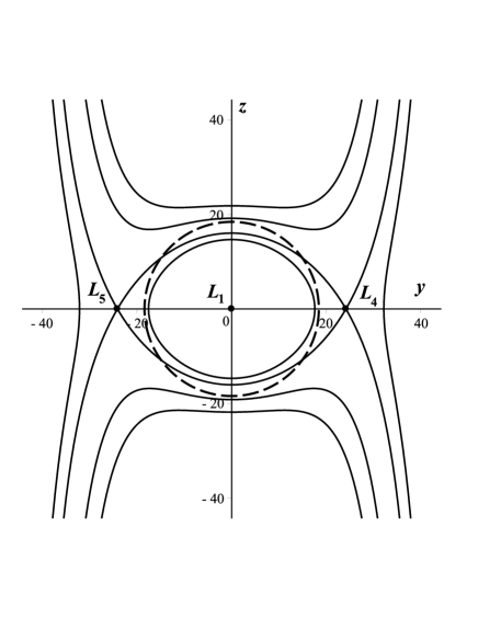
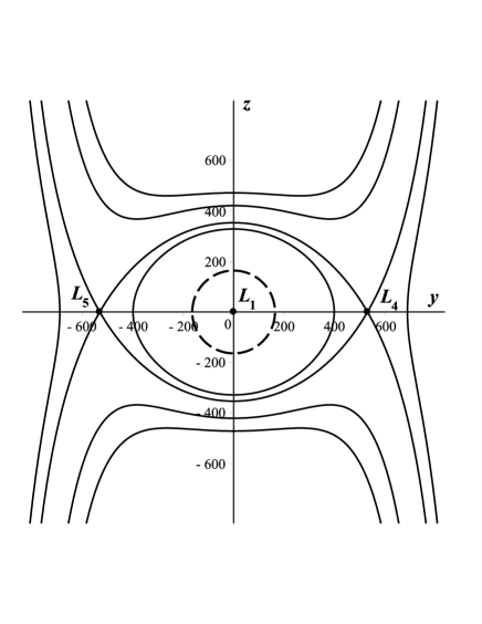
Figure 1: Zero-velocity surfaces with collinear $L_{1},L_{2},L_{3}$ and triangular, $L_{4},L_{5}$ libration points for EG NGC 4472 for Model 5 in the plane $x=0$. On the left is option 2 without a halo; on the right is option 1 with the halo. The dashed line marks the boundariesof the luminous part of the galaxy (left) and the galactic halo (right). Coordinates are given in kiloparsecs.

8. CONCLUSIONS

The spatial motion of a PGB in the gravitational field of a LIEG is considered on the basis of the new Model 5 for solving problems of celestial mechanics and astrophysics. According to Model 5, an EG with a halo (option 1) or without a halo (option 2) is a layered inhomogeneous elongated spheroid consisting of BM and DM. The choice of an elongated spheroid as a model for a triaxial EG is explained by the fact that its dynamic properties are very close to those of a triaxial ellipsoid. In this model, there is no interface between the BM and DM. Therefore, the determination of the conditions for matching the potentials is not con- sidered.

The so-called “astrophysical law” was taken as the BM profile; it is based on the Hubble surface brightness distribution law, which adequately models the density distribution in an EG. For the DM, an analogue of the NFW profile was taken.

An analogue of the Jacobi integral was found, the region of the possible motion of the PGB was determined, and the zero-velocity surfaces were constructed. The stationary solutions (libration points) were found to be stable in the sense of Lyapunov. Collinear libration points $L_{2}$ and $L_{3}$ found according to Models 3, 4, and 5 are conical singular points with a cone axis $OX$ and are unstable in the sense of Lyapunov in the first approximation. Triangular libration points $L_{4}$ and $L_{5}$ are singular points with a cone axis $OZ$ and are stable. The surface around the luminous part of the EG, within which the motions of the stars or the center of mass of the GC are Hill-stable, was determined.

The equilibrium and stability of the considered dynamical systems according to these two models will be studied by the author separately.

ACKNOWLEDGMENTS

The author is grateful to Prof. B.P. Kondrat’ev for valu- able advice and comments.

CONFLICT OF INTEREST

The author declares that he has no conflicts of interest.

REFERENCES

1.S. A. Gasanov, Astron. Rep. 56, 469 (2012).

2.S. A. Gasanov, Astron. Rep. 58, 167 (2014).

3.S. A. Gasanov, Astron. Rep. 59, 238 (2015).

4.S. A. Gasanov, Astron. Rep. 65, 723 (2021).

5.B. P. Kondrat’ev, Sov. Astron. 26, 279 (1982).

6.A. V. Zasov, A. S. Saburova, A. V. Khoperskov, and S.A. Khoperskov, Phys. Usp. 60, 3 (2017).

7.G. Bertin, R. P. Saglia, and M. Stiavelli, Astrophys. J. 384, 423 (1992).

8.M. Oguri, C. E. Rusu, and E. E. Falco, Mon. Not. R. Astron. Soc. 439, 2494 (2014).

9.G. de Vaucouleurs, A. de Vaucouleurs, H. Corwin, R.J. Buta, G. Paturel, and P. Fouque, Third Reference Catalouge of Bright Galaxies (Springer, New York, 1991), Vols. 2, 3.

10.G. N. Duboshin, Celestial Mechanics, Basic Problems and Methods (Nauka, Moscow, 1968) [in Russian].

11.H. Poincare, Lecons sur les hypotheses cosmogoniques (Lib. Sci. A. Hermann et fils, Paris, 1911).

12.B. P. Kondrat’ev, Potential Theory. New Methods and Problems with Solutions (Mir, Moscow, 2007) [in Rus- sian].

13.B. P. Kondrat’ev, Cand. Sci. (Phys. Math.) Disserta- tion (Mosc. Phys. Tech. Inst., Moscow, 1982).

14.E. Hubble, Astrophys. J. 71, 231 (1930).

15.J. F. Navarro, C. S. Frenk, and S. D. M. White, Astro- phys. J. 490, 493 (1997).

16.Yu. V. Batrakov, Byull. ITA 6, 524 (1957).

17.V. K. Abalakin, Byull. ITA 6, 543 (1957).

18.S. G. Zhuravlev, Sov. Astron. 18, 792 (1974).