Cooperative Distributed MPC via Decentralized Real-Time Optimization:
Implementation Results for Robot Formations

Abstract

Distributed model predictive control (DMPC) is a flexible and scalable feedback control method applicable to a wide range of systems. While the stability analysis of DMPC is quite well understood, there exist only limited implementation results for realistic applications involving distributed computation and networked communication. This article approaches formation control of mobile robots via a cooperative DMPC scheme. We discuss the implementation via decentralized optimization algorithms. To this end, we combine the alternating direction method of multipliers with decentralized sequential quadratic programming to solve the underlying optimal control problem in a decentralized fashion with nominal convergence guarantees. Our approach only requires coupled subsystems to communicate and does not rely on a central coordinator. Our experimental results showcase the efficacy of DMPC for formation control and they demonstrate the real-time feasibility of the considered algorithms.

[TUDO]organization=Institute for Energy Systems, Energy Efficiency and Energy Economics, TU Dortmund University,addressline=44227 Dortmund,country=Germany

[UStuttgart]organization=Institute of Engineering and Computational Mechanics, University of Stuttgart, addressline=70569 Stuttgart,country=Germany

1 Introduction

Model predictive control (MPC) is an advanced feedback design, which provides a structured framework for regulation, stabilization, and other control tasks. Motivated by the success of predictive control in applications, numerous distributed MPC (DMPC) schemes have been proposed for cyber-physical systems with applications ranging from energy systems (Venkat et al., 2008) to robot swarms (Van Parys and Pipeleers, 2017). Cooperative distributed control utilizes local sensing, local computation, and networked capabilities of subsystems to replace a centralized controller. Put differently, the subsystems cooperatively solve the control task, which improves scalability compared to a centralized approach (Müller and Allgöwer, 2017).

Robotic swarms are a prime application to study and showcase the intricacies of distributed control and to demonstrate the advantages of cooperative DMPC. On the one hand, this is motivated from a theoretical perspective since robotic swarms exhibit many challenges of distributed control—plant-model mismatch, issues of communication, high sampling frequency, as well as highly cooperative and scalable tasks with numerous possible constraints. Moreover, physical robotic cooperation is often rather intuitive, making it straight-forward to measure, to analyze, to depict, and to grasp the performance of different distributed schemes. On the other hand, progress in this area is highly relevant to engineering applications. Well-controlled swarms of land-based and aerial mobile robots are expected to revolutionize logistics, transportation, and security (Grau et al., 2017; Wen et al., 2018).

Figure 1: Control architectures and corresponding optimization architectures for MPC. This article discusses DMPC via decentralized optimization.

The present article considers formation control of mobile robots, which is one of the fundamental tasks in distributed robotics (Olfati-Saber et al., 2007; Bai et al., 2011). Specifically, formation control can serve as a building block for many relevant applications, such as cooperative transportation and manipulation (Ebel and Eberhard, 2022). Moreover, formation control has served as an example for the development and evaluation of DMPC. For instance, Yan and Bitmead (2003) present one of the early applications of MPC for the formation control of vehicles, although they focus on one-dimensional formations do not validate the scheme on hardware. Gu and Yang (2005) consider a centralized optimal control problem (OCP) for two-dimensional formations, but conducted no hardware experiments. In contrast, Kanjanawanishkul and Zell (2008) tested an MPC-based formation controller on real-world omnidirectional mobile robots where each robot runs its own controller. However, there is a centralized leader agent and the remaining robots merely follow the leader by using a conventional MPC controller to track the trajectory predicted by the leader, which does not fit today’s notion of cooperative DMPC where robots jointly solve an optimization problem. Yet, Kanjanawanishkul and Zell (2008) as well as Kuwata et al. (2007) seem to be among the first to deploy DMPC with distributed computation and communication on hardware. Since then, formation control has remained a popular benchmark problem accompanying the theoretical and numerical progress of DMPC. For instance, Ebel et al. (2017) compare sequential and cooperative DMPC methods for linear systems and analyze the performance of both schemes for a formation control task with hardware. Similarly, Ebel and Eberhard (2021) use formation control to compare a cooperative DMPC scheme to a distributed control method based on algebraic graph theory, confirming advantages of DMPC with respect to constraint handling also in hardware experiments. Recently, Burk et al. (2021a) tested the performance of an open-source DMPC framework with formation control, including real-world hardware but without distributed computation in the experiments. Novoth et al. (2021) study more complex scenarios including obstacle avoidance, but without the consideration of hardware experiments and distributed computation. Often in formation control, omnidirectional mobile robots are considered, whereas Rosenfelder et al. (2022) tailor a DMPC controller also to mobile robots with non-holonomic constraints.

From the systems and control point of view, one can distinguish different architectures ranging from centralized via distributed to decentralized schemes, cf. Figure 1 a). However, the notions for distributed and decentralized architectures differ slightly in control and optimization, cf. Figure 1 b). Specifically, in centralized feedback architectures, a single unit $\mathcal{C}$ controls all subsystems $\Sigma_{i}$. If $\mathcal{C}$ is an MPC controller, then a centralized OCP is solved via so-called centralized optimization algorithms. If the OCP is solved such that the computation is distributed onto subsystems that communicate both with one another and with a coordinator, then one speaks of a hierarchically distributed architecture. Finally, in distributed control, there exists a local controller $\mathcal{C}_{i}$ for each subsystem $\Sigma_{i}$ and these controllers communicate only with other controllers, but not with a central coordinator. To obtain such a distributed architecture, the OCP needs to be solved via decentralized algorithms which only require subsystem-to-subsystem communication. Finally, in decentralized control, each subsystem $\Sigma_{i}$ is controlled by a controller $\mathcal{C}_{i}$ and there is no communication between the controllers. This corresponds to separable OCPs which are solved by each subsystem individually without any communication. We refer to (Scattolini, 2009) for an overview of MPC architectures and to (Bertsekas and Tsitsiklis, 1989; Nedić et al., 2018) for the taxonomy of distributed and decentralized optimization. In order to tackle the robot formation control problem, this article focuses on cooperative DMPC, where the underlying centralized OCP is solved iteratively via decentralized optimization algorithms. That is, we implement a distributed controller through decentralized optimization.

In principle, the chosen approach of solving a centralized OCP via decentralized optimization can achieve a performance equivalent to a centralized MPC controller. In practice, the performance of DMPC is likely slightly worse than the one of centralized MPC, because the number of optimizer iterations per sampling interval is limited. There exists a range of decentralized optimization methods applicable to DMPC and we refer to (Stomberg et al., 2022a) for a recent overview for linear-quadratic problems. In particular the alternating direction method of multipliers (ADMM) shows promising performance in numerical studies (Conte et al., 2012; Rostami et al., 2017). ADMM is guaranteed to converge for convex problems (Boyd et al., 2011), but lacks convergence guarantees for general non-convex constraints arising from nonlinear dynamics or otherwise. A decentralized method with convergence guarantees also for non-convex problems is the recently proposed decentralized sequential quadratic programming (dSQP) method, which combines an SQP scheme with ADMM (Stomberg et al., 2022b) in a bi-level fashion.

The design, numerical implementation, and stability of cooperative DMPC are addressed in (Stewart et al., 2011; Giselsson and Rantzer, 2014; Conte et al., 2016; Köhler et al., 2019; Bestler and Graichen, 2019). Stewart et al. (2011) propose a tailored optimization method where each subsystem is equipped with the models of all subsystems such that the optimization method generates feasible iterates. Stability then follows from the design of terminal ingredients in the OCP. Giselsson and Rantzer (2014) and Köhler et al. (2019) guarantee stability through constraint tightening when applying dual decomposition to OCP designs with and without terminal ingredients, respectively. Bestler and Graichen (2019) develop a stopping criterion for ADMM to guarantee stability under the assumption that ADMM converges linearly for non-convex OCPs.

However, there exist only few experimental results to validate the developed DMPC schemes under real-world conditions. Therefore, we focus on the implementation, numerics, and experimental testing with real robot hardware. Van Parys and Pipeleers (2017) and Burk et al. (2021a) made notable contributions to the experimental validation of cooperative DMPC. The former tested an ADMM-based DMPC scheme on non-holonomic mobile robots with nonlinear dynamics. The DMPC algorithm was implemented on embedded computers onboard the robots such that there was one computing entity per robot. While the control performance was satisfactory, only a single ADMM iteration could be applied per control step due to the high computational complexity of the nonlinear program (NLP) each robot had to solve online. Even with infinitely many iterations, the application of ADMM to problems with non-convex constraint sets does not admit general convergence guarantees. Burk et al. (2021a) tested the open-source framework GRAMPC-D for the cooperative control of nonlinear unicycles running multiple ADMM iterations per control step. However, the test setup did not allow for true distributed execution as all control algorithms were implemented on a single computer.

This article focuses on the practical application of available DMPC methods and presents experimental results for ADMM- and dSQP-based DMPC schemes for a team of omnidirectional mobile robots. We use ADMM (Boyd et al., 2011) if the OCP transfers into a convex quadratic program (QP), and we use dSQP (Stomberg et al., 2022b) if a non-convex NLP is obtained. In both cases, only QPs are solved on a subsystem level, which allows to use the efficient active set method qpOASES tailored to MPC (Ferreau et al., 2014). Our decentralized and efficient implementation of ADMM- and dSQP-based DMPC allows to run multiple optimizer iterations per control step. We assign a single computer to each robot and thus we can test the algorithms in a distributed control setting.

The main contribution of this article is the practical evaluation of a decentralized optimization algorithm for DMPC. Specifically and to the best of the authors’ knowledge, the present paper appears to be the first to present experimental implementation results for cooperative distributed MPC with non-convexity in the underlying OCPs and with nominal convergence guarantees of the employed algorithm.

The paper is structured as follows. Section 2 introduces the DMPC scheme and the OCP. Section 3 presents ADMM and dSQP for solving the optimization problem. Section 4 gives an overview of implementational aspects with regard to the algorithms and experimental realization. Section 5 analyses the performance and execution time of the DMPC schemes and gives valuable insights for the future development of distributed optimization algorithms tailored to the needs of DMPC.

Notation: Given a matrix $A$ and an integer $j$, $[A]_{j}$ denotes the $j$th row of $A$. For an index set $\mathcal{A}$, $[A]_{\mathcal{A}}$ denotes the matrix consisting of rows $[A]_{j}$ for all $j\in\mathcal{A}$. Likewise, $[a]_{j}$ is the $j$th component of vector $a$ and $a_{\mathcal{A}}$ is the vector of components $[a]_{j}$ for all $j\in\mathcal{A}$. The concatenation of vectors $x$ and $y$ into a column vector is $\text{col}(x,y)$. Likewise, $\text{col}(x_{i})_{i\in\mathcal{S}}$ denotes the concatenation of vectors $x_{i}$ for all $i\in\mathcal{S}$. The $\varepsilon$-neighborhood around a point $x\in\mathbb{R}^{n}$ is denoted by $\mathcal{B}_{\varepsilon}(x)$, i.e., ${\mathcal{B}_{\varepsilon}(x)\doteq\{y\in\mathbb{R}^{n}\ |\ \|y-x\|\leq\varepsilon\}}$, where $\|\cdot\|$ is some norm on $\mathbb{R}^{n}$. Further, $A=[A_{ij}]$ is the block matrix with entries $A_{ij}$ at block position $(i,j)$. $I$ is the identity matrix. The set $\mathbb{I}_{[0,N]}$ denotes the integers in the range $[0,N]$. The time is denoted by $t$.

2 Problem Statement

Let $\mathcal{S}=\{1,\dots,S\}$ be a set of mobile robots. The state and input of robot $i\in\mathcal{S}$ are denoted as $x_{i}\in\mathbb{R}^{n_{x,i}}$ and $u_{i}\in\mathbb{R}^{n_{u,i}}$. In this article, the state $x_{i}$ represents the position of robot $i$ with respect to a fixed coordinate system, and the input $u_{i}$ represents the desired translational velocity of the robot body. The centralized position and velocity of all robots are $x\doteq\text{col}(x_{i})_{i\in\mathcal{S}}\in\mathbb{R}^{n_{x}}$ and $u\doteq\text{col}(u_{i})_{i\in\mathcal{S}}\in\mathbb{R}^{n_{u}}$.

2.1 DMPC of Mobile Robots

We consider the task where the centralized position $x$ tracks a desired formation $\bar{x}(t)\doteq\text{col}(\bar{x}_{i}(t))_{i\in\mathcal{S}}$. Figure 2 shows one of the custom mobile robots we use for the experimental validation of our approach (Ebel and Eberhard, 2022). The omnidirectional robots move in the $X$-$Y$-plane and they can accelerate into any direction at any time, independent from their orientation. The (approximate) dynamics of each robot used for prediction in the controller are given by ${f_{i}^{\mathrm{d}}(x_{i},u_{i})=x_{i}+\Delta t\,u_{i}}$, where $\Delta t$ denotes the control sampling interval and where ${n_{x,i}=n_{u,i}=2}$.

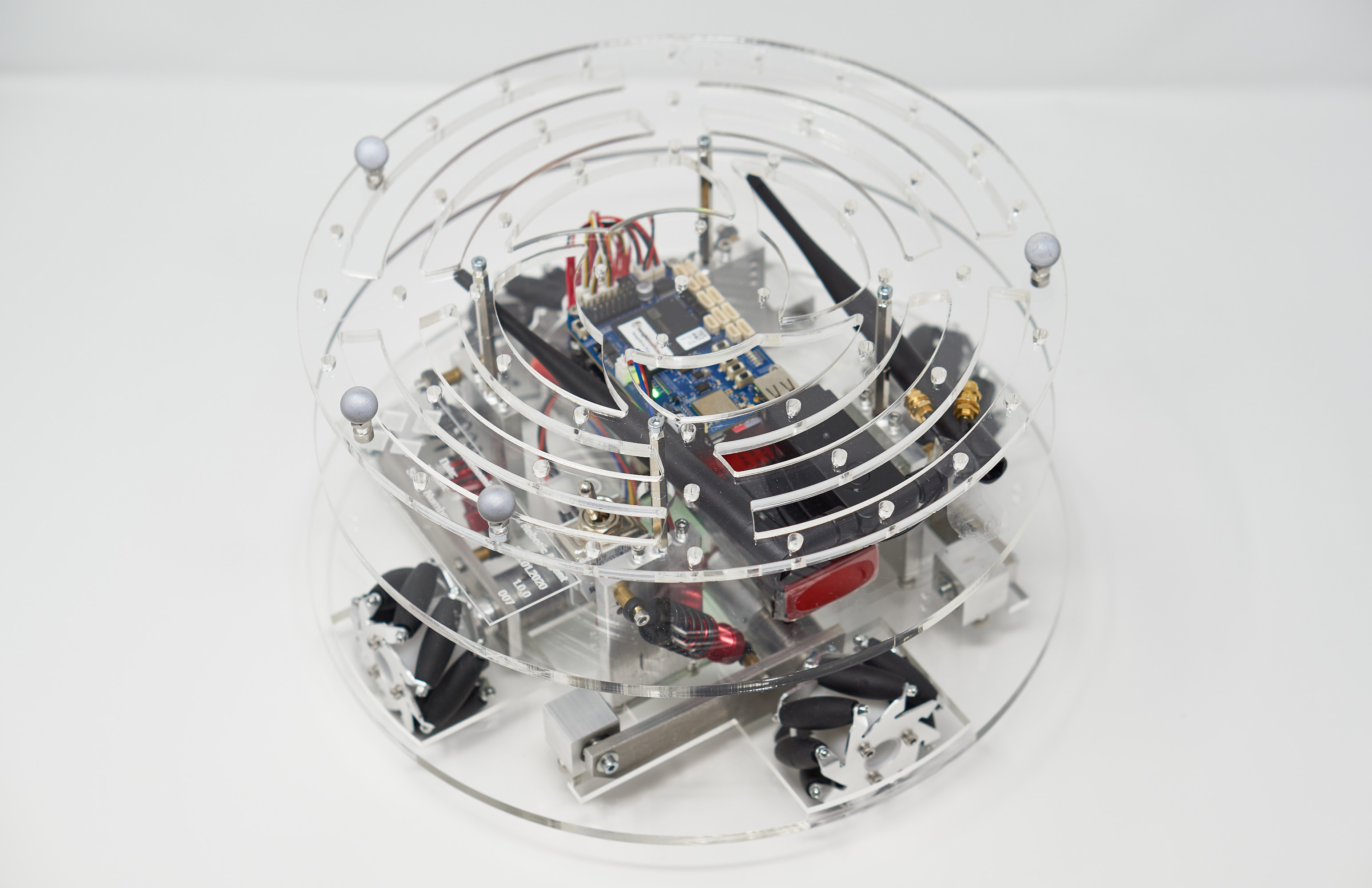
Figure 2: Omnidirectional mobile robot for distributed robotics experiments.

2.2 OCP Formulation

To design the DMPC scheme, we first formulate a centralized OCP

$$\min_{\boldsymbol{x},\boldsymbol{u}} \sum_{i\in\mathcal{S}}\sum_{k=0}^{N-1}\ell_{i}(x^{k},u_{i}^{k})+V_{\text{f},i}(x^{N})$$ (1a)

subject $$\text{ to for all }i\in\mathcal{S}$$

$$x_{i}^{k+1} =f_{i}^{\mathrm{d}}(x_{i}^{k},u_{i}^{k}), \forall k\in\mathbb{I}_{[0,N-1]},$$ (1b)

$$(x_{i}^{0},u_{i}^{0}) =(x_{i}(t),u_{i}(t)),$$ (1c)

$$x_{i}^{k} \in\mathbb{X}_{i} \forall k\in\mathbb{I}_{[0,N]},$$ (1d)

$$u_{i}^{k} \in\mathbb{U}_{i} \forall k\in\mathbb{I}_{[0,N-1]},$$ (1e)

$$(x_{i}^{k},x_{j}^{k}) \in\mathbb{X}_{ij},\hskip 13.942pt\forall j\in\mathcal{S}, \forall k\in\mathbb{I}_{[0,N]}.$$ (1f)

The decision variables $\boldsymbol{x}\doteq\text{col}(x^{k})_{k\in\mathbb{I}_{[0,N]}}$ and $\boldsymbol{u}\doteq\text{col}(u^{k})_{k\in\mathbb{I}_{[0,N-1]}}$ are the predicted trajectories over the horizon $N$. OCP (1) couples the robots via the stage cost ${\ell_{i}:\mathbb{R}^{n_{x,1}}\times\dots\times\mathbb{R}^{n_{x,S}}\times\mathbb{R}^{n_{u,i}}\rightarrow\mathbb{R}}$,

$$\ell_{i}(x,u_{i})\doteq\sum_{j\in\mathcal{S}}\frac{1}{2}(x_{i}-\bar{x}_{i})^{\top}Q_{ij}(x_{j}-\bar{x}_{j})+\frac{1}{2}(u_{i}-\bar{u}_{i})^{\top}R_{ii}(u_{i}-\bar{u}_{i}),$$

via the terminal penalty $V_{\text{f},i}:\mathbb{R}^{n_{x,1}}\times\dots\times\mathbb{R}^{n_{x,S}}\rightarrow\mathbb{R}$,

$$V_{\text{f},i}(x)\doteq\frac{1}{2}\sum_{j\in\mathcal{S}}(x_{i}-\bar{x}_{i})^{\top}P_{ij}(x_{j}-\bar{x}_{j}),$$

where $Q_{ij}\in\mathbb{R}^{n_{x,i}\times n_{x,j}}$, $R_{ii}\in\mathbb{R}^{n_{u,i}\times n_{u,i}}$, and $P_{ij}\in\mathbb{R}^{n_{x,i}\times n_{x,j}}$ are weight matrices, and via the constraints (1f), where $\mathbb{X}_{ij}\subseteq\mathbb{R}^{n_{x,i}}\times\mathbb{R}^{n_{x,j}}$. The sets $\mathbb{X}_{i}\subseteq\mathbb{R}^{n_{x,i}}$ and $\mathbb{U}_{i}\subseteq\mathbb{R}^{n_{u,i}}$ constrain the states and inputs of subsystem $i$, respectively. The coupling in OCP (1) describes the cooperation between the robots to achieve the control task.

We only consider state coupling in OCP (1) and refer to (Stomberg et al., 2022a) for an extension to input coupling. The coupling structure of OCP (1) can be represented as a graph and we define for each robot $i$ sets of in- and out-neighbors

$$\mathcal{N}_{i}^{\text{in}} \doteq\left\{j\in\mathcal{S}\backslash\{i\}\ |\ Q_{ij}\neq 0\cup P_{ij}\neq 0\cup\mathbb{X}_{ij}\neq\mathbb{R}^{n_{x,i}}\times\mathbb{R}^{n_{x,j}}\right\},$$

$$\mathcal{N}_{i}^{\text{out}} \doteq\left\{j\in\mathcal{S}\ |\ i\in\mathcal{N}_{j}^{\text{in}}\right\}.$$

We make the following two assumptions on the communication between subsystems and on OCP (1).

Assumption 1 (Communication graph)

We assume that the communication graph is equivalent to the coupling graph, i.e., each subsystem $i$ communicates bi-directionally with all its neighbors $\mathcal{N}_{i}\doteq\mathcal{N}_{i}^{\text{in}}\cup\mathcal{N}_{i}^{\text{out}}$ to solve OCP (1) cooperatively. We further assume that no messages are lost between subsystems.

Assumption 2 (OCP (1) requirements)

m

1. The centralized weight matrices $Q\doteq[Q_{ij}]\in\mathbb{R}^{n_{x}\times n_{x}}$,
   $R\doteq[R_{ij}]\in\mathbb{R}^{n_{u}\times n_{u}}$, and $P\doteq[P_{ij}]\in\mathbb{R}^{n_{x}\times n_{x}}$ are symmetric positive definite.

2. The sets $\mathbb{X}_{i}$, $\mathbb{U}_{i}$, and $\mathbb{X}_{ij}$ are closed for all $i,j\in\mathcal{S}$. $\square$

Most approaches in the literature guarantee closed-loop stability based on Assumption 2 combined with additional assumptions on the compactness of the constraint sets $\mathbb{X}_{i}$ and $\mathbb{U}_{i}$, the design of terminal constraints and terminal penalties, and initial feasibility of the OCP. Here, we omit the design of specific terminal ingredients and instead focus on the numerical implementation and the experimental validation. Instead we refer to (Conte et al., 2016) and (Darivianakis et al., 2019) for the design of terminal ingredients in DMPC. Moreover, we allow for a non-convex set $\mathbb{X}_{i}$ as this enables guaranteeing collision avoidance via encoding minimum-distance requirements between robots in tailored constraints.

Algorithm 1 summarizes the considered DMPC scheme. Per MPC step, each robot first measures its current position $x_{i}(t)$. Then, the robots solve OCP (1) cooperatively using a decentralized optimization method. The second element $u_{i}^{1}$ of the optimal open-loop input trajectory $\boldsymbol{u}_{i}^{\star}$ is then chosen as input $u_{i}(t+\Delta t)$ in the next MPC step.

Remark 1 (Compensation of computational delay)

The The careful reader will notice that (1c) imposes an initial condition on the input. This choice allows to compensate the computational delay of Steps 3 and 4 of Algorithm 1. Solving the OCP in decentralized fashion can take a substantial fraction of the samping interval due to the iterative nature of decentralized optimization methods and due to communication latencies between robots. Applying $u_{i}^{1}$ in the next MPC step instead of applying $u_{i}^{0}$ in the current MPC step compensates for the inevitable computational delay (Findeisen, 2006). This approach therefore requires the combined execution time for Steps 3–5 of Algorithm 1 to be less than $\Delta t$. $\square$

Algorithm 1 Cooperative distributed MPC

1:Initialization: $u_{i}(0),\bar{x}_{i}$ for all $i\in\mathcal{S}$

2:while $t<t_{\text{end}}$ for all $i\in\mathcal{S}$ do

3:     Measure $x_{i}(t)$ for all $i\in\mathcal{S}$

4:     Solve OCP (1) via decentralized optimization

5:     Extract $u_{i}^{1}$ from $\boldsymbol{u}_{i}^{\star}$

6:     $u_{i}(t+\Delta t)=u_{i}^{1}$

7:     $t=t+\Delta t$

8:end while

2.3 Reformulation as Partially Separable Problem

To obtain a DMPC scheme, we solve OCP (1) online via iterative decentralized optimization methods. To this end, we introduce state copies $w_{ji}^{k}=x_{j}^{k}$ for all $j\in\mathcal{N}_{i}^{\text{in}}$ and for all $i\in\mathcal{S}$. The trajectory copies $\boldsymbol{w}_{i}\doteq\text{col}(w_{i}^{k})_{k\in\mathbb{I}_{[0,N]}}$ with $w_{i}^{k}\doteq\text{col}(w_{ji}^{k})_{j\in\mathcal{N}_{i}^{\text{in}}}$ are additional decision variables of subsystem $i$ and $w_{i}^{k}$ replaces $x_{j}^{k}$ in (1a), (1b), and (1f) for all $j\in\mathcal{N}_{i}^{\text{in}}$. We reformulate OCP (1) with $z_{i}\doteq\text{col}(\boldsymbol{x}_{i},\boldsymbol{u}_{i},\boldsymbol{w}_{i})\in\mathbb{R}^{n_{i}}$ as the partially separable NLP

$$\min_{z_{i}\in\mathbb{R}^{n_{i}},i\in\mathcal{S}} \sum_{i\in\mathcal{S}}f_{i}(z_{i})$$ (2a)

subject to

$$g_{i}(z_{i}) =0\quad\;|\;\nu_{i},\quad\forall i\in\mathcal{S},$$ (2b)

$$h_{i}(z_{i}) \leq 0\quad\;|\;\mu_{i},\quad\forall i\in\mathcal{S},$$ (2c)

$$\sum_{i\in\mathcal{S}}E_{i}z_{i} =0\quad\;|\;\lambda,$$ (2d)

where $f_{i}:\mathbb{R}^{n_{i}}\rightarrow\mathbb{R}$, $g_{i}:\mathbb{R}^{n_{i}}\rightarrow\mathbb{R}^{n_{g,i}}$, and $h_{i}:\mathbb{R}^{n_{i}}\rightarrow\mathbb{R}^{n_{h,i}}$ are twice continuously differentiable. The notation in (2) highlights that $\nu_{i}$, $\mu_{i}$, and $\lambda$ are the Lagrange multipliers to (2b), (2c), and (2d). The objective ${f_{i}(z_{i})\doteq 1/2\,z_{i}^{\top}H_{i}z_{i}+g_{i}^{\top}z_{i}}$ of subsystem $i$ represents (1a) and the matrices $H_{i}$ are composed of the weight matrices $Q_{ij},R_{ii}$, and $P_{ij}$. The equality constraint (2b) includes the system dynamics (1b) and the initial condition (1c). Depending on the type of constraint, (1d)–(1f) are part of (2b) or (2c). The constraint (2d) couples states and copies, see (Stomberg et al., 2022a, Example 1).

Remark 2 (Soft-constrained optimal control problem)

We Since we omit the design of tailored terminal penalties and terminal constraints, OCP (1) is not guaranteed to be recursively feasible in the presence of state constraints. Therefore, we introduce a scalar slack variable $s_{i}\geq 0$ as an additional decision variable for each robot, cf. (Maciejowski, 2002, Eq. 3.91). We then replace any hard inequality constraint $[h_{i}(z_{i})]_{p}$ in (2c) corresponding to a state constraint by the soft inequality constraint $[h_{i}(z_{i})]_{p}\leq s_{i}$. The slack $s_{i}$ is penalized by adding $cs_{i}^{2}$ with $c\gg 0$ to (2a). Note that the soft-constrained problem obtained this way is always feasible. $\square$

3 Decentralized Optimization

The key concept to implement Algorithm 1 as a distributed controller lies in the solution of the centralized OCP using decentralized optimization methods. That is, we use methods that only require robots that are neighbors in the underlying graph to communicate with each other for solving the OCP. Specifically, this section discusses an ADMM variant and dSQP.

3.1 Essentials of ADMM

To apply ADMM, we introduce the auxiliary decision variable $\bar{z}_{i}\in\mathbb{R}^{n_{i}}$ for each subsystem and rewrite (2) as

$$\min_{z_{i}\in\mathbb{Z}_{i},\bar{z}_{i}\in\mathbb{R}^{n_{i}},i\in\mathcal{S}}\quad \sum_{i\in\mathcal{S}}f_{i}(z_{i})$$ (3a)

subject to

$$z_{i}-\bar{z}_{i} =0\quad\;|\;\gamma_{i},\quad\forall i\in\mathcal{S},$$ (3b)

$$\sum_{i\in\mathcal{S}}E_{i}\bar{z}_{i} =0,$$ (3c)

where $\gamma_{i}\in\mathbb{R}^{n_{i}}$ are Lagrange multipliers associated to (3b), and where $\mathbb{Z}_{i}\doteq\{z_{i}\in\mathbb{R}^{n_{i}}\ |\ g_{i}(z_{i})=0,h_{i}(z_{i})\leq 0\}$. Let $z\doteq\text{col}(z_{i})_{i\in\mathcal{S}}$, $\bar{z}\doteq\text{col}(\bar{z}_{i})_{i\in\mathcal{S}}$, and $\gamma\doteq\text{col}(\gamma_{i})_{i\in\mathcal{S}}$ denote the centralized variables in (3). The augmented Lagrangian of (3) is given by

$$L_{\rho}(z,\bar{z},\gamma) =\sum_{i\in\mathcal{S}}L_{\rho,i}(z_{i},\bar{z}_{i},\gamma_{i})$$

$$=\sum_{i\in\mathcal{S}}f_{i}(z_{i})+\gamma_{i}^{\top}(z_{i}-\bar{z}_{i})+\frac{\rho}{2}\|z_{i}-\bar{z}_{i}\|_{2}^{2},$$

where $\rho\in\mathbb{R}^{+}$ is called penalty parameter. The ADMM iterations read

$$z_{i}^{l+1} =\operatorname*{argmin}_{z_{i}\in\mathbb{Z}_{i}}L_{\rho,i}(z_{i},\bar{z}_{i}^{l},\gamma_{i}^{l}),$$ (4a)

$$\bar{z}^{l+1} =\operatorname*{argmin}_{\bar{z}\in\mathbb{E}}L_{\rho}(z^{l+1},\bar{z},\gamma^{l}),$$ (4b)

$$\gamma_{i}^{l+1} =\gamma_{i}^{l}+\rho(z_{i}^{l+1}-\bar{z}_{i}^{l+1}),$$ (4c)

where $\mathbb{E}\doteq\{\bar{z}\in\mathbb{R}^{n}\,|\,E\bar{z}\doteq 0\},$ and $E\doteq[E_{1},\dots,E_{S}].$ Each subsystem computes the updates (4a) and (4c) individually. The update (4b) is equivalent to an efficient averaging step if the Lagrange multiplier initialization $\gamma^{0}$ satisfies

$$(I-E^{\top}(EE^{\top})^{-1}E)\gamma^{0}=0.$$ (5)

Such an initialization may be obtained by choosing $\gamma^{0}=0$, or by warm-starting with a solution obtained from a previous execution of ADMM. The averaging procedure is given in Steps 4–7 of Algorithm 2. First, in Step 4, each subsystem sends the updated copy values obtained in Step 3 to its in-neighbors and receives the updated copies corresponding to its own trajectory from its out-neighbors. In Step 5, each subsystem averages all decision variables corresponding to its state trajectory. Then, in Step 6, each subsystem shares the averaged values with all out-neighbors and receives the averaged values from all in-neighbors. Finally, in Step 7, each subsystem forms $\bar{z}_{i}^{l+1}$ from the mean values. Upon ADMM convergence, (3b) holds and the subsystems have reached consensus.

ADMM has successfully been used both for DMPC of linear systems (Rostami et al., 2017) and for nonlinear DMPC (Bestler and Graichen, 2019). If OCP (1) is an NLP, then each robot solves an NLP in Step 3 of ADMM. This is computationally expensive and using general-purpose NLP solvers such as IPOPT (Wächter and Biegler, 2006)–especially if deployed on embedded hardware—may limit the number of ADMM iterations per MPC step (Van Parys and Pipeleers, 2017). If instead OCP (1) is a QP, then each robot only solves a QP in each ADMM iteration, which is computationally much less demanding.

ADMM is guaranteed to converge for convex problems (Boyd et al., 2011; He and Yuan, 2012). While ADMM is guaranteed to converge also for some non-convex problems (Wang et al., 2019), there exist no generally applicable convergence results if OCP (1) is non-convex as is the case in distributed nonlinear MPC. We therefore use Algorithm 2 if OCP (1), or respectively its reformulation (2), is a convex QP.

Algorithm 2 ADMM for OCP (2) (Boyd et al., 2011)

1:Initialization: $l=0$, $\bar{z}_{i}^{0},\gamma_{i}^{0}$ satisfying (5) for all $i\in\mathcal{S}$, $l_{\mathrm{max}}$

2:while $l<l_{\mathrm{max}}$ for all $i\in\mathcal{S}$ do

3:     Solve subsystem program $z_{i}^{l+1}=\displaystyle\operatorname*{argmin}_{z_{i}\in\mathbb{Z}_{i}}L_{\rho,i}(z_{i},\bar{z}_{i}^{l},\gamma_{i}^{l})$

4:     Receive copies $\boldsymbol{w}^{l+1}_{ij}$ from all ${j\in\mathcal{N}_{i}^{\text{out}}}$

5:     Average received copies with original trajectories

$$\bar{\boldsymbol{x}}^{l+1}_{i}=\frac{1}{\lvert\mathcal{N}_{i}^{\text{out}}\rvert+1}\left(\boldsymbol{x}_{i}^{l+1}+\sum_{j\in\mathcal{N}_{i}^{\text{out}}}\boldsymbol{w}^{l+1}_{ij}\right)$$

6:     Send average $\bar{\boldsymbol{x}}^{l+1}_{i}$ to all $j\in\mathcal{N}_{i}^{\text{out}}$

7:     Form $\bar{z}_{i}^{l+1}=\text{col}(\bar{\boldsymbol{x}}^{l+1}_{i},\bar{\boldsymbol{u}}^{l+1}_{i},\bar{\boldsymbol{w}}^{l+1}_{i}),\,\bar{\boldsymbol{w}}^{l+1}_{i}=\text{col}(\bar{\boldsymbol{x}}^{l+1}_{j})_{j\in\mathcal{N}_{i}^{\text{in}}}$

8:     Update dual variable $\gamma_{i}^{l+1}=\gamma_{i}^{l}+\rho(z_{i}^{l+1}-\bar{z}_{i}^{l+1})$

9:     $l=l+1$

10:end while

11:return $z_{i}^{l}$

3.2 The Decentralized SQP Method for Nonlinear DMPC

To solve non-convex OCPs, we consider the dSQP algorithm proposed by (Stomberg et al., 2022b). Similar to (Engelmann et al., 2020), the method admits a bi-level structure, i.e., we index outer SQP iterations by $q$ and inner ADMM iterations by $l$. Let $\nu\doteq\text{col}(\nu_{i})_{i\in\mathcal{S}}$ and $\mu\doteq\text{col}(\mu_{i})_{i\in\mathcal{S}}$ denote the centralized dual variables of problem (2). Given a primal-dual iterate $(z^{q},\nu^{q},\mu^{q},\lambda^{q})$, we approximate (2) by

$$\min_{\Delta z_{i}\in\mathbb{R}^{n_{i}},i\in\mathcal{S}}\;\sum_{i\in\mathcal{S}}\frac{1}{2}\Delta z_{i}^{\top}H_{i}^{q}\Delta z_{i} +\nabla f_{i}(z_{i}^{q})^{\top}\Delta z_{i}$$ (6a)

subject to

$$g_{i}(z_{i}^{q})+\nabla g_{i}(z_{i}^{q})^{\top}\Delta z_{i} =0\quad\;|\;\nu_{i}^{\text{QP}},\quad\forall i\in\mathcal{S},$$ (6b)

$$h_{i}(z_{i}^{q})+\nabla h_{i}(z_{i}^{q})^{\top}\Delta z_{i} \leq 0\quad\;|\;\mu_{i}^{\text{QP}},\quad\forall i\in\mathcal{S},$$ (6c)

$$\sum_{i\in\mathcal{S}}E_{i}(z_{i}^{q}+\Delta z_{i}) =0\quad\;|\;\lambda^{\text{QP}},$$ (6d)

where the matrix $H_{i}^{q}\approx\nabla_{z_{i}z_{i}}^{2}L_{i}^{q}\doteq\nabla_{z_{i}z_{i}}^{2}L_{i}(z_{i}^{q},\nu_{i}^{q},\mu_{i}^{q},\lambda^{q})$ is positive definite, and where the Lagrangian function of subsystem $i$ is given by ${L_{i}(\cdot)=f_{i}(z_{i})+\nu_{i}^{\top}g_{i}(z_{i})+\mu_{i}^{\top}h_{i}(z_{i})+\lambda^{\top}E_{i}z_{i}}.$ The convex quadratic approximation (6) is solved in decentralized fashion via ADMM to obtain the SQP steps ${\Delta z_{i}=\text{col}(\Delta\boldsymbol{x}_{i},\Delta\boldsymbol{u}_{i},\Delta\boldsymbol{w}_{i})}$, ${\Delta\nu_{i}\doteq\nu_{i}^{\text{QP}}-\nu_{i}^{q}}$, $\Delta\mu_{i}\doteq\mu_{i}^{\text{QP}}-\mu_{i}^{q}$, and $\Delta\lambda\doteq\lambda^{\text{QP}}-\lambda^{q}$.

Algorithm 3 summarizes the dSQP iterations. For the sake of compact notation, we collect the subsystem constraint sets of QP (6) in

$$\mathbb{S}_{i}^{q}\doteq\left\{\Delta z_{i}\in\mathbb{R}^{n_{i}}\,\left|\,\begin{aligned} g_{i}(z_{i}^{q})+\nabla g_{i}(z_{i}^{q})^{\top}\Delta z_{i}&=0\\ h_{i}(z_{i}^{q})+\nabla h_{i}(z_{i}^{q})^{\top}\Delta z_{i}&\leq 0\end{aligned}\right.\right\}$$

and the augmented Lagrangian function of subsystem $i$ is

$$L_{\rho,i}^{QP,q}=\frac{1}{2}\Delta z_{i}^{\top}H_{i}^{q}\Delta z_{i}+\nabla f_{i}(z_{i}^{q})^{\top}\Delta z_{i}+\gamma_{i}^{\top}(\Delta z_{i}-\Delta\bar{z}_{i})+\frac{\rho}{2}\|\Delta z_{i}-\Delta\bar{z}_{i}\|_{2}^{2}.$$

Remark 3 (Local dSQP convergence)

We terminate ADMM after $l_{\mathrm{max}}$ iterations per outer iteration in Step 5 of Algorithm 3. This is due to practical reasons and limits the execution time of dSQP in each MPC step. However, one could also terminate ADMM in Step 5 of Algorithm 3 dynamically to obtain local convergence guarantees for dSQP. To obtain the convergence result, we define ${d_{i}\doteq\text{col}(\Delta z_{i},\Delta\nu_{i},\Delta\mu_{i})}$, $d=(\text{col}(d_{i})_{i\in\mathcal{S}},\Delta\lambda)$, and ${p\doteq\text{col}(z,\nu,\mu,\lambda)}$. Let ${p^{\star}\doteq\text{col}(z^{\star},\nu^{\star},\mu^{\star},\lambda^{\star})}$ be a Karush-Kuhn-Tucker (KKT) point of (2). We denote the set of active inequality constraints at $z_{i}^{\star}$ by $\mathcal{A}_{i}\doteq\{j\in\{1,\dots,n_{h,i}\}\ |\ [h_{i}(x_{i}^{\star})]_{j}=0\}$. The stopping criterion reads

$$\|\tilde{F}^{q}+\nabla\tilde{F}^{q}d\|\leq\eta^{q}\|\tilde{F}^{q}\|,$$ (7)

where

$$\tilde{F}\doteq\begin{bmatrix}\nabla_{z_{1}}L_{1}(z_{1},\nu_{1},\mu_{1},\lambda)\\ g_{1}(z_{1})\vspace*{-0.1cm}\\ \vdots\vspace*{-0.1cm}\\ \nabla_{z_{S}}L_{S}(z_{S},\nu_{S},\mu_{S},\lambda)\\ g_{S}(z_{S})\\ \sum_{i\in\mathcal{S}}E_{i}z_{i}\end{bmatrix},\nabla\tilde{F}=\begin{bmatrix}\nabla\tilde{F}_{1}&\dots&0&\bar{E}_{1}^{\top}\vspace*{-0.1cm}\\ \vdots&\ddots&\vdots&\vdots\\ 0&\dots&\nabla\tilde{F}_{S}&\bar{E}_{S}^{\top}\\ \tilde{E}_{1}&\dots&\tilde{E}_{S}&0\end{bmatrix},$$

$$\nabla\tilde{F}_{i}\doteq\begin{bmatrix}\nabla_{z_{i}z_{i}}^{2}L_{i}&\nabla g_{i}(z_{i})&\nabla h_{i}(z_{i})\\ \nabla g_{i}(z_{i})^{\top}&0&0\\ \end{bmatrix},$$

with $\tilde{E}_{i}\doteq\begin{bmatrix}E_{i}&0&0\end{bmatrix}$, $\bar{E}_{i}\doteq\begin{bmatrix}E_{i}&0\end{bmatrix}$, and $\eta^{q}\geq 0$. If this stopping criterion is employed, then dSQP is guaranteed to converge locally as described in Theorem 1 below, which appeared as Theorem 2 in (Stomberg et al., 2022b). $\square$

Theorem 1 (dSQP convergence (Stomberg et al., 2022b))

Let $p^{\star}$ be a KKT point of (2) which, for all $i\in\mathcal{S}$, satisfies

1. $h_{i}(z_{i}^{\star})+\mu_{i}^{\star}\neq 0$ (strict complementarity),

2. $\Delta z_{i}^{\top}\nabla_{z_{i}z_{i}}^{2}L_{i}(z_{i}^{\star},\nu_{i}^{\star},\mu_{i}^{\star},\lambda^{\star})\Delta z_{i}>0$ for all $\Delta z_{i}\neq 0$ with $\nabla g_{i}(x_{i}^{\star})^{\top}\Delta z_{i}=0$.

Furthermore, suppose the matrix

$$\begin{bmatrix}\nabla_{z_{1}}g_{1}(z_{1}^{\star})^{\top}&&\vspace*{-0.2cm}\\ &\ddots&\vspace*{-0.2cm}\\ &&\nabla_{z_{S}}g_{S}(z_{S}^{\star})^{\top}\\ \nabla_{z_{1}}[h_{1}(z_{1}^{\star})]_{\mathcal{A}_{1}}^{\top}&&\vspace*{-0.2cm}\\ &\ddots&\vspace*{-0.2cm}\\ &&\nabla_{z_{S}}[h_{S}(z_{S}^{\star})]_{\mathcal{A}_{S}}^{\top}\\ E_{1}&\dots&E_{S}\end{bmatrix}$$

has full row rank, i.e., $z^{\star}$ satisfies the linear independence constraint qualification. Furthermore, suppose the Hessian approximation ${H_{i}^{q}=\nabla_{z_{i}z_{i}}^{2}L_{i}^{q}}$ is used and that ADMM is terminated in Step 5 of Algorithm 3 dynamically based on (7). Then, there exist $\varepsilon>0$ and $\eta>0$ such that for all $p^{0}\in\mathcal{B}_{\varepsilon}(p^{\star})$ the following holds:

1. If $\eta^{q}\leq\eta$, then the sequence $\{p^{q}\}$ generated by Algorithm 3 converges to $p^{\star}$ and the convergence rate is q-linear in the outer iterations.

2. If $\eta^{q}\rightarrow 0$, then the convergence rate is q-superlinear in the outer iterations.

3. If $\eta^{q}=O(\|\tilde{F}^{q}\|)$ and if ${\nabla_{z_{i}z_{i}}^{2}f_{i},\nabla_{z_{i}z_{i}}^{2}[g_{i}]_{j},j\in\{1,\dots,n_{g,i}\}}$, and ${\nabla_{z_{i}z_{i}}^{2}[h_{i}]_{j},j\in\{1,\dots,n_{h,i}\}}$ are Lipschitz continuous inside $\mathcal{B}_{\varepsilon}$, then the convergence rate is q-quadratic in the outer iterations. $\square$

Remark 4 (Hessian approximation)

There exist two common choices for $H_{i}^{q}$. The first option is to set ${H_{i}^{q}=\nabla_{z_{i}z_{i}}^{2}L_{i}^{q}}$, and to regularize if needed. For the regularization, we follow a heuristic by changing the sign of negative eigenvalues (Engelmann et al., 2021). That is, we first compute an eigenvalue decomposition $\nabla_{z_{i}z_{i}}^{2}L_{i}^{q}=V_{i}\Lambda_{i}V_{i}^{\top}$. Then, we set $H_{i}^{q}=V_{i}\tilde{\Lambda}_{i}V_{i}^{\top}$, where for all $j\in\{1,\dots,n_{i}\}$

$$\tilde{\Lambda}_{i,jj}\doteq\left\{\begin{array}[]{ll}\varepsilon,&\text{if }\Lambda_{i,jj}\in[-\varepsilon,\varepsilon],\\ |\Lambda_{jj}|,&\text{else},\end{array}\right.$$

and $\varepsilon=10^{-4}$. The second option is the Gauss-Newton approximation $H_{i}^{q}=\nabla^{2}_{z_{i}z_{i}}f_{i}(z_{i})$ (Bock, 1983). In this case, $H_{i}^{q}$ is constant, strongly convex, and can be evaluated offline, because the objectives $f_{i}(\cdot)$ are strongly convex quadratic functions. $\square$

Algorithm 3 dSQP for OCP (2) (Stomberg et al., 2022b)

1:Initialization: $q=0,z_{i}^{0},\nu_{i}^{0},\mu_{i}^{0},\gamma_{i}^{0}$ satisfying (5) for all $i\in\mathcal{S},q_{\mathrm{max}},l_{\mathrm{max}}$

2:while $q<q_{\mathrm{max}}$ for all $i\in\mathcal{S}$ do

3:     Compute $\nabla f_{i}(z_{i}^{q}),\nabla g_{i}(z_{i}^{q}),\nabla h_{i}(z_{i}^{q}),H_{i}^{q}$ locally

4:     ADMM initialization $l=0,\Delta\bar{z}_{i}^{0}=0$

5:     while $l<l_{\mathrm{max}}$ do

6:         Solve QP $\Delta z_{i}^{l+1}=\displaystyle\operatorname*{argmin}_{\Delta z_{i}\in\mathbb{S}_{i}}L_{\rho,i}^{QP,q}(\Delta z_{i},\Delta\bar{z}_{i}^{l},\gamma_{i}^{l})$

7:         Receive copies $\Delta\boldsymbol{w}^{l+1}_{ij}$ from all ${j\in\mathcal{N}_{i}^{\text{out}}}$

8:         Average received copies with original trajectories

$$\Delta\bar{\boldsymbol{x}}^{l+1}_{i}=\frac{1}{\lvert\mathcal{N}_{i}^{\text{out}}\rvert+1}\left(\Delta\boldsymbol{x}_{i}^{l+1}+\sum_{j\in\mathcal{N}_{i}^{\text{out}}}\Delta\boldsymbol{w}^{l+1}_{ij}\right)$$

9:         Send average $\Delta\bar{\boldsymbol{x}}^{l+1}_{i}$ to all $j\in\mathcal{N}_{i}^{\text{out}}$

10:         $\Delta\bar{z}_{i}^{l+1}=\text{col}(\Delta\bar{\boldsymbol{x}}^{l+1}_{i},\Delta\bar{\boldsymbol{u}}^{l+1}_{i},\Delta\bar{\boldsymbol{w}}^{l+1}_{i})$,    $\Delta\bar{\boldsymbol{w}}^{l+1}_{i}=\text{col}(\Delta\bar{\boldsymbol{x}}^{l+1}_{j})_{j\in\mathcal{N}_{i}^{\text{in}}}$

11:         Update dual variable $\gamma_{i}^{l+1}=\gamma_{i}^{l}+\rho(\Delta z_{i}^{l+1}-\Delta\bar{z}_{i}^{l+1})$

12:         $l=l+1$

13:     end while

14:     $z_{i}^{q+1}=z_{i}^{q}+\Delta\bar{z}_{i}^{l},\nu_{i}^{q+1}=\nu_{i}^{l,QP},\mu_{i}^{q+1}=\mu_{i}^{l,QP},\gamma_{i}^{q+1}=\gamma_{i}^{l}$

15:     $q=q+1$

16:end while

17:return $z_{i}^{q}$

We conclude this section by summarizing the main characteristics of ADMM and dSQP if OCP (1) is either a convex QP or a non-convex NLP. Under Assumption 2, OCP (1) is a convex QP if the dynamics are linear and if the system constraints are convex polytopes. In this case ADMM and dSQP are equivalent, require each subsystem to solve one convex QP per iteration, and are guaranteed to converge to a global optimum (Boyd et al., 2011). If the dynamics are non-linear, or if the system constraints are non-convex, or both, then OCP (1) is a non-convex NLP. In this case, there exist no convergence guarantees for ADMM and ADMM requires each subsystem to solve an NLP in every iteration. However, there exist nominal local convergence guarantees for dSQP, cf. Remark 3 and (Stomberg et al., 2022b). In addition, dSQP only requires each subsystem to solve a convex QP per inner iteration. Table 1 summarizes these key properties and we refer to (Stomberg et al., 2022a) for an in-depth overview of further decentralized methods for linear-quadratic DMPC.

Table 1: ADMM and dSQP properties.

Method	Centralized	Problem solved	Convergence
	problem type	by subsystem	guarantees
ADMM	convex QP	convex QP	yes
dSQP	convex QP	convex QP	yes
ADMM	non-convex	non-convex	no
	NLP	NLP
dSQP	non-convex	convex	yes, see
	NLP	QP	Remark 3

4 Implementation and Hardware

4.1 Hardware and Experiment Environment

The proposed control algorithms are tested in a hardware environment designed for distributed robotics and networked computation. The setup exhibits the full set of challenges arising in distributed control, i.e., plant-model mismatch, lossy and delayed communication, and networked computation.

The robots are controlled using a bi-level control architecture with DMPC on the upper level and PID controllers on the lower level. The DMPC controller computes the desired velocity with respect to an inertial frame of reference. The PID controller then commands the motors to attain the angular wheel velocities which, ideally, under the assumption of rolling without slipping, kinematically correspond to the desired velocity of the robot body. The sampling rate is $5\,\text{Hz}$ for the DMPC controllers and $100\,\text{Hz}$ for the PID controllers.

Since real, imperfect, hardware is used, there is a non-negligible plant-model mismatch for the DMPC controller. Indeed, although built in the same manner, each individual robot behaves slightly differently than the other robots (Eschmann et al., 2021), i.e., the robots exhibit characteristic nonlinear behavior, due to friction, the complicated wheel-floor contacts, and manufacturing imperfections.

To arrive at a realistic networked setting, we assign a dedicated workstation computer to each robot to run the DMPC controller as shown in Figure 3. However, these computers are not mounted on the robots to keep the robot design simple and lightweight. The PID controllers run on microcontrollers onboard the robots. The DMPC control input is sent wirelessly to the robots via User Datagram Protocol (UDP) multicast and the LCM library  (Huang et al., 2010). The robot poses are tracked by an Optitrack tracking system consisting of six Prime 13W cameras. The cameras use the commercial Motive software, which runs on a separate computer. A custom software republishes the robot pose data into messages delivered to the computers running the DMPC controller via UDP multicast and LCM.

Moreover, the computing environment is heterogeneous as the computers assigned to the robots differ in their processing capability. This increases the chance that the programs need to wait for each other to complete the calculations in the DMPC controller. Specifically, the computers are equipped with either an Intel Core i7-9750H ($2.6\,\textnormal{GHz}$), an Intel Xeon E5530 ($2.4\,\textnormal{GHz}$), or an Intel Xeon E31245 ($3.3\,\textnormal{GHz}$) processor and they run Debian linux.

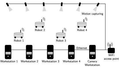
Figure 3: Experimental setup. The DMPC controllers run on the workstation computers and each robot is assigned one workstation to run Algorithm 1.

4.2 DMPC Implementation

We have implemented Algorithms 1–3 in C++ and the source code is available online. Besides the C++ standard library, our implementation relies on four external libraries: (i) Eigen to store vectors and matrices as well as to regularize $H_{i}$; (ii) qpOASES (Ferreau et al., 2014) to solve the subsystem QPs; (iii) CasADi (Andersson et al., 2019) to evaluate sensitivities in dSQP via automatic differentiation; and (iv) LCM to exchange optimizer iterates with neighbors.

While our implementation uses dynamic memory, we allocate any dynamic memory prior to running the control loop, thus accelerating the execution time of our methods.

For Step 3 in Algorithm 2 and for Step 6 in Algorithm 3, we use the online active-set method implemented in qpOASES. We initialize the QP solver once prior to running the DMPC controller, and solely use the efficient hotstart procedure online to update the current and desired robot positions.

All communication of the algorithms happens via the aforementioned LCM library. There, communication follows a publish-subscribe pattern. Messages are received and cached asynchronously by a separate thread of the solver program, with the data being accessed when required by the algorithm. If a required piece of data has not yet been received and cached, the algorithm waits until all data necessary to continue calculations is available. For state measurements to be received, a maximum waiting time can be set so that the algorithm does not wait indefinitely if a state measurement has been lost. For optimizer iterates, however, lost messages are resent by the control application to ensure a synchronous execution of ADMM. This is necessary since we rely on UDP and not on the transmission control protocol as (Burk et al., 2021b).

The main thread of each DMPC program sleeps after Step 6 of Algorithm 1. To reduce the effect of jitter, we implement the sleep via std::this_thread::sleep_until. This is crucial to ensure that all controllers keep the same sampling interval $\Delta t$ in the distributed setting.

5 Experimental Results

5.1 Formation Control via linear-quadratic MPC and ADMM

We consider a scenario where a set $\mathcal{S}=\{1,2,3,4\}$ of four mobile robots moves in a chain-like formation. OCP (1) is designed such that each robot is coupled to its neighbors in the chain, i.e., the underlying coupling and communication graph is a path graph of length four. The robots are initially positioned with an equidistant spacing of $0.4\,\mathrm{m}$. The first robot then moves along a rectangular path and the remaining robots follow while keeping the initialized distance to their neighbors. Figure 4 summarizes the control architecture and shows the communicated signals between robots and controllers.

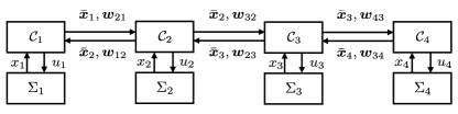
Figure 4: Block diagram for a path graph of four robots $\Sigma_{i}$. The controllers $\mathcal{C}_{i}$ of neighboring robots exchange predicted position trajectories $\bar{\boldsymbol{x}}_{i}$ and $\boldsymbol{w}_{ij}$.

We choose a horizon $N=7$ and a sampling interval ${\Delta t=0.2\,\text{s}}$. For the cost matrices, we set $Q_{11}=Q_{22}=Q_{33}=\text{diag}(20,20)$, $Q_{44}=\text{diag}(10,10)$, $Q_{ij}=\text{diag}(-10,-10)$ for all $j\in\{i-1,i+1\}\cap\mathcal{S}$ and for all $i\in\mathcal{S}$, and $R_{ii}=\text{diag}(1,1)$ for all $i\in\mathcal{S}$. The remaining cost matrices $Q_{ij}$ are set to zero. The terminal cost matrix is chosen as $P=Q$. The setpoints are $\bar{x}_{1}=x_{1}^{\text{d}}(t)$ and $\bar{x}_{i}=\bar{x}_{i-1}+\delta$ for all $i\in\{2,3,4\}$, where $x_{1}^{\text{d}}(t)$ encodes the rectangular path and ${\delta=\begin{bmatrix}-0.4&0\end{bmatrix}^{\top}\,\mathrm{m}}$ is the desired spacing between neighbors. The input constraints are given as ${\begin{bmatrix}-0.2&-0.2\end{bmatrix}^{\top}\,\mathrm{m/s}\leq u_{i}\leq\begin{bmatrix}0.2&0.2\end{bmatrix}}^{\top}\,\mathrm{m/s}$ for all $i\in\mathcal{S}$. We enforce no state constraints such that $\mathbb{X}_{i}=\mathbb{R}^{n_{x,i}}$ and $\mathbb{X}_{ij}=\mathbb{R}^{n_{x,i}}\times\mathbb{R}^{n_{x,j}}$ for all $i,j\in\mathcal{S}$. OCP (1) therefore is a strongly convex QP.

Figure 5: Rectangle scenario using ADMM-based DMPC: camera images and rectangular path (dashed line), robot one trajectory (solid blue line), and current formation (solid orange line).

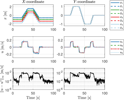
Figure 6: Rectangle scenario using ADMM-based DMPC: closed-loop position $x$ and velocity $u$ trajectories and optimizer residual.

For ADMM, we empirically tune $\rho$ in the range $\{0.1,1,10,100\}$ for fastest convergence to the OCP minimizer and choose $\rho=1$. We fix the number of ADMM iterations executed per MPC step to five. That is, we set $l_{\mathrm{max}}=5$ in Algorithm 2. Moreover, we warm-start ADMM and set $\bar{z}^{0}$ and $\gamma^{0}$ to the solution obtained in the prior MPC step shifted by the time index. In the first MPC step, we set $\bar{z}^{0}=\gamma^{0}=0$.

A video recording of the experiment is available in the digital supplementary material of the article and selected still images from the experiment are shown in Figure 5. The camera videos and still images are undistorted via suitable image processing algorithms. The robot positions are superimposed onto the images using mapped data recorded by the tracking system. Figure 5 shows the robot positions in the $X,Y-$plane, but not the heading angle. This is because the robots are omnidirectional and hence the system dynamics do not depend on the robot orientation.

Figure 6 shows the closed-loop state and input trajectories for the individual robots as well as the residual $\|u-u^{\star}\|_{\infty}$ between the applied input $u$ and the centralized optimal solution $u^{\star}$ obtained from IPOPT (Wächter and Biegler, 2006). Plots in the left and right columns of Figure 6 present the motion in the $X$- and $Y$-coordinates, respectively. The plots in the top row show that the control scheme is able to track the desired setpoint accurately. As can be seen from the bottom plot, ADMM produces input signals which deviate less than $2\cdot 10^{-2}\,\mathrm{m/s}$ from the optimal solution once an initialization phase of a few seconds has passed. This confirms previous results in the sense that a low number of ADMM iterations per control step can suffice in practice to obtain a reasonable control performance (Van Parys and Pipeleers, 2017; Burk et al., 2021b; Stomberg et al., 2022a).

Table 2 shows the median and maximum execution times for ADMM per MPC step and the execution time per ADMM iteration. The data reported therein is based on two experiments with a total duration of approximately three minutes. The robots took at most $22.27\,\mathrm{ms}$ to execute ADMM per MPC step. Since this is well below the control sampling interval $\Delta t$, and since we compensate for the computational delay by solving OCP (1) for $u(t+\Delta t)$, our implementation is sufficiently fast to execute the DMPC scheme in real-time.

Table 2: ADMM execution time broken into the steps of Algorithm 2. The robots take less than 23 ms to solve OCP (1) in each MPC step. This is below the 200 ms sampling interval and demonstrates the real-time capabilities of the implementation.

	Median [ms]	Max. [ms]
Solve OCP with ADMM	6.61	22.27
Time per ADMM iteration	0.98	16.71
Solve subsystem QP (Step 3)	0.09	14.57
Communicate $z$ (Steps 4–5)	0.29	11.92
Communicate $\bar{z}$ (Step 6)	0.25	11.63

In addition to the overall ADMM execution time, we are interested in the time required for Steps 3, 4, and 6 of Algorithm 2. Table 2 therefore further shows the median and maximum time spans the robots spent on these individual steps. The time given for Steps 4 and 6 includes the following five substeps: (i) write the variables into an LCM message, (ii) publish the LCM message, (iii) wait for messages sent by neighbors, (iv) write the received variables into local data structures, and (v) if necessary, resend messages to neighbors. For Step 4, the time span also includes computing the average in Step 5. Table 2 shows that, in most cases, solving the subsystem QP with qpOASES is significantly faster than exchanging trajectories with neighbors.

As another metric for the execution time, we analyze how much time each robot has spent solving the subsystem QP and communicating/waiting. Table 3 reports the time each robot spent in Steps 3 and Steps 4–6 compared to the total time it spent running ADMM. All robots spent more time communicating or waiting for their neighbors than solving their quadratic subproblem. Even though all subproblem QPs have the same structure, robots three and four take less time in Step 3 of Algorithm 2 than robots one and two. This is due to performance differences between the workstation computers used to run the DMPC controller for robots three and four compared to robots one and two.

Table 3: Fraction of the ADMM execution time spent on Steps 3, 4, and 6 of Algorithm 2. Differences between individual robots originate from the varying computational power of the employed hardware.

Robot	1	2	3	4
Solve subsystem QP (Step 3)	37 %	33 %	15 %	16 %
Communicate (Steps 4–6)	62 %	66 %	85 %	84 %

5.2 Non-convex Minimum-distance Constraints and dSQP

The DMPC scheme discussed in the previous subsection relies on cost coupling to meet the formation control specifications. In this section, we additionally enforce a minimum-distance constraint between neighbors such that for all ${i\in\{2,3,4\}}$ we enforce coupled state constraints

$$\mathbb{X}_{ij}=\left\{x_{i}\in\mathbb{R}^{2}\times x_{j}\in\mathbb{R}^{2}\,\big{|}\,\left\|x_{i}-x_{j}\right\|_{2}^{2}\geq d\right\},$$ (8)

where $j=i-1$ and $d=0.4\,\mathrm{m}$. Therefore, OCP (1) here is a non-convex quadratically constrained quadratic program (QCQP), where the distance constraint (8) is included in the subsystem inequality constraints (2c) of robots two to four.

We soften the collision avoidance constraints as described in Remark 2 and we solve the soft OCP with dSQP. To this end, we run five SQP iterations per MPC step and three ADMM iterations per SQP iteration. That is, we set $q_{\mathrm{max}}=5$ and ${l_{\mathrm{max}}=3}$ in Algorithm 3. We again tune $\rho$ in the range $\{0.1,1,10,100\}$ and choose $\rho=1$. As for ADMM, we warm-start Algorithm 3 and set $z^{0}$ and $\gamma^{0}$ to the shifted values obtained in the previous MPC step. We use the Gauss-Newton Hessian approximation $H_{i}=\nabla_{z_{i}z_{i}}^{2}f_{i}$ and therefore omit an initialization for $\nu$ and $\mu$.

A video recording of the experiment is provided in the digital supplementary material and still images of the experiment are depicted in Figure 7. Figure 8 shows closed-loop state and input trajectories as well as the dSQP input residual. In the first 20 seconds of the experiment, the robots leave the chain formation and spread across the room. Then, from $t=20\,\mathrm{s}$ onwards, they return to the chain formation. This maneuver is more challenging than driving along the rectangular shape, as it requires robots two and three to switch their position while avoiding a collision. In fact, the shown maneuver cannot be carried out using the ADMM-based DMPC scheme without distance constraints presented in the previous section since simulations indicate that robots two and three would collide.

The bottom plots in Figure 8 show the residual $\|u-u^{\star}\|_{\infty}$ between the applied input $u$ determined by dSQP and the local optimum $u^{\star}$ found when solving the OCP in centralized fashion via IPOPT. The control input found by dSQP differs significantly from the IPOPT solution when the experiment begins and when the setpoint changes. This is because we lack a good warm-start in these situations. However, dSQP returns nearly optimal inputs during the transient phases and upon convergence of the controlled system.

Figure 7: Formation change scenario using dSQP-based DMPC: camera images and formation one (green crosses), formation two (red crosses), and current formation (solid orange line).

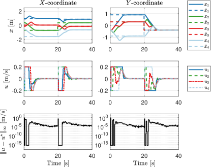
Figure 8: Formation change scenario using dSQP-based DMPC: closed-loop position $x$ and input $u$ trajectories and optimizer residual.

Table 4 summarizes the execution times measured in twelve experiments with a total duration of 12 minutes. The OCP was solved by dSQP in less than $54\,\mathrm{ms}$ and the implementation is hence sufficiently fast. The table further presents the execution time for the most expensive steps of Algorithm 3. Since the Gauss-Newton Hessian approximation $H_{i}=\nabla_{z_{i}z_{i}}^{2}f_{i}$ can be evaluated offline, Step 3 of Algorithm 3 is cheap. In fact, Algorithm 3 spends most time executing ADMM in Steps 5–13.

Table 4: dSQP execution time broken into the steps of Algorithm 3. The robots take less than 54 ms to solve OCP (1) in each MPC step. This is well below the 200 ms sampling interval and demonstrates the real-time capabilities of the implementation.

	Median [ms]	Max. [ms]
Solve OCP with dSQP	33.81	53.06
Time per dSQP iteration	6.23	24.57
Build subsystem QP (Step 3)	0.30	1.09
Run ADMM per dSQP iter	5.99	24.29
Time per ADMM iteration	2.01	15.37
Solve subsystem QP (Step 6)	0.81	12.40
Communicate $z$ (Step 7–8)	0.64	12.17
Communicate $\bar{z}$ (Step 9)	0.32	11.53

Table 5 shows the fraction of the dSQP execution time each robot spent on building and solving the subsystem QP and on communicating with neighbors. Compared to Table 3, robots two to four spent more time in Table 5 on solving the subsystem QP due to the added distance constraint. In particular, robot two spent more time solving the subsystem QP than communicating or waiting.

Table 5: Fraction of the dSQP execution time spent on Steps 3, 6, 7, and 9 of Algorithm 3. Due to the minimum-distance constraint and comparatively weaker hardware, robot two spends more time solving the subsystem QPs than communicating trajectories to robots one and three.

Robot	1	2	3	4
Build subsystem QP (Step 3)	5 %	5 %	3 %	4 %
Solve subsystem QP (Step 6)	34 %	68 %	42 %	29 %
Communicate (Steps 7–9)	60 %	26 %	55 %	65 %

5.3 Discussion

The experiments demonstrate the effectiveness of the controller design and of our implementation and the results show that control sampling intervals in the millisecond range can be achieved by cooperative DMPC schemes. Depending on the OCP structure and the optimization method, both subsystem computations and communication steps can take a substantial part of the execution time. This is in contrast to (Van Parys and Pipeleers, 2017), where subsystem computations are a clear bottleneck, as well as to (Burk et al., 2021b), where communication is holding up. Warm-starting the optimization methods in DMPC allows to find a reasonable control input with only few optimizer iterations per MPC step.

Despite the promising performance in the experiments with respect to control performance and execution time, there are limitations to our approach. First, we lack rigorous recursive feasibility and convergence guarantees for the control loop because we do not design tailored terminal ingredients for the OCP. To obtain such theoretial guarantees, one could follow the design procedure presented in (Darivianakis et al., 2019). However, this would only be possible for the scenario without the non-convex distance constraints, as the design in (Darivianakis et al., 2019) only applies to subsystems coupled through polytopic constraints. Second, the employed dSQP variant is not guaranteed to converge to an OCP minimizer as we fix the number of ADMM iterations executed per SQP iteration instead of terminating ADMM dynamically. To obtain local convergence guarantees, one could incorporate a stopping criterion into Algorithm 3 (Stomberg et al., 2022b). This would imply varying optimizer iterations per control step and the additional communication of convergence flags. Third, our implementation and computing hardware is not hard real-time capable. That is, even though the observed OCP solution times were strictly shorter than the control sampling intervals, we cannot formally guarantee a sufficiently fast execution of our optimization methods. Hard real-time guarantees could be obtained by implementing the approaches for execution on microcontrollers or field programmable gate arrays (McInerney et al., 2018).

6 Conclusion

This article presented experimental results for iterative DMPC schemes based on ADMM and dSQP as well as insights into their efficient implementation for real-time execution. The decentralized implementation controlled a team of four mobile robots moving in formation. A dedicated stationary computer was assigned to each robot to run the DMPC application. The employed decentralized optimization methods ADMM and dSQP solved the centralized OCP sufficiently fast and the DMPC scheme compensated for the computational delay. In particular, dSQP solved non-convex distance constraints online to avoid collisions between robots. Future work will consider control schemes with formal stability guarantees, an implementation with hard real-time capabilities, and robots with more sophisticated dynamics, e.g., due to non-holonomic constraints.

References

- Andersson et al. (2019) Andersson, J.A.E., Gillis, J., Horn, G., Rawlings, J.B., Diehl, M., 2019. CasADi: A software framework for nonlinear optimization and optimal control. Mathematical Programming Computation 11, 1–36. doi:10.1007/s12532-018-0139-4.
- Bai et al. (2011) Bai, H., Arcak, M., Wen, J., 2011. Cooperative control design: a systematic, passivity-based approach. Springer Science+Business Media, New York. doi:10.1007/978-1-4614-0014-1.
- Bertsekas and Tsitsiklis (1989) Bertsekas, D.P., Tsitsiklis, J.N., 1989. Parallel and Distributed Computation: Numerical Methods. volume 23. Prentice Hall, Englewood Cliffs, NJ.
- Bestler and Graichen (2019) Bestler, A., Graichen, K., 2019. Distributed model predictive control for continuous-time nonlinear systems based on suboptimal ADMM. Optimal Control Applications and Methods 40, 1–23. doi:10.1002/oca.2459.
- Bock (1983) Bock, H.G., 1983. Recent advances in parameteridentification techniques for ODE, in: Deuflhard, P., Hairer, E. (Eds.), Numerical treatment of inverse problems in differential and integral equations. Birkhäuser Boston, Boston, MA, pp. 95–121. doi:10.1007/978-1-4684-7324-7_7.
- Boyd et al. (2011) Boyd, S., Parikh, N., Chu, E., Peleato, B., Eckstein, J., 2011. Distributed optimization and statistical learning via the alternating direction method of multipliers. Foundations and Trends in Machine Learning 3, 1–122. doi:10.1561/2200000016.
- Burk et al. (2021a) Burk, D., Völz, A., Graichen, K., 2021a. Experimental validation of the open-source DMPC framework GRAMPC-D applied to the remotely accessible robotarium, in: Proceedings of the IEEE International Conference on Mechatronics and Automation (ICMA), pp. 442–447. doi:10.1109/ICMA52036.2021.9512773.
- Burk et al. (2021b) Burk, D., Völz, A., Graichen, K., 2021b. A modular framework for distributed model predictive control of nonlinear continuous-time systems (GRAMPC-D). Optimization and Engineering 23, 771–795. doi:10.1007/s11081-021-09605-3.
- Conte et al. (2016) Conte, C., Jones, C.N., Morari, M., Zeilinger, M.N., 2016. Distributed synthesis and stability of cooperative distributed model predictive control for linear systems. Automatica 69, 117–125. doi:10.1016/j.automatica.2016.02.009.
- Conte et al. (2012) Conte, C., Summers, T., Zeilinger, M.N., Morari, M., Jones, C.N., 2012. Computational aspects of distributed optimization in model predictive control, in: Proceedings of the 51st IEEE Conference on Decision and Control, pp. 6819–6824. doi:10.1109/CDC.2012.6426138.
- Darivianakis et al. (2019) Darivianakis, G., Eichler, A., Lygeros, J., 2019. Distributed model predictive control for linear systems with adaptive terminal sets. IEEE Transactions on Automatic Control 65, 1044–1056.
- Ebel and Eberhard (2021) Ebel, H., Eberhard, P., 2021. A comparative look at two formation control approaches based on optimization and algebraic graph theory. Robotics and Autonomous Systems 136, 103686. doi:10.1016/j.robot.2020.103686.
- Ebel and Eberhard (2022) Ebel, H., Eberhard, P., 2022. Cooperative transportation: realizing the promises of robotic networks using a tailored software/hardware architecture. at – Automatisierungstechnik 70, 378–388. doi:10.1515/auto-2021-0105.
- Ebel et al. (2017) Ebel, H., Sharafian Ardakani, E., Eberhard, P., 2017. Comparison of distributed model predictive control approaches for transporting a load by a formation of mobile robots, in: Proceedings of the 8th Eccomas Thematic Conference on Multibody Dynamics, Prague. doi:10.18419/opus-10734.
- Engelmann et al. (2021) Engelmann, A., Benner, H., Ou, R., Jiang, Y., Faulwasser, T., Houska, B., 2021. ALADIN-—A rapid-prototyping toolbox for distributed and decentralized non-convex optimization. Optimal Control: Applications and Methods 43, 4–22. doi:10.1002/oca.2811.
- Engelmann et al. (2020) Engelmann, A., Jiang, Y., Houska, B., Faulwasser, T., 2020. Decomposition of nonconvex optimization via bi-level distributed ALADIN. IEEE Transactions on Control Network Systems 7, 1848–1858. doi:10.1109/TCNS.2020.3005079.
- Eschmann et al. (2021) Eschmann, H., Ebel, H., Eberhard, P., 2021. Trajectory tracking of an omnidirectional mobile robot using Gaussian process regression. at – Automatisierungstechnik 69, 656–666. doi:10.1515/auto-2021-0019.
- Ferreau et al. (2014) Ferreau, H.J., Kirches, C., Potschka, A., Bock, H.G., Diehl, M., 2014. qpOASES: A parametric active-set algorithm for quadratic programming. Mathematical Programming Computation 6, 327–363. doi:10.1007/s12532-014-0071-1.
- Findeisen (2006) Findeisen, R., 2006. Nonlinear Model Predictive Control: A Sampled-data Feedback Perspective. Fortschritt-Berichte VDI: Reihe 8, VDI-Verlag.
- Giselsson and Rantzer (2014) Giselsson, P., Rantzer, A., 2014. On feasibility, stability and performance in distributed model predictive control. IEEE Transactions on Automatic Control 59, 1031–1036. doi:10.1109/TAC.2013.2285779.
- Grau et al. (2017) Grau, A., Indri, M., Bello, L.L., Sauter, T., 2017. Industrial robotics in factory automation: From the early stage to the internet of things, in: Proceedings of the IECON 2017 – 43rd Annual Conference of the IEEE Industrial Electronics Society, Beijing. pp. 6159–6164. doi:10.1109/IECON.2017.8217070.
- Gu and Yang (2005) Gu, D., Yang, E., 2005. A suboptimal model predictive formation control, in: Proceedings of the IEEE/RSJ International Conference on Intelligent Robots and Systems, pp. 1295–1300. doi:10.1109/IROS.2005.1545536.
- He and Yuan (2012) He, B., Yuan, X., 2012. On the O(1/n) convergence rate of the Douglas–Rachford alternating direction method. SIAM Journal on Numerical Analysis 50, 700–709. doi:10.1137/110836936.
- Huang et al. (2010) Huang, A.S., Olson, E., Moore, D.C., 2010. LCM: Lightweight communications and marshalling, in: Proceedings of the 2010 IEEE/RSJ International Conference on Intelligent Robots and Systems, Taipei. pp. 4057–4062. doi:10.1109/IROS.2010.5649358.
- Kanjanawanishkul and Zell (2008) Kanjanawanishkul, K., Zell, A., 2008. A model-predictive approach to formation control of omnidirectional mobile robots, in: Proceedings of the IEEE/RSJ International Conference on Intelligent Robots and Systems, pp. 2771–2776. doi:10.1109/IROS.2008.4650752.
- Köhler et al. (2019) Köhler, J., Müller, M.A., Allgöwer, F., 2019. Distributed model predictive control—recursive feasibility under inexact dual optimization. Automatica 102, 1–9. doi:10.1016/j.automatica.2018.12.037.
- Kuwata et al. (2007) Kuwata, Y., Richards, A., Schouwenaars, T., How, J.P., 2007. Distributed robust receding horizon control for multivehicle guidance. IEEE Transactions on Control Systems Technology 15, 627–641. doi:10.1109/TCST.2007.899152.
- Maciejowski (2002) Maciejowski, J.M., 2002. Predictive control with constraints. Pearson Education, Harlow.
- McInerney et al. (2018) McInerney, I., Constantinides, G.A., Kerrigan, E.C., 2018. A survey of the implementation of linear model predictive control on FPGAs. IFAC-PapersOnLine 51, 381–387.
- Müller and Allgöwer (2017) Müller, M.A., Allgöwer, F., 2017. Economic and distributed model predictive control: recent developments in optimization-based control. SICE Journal of Control, Measurement, and System Integration 10, 39–52. doi:10.9746/jcmsi.10.39.
- Nedić et al. (2018) Nedić, A., Olshevsky, A., Rabbat, M.G., 2018. Network topology and communication-computation tradeoffs in decentralized optimization. Proceedings of the IEEE 106, 953–976. doi:10.1109/JPROC.2018.2817461.
- Novoth et al. (2021) Novoth, S., Zhang, Q., Ji, K., Yu, D., 2021. Distributed formation control for multi-vehicle systems with splitting and merging capability. IEEE Control Systems Letters 5, 355–360. doi:10.1109/LCSYS.2020.3002218.
- Olfati-Saber et al. (2007) Olfati-Saber, R., Fax, J.A., Murray, R.M., 2007. Consensus and cooperation in networked multi-agent systems. Proceedings of the IEEE 95, 215–233. doi:10.1109/JPROC.2006.887293.
- Rosenfelder et al. (2022) Rosenfelder, M., Ebel, H., Eberhard, P., 2022. Cooperative distributed nonlinear model predictive control of a formation of differentially-driven mobile robots. Robotics and Autonomous Systems 150, 103993. doi:10.1016/j.robot.2021.103993.
- Rostami et al. (2017) Rostami, R., Costantini, G., Görges, D., 2017. ADMM-based distributed model predictive control: primal and dual approaches, in: Proceedings of the 56th IEEE Conference on Decision and Control, pp. 6598–6603. doi:10.1109/CDC.2017.8264654.
- Scattolini (2009) Scattolini, R., 2009. Architectures for distributed and hierarchical model predictive control – a review. Journal of Process Control 19, 723–731. doi:10.1016/j.jprocont.2009.02.003.
- Stewart et al. (2011) Stewart, B.T., Wright, S.J., Rawlings, J.B., 2011. Cooperative distributed model predictive control for nonlinear systems. Journal of Process Control 21, 698–704. doi:10.1016/j.jprocont.2010.11.004.
- Stomberg et al. (2022a) Stomberg, G., Engelmann, A., Faulwasser, T., 2022a. A compendium of optimization algorithms for distributed linear-quadratic MPC. at - Automatisierungstechnik 70, 317–330. doi:10.1515/auto-2021-0112.
- Stomberg et al. (2022b) Stomberg, G., Engelmann, A., Faulwasser, T., 2022b. Decentralized non-convex optimization via bi-level SQP and ADMM, in: Proceedings of the 61st IEEE Conference on Decision and Control (CDC), pp. 273–278. doi:10.1109/CDC51059.2022.9992379.
- Van Parys and Pipeleers (2017) Van Parys, R., Pipeleers, G., 2017. Distributed MPC for multi-vehicle systems moving in formation. Robotics and Autonomous Systems 97, 144–152. doi:10.1016/j.robot.2017.08.009.
- Venkat et al. (2008) Venkat, A.N., Hiskens, I.A., Rawlings, J.B., Wright, S.J., 2008. Distributed MPC strategies with application to power system automatic generation control. IEEE Transactions on Control Systems Technology 16, 1192–1206. doi:10.1109/TCST.2008.919414.
- Wächter and Biegler (2006) Wächter, A., Biegler, L.T., 2006. On the implementation of an interior-point filter line-search algorithm for large-scale nonlinear programming. Mathematical Programming 106, 25–57. doi:10.1007/s10107-004-0559-y.
- Wang et al. (2019) Wang, Y., Yin, W., Zeng, J., 2019. Global convergence of ADMM in nonconvex nonsmooth optimization. Journal of Scientific Computing 78, 29–63. doi:10.1007/s10915-018-0757-z.
- Wen et al. (2018) Wen, J., He, L., Zhu, F., 2018. Swarm robotics control and communications: Imminent challenges for next generation smart logistics. IEEE Communications Magazine 56, 102–107. doi:10.1109/MCOM.2018.1700544.
- Yan and Bitmead (2003) Yan, J., Bitmead, R., 2003. Coordinated control and information architecture, in: Proceedings of the 42nd IEEE International Conference on Decision and Control, pp. 3919–3923. doi:10.1109/CDC.2003.1271762.