Belief propagation on networks with cliques and chordless cycles
Abstract
It is well known that tree-based theories can describe the properties of undirected clustered networks with extremely accurate results [S. Melnik, et al. Phys. Rev. E 83, 036112 (2011)]. It is reasonable to suggest that a motif based theory would be superior to a tree one; since additional neighbour correlations are encapsulated in the motif structure. In this paper we examine bond percolation on random and real world networks using belief propagation in conjunction with edge-disjoint motif covers. We derive exact message passing expressions for cliques and chordless cycles of finite size. Our theoretical model gives good agreement with Monte Carlo simulation and offers a simple, yet substantial improvement on traditional message passing showing that this approach is suitable to study the properties of random and empirical networks.
pacs:
Valid PACS appear hereI Introduction
Belief propagation, also known as message passing, is an algorithm that is fundamental to many different disciplines including physics, computer science, epidemiology and statistics yedidia_freeman_weiss_2005 ; newman_2019 ; cantwell_newman_2019 ; kirkley_cantwell_newman_2021 ; mezard_parisi_zecchina_2002 ; PhysRevE.56.1357 ; michaelbeyond2022 ; bodnar2021weisfeiler . The belief propagation algorithm, which relies on the Bethe-Peierls approximation bethe_1935 ; 8262801 ; WellerEtAl_uai14 , is valid only for large and sparse treelike networks; becoming exact when the network is a tree. This is because the removal of a vertex, , and its edges from a tree isolates its neighbours from one another; the only path connecting them has vanished and so too do inter-neighbour correlations. Such a graph is called the cavity graph of vertex and allows a message passing system of self-consistent equations to be written for the vertices of the network. Loops in networks introduce correlations between vertices that invalidates the Bethe-Peierls approximation as there is still a path between the neighbours in the cavity graph of a given vertex. Despite this drawback, belief propagation has a proven ability to analytically describe the structural properties of many real world networks, which are known to contain loops PhysRevLett.113.208702 . Belief propagation on clustered networks has been studied previously yedidia_freeman_weiss_2005 ; Gujrati_2001 ; PhysRevB.71.235119 ; PhysRevE.82.036101 ; PhysRevE.84.055101 ; PhysRevE.84.041144 ; PhysRevE.100.012314 ; PhysRevLett.113.208701 ; Coolen_2016 ; kirkley_cantwell_newman_2021 ; NIPS1997_0245952e ; cantwell_newman_2019 ; PhysRevE.99.042309 ; michaelbeyond2022 ; bodnar2021weisfeiler ; PhysRevE.73.065102 and an immense literature exists that tackles the problem in a variety of different manners.
Recently, Cantwell, Newman and Kirkley solved the belief propagation model for networks with arbitrary loop structure kirkley_cantwell_newman_2021 ; cantwell_newman_2019 . They achieved this by considering messages from a collective local neighbourhood, of variable distance, about each vertex, rather than a partition into recognised motifs. In their framework, it is assumed that all inter-vertex correlations due to short range loops are encapsulated within the neighbourhood. For a given configuration of edges, the probability of the size of the component to which a vertex belongs is calculated, before being averaged over the probability of each edge configuration for the neighbourhood. The neighbourhood calculation is computationally expensive and so the authors introduced a Monte Carlo algorithm to sample the set of connected graphs.
It is not unreasonable, however, to desire a model of an empirical network to carry out further experimentation on. For instance, suppose that the empirical network represents a data set that is too small to apply some statistical or machine learning algorithm. If we had a model of the network, perhaps we could understand how to grow the network, adding new vertices and edges, whilst keeping the inherent topology and statistical properties fixed.
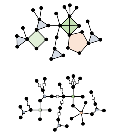
One way to obtain a model is to cover the network in motifs; specifically, a set of edge-disjoint motifs, such that a given edge belongs to only one motif. The simplest cover is to simply assume each edge is a 2-clique PhysRevLett.113.208702 - and this approximation certainly works well in some cases. However, given the large body of knowledge for random clustered networks PhysRevLett.103.058701 ; PhysRevE.80.020901 ; karrer_newman_2010 ; PhysRevE.101.062310 ; PhysRevE.105.044314 ; PhysRevE.104.024304 ; PhysRevE.103.012313 ; PhysRevE.103.012309 ; PhysRevE.84.041144 ; burgio_arenas_gomez_matamalas_2021 ; HASEGAWA2021125970 it is tempting to apply covers with larger and more complicated motifs in the hope to obtain more accurate models. For sparse random graphs, this technique works well and the success lies in the locally treelike nature of the factor graph of the covered network. The factor graph is a bipartite graph that has two different sets of vertices. One set represents the vertices of the substrate network, whilst the other represents the motifs to which they belong. Edges connect vertices in the original graph to the vertices representing the motifs to which they belong, see Fig 1. If the factor graph is locally treelike then all of the short range loops in the network are encapsulated within the motif cover.
Unfortunately, naive motif covers of empirical networks often do not create representative models. Cantwell, Kirkley and Newman summarise that “these techniques are not generally applicable to real world networks” kirkley_cantwell_newman_2021 . In fact, it is sometimes the case that tree-based theories give the closest match to the empirical network. This is despite a cover with larger motifs necessarily having a more treelike factor graph than a cover comprised of only 2-cliques. This indicates the presence of an additional driving force for a suitable motif cover beyond simply decreasing the number of loops in the factor graph.
In this paper, we introduce exact expressions for belief propagation on random networks that are composed of chordless cycles and cliques of finite size. We then study message passing on empirical clique covered networks. We find that our model exhibits excellent agreement with Monte Carlo simulation beyond the results obtained from ordinary belief propagation PhysRevLett.113.208702 due to the arbitrarily large clique sizes we can analytically include in our model. We offer insight into why naive motif covers often fail to capture the properties of real world networks by considering the statistical bias introduced by the breaking of symmetry in certain covers. Finally, we relate our method to the generalised configuration model which is shown to be the ensemble average of the message passing model.
This work will lead to significant advances in the application of the theory of clustered graphs to the study of empirical networks. We hope that additional studies will be conducted with dynamics other than bond percolation to further these results.
II Theoretical
Let be a graph, and be a edge configuration on the graph that maps each edge to a value of either 0 or 1 with probabilities and , respectively for . An edge is occupied if for , and unoccupied if ; as is increased a giant connected component of occupied edges emerges through a phase transition. The state space of the model is such that are -dimensional vectors. Let denote the set of occupied edges. For a given network the probability measure of an edge configuration is
| (1) |
where is the partition function
| (2) |
This summation is over all possible edge configurations of a given graph, weighted by their probabilities and therefore, is equal to one. When is small, the graph is composed of many small clusters of occupied vertices and there is no long range connectivity. As is increased a giant percolating cluster emerges which incorporates a finite fraction of the vertices .
We now derive the belief propagation formulation for motif covered networks. Similar expressions appear in cantwell_newman_2019 for vertex neighbourhood decompositions; and PhysRevE.84.041144 for the Ising model on motif covered networks. Let us select a vertex at random from the equilibrium of the percolation process and suppose that is the corner of a set of motifs . The probability is the probability that belongs to a non-percolating component of size . This can be written in terms of the probability that a neighbour of , vertex , which is in motif together with , leads to vertices if we were to follow all of its edges, other than those that point back to motif
| (3) |
where is a motif belonging to , is the set of edges vertex has within motif and where is the Kronecker delta. This expression averages over every combination of the total number of reachable vertices along each edge of each motif in the set of motifs that belongs to. This summation is then filtered by the Kronecker delta to retain only those terms that collectively sum to , to which we add 1 for vertex itself to yield the component of overall size . We can generate this probability by defining
| (4) |
such that
| (5) |
With the following manipulation
| (6) |
we obtain
| (7) |
The summation limits over are ; since, the original summation is over and so is . For each neighbour we can write a generating function for the probability that the number of vertices that can be reached, other than through the motif itself, is as
| (8) |
The probability for the total number of vertices that can be reached via motif is simply the product
| (9) |
Inserting these expressions in Eq 7 we find
| (10) |
This expression is a general result and holds for arbitrary motif topologies. If we had knowledge of each this generating function would yield the distribution of component sizes that vertex belongs to. From this, for instance, we can find the size of the percolating component as one minus the probability that all vertices belong to finite components
| (11) |
The average size of the finite components is given by
| (12) |
where we have used Eq 4. Inserting Eq 10 we have
| (13) |
where we have used
| (14) |
To progress we require the derivative of . However, the functional form of , crucial to enumerating , depends on the structure of the motif and the configuration of its edges among the occupied and unoccupied states. We will now examine for ordinary edges, chordless cycles of arbitrary length and cliques of arbitrary size.
II.1 Calculating for ordinary edges
Let us for a moment assume that the network contains only 2-cliques - ordinary edges; which was previously studied by Karrer et al PhysRevLett.113.208702 . In this case Eq 10 reduces to
| (15) |
where the product over accounts for each distinct 2-clique belongs to. Because there is only a single edge in a 2-clique, this index equivalently runs over the neighbour vertices . If the edge is unoccupied with probability , then is zero. In this case, the edge does not contribute to the component size of and so . If the edge is occupied with probability , then is non-zero. Therefore, the summation in Eq 8 has the zero term extracted, and for we have
| (16) |
where the notation denotes the set edges to which vertex belongs to excluding the one connecting it to . Substituting this expression into Eq 8 we have
| (17) |
Application of the Kronecker delta yields
| (18) |
Noticing that the final summation is the generating function of (Eq 8) we have a self-consistent expression for
| (19) |
This expression can be solved for all edges by fixed point iteration from a suitable starting point and substituted into Eq 10 to find . The distribution for can then be found by differentiating the series.
To evaluate the finite components, we require the derivative of with respect to . Following PhysRevLett.113.208702 we find
| (20) |
To find the average size of the finite components we solve Eqs 19 and 20 and insert them into Eq 13.
II.2 Calculating for 3-cliques
Let us now examine the case where vertices belong to triangles as well as ordinary edges. Each triangle that vertex belongs to connects it to vertices and ; and, our aim is to calculate the generating function for the probability that the number of vertices that are reachable from vertex due to its membership in triangle is . However, unlike ordinary edges, which contain just 1 edge, a triangle has 3 edges. Each of these edges may be occupied , or unoccupied and there are 7 distinct edge configurations for a given triangle that bear impact on the connectivity of vertex , see Fig 2.
The probability that the triangle connects to vertices is dependent on the edge configuration that the triangle is in. Therefore, in order to compute , we must calculate conditional probabilities of leading to vertices for a given edge configuration . We find
| (21a) | ||||
| (21b) | ||||
| (21c) | ||||
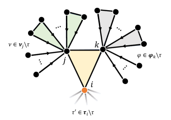
where the notation in Eq 21b denotes the set of motifs that vertex belongs to excluding ; and similarly for in Eq 21c. When the focal vertex is connected to both and in via occupied edges, we must average over both sets of neighbours, see Fig 3.
| (22) |
The total probability that triangle leads to vertices is found by summing each conditional probability with the probability of each edge configuration PhysRevLett.103.058701 ; karrer_newman_2010 ; PhysRevE.104.024304
| (23) |
Extracting the term, we generate this expression as
| (24) |
Summing over , expressions 21b and 21c follow similar manipulations to Eq 6; whilst Eq 22 becomes
| (25) |
The Kronecker delta evaluates as follows
| (26) | ||||
| (27) |
We find
| (28) | ||||
| (29) |
Inserting this result into Eq 24 together with the other expressions in Eqs 21b and 21c we have
| (30) |
The result is a polynomial in powers of generating functions where is a vertex in motif and is a motif that belongs to, other than motif .
II.3 Calculating for chordless cycles of size
Perhaps the simplest family of subgraphs to consider is the set of chordless cycles of increasing vertex count. In this section we will derive a closed form expression for where is a cycle of length . As with the triangle in section II.2 we choose a vertex in the cycle and calculate the probability that other vertices can be reached due to membership in motif . We achieve this by writing the conditional probabilities that the cycle has a given bond configuration; since, each bond configuration occurs with a different probability. Let all edges of the cycle be occupied and so vertex belongs to the same component as the other vertices. Without loss of generality, let us also label the vertices from to and set . In this case we can write
| (31) |
The set accounts (from left to right) for all edges in motif that vertex belongs to, for all motifs that vertex belongs to, apart from , for all vertices in motif apart from . The Kronecker delta filters those terms that do not sum to , accounting for the vertices that belong to the -cycle other than . If one of the edges around the cycle was set to the unoccupied state a path between the vertices through the cycle would still be present. Subsequent removal of an edge from the cycle has the potential to isolate a vertex and so, all of the states with a single edge removed have been exhausted. We can write the coefficient of this term as
| (32) |
We now examine the configuration where a single neighbour vertex within the cycle belongs to a different component to vertex . For this to occur, both of the edges that connect this vertex to the cycle must be unoccupied with probability and so the probability of this edge configuration is
| (33) |
To exclude from the set of vertices in motif that contribute to the summation in Eq 31, we simply modify the set notation to . However, given that the identity of can be any neighbour in apart from , we must account for all possible identities by summing from to to obtain
| (34) |
No edges can be removed from this motif without further isolation of a vertex, indicating that this edge configuration has been fully calculated. Considering the next term , where the removal of another edge isolates a second vertex. Vertex now belongs to an induced subgraph of vertices in . We cannot set an edge of our choice to be unoccupied to arrive at this state, however. It happens that the removed edge must be one of the edges that a neighbour of has within the component of vertex . If we had chosen a different edge, we would not account for all combinations for connected components of this length as we would have isolated vertices prematurely from the chain of removed vertices. We can write
| (35) |
where . To picture this, we are essentially moving a pair of connected vertices around the motif as a sliding window. The probability of this edge configuration is
| (36) |
The logic behind this expression is that the chain of removed vertices must fail to connect to the same component that vertex belongs to, which occurs with probability . Otherwise, all edges between the vertices that are connected to are occupied with probability , of which, there are .
Generalising this process, the conditional probability that a chordless cycle with vertices, of which belong to a different component to vertex , leads to reachable vertices is
| (37) |
where there are vertices in that are connected to and with the notational understanding that all vertices in the range to (inclusive) are excluded from the set in addition to vertex such that
| (38) |
and similarly for the summation in the Kronecker delta
| (39) |
We can then sum Eq 37 from to to account for chains of isolated vertices for all lengths. Together with the expression for the fully connected cycle we finalise the expression
| (40) |
This expression is then generated as
| (41) |
The first term in Eq 41 accounts for the edge configuration when all vertices in the -cycle are connected. The second term in this expression accounts for the various edge configurations that the cycle may exhibit when a chain of vertices are removed from the cycle due to bond percolation. From right to left the indices of the second term account for: for all motifs (apart from ) that vertex belongs to, for all in the chain of vertices that are connected to (which we enumerate by removing vertices from the set of vertices in ), for all possible starting points of the -chain, for all possible lengths . This expression is the main result of this section; as a consistency check, we find Eq 30 for triangles can be recovered.
III Calculating for cliques
We will now derive an exact expression for belief propagation on clique motifs, extending the ensemble expressions derived by Mann et al PhysRevE.104.024304 . The generating function for the probability that a focal vertex , that is member of a clique , can reach vertices through its membership in is . Following bond percolation, each edge in can be occupied with probability or unoccupied with probability . Depending on the bond configuration of the clique, vertex might not be connected to all neighbours via occupied edges. To calculate we must average over each possible bond configuration that the focal vertex might observe and the various states of connectivity among the neighbours and . The expression takes the form of a polynomial whose terms are the powerset, denoted by , of the set of vertices in the clique apart from , including the empty set . For instance, consider the form of the expression when is a -clique, with vertices labelled 0 to 3 and with vertex arbitrarily being labelled as 0, we have
| (42) |
Each term generates the probability that membership in leads to reachable vertices, given is connected to vertices (a path of occupied edges exits within the motif). Each term can be decomposed into the probability that the neighbours collectively lead to vertices (including themselves), multiplied by the probability that the bond percolation process yielded that edge configuration
| (43) |
It happens, that because of the symmetry of a clique, only depends on the number of vertices , not their identity 111This is certainly not true for motifs whose vertices do not belong to the same site (or more correctly - orbit). In that case, the bond occupancy probability depends on the identity of the vertices in the connected component (see PhysRevE.104.024304 ). Given this logic, we group terms that have equal numbers of connected vertices in and the polynomial in Eq 42 becomes a summation over the subsets of the set of neighbours of a given length
| (44) |
Concentrating on the probability first, we can expand this as a sum over all sizes
| (45) |
where is an index over the edges of the neighbours that is connected to in , excluding those that point back to . Generating this expression we obtain
| (46) |
The next step is to find the coefficient for each size component of neighbours within that can attach to , see PhysRevE.104.024304 . Within this calculation, we must account for all possible connected graphs that can occur among vertices in . For a given there are total edges among vertices in the connected component. Letting , there are many edges between the removed vertices (ones that are not in the component with ). Finally, there are
| (47) |
edges that connect vertices that belong to the same component as to those that don’t (they interface the two components).
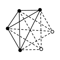
For instance, consider a clique that has neighbours that are connected to focal vertex and therefore vertices that do not have a path of occupied edges to as depicted in Fig 4. There are edges among the vertices in the same component as and interface edges. The bond occupancy probability of this configuration is given by . However, we can remove up to of the occupied edges from the component that belongs to and still retain connectivity among the vertices. Therefore, indexing the number of removed edges by we have
| (48) |
where is the number of connected graphs that can be made that have vertices and edges, see Appendix A. Inserting Eqs 46 and 48 into Eq 44 we arrive at the main result of this section
| (49) |
where . Unpacking this expression when is a 3-clique reproduces Eq 30. When is a 4-clique we obtain
| (50) |
The coefficients of larger cliques are in agreement with the exact expressions previously found by PhysRevE.68.026121 and PhysRevE.104.024304 . The derivative of Eq 49 that is required for the calculation of the finite components is given by
| (51) |
where we can apply Eq 14 to find
| (52) |
The fixed point of these expressions can be found to yield the derivatives and Eq 13 can be solved.
IV Relation to the generalised configuration model
The message passing formulation calculates the properties of a given graph realisation . Often, the properties of an ensemble of networks with equivalent statistics are required, rather than a single instance. An ensemble of random networks can be created according to the generalised configuration model algorithm karrer_newman_2010 ; PhysRevLett.103.058701 ; PhysRevE.80.020901 ; PhysRevE.103.012313 ; PhysRevE.103.012309 . In this model, a set of motifs are defined and each vertex is assigned a tuple of integers, called its joint degree that represents the number of edge-disjoint motifs of a given topology that it belongs to. For instance, if a vertex belongs to three ordinary edges, one triangle, one 4-cycle and two 5-cycles the joint degree is . The distribution of joint degrees are fixed by the joint degree distribution which is the fraction of vertices with a given joint degree.
During the construction process, the configuration model randomises the identity of the vertices that belong to a given motif. Therefore, for a given vertex , the joint degree of its neighbours can vary drastically and so the neighbourhood beyond the nearest neighbours becomes a mean field quantity. To see this, consider an edge-disjoint triangle cover of a network; ordinary edges being present also. All of the edges in the graph have been assigned to a motif topology by the cover that relates to the type of motif to which they belong. Let us now break each edge into two parts whilst retaining the topology labels; isolating each vertex. To create the required number of ordinary edges and triangles, the configuration model selects vertices at random and connects their stubs together, matching the topologies. For instance, to create a triangle, three vertices are selected at random that have free unmatched triangle stubs and are then connected together appropriately. In this way, each random graph that is constructed by the configuration model belongs to an equivalent set of motif topologies, but the identity of the vertices that comprise those motifs will be different. Representing this stochasticity by an average over all graphs in the ensemble, the product of the average message that vertex receives from each of its other motifs can be written as an average over the product of messages
| (53) |
where we have used a version of the Chebyshev integral inequality PhysRevE.82.016101 for monotonic functions of the same monotonicity
| (54) |
In general, the average of a product is not equal to the product of the average. Only when the covariance between the messages is zero is this true. For any two motifs to be correlated in the cavity graph, there must be loops in the factor graph. However, in the limit that the number of vertices becomes infinite, the shortest short range cycles are expected to be at least length . Assuming that the factor graph is locally treelike, then the messages that arrive at a cavity from independent motifs can be treated as though they are uncorrelated with one another; in this case Eq 53 becomes an equality.
As an example, let us partition the product over the motifs of the neighbour into a product over its motif topologies. For instance, for ordinary edges and triangles we have
| (55) |
and
| (56) |
where is the set of ordinary edges (triangles) to which vertex belongs. There are two expressions since motif could have been an ordinary edge or a triangle and the probabilities associated with each one are not equivalent in general. However, since the average message is the same for each motif of a given topology, we can simplify this as a power
| (57) |
where is the excess number of ordinary edges that has (given that is an ordinary edge) and is the number of triangles belongs to. In other words, and . Similarly, if had instead been a triangle we can write
| (58) |
where is the number of ordinary edges and is the excess triangle degree of vertex , respectively. This expression is the product of the average messages along ordinary edges and triangles. The excess degree distributions are distributed as and so averaging over the distribution we can write a generating function for the message that a neighbour receives in the random graph ensemble as
| (59) |
An equivalent argument can be followed to define another fundamental generating function from Eq 10. This logic can be extended to all motifs that are included in the model. With these two generating functions defined, the mapping between the message passing formulation and the generalised configuration model is complete.
V Discussion
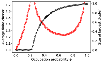
The exact expressions we have derived work well for random graph models, such as the generalised configuration model karrer_newman_2010 ; PhysRevE.103.012309 ; PhysRevE.103.012313 . In Fig 5 we apply these equations to a random graph model comprising 2-, 3- and 4-cliques that has been constructed according to the GCM algorithm; observing excellent agreement between Monte Carlo bond percolation and our theoretical model.
In order to apply our expressions to the study of real world networks, we must find a way to cover the network in motifs. In what amounts to community detection fortunato_hric_2016 , there are perhaps a near infinite number of ways to cover a network with motifs; and some will inherently lead to better models of the empirical network than others 10.5555/1036843.1036914 ; burgio_arenas_gomez_matamalas_2021 ; PhysRevE.105.044314 . The problem of network dismantling is closely related ritmeester_meyer-ortmanns_2022 ; li_2021 ; PhysRevE.103.L061302 .
A trivial solution is to simply cover the network in 2-cliques. In doing this, we are assuming that the network is treelike; this would lead to the traditional belief propagation model, which is known to suffer from statistical errors. To progress beyond this model, the simplest loop we might add to a cover is a triangle; and beyond this chordless cycles and cliques of all orders. However, restricting the permissible motifs to cliques and cycles is unlikely to lead to a locally treelike factor graph. At the other extreme of this logic, one might try to define motifs that contain vertices; perhaps the largest Eulerian cycle for instance. Whilst this cover might lead to a treelike factor graph, we could not hope to write the message passing equations in closed form. Therefore, we must find a balance between motifs that are arbitrary enough to make the factor graph sufficiently treelike, yet are small enough to be analytically tractable such that their message passing equations can be calculated in reasonable time.
Let us suppose that we have defined a set of motifs, perhaps cliques of all sizes. We now have to decide a strategy of how to place the motifs on the network. By far the most simple strategy is to simply search for the presence of a pre-defined set of higher-order motifs and greedily add them to the network cover. This approach is usually stochastic if different starting locations (and subsequent search patterns) are chosen. Burgio et al burgio_arenas_gomez_matamalas_2021 suggest that a maximal cover is the best strategy to retain as much higher-order structure of the empirical networks as possible. In their heuristic, the cover is chosen such that the fewest cliques possible are placed on the network; minimising the local disruption caused by placing a motif. Mann et al PhysRevE.105.044314 showed that preferentially including the largest cliques can be beneficial for retaining the degree correlations among the more well-connected vertices; although this approach is often not maximal. Both of these methods can be generalised to placing motifs other than cliques.
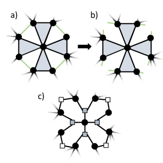
Finally, we would like to highlight another concern that should be accounted for when choosing the motif cover - symmetry. Consider the neighbourhood of a vertex that has been covered by 2- and 3-cliques in Fig 6 a). Due to the edge-disjoint property of the cover, only half of the edges between the neighbours are included in triangles (and therefore, motifs surrounding the focal vertex). When calculating the message passing equations, the focal vertex only observes the effective neighbourhood depicted in Fig 6 b). Because of the asymmetry in how the edges between 1st-order neighbours are accounted for, this cover introduces a statistical bias due to the preferential inclusion of only some of the edges between the 1st-order neighbours and not others. To remove the bias we must either choose the 2-clique cover or, choose the entire motif to be part of the cover. This means that clique covers, which almost always involve breaking symmetry between the neighbours, are inferior to covering methods that account for the entire neighbourhood of a vertex cantwell_newman_2019 .
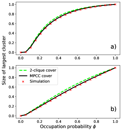
Despite these drawbacks, our model gives good results for real world networks, see Fig 7. In Fig 7 a), we show the size of the largest connected component for a social network of coauthorship relations between 13,861 scientists doi:10.1073/pnas.98.2.404 in the field of condensed-matter physics; and b) a network of 10,680 users of the PGP encryption software PhysRevE.70.056122 . These networks are known to contain a high-density of short loops; and therefore, the standard message passing equations, based on a 2-clique cover (dashed green), fail to correctly predict the size of the percolating cluster. To cover the networks in cliques, we use the so-called motif preserving clique cover (MPCC) PhysRevE.105.044314 . This heuristic attempts to include the largest cliques in the edge-disjoint cover in order to preserve as many contacts among the vertices within a given motif. We find a significant improvement over the 2-clique cover, therefore highlighting the importance of retaining neighbourhood structure for the message passing theory. These networks were previously studied by Cantwell and Newman cantwell_newman_2019 . Their neighbourhood method offers closer agreement to the simulated network than our approach due to the arbitrary nature of the motifs that are included in the cover. It is, however, encouraging that simply incorporating larger cliques into the model offers an improvement over the traditional message passing theory. Cliques are particularly favourable due to the wide range of algorithms and theoretical results that have been developed for these motifs, including those of section III. We comment that finding the clique cover and solving the message passing equations for these networks takes just over 1 minute on 16 GB Apple M1 Silicone, which is very fast compared to other techniques.
VI Conclusion
Belief propagation on loopy networks is a topic that has received much attention in the literature. In this paper, we have studied a bond percolation model on networks that contain simple cycles and cliques by deriving a message passing model. We assume that the factor graph of these networks is locally treelike in order to reduce the correlations between the messages each vertex observes. We examined our theoretical framework for random graphs constructed according to the generalised configuration model as well as a covered empirical networks. We found excellent agreement between Monte Carlo simulation of the average cluster size distribution and the expected size of the percolating component and our equations. Our model offers significant advantage over the traditional belief propagation framework when applied to empirical networks that contain a non-trivial density of loops.
The choice of motif cover is influential to the success of the model and we highlighted some considerations around this. We conjecture that, if the set of motifs that defined the cover in our model was broad or arbitrary enough to capture the local neighbourhood of each vertex at sufficient distance, then our method would produce equivalent results to those of cantwell_newman_2019 . However, it is non-trivial to derive the conditional message probabilities for a given edge configuration of each motif in a closed form expression. Further investigation of the impact of cover choice should be conducted including: the choice of permissible motifs in the model, different cover rules for mesoscale network structures, placing large or small motifs preferentially, the hardness of the constraints in the search for the optimally treelike factor graph and constraints to find optimally symmetric neighbourhood covers.
Finally, we showed how this message passing formulation reproduces the generalised configuration model karrer_newman_2010 when it is averaged over all networks in an ensemble of graphs that have an equivalent joint degree distribution.
These results give important insight into how the belief propagation algorithm can be applied to random and empirical networks. Further work should be carried out to find the critical point of models that contain chordless cycles and cliques PhysRevLett.113.208701 ; PhysRevLett.113.208702 .
Appendix A Number of connected graphs
The number of connected graphs with vertices and edges has been discussed previously in the context of evaluating the percolation formulas for cliques PhysRevE.68.026121 ; PhysRevE.104.024304 . There are at least three well-known approaches to evaluating this quantity including an asymptotic expansion by Flajolet et al flajolet_salvy_schaeffer_2004 , a closed-form expression PhysRevE.104.024304 and a fast recursive formula harary_palmer_1973 due to Harary and Palmer. The recursion is given by
| (60) |
where
| (61) |
This recursive formula can yield the coefficients of cliques with size larger than 100 vertices in fractions of a second running on 16 GB Apple M1 Silicone using Python 3.10.
Appendix B ACKNOWLEDGMENTS
This work was partially supported by the UK Engineering and Physical Sciences Research Council under grant number EP/N007565/1 (Science of Sensor Systems Software).
References
References
- (1) J. Yedidia, W. Freeman, and Y. Weiss, “Constructing free-energy approximations and generalized belief propagation algorithms,” IEEE Transactions on Information Theory, vol. 51, no. 7, p. 2282–2312, 2005.
- (2) M. E. Newman, Networks. Oxford University Press, 2019.
- (3) G. T. Cantwell and M. E. Newman, “Message passing on networks with loops,” Proceedings of the National Academy of Sciences, vol. 116, no. 47, p. 23398–23403, 2019.
- (4) A. Kirkley, G. T. Cantwell, and M. E. Newman, “Belief propagation for networks with loops,” Science Advances, vol. 7, no. 17, 2021.
- (5) M. Mezard, G. Parisi, and R. Zecchina, “Analytic and algorithmic solution of random satisfiability problems,” Science, vol. 297, no. 5582, p. 812–815, 2002.
- (6) R. Monasson and R. Zecchina, “Statistical mechanics of the random -satisfiability model,” Phys. Rev. E, vol. 56, pp. 1357–1370, Aug 1997.
- (7) M. Bronstein, “Beyond message passing: a physics-inspired paradigm for graph neural networks,” The Gradient, 2022.
- (8) C. Bodnar, F. Frasca, Y. Wang, N. Otter, G. F. Montufar, P. Lio, and M. Bronstein, “Weisfeiler and lehman go topological: Message passing simplicial networks,” in International Conference on Machine Learning, pp. 1026–1037, PMLR, 2021.
- (9) H. A. Bethe, “Statistical theory of superlattices,” Proceedings of the Royal Society of London. Series A - Mathematical and Physical Sciences, vol. 150, no. 871, p. 552–575, 1935.
- (10) D. Straszak and N. K. Vishnoi, “Belief propagation, bethe approximation and polynomials,” in 2017 55th Annual Allerton Conference on Communication, Control, and Computing (Allerton), pp. 666–671, Oct 2017.
- (11) A. Weller, K. Tang, D. Sontag, and T. Jebara, “Understanding the bethe approximation: When and how can it go wrong?,” in Proceedings of the Thirtieth Conference on Uncertainty in Artificial Intelligence (UAI-14), 2014.
- (12) B. Karrer, M. E. J. Newman, and L. Zdeborová, “Percolation on sparse networks,” Phys. Rev. Lett., vol. 113, p. 208702, Nov 2014.
- (13) P. D. Gujrati, “Role of loop activity in correlated percolation: results on a husimi cactus and relationship with a bethe lattice,” Journal of Physics A: Mathematical and General, vol. 34, pp. 9211–9230, oct 2001.
- (14) M. Eckstein, M. Kollar, K. Byczuk, and D. Vollhardt, “Hopping on the bethe lattice: Exact results for densities of states and dynamical mean-field theory,” Phys. Rev. B, vol. 71, p. 235119, Jun 2005.
- (15) Y. Shiraki and Y. Kabashima, “Cavity analysis on the robustness of random networks against targeted attacks: Influences of degree-degree correlations,” Phys. Rev. E, vol. 82, p. 036101, Sep 2010.
- (16) F. L. Metz, I. Neri, and D. Bollé, “Spectra of sparse regular graphs with loops,” Phys. Rev. E, vol. 84, p. 055101, Nov 2011.
- (17) S. Yoon, A. V. Goltsev, S. N. Dorogovtsev, and J. F. F. Mendes, “Belief-propagation algorithm and the ising model on networks with arbitrary distributions of motifs,” Phys. Rev. E, vol. 84, p. 041144, Oct 2011.
- (18) M. E. J. Newman, “Spectra of networks containing short loops,” Phys. Rev. E, vol. 100, p. 012314, Jul 2019.
- (19) K. E. Hamilton and L. P. Pryadko, “Tight lower bound for percolation threshold on an infinite graph,” Phys. Rev. Lett., vol. 113, p. 208701, Nov 2014.
- (20) A. Coolen, “Replica methods for loopy sparse random graphs,” Journal of Physics: Conference Series, vol. 699, p. 012022, mar 2016.
- (21) B. J. Frey and D. MacKay, “A revolution: Belief propagation in graphs with cycles,” in Advances in Neural Information Processing Systems (M. Jordan, M. Kearns, and S. Solla, eds.), vol. 10, MIT Press, 1997.
- (22) M. E. J. Newman, X. Zhang, and R. R. Nadakuditi, “Spectra of random networks with arbitrary degrees,” Phys. Rev. E, vol. 99, p. 042309, Apr 2019.
- (23) M. Chertkov and V. Y. Chernyak, “Loop calculus in statistical physics and information science,” Phys. Rev. E, vol. 73, p. 065102, Jun 2006.
- (24) M. E. J. Newman, “Random graphs with clustering,” Phys. Rev. Lett., vol. 103, p. 058701, Jul 2009.
- (25) J. C. Miller, “Percolation and epidemics in random clustered networks,” Phys. Rev. E, vol. 80, p. 020901, Aug 2009.
- (26) B. Karrer and M. E. J. Newman, “Random graphs containing arbitrary distributions of subgraphs,” Physical Review E, vol. 82, no. 6, 2010.
- (27) T. Hasegawa and S. Mizutaka, “Structure of percolating clusters in random clustered networks,” Phys. Rev. E, vol. 101, p. 062310, Jun 2020.
- (28) P. Mann, V. A. Smith, J. B. O. Mitchell, and S. Dobson, “Degree correlations in graphs with clique clustering,” Phys. Rev. E, vol. 105, p. 044314, Apr 2022.
- (29) P. Mann, V. A. Smith, J. B. O. Mitchell, C. Jefferson, and S. Dobson, “Exact formula for bond percolation on cliques,” Phys. Rev. E, vol. 104, p. 024304, Aug 2021.
- (30) P. Mann, V. A. Smith, J. B. O. Mitchell, and S. Dobson, “Percolation in random graphs with higher-order clustering,” Phys. Rev. E, vol. 103, p. 012313, Jan 2021.
- (31) P. Mann, V. A. Smith, J. B. O. Mitchell, and S. Dobson, “Random graphs with arbitrary clustering and their applications,” Phys. Rev. E, vol. 103, p. 012309, Jan 2021.
- (32) G. Burgio, A. Arenas, S. Gomez, and J. T. Matamalas, “Network clique cover approximation to analyze complex contagions through group interactions,” Communications Physics, vol. 4, no. 1, 2021.
- (33) T. Hasegawa and Y. Iwase, “Observability transitions in clustered networks,” Physica A: Statistical Mechanics and its Applications, vol. 573, p. 125970, 2021.
- (34) This is certainly not true for motifs whose vertices do not belong to the same site (or more correctly - orbit). In that case, the bond occupancy probability depends on the identity of the vertices in the connected component (see PhysRevE.104.024304 ).
- (35) M. E. J. Newman, “Properties of highly clustered networks,” Phys. Rev. E, vol. 68, p. 026121, Aug 2003.
- (36) B. Karrer and M. E. J. Newman, “Message passing approach for general epidemic models,” Phys. Rev. E, vol. 82, p. 016101, Jul 2010.
- (37) S. Fortunato and D. Hric, “Community detection in networks: A user guide,” Physics Reports, vol. 659, p. 1–44, 2016.
- (38) M. Welling, “On the choice of regions for generalized belief propagation,” in Proceedings of the 20th Conference on Uncertainty in Artificial Intelligence, UAI ’04, (Arlington, Virginia, USA), p. 585–592, AUAI Press, 2004.
- (39) T. Ritmeester and H. Meyer-Ortmanns, “Belief propagation for supply networks: Efficient clustering of their factor graphs,” The European Physical Journal B, vol. 95, no. 5, 2022.
- (40) T. Li, “Network dismantling on factor graphs: Break long loops and spare local structures,” New Journal of Physics, vol. 23, no. 10, p. 103014, 2021.
- (41) T. Li, P. Zhang, and H.-J. Zhou, “Long-loop feedback vertex set and dismantling on bipartite factor graphs,” Phys. Rev. E, vol. 103, p. L061302, Jun 2021.
- (42) M. E. J. Newman, “The structure of scientific collaboration networks,” Proceedings of the National Academy of Sciences, vol. 98, no. 2, pp. 404–409, 2001.
- (43) M. Boguñá, R. Pastor-Satorras, A. Díaz-Guilera, and A. Arenas, “Models of social networks based on social distance attachment,” Phys. Rev. E, vol. 70, p. 056122, Nov 2004.
- (44) P. Flajolet, B. Salvy, and G. Schaeffer, “Airy phenomena and analytic combinatorics of connected graphs,” The Electronic Journal of Combinatorics, vol. 11, no. 1, 2004.
- (45) F. Harary and E. M. Palmer, Graphical enumeration. Academic Press, 1973.