Weighted trace-penalty minimization for full configuration interaction

Abstract

A novel unconstrained optimization model named weighted trace-penalty minimization (WTPM) is proposed to address the extreme eigenvalue problem arising from the Full Configuration Interaction (FCI) method. Theoretical analysis shows that the global minimizers of the WTPM objective function are the desired eigenvectors, rather than the eigenspace. Analyzing the condition number of the Hessian operator in detail contributes to the determination of a near-optimal weight matrix. With the sparse feature of FCI matrices in mind, the coordinate descent (CD) method is adapted to WTPM and results in WTPM-CD method. The reduction of computational and storage costs in each iteration shows the efficiency of the proposed algorithm. Finally, the numerical experiments demonstrate the capability to address large-scale FCI matrices.

65F15

1 Introduction

The time-independent, non-relativistic Schrödinger equation is a linear Hermitian extreme eigenvalue problem,

(1.1) $$H\ket{\psi_{i}}=E_{i}\ket{\psi_{i}},\quad i=1,2,\dots,p,$$

where $H$ is a Hamiltonian operator, $(E_{i},\ket{\psi_{i}})$ denotes the ground-state and lowest few excited-state energies and their corresponding wavefunctions, and $p$ is the number of desired eigenvalues. Efficiently solving the Schrödinger equation plays a fundamental role in the field of electronic structure calculation. The problem is of high-dimensionality, i.e., $\ket{\psi}=\psi(x_{1},\dots,x_{N_{\mathrm{e}}})$ for $x_{i}\in\mathbb{R}^{3}$ being the position of electrons and ${N_{\mathrm{e}}}$ being the number of active electrons in the system. Further, identical electron wavefunctions admit an antisymmetry property, which corresponds to the Pauli exclusion principle. Full configuration interaction (FCI) is a variational method that solves (1.1) numerically exactly within the space of all Slater determinants [21, 22, 38]. By the nature of Slater determinants, the antisymmetry property is encoded into the many-body basis functions. Nevertheless, the high-dimensionality feature still leads to extremely large Hamiltonian matrices. More precisely, the size of Hamiltonian matrices grows factorially with respect to the number of electrons and orbitals in the system. For a system with ${N_{\mathrm{orb}}}$ orbitals and ${N_{\mathrm{e}}}$ electrons, the number of Slater determinants is $O\Big{(}\tbinom{{N_{\mathrm{orb}}}}{{N_{\mathrm{e}}}}\Big{)}$ [23]. A single $\ch{H2O}$ molecule with cc-pVDZ basis ($24$ orbitals) and 10 active electrons leads to a $4.53\cdot 10^{8}\times 4.53\cdot 10^{8}$ Hamiltonian matrix [43]. The antisymmetry property of the problems leads to the notorious sign problem.

In electronic structure calculation, widely used eigensolvers can be classified into two groups: Krylov subspace methods and optimization methods. Krylov subspace methods include Chebyshev-Davidson algorithm [47], locally optimal block preconditioned conjugate gradient method (LOBPCG) [24], block Krylov-Schur algorithm [48], projected preconditioned conjugate gradient algorithm (PPCG) [42], etc. In all these methods, an explicit orthogonalization step is carried out every few iterations, which costs a significant amount of computational resource throughout the algorithm. The other group, optimization methods, transforms the eigenvalue problem into an optimization problem with or without the orthogonality constraint. The orthogonality constrained optimization problem is also known as the Stiefel manifold optimization. The corresponding optimization algorithms [1, 14, 19, 36] require either a projection or a retraction step to keep the iteration on the manifold. The computational costs for these projections and retractions remain the same as that of the orthogonalization. Solving the eigenvalue problem via an unconstrained optimization is popular recently, especially when the large-scale eigenvalue problems are considered. Such methods include symmetric low-rank product model [27, 29, 43], orbital minimization method (OMM) [13, 30], trace-penalty minimization [45], etc. All these methods converge to the invariant subspace corresponding to the smallest eigenvalues, and require a single Rayleigh-Ritz procedure to extract eigenvectors from the invariant subspace.

However, due to the large-scale matrix size, none of the eigensolvers mentioned above can be applied directly to the FCI eigenvalue problem. Almost all of them run into the memory bottleneck. Many non-standard eigensolvers are designed particularly for FCI ground-state computation. Density matrix renormalization group (DMRG) [9, 33, 46] approximates the high-dimensional wavefunctions by a tensor train. The underlying eigenvalue problem is solved by the vanilla power method. FCI quantum Monte Carlo (FCIQMC) [6, 7, 31] adopts the quantum Monte Carlo method to overcome the sign problem and the curse of dimensionality. Related methods [11, 35] in this family further adjust the variance-bias trade-off to obtain efficient algorithms. Selected configuration interaction (SCI) [18, 20, 37, 41] employs perturbation analysis of eigenvalue problems and selects important configurations accordingly. Then the eigenvalue problem of the selected principal submatrix is solved via traditional eigensolvers. Various methods in this family differ from each other in the computationally efficient approximations to the perturbation result. Coordinate descent FCI (CDFCI) [27, 43] applies the coordinate descent method on the symmetric low-rank product model to select important configurations and to update the coefficients. A carefully designed compression scheme is incorporated to overcome the memory bottleneck.

Furthermore, the non-standard eigensolvers mentioned above can be adapted to the low-lying excited-states computation. DMRG [2] and FCIQMC [5] adopt the deflation idea and compute excited-states one-by-one. SCI [37, 41] needs to select many more configurations to capture the important configurations for excited states. CDFCI [44] could be naturally extended and converge to the invariant subspace formed by the ground-state and excited-states. The extra rotation matrix within the invariant subspace leads to less sparse iteration variables and increases the memory cost. Specifically targeting the low-lying excited-states computation, the triangularized orthogonalization free method (TriOFM) [15, 16] proposes a triangularized iterative scheme converging to eigenvectors directly without any projection or Rayleigh-Ritz step.

In this paper, inspired by the weighted subspace-search variational quantum eigensolver [32] from quantum computing and the trace-penalty model [45], we propose an unconstrained optimization model called weighted trace-penalty minimization (WTPM),

(1.2) $$\min_{X\in\mathbb{R}^{n\times p}}f_{\mu,W}(X)=\frac{1}{2}\mathrm{tr}(X^{\top}AX)+\frac{\mu}{4}\norm{X^{\top}X-W}_{\mathrm{F}}^{2},$$

where $A\in\mathbb{R}^{n\times n}$ is a symmetric matrix, $\mu>0$ is the penalty parameter and $W$ is a diagonal weight matrix with distinct diagonal entries. Our analysis shows that (1.2) does not have spurious local minima, and the $2^{p}$ isolated global minima of (1.2) are scaled eigenvectors corresponding to the smallest $p$ eigenvalues of $A$. Moreover, we calculate the condition number of the $W$-dependent Hessian matrix of $f_{\mu,W}(X)$ at global minima, which leads to the local convergence rate for the first-order method. A near-optimal weight matrix $W$ is, then, derived to achieve a fast local convergence rate.

With the size of FCI problem size in mind, we focus on first-order methods to address (1.2). One choice is the gradient descent (GD) method with Barzilai-Borwein (BB) stepsize [3]. A more desirable choice is the coordinate descent (CD) method, which reveals the sparsity in FCI problems efficiently [43]. Hence, we tailor the CD method for (1.2) and obtain an efficient eigensolver for the FCI eigenvalue problem. Global convergence of the proposed eigensolver can be proved in the same way as that of CDFCI [27], whereas the local linear convergence is obtained with a rate related to the Hessian operator. We emphasize that both GD and CD methods for (1.2) converge to the scaled eigenvectors directly. Hence the expensive and parallel inefficient Rayleigh-Ritz step is omitted entirely from both methods.

Numerically, we test and compare the performance of the original trace-penalty model [45] and our WTPM on FCI matrices from practice. The numerical results show that both models with first-order methods converge to desired global minima. Adding the extra weight matrix in WTPM does not destroy the efficiency of the original trace-penalty model. For the FCI matrices, WTPM-CD method converges in far less cost of flops. WTPM-CD finds the sparse representations of the eigenvectors corresponding to the smallest few eigenvalues, whereas the trace-penalty model requires an extra Rayleigh-Ritz step.

The rest of this paper is organized as follows. In Section 2, we give a theoretical analysis on (1.2) with a focus on the global minima and the condition number of the Hessian operator. Section 3 proposes algorithms for (1.2) and analyzes their performance and complexity. Section 4 reports the numerical results showing the efficiency of our method. Finally, we conclude this paper in Section 5 with some discussion on future work.

2 Model Analysis

This section focuses on the analysis of the energy landscape of the weighted trace-penalty minimization model. We will first analyze the stationary points and Hessian operator of (1.2) in Section 2.1 and Section 2.2 respectively. Based on the condition number of the Hessian operator at the global minimum, a near-optimal choice of the weight matrix $W$ is discussed in Section 2.3 to achieve a near-optimal local convergence rate for first-order methods. Finally in Section 2.4, we discuss the extensions of all analysis results to Hermitian matrices.

We consider a real symmetric matrix $A$ of size $n\times n$. The eigenvalue decomposition of $A$ is denoted as,

(2.1) $$A=V\Lambda V^{\top},$$

where $V=(v_{1},v_{2},\dots,v_{n})\in\mathbb{R}^{n\times n}$ and $\Lambda=\mathrm{diag}(\lambda_{1},\lambda_{2},\dots,\lambda_{n})$ such that

(2.2) $$\lambda_{1}<\lambda_{2}<\cdots<\lambda_{p}<\lambda_{p+1}\leqslant\cdots\leqslant\lambda_{n}.$$

A pair $(\lambda_{i},v_{i})$ is an eigenpair of $A$. Throughout this paper, we aim to compute the smallest $p$ eigenpairs of $A$ via WTPM. The real weight matrix in (1.2) satisfies the following assumption.

Assumption 1.

The weight matrix is diagonal, $W=\mathrm{diag}(w_{1},w_{2},\dots,w_{p})$ such that

(2.3) $$w_{1}>w_{2}>\cdots>w_{p}>\frac{\lambda_{p}}{\mu}.$$

2.1 Stationary Points

Stationary points of (1.2) satisfy the first-order necessary optimal condition,

(2.4) $$\nabla f_{\mu,W}(X)=AX+\mu X(X^{\top}X-W)=0.$$

Left multiplying both sides of (2.4) by the transpose of $X$, we obtain,

(2.5) $$X^{\top}AX=\mu X^{\top}X(W-X^{\top}X),$$

where the left-hand side is symmetric. The symmetry property of (2.5) leads to the fact that $X^{\top}XW=WX^{\top}X$. Since $W$ is a diagonal matrix and all entries are distinct as in (2.3), the equation $X^{\top}XW=WX^{\top}X$ implies that $X^{\top}X$ is diagonal, i.e., columns of stationary point $X$ are either zero or mutually orthogonal. In Theorem 2.1, we give the explicit form of the stationary points of (1.2), where each column of $X$ is either an eigenvector of $A$ or the zero vector.

Theorem 2.1 (Stationary Points).

Assume $A$ and $W$ satisfy (2.1) and (2.3) respectively. Any stationary point $\widehat{X}$ of (1.2) has the form

(2.6) $$\widehat{X}=\widehat{U}_{p}\widehat{S}_{p},$$

where $\widehat{U}_{p}=(\hat{u}_{1},\hat{u}_{2},\dots,\hat{u}_{p})$ and $\widehat{S}_{p}=\mathrm{diag}(\hat{s}_{1},\hat{s}_{2},\dots,\hat{s}_{p})$ such that

(2.7) $$\begin{split}A\hat{u}_{i}=\sigma_{i}\hat{u}_{i},\quad\hat{u}_{i}^{\top}\hat{u}_{j}=\delta_{ij}\text{ and,}\\ \hat{s}_{i}\in\left\{0,\sqrt{w_{i}-\frac{\sigma_{i}}{\mu}}\right\}.\end{split}$$

Proof 2.2.

As we discussed above, $\widehat{X}^{\top}\widehat{X}$ is a diagonal matrix. Columns of (2.4), then, can be represented as

(2.8) $$A\hat{x}_{i}=d_{i}\hat{x}_{i},\quad i=1,2,\dots,p,$$

where $\hat{x}_{i}$ is the $i$-th column of $\widehat{X}$ and $d_{i}=\mu(w_{i}-\hat{x}^{\top}_{i}\hat{x}_{i})$. Vector $\hat{x}_{i}$ is either a zero vector or an eigenvector of $A$. When $\hat{x}_{i}$ is a zero vector, it can be represented as the form in the theorem for $\hat{s}_{i}=0$. When $\hat{x}_{i}$ is not a zero vector, we denote $\hat{x}_{i}=\hat{u}_{i}\hat{s}_{i}$ for $\hat{u}_{i}$ being a unit length eigenvector of $A$ associated with eigenvalue $\sigma_{i}$ and $\hat{s}_{i}$ being a positive scalar. Then $\hat{s}_{i}$ satisfies

$$\sigma_{i}=d_{i}=\mu(w_{i}-\hat{s}_{i}^{2})\Rightarrow\hat{s}_{i}=\sqrt{w_{i}-\frac{\sigma_{i}}{\mu}}.$$

Recall that $\widehat{X}^{\top}\widehat{X}$ is a diagonal matrix. For nonzero $\hat{s}_{i}$ and $\hat{s}_{j}$, it is required that $\hat{u}_{i}^{\top}\hat{u}_{j}=\delta_{ij}$. When $\hat{s}_{i}$ is zero, we could always find an extra orthogonal eigenvector of $A$, such that $\hat{u}_{i}^{\top}\hat{u}_{j}=\delta_{ij}$ still holds. Therefore, we proved that the stationary points of (1.2) must admit the form in the theorem and any point that admits the form in the theorem is a stationary point.

Furthermore, we will distinguish the local and global minima from saddle points. Interestingly, it can be shown that the columns of global minimizer $X^{*}$ are eigenvectors of $A$ associated with the $p$ smallest eigenvalues.

Theorem 2.3 (Global Minima).

Assume $A$ and $W$ satisfy (2.1) and (2.3). Any global minimizer $X^{*}$ of (1.2) has the form

(2.9) $$X^{*}=V_{p}S_{p},$$

where $V_{p}=(v_{1},v_{2},\dots,v_{p})$ and $S_{p}=\mathrm{diag}(\pm s_{1},\pm s_{2},\dots,\pm s_{p})$ such that

$$s_{i}=\sqrt{w_{i}-\frac{\lambda_{i}}{\mu}}.$$

Proof 2.4.

By Theorem 2.1, the stationary point has the form $\widehat{X}=\widehat{U}_{p}\widehat{S}_{p}$. Substituting it into the objective function leads to,

$$2f_{\mu,W}(\widehat{X})=\sum_{i=1}^{p}\bigl{[}\hat{s}_{i}^{2}\sigma_{i}+\frac{\mu}{2}(\hat{s}_{i}^{2}-w_{i})^{2}\bigr{]}=\sum_{i=1}^{p}\frac{\mu}{2}w_{i}^{2}-\sum_{i\in\{\hat{s}_{i}\neq 0\}}\frac{(\sigma_{i}-\mu w_{i})^{2}}{2\mu},$$

where $\sigma_{i}$ is one of the eigenvalues of $A$ and the second equality is due to the expression of $\hat{s}_{i}$. If some $\hat{s}_{i}=0$, then we have $\sigma_{i}-\mu w_{i}=0$. Under Assumption 1, there are at least $p$ eigenvalues to make $-\tfrac{(\lambda-\mu w_{i})^{2}}{2\mu}<0$ and at least one of them is not in $\{\sigma_{i}\}_{i=1}^{p}$. Replacing $\sigma_{i}$ by one of the unselected eigenvalue with $-\tfrac{(\lambda-\mu w_{i})^{2}}{2\mu}<0$ would lead to a smaller objective function value. Hence if $\hat{s}_{i}=0$ for some $i$, the stationary point is not a global minimizer. Notice that if $\hat{s}_{i}\neq 0$ then $\sigma_{i}<\mu w_{i}$. We only need to show that $\sigma_{i}=\lambda_{i}$.

First, we claim that $\sigma_{1},\sigma_{2},\dotsc,\sigma_{p}$ must be a permutation of $\lambda_{1},\lambda_{2},\dotsc,\lambda_{p}$. If not, for example there exists $\sigma_{i_{0}}$ such that $\mu w_{i_{0}}>\sigma_{i_{0}}>\lambda_{p}$. There also exists $\lambda_{j}$ not used such that $\lambda_{j}\leqslant\lambda_{p}$. If $\sigma_{i_{0}}=\lambda_{j}$ instead, the value of $f_{\mu,W}(\widehat{X})$ will decrease. This contradicts with the minimal property so our claim holds.

Next, since there are at least $p$ eigenvalues smaller than any $\mu w_{i}$ due to Assumption 1, the optimization (1.2) changes into the form as

(2.10) $$\max_{\begin{subarray}{c}\sigma_{i}\in\{\lambda_{1},\dotsc,\lambda_{p}\}\\ \sigma_{i}\neq\sigma_{j}\;\text{if }i\neq j\end{subarray}}\sum_{i=1}^{p}(\sigma_{i}-\mu w_{i})^{2}=\sum_{i=1}^{p}-2\mu\sigma_{i}w_{i}+\text{const}.$$

According to Rearrangement Inequality [17], we can conclude that the minimum value is reached if $\sigma_{i}=\lambda_{i}$, i.e.

$$X^{*}=V_{p}S_{p}.$$

Theorem 2.3 presents an interesting result that any global minimizer of the WTPM (1.2) is composed of desired eigenvectors directly rather than the underlying invariant subspace.

Another result is that there are no spurious local minima, i.e., the rest stationary points are all strict saddle points. To show this, we first introduce the Hessian operator of $f_{\mu,W}$,

(2.11) $$\mathrm{Hess}\,f_{\mu,W}(X)[Z]=AZ+\mu(ZX^{\top}X+XZ^{\top}X+XX^{\top}Z-ZW),$$

where $Z\in\mathbb{R}^{n\times p}$ is an arbitrary matrix. A stationary point $\hat{X}$ is called a strict saddle point of $f_{\mu,W}$ if and only if the Hessian operator $\mathrm{Hess}\,f_{\mu,W}(\hat{X})$ has negative eigenvalues. 

In Theorem 2.5, we prove that (1.2) does not have any spurious local minimum.

Theorem 2.5.

Assume $A$ and $W$ satisfy (2.1) and (2.3). There are no local minima other than the global minimizers $X^{*}$.

Proof 2.6.

First, we discuss the case that the stationary point $\widehat{X}=\widehat{U}_{p}\widehat{S}_{p}$ is of full column rank, i.e., $\hat{s}_{i}\neq 0,\forall i$. We focus on the sign of

(2.12) $$\mathrm{tr}\left(Z^{\top}\mathrm{Hess}\,f_{\mu,W}(\hat{X})[Z]\right)=\\ \mathrm{tr}\left(Z^{\top}(A+\mu\hat{X}\hat{X}^{\top})Z+\mu Z^{\top}Z(\hat{X}^{\top}\hat{X}-W)+\mu Z^{\top}\hat{X}Z^{\top}\hat{X}\right),$$

for $Z\in\mathbb{R}^{n\times p}$. If (2.12) at $\hat{X}$ is strictly negative for a particular $Z$, then we could conclude that the Hessian operator has negative eigenvalues and hence $\hat{X}$ is a strict saddle point.

Since $\hat{X}$ is not global minimizer, there exists an eigenvector $v_{i}$ in $\{v_{1},v_{2},\dotsc,v_{p}\}$ satisfying $v_{i}^{\top}\hat{U}_{p}=0$ and $\exists j,\;\lambda_{i}<\sigma_{j}$. Let $Z$ be the matrix whose $j$-th column is $v_{i}$ and others are zero. Then we have

(2.13) $$\mathrm{tr}\left(Z^{\top}\mathrm{Hess}\,f_{\mu,W}(\hat{X})[Z]\right)=\lambda_{i}-\sigma_{j}<0,$$

implying that full-rank stationary points are all saddle points except global minima.

Next, we discuss the rank-deficient case. Without loss of generality we assume the $j$-th column of $\hat{X}$ is zero, and there also exists an eigenvector $v_{i}$ in $\{v_{1},v_{2},\dotsc,v_{p}\}$ satisfying $v_{i}^{\top}\hat{X}=0$. Let $j$-th column of $Z$ be $v_{i}$ and others are zero. We can obtain

(2.14) $$\mathrm{tr}\left(Z^{\top}\mathrm{Hess}\,f_{\mu,W}(\hat{X})[Z]\right)=\lambda_{i}-\mu w_{j}<0.$$

Hence, rank-deficient stationary points are all saddle points.

2.2 Hessian Operator

For first-order optimization methods, the local convergence rate relies on the condition number of the Hessian operator [8]. Specifically, in the neighborhood of a global minimum $X^{*}$, the error of a gradient descent method with exact line search decreases linearly as

(2.15) $$f_{\mu,W}(X^{(j+1)})-f_{\mu,W}(X^{*})\leqslant\bigl{(}1-\kappa^{-1}\bigr{)}\bigl{(}f_{\mu,W}(X^{(j)})-f_{\mu,W}(X^{*})\bigr{)}$$

where $X^{(j)}$ denotes the iteration variable at $j$-th iteration and $\kappa$ denotes the condition number of the Hessian operator at $X^{*}$.

From Theorem 2.3, we find that all global minima of (1.2) are isolated points and the Hessian operator at any global minimizer $X^{*}$ is strictly positive definite. In order to give a depiction of the local convergence rate of (1.2), we present a tight estimation of the condition number of the Hessian operator in Theorem 2.7.

Theorem 2.7.

Assume $A$ and $W$ satisfy (2.1) and (2.3). Let $X^{*}$ be a global minimizer of $f_{\mu,W}$. Then

(2.16a) $$\kappa\left(\mathrm{Hess}\,f_{\mu,W}(X^{*})\right) \triangleq\frac{\max\limits_{\norm{Z}_{\mathrm{F}}=1}\mathrm{tr}\left(Z^{\top}\mathrm{Hess}\,f_{\mu,W}(X^{*})[Z]\right)}{\min\limits_{\norm{Z}_{\mathrm{F}}=1}\mathrm{tr}\left(Z^{\top}\mathrm{Hess}\,f_{\mu,W}(X^{*})[Z]\right)},$$

(2.16b) $$=\frac{\max\left\{\lambda_{n}-\lambda_{1},2(\mu w_{1}-\lambda_{1}),\max\limits_{i<j}\lambda_{\max}(M_{ij})\right\}}{\min\left\{\lambda_{p+1}-\lambda_{p},2(\mu w_{p}-\lambda_{p}),\min\limits_{i<j}\lambda_{\min}(M_{ij})\right\}},$$

where $\lambda_{\max}(\cdot)$ and $\lambda_{\min}(\cdot)$ denote the largest and the smallest eigenvalue of the matrix

$$M_{ij}=\begin{pmatrix}\mu w_{i}-\lambda_{j}&\sqrt{(\mu w_{i}-\lambda_{i})(\mu w_{j}-\lambda_{j})}\\ \sqrt{(\mu w_{i}-\lambda_{i})(\mu w_{j}-\lambda_{j})}&\mu w_{j}-\lambda_{i}\end{pmatrix}$$

respectively.

Proof 2.8.

Given a $Z\in\mathbb{R}^{n\times p}$ such that $\norm{Z}_{\mathrm{F}}=1$, it can be represented as

$$Z=V_{p}Z_{1}+\widebar{V}_{p}Z_{2},$$

$$\mathrm{tr}(Z_{1}^{\top}Z_{1})+\mathrm{tr}(Z_{2}^{\top}Z_{2})=1,$$

where $\widebar{V}_{p}=(v_{p+1},\ldots,v_{n})$, $Z_{1}\in\mathbb{R}^{p\times p}$, and $Z_{2}\in\mathbb{R}^{(n-p)\times p}$. Using the expressions of the global minimizer (2.9) and the Hessian operator (2.11), we obtain,

(2.17) $$\mathrm{tr}\left(Z^{\top}\mathrm{Hess}\,f_{\mu,W}(X^{*})[Z]\right)=\mathrm{tr}(Z_{2}^{\top}\widebar{\Lambda}_{p}Z_{2})-\mathrm{tr}(Z_{2}^{\top}Z_{2}\Lambda_{p})\\ +\mathrm{tr}(\mu Z_{1}^{\top}WZ_{1})-\mathrm{tr}(Z_{1}^{\top}Z_{1}\Lambda_{p})+\mathrm{tr}(\mu Z_{1}^{\top}S_{p}Z_{1}^{\top}S_{p}),$$

where $\Lambda_{p}=\mathrm{diag}(\lambda_{1},\ldots,\lambda_{p})$ and $\widebar{\Lambda}_{p}=\mathrm{diag}(\lambda_{p+1},\ldots,\lambda_{n})$. The first two terms in (2.17) can be bounded as,

(2.18) $$\mathrm{tr}(Z_{2}^{\top}Z_{2})(\lambda_{p+1}-\lambda_{p})\leqslant\mathrm{tr}(Z_{2}^{\top}\bar{\Lambda}_{p}Z_{2})-\mathrm{tr}(Z_{2}^{\top}Z_{2}\Lambda_{p})\leqslant\mathrm{tr}(Z_{2}^{\top}Z_{2})(\lambda_{n}-\lambda_{1}),$$

where the upper and lower bounds are achieved when $Z_{2}=c\cdot(e_{n-p},0,\ldots,0)$ or $Z_{2}=c\cdot(0,\ldots,0,e_{1})$, where $e_{i}$ denotes the $i$-th column of the identity matrix and $c$ is a scalar.

Next, we would like to bound the terms in (2.17) associated with $Z_{1}$. Let $Z_{1}=(z_{ij})_{p\times p}$. A short calculation shows that

(2.19) $$\begin{split}&\mathrm{tr}(\mu Z_{1}^{\top}WZ_{1})-\mathrm{tr}(Z_{1}^{\top}Z_{1}\Lambda_{p})+\mu\mathrm{tr}(Z_{1}^{\top}S_{p}Z_{1}^{\top}S_{p})\\ =&2\sum_{i=1}^{p}(\mu w_{i}-\lambda_{i})z_{ii}^{2}+\sum_{j>i}\begin{pmatrix}z_{ij}&z_{ji}\end{pmatrix}M_{ij}\begin{pmatrix}z_{ij}\\ z_{ji}\end{pmatrix},\end{split}$$

where $M_{ij}\in\mathbb{R}^{2\times 2}$ as defined in the theorem. Eigenvalues of $M_{ij}$ can be calculated explicitly,

(2.20) $$\begin{split}\lambda(M_{ij})&=\frac{1}{2}(\mu w_{i}+\mu w_{j}-\lambda_{i}-\lambda_{j})\\ &\pm\sqrt{\frac{1}{4}(\mu w_{i}+\mu w_{j}-\lambda_{i}-\lambda_{j})^{2}-\mu(w_{i}-w_{j})(\lambda_{j}-\lambda_{i})},\end{split}$$

and both of them are positive. Thus, (2.19) has the lower and upper bounds,

(2.21a) $$\eqref{eq:Z1Part} \geqslant\mathrm{tr}(Z_{1}^{\top}Z_{1})\cdot\min\left\{2(\mu w_{p}-\lambda_{p}),\min\limits_{i<j}\lambda_{\min}(M_{ij})\right\},$$

(2.21b) $$\eqref{eq:Z1Part} \leqslant\mathrm{tr}(Z_{1}^{\top}Z_{1})\cdot\max\left\{2(\mu w_{1}-\lambda_{1}),\max\limits_{i<j}\lambda_{\max}(M_{ij})\right\}.$$

Again, both bounds in (2.21) are achievable. In (2.21a), the inequality is saturated if $Z_{1}$ is parallel to $(0,\dotsc,0,e_{p})$, or if $(z_{ij},z_{ji})^{\top}$ is the eigenvector corresponding to $\min_{i<j}\lambda_{\min}(M_{ij})$ and other entries of $Z_{1}$ are zero. Similarly in (2.21b), the equality is satisfied if $Z_{1}$ is parallel to $(e_{1},0,\dotsc,0)$, or if $(z_{ij},z_{ji})^{\top}$ is the eigenvector corresponding to $\max_{i<j}\lambda_{\max}(M_{ij})$ and other entries of $Z_{1}$ are zero. Putting all bounds in (2.18) and (2.21) together, we proved (2.16).

Theorem 2.7 gives the exact condition number at global minimizers, which provides an estimation of the local convergence rate around the optima. Based on (2.16), we could estimate the local convergence if the weight matrix $W$ is chosen. In order to minimize the condition number of Hessian operator, we will provide an intuitive approach to select a near-optimal weight matrix in the next section.

Remark 2.9.

We give a discussion for matrices with degenerate eigenvalues among $\lambda_{1},\lambda_{2},\dots,\lambda_{p}$, i.e., we relax the assumption (2.2) as

(2.22) $$\lambda_{1}\leqslant\lambda_{2}\leqslant\cdots\leqslant\lambda_{p}<\lambda_{p+1}\leqslant\cdots\leqslant\lambda_{n}.$$

Theorem 2.1 and Theorem 2.5 remains valid in their current forms. Theorem 2.3 is also valid up to some changes due to the non-uniqueness of the eigenvectors of $A$. We give an example to show the idea of the required changes. Assume $\lambda_{i}=\lambda_{i+1}$ for $i<p$. Then any vector $v\in\mathrm{span}\{v_{i},v_{i+1}\}$ is an eigenvector of $A$ corresponding to $\lambda_{i}$ and $\lambda_{i+1}$. Therefore, the matrix $V_{p}$ in Theorem 2.3 may not be in the current form, $V=(v_{1},v_{2},\dotsc,v_{n})$. Instead, the matrix $V_{p}$ could be changed to

$$V_{p}=(v_{1},v_{2},\dotsc,v_{p})\cdot\begin{pmatrix}I_{i-1}&&\\ &Q_{1}&\\ &&I_{n-i-1}\end{pmatrix},$$

where $Q_{1}$ is a $2\times 2$ orthogonal matrix. More generally, if there are $r$ distinct eigenvalues among $\{\lambda_{1},\lambda_{2},\dotsc,\lambda_{p}\}$, the matrix $V_{p}$ in Theorem 2.3 admits the form

$$V_{p}=(v_{1},v_{2},\dotsc,v_{p})\cdot\begin{pmatrix}Q_{1}&&&\\ &Q_{2}&&\\ &&\ddots&\\ &&&Q_{r}\end{pmatrix},$$

where $Q_{i}$ is an orthogonal matrix with dimension being the degree of degeneracy of the $i$th distinct eigenvalues.

However, as for Theorem 2.7, since the global minimizers are not isolated, the Hessian matrix of $f_{\mu,W}$ at $X^{*}$ cannot be positive definite. We could employ techniques in Section 2.4 to remove the nonzero null space in the Hessian matrix.

2.3 Near-Optimal Weight Matrix

According to the analysis above, the parameter $\mu$ and the weight matrix $W$ could be considered as an ensemble $\mu W$. That means that the degree of freedom of the parameters in (1.2) is $p$ instead of $p+1$. Therefore, we can always set that $\mu=1$ in analysis. Given the exact expression of the condition number $\kappa\left(\mathrm{Hess}\,f_{\mu,W}(X^{*})\right)$, we would like to minimize the condition number with respect to the weight matrix $W$ and obtain the optimal weight matrix $W^{*}$, i.e.,

(2.23) $$W^{*}=\mathop{\arg\min}_{W}\frac{\max\left\{\lambda_{n}-\lambda_{1},2(w_{1}-\lambda_{1}),\max\limits_{i<j}\lambda_{\max}(M_{ij})\right\}}{\min\left\{\lambda_{p+1}-\lambda_{p},2(w_{p}-\lambda_{p}),\min\limits_{i<j}\lambda_{\min}(M_{ij})\right\}}.$$

However, (2.23) relies on the eigenvalues of $A$, which is not known a priori. Hence solving (2.23) exactly is infeasible.

In the following, we derive a near-optimal solution to (2.23) with eigenvalues of $A$. The final near-optimal solution relies on the relative eigenvalue distribution of $A$, which is known a priori in many practical applications, e.g., FCI. In quantum chemistry, an FCI solver is usually applied after Hartree-Fock calculation, which offers a good estimation of the eigenvalues [40]. For general eigenvalue problems, we could estimate the eigenvalues of $A$ at a lower cost than eigensolvers [28].

To simplify the later discussion, we assume that $\lambda_{p}+\lambda_{p+1}<\lambda_{1}+\lambda_{n}$, which in almost all practical applications is satisfied if $n\gg p$. We choose the weight matrix $W$ such that

(2.24) $$\frac{\lambda_{1}+\lambda_{n}}{2}\geqslant w_{1}>\ldots>w_{p}\geqslant\frac{\lambda_{p}+\lambda_{p+1}}{2}.$$

Then the objective function in (2.23) can be simplified as

(2.25) $$\kappa\left(\mathrm{Hess}\,f_{\mu,W}(X^{*})\right)=\frac{\max\left\{\lambda_{n}-\lambda_{1},\max\limits_{i<j}\lambda_{\max}(M_{ij})\right\}}{\min\left\{\lambda_{p+1}-\lambda_{p},\min\limits_{i<j}\lambda_{\min}(M_{ij})\right\}}.$$

Recall that the eigenvalues of $M_{ij}$ as in (2.20) admit

$$\begin{split}\lambda(M_{ij})=&\frac{1}{2}(w_{i}+w_{j}-\lambda_{i}-\lambda_{j})\left(1\pm\sqrt{1-\frac{4(w_{i}-w_{j})(\lambda_{j}-\lambda_{i})}{(w_{i}+w_{j}-\lambda_{i}-\lambda_{j})^{2}}}\right)\\ \leqslant&w_{i}+w_{j}-\lambda_{i}-\lambda_{j}\leqslant\lambda_{n}-\lambda_{1}\end{split}$$

where the second inequality follows from (2.24). Thus, to find the minimizer of (2.23) means to maximize the denominator, whose difficulty lies in solving

(2.26) $$\max_{w_{1}>\cdots>w_{p}}\min_{1\leqslant i<j\leqslant p}\frac{1}{2}(w_{i}+w_{j}-\lambda_{i}-\lambda_{j})\left(1-\sqrt{1-\frac{4(w_{i}-w_{j})(\lambda_{j}-\lambda_{i})}{(w_{i}+w_{j}-\lambda_{i}-\lambda_{j})^{2}}}\right).$$

Exactly solving (2.26) remains complicated. Here we give an intuitive analysis. Notice that, due to (2.24), $(w_{i}+w_{j}-\lambda_{i}-\lambda_{j})$ is lower bounded by $\lambda_{p+1}-\lambda_{p}$. When $\frac{4(w_{i}-w_{j})(\lambda_{j}-\lambda_{i})}{(w_{i}+w_{j}-\lambda_{i}-\lambda_{j})^{2}}>c$ for all $i<j$ and $c>0$ is a constant bounded away from zero, then we have $\kappa\left(\mathrm{Hess}\,f_{\mu,W}(X^{*})\right)<\frac{\lambda_{n}-\lambda_{1}}{\lambda_{p+1}-\lambda_{p}}\frac{2}{1-\sqrt{1-c}}$. When some $\frac{4(w_{i}-w_{j})(\lambda_{j}-\lambda_{i})}{(w_{i}+w_{j}-\lambda_{i}-\lambda_{j})^{2}}$ approaches zero, e.g., the eigengap $\lambda_{j}-\lambda_{i}$ is small, we apply the linear approximation to the square root term in (2.26) and obtain,

(2.27) $$\max_{w_{1}>\cdots>w_{p}}\min_{1\leqslant i<j\leqslant p}\frac{(w_{i}-w_{j})(\lambda_{j}-\lambda_{i})}{(w_{i}+w_{j}-\lambda_{i}-\lambda_{j})}.$$

Solving the max-min problem (2.26) exactly is difficult. Since (2.24) give lower and upper bounds of the denominator in (2.27), we only focus on optimizing the numerator part,

$$F(W)=\max_{w_{1}>\cdots>w_{p}}\min_{1\leqslant i<j\leqslant p}(w_{i}-w_{j})(\lambda_{j}-\lambda_{i}),$$

which has the analytical solution $\widehat{W}$ satisfying

$$\hat{w}_{1} =\frac{\lambda_{1}+\lambda_{n}}{2},$$

$$\hat{w}_{p} =\frac{\lambda_{p}+\lambda_{p+1}}{2},$$

$$\hat{w}_{i}-\hat{w}_{i+1} =\left(\sum_{j=1}^{p-1}(\lambda_{j+1}-\lambda_{j})^{-1}\right)^{-1}\frac{\hat{w}_{1}-\hat{w}_{p}}{\lambda_{i+1}-\lambda_{i}},$$

$$F(\widehat{W}) =\left(\sum_{j=1}^{p-1}(\lambda_{j+1}-\lambda_{j})^{-1}\right)^{-1}(\hat{w}_{1}-\hat{w}_{p}).$$

Furthermore, through a simple calculation, we obtain that

$$\frac{F(\widehat{W})}{p-1}\leqslant F(\widetilde{W})\leqslant F(\widehat{W}),$$

where the weight matrix $\widetilde{W}$ is evenly distributed between $\hat{w}_{p}$ and $\hat{w}_{1}$. Such an inequality indicates that the uniform weight matrix $\widetilde{W}$ is a simple but effective choice for small $p$ because it could use a few eigenvalues known a priori to determine a weight matrix with a controlled condition number. Later in Section 4, all the numerical experiments use the evenly distributed weight matrix $\widetilde{W}$ since in practice it needs no extra cost.

2.4 Generalization for Hermitian Matrices

In this section, we will discuss the extension of (1.2) for the eigenvalue problem of complex Hermitian matrices. Given that $A$ is an Hermitian matrix and $(\Lambda,V)$ is the eigenpairs such that

(2.28) $$A=V\Lambda V$$

where $V=(v_{1},v_{2},\dots,v_{n})\in\mathbb{C}^{n\times n}$ and $\Lambda=\mathrm{diag}(\lambda_{1},\lambda_{2},\dots,\lambda_{n})$ such that

$$\lambda_{1}<\lambda_{2}<\cdots<\lambda_{p}<\lambda_{p+1}\leqslant\cdots\leqslant\lambda_{n}.$$

We generalize the weighted trace penalty model (1.2) for complex Hermitian matrices as

(2.29) $$\min_{X\in\mathbb{C}^{n\times p}}f_{\mu,W}(X)=\frac{1}{2}\mathrm{tr}(X$$

where the conditions on $\mu$ and $W$ remain unchanged, i.e., $\mu$ is a positive scalar and $W$ is a real diagonal matrix that satisfies Assumption 1. The first-order optimal condition is

(2.30) $$\nabla f_{\mu,W}(X)=AX+\mu X(X^{\mathrm{H}}X-W)=0.$$

Theorems 2.1 and 2.3 could be generalized to complex matrices, which are detailed in Theorem 2.10 and 2.11. The proofs of these theorems remain similar to the cases of real matrices.

Theorem 2.10.

Assume $A$ and $W$ satisfy (2.28) and Assumption 1 respectively. Any stationary point $\widehat{X}$ of (2.29) has the form

(2.31) $$\widehat{X}=\widehat{U}_{p}\widehat{S}_{p},$$

where $\widehat{U}_{p}=(\hat{u}_{1},\hat{u}_{2},\dots,\hat{u}_{p})\in\mathbb{C}^{n\times p}$ and $\widehat{S}_{p}=\mathrm{diag}(\hat{s}_{1},\hat{s}_{2},\dots,\hat{s}_{p})\in\mathbb{R}^{p\times p}$ such that

(2.32) $$\begin{split}A\hat{u}_{i}=\sigma_{i}\hat{u}_{i},\quad\hat{u}_{i}^{\mathrm{H}}\hat{u}_{j}=\delta_{ij}\text{ and,}\\ \hat{s}_{i}\in\left\{0,\sqrt{w_{i}-\frac{\sigma_{i}}{\mu}}\right\}.\end{split}$$

Theorem 2.11.

Assume $A$ and $W$ satisfy (2.28) and Assumption 1 respectively. The global minimizer $X^{*}$ of (2.29) has the form,

$$X^{*}=V_{p}S_{p},$$

where $V_{p}=(v_{1}e^{\imath\theta_{1}},v_{2}e^{\imath\theta_{2}},\dotsc,v_{p}e^{\imath\theta_{p}})$ for every $\theta_{i}\in\mathbb{R}$, and $S_{p}=\mathrm{diag}(s_{1},s_{2},\dots,s_{p})\in\mathbb{R}^{p\times p}$ such that

$$s_{i}^{2}=w_{i}-\frac{\lambda_{i}}{\mu}.$$

However, the properties of the Hessian operator for (2.29),

(2.33) $$\mathrm{Hess}\,f_{\mu,W}(X)[C]=AC+\mu(CX$$

change dramatically. The major difference is that the Hessian operator (2.33) is no longer a positive definite operator, instead, it is positive semi-definite. From Theorem 2.11, we find that any global minimizer $X^{*}$ multiplied by a phase rotation $e^{\imath\theta}$ remains a global minimizer. Hence, unlike the symmetric matrix case where global minimizers are isolated, for Hermitian matrices, the global minimizers are located on a circle of the $np$-dimensional complex space and the Hessian operator at these global minimizers is positive semi-definite but not positive definite. In the following, we update our previous results and extend them for Hermitian matrices.

Define the inner product of $X\in\mathbb{C}^{n\times p}$ and $Y\in\mathbb{C}^{n\times p}$ as

Conjecture 7 $$\left\langle X,Y\right\rangle\triangleq\real[\mathrm{tr}(X$$

where $\real[\cdot]$ denotes the real part of a complex number. For any global minimizer $X^{*}$, each element in

(2.34) $$\left\{X\in\mathbb{C}^{n\times p}\mid X=X^{*}e^{\imath\Theta},\Theta=\mathrm{diag}(\theta_{1},\theta_{2},\dots,\theta_{p}),\theta_{i}\in\mathbb{R}\right\},$$

is still a global minimizer. The tangent vectors of the manifold (2.34) is

$$T\triangleq\left\{\imath X^{*}\Gamma\in\mathbb{C}^{n\times p}\mid\Gamma=\mathrm{diag}(\gamma_{1},\gamma_{2},\dotsc,\gamma_{p})\in\mathbb{C}^{p\times p}\right\}.$$

Then, we constrain the condition number of the Hessian operator on the perpendicular manifold

(2.35) $$T^{\bot}=\left\{C\in\mathbb{C}^{n\times p}\mid\imaginary[C\right\},$$

where the subscript $ii$ denoted the $i$-th diagonal element and $\imaginary[\cdot]$ denotes the imaginary part. Finally, we would like to estimate the lower and upper bounds of the inner product,

(2.36) $$\left\langle C,\mathrm{Hess}\,f_{\mu,W}(X^{*})[C]\right\rangle\Big{|}_{C\in T^{\bot}}=\mathrm{tr}(C\conj AC)-\mathrm{tr}(C\conj C\Lambda_{p})\\ +\mathrm{tr}(\mu C\conj X^{*}(X^{*})\conj C)+\real\left[\mathrm{tr}(\mu C\right].$$

Similar to the proof of Theorem 2.7, (2.36) is upper and lower bounded by the numerator and the denominator in (2.16b) respectively.

Now, we are going to explain the reason behind splitting the space into $T$ and $T^{\bot}$. Considering the gradient $\nabla f_{\mu,W}(X)$ in (2.30), it can be represented near the global minimizer as

(2.37) $$\nabla f_{\mu,W}(X)=G_{X}+\varDelta G_{X}$$

where $G_{X}\in\{C\in\mathbb{C}^{n\times p}:\imaginary[C^{\mathrm{H}}X^{*}]_{ii}=0,\;\forall i\}$ and $\lVert\varDelta G_{X}\rVert$ is $o(\norm{G_{X}})$. Let $X=X^{*}+\varDelta X$. Consequently, without loss of generality let $\mu=1$ and (2.37) can be shown by

(2.38) $$\nabla f_{\mu,W}(X) =A(X^{*}+\varDelta X)+(X^{*}+\varDelta X)\big{(}(X^{*}+\varDelta X)^{\mathrm{H}}(X^{*}+\varDelta X)-W\big{)},$$

$$=A\cdot\varDelta X+X^{*}\big{(}(X^{*})^{\mathrm{H}}\varDelta X+\varDelta X^{\mathrm{H}}X^{*}\big{)}+\varDelta X\big{(}(X^{*})^{\mathrm{H}}X^{*}-W\big{)}$$

$$\quad+o(\norm{\varDelta X}),$$

(2.39) $$\triangleq G_{X}+\varDelta G_{X},$$

where the second equality adopts (2.30). Thus,

(2.40) $$(X^{*}) =(X^{*})$$

$$\quad+(X^{*})$$

$$=(W-\lvert S_{p}\rvert^{2})(X^{*})$$

$$\quad+\lvert S_{p}\rvert^{2}\big{(}(X^{*})^{\mathrm{H}}\varDelta X+\varDelta X^{\mathrm{H}}X^{*}\big{)},$$

where $\lvert S_{p}\rvert^{2}=\mathrm{diag}\big{(}\absolutevalue{s_{1}}^{2},\dotsc,\absolutevalue{s_{p}}^{2}\big{)}$. It is revealed that the diagonal elements of the third term are real, and the diagonal parts of the first two terms are opposite, which means the diagonal of (2.40) is real and $G_{X}\in T^{\bot}$.

That indicates the gradient in the neighborhood of the global minimizer is located on the manifold (2.35) dominantly, and when we use a gradient descent method to solve the optimization, the convergence rate is mainly dependent on the constrained condition number. Though the Hermitian matrix is interesting in some applications, in our target applications, the matrices are real symmetric. Hence, we omit the detail for the analysis of Hermitian matrices.

3 Algorithms

In this section, we introduce several algorithms to address the unconstrained nonconvex minimization problem (1.2) for large-scaled matrices $A$.

3.1 Gradient Descent Methods

A common choice for our unconstrained minimization problem (1.2) is the gradient descent method. A general gradient descent method with various stepsize strategies admits the form,

(3.1) $$X^{(j+1)}=X^{(j)}-\alpha^{(j)}\nabla f_{\mu,W}(X^{(j)}),$$

where the superscript $(j)$ denotes the iteration index and $\alpha^{(j)}$ is the stepsize at the $j$-th iteration. Different stepsize strategies lead to different convergence properties. We first consider a fixed stepsize that is sufficiently small. As shown in Theorem 2.5, the weighted trace penalty model (1.2) does not have spurious local minima. We could then first adopt the idea in [15] to guarantee that the iteration never escapes from a big area such that the Lipshitz constant is bounded. Then by the discrete stable manifold theorem [16, 26], we could show that the gradient descent method for (1.2) converge to global minima for all initial points besides a set of measure zero. Consider another choice of stepsize strategy, i.e., random perturbation of a fixed stepsize. Instead of using discrete stable manifold theorem, we could apply ideas from stable manifold theorem for random dynamical systems [10] to show global convergence almost surely. Wen et al. [45] showed that, if the stepsize is sufficiently small, not necessarily constant, the iteration variable of the gradient descent method for the original trace penalty model stays full-rank. Such a result could be extended to our weighted trace penalty model as well. Though aforementioned stepsize strategies, in theory, work well on global convergence. In practice, these stepsize strategies are too conservative to be numerically efficient.

For most applications, especially the FCI eigenvalue problem we considered in this paper, a good initialization is available, and, hence, more aggressive stepsize strategies are adopted in practice. Such stepsize strategies include but are not limited to exact line search, BB stepsize, etc. For the weighted trace penalty model, the stepsize $\alpha^{(j)}$ can be computed by exact line search to make $X^{(j+1)}$ attain local directional optima in each iteration, which leads to a cubic polynomial of $\alpha$ as the sub-problem. Numerically, we find that BB stepsize works better in the gradient descent method for our weighted trace penalty model. Therefore, we mainly focus on the BB stepsize. Let $\delta_{X}^{(j)}\triangleq X^{(j)}-X^{(j-1)}$ and $\delta_{G}^{(j)}\triangleq\nabla f_{\mu,W}(X^{(j)})-\nabla f_{\mu,W}(X^{(j-1)}).$ The BB stepsize is defined as,

$$\alpha_{\text{odd}}^{(j)}=\mathrm{tr}\left((\delta_{X}^{(j)})^{\top}\delta_{G}^{(j)}\right)\Big{/}\norm{\delta_{G}^{(j)}}_{\mathrm{F}}^{2},$$

$$\alpha_{\text{even}}^{(j)}=\norm{\delta_{X}^{(j)}}_{\mathrm{F}}^{2}\Big{/}\mathrm{tr}\left((\delta_{X}^{(j)})^{\top}\delta_{G}^{(j)}\right).$$

where the subscripts odd and even mean the iteration number $(j)$ is odd or even. The BB stepsize requires some extra storage to store intermediate matrices $\delta_{X}^{(j)}$ and $\delta_{G}^{(j)}$ (or their variants), and the computational cost for the stepsize is $O(np)$. As a comparison, in the gradient descent method, the dominant per-iteration computational cost is to compute the matrix-matrix product of $AX$, which costs about $O(\mathrm{nnz}(A)\cdot p)$ for $\mathrm{nnz}(A)$ denoting the number of nonzero entries in $A$.

Compared with the original trace-penalty optimization [45], the only change is the weight matrix. Introducing such a weight matrix reduces the cardinality of the global minima set from infinite to finite and makes all global minima isolated from each other, while searching for the global minima becomes more difficult. This could be seen from the theoretical condition numbers of the Hessian operator in (2.16) and that in [45]:

(3.2) $$\kappa\left(\mathrm{Hess}\,f_{\mu,W}\right)\geqslant\kappa\left(\mathrm{Hess}\,f_{\mu,I}\Bigr{|}_{V_{p}^{\bot}}\right)\triangleq\frac{\lambda_{n}-\lambda_{1}}{\lambda_{p+1}-\lambda_{p}}.$$

Viewing both optimization methods as eigensolvers, the original trace-penalty optimization requires an extra Rayleigh-Ritz process, whereas the weighted trace penalty model converges to desired eigenpairs directly.

3.2 Coordinate Descent for FCI

The gradient descent method for (1.2) works well for problems of small sizes to moderate sizes. While, for FCI matrices, the gradient descent method becomes less efficient and, in many cases, infeasible. In this section, we will introduce the coordinate descent method to optimize (1.2).

Recall that an FCI matrix has the following properties:

• Extremely large-scale: in practice, the dimension of the FCI matrix could easily exceed $O(10^{14})$. This makes the eigenvectors impossible to be stored in memory. The FCI matrix itself has to be generated on the fly, and we cannot keep the whole matrix in memory but calculate one column or row when we use it.

• Sparsity: the Hamiltonian operator under the second-quantization [4] admits

  $$\hat{H}=\sum_{p,q}t_{pq}\hat{a}_{p}^{\dagger}\hat{a}_{q}+\frac{1}{2}\sum_{p,q,r,s}u_{pqrs}\hat{a}_{p}^{\dagger}\hat{a}_{q}^{\dagger}\hat{a}_{s}\hat{a}_{r},$$

  where $\hat{a}_{p}^{\dagger}$ and $\hat{a}_{p}$ denote the creation and annihilation operators of an electron with spin-orbital index $p$, and $t_{pq}$ and $u_{pqrs}$ are one- and two-electron integrals, the $(i,j)$-th element of FCI matrices is nonzero if and only if the $i$-th basis wavefunction and the $j$-th basis wavefunction differ in at most two occupied spin-orbitals [12, 39]. Thus, the number of nonzero elements grows polynomially with respect to the number of particles whereas the FCI matrix size grows factorially.

• Approximately sparse eigenvectors: the eigenvectors associated with low-lying eigenvalues of FCI matrices usually are sparse. The magnitudes of different entries vary widely, ranging from $10^{-16}$ to $10^{-1}$ in normalized eigenvectors. Only a few dominant entries account for nearly all the norms of eigenvectors. In practice, we approximate these eigenvectors by sparse vectors and focus on those dominant entries.

Taking all these properties into account, for symmetric FCI matrix $A$, the gradient descent method is not feasible: the matrix $A$ and iteration variable $X$ cannot be hosted in memory; and, computing $AX$ each iteration is not affordable. CDFCI [43], solving the leading eigenpair of the FCI problem, inspires us that the coordinate descent method would be an efficient algorithm to locate the sparse entries and calculate the values.

When a coordinate descent method is considered, the per-iteration updating scheme for (1.2) is of the form

(3.3a) $$\text{Pick a coordinate from $X^{(j)}$, i.e., }(k^{(j)},\ell),$$

(3.3b) $$\alpha^{(j)}=\mathop{\arg\min}_{\alpha\in\mathbb{R}}f_{\mu,W}\left(X^{(j)}+\alpha E_{k^{(j)}\ell}\right),$$

(3.3c) $$X^{(j+1)}=X^{(j)}+\alpha^{(j)}E_{k^{(j)}\ell},$$

where $E_{k^{(j)}\ell}\in\mathbb{R}^{n\times p}$ denotes the matrix whose $(k^{(j)},\ell)$-th element is one and zero elsewhere. The optimization problem in (3.3b) is a fourth order polynomial of $\alpha$, whose minimizers can be obtained via solving a cubic polynomial directly. The cubic polynomial is of form

$$(\alpha+x_{k\ell})^{3}+c_{1}(\alpha+x_{k\ell})+c_{0}=0.$$

where the coefficients are

(3.4) $$\begin{split}c_{1}&=\frac{1}{\mu}a_{kk}-w_{\ell}+\sum_{m=1}^{n}(x_{m\ell})^{2}+\sum_{m=1}^{p}(x_{km})^{2}-2(x_{k\ell})^{2},\\ c_{0}&=\frac{1}{\mu}\sum_{m=1}^{n}a_{km}x_{m\ell}-\frac{a_{kk}x_{k\ell}}{\mu}+\sum_{m=1}^{n}\sum_{s=1}^{p}x_{ks}x_{ms}x_{m\ell}\\ &\quad+x_{k\ell}^{3}-x_{k\ell}\Bigl{(}\sum_{s=1}^{p}(x_{ks})^{2}+\sum_{m=1}^{n}(x_{m\ell})^{2}\Bigr{)}.\end{split}$$

Since all variables in the above two equations are at $j$-th iteration, we drop the iteration index superscript for all variables. As we shall see in the later Algorithm 1, we maintain $Y=AX$ and $S=X^{\top}X$ throughout iterations. Hence both coefficients can be computed in $O(p)$ operations and then the exact line search for stepsize $\alpha^{(j)}$ can be calculated efficiently.

Our coordinate picking strategy, (3.3a), is inspired by CDFCI [43], which depends on the gradient and the nonzero pattern of $A$. In the $(j)$-th iteration, we focus on the $\ell$-th column for $\ell\equiv j(\mathrm{mod}\,p)$. We search for the entry with largest magnitude of the $\ell$-th column of $\nabla f_{\mu,W}(X^{(j)})$ among the nonzero pattern of $k^{(j-p)}$-th column of $A$, where $k^{(j-p)}$ is the row coordinate updated in $(j-p)$-th iteration. That is

(3.5) $$k^{(j)}=\mathop{\arg\max}_{i\in\mathcal{N}\left(A_{:,k^{(j-p)}}\right)}\left\lvert\left(\nabla f_{\mu,W}(X^{(j)})\right)_{i\ell}\right\rvert,$$

where $\mathcal{N}(\cdot)$ denotes the nonzero pattern, $A_{:,k^{(j-p)}}$ denotes the $k^{(j-p)}$-th column of $A$ and $\left(\nabla f_{\mu,W}(X^{(j)})\right)_{i\ell}$ denotes the $(i,\ell)$-th element of $\nabla f_{\mu,W}(X^{(j)})$.

According to the expression of $\nabla f_{\mu,W}$ as in (2.4), though only a small set of entries is needed, computing them every iteration is not affordable. Thanks to an important feature of the coordinate descent method, i.e., a single entry is updated per-iteration, we could efficiently maintain two important quantities: $Y^{(j)}\approx AX^{(j)}$ and $S^{(j)}=\left(X^{(j)}\right)^{\top}X^{(j)}$. Similar to CDFCI [43], we maintain $Y^{(j)}$ as a compressed approximation of $AX^{(j)}$. The updating combined with compression formula is,

(3.6) $$Y^{(j+1)}_{i\ell}=\begin{cases}Y^{(j)}_{i\ell}+\alpha^{(j)}A_{ik^{(j)}}&\text{if }\lvert\alpha^{(j)}A_{ik^{(j)}}\rvert>\varepsilon\text{ or }Y_{i\ell}^{(j)}\neq 0\\ Y^{(j)}_{i\ell}&\text{otherwise}\end{cases},$$

for $i\in\mathcal{N}\left(A_{:,k^{(j)}}\right)$. Besides, in order to get a stable estimation of corresponding eigenvalues with high accuracy, we need to recalculate the element $Y^{(j+1)}_{k^{(j)}\ell}$ exactly by $Y^{(j+1)}_{k^{(j)}\ell}=(A_{:,k^{(j)}})^{\top}X_{:,\ell}$, since the Rayleigh quotient has the updating scheme

(3.7) $$\left(X^{\top}AX\right)^{(j+1)}_{\ell\ell}=\left(X^{\top}AX\right)^{(j)}_{\ell\ell}+2\alpha^{(j)}Y^{(j+1)}_{k^{(j)}\ell}-(\alpha^{(j)})^{2}A_{k^{(j)}k^{(j)}}.$$

Due to the symmetry of $S^{(j)}$, only the upper-triangular part is stored and updated, and the updating expression for $S^{(j)}$ is,

(3.8) $$S_{im}^{(j+1)}=\begin{cases}S_{im}^{(j)}+\alpha^{(j)}X_{k^{(j)}i}^{(j)}&\mathrm{if}\;i<\ell,m=\ell\\ S_{im}^{(j)}+2\alpha^{(j)}X_{k^{(j)}i}^{(j)}+(\alpha^{(j)})^{2}&\mathrm{if}\;i=\ell,m=\ell\\ S_{im}^{(j)}+\alpha^{(j)}X_{k^{(j)}m}^{(j)}&\mathrm{if}\;i=\ell,m>\ell\\ S_{im}^{(j)}&\mathrm{otherwise}\end{cases}.$$

The compression strategy of $Y^{(j)}$ restricts the increase of the number of nonzero elements of both $Y$ and $X$. Compressing coordinates is very much desired, which saves a significant amount of memory. Algorithm 1 illustrates the framework of the algorithm.

Algorithm 1 WTPM by Coordinate Descent (WTPM-CD)

1:  Initialize $X^{(0)}\in\mathbb{R}^{n\times p}$, penalty parameter $\mu$ and weight matrix $W$.

2:  Store matrices $Y^{(0)}=AX^{(0)}$ and $S^{(0)}=(X^{(0)})^{\top}X^{(0)}$.

3:  Store $p$-dimensional vector $d^{(0)}=\textrm{the diagonal of }(X^{(0)})^{\top}Y^{(0)}$.

4:  Construct $\nabla f_{\mu,W}(X^{(0)})$. Set $j=0$.

5:  while stopping criterion not achieved do

6:     Pick the coordinate $(k^{(j)},\ell)$ to be updated in $(j+1)$-th iteration by picking rule (3.5).

7:     Compute the coefficients $c_{0},c_{1}$ by (3.4) and obtain the increment $\alpha^{(j)}$.

8:     $X^{(j+1)}=X^{(j)}+\alpha^{(j)}E_{{k^{(j)}}\ell}$.

9:     Update $Y^{(j+1)}$ by (3.6).

10:     Update $d^{(j+1)}$ by (3.7).

11:     Update $S^{(j+1)}$ by (3.8).

12:     Construct the searching domain in $\nabla f_{\mu,W}(X^{(j+1)})$ dependent on $\mathcal{N}(A_{:,k^{(j)}})$.

13:     $j\leftarrow j+1$.

14:  end while

A good choice of initial point would make iterative methods efficient. For FCI problems, Hartree-Fock provides excellent initial values for ground states and a few low-lying excited states. We lack a systematic way of choosing good initial vectors for other excited states. In principle, the initial $X^{(0)}$ must be an extremely sparse matrix so that $Y^{(0)}=AX^{(0)}$ could be calculated in a reasonable amount of time. In particular, we adopt the following initialization for our numerical results. We find the $p$ smallest elements and corresponding indices $\{i_{1},i_{2},\dotsc,i_{p}\}$ in the diagonal of the FCI matrix. The initial point $X^{(0)}$ is set to be $(e_{i_{1}},e_{i_{2}},\dotsc,e_{i_{p}})$ where $e_{i}$ denotes the $i$-th column of the identity matrix.

As for stopping criterion, in general, we use the residual norm $\norm{AX-X\Lambda}_{\mathrm{F}}$ where $\Lambda$ consists of the Ritz values or Rayleigh quotients, or use the gradient norm $\norm{\nabla f_{\mu,W}}_{\mathrm{F}}$ to compare with the tolerance $tol$. However, in these methods, high computational cost arises from the extremely large size of $A$. The matrices $AX$ and $\nabla f_{\mu,W}$ gathered during the iteration are not exact due to inadequate update of $Y^{(j)}$ and $\nabla f_{\mu,W}(X^{(j)})$. Accordingly, we introduce the summation of historical absolute increments as the stopping criterion at $j$-th iteration, i.e.,

(3.9) $$\sum_{i=0}^{h}\gamma^{i}\absolutevalue{\alpha^{(j-i)}}<tol,$$

where $h$ is a positive integer and $\gamma\in(0,1)$. Usually, we choose $h=100$ and $\gamma=0.99$.

In $j$-th iteration, the cost of updating $X_{k^{(j)}\ell}$ dominantly includes, selecting the index of largest elements $(k^{(j)},\ell)$ with $O(\mathrm{nnz}(A_{:,k^{(j-p)}}))$ flops, updating $Y^{(j)}$ with $O(\mathrm{nnz}(A_{:,k^{(j)}}))$ flops and inadequately constructing $\nabla f_{\mu,W}(X^{(j)})$ with $O(\mathrm{nnz}(A_{:,k^{(j)}}))$ flops. Thus the coordinate descent method makes the computational cost affordable in each iteration. Another advantage of the algorithm is the utilization of memory. It only requires us to store some sparse matrices like $X^{(j)}$, $Y^{(j)}$, a $p\times p$ matrix $S^{(j)}$ and incomplete $\nabla f_{\mu,W}(X^{(j)})$ in memory.

In theory, the coordinate descent method converges faster than the full gradient descent method. While, due to the fact that modern computer architecture prefers batch operations, i.e., contiguous memory operations, the full gradient descent method often outperforms the coordinate descent method in runtime. However, the intrinsic structure of the FCI matrix benefits most from the coordinate-wise method. The gradient descent method has to access the sparse matrix and the related entries in $X$, which destroys the contiguous memory access. On the other hand side, the coordinate descent method allows us to compress coordinates and restrict the cost of memory. Furthermore, the updating strategy provides more chances for dominant elements to achieve their optimal values. Detailed numerical results are provided in the next section.

4 Numerical Experiments

In this section, we will test the performance of our algorithms for computing a set of smallest eigenpairs of Hamiltonian matrices.

4.1 Performance in Small Systems

This section will discuss the performance of applying WTPM to some small systems and compare it with other eigensolvers. The FCI matrices are illustrated in Table 1. There are two matrices: ``ham448'' and ``h2o''. ``h2o'' matrix is generated from one H2O molecule system with STO-3G basis set and ``ham448'' matrix is generated by the Hubbard model on a $4\times 4$ grid with $8$ fermions. The dimension $n$ ranges from $6\times 10^{4}$ to $2\times 10^{5}$ which is much smaller than the dimension of the systems of practical interest. That is because we want to reveal the feature of WTPM compared with the other classical solvers. The average nnz$(A_{:,j})$ shows the number of nonzero elements of each column in average, which roughly estimates the computational expense of $O(\mathrm{nnz}(A_{:,j}))$ flops in each iteration by WTPM-CD. These numerical experiments on testing matrices are performed in MATLAB R2021b.

Table 1: Testing FCI matrices.

Name	$n$	nnz$(A)$	average nnz$(A_{:,j})$	$\mathrm{nnz}(A)/n^{2}$
ham448	207168	32040806	155	7.47e-4
h2o	61441	25060625	408	6.64e-3

There still exists a problem how the $\mu$ and $W$ are determined in practice. We present a feasible approach to choosing the proper parameters based on roughly estimated eigenvalues. Since we usually could get a good initial $X^{(0)}$ due to Hartree-Fock theory and this initial $X^{(0)}$ has only one nonzero element in each column, matrix $(X^{(0)})^{\top}AX^{(0)}$ with corresponding Rayleigh quotients $r_{1}\leqslant r_{2}\leqslant\dotsb\leqslant r_{p}$ can be computed cheaply. Just let $\mu=1$ and $W$ is distributed evenly in the interval $[w_{p},w_{1}]$ such that

(4.1) $$\begin{split}w_{p}&=r_{p}+\varepsilon,\\ w_{1}&=2w_{p}-r_{1},\end{split}$$

where $\varepsilon$ is a positive parameter depending on both the magnitude and the gap of initial Rayleigh quotients.

First, we demonstrate that the smallest eigenvectors are approximately sparse in Figure 1. In the accurate eigenvectors, the magnitude of coordinates decreases quickly and the vector norm is dominantly distributed on a few coordinates. It implies that in the process of updating we could reserve the coordinates whose magnitude is larger than a threshold and cut out others despite the loss of accuracy. Figure 1 also shows the compression threshold we used in the experiments.

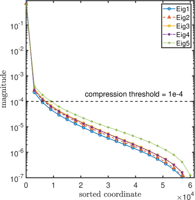
(a) h2o

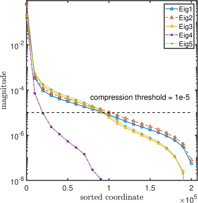
(b) ham448

Figure 1: Absolute value of each coordinate in the sorted eigenvectors. ``Eig$k$'' denotes the $k$-th smallest eigenvector.

We apply different eigensolvers to both FCI matrices, including LOBPCG in BLOPEX toolbox [24, 25], EigPen-B introduced in trace-penalty minimization [45], and our WTPM by both gradient descent (WTPM-GD) and coordinate descent (WTPM-CD) methods. The numerical results for the case $p=5$ are illustrated in Table 2. All these solvers use the same initial matrix $X^{(0)}$ which is provided by Hartree–Fock theory, and terminate when the error decreases to around $10^{-3}$. Let

(4.2) $$err^{(j)}=\max_{\ell=1,2,\dotsc,p}\absolutevalue{\lambda_{\ell}-d_{\ell}^{(j)}},$$

where $\lambda_{\ell}$, $d_{\ell}^{(j)}$ respectively denote the exact eigenvalue and the corresponding Ritz value at $j$-th iteration. As for the individual settings of each solver, in LOBPCG, the preconditioner is not used. The penalty parameter in EigPen-B is set as

(4.3) $$\mu=\max(r_{p},1).$$

The weight matrix $W$ in WTPM is set as the above statement in (4.1) and $\mu=1$.

Another thing we should emphasize is the computational complexity of each solver in one iteration. In LOBPCG, EigPen-B and WTPM-GD, the dominant cost is $2p\cdot\mathrm{nnz}(A)$ flops to obtain matrix $AX$. But WTPM-CD updates each iteration mainly at the expense of $2(p+2)\cdot\mathrm{nnz}(A_{:,\ell})$ flops, consisting of selecting largest elements index, updating $Y$ and inadequately constructing $\nabla f_{\mu,W}$. That means, on average, the complexity of updating $\tfrac{np}{p+2}$ times in WTPM-CD equals that of updating once in the other three solvers. Hence, we introduce ``relative iteration'' in WTPM-CD, which means $\tfrac{np}{p+2}$ iterations and the actual iteration number is shown in brackets in Table 2.

Table 2: A comparison of updating iterations between eigensolvers for $p=5$. The numbers in the ``WTPM-CD'' row represent relative iteration outside the bracket and actual iteration in the bracket.

		h2o		ham448
		$err$	iteration	$err$	iteration
LOBPCG		8.676e-4	18	9.929e-4	68
EigPen-B		2.971e-4	73	6.19e-4	134
WTPM-GD		4.879e-4	185	3.68e-4	191
WTPM-CD		3.901e-4	7 (283111)	7.29e-4	4 (462000)

The results in Table 2 tell us that under the requirement of $10^{-3}$ accuracy, WTPM-CD shows the efficiency applied to FCI matrices, since its theoretical complexity is much lower than the others, though the coordinate method cannot take the advantage of level-3 BLAS operations as the others and its actual runtime is longer on small systems. Instead, WTPM-GD seems not an optimal choice due to the slow convergence compared with EigPen-B and no compression of the coordinates. That is because WTPM's theoretical condition number is larger than the original trace-penalty minimization model if the elements of weight matrix $W$ differ from each other.

Furthermore, Figure 2 shows the convergence of the eigenvalues in different eigensolvers and the number of nonzero elements of the matrix $Y^{(j)}$ in WTPM-CD varying against iteration. In LOBPCG and WTPM-CD, the error monotonically decreases to the specified tolerance, but there exist spikes on the curve of error varying in EigPen-B. That is because the BB stepsize cannot guarantee monotonicity during minimization. The increasing tendency of $\mathrm{nnz}(Y^{(j)})$ in Figure 2 shows the effects of the coordinate descent method and compression update. The $\mathrm{nnz}(Y^{(j)})$ is restricted at a low level and so is the $\mathrm{nnz}(X^{(j)})$ because of the inequality $\mathrm{nnz}(Y^{(j)})\geqslant\mathrm{nnz}(X^{(j)})$ in WTPM-CD, which could significantly reduce the burden of the memory source. This is what the other eigensolvers cannot do since the matrix multiplication without compression will result in a dense matrix $AX$.

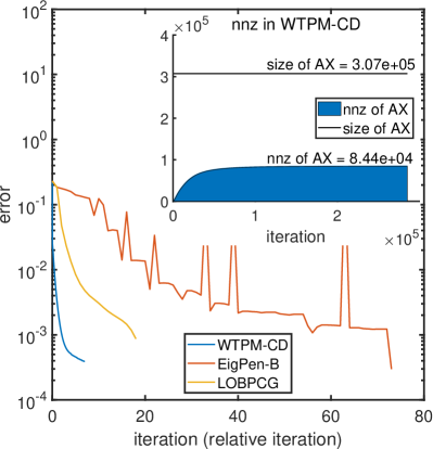
(a) h2o

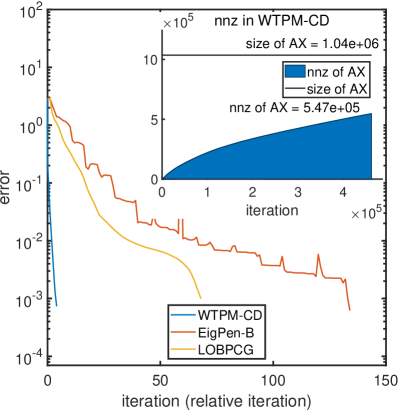
(b) ham448

Figure 2: Convergence of the smallest eigenvalues and number of nonzero elements (nnz) of the corresponding eigenvectors against iteration for $p=5$. The nnz of $AX$ in LOBPCG and EigPen-B are not shown here since it quickly increases to the maximum size of $AX$.

Besides, we apply WTPM-CD with different weight matrices $W$ to the ``h2o'' case to show the impact of $W$ on the convergence as been analyzed in Section 2.3. We use the exact eigenvalues of $A$ to generate three different weight matrices. Let $w_{1}=\tfrac{\lambda_{1}+\lambda_{n}}{2}$ and $w_{p}=\tfrac{\lambda_{p}+\lambda_{p+1}}{2}$. We set

$$\widetilde{W}: \quad w_{i}=w_{1}-(w_{1}-w_{p})\cdot\frac{i-1}{p-1},$$

$$\widehat{W}: \quad w_{i}-w_{i+1}=\left(\sum_{j=1}^{p-1}(\lambda_{j+1}-\lambda_{j})^{-1}\right)^{-1}\frac{w_{1}-w_{p}}{\lambda_{i+1}-\lambda_{i}},$$

Random : $$\quad w_{i}\text{ is uniformly distributed in the interval }(w_{p},w_{1}),$$

for $i=2,3,\dotsc,p-1$. Figure 3 shows the convergence results for different weight matrices. It follows our conclusion in Section 2.3 that $\widehat{W}$ is the best choice among the three weight matrices and $\widetilde{W}$ makes the convergence at least faster than the random choice does. In practice, if $\widehat{W}$ cannot be obtained a priori due to the cost of the construction, $\widetilde{W}$ is often found efficient enough for WTPM-CD.

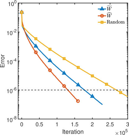
Figure 3: Convergence of the smallest eigenvalues against iteration for $p=5$ while WTPM-CD applied to ``h2o'' matrix with different weight matrices.

In summary, these examples indicate that WTPM-CD could efficiently solve the eigenvalue problem (1.1) for FCI systems, and provides an outstanding result for practical systems. In the next section, we will illustrate the performance of WTPM-CD in some larger FCI matrices of more practical interest.

4.2 Performance in Large Systems

This section provides some tests of larger FCI matrices by WTPM-CD. All programs are implemented in C++14 and compiled by Intel compiler 2021.5.0 with -O3 option. MPI and OpenMP support is disabled for all programs in this section. All of the tests in this section are produced on a machine with Intel(R) Xeon(R) Gold 6226R CPU at 2.90 GHz and 1 TB memory. The basic properties of matrices are illustrated in Table 3. Two matrices correspond to H2O and C2 molecules generated via restricted Hartree–Fock (RHF) in PSI4 package [34] with ccpVDZ atomic orbital basis set.

Table 3: Properties of Testing Molecule Systems.

Name	num of electrons	num of orbitals	matrix dimension
h2o_ccpvdz	10	24	$4.53\times 10^{8}$
c2_ccpvdz	12	28	$1.77\times 10^{10}$

In the experiments, we use the $err^{(j)}$ defined in (4.2) to measure the accuracy. Since we do not have the exact energies of excited states, we use the energies obtained by our algorithm without the compression threshold after a long enough time until the first 7 digits to the right of the decimal remain unchanged as the benchmark. The penalty parameter is simply set as $\mu=1$, and the weight matrix $W$ follows the rules in (4.1). Thus we obtain

(4.4) $$W_{h2o}=\mathrm{diag}(-75.0,-75.175,-75.35),$$

(4.5) $$W_{c2}=\mathrm{diag}(-75.138,-75.238,-75.338).$$

And in the ``h2o_ccpvdz'' case, the compression threshold is $1\times 10^{-6}$, and that in the ``c2_ccpvdz'' case is $3\times 10^{-8}$. Table 4 and Figure 4 show the convergence of WTPM-CD. The ``GS'', ``1st ES'' and ``2nd ES'' respectively denote the computed energies of the ground state, 1st excited state and 2nd excited state. The ``time'' column denotes the time of the computed energies first reaching the appointed precision, i.e., the runtime when $err^{(j)}\leqslant tol$. This practical runtime shows the efficiency of the WTPM-CD on such molecules discretized by FCI.

Table 4: Convergence of WTPM-CD.

			energy
Matrix	$p$	$tol$	GS	1st ES	2nd ES	time (s)	$\mathrm{nnz}(Y)$
h2o_ccpvdz	3	1.0e-2	-76.24141	-75.88563	-75.86844	378	5.10e07
		1.0e-3	-76.24182	-75.89341	-75.86120	2179	5.16e07
		1.0e-4	-76.24186	-75.89430	-75.86050	8653	5.16e07
c2_ccpvdz	3	1.0e-2	-75.72888	-75.63648	-75.63609	560	3.03e08
		1.0e-3	-75.73193	-75.64174	-75.63398	34248	1.26e09
		1.0e-4	-75.73196	-75.64250	-75.63327	102503	1.27e09

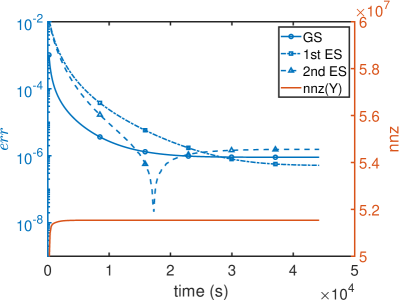
(a) h2o_ccpvdz

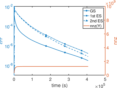
(b) c2_ccpvdz

Figure 4: Convergence of the smallest eigenvalues and number of nonzero elements (nnz) of the corresponding eigenvectors against runtime for $p=3$.

From Table 3, we can see that storing the dense matrices $X$ (or $AX$) in double type needs at least 10 GB memory for ``h2o_ccpvdz'' and 400 GB memory for ``c2_ccpvdz''. This results in the memory bottleneck of classical eigensolvers due to the unavoidable gradient calculation or orthogonalization. The nnz$(Y)$ in Table 4 tells us that under the $10^{-4}$ accuracy, the cost of memory by WTPM-CD decreases to 0.4 GB for ``h2o_ccpvdz'' and 10 GB for ``c2_ccpvdz'', which improves our capability of solving larger FCI matrices generated by more complicated particle systems. Figure 4 shows the details of the convergence, from which we can see the nnz$(Y)$ increases quickly at the beginning and is fixed at a small number in comparison with the dimension. Besides, the curve of ``2nd ES'' in Figure 4a has a different tendency from the others. That is because the energy of the 2nd excited state in ``h2o_ccpvdz'' is monotonically increasing during the iteration, and it converges to a value larger than the benchmark. It indicates that if we set a compression threshold, the converged result may lose some accuracy.

5 Conclusion

In this paper, we propose an eigensolver WTPM-CD, which is an efficient algorithm for FCI eigenvalue problems of quantum many-body systems. We first propose a novel unconstrained minimization objective, namely WTPM, for Hermitian eigenvalue problems. The theoretical analysis of the minimization model tells us that the global minimizers of WTPM are exactly the eigenvectors we expect instead of the invariant subspace, so the orthogonalization process required by other methods is not needed in WTPM. Moreover, we calculate the exact condition number of the Hessian operator, and use it to give a near-optimal weight matrix $W$. For the algorithm framework, the coordinate descent method with compression threshold reduces the number of nonzeros and the cost of storage. In numerical experiments, compared with LOBPCG and EigPen-B solvers, WTPM-CD shows a better computational complexity on small systems. On large-scale systems, WTPM-CD guarantees its efficiency while the other two solvers suffer from the bottleneck of memory.

There still exist some interesting works to be explored in the future. First, we do not give theoretical proof on the convergence of the WTPM-CD algorithm. The performance of WTPM-CD converging varies while the picking rule changes. Some in-depth research on the convergence theory is necessary to explain such a phenomenon. And some cheaper picking rules, such as stochastic search, may be introduced to the coordinate descent algorithm. The parallelization also attracts us to dive into it, since at present we can only update one element in each iteration, and the utilization efficiency of multicore is at a low level. We believe it is possible to modify the coordinate descent method to update elements in a batch and increase the parallel efficiency on shared memory systems.

References

- [1] P.-A. Absil, R. Mahony, and R. Sepulchre, Optimization Algorithms on Matrix Manifolds, Princeton University Press, Princeton, 2008, https://doi.org/10.1515/9781400830244.
- [2] A. Baiardi, C. J. Stein, V. Barone, and M. Reiher, Vibrational density matrix renormalization group, Journal of Chemical Theory and Computation, 13 (2017), pp. 3764–3777, https://doi.org/10.1021/acs.jctc.7b00329.
- [3] J. Barzilai and J. M. Borwein, Two-point step size gradient methods, IMA Journal of Numerical Analysis, 8 (1988), pp. 141–148, https://doi.org/10.1093/imanum/8.1.141.
- [4] F. A. Berezin, The Method of Second Quantization, Academic Press, New York, 1966.
- [5] N. S. Blunt, S. D. Smart, G. H. Booth, and A. Alavi, An excited-state approach within full configuration interaction quantum Monte Carlo, The Journal of Chemical Physics, 143 (2015), p. 134117, https://doi.org/10.1063/1.4932595.
- [6] G. H. Booth, A. Grüneis, G. Kresse, and A. Alavi, Towards an exact description of electronic wavefunctions in real solids, Nature, 493 (2013), pp. 365–370, https://doi.org/10.1038/nature11770.
- [7] G. H. Booth, A. J. W. Thom, and A. Alavi, Fermion Monte Carlo without fixed nodes: A game of life, death, and annihilation in Slater determinant space, The Journal of Chemical Physics, 131 (2009), p. 054106, https://doi.org/10.1063/1.3193710.
- [8] S. Boyd and L. Vandenberghe, Convex Optimization, Cambridge University Press, Cambridge, 2004.
- [9] G. K.-L. Chan and S. Sharma, The density matrix renormalization group in quantum chemistry, Annual Review of Physical Chemistry, 62 (2011), pp. 465–481, https://doi.org/10.1146/annurev-physchem-032210-103338.
- [10] Z. Chen, Y. Li, and J. Lu, On the global convergence of randomized coordinate gradient descent for non-convex optimization, 2021, https://doi.org/10.48550/ARXIV.2101.01323.
- [11] D. Cleland, G. H. Booth, and A. Alavi, Communications: Survival of the fittest: Accelerating convergence in full configuration-interaction quantum Monte Carlo, The Journal of Chemical Physics, 132 (2010), p. 041103, https://doi.org/10.1063/1.3302277.
- [12] E. U. Condon, The theory of complex spectra, Physical Review, 36 (1930), pp. 1121–1133, https://doi.org/10.1103/PhysRev.36.1121.
- [13] F. Corsetti, The orbital minimization method for electronic structure calculations with finite-range atomic basis sets, Computer Physics Communications, 185 (2014), pp. 873–883, https://doi.org/10.1016/j.cpc.2013.12.008.
- [14] B. Gao, X. Liu, X. Chen, and Y.-x. Yuan, A new first-order algorithmic framework for optimization problems with orthogonality constraints, SIAM Journal on Optimization, 28 (2018), pp. 302–332, https://doi.org/10.1137/16M1098759.
- [15] W. Gao, Y. Li, and B. Lu, Triangularized orthogonalization-free method for solving extreme eigenvalue problems, 2020, https://doi.org/10.48550/ARXIV.2005.12161.
- [16] W. Gao, Y. Li, and B. Lu, Global convergence of triangularized orthogonalization-free method, 2021, https://doi.org/10.48550/ARXIV.2110.06212.
- [17] G. H. Hardy, J. E. Littlewood, and G. Pólya, Inequalities, Cambridge Mathematical Library, Cambridge Univ. Press, Cambridge, 2nd ed., 1988.
- [18] A. A. Holmes, N. M. Tubman, and C. J. Umrigar, Heat-bath configuration interaction: An efficient selected configuration interaction algorithm inspired by heat-bath sampling, Journal of Chemical Theory and Computation, 12 (2016), pp. 3674–3680, https://doi.org/10.1021/acs.jctc.6b00407.
- [19] J. Hu, X. Liu, Z.-W. Wen, and Y.-X. Yuan, A brief introduction to manifold optimization, Journal of the Operations Research Society of China, 8 (2020), pp. 199–248, https://doi.org/10.1007/s40305-020-00295-9.
- [20] B. Huron, J. P. Malrieu, and P. Rancurel, Iterative perturbation calculations of ground and excited state energies from multiconfigurational zeroth-order wavefunctions, The Journal of Chemical Physics, 58 (1973), pp. 5745–5759, https://doi.org/10.1063/1.1679199.
- [21] P. J. Knowles and N. C. Handy, A new determinant-based full configuration interaction method, Chemical Physics Letters, 111 (1984), pp. 315–321, https://doi.org/10.1016/0009-2614(84)85513-X.
- [22] P. J. Knowles and N. C. Handy, A determinant based full configuration interaction program, Computer Physics Communications, 54 (1989), pp. 75–83, https://doi.org/10.1016/0010-4655(89)90033-7.
- [23] P. J. Knowles and N. C. Handy, Unlimited full configuration interaction calculations, The Journal of Chemical Physics, 91 (1989), pp. 2396–2398, https://doi.org/10.1063/1.456997.
- [24] A. V. Knyazev, Toward the optimal preconditioned eigensolver: Locally optimal block preconditioned conjugate gradient method, SIAM Journal on Scientific Computing, 23 (2001), pp. 517–541, https://doi.org/10.1137/S1064827500366124.
- [25] A. V. Knyazev, M. E. Argentati, I. Lashuk, and E. E. Ovtchinnikov, Block locally optimal preconditioned eigenvalue xolvers (BLOPEX) in Hypre and PETSc, SIAM Journal on Scientific Computing, 29 (2007), pp. 2224–2239, https://doi.org/10.1137/060661624.
- [26] J. D. Lee, I. Panageas, G. Piliouras, M. Simchowitz, M. I. Jordan, and B. Recht, First-order methods almost always avoid strict saddle points, Mathematical Programming, 176 (2019), pp. 311–337, https://doi.org/10.1007/s10107-019-01374-3.
- [27] Y. Li, J. Lu, and Z. Wang, Coordinatewise descent methods for leading eigenvalue problem, SIAM Journal on Scientific Computing, 41 (2019), pp. A2681–A2716, https://doi.org/10.1137/18M1202505.
- [28] L. Lin, Y. Saad, and C. Yang, Approximating spectral densities of large matrices, SIAM Review, 58 (2016), pp. 34–65, https://doi.org/10.1137/130934283.
- [29] X. Liu, Z. Wen, and Y. Zhang, An efficient Gauss–Newton algorithm for symmetric low-rank product matrix approximations, SIAM Journal on Optimization, 25 (2015), pp. 1571–1608, https://doi.org/10.1137/140971464.
- [30] J. Lu and K. Thicke, Orbital minimization method with regularization, Journal of Computational Physics, 336 (2017), pp. 87–103, https://doi.org/10.1016/j.jcp.2017.02.005.
- [31] J. Lu and Z. Wang, The full configuration interaction quantum monte carlo method through the lens of inexact power iteration, SIAM Journal on Scientific Computing, 42 (2020), pp. B1–B29, https://doi.org/10.1137/18M1166626.
- [32] K. M. Nakanishi, K. Mitarai, and K. Fujii, Subspace-search variational quantum eigensolver for excited states, Phys. Rev. Research, 1 (2019), p. 033062, https://doi.org/10.1103/PhysRevResearch.1.033062.
- [33] R. Olivares-Amaya, W. Hu, N. Nakatani, S. Sharma, J. Yang, and G. K.-L. Chan, The ab-initio density matrix renormalization group in practice, The Journal of Chemical Physics, 142 (2015), p. 034102, https://doi.org/10.1063/1.4905329.
- [34] R. M. Parrish, L. A. Burns, D. G. A. Smith, A. C. Simmonett, A. E. I. DePrince, E. G. Hohenstein, U. Bozkaya, A. Y. Sokolov, R. Di Remigio, R. M. Richard, J. F. Gonthier, A. M. James, H. R. McAlexander, A. Kumar, M. Saitow, X. Wang, B. P. Pritchard, P. Verma, H. F. I. Schaefer, K. Patkowski, R. A. King, E. F. Valeev, F. A. Evangelista, J. M. Turney, T. D. Crawford, and C. D. Sherrill, Psi4 1.1: An open-source electronic structure program emphasizing automation, advanced libraries, and interoperability, Journal of Chemical Theory and Computation, 13 (2017), pp. 3185–3197, https://doi.org/10.1021/acs.jctc.7b00174.
- [35] F. R. Petruzielo, A. A. Holmes, H. J. Changlani, M. P. Nightingale, and C. J. Umrigar, Semistochastic projector Monte Carlo method, Physical Review Letters, 109 (2012), p. 230201, https://doi.org/10.1103/PhysRevLett.109.230201.
- [36] A. Sameh and Z. Tong, The trace minimization method for the symmetric generalized eigenvalue problem, Journal of Computational and Applied Mathematics, 123 (2000), pp. 155–175, https://doi.org/10.1016/S0377-0427(00)00391-5.
- [37] J. B. Schriber and F. A. Evangelista, Adaptive configuration interaction for computing challenging electronic excited states with tunable accuracy, Journal of Chemical Theory and Computation, 13 (2017), pp. 5354–5366, https://doi.org/10.1021/acs.jctc.7b00725.
- [38] C. D. Sherrill and H. F. Schaefer, The configuration interaction method: Advances in highly correlated approaches, Advances in Quantum Chemistry, 34 (1999), pp. 143–269, https://doi.org/10.1016/S0065-3276(08)60532-8.
- [39] J. C. Slater, The theory of complex spectra, Physical Review, 34 (1929), pp. 1293–1322, https://doi.org/10.1103/PhysRev.34.1293.
- [40] J. C. Slater, A simplification of the hartree-fock method, Phys. Rev., 81 (1951), pp. 385–390, https://doi.org/10.1103/PhysRev.81.385.
- [41] N. M. Tubman, J. Lee, T. Y. Takeshita, M. Head-Gordon, and K. B. Whaley, A deterministic alternative to the full configuration interaction quantum Monte Carlo method, The Journal of Chemical Physics, 145 (2016), p. 044112, https://doi.org/10.1063/1.4955109.
- [42] E. Vecharynski, C. Yang, and J. E. Pask, A projected preconditioned conjugate gradient algorithm for computing many extreme eigenpairs of a Hermitian matrix, Journal of Computational Physics, 290 (2015), pp. 73–89, https://doi.org/10.1016/j.jcp.2015.02.030.
- [43] Z. Wang, Y. Li, and J. Lu, Coordinate descent full configuration interaction, Journal of Chemical Theory and Computation, 15 (2019), pp. 3558–3569, https://doi.org/10.1021/acs.jctc.9b00138.
- [44] Z. Wang, Z. Zhang, J. Lu, and Y. Li, Coordinate descent full configuration interaction for excited states, 2023, https://doi.org/10.48550/ARXIV.2304.13380.
- [45] Z. Wen, C. Yang, X. Liu, and Y. Zhang, Trace-penalty minimization for large-scale eigenspace computation, Journal of Scientific Computing, 66 (2016), pp. 1175–1203, https://doi.org/10.1007/s10915-015-0061-0.
- [46] S. R. White and R. L. Martin, Ab initio quantum chemistry using the density matrix renormalization group, The Journal of Chemical Physics, 110 (1999), pp. 4127–4130, https://doi.org/10.1063/1.478295.
- [47] Y. Zhou and Y. Saad, A Chebyshev–Davidson algorithm for large symmetric eigenproblems, SIAM Journal on Matrix Analysis and Applications, 29 (2007), pp. 954–971, https://doi.org/10.1137/050630404.
- [48] Y. Zhou and Y. Saad, Block Krylov–Schur method for large symmetric eigenvalue problems, Numerical Algorithms, 47 (2008), pp. 341–359, https://doi.org/10.1007/s11075-008-9192-9.