No Infinite Tail Beats Optimal Spatial Search

Abstract

Farhi and Gutmann (Physical Review A, 57(4):2403, 1998) proved that a continuous-time analogue of Grover search (also called spatial search) is optimal on the complete graphs. We extend this result by showing that spatial search remains optimal in a complete graph even in the presence of an infinitely long path (or tail). If we view the latter as an external quantum system that has a limited but nontrivial interaction with our finite quantum system, this suggests that spatial search is robust against a coherent infinite one-dimensional probe. Moreover, we show that the search algorithm is oblivious in that it does not need to know whether the tail is present or not, and if so, where it is attached to.

I Introduction

The celebrated quantum search algorithm of Grover [12] provides a provable quadratic speedup over any classical algorithm. Shortly thereafter, Farhi and Gutmann proposed an analogue analog of Grover’s algorithm [8]. They defined the Grover search algorithm via a continuous-time quantum walk on a complete graph where the oracle or target vertex is marked by a suitably weighted self-loop. Remarkably, the Farhi-Gutmann algorithm achieved perfect fidelity on complete graphs of any size. In contrast, this property does not hold for Grover search (viewed as a discrete-time quantum walk) as it is inherently a bounded-error probabilistic algorithm.

This continuous-time search problem was later generalized by Childs and Goldstone [6] to arbitrary finite graphs where it is known as the spatial search problem. A collection of different families of finite graphs had been studied in this context; for example, see [6, 13, 21, 9, 4, 19]. But, to date, spatial search has not been studied on infinite graphs as it seems that the quantum walk will escape or diffuse to infinity before having a chance to localize on the marked vertex (or oracle). The goal of this work is to disabuse ourselves of this highly plausible intuition.

We consider infinite graphs which are obtained by attaching an infinite path (or tail) to a finite graph. This family of graphs with tails was explored by Golinskii [11]. In this work, we view the finite graph as our operational quantum system for performing quantum search and the tail as an external (possibly, adversarial) infinite-dimensional quantum system which interacts with our finite sytem in a coherent manner.

The main question we explore in this work is: can spatial search still be performed optimally in the presence of an infinite-dimensional probe? We provide a positive answer to this question for complete graphs. This extends the result of Farhi-Gutmann [8] to the infinite setting. Moreover, the quantum search algorithm is oblivious as it does not need to know whether the infinite-dimensional probe is present (or not) and where it is attached to (if present). Since we give our adversary the benefit of an infinite-dimensional quantum system, this serves only to strengthen the result.

Our technique relies on the theory of Jacobi operators (see [11, 7]). The main idea is to decompose the adjacency operator $A$ of our infinite graph using two pairwise orthogonal invariant subspaces (see Golinskii [11], Theorem 1.2) where the first one is finite-dimensional while the second one is infinite-dimensional. The next crucial observation is that spatial search takes place in the infinite-dimensional invariant subspace of $A$. Moreover, the action of $A$ in this infinite-dimensional invariant subspace is given by a finite rank Jacobi matrix $J$. Finally, we show that the initial and target states of the spatial search are nearly confined in a two-dimensional subspace spanned by two bound states of $J$. This yields the claimed spatial search result. To the best of our knowledge, this is the first result which explores optimal spatial search on infinite graphs.

As outlined above, our argument is the standard argument for showing optimal spatial search in the finite setting (see [3, 4, 5]). Namely, we show that the initial and target states are spanned by two distinct eigenvectors of the perturbed adjacency matrix. A contribution of this work is to show that this argument holds in the infinite setting via bound states of the reduced adjacency operator. We believe that this argument might be useful in other settings.

Following a brief discussion of basic notation and terminology in Section II, we prove our main results in Sections III and IV. Then, we justify the optimality of our search algorithm in Section V. Finally, we conclude with some open questions in Section VI.

II Preliminaries

We introduce the basic notation and terminology that we will use throughout. The set of all positive integers is denoted $\mathbb{Z}^{+}$ and the set of all complex numbers with unit modulus is denoted $U(1)$. For vectors $x,y$ where $x=\zeta y$, for some $\zeta\in U(1)$, we write $x\equiv y$. We adopt standard asymptotic notation: $o(f_{n})$ denotes any function $g_{n}$ so that $g_{n}/f_{n}\to 0$, $\mathcal{O}(f_{n})$ denotes functions $g_{n}$ for which $g_{n}/f_{n}$ is bounded from above by a constant, and $\Omega(f_{n})$ denotes functions $g_{n}$ where $g_{n}/f_{n}$ is bounded from below by a constant, where in each case $n\to\infty$; see [20]. In our case, the asymptotic parameter $n$ corresponds to the size of a finite graph.

Graphs and operators.

We study undirected and connected graphs $G=(V,E)$ with vertex set $V$ and edge set $E$, respectively. The adjacency matrix $A$ of $G$ is a symmetric matrix whose $(i,j)$ entry is $1$ if $(i,j)\in E$ and $0$ otherwise. For a vertex $u$, let $N(u)=\{v\in V:(u,v)\in E\}$ denote the set of neighbors of $u$. The degree of vertex $u$, denoted $\deg(u)$, is the cardinality of $N(u)$. The complete graph (or clique) on $n$ vertices is denoted $K_{n}$. A rooted graph $(G,r)$ is a graph $G$ with a distinguished vertex $r$ which we call the root. See [10] for further background on algebraic graph theory.

We allow countably infinite graphs, in which case, $V=\mathbb{Z}^{+}$ (see [16]). For example, the infinite path $P_{\infty}$ has edges which are consecutive positive integers; its adjacency matrix is known as the free Jacobi matrix (see [11]). Related to these graphs, we associate a complex separable Hilbert space $\mathcal{H}=\ell^{2}(V)$ equipped with the inner product $\langle x,y\rangle=\sum_{u\in V}\overline{x_{u}}y_{u}$, for vectors $x,y\in\mathcal{H}$. For $\ell^{2}(V)$, a standard basis is $\{e_{u}:u\in V\}$, where $e_{u}$ is the unit vector corresponding to vertex $u$. An infinite graph $\mathcal{G}$ is locally finite if $\deg{(u)}<\infty$ for all $u\in V$. For such a graph $\mathcal{G}$, the adjacency operator $A$ is a linear operator that maps the standard basis vector $e_{v}$ to the vector associated with the neighboring vertices $N(v)$; that is, $Ae_{v}=\sum_{u\in N(v)}a_{u,v}e_{u}$, or simply $a_{u,v}=\langle e_{u},Ae_{v}\rangle$. Let $\deg{(\mathcal{G})}=\sup\{\deg{(u)}:u\in V\}$. If $\deg(\mathcal{G})<\infty$, then the adjacency operator $A$ is a bounded self-adjoint operator (see [15]).

The spectrum of a linear operator $A$ is the set $\sigma(A)$ of all complex numbers $\lambda$ where $\lambda I-A$ is not invertible. For a bounded and self-adjoint operator $A$, its spectrum can be classified further into the point spectrum $\sigma_{p}(A)$ and the continuous spectrum $\sigma_{c}(A)$. The point spectrum consists of all eigenvalues $\lambda\in\mathbb{C}$ of $A$ such that $Ax=\lambda x$ for some nonzero $x\in\ell^{2}(V)$. On the contrary, the values in $\sigma_{c}(A)$ are not eigenvalues of $A$ and have no corresponding eigenvectors in $\ell^{2}(V)$.

The spectral theorem (see [1, 17]) states that for a bounded self-adjoint operator $A$ on a complex Hilbert space $\mathcal{H}$, there exists a unique resolution of the identity $E$ on the Borel subsets of $\sigma(A)$ so that $A=\int_{\sigma(A)}\lambda\ dE(\lambda)$. Moreover, if $f$ is a bounded Borel function on $\sigma(A)$, then $f(A)=\int_{\sigma(A)}f(\lambda)\ dE(\lambda)$. We also use a decomposition induced by invariant subspaces (see [1], Theorem 3, section 40) which states that if $W_{k}$ $(k=1,2,\cdots,m)$ are pairwise orthogonal invariant subspaces of $A$, that is, $\mathcal{H}=\bigoplus_{k=1}^{m}W_{k}$ and $AW_{k}\subset W_{k}$, for each $k$, then $A=\sum_{k=1}^{m}A_{k}P_{k}$, where $P_{k}$ is the projection on $W_{k}$ and $A_{k}$ is the restriction of $A$ to $W_{k}$.

Spatial Search.

A continuous-time quantum walk on an infinite graph $\mathcal{G}$ with bounded self-adjoint adjacency operator $A$ is given by the unitary operator $e^{-itA}$ (acting on the Hilbert space $\ell^{2}(V)$). Our focus is on infinite graphs obtained from a finite connected rooted graph $(G,r)$ by attaching an infinite path $P_{\infty}$ at the root vertex $r$; denote the resulting infinite graph as $\mathcal{G}=G(r,P_{\infty})$. As we use $\{1,2,\ldots,n\}$ to label the vertices of a finite rooted graph of order $n$, we take the liberty to designate the last vertex $n$ as the root (without loss of generality). These are the graphs with tails studied by Golinskii [11].

We say the infinite graph $\mathcal{G}=G_{n}(P_{\infty})$ has optimal spatial search (adopting [4]) if there is a real $\gamma>0$ so that for each vertex $w$ of $G_{n}$, a continuous-time quantum walk on $\mathcal{G}$ with a self-loop on $w$ of weight $\gamma$ will unitarily map the principal eigenvector $z_{1}$ of $G_{n}$ to the unit vector $e_{w}$ with constant fidelity in time $t=\mathcal{O}(1/\epsilon_{1})$, where $\epsilon_{1}=|\langle e_{w},z_{1}\rangle|$. That is,

$$\left|\langle e_{w},e^{-it(A+\gamma P_{w})}z_{1}\rangle\right|=\Omega(1),$$

where $A$ is the adjacency operator of $\mathcal{G}$ and $P_{w}$ is the projection onto the subspace spanned by $e_{w}$. It is customary to assume $\epsilon_{1}=o(1)$ as otherwise we already have a constant overlap between the target state $e_{w}$ and the initial state $z_{1}$.

III Infinite lollipop is optimal

For $n\geq 2$, consider the infinite lollipop graph $\mathcal{L}_{n}=K_{n}(P_{\infty})$. The vertices of the infinite path $P_{\infty}$ are labelled with $n+1,n+2,\ldots$. To this lollipop graph $\mathcal{L}_{n}$, we place a self-loop of weight $\gamma$ at vertex $1$ (the oracle or target vertex) and denote the resulting infinite graph as $\mathcal{L}_{n}(\gamma)$. Please see Figure 1.

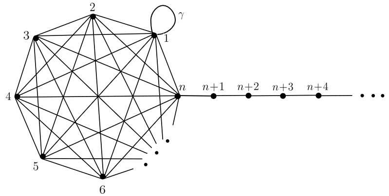
Figure 1: Optimal spatial search on the infinite lollipop with the oracle hiding at vertex $1$.

The adjacency operator $H$ of $\mathcal{L}_{n}(\gamma)$ is obviously a bounded self-adjoint linear operator on $l^{2}(\mathbb{Z}^{+})$. It can be written as an infinite dimensional matrix under the standard basis $\{e_{j}\}_{j=1}^{\infty}$ as

$$H=\begin{pmatrix}\gamma&1&\cdots&1&&&&\\ 1&0&\cdots&1&&&&\\ \vdots&\vdots&\ddots&\vdots&&&&\\ 1&1&\cdots&0&1&&&&\\ &&&1&\ 0&1&&\\ &&&&\ 1&0&1&\\ &&&&&\ddots&\ddots&\ddots\end{pmatrix}.$$

Our goal is to prove the following infinite analogue of the Farhi-Gutmann result.

Theorem 1.

For $\gamma=n+\mathcal{O}(1)$, we have

$$|\langle e_{1},e^{-itH}z_{1}\rangle|=\Omega(1),$$

for $t=\pi/2\sqrt{n}$, where $z_{1}=n^{-1/2}\sum_{j=1}^{n}e_{j}$.

By a theorem of Golinskii ([11], Theorem 1.2), using a change of basis, $H$ can be written in a block diagonal form. This new basis $\{\tilde{e}_{k}\}_{k=1}^{\infty}$ is defined as follows. Let

$$\tilde{e}_{k}=e_{k},\ \ k=n,n+1,\cdots$$ (1)

and

$$\tilde{e}_{n-1}=\frac{1}{\sqrt{n-1}}\sum_{j=1}^{n-1}e_{j}.$$ (2)

The next orthogonal basis vector is then given by

$$\tilde{e}_{n-2}^{\prime} =H\tilde{e}_{n-1}-\langle\tilde{e}_{n-1},H\tilde{e}_{n-1}\rangle\tilde{e}_{n-1}-\langle\tilde{e}_{n},H\tilde{e}_{n-1}\rangle\tilde{e}_{n}.$$

which, after normalization, yields

$$\tilde{e}_{n-2}=\frac{1}{\sqrt{(n-2)(n-1)}}((n-1)e_{1}-\tilde{e}_{n-1}).$$ (3)

We take the remaining basis vectors to be the non-principal columns of the Fourier matrix of order $n-2$. In particular, the basis vector $\tilde{e}_{k}$ is defined as

$$\tilde{e}_{k}=\frac{1}{\sqrt{n-2}}\sum_{j=1}^{n-2}e^{\frac{2\pi i(j-1)k}{(n-2)}}e_{j}\ \ \ (k=1,\ldots,n-3).$$

Since $H\tilde{e}_{n-2}=\left(\gamma\frac{n-2}{n-1}-1\right)\tilde{e}_{n-2}+\gamma\frac{\sqrt{n-2}}{n-1}\tilde{e}_{n-1}$, the subspace $\mathcal{S}=\operatorname{span}\{\tilde{e}_{n-2},\tilde{e}_{n-1},\cdots\}$ is $H$-invariant. Under the new basis, the adjacency operator $H$ becomes

$$H=\begin{pmatrix}-I_{n-2}&O\\ O&\widehat{H}\end{pmatrix}$$

As will be clear soon, it suffices for us to restrict our focus on the operator $\widehat{H}$, which is the operator $H$ restricted to the subspace $\mathcal{S}=\operatorname{span}\{\tilde{e}_{n-2},\tilde{e}_{n-1},\cdots\}$. This is because the initial state $z_{1}$ and the target state $e_{1}$ of our spatial search problem both have non-negligible overlap with $\mathcal{S}$.

It follows from the preceding analysis that the operator $H$ under the basis $\{\tilde{e}_{n-2},\tilde{e}_{n-1},\ldots\}$ is given by

$$\widehat{H}=\begin{array}[]{rl}\begin{matrix}{\scriptstyle\tilde{e}_{n-2}}\\ {\scriptstyle\tilde{e}_{n-1}}\\ {\scriptstyle\tilde{e}_{n}}\\ {\scriptstyle\tilde{e}_{n+1}}\\ \vdots\end{matrix}\!\!\!\!\!&\begin{pmatrix}\gamma\frac{n-2}{n-1}\!-\!1&\gamma\frac{\sqrt{n-2}}{n-1}&&&&&\\ \gamma\frac{\sqrt{n-2}}{n-1}&n\!\!-\!\!2\!+\!\frac{\gamma}{n-1}&\sqrt{n\!\!-\!\!1}&&&&\\ &\sqrt{n\!\!-\!\!1}&0&1&&&\\ &&1&0&\ \ 1&&\\ &&&\ddots&\ddots&\ddots\end{pmatrix}.\end{array}$$ (5)

This symmetric tridiagonal matrix is an eventually-free or finite rank Jacobi matrix (see [11]) whose full spectrum can be computed via the so-called Jost solution (see [7], Appendix). The Jost solution is a vector $y(x)=(y_{1}(x),y_{2}(x),\cdots)^{T}$ that satisfies the eigen-equation of $\widehat{H}$ with eigenvalue of the form $x+\frac{1}{x}$, namely,

$$\widehat{H}y(x)=\left(x+\frac{1}{x}\right)y(x),$$ (6)

and also the degree condition

$$\lim_{k\to\infty}x^{-k}y_{k}(x)=1.$$

Given the special form of $\widehat{H}$, we can set

$$y_{k}(x)=x^{k},\ \ k=3,4,\cdots,$$ (7)

and use (6), to get the Jost polynomial

$$y_{0}(x) =\frac{1}{\gamma}\sqrt{\frac{n-1}{n-2}}\cdot\left[(2-n)x^{4}+[(n-3)\gamma+4-2n)]x^{3}\right.$$

$$+\left.[(n-3)\gamma+5-2n]x^{2}+[3-n-\gamma]\,x+1\right].$$ (8)

In order to compute the eigenvalues of $\widehat{H}$, we need the following spectral theorem for finite rank Jacobi operators. We will only need information about the point spectrum as will be clear soon.

Theorem 2.

([11], p8) Let $J$ be an eventually-free Jacobi matrix and $y_{0}(x)$ be its Jost function. Then all roots of $y_{0}(x)$ in the complex unit disk are real and simple, $y_{0}(0)\not=0$. A real number $\lambda_{j}$ is an eigenvalue of $J$ if and only if

$$\lambda_{j}=x_{j}+\frac{1}{x_{j}},\quad x_{j}\in(-1,1),\quad y_{0}(x_{j})=0.$$

By choosing $\gamma=n+\mathcal{O}(1)$, the roots of $y_{0}(x)$ in the complex unit disk can be approximated consecutively. First note that there are four real roots for $y_{0}(x)$ and two of them lie in the unit disk as indicated by the following table:

$x$	$-\infty$	$-1$	${\scriptstyle\frac{1}{n}}$	$1$	$+\infty$
${\gamma}{\scriptstyle\sqrt{\frac{n-2}{n-1}}}\cdot y_{0}$	$-\infty$	$\gamma\!+\!1\!>\!0$	${\scriptstyle-\frac{1}{n}+\mathcal{O}(\frac{1}{n^{\scriptscriptstyle 2}})}\!<\!0$	$2n\gamma\!+\!{\scriptstyle\mathcal{O}(n)}\!>\!0$	$-\infty$

Table 1: For $\gamma=n+\mathcal{O}(1)$ and sufficiently large $n$, there are $4$ sign changes of $y_{0}(x)$.

Denote the two roots within the unit disk as $x_{\pm}=\frac{1}{n}+\delta_{\pm}$. Hence,

$$0 ={\gamma}\sqrt{\frac{n-2}{n-1}}\cdot y_{0}(x_{\pm})=-\frac{1}{n}+n^{2}\delta_{\pm}^{2}+o\left(\frac{1}{n}\right)+o(n^{2}\delta_{\pm}^{2}).$$

In order for the left-hand side to attain $0$ exactly, for all $n$, at least the two highest order terms on the right-hand side should cancel perfectly; that is, $o(\frac{1}{n})=-\frac{1}{n}+n^{2}\delta_{\pm}^{2}$ which implies

$$x_{\pm}=\frac{1}{n}\pm\frac{1}{n^{3/2}}+o\left(\frac{1}{n^{3/2}}\right).$$ (9)

Therefore, the two distinct eigenvalues of $\widehat{H}$ are given by

$$\lambda_{\pm}=n\pm\sqrt{n}+\mathcal{O}(1).$$ (10)

The corresponding eigenvectors (or bound states) are given by $y_{\pm}=(y_{1}(x_{\mp}),y_{2}(x_{\mp}),\ldots)^{T}$ where the entries are defined by the Jost polynomials

$$y_{1}(x_{\mp}) =\pm\frac{1}{\gamma}\sqrt{\frac{n-1}{n-2}}\cdot\frac{1}{n^{3/2}}+\mathcal{O}\left(\frac{1}{n^{3}}\right),$$ (11)

$$y_{2}(x_{\mp}) =\frac{1}{\sqrt{n-1}}\cdot\frac{1}{n^{2}}\mp\frac{1}{\sqrt{n-1}}\frac{2}{n^{5/2}}+\mathcal{O}\left(\frac{1}{n^{7/2}}\right),$$ (12)

$$y_{k}(x_{\mp}) =\frac{1}{n^{k}}\mp\frac{k}{n^{(2k+1)/2}}+\mathcal{O}\left(\frac{1}{n^{k+1}}\right),\quad k=3,4,\cdots.$$ (13)

Now, we are ready to prove Theorem 1.

First, note that both $e_{1}=\sqrt{\frac{1}{n-1}}\tilde{e}_{n-2}+\sqrt{\frac{n-2}{n-1}}\tilde{e}_{n-1}$ and $z_{1}=\tilde{e}_{n-1}$ are completely in the invariant subspace $\mathcal{S}$. Thus, we can restrict our unitary evolution to $\mathcal{S}$. Moreover, as $e_{1}$ overlaps almost completely with $\tilde{e}_{n-1}$, it suffices to consider $\tilde{e}_{n-1}$ as the target state. Hence, the fidelity can be further approximated as

$$\left|\langle e_{1},e^{-itH}z_{1}\rangle\right|\geq\sqrt{\frac{n-2}{n-1}}\left|\langle\overline{e}_{1},e^{-it\widehat{H}}\overline{e}_{2}\rangle\right|+\mathcal{O}\left(\frac{1}{n^{1/2}}\right),$$

where $\overline{e}_{k}$ is a unit vector which is the $k$-th basis vector for the invariant subspace $\mathcal{S}=\operatorname{span}\{\tilde{e}_{n-2},\tilde{e}_{n-1},\cdots\}$.

Notice that

$$\mathop{\mathrm{\lim}}\limits_{n\rightarrow\infty}{\frac{\langle\overline{e}_{k},y_{+}\rangle\langle y_{+},\overline{e}_{k}\rangle}{\langle y_{+},y_{+}\rangle}+\frac{\langle\overline{e}_{k},y_{-}\rangle\langle y_{-},\overline{e}_{k}\rangle}{\langle y_{-},y_{-}\rangle}}=1,\ \ k=1,2,$$

that is, both the initial and the target states lie in the two-dimensional invariant subspace spanned by the eigenvectors $y_{+}$ and $y_{-}$. Thus, it again suffices to consider the fidelity in this subspace.

Straightforward calculation shows that when $\gamma=n+\mathcal{O}(1)$, the fidelity satisfies $|\langle e_{1},e^{-itH}z_{1}\rangle|=1+o(1)$ for time $t=\frac{\pi}{2\sqrt{n}}$. If we normalize the adjacency matrix of $K_{n}$, we obtain $\mathcal{O}(\sqrt{n})$ time (matching Grover search).

IV Oracle at the edge of infinity

In this section, we show that even when the oracle is placed at the attachment vertex of the infinite path, spatial search remains optimal on $\mathcal{L}_{n}$. See Figure 2.

Together with Section III, this will show that the search algorithm is oblivious as it does not need to know if the external probe (tail) is present or not. This is because the two cases surprisingly require the same asymptotic time for optimal spatial search. The claim follows from a similar analysis as before.

The adjacency operator of $\mathcal{L}_{n}(\gamma)$ is given as

$$H=\begin{pmatrix}0&1&\cdots&1&&&&\\ 1&0&\cdots&1&&&&\\ \vdots&\vdots&\ddots&\vdots&&&&\\ 1&1&\cdots&\gamma&1&&&&\\ &&&1&\ 0&1&&\\ &&&&\ 1&0&1&\\ &&&&&\ddots&\ddots&\ddots\end{pmatrix}.$$

First, we restrict our focus to the invariant subspace $\mathcal{S}=\operatorname{span}\{\tilde{e}_{n-1},\tilde{e}_{n},\cdots\}$ since $e_{n}=\tilde{e}_{n}\in\mathcal{S}$ and $z_{1}=\sqrt{\frac{n-1}{n}}\tilde{e}_{n-1}+\sqrt{\frac{1}{n}}\tilde{e}_{n}\in\mathcal{S}$, where $\tilde{e}_{n-1}=\frac{1}{\sqrt{n-1}}\sum_{j=1}^{n-1}e_{j}$ and $\tilde{e}_{k}=e_{k}$, $k\geq n$. Under the new basis that spans $\mathcal{S}$, the operator $H$ is a rank-$2$ Jacobi matrix

$$\widehat{H}=\begin{array}[]{rl}\begin{matrix}{\scriptstyle\tilde{e}_{n-1}}\\ {\scriptstyle\tilde{e}_{n}}\\ {\scriptstyle\tilde{e}_{n+1}}\\ \vdots\end{matrix}\!\!\!\!\!&\begin{pmatrix}n\!\!-\!\!2\!&\sqrt{n\!\!-\!\!1}&&&&\\ \sqrt{n\!\!-\!\!1}&\gamma&1&&&\\ &1&0&\ \ 1&&\\ &&\ddots&\ddots&\ddots\end{pmatrix}.\end{array}$$ (15)

Hence, the following Jost polynomials are obtained:

$$y_{0}(x) =\frac{1}{\sqrt{n-1}}\cdot[-\gamma x^{3}+(n-2)(\gamma-1)x^{2}$$

$$\ \ \ \ \ \ \ \ \ \ \ \ \ \ \ \ \ +(2-n-\gamma)x+1],$$ (16)

$$y_{1}(x) =\frac{1}{\sqrt{n-1}}\cdot(x-\gamma x^{2}),$$ (17)

$$y_{k}(x) =x^{k},\ \ k=2,3,\cdots.$$ (18)

By choosing $\gamma=n+\mathcal{O}(1)$, we can compute the two distinct roots for $y_{0}$ that is within the interval $[-1,1]$

$$x_{\pm}=\frac{1}{n}\pm\frac{1}{n^{3/2}}+o\left(\frac{1}{n^{3/2}}\right),$$ (19)

which yields the corresponding eigenvalues for $\widehat{H}$

$$\lambda_{\pm}=n\pm\sqrt{n}+\mathcal{O}(1).$$ (20)

As shown previously, the corresponding eigenvectors are defined by the values of Jost polynomials:

$$y_{1}(x_{\mp}) =\pm\frac{1}{\sqrt{n-1}}\cdot\frac{1}{n^{3/2}}+\mathcal{O}\left(\frac{1}{n^{5/2}}\right)$$ (21)

$$y_{2}(x_{\mp}) =\frac{1}{n^{2}}\mp\frac{2}{n^{5/2}}+\mathcal{O}\left(\frac{1}{n^{3}}\right)$$ (22)

$$y_{k}(x_{\mp}) =\frac{1}{n^{k}}\mp\frac{k}{n^{(2k+1)/2}}+\mathcal{O}\left(\frac{1}{n^{k+1}}\right),\ \ k=3,4,\cdots.$$ (23)

Following the same argument, we can see that for time $t=\frac{\pi}{2\sqrt{n}}$, the fidelity satisfies $|\langle e_{n},e^{-itH}z_{1}\rangle|=1+o(1)$.

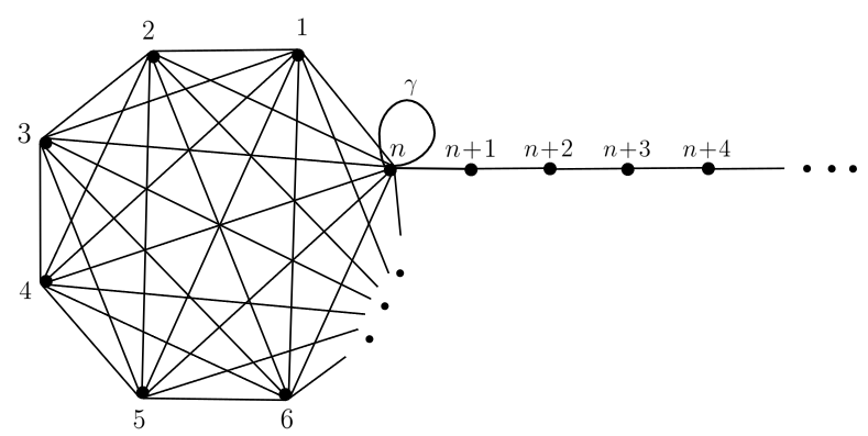
Figure 2: Optimal spatial search still occurs on the infinite lollipop even if the oracle sits at gateway vertex $n$.

V Optimality

We show that the time bound obtained in Theorem 1 (and in Section IV) is optimal. To this end, we generalize an argument of Farhi and Gutmann [8] to a class of infinite graphs with tails.

For a finite graph $G_{n}$ on $n$ vertices, take the cone $\widehat{G}_{n}=K_{1}+G_{n}$ which is obtained by adding a new vertex (called the conical vertex) and connecting it to all vertices of $G_{n}$. Then, attach a tail to the conical vertex and denote this infinite graph as $\widehat{G}_{n}(P_{\infty})$. Notice that we recover the infinite lollipop when $G_{n}$ is a clique.

Theorem 3.

Let $G_{n}$ be a $(n,d)$-regular graph, where $d=\omega(\sqrt{n})$ for some $\delta>0$, and let $\mathcal{H}_{0}$ be the adjacency operator of $\widehat{G}_{n}(P_{\infty})$. Let $z_{1}\in\ell^{2}$ being natural embedding of the principal eigenvector of $G_{n}$. Suppose there is a time $t_{0}$ so that for some $\gamma\in\mathbb{R}$ and $\zeta\in U(1)$, and for a vertex $w$ of $G_{n}$, we have

$$\left\lVert e^{-it_{0}(\mathcal{H}_{0}+\gamma P_{w})}z_{1}-\zeta e_{w}\right\rVert^{2}=o(1).$$

Then, $\gamma t_{0}=\Omega(1/\epsilon_{1})$, where $\epsilon_{1}=|\langle e_{w},z_{1}\rangle|$, provided $1/\gamma\epsilon_{1}\in o(1)$.

The largest eigenvalue in $\sigma_{p}(\mathcal{H}_{0})$ has a unique bound eigenstate $\beta_{1}$ which satisfies $\left\lVert\beta_{1}-z_{1}\right\rVert=o(1)$. This can be shown using similar techniques as in previous sections.

We call a time-dependent state $\psi(t)\in\ell^{2}(\mathbb{Z}^{+})$ exponentially decaying if there is a positive integer $M$ so that for all $m\geq M$ we have $|\langle e_{m},\psi(t)\rangle|=\mathcal{O}(\kappa^{m})$, for some $\kappa<1$, for all $t$.

Proof.

(of Theorem 3) Let $\mathcal{H}_{w}=\mathcal{H}_{0}+\gamma P_{w}$. It suffices to show the claim under the assumption $\left\lVert e^{-it\mathcal{H}_{w}}\beta_{1}-\zeta e_{w}\right\rVert^{2}=o(1)$, since $\left\lVert\beta_{1}-z_{1}\right\rVert=o(1)$ and by using the triangle inequality for squared norm (see [18], eq. 18.5).

Following [8], we compare two Schrödinger evolutions given by

$$\psi_{w}^{\prime}(t) =-i\mathcal{H}_{w}\psi_{w}(t), \psi_{w}(0)=\beta_{1},$$

$$\psi_{0}^{\prime}(t) =-i\mathcal{H}_{0}\psi_{0}(t), \psi_{0}(0)=\beta_{1}.$$

Note $\psi_{0}(t)\equiv\beta_{1}$, for all $t$, as $\beta_{1}$ is an eigenstate of $\mathcal{H}_{0}$.

For simplicity, we assume that spatial search achieves perfect fidelity, namely, $\psi_{w}(t_{0})\equiv e_{w}$. The general case is handled using triangle inequality for squared norm.

The key quantity is $M(t):=\left\lVert\psi_{w}(t)-\psi_{0}(t)\right\rVert^{2}$. First, notice that

$$M(t_{0}) =2(1-\mathtt{Re}\langle e_{w},\beta_{1}\rangle)\geq 2(1-\epsilon_{1}).$$ (24)

Furthermore, we have $M^{\prime}(t)=-2\mathtt{Re}\langle\psi_{w}(t),\psi_{0}(t)\rangle^{\prime}$. Given that the inner product is an infinite series, the existence of its derivative requires uniform convergence. As $\psi_{0}(t)\equiv\beta_{1}$ is exponentially decaying (by virtue of being a Jost solution), we have $|\overline{(\psi_{w}(t))_{m}}(\beta_{1})_{m}|\leq|(\beta_{1})_{m}|$ and

$$\sum_{m=1}^{\infty}|(\beta_{1})_{m}|\leq C_{M}+\sum_{m\geq M}\kappa^{m}=C_{M}+\frac{\kappa^{M}}{1-\kappa}<\infty$$

for a constant $C_{M}$. Thus, $\langle\psi_{w}(t),\beta_{1}\rangle$ is uniformly convergent (see Titchmarsh [20], 1.11).

Since $\mathcal{H}_{w}$ is a finite-rank Jacobi matrix and $\psi^{\prime}_{w}(t)=-i\mathcal{H}_{w}\psi_{w}(t)$, we see that $\langle\psi^{\prime}_{w}(t),\psi_{0}(t)\rangle$ is also uniformly convergent. This allows us to take the derivative of $\langle\psi_{w}(t),\psi_{0}(t)\rangle$ by termwise differentiation (see Titchmarsh [20], 1.72), i.e.,

$$\langle\psi_{w}(t),\psi_{0}(t)\rangle^{\prime} \!=\!\langle\psi_{w}(t),\psi^{\prime}_{0}(t)\rangle\!+\!\langle\psi^{\prime}_{w}(t),\psi_{0}(t)\rangle$$

$$\!=\!-i\langle\psi_{w}(t),\mathcal{H}_{0}\psi_{0}(t)\rangle\!+\!i\langle\mathcal{H}_{w}\psi_{w}(t),\psi_{0}(t)\rangle.$$

So, we obtain

$$M^{\prime}(t)=2\gamma\mathtt{Im}\langle P_{w}\psi_{w}(t),\psi_{0}(t)\rangle\leq 2\gamma\left\lVert P_{w}\psi_{0}(t)\right\rVert.$$

Thus, $M^{\prime}(t)\leq 2\gamma\epsilon_{1}$, which further implies

$$M(t_{0})=\int_{0}^{t_{0}}M^{\prime}(t)dt\leq 2\gamma\epsilon_{1}t_{0}.$$

By combining the lower and upper bounds on $M(t_{0})$, we get $\gamma t_{0}\geq(1-\epsilon_{1})/\epsilon_{1}=\Omega(1/\epsilon_{1})$ as $\epsilon_{1}=o(1)$. ∎

Theorem 3 justifies the optimal time $1/\epsilon_{1}$ used to define spatial search. For the infinite lollipop, we have $\epsilon_{1}=1/\sqrt{n}$, and thus, $\gamma t_{0}=\Omega(\sqrt{n})$. Since the search algorithm uses $\gamma=n+\mathcal{O}(1)$, we get $t_{0}=\Omega(1/\sqrt{n})$, which matches the bound achieved by Theorem 1. Hence, the algorithm is optimal.

VI Conclusion

In this work, we proved optimal spatial search occurs on cliques even in the presence of an infinite path. This generalized a known result of Farhi and Gutmann [8] to the infinite setting. We view this as a first step in showing that optimal spatial search is robust against an adversary modeled as an infinite-dimensional external quantum probe. Interesting directions for future work include extending the result to multiple tails or to tails induced by more general Jacobi matrices and strengthening the lower bound to other families of infinite graphs.

Our work was motivated by a question posed in [2]. We mention that discrete-time quantum walk on graphs with tails was studied in [14].

References

• [1] N.I. Akhiezer and I.M. Glazman. Theory of linear operators in Hilbert space. Courier Corporation, 2013.
• [2] P.-A. Bernard, C. Tamon, L. Vinet, and W. Xie. Quantum state transfer in graphs with tails, 2022. arxiv:quant-ph/2211.14704.
• [3] S. Chakraborty, L. Novo, A. Ambainis, and Y. Omar. Spatial search by quantum walk is optimal for almost all graphs. Physical Review Letters, 116(3):100501, 2016.
• [4] S. Chakraborty, L. Novo, and J. Roland. Optimality of spatial search via continuous-time quantum walks. Physical Review A, 102(3):032214, 2020.
• [5] A. Chan, C. Godsil, C. Tamon, and W. Xie. Of shadows and gaps in spatial search. Quantum Information and Computation, 22(13& 14):1110–1131, 2022.
• [6] A. Childs and J. Goldstone. Spatial search by quantum walk. Physical Review A, 70:022314, 2004.
• [7] D. Damanik and B. Simon. Jost functions and Jost solutions for Jacobi matrices, II. Decay and Analyticity. International Mathematics Research Notices, 2006:19396, 2006.
• [8] E. Farhi and S. Gutmann. Analog analogue of a digital quantum computation. Physical Review A, 57(4):2403, 1998.
• [9] A. Glos and T. Wong. Optimal quantum walk search on Kronecker graphs with dominant or fixed regular initiators. Physical Review A, 98:062334, 2018.
• [10] C. Godsil and G. Royle. Algebraic Graph Theory. Springer, 2001.
• [11] L. Golinskii. Spectra of infinite graphs with tails. Linear and Multilinear Algebra, 64(11):2270–2296, 2016.
• [12] L. Grover. Quantum mechanics help in searching for a needle in a haystack. Physical Review Letters, 79:325, 1997.
• [13] J. Janmark, D. Meyer, and T. Wong. Global symmetry is not necessary for fast quantum search. Physical Review Letters, 112:210502, 2014.
• [14] N. Konno, E. Segawa, and M. Štefaňák. Relation between quantum walks with tails and quantum walks with sinks on finite graphs, 2021. arxiv:math-ph/2105.03111.
• [15] B. Mohar. The spectrum of an infinite graph. Linear algebra and its applications, 48:245–256, 1982.
• [16] B. Mohar and W. Woess. A survey on spectra of infinite graphs. Bulletin of the London Mathematical Society, 21(3):209–234, 1989.
• [17] W. Rudin. Functional Analysis. McGraw-Hill, 2nd edition, 1991.
• [18] S. Sternberg. A mathematical companion to quantum mechanics. Dover, 2019.
• [19] H. Tanaka, M. Sabri, and R. Portugal. Spatial search on Johnson graphs by continuous-time quantum walk. Quantum Information Processing, 21(74), 2022.
• [20] E.C. Titchmarsh. The Theory of Functions. Oxford University Press, 2nd edition, 1939.
• [21] T. Wong. Quantum walk search on Johnson graphs. Journal of Physics A: Mathematical and Theoretical, 49(19):195303, 2016.