Multimessenger Approaches to Supermassive Black Hole Binary Detection and Parameter Estimation II: Optimal Strategies for a Pulsar Timing Array
Abstract
Pulsar timing arrays (PTAs) are Galactic-scale gravitational wave (GW) detectors consisting of precisely-timed pulsars distributed across the sky. Within the decade, PTAs are expected to detect the nanohertz GWs emitted by close-separation supermassive black hole binaries (SMBHBs), thereby opening up the low frequency end of the GW spectrum for science. Individual SMBHBs which power active galactic nuclei are also promising multi-messenger sources; they may be identified via theoretically predicted electromagnetic (EM) signatures and be followed up by PTAs for GW observations. In this work, we study the detection and parameter estimation prospects of a PTA which targets EM-selected SMBHBs. Adopting a simulated Galactic millisecond pulsar population, we envisage three different pulsar timing campaigns which observe three mock sources at different sky locations. We find that an all-sky PTA which times the best pulsars is an optimal and feasible approach to observe EM-selected SMBHBs and measure their source parameters to high precision (i.e., comparable to or better than conventional EM measurements). We discuss the implications of our findings in the context of the future PTA experiment with the planned Deep Synoptic Array-2000 and the multi-messenger studies of SMBHBs such as the well-known binary candidate OJ 287.
1 Introduction
The detection and characterization of low-frequency GWs are considered the next frontiers of GW astronomy. This frequency range can be probed by two GW experiments: the Laser Interferometer Space Antenna (Amaro-Seoane et al. 2017), which is expected to launch in the mid-2030s and will probe GW sources emitting at mHz frequencies; and pulsar timing arrays (PTAs; e.g., McLaughlin 2013; Kramer & Champion 2013; Hobbs 2013), which have been operating since the 2000s and are expected to reach the sensitivity for nanohertz GW science in this decade.
The main astrophysical sources which emit GWs in the nanohertz range ( Hz) are supermassive black hole binaries (SMBHBs) which are thought to form following galaxy mergers. As a population, their demographics and properties encode information about, e.g., the relationship between galaxies and their central SMBHs and the timescale of SMBH mergers. As individual sources, SMBHBs may power active galactic nuclei (AGN) through accretion and serve as interesting and rare astrophysical laboratories to study the accretion of matter onto binary black holes. Therefore, the GW observations of individual SMBHBs will also open up new areas in multi-messenger astrophysics.
While it is anticipated that PTAs may soon detect the gravitational wave background (GWB), which is the ensemble signal from a cosmological population of SMBHBs (e.g., Taylor et al. 2016; Kelley et al. 2017; Pol et al. 2021), the best path toward detecting continuous wave (CW) signals from individual sources is less clear. By nature, CW sources are highly anisotropic, which could require different observing strategies than simply timing a large number of pulsars distributed across the sky and adding more to the array over time (which have been the main strategies toward the observations of an isotropic GWB). For example, should we preferentially add to the PTA pulsars near a possible SMBHB? Should the limited amount of total observing time be allocated to focus on timing a small number of pulsars with the lowest timing noise? Or is an all-sky PTA which times as many pulsars as possible the best (and a feasible) approach?
Those possible strategies have important implications for the multi-messenger studies of SMBHBs. Many binary candidates whose orbital periods would be months to years (i.e., corresponding to the PTA GW frequency range) have so far been reported in the literature (e.g., Graham et al. 2015a, b; Liu et al. 2015, 2016, 2019; Charisi et al. 2016; Severgnini et al. 2018). Many of those candidates were identified thanks to modern synoptic surveys which monitor a large number of AGN, which makes it possible to systematically search for the intrinsically rare SMBHBs. Additionally, the typical cadence and length of a time-domain survey make it sensitive to periodic variability on year timescales arising from mechanisms such binary-modulated accretion (e.g., Noble et al. 2012; D’Orazio et al. 2013; Farris et al. 2014), Doppler beaming (D’Orazio et al., 2015), and self-lensing (D’Orazio & Di Stefano, 2018). The upcoming Rubin Observatory Legacy Survey of Space and Time (LSST; Ivezic et al. 2008) could further increase the number of known binary candidates manyfold (Kelley et al., 2018, 2021). Unfortunately, the EM follow-up or confirmation of current candidates have been less than successful (e.g., Foord et al. 2017; Saade et al. 2020; Guo et al. 2020) due to the large false positive rate in systematic searches, the lack of complementary evidence in support of the binary hypothesis, and the difficulty of distinguishing the EM emission of an SMBHB from that of a single AGN. The GW observations of EM-selected SMBHB candidates would therefore lead to at least three important breakthroughs: (1) directly and unequivocally confirming the nature of the sources via the detection of GWs, (2) studying their properties through parameter measurements via GWs and at the same time independently verifying the source parameters obtained from conventional EM observations, and (3) breaking degeneracies and extracting astrophysical information through combined GW and EM observations and connecting observational properties to the theoretical models of accreting SMBHBs. Furthermore, both detection signal-to-noise (SNR) and parameter measurement uncertainties can be improved by searching for GWs at the sky location of the EM counterpart (Liu & Vigeland, 2021), thereby allowing the studies of low-SNR sources which would otherwise be missed in unguided all-sky searches.
While none of the reported binary candidates are within the current PTA sensitivity, it is nevertheless important to understand the capability of a given PTA experimental setup in order to understand what astrophysical information we will be able to extract from it. For example, Sesana & Vecchio (2010) have studied the binary parameter measurement uncertainties as a function of, e.g., number of pulsars in the array and their sky coverage; they have also investigated the sky localization capability which would be important for EM followup. Additionally, we can apply the knowledge of PTA capabilities to either fine-tune the current PTAs in operation, or design the next-generation PTA experiment. For instance, Burt et al. (2011) and Christy et al. (2014) have found that increasing observing time on the best-timed pulsars would have the best effect on the PTA sensitivity volume. Based on this suggestion, the North American Nanohertz Observatory for Gravitational Waves (NANOGrav) started a high-cadence timing campaign of six pulsars beginning in 2013 (at the Green Bank Telescope) and 2015 (at the Arecibo Telescope) to increase its sensitivity to CWs111However, the program was suspended in 2020 due to the collapse of Arecibo. (Arzoumanian et al., 2018).
In this work, we aim to study the effect of different PTA configurations on the measurement of binary parameters and explore strategies to optimize the PTA experiment for the observations of SMBHBs. Our study differs from previous work in several ways: first, we assume we have already identified an EM candidate and the PTA data are being searched to study the “GW counterpart” of the source. Second, we explore both detection and parameter estimation aspects of the optimized PTA. Finally, our mock PTAs are based on realistic pulsar populations and properties, as well as observational considerations. This paper is organized as follows: in §2, we describe our methodology of constructing a simulated PTA and measuring binary parameters; in §3, we present the results of observing three mock SMBHB sources with different PTA setups; we summarize in §4 and make suggestions for PTA designs which optimize single source multi-messenger observations. Throughout the paper, we adopt geometrized units: G=c=1.
2 Methods
2.1 Constructing a mock PTA dataset using a simulated pulsar population
A PTA regularly monitors a number of millisecond pulsars (MSPs), which are characterized by rapid and extremely stable rotation periods. It is therefore sensitive to fluctuations in the arrival times of the radio pulses induced by GWs emitted by astrophysical sources including SMBHBs. We first simulate ten realizations of the MSP population using the pulsar population synthesis package PsrPopPy222https://github.com/samb8s/PsrPopPy (Bates et al., 2014) in the snapshot mode, where simulated MSPs are generated by randomly drawing properties from distributions constrained by earlier studies. The overall population size is constrained by halting generation when the population contains the same number of MSPs (28) that would have been discovered by the Parkes Multibeam Survey (Manchester et al., 2001). We assume MSPs are distributed radially from the Galactic Center according to a Gaussian distribution with a standard deviation of 7.5 kpc and exponentially above and below the galactic plane with a mean scale height of 500 pc (Lorimer, 2012). We assume that MSP spin periods are distributed according to Lorimer (2012) and that their luminosities (at 1.4 GHz) are distributed according to a log-normal distribution with and (Faucher-Giguère & Kaspi, 2006), where is in units of . Aggarwal & Lorimer (2022) found that MSP spectral indices are best described by a broken power-law with a break at 300 MHz, but since all of our simulated observations occur above 300 MHz, we simply use the high frequency part of their model: Gaussian with mean spectral index and standard deviation . We assume that MSP pulse widths are distributed -normally with a mean of and a standard deviation of 0.3. Finally, dispersion measures (DM) and scattering timescales are computed by the NE2001 electron density model of the Milky Way (Cordes & Lazio, 2002).
In order to construct a PTA from the simulated MSP population, we simulate a timing program with the proposed Deep Synoptic Array-2000 (DSA-2000; Hallinan et al. 2019), where an anticipated of the time will be used for pulsar timing. We simulate timing observations of each MSP using the full DSA-2000 collecting area operating in the frequency range GHz and assume an integration time of 60 minutes per pulsar per observation epoch. We assume that DSA-2000 will have a system temperature of , a gain of , and will be able to observe declinations from to . If a model pulsar is within the declination limits, its pulse duty cycle is , and it is sufficiently bright to be detected, we then include it in our mock PTA and compute the uncertainty on its pulse time of arrival which is dependent on both pulsar and telescope parameters. To do so, we use the FrequencyOptimizer333https://github.com/mtlam/FrequencyOptimizer software package (Lam et al., 2018), which defines the TOA uncertainty as444The total in Lam et al. (2018) originally contains an additional term, , containing sources of white noise. We ultimately determined that since is derived from the white noise covariance matrix, adding in quadrature would double-count these contributions so we omit that term in our analysis.
is the standard error on the infinite-frequency TOA when fitting the timing residuals for DM; it contains sources of white noise including template-fitting error, scintillation error, and jitter error, where the jitter error is computed using the scaling relationship shown in Figure 7 of Lam et al. (2019),
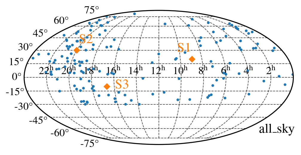
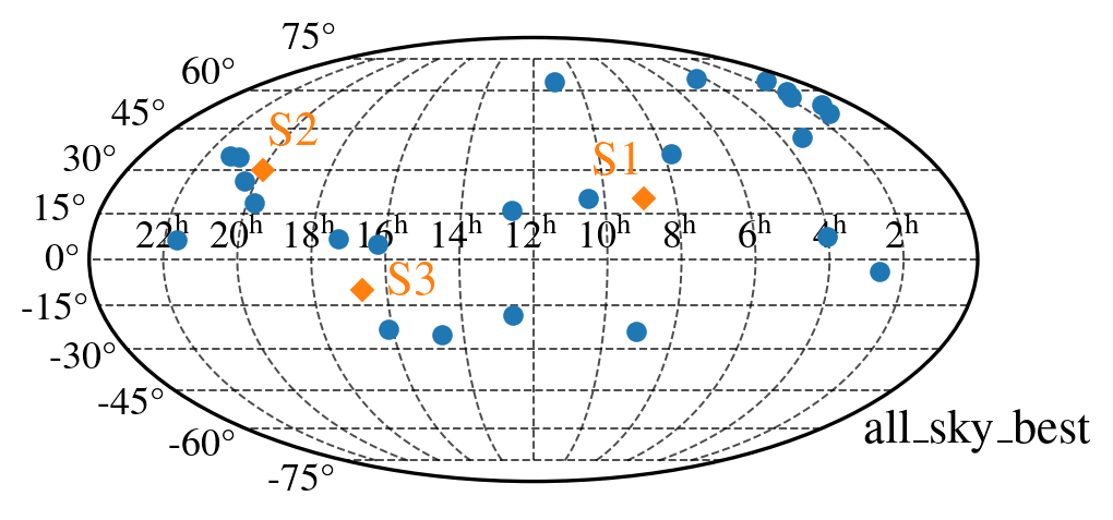
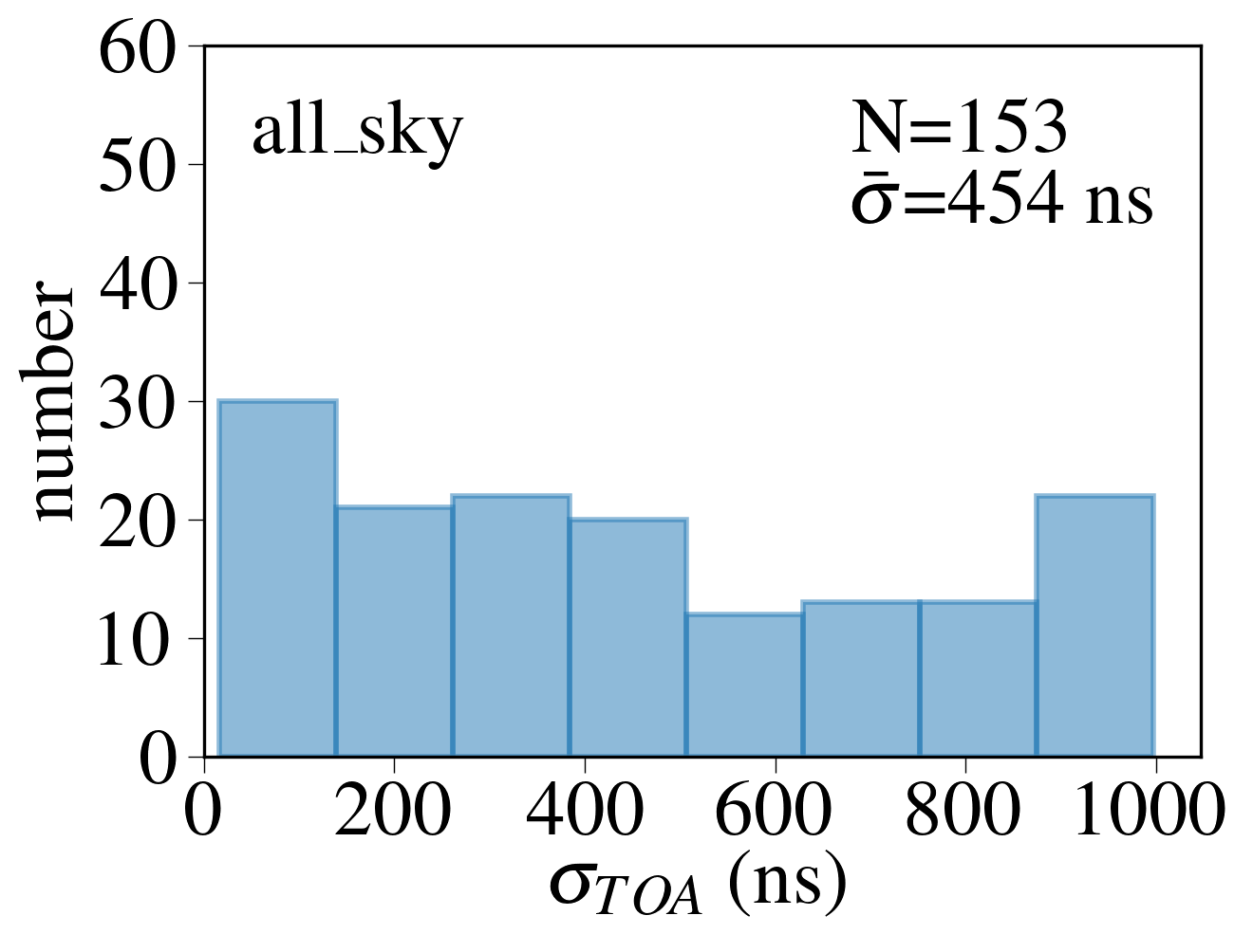
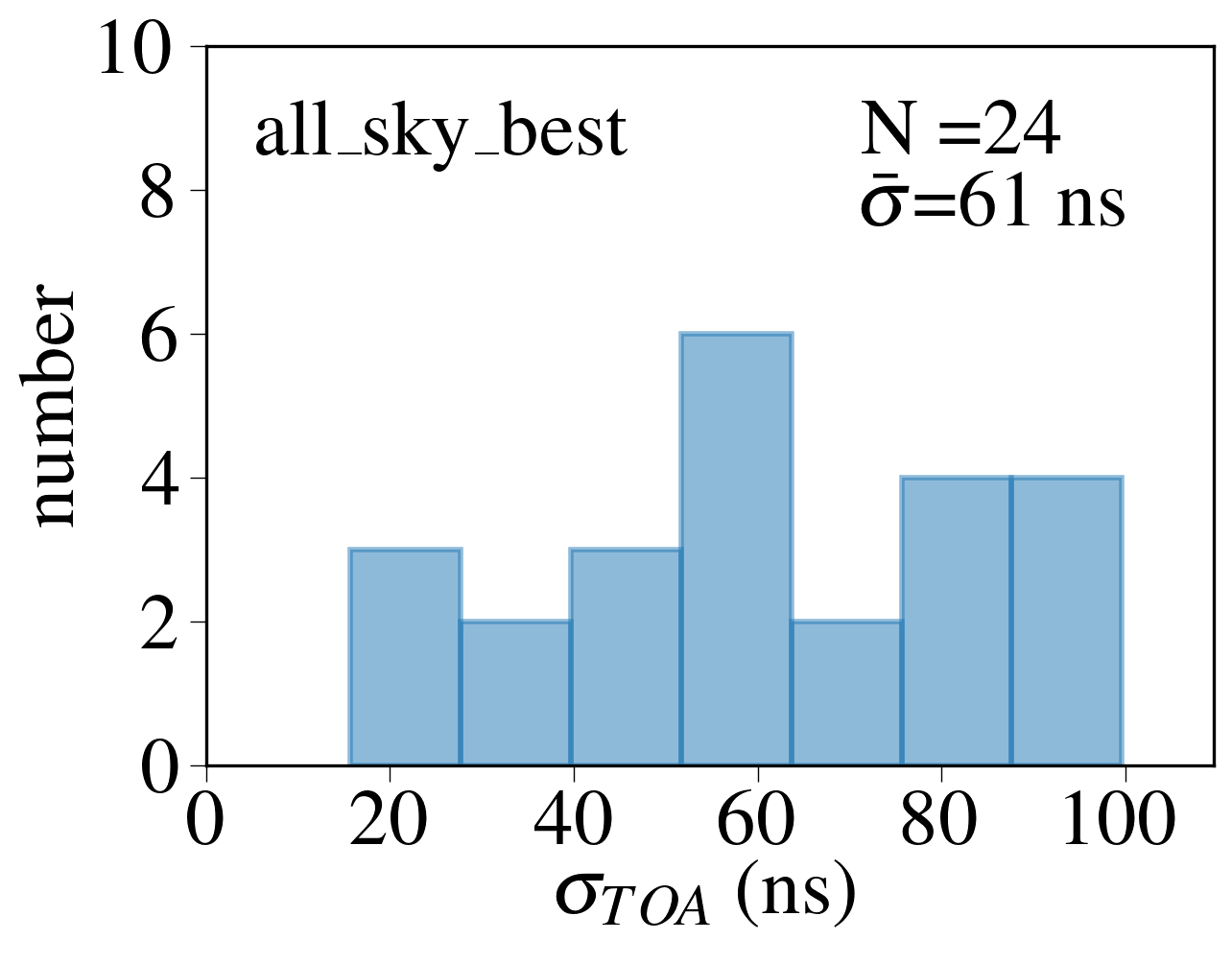
which is a function of pulsar spin period , pulse duty cycle , and integration time . is the systematic error due to chromatic variations in pulse width caused by interstellar scattering and dispersion. is the uncertainty in DM estimation between two frequency channels. contains uncertainties due to radio frequency interference, incorrect gain calibration, and instrumental self-polarization. NANOGrav considers to be the minimum criterion for inclusion of an MSP in the PTA, so we adopt that cutoff here. The result are ten mock PTAs with an average of MSPs with . The sky distribution and distribution of for one realization are plotted in the first panel of Figure 1 and the left panel of Figure 2 (all_sky) respectively.
| DM | RA | Dec. | X | Y | Z | ||||||||||||||||||
|---|---|---|---|---|---|---|---|---|---|---|---|---|---|---|---|---|---|---|---|---|---|---|---|
| (ms) | () | () | (ms) | (ms) | (deg) | (deg) | (deg) | (deg) | (mJy) | () | (kpc) | (kpc) | (kpc) | () | () | () | () | () | () | ||||
| 6.64 | 2.19E-21 | 615.09 | 7.42 | 0.80 | -0.39 | 1.85 | 264.39 | -28.29 | 9.11E-04 | 0.08 | -0.91 | -0.06 | -0.67 | 0.30 | -1.00 | -1.00 | -1.00 | -1.00 | 1.09 | 6.50E-04 | -5.60 | 1.00 | |
| 3.19 | 1.86E-19 | 177.42 | 2.01 | 0.06 | 6.82 | -9.80 | 279.87 | -27.63 | 0.004 | 0.15 | -2.08 | 0.69 | 2.77 | -1.00 | 1757.16 | 0.01 | 1757.16 | 5.68 | 0.05 | 0.09 | -5.60 | 1.00 | |
| 3.27 | 9.73E-21 | 336.38 | 3.86 | 0.11 | -15.20 | -7.19 | 264.06 | -45.61 | 0.002 | 0.33 | -2.45 | -3.79 | -5.45 | -1.82 | -2.00 | -2.00 | -2.00 | -2.00 | 0.11 | 0.02 | -5.60 | 1.00 | |
| 4.42 | 1.37E-19 | 112.95 | 0.00 | 0.48 | 33.95 | 15.35 | 269.57 | 7.82 | 8.00E-04 | 0.03 | -2.70 | 3.37 | 3.49 | 1.66 | -1.00 | -1.00 | -1.00 | -1.00 | 0.53 | 0.02 | -5.60 | 1.00 | |
| 14.04 | 4.74E-21 | 638.35 | 10.42 | 0.50 | -3.47 | 0.52 | 263.76 | -31.60 | 0.012 | 0.71 | -3.04 | -0.46 | 0.89 | 0.07 | -2.00 | -2.00 | -2.00 | -2.00 | 1.00 | 8.17E-04 | -5.60 | 1.00 | |
| 25.52 | 7.16E-20 | 1415.46 | 1143.50 | 0.79 | 12.99 | -0.46 | 273.89 | -17.89 | 2.26E-04 | 0.08 | -0.18 | 4.35 | -10.36 | -0.16 | -1.00 | -1.00 | -1.00 | -1.00 | 2.12 | 1.95E-04 | -5.60 | 1.00 | |
| 7.00 | 7.94E-21 | 552.88 | 1514.56 | 0.21 | 54.88 | 0.25 | 293.04 | 19.55 | 2.54E-06 | 7.14E-04 | -2.13 | 13.71 | -1.14 | 0.07 | -1.00 | -1.00 | -1.00 | -1.00 | 0.29 | 0.00 | -5.60 | 1.00 | |
| 14.44 | 2.79E-19 | 943.11 | 500.37 | 0.29 | -43.43 | -0.23 | 221.07 | -60.08 | 0.002 | 0.54 | -1.69 | -10.41 | -2.50 | -0.06 | -2.00 | -2.00 | -2.00 | -2.00 | 0.58 | 0.02 | -5.60 | 1.00 | |
| 28.56 | 5.91E-21 | 215.86 | 0.04 | 1.29 | 4.94 | 10.38 | 259.74 | -19.19 | 0.006 | 0.52 | -0.80 | 0.78 | -0.54 | 1.66 | 101.11 | 0.04 | 101.11 | 27.34 | 3.62 | 3.04E-04 | -5.60 | 1.00 | |
| 1.98 | 6.71E-21 | 372.40 | 1.68 | 0.34 | -2.35 | 4.21 | 260.91 | -28.64 | 0.002 | 0.16 | -0.64 | -0.35 | 0.07 | 0.62 | -1.00 | -1.00 | -1.00 | -1.00 | 0.25 | 0.01 | -5.60 | 1.00 |
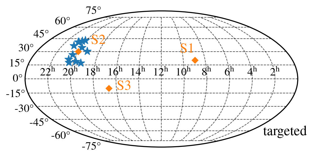
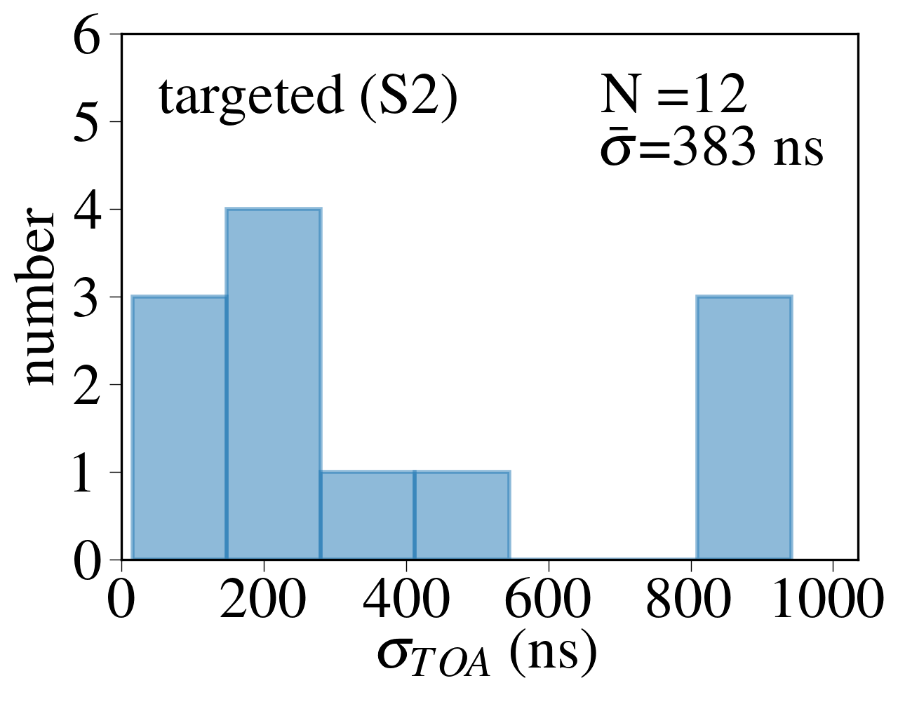
Next, we consider two variants of our mock timing program: (1) an all-sky PTA consisting of only pulsars with ns (all_sky_best) and (2) a targeted campaign in an area of the sky consisting of pulsars within a radius, where the GW source is chosen to be located within that sky area (targeted). Since the antenna pattern functions increase with a closer (but not perfect) alignment between the source and the pulsar (see the definitions in Ellis et al. 2012), a PTA campaign which targets pulsars near an EM-selected source may be more advantageous for detecting its GW signal. We plot the pulsars in one realization of all_sky_best as large filled circles in the second panel of Figure 1, and those in targeted as stars in the third panel. Their respective distributions are shown in the last two panels in Figure 2. The properties of a sample of simulated MSPs are shown in Table 1, and ten realizations of the mock population are available in machine-readable form online.
Then, for each pulsar sample in each realization, we construct mock PTA observations which have the baseline of years which is approximately the length of the current PTAs. The cadence of observations is chosen to be either monthly or weekly, to imitate the current “monthly” and “high cadence” campaigns of NANOGrav (Alam et al., 2021a).
| Source | R.A. | decl. | ||||
|---|---|---|---|---|---|---|
| deg | deg | Hz | Mpc | ns | ||
| S1 | 133.7036 | 20.1085 | 9 | 8.28 | 3.2 | 3.4 |
| S2 | 300 | 30 | 9 | 8 | 2.5 | 13.9 |
| S3 | 250 | 10 | 9 | 8 | 2.5 | 13.9 |
| Source | PTA | Campaign |
|---|---|---|
| S1 | all_sky | 15 yr, monthly |
| all_sky_best | 15 yr, monthly | |
| all_sky_best | 15 yr, weekly | |
| S2 | all_sky | 15 yr, monthly |
| all_sky_best | 15 yr, monthly | |
| all_sky_best | 15 yr, weekly | |
| targeted | 15 yr, monthly | |
| targeted | 15 yr, weekly | |
| S3 | all_sky | 15 yr, monthly |
| all_sky_best | 15 yr, monthly | |
| all_sky_best | 15 yr, weekly |
2.2 Parameters and GW signals of an SMBHB
We consider a binary system with component masses and . The so-called chirp mass is given by . We assume the system is in a circular orbit whose GW frequency is related to its orbital frequency and is often expressed as . The source is located at a luminosity distance ; since in this work we will only consider nearby sources, we ignore the effect of redshift: . For simplicity, we only consider the “Earth term” in the timing residual and do not consider the “pulsar term,”555Our justification for only considering the Earth term is mainly twofold: (1) our methodology (see §2.3) is only concerned with the parameter measurement uncertainty and does not inform the possible bias in the posterior distribution introduced by dropping the pulsar term; (2) extracting source information from the pulsar term would require precise measurements of the pulsar distance which we do not assume in this work. and hence only the combination can be constrained. It is often convenient to redefine the amplitude as .
The sky position of the source is written as polar and azimuthal angles and (corresponding to right ascension and declination in units of radians: , ). We assume the frequency evolution of the binary over the course of years is negligible (i.e., a monochromatic signal). We further assume the BHs are non-spinning, since PTAs are largely insensitive to the effects of spin in an SMBHB system (see Sesana & Vecchio 2010).
Such a binary system is then described by the following parameters: , where are the inclination, GW polarization angle, and initial orbital phase, respectively. For simplicity, we adopt fixed values , and an intermediate inclination for each of the sources, since these are less astrophysical interesting parameters for our study. We then follow the usual definitions in Ellis et al. (2012) and Aggarwal et al. (2019) to compute the Earth-term timing residual Res corresponding to each pulsar which has coordinate and .
The first source (S1) which will be “observed” by our mock PTA is the circular and non-spinning analog of the well-known SMBHB candidate OJ 287 (e.g., Sillanpaa et al. 1988; Lehto & Valtonen 1996; see e.g., Dey et al. 2019; Valtonen et al. 2021 for a recent review). Adopting the binary parameters in Dey et al. (2018), we estimate a GW amplitude ns. We note that while it is possible to compute a more accurate waveform for this complex binary candidate (see e.g., Valtonen et al. 2021), in this work we only seek to obtain estimates of its detection and parameter measurement prospects.
As can be seen in Figure 1, S1 is located in an area of the sky where few mock pulsars are nearby (e.g. within a 10 deg radius), thereby making a future targeted pulsar timing campaign with DSA-2000 unlikely. Prompted by this, we consider a mock source (S2) which (1) has similar binary parameters but is located at the part of the sky where it may be observed by a targeted campaign and (2) represents a generic SMBHB candidate, whereas S1 is based on an actual candidate. We additionally consider an S3, who shares the same binary parameters as S2 but is at a less advantageous location for pulsar searching and timing (and hence the possibility of a targeted campaign). On the other hand, it is located outside the Galactic plane and suffers from less reddening and extinction effects. Thus, S3 represents sources which could be easily detected or observed by most EM observatories. The parameters of the three sources are listed in Table 2, where the S1 parameters are based on Dey et al. (2018).
To summarize, we observe the three sources with two all-sky PTAs with either weekly or monthly cadence over 15 years. However, an all_sky campaign at a weekly cadence is not under consideration here since the total observing time would exceed the 25% available for pulsar timing. For S2, we additionally consider a targeted campaign at both cadences. Those mock programs are also summarized in Table 3.
2.3 Estimating binary parameters using the Fisher matrix formalism
The Fisher matrix is often used to assess the parameter estimation performance of an experiment in fields such as cosmology (e.g., Albrecht et al. 2006) and GW astrophysics (e.g., Sesana & Vecchio 2010; McGrath & Creighton 2021). While it can lead to a less accurate prediction of the performance of the experiment (see e.g., Vallisneri 2008) than the mock data analysis approach, it is significantly less computationally expensive and thus can be applied to a large number of experimental setups and realizations. In this section, we describe how we apply the Fisher matrix formalism to predict the prospects of mock PTAs as described in §2.1 of measuring the parameters of the three SMBHBs as depicted in §2.2.
We begin by first computing the Fisher matrix for each pulsar (indexed by ):
where and are the indices for binary parameters, denotes each observation, represents the of the -th pulsar as discussed in §2.1666We have assumed white noise for the Fisher matrix formalism. Properly including pulsar red noise would require non-trivial modifications to the Fisher matrix, which is beyond the scope of this paper. However, for a discussion of the potential effect of red noise on detection and parameter estimation, see Section 3.4., and is the Earth-term timing residual corresponding to the -th pulsar as described in §2.2. Here we fix the values of and to mimic the search for a CW signal where the source has been pinpointed (which is a reasonable assumption if the candidate is identified electromagnetically), which means we do not compute the partial derivatives with respect to or , and hence which correspond to the parameters .
We then compute the Fisher matrix for multiple pulsars at various locations {, } (i.e., a PTA) by summing the matrices:
Instead of directly inverting the matrix , we first ensure it is well-conditioned, by normalizing the matrix by the factor so that the diagonal elements are 1 and the off-diagonal elements are of order unity. We then use singular value decomposition to invert the normalized matrix: . We then divide by the normalization factor to obtain the final covariance matrix , where . Finally, we check the accuracy of the inversion by multiplying the covariance matrix by the original Fisher matrix and confirm that its difference from the identity matrix is lower than an error threshold: max(. We can then obtain the measurement uncertainty of parameter from the -th diagonal element . In this work, we focus on the uncertainties of the two more astrophysically interesting parameters, and .
Finally, we estimate the total SNR by summing the contribution from each pulsar: = SNR, where SNRa = . In this work, we focus our analysis in the strong signal regime (defined in this work as SNR) so that , instead of being an lower limit, approaches the actual measurement uncertainty. Therefore we only record the value of if SNR is greater than 5 in a realization.
3 Results
3.1 PTA observations of an OJ 287-like binary candidate
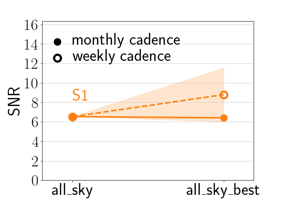
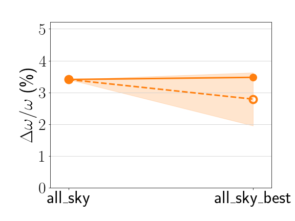
We first investigate whether S1 can be observed by a future all-sky PTA at a either weekly or monthly cadence, i.e. our simulated all_sky and all_sky_best, by performing Fisher matrix analysis for each simulated PTA. At a monthly cadence, only 2/10 of the realizations of an all_sky PTA exceed our SNR threshold of 5. Their SNRs slightly decrease in all_sky_best, which is expected because the pulsars in all_sky_best are a subset of the ones in all_sky (solid line in Figure 3). If only the best pulsars (all_sky_best) are monitored at a weekly cadence, 9/10 of the realizations have SNR, and the mean value increases to (dashed line).
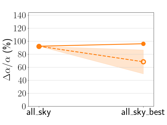
We proceed to compare the measurement uncertainties between GW- and EM-based methods, where the GW-based uncertainties are computed using the Fisher matrix method in §2.3, and the EM-based uncertainties are based on the reported uncertainties of , , and from Dey et al. (2018). The measurement uncertainty of the GW amplitude (quantified by ) is at the level (middle panel), far exceeding the EM-based measurement uncertainty of for this binary candidate. By contrast, can be constrained at the few percent level despite the modest SNR (right panel); it is however still greater than the EM-based uncertainty of .
Thus, we tentatively conclude that a future PTA with DSA-2000 which resembles our all_sky or all_sky_best could detect the GW signal from OJ 287 with years of data at monthly cadence. However, evidence for its binarity based only on GW observations will be modest, unless GW data (especially the more precise measurement of ) are interpreted alongside EM observations. Further, the stochastic GWB has a fiducial power-law spectral shape which increases in amplitude at low GW frequencies; therefore the GWB would have a significant effect on the detectability of sources emitting at (particularly) lower frequencies. See Section 3.4 for a discussion of this effect on the three mock sources considered in this paper.
It is worth noting that the all_sky campaign only increases the SNR by compared to all_sky_best, despite monitoring times the number of pulsars. This suggests that if the total number of observations is a limited resource, it may be best spent on the highest quality pulsars, either at the same cadence or a higher cadence. We explore this further in the following sections.
3.2 PTA observations of a mock binary candidate
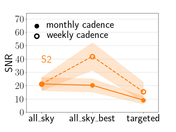
In this section, we consider the detectability and parameter measurement uncertainties of the mock source S2, which has a larger GW amplitude ( ns) and is located in a part of the sky where more pulsars may be found and monitored. We first compute the expected results of a monthly, 15 yr-long campaign. As we show in the left panel of Figure 4, the highest SNR is reached in the all_sky campaign; it decreases in all_sky_best and decreases further in targeted. This can be understood by the fact that targeted has comparable pulsar timing noise as all_sky, but times fewer pulsars in the array. Similarly, all_sky_best has much fewer pulsars than all_sky and hence a lower SNR, despite a higher median pulsar timing quality.
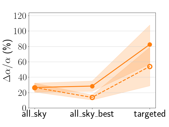
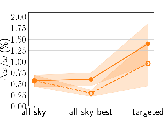
As we also show in the last two panels of Figure 4, targeted results in poorer constraints on and , consistent with its lowest SNR. Nonetheless, these GW-based parameter measurements are better than the constraints obtained from typical EM observations for the following reasons. (Recall that S2 represents a generic EM binary candidate and therefore its parameters are assumed to be measured from standard methods.) First, an observed variability period caused by modulated accretion in the binary may not directly correspond to its intrinsic orbital period, since this relationship may be mass ratio-dependent and the observed period may be at a few times the orbital period (see e.g., D’Orazio et al. 2013; Farris et al. 2014; Noble et al. 2021); therefore, an EM-based frequency measurement would have an (underestimated) uncertainty of , which is orders of magnitude larger than the GW-basement measurement (right panel in Figure 4). Second, standard BH mass measurements suffer from a systematic uncertainty of dex (e.g., Shen 2013); combined with the aforementioned uncertainty on , this translates to a of approximately 120%, which is a few times higher than the GW-based measurement (middle panel in Figure 4). These precise GW parameter measurements can allow meaningful comparisons with EM-based measurements as a robust test of the binary model, breaking the degeneracies arising from EM-only observations, and testing the predictions of SMBHB theory.
It is however important to note that all_sky boasts the highest SNR simply due to the fact that it is timing times more pulsars (than all_sky_best) and that the contribution of bottom 85% of the pulsars to the SNR combined only increases the SNR by . Therefore it would be interesting to investigate whether all_sky_best or targeted is a more efficient approach to achieve a similar scientific outcome.
To do so, we compare the results of the high-cadence, weekly all_sky_best and targeted campaigns with the (monthly) all_sky campaign. As shown in Figure 4, we predict that all_sky_best results in the highest SNR and best parameter measurements; this is despite the fact that all_sky_best costs 40% less total telescope time than all_sky. Likewise, a high-cadence targeted campaign requires only a third of the time as all_sky, but achieves a similar SNR. Furthermore, both high-cadence campaigns can measure and at precise levels which are better than the typical EM measurements as discussed previously. Therefore, we conclude that all_sky_best and targeted are both possible, if not preferable, alternatives to all_sky.
3.3 PTA observations of a second mock binary candidate
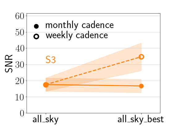
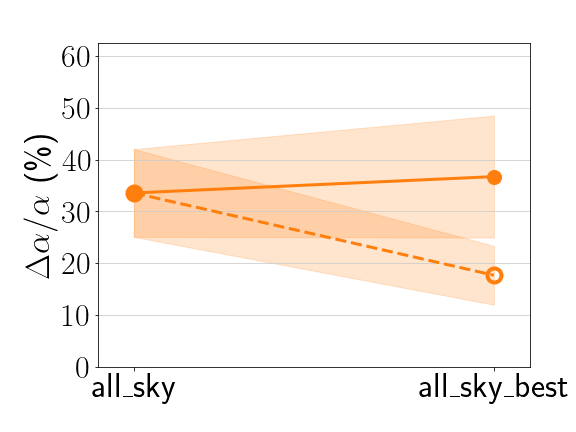
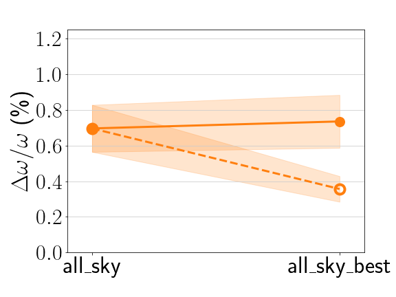
Finally, we examine the detection and parameter estimation prospects of S3. As we show in Figure 5, the expected outcome of all_sky and all_sky_best follows the same trend; namely, all_sky results in a higher SNR for the same cadence, but the high-cadence all_sky_best campaign outperforms all_sky at a lower cost of total telescope time. Further, despite the slightly lower SNR than S2 (consistent with the difference in sky location), the parameters of S3 can still be measured to moderate to high precision.
As discussed earlier, the sky location of S3 may be more representative of that of a likely EM candidate: it is located where it is more likely to be found by EM observatories, including all-sky surveys; on the other hand, it is not at such a fortuitous location that it happens to be in close proximity to a large number of (high quality) MSPs. Fortunately, its detection prospects are nonetheless good in both all-sky campaigns and are only mildly impacted by its “inferior” location. This suggests that, contrary to conventional wisdom, dedicated timing campaigns targeting pulsars near likely sources may not be necessary, efficient, or possible for CW observations.
3.4 Effects of the GWB and pulsar red noise on the detectability of S1–S3
Recently, a red noise process which has a common spectrum across pulsars has been observed in the regional PTAs and the combined International Pulsar Timing Array dataset (Arzoumanian et al., 2020; Chen et al., 2021; Goncharov et al., 2021; Antoniadis et al., 2022). While the PTAs have not confirmed this common red noise process as the GWB, it already needs to be accounted for in more recent CW searches (e.g. NANOGrav Collaboration, in prep.) and will have an effect on PTA’s sensitivity to CWs, especially at lower frequencies. Further, some level of red noise is present in many, if not most, MSPs, which would further compromise the observability of CW sources.
While our Fisher matrix methodology does not handle red noise, in this section, we seek to understand the potential effect of the GWB and pulsar red noise on the detectability of CW sources using simulated PTA sensitivity curves and speculate their implications for binary parameter estimation.
The GWB has a power law power spectrum in the form:
where we adopt the median value of the amplitude from the NANOGrav 12.5 yr analysis: (Arzoumanian et al., 2020), and (Phinney, 2001).
The power spectrum of the pulsar red noise is given by (e.g., Alam et al. 2021b):
where and are the amplitude and the index, respectively. We simulate and for each mock pulsar using the model developed by Shannon & Cordes (2010). They determined that the natural log of the measured, red timing noise after a second-order polynomial fit is normally distributed as . is the post-fit red noise scaled to the spin period and period derivative given by
| (1) |
where , , and are estimated over the pulsar population and is the timescale of the residuals in years. We assume that spin period derivatives are uncorrelated with spin period and are distributed log-normally with and . We adopt the updated values for , , , , and , estimated for a larger sample of MSP red noise measurements, in Table 4 of Lam et al. (2017), row “.” The red noise index, , is assumed to be -5.6 for all MSPs. By combining Equation 1 and Equation 15 of Lam et al. (2017) for the measured red noise in terms of and , we can directly draw for each model pulsar where
and
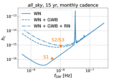
To simulate the PTA sensitivity to CWs in the presence of these noise terms, we use the software package hasasia777https://github.com/Hazboun6/hasasia (Hazboun et al., 2019). We first compute the sensitivity curve by using the sky positions of simulated all_sky pulsars and only including white timing noise (see §2.1). Following the previous sections, we assume a 15-yr PTA with a monthly cadence. The resulting sensitivity is shown as the solid curve in Figure 6. For a monochromatic source (which we assume throughout the paper) emitting at with a strain amplitude , the expected SNR is , where is the effective strain-noise power spectral density for the PTA and is related to the sensitivity curve: (Hazboun et al., 2019). Therefore, the resulting SNRs for S1 and S2/S3 are 2.2 and 9.3, respectively, consistent with our results in §3 that the sources are detectable at the intermediate to high SNR level at monthly cadence.888Note however that the sensitivity curve is averaged over the sky and is not directly applicable to targeted searches. Therefore, the sensitivity curves in Figure 6 are meant for comparison with each other for the purpose of understanding the effect of red noise.
Next, we recompute the sensitivity in the presence of the GWB. The result is shown as the dashed curve. As expected, the GWB severely decreases the PTA sensitivity to CWs, especially at frequencies lower than Hz where it decreases by up to an order of magnitude. Consequently, S1 would not be detectable above the GWB (SNR=0.2), while S2 and S3 may still be detectable, albeit with a lower SNR (2.7).
Finally, we include the pulsar red noise and show the resulting sensitivity curve as the dash-dotted curve. The effect is less pronounced, with the sensitivity decreasing by less than a factor of a few at all frequencies, resulting in an SNR = 0.2 (2.1) for S1 (S2/S3).
We further anticipate that PTA’s ability to estimate binary parameters would also decrease in the presence of red noise. This is based on the fact that at a given frequency, source detectability and parameter measurability closely track each other (see Figures 3 – 5), i.e., a lower SNR corresponds to a larger measurement uncertainty.
While our Fisher matrix method cannot handle red noise and hence our conclusions in this work regarding source detectability and observing strategies are drawn assuming only white noise (i.e., solid curve in Figure 6), future work would be able to make more accurate predictions of the detectability of CW sources by taking into account the additional noise, especially the GWB. In practice, the (relatively small) effect of pulsar red noise could be mitigated by only including pulsars with low red noise levels in the PTA, while the effect of the astrophysical GWB cannot removed.
4 Summary and Conclusions
In this work, we have applied the Fisher matrix formalism to predict the SMBHB parameter estimation prospects of a future PTA with DSA-2000. We focus on the case where the sky location of the source is known via the prior identification of a possible EM counterpart, motivated by (1) the boosted detection SNR and parameter measurements by searching for the GW signal at a fixed sky location, and (2) the possibility of studying SMBHBs in a true multi-messenger fashion. Compared to previous work, we have taken a more realistic approach, taking into consideration factors such as practical and observational constraints of a PTA, the Galactic pulsar population, the number and timing precision of MSPs detectable by a telescope, and their spatial distribution.
As a case study, we first examined the detection prospects of the well-known SMBHB candidate OJ 287 (using S1 as a surrogate). We estimate that a future PTA with DSA-2000 may be able to detect the source with 15 years of data (assuming only pulsar white noise). While the measurement uncertainty of the GW amplitude is large, which translates to a poor constraint on the system mass, the PTA constraint on the GW frequency is at a level which is more comparable to the EM equivalent, permitting the possibility of robustly testing its binary model through a joint interpretation of GW and EM data.
We then generalized this approach to a mock source, and our main results can be summarized as follows:
-
1.
We have considered three types of PTAs, an all-sky PTA which observes all pulsars in our mock pulsar sample (all_sky), an all-sky PTA which only observes the best quality pulsars (all_sky_best), and a PTA which targets pulsars near an EM-selected binary candidate (targeted). At equal observing cadence, all_sky naturally results in the highest SNR and best parameter measurements. However, even with less total observing time, the high-cadence all_sky_best outperforms the other ones.
-
2.
We have examined the detection and parameter estimation prospects of the mock source placed at different sky locations. If it is at a fortuitous location where a higher-cadence targeted campaign is possible (i.e., S2), the targeted campaign yields results similar to a lower-cadence all_sky campaign. More realistic is a sky location where targeted is not feasible due to the dearth of pulsars near the source (i.e., S3); this scenario may be more likely for EM-selected binary candidates. Fortunately, at such a location, its detection prospects with all_sky or all_sky_best may only decrease slightly compared to S2.
-
3.
For a more typical EM candidate (represented by S2 and S3), the GW amplitude and frequency parameters may be constrained at a level which is better than standard EM measurements. Particularly, GW frequency can be easily constrained within a few percent; this level of precision is consistent with similar estimates from previous work using both mock data analysis (e.g., Liu & Vigeland 2021) and Fisher matrix-based approaches (e.g., Sesana & Vecchio 2010).
Those results suggest the following strategies for a PTA to achieve the best science outcome at the lowest cost:
-
1.
Ideally, an all-sky PTA timing all pulsars detectable by pulsar surveys at a high cadence yields the best outcome. In reality, such a PTA costs more time than what is available on a single telescope or array. A PTA which only times the best pulsars can achieve similar results at a lower cost of total telescope time, even if observing at a higher cadence.
-
2.
Applying the principle of choosing quality over quantity, an upgraded and downsized version of the present-day PTAs would be capable of detecting EM-selected SMBHBs with a variety of source parameters and measuring their parameters at precision levels which are better than conventional EM measurements. Such a PTA can operate as a true GW observatory of SMBHBs and complement EM searches and observations with profound implications for the multi-messenger studies of SMBHBs.
-
3.
A dedicated PTA which targets a small number of MSPs near the EM-selected candidate may not be feasible, since the sky locations where MSPs can be found and where EM binary candidates may be observed likely do not coincide. Fortunately, this may not be necessary either, because an all-sky PTA consisting of a small number of high quality pulsars is capable of observing a source at any location with good results.
We end with a caveat about our preference for all_sky_best over all_sky. We have assumed known sky locations and therefore have not considered the PTA measurement uncertainties of and in this work. However, it has been known that sky localization improves with the number pulsars in the PTA (Sesana & Vecchio, 2010). Therefore, it cannot be determined from our study whether all_sky_best remains the best strategy for an unguided search over the whole sky without an EM counterpart beforehand. It would therefore be interesting to investigate the source localization capability of all_sky_best (with its more realistic pulsar spatial distribution and distribution) and to reexamine its overall single source detection capability.
References
- Aggarwal & Lorimer (2022) Aggarwal, K., & Lorimer, D. R. 2022, On the radio spectra of Galactic millisecond pulsars, arXiv, doi: 10.48550/ARXIV.2203.05560
- Aggarwal et al. (2019) Aggarwal, K., Arzoumanian, Z., Baker, P. T., et al. 2019, ApJ, 880, 116, doi: 10.3847/1538-4357/ab2236
- Alam et al. (2021a) Alam, M. F., Arzoumanian, Z., Baker, P. T., et al. 2021a, ApJS, 252, 4, doi: 10.3847/1538-4365/abc6a0
- Alam et al. (2021b) —. 2021b, ApJS, 252, 4, doi: 10.3847/1538-4365/abc6a0
- Albrecht et al. (2006) Albrecht, A., Bernstein, G., Cahn, R., et al. 2006, arXiv e-prints, astro. https://arxiv.org/abs/astro-ph/0609591
- Amaro-Seoane et al. (2017) Amaro-Seoane, P., Audley, H., Babak, S., et al. 2017, arXiv e-prints, arXiv:1702.00786. https://arxiv.org/abs/1702.00786
- Antoniadis et al. (2022) Antoniadis, J., Arzoumanian, Z., Babak, S., et al. 2022, MNRAS, 510, 4873, doi: 10.1093/mnras/stab3418
- Arzoumanian et al. (2018) Arzoumanian, Z., Brazier, A., Burke-Spolaor, S., et al. 2018, The Astrophysical Journal Supplement Series, 235, 37, doi: 10.3847/1538-4365/aab5b0
- Arzoumanian et al. (2020) Arzoumanian, Z., Baker, P. T., Blumer, H., et al. 2020, ApJ, 905, L34, doi: 10.3847/2041-8213/abd401
- Astropy Collaboration et al. (2018) Astropy Collaboration, Price-Whelan, A. M., Sipőcz, B. M., et al. 2018, AJ, 156, 123, doi: 10.3847/1538-3881/aabc4f
- Bates et al. (2014) Bates, S. D., Lorimer, D. R., Rane, A., & Swiggum, J. 2014, MNRAS, 439, 2893, doi: 10.1093/mnras/stu157
- Burt et al. (2011) Burt, B. J., Lommen, A. N., & Finn, L. S. 2011, ApJ, 730, 17, doi: 10.1088/0004-637X/730/1/17
- Charisi et al. (2016) Charisi, M., Bartos, I., Haiman, Z., et al. 2016, MNRAS, 463, 2145, doi: 10.1093/mnras/stw1838
- Chen et al. (2021) Chen, S., Caballero, R. N., Guo, Y. J., et al. 2021, MNRAS, 508, 4970, doi: 10.1093/mnras/stab2833
- Christy et al. (2014) Christy, B., Anella, R., Lommen, A., et al. 2014, ApJ, 794, 163, doi: 10.1088/0004-637X/794/2/163
- Cordes & Lazio (2002) Cordes, J. M., & Lazio, T. J. W. 2002, arXiv e-prints, astro. https://arxiv.org/abs/astro-ph/0207156
- Dey et al. (2018) Dey, L., Valtonen, M. J., Gopakumar, A., et al. 2018, ApJ, 866, 11, doi: 10.3847/1538-4357/aadd95
- Dey et al. (2019) Dey, L., Gopakumar, A., Valtonen, M., et al. 2019, Universe, 5, 108, doi: 10.3390/universe5050108
- D’Orazio & Di Stefano (2018) D’Orazio, D. J., & Di Stefano, R. 2018, MNRAS, 474, 2975, doi: 10.1093/mnras/stx2936
- D’Orazio et al. (2013) D’Orazio, D. J., Haiman, Z., & MacFadyen, A. 2013, MNRAS, 436, 2997, doi: 10.1093/mnras/stt1787
- D’Orazio et al. (2015) D’Orazio, D. J., Haiman, Z., & Schiminovich, D. 2015, Nature, 525, 351, doi: 10.1038/nature15262
- Ellis et al. (2012) Ellis, J. A., Siemens, X., & Creighton, J. D. E. 2012, ApJ, 756, 175, doi: 10.1088/0004-637X/756/2/175
- Farris et al. (2014) Farris, B. D., Duffell, P., MacFadyen, A. I., & Haiman, Z. 2014, ApJ, 783, 134, doi: 10.1088/0004-637X/783/2/134
- Faucher-Giguère & Kaspi (2006) Faucher-Giguère, C., & Kaspi, V. 2006, ApJ, 643, 332, doi: 10.1086/501516
- Foord et al. (2017) Foord, A., Gültekin, K., Reynolds, M., et al. 2017, ApJ, 851, 106, doi: 10.3847/1538-4357/aa9a39
- Goncharov et al. (2021) Goncharov, B., Shannon, R. M., Reardon, D. J., et al. 2021, ApJ, 917, L19, doi: 10.3847/2041-8213/ac17f4
- Graham et al. (2015a) Graham, M. J., Djorgovski, S. G., Stern, D., et al. 2015a, Nature, 518, 74, doi: 10.1038/nature14143
- Graham et al. (2015b) —. 2015b, MNRAS, 453, 1562, doi: 10.1093/mnras/stv1726
- Guo et al. (2020) Guo, H., Liu, X., Zafar, T., & Liao, W.-T. 2020, MNRAS, 492, 2910, doi: 10.1093/mnras/stz3566
- Hallinan et al. (2019) Hallinan, G., Ravi, V., Weinreb, S., et al. 2019, in Bulletin of the American Astronomical Society, Vol. 51, 255. https://arxiv.org/abs/1907.07648
- Hazboun et al. (2019) Hazboun, J. S., Romano, J. D., & Smith, T. L. 2019, Phys. Rev. D, 100, 104028, doi: 10.1103/PhysRevD.100.104028
- Hobbs (2013) Hobbs, G. 2013, Classical and Quantum Gravity, 30, 224007, doi: 10.1088/0264-9381/30/22/224007
- Hunter (2007) Hunter, J. D. 2007, Computing in Science & Engineering, 9, 90, doi: 10.1109/MCSE.2007.55
- Ivezic et al. (2008) Ivezic, Z., Tyson, J. A., Abel, B., et al. 2008, ArXiv e-prints. https://arxiv.org/abs/0805.2366
- Kelley et al. (2017) Kelley, L. Z., Blecha, L., Hernquist, L., Sesana, A., & Taylor, S. R. 2017, MNRAS, 471, 4508, doi: 10.1093/mnras/stx1638
- Kelley et al. (2018) —. 2018, MNRAS, 477, 964, doi: 10.1093/mnras/sty689
- Kelley et al. (2021) Kelley, L. Z., D’Orazio, D. J., & Di Stefano, R. 2021, MNRAS, 508, 2524, doi: 10.1093/mnras/stab2776
- Kramer & Champion (2013) Kramer, M., & Champion, D. J. 2013, Classical and Quantum Gravity, 30, 224009, doi: 10.1088/0264-9381/30/22/224009
- Lam et al. (2018) Lam, M. T., McLaughlin, M. A., Cordes, J. M., Chatterjee, S., & Lazio, T. J. W. 2018, ApJ, 861, 12, doi: 10.3847/1538-4357/aac48d
- Lam et al. (2017) Lam, M. T., Cordes, J. M., Chatterjee, S., et al. 2017, ApJ, 834, 35, doi: 10.3847/1538-4357/834/1/35
- Lam et al. (2019) Lam, M. T., McLaughlin, M. A., Arzoumanian, Z., et al. 2019, The Astrophysical Journal, 872, 193, doi: 10.3847/1538-4357/ab01cd
- Lehto & Valtonen (1996) Lehto, H. J., & Valtonen, M. J. 1996, ApJ, 460, 207, doi: 10.1086/176962
- Liu & Vigeland (2021) Liu, T., & Vigeland, S. J. 2021, ApJ, 921, 178, doi: 10.3847/1538-4357/ac1da9
- Liu et al. (2015) Liu, T., Gezari, S., Heinis, S., et al. 2015, ApJ, 803, L16, doi: 10.1088/2041-8205/803/2/L16
- Liu et al. (2016) Liu, T., Gezari, S., Burgett, W., et al. 2016, ApJ, 833, 6, doi: 10.3847/0004-637X/833/1/6
- Liu et al. (2019) Liu, T., Gezari, S., Ayers, M., et al. 2019, ApJ, 884, 36, doi: 10.3847/1538-4357/ab40cb
- Lorimer (2012) Lorimer, D. R. 2012, Proceedings of the International Astronomical Union, 8, 237–242, doi: 10.1017/S1743921312023769
- Manchester et al. (2001) Manchester, R. N., Lyne, A. G., Camilo, F., et al. 2001, MNRAS, 328, 17, doi: 10.1046/j.1365-8711.2001.04751.x
- McGrath & Creighton (2021) McGrath, C., & Creighton, J. 2021, MNRAS, 505, 4531, doi: 10.1093/mnras/stab1417
- McLaughlin (2013) McLaughlin, M. A. 2013, Classical and Quantum Gravity, 30, 224008, doi: 10.1088/0264-9381/30/22/224008
- Noble et al. (2021) Noble, S. C., Krolik, J. H., Campanelli, M., et al. 2021, ApJ, 922, 175, doi: 10.3847/1538-4357/ac2229
- Noble et al. (2012) Noble, S. C., Mundim, B. C., Nakano, H., et al. 2012, ApJ, 755, 51, doi: 10.1088/0004-637X/755/1/51
- Phinney (2001) Phinney, E. S. 2001, ArXiv Astrophysics e-prints
- Pol et al. (2021) Pol, N. S., Taylor, S. R., Kelley, L. Z., et al. 2021, ApJ, 911, L34, doi: 10.3847/2041-8213/abf2c9
- Saade et al. (2020) Saade, M. L., Stern, D., Brightman, M., et al. 2020, ApJ, 900, 148, doi: 10.3847/1538-4357/abad31
- Sesana & Vecchio (2010) Sesana, A., & Vecchio, A. 2010, Phys. Rev. D, 81, 104008, doi: 10.1103/PhysRevD.81.104008
- Severgnini et al. (2018) Severgnini, P., Cicone, C., Della Ceca, R., et al. 2018, MNRAS, 479, 3804, doi: 10.1093/mnras/sty1699
- Shannon & Cordes (2010) Shannon, R. M., & Cordes, J. M. 2010, ApJ, 725, 1607, doi: 10.1088/0004-637X/725/2/1607
- Shen (2013) Shen, Y. 2013, Bulletin of the Astronomical Society of India, 41, 61. https://arxiv.org/abs/1302.2643
- Sillanpaa et al. (1988) Sillanpaa, A., Haarala, S., Valtonen, M. J., Sundelius, B., & Byrd, G. G. 1988, ApJ, 325, 628, doi: 10.1086/166033
- Taylor et al. (2016) Taylor, S. R., Vallisneri, M., Ellis, J. A., et al. 2016, ApJ, 819, L6, doi: 10.3847/2041-8205/819/1/L6
- Vallisneri (2008) Vallisneri, M. 2008, Phys. Rev. D, 77, 042001, doi: 10.1103/PhysRevD.77.042001
- Valtonen et al. (2021) Valtonen, M. J., Dey, L., Gopakumar, A., et al. 2021, Galaxies, 10, 1, doi: 10.3390/galaxies10010001