Multipartite entanglement in two-dimensional chiral topological liquids
Abstract
The multipartite entanglement structure for the ground states of two dimensional topological phases is an interesting albeit not well understood question. Utilizing the bulk-boundary correspondence, the calculation of tripartite entanglement in 2d topological phases can be reduced to that of the vertex state, defined by the boundary conditions at the interfaces between spatial regions. In this paper, we use the conformal interface technique to calculate entanglement measures in the vertex state, which include area law terms, corner contributions, and topological pieces, and a possible additional order one contribution. This explains our previous observation of the Markov gap in the 3-vertex state, and generalizes this result to the -vertex state, general rational conformal field theories, and more choices of subsystems. Finally, we support our prediction by numerical evidence, finding precise agreement.
I Introduction
Topologically ordered phases of matter are characterized not by local order parameters but by their pattern of long-range entanglement. Concretely, from the scaling of the entanglement entropy of a bipartition, one can extract a universal property of topological ground states, the so-called topological entanglement entropy [1, 2]. While the topological entanglement entropy provides a signature for topological ground states, it is far from a full characterization of topological data; there are topological states that share the same topological entanglement entropy yet are distinct from each other.
Recent publications [3, 4, 5, 6] initiated the study of multipartite entanglement of topological ground states in two spatial dimensions. In particular, Refs. [3, 4] investigated the recently introduced reflected entropy [7] as well as the entanglement negativity for tripartitions of topological ground states, in which the three spatial subregions meet at junctions. For a system of three spin 1/2 degrees of freedom, the reflected entropy (or more precisely, the Markov gap which is the difference between the reflected entropy and mutual information – see below) detects the tripartite entanglement of the W-state, while it is insensitive to GHZ-type tripartite entanglement [8]. The reflected entropy can thus capture quantum correlations beyond simple Bell or EPR-type bipartite correlations. Indeed, a structure theorem was proven in Ref. [9], classifying the set of states with zero Markov gap 111See Ref. [44] for further discussion that gave the Markov gap its name.. There, the reflected entropy was further studied for gapped as well as critical ground states in one spatial dimension.
Ref. [3] discussed the reflected entropy for two regions and for the integer quantum Hall ground state and the ground state of a two-dimensional chiral -wave superconductor. Here, the total system is put on a spatial sphere and tripartitioned into three regions , , and that meet at two points (junctions). The region is partially traced out to obtain the reduced density matrix for . (For the definition of reflected entropy, see Sec. IV.) By using the bulk-boundary correspondence and techniques from string field theory, Ref. [3] found that the Markov gap, which is the difference between the reflected entropy and the mutual information, is independent of the subregion sizes and given by the universal formula
| (1) |
where is the central charge of the topological liquid, and and for the integer quantum Hall state and chiral -wave superconductor, respectively. On the other hand, Ref. [4] studied the Markov gap for string-net models (the Levin-Wen models), for which the central charge is zero, and found that . (See also Ref. [11].) Equation (1) relates tripartite quantum entanglement to the central charge and hence captures the universal data of topological liquid beyond the topological entanglement entropy. These calculations were done for ideal, representative topological ground states realized deep inside a topological phase. Refs. [3, 4] also numerically studied the reflected entropy in a lattice model of Chern insulators. While the Markov gap was still found to be insensitive to the subregion and systems sizes, the formula (1) does not hold verbatim, but its RHS provides a lower bound of the Markov gap, . Putting these results together, the Markov gap in the tripartition setup above is conjectured to capture the central charge of stable (ungappable) degrees of freedom at the boundary of topological liquid; that is to say, a non-zero Markov gap may be an obstruction to completely gap out the boundary (edge) theory.
Despite these recent results, Eq. (1) has been verified only for a fraction of topological liquids – the Levin-Wen models for non-chiral topological order, and the free fermion models (integer quantum Hall and topological superconductor states). Thus, the majority of interacting chiral topological states with non-zero chiral central charge have not been discussed. Also, the free fermion results are half-numerical; while Ref. [3] analytically constructed the vertex state – an essential ingredient for achieving multipartition in our approach (see Sec. III for details), the relevant entanglement quantities (reflected entropy, Markov gap, entanglement negativity, etc.) had to be computed numerically. Hence, an analytic understanding of the Eq. (1) has been lacking.
In this work, we present an analytical approach to multipartite entanglement that can be applied to generic (chiral) topological ground states in two spatial dimensions. Following Ref. [3], we use the bulk-boundary correspondence and reduce the calculations of the entanglement quantities to calculations in conformal field theory (CFT). Specifically, we will show that the calculations can be reformulated in terms of defect (interface) CFT, and furthermore simplified by taking the advantage the limit of small , where is the bulk gap and is the length of the entangling boundary. By using a series of conformal transformations, a given entanglement quantity can be evaluated as a path integral on a cylinder with topological interfaces.
In addition to reflected entropy and the Markov gap, this approach also allows us to calculate the so-called corner contribution to the bipartite entanglement entropy studied in Refs. [12, 13, 14]. In these works, the subregions for bipartitions containing sharp corners or cusps were considered. It was found that the entanglement entropy receives a geometric angle-dependent contribution. (See also several works on closely-related quantities and setups, such as the charge fluctuations for a subregion with a sharp corner [15, 16], and others [17, 18, 19]. Quantum Hall states on surfaces with cusp singularities were also studied in the literature [20, 21, 22]. As we will see, the corner contribution from our approach, Eq. (32), does not seem to match precisely with the previous works above. We will speculate on the possible source of the discrepancies. Nevertheless, we will show that our prediction (32) agrees with numerically-computed entanglement quantities for four vertex states in the free fermion theory. Here, we extend the construction of three-vertex states (vertex states that can be used to tripartition a topological liquid) in the free fermion theory in Ref. [3] to four vertex states. This allows us to tetrapartition the topological liquid, and test our analytical predictions for the corner contribution and the reflected entropy (Markov gap).
The rest of the paper is organized as follows. In Sec. II, we revisit the calculation of bipartite entanglement entropy for topological ground states in two dimensions using the bulk-boundary correspondence. As is well known, the calculation can be formulated in terms of boundary states in boundary conformal field theory (BCFT). For later use, we reformulate the calculation in terms of defects (interfaces) in CFT and also show that the calculation can be simplified in the limit. In Sec. III, we generalize and extend the approach of Sec. II to multipartitions by considering -vertex states (). This allows us to calculate the corner contribution to bipartite entanglement entropy and the reflected entropy. In Sec. V, we present the construction of four-vertex states and the numerical calculations of entanglement quantities. We conclude with a discussion in Sec. VI.
II Edge theory approach: Review of Bipartite Entanglement Entropy
As noted in the Introduction, our methodology for computing entanglement in chiral topological orders employs the boundary state or “cut-and-glue” approach. This method reduces computations of bulk entanglement quantities to computations of the same quantities in the corresponding edge CFT, for which powerful analytic techniques exist. Indeed, a central technical advance of our work is the use of defect CFT methods to extend the cut-and-glue approach to the computation of the corner contributions as well as multipartite entanglement quantities. In this section, as a warm-up, we review this approach and introduce our defect CFT formalism in the simpler setting of the computation of the bipartite entanglement entropy, for which the result in a chiral topological order is well known.
To that end, let us consider a chiral topological order on the surface of a sphere. We are interested in computing the entanglement entropy for a spatial bipartition of the sphere into two regions and , which we take to be the two hemispheres, such that the entanglement cut lies along the equator. In the cut-and-glue approach to this problem, we physically cut the system along the entanglement cut, giving rise to counter-propagating chiral CFTs along the new edges. We can then “heal” the cut by introducing appropriate tunnelling terms to gap out the CFTs. Now, since the correlation length is effectively zero in the bulk, we may approximate the entanglement between the bulk regions and as arising purely from degrees of freedom near the entanglement cut, namely the gapped edge degrees of freedom. The upshot of the cut-and-glue approach is the reduction of the problem to a computation of the entanglement entropy between the left and right movers in the gapped interface. This approach naturally generalizes to the primary interest of this work, namely a partitioning of a topological phase into three or more spatial subregions, meeting at two junctions. Computations of multipartite entanglement quantities then reduce to computations of the same quantities in a network of multiple gapped interfaces meeting at two junctions, as we will discuss in more detail in Sec. III.
In the remainder of this section, we spell out the computation in the bipartite setting in more detail, with an eye towards setting the stage for the more involved multipartite computations. In particular, for the bipartite case at hand, it is well-established that an appropriate approximation to the ground state of the gapped interface is provided by conformal boundary states known as Ishibashi states [23, 24, 25].
As we shall review below in Sec. II.1, the explicit form of the Ishibashi states are known for generic rational CFTs, allowing for a simple and direct computation of the bipartite entanglement entropy, reproducing the known result for the topological entanglement entropy. Similarly, for a multipartitioning, as described in Ref. [3] and reviewed below in Sec. III, the configuration of gapped interfaces can be approximated by a so-called vertex state. The explicit form of such states for generic rational CFTs is not known, necessitating an alternative approach to computing the entanglement. With this in mind, in Sec. II.2, we introduce a complementary path integral approach to computing the bipartite entanglement entropy, making use of conformal interfaces. Finally, in Sec. II.3, we present an approximation of the preceding path integral, which reduces the computation of the entanglement of a CFT partition function on a torus to one of CFT partition functions on two cylinders. We emphasize that these latter two subsections, while simply reproducing known results for the bipartite entanglement entropy, lay the technical foundations for the subsequent computations of the corner contributions to the bipartite entanglement entropy in Sec. III and the reflected entropy in Sec. IV.
II.1 Boundary states and left-right entanglement entropy
We begin by first reviewing in more detail the CFT description of the interface and the computation of the bipartite entanglement entropy. As noted above, after “gluing” the edges to heal the physical cut along the entanglement cut, the degrees of freedom along the cut may be described by an Ishibashi state.
Formally, Ishibashi states are states satisfying conformal boundary conditions in a non-chiral CFT. Explicitly, let us consider a non-chiral CFT defined on a spatial circle of length . A boundary state is defined to satisfy
| (2) |
where and are the holomorphic and antiholomorphic components of the stress-energy tensor, and is the spatial coordinate [26]. An Ishibashi state satisfies, in addition to (2), similar conditions for conserved currents.
Now, the CFTs describing the edges of chiral topological orders are rational. That is to say, the Hilbert space can be decomposed into a finite number of primary operator sectors labeled by : . The bulk-boundary correspondence states that the anyon in the bulk is associated with a primary operator in the boundary CFT. The chiral sector has orthonormal basis , where is the conformal dimension of the primary operator , is the level that goes from to , and labels the degenerate states in a given level . Similarly, the anti-chiral sector has orthonormal basis , which is isomorphic to . For these rational CFTs, solutions to Eq. (2) are provided by the Ishibashi states, which take the form,
| (3) |
There is a single Ishibashi state for each primary, or anyon, sector . General solutions to the conformal boundary conditions are given by linear combinations of the Ishibashi states. Now, the Ishibashi states are not normalizable. In order to define a physical state, we introduce a regulator and construct the regularized state :
| (4) |
Here is the CFT Hamiltonian , where are zero modes of the stress tensor , is the central charge, and is the length of the entanglement cut. The normalization factor is defined such that these regularized states are orthonormal .
Returning to our problem of computing the entanglement entropy, Ishibashi states were argued to describe the gapped interface along the entanglement cut in Ref. [24]. Indeed, the conformal boundary condition (and the explicit form of the Ishibashi states) pairs up the left and right movers, just as a tunneling interaction would gap out the left and right movers at the interface. The regulator , in this description, is determined by the inverse bulk gap, and hence we will always be interested in the limit. In the context of the bipartition of the sphere, the Ishibashi state thus describes the gapped interface along the entanglement cut when a single anyon line pierces the entanglement cut.
With the description of the interface in hand, we can approximate the entanglement entropy between the bulk regions and as the “left-right” entanglement entropy of the boundary state – that is, the entanglement entropy between the chiral and anti-chiral sectors of the interface Hilbert space. Explicitly, for an interface state of the form , corresponding to the density matrix
| (5) |
describing a superposition of states with single anyon lines threading the entanglement cut, we can explicitly compute the reduced density matrix for the left-movers (or chiral sector),
| (6) |
where the trace is performed over the right-movers (anti-chiral sector). The entanglement entropy is then straightforwardly computed using the replica trick,
| (7) |
Carrying this through, one finds
| (8) |
where the first is the non-universal area law contribution while the second term is the topological entanglement entropy,
| (9) |
where is the quantum dimension of anyon and is the total quantum dimension. For an Ishibashi state , corresponding to a state with a definite anyon line threading the entanglement cut, the topological contribution is . For Abelian topological order, all quantum dimensions and the topological entanglement entropy reduces to , where the second term is the Shannon entropy associated with the probability distribution . We thus see that the boundary state description of the interface captures the expected bipartite entanglement structure of the bulk topological phase.
For the convenience of later discussion, let us also mention a more complicated case of two anyon lines insertion and . The coefficient can be computed as [25]: where is the fusion coefficient. One can show the topological contribution is in the case or 1.
II.2 Conformal interface approach
As described at the beginning of this section, a direct computation of the entanglement entropy from the ground state will not be possible when we later consider multipartitions of the bulk topological phase. While the ground state will satisfy similar conformal boundary conditions as the above Ishibashi states, its explicit form for general CFTs is not known. With this in mind, we now develop an alternative approach to computing the bipartite entanglement entropy using path integral and conformal interface methods [27, 28], which will generalize to the multipartite case. Our strategy will be to re-express the Rényi moments of (reduced) density matrices formed from regularized boundary states as CFT partition functions on closed manifolds with insertions of conformal interfaces through a series of conformal mappings.
First, we start by expressing the density matrix in Eq. (5) as a path integral as depicted pictorially in Fig. 1(a). The top and bottom rows correspond, respectively, to the ket and bra . Focusing first on the ket, the two spacetime sheets correspond to the chiral and anti-chiral sectors of the the theory. The horizontal direction is the spatial direction, of length , with the tildes indicating periodic boundary conditions. The bottom of the path integral denotes the unregularized boundary state . The dashed lines connecting the segments and indicate how the chiral and anti-chiral sectors are glued together as per the conformal boundary condition. The vertical direction denotes imaginary time evolution by , yielding the regularized state . More generally, we can start from a linear superposition , and the Euclidean path integral prepares the regularized state .
Combining these elements yields the glued path integral representation of the ket in the right-most column. Similar considerations hold for the bra, , represented in the second row of the same subfigure. Combining the bra and ket gives the path integral representation of the density matrix . When computing the trace , the top red lines of bra and ket are glued together ( to , to ), and the spacetime manifold becomes a torus.
Now, the computation of entanglement entropy requires computing the Rényi moments of the reduced density matrix, . These quantities can be represented as path integrals with conformal interface insertions, as we now demonstrate. We first take the path integral of , and unfold the boundary state and , as shown in the left of Fig. 1(b). After the unfolding, the doubled sheet of width becomes a single sheet with width . We define the interface operator as the unfolded boundary state :
| (10) |
where the ket of anti-chiral mode is “flipped” to the bra of chiral mode. In other words, is an Ishibashi-type projector on the chiral sector , . Note this is a well-defined projector since is an orthonormal basis in . In general we can consider the linear superposition . Moreover, in the present context, these interfaces are topological, meaning they can be freely deformed in spacetime. Thus, after unfolding, each boundary state () maps to an insertion of the interface operator ().
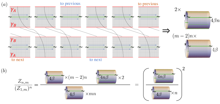
To obtain , we take the path integral of , and glue the red lines for and , as shown in the left of Fig. 1(b) by the black dashed line. Then to obtain , we take copies of path integral of , and glue the red line for of copy to the the red line for of copy , where runs from to . After this gluing, we obtain a torus with circumferences and , and the path integral on this torus is :
| (11) |
The Hamiltonian in this expression is the chiral Hamiltonian 222We treat our BCFT as an interface CFT (ICFT) by the unfolding. Then, the ICFT corresponds to a chiral part of the BCFT.. This is shown in the right of Fig. 1(b). In Fig. 2(a), we show an equivalent path integral representation of where the order of gluing is changed (first glue , then glue and ). In this way, the spacetime path integral can be constructed by gluing annulus amplitudes where each annulus has width and circumference . The closed boundary condition is made explicit in this picture.
The path integral on the torus can be evaluated readily using standard CFT techniques. In CFT, the character of primary field sector is defined as . As a first example, let’s consider the special case of with . can be directly related to the character:
| (12) |
Since by definition, one can read out the normalization factor .
We now compute in the large gap limit of interest . To work in this limit, we need to use the modular transformation that brings to , and corresponds to the limit of . The characters are related by under the modular transformation. Taking as a small quantity, the new character can be expanded as and only the lowest order term shall be kept. By keeping only the lowest order term, is:
| (13) | ||||
and we make another approximation to keep only the lowest order term in : 333 While the first line appears to indicate that we have a single path-integral representation for , due to the normalization of the Ishibashi states, we need separate path integrals for the numerators and denominators. If we were to interpret as a single path integral, the normalization factors would contribute to the spectrum as states with negative dimension. This subtlety, however, does not matter in the limit where we only keep the vacuum block as in the last line. . Using this result, the entanglement entropy between the bulk regions and is:
| (14) | ||||
Recalling , this reproduces the known result of Eq. (8) and Eq. (9). We stress that although, at this point, conformal interface is simply a reformulation of boundary CFT approach, the path integral viewpoint will be useful in the later discussion of tripartite entanglement. Finally, we also note that for the pure state density matrix , the reflected entropy (to be defined in Sec. IV) is simply related to the entanglement entropy by . One can verify this relation using conformal interface approach. We leave the details to Appendix A.
II.3 Path integral decomposition
Before concluding our discussion of bipartite entanglement, we introduce one final ingredient. The preceding path integral computation was tractable, as it amounted to computing CFT partition functions on the torus. When we turn to multipartite configurations, the exact path integral representation of the entanglement quantities of interest will be defined on higher genus surfaces, for which the partition functions are not readily obtained – see Fig. 2(b) for an example of the tripartite configuration. Here, we make use of a pair-of-pants decomposition, valid in the (i.e., large bulk gap) limit, which reduces the torus path integral to a product of two cylinder path integrals. This decomposition will likewise simplify the multipartite path integrals to render the computations tractable.
We first note that the replicated path integral (partition function) can be obtained by gluing the annulus in Fig. 2(a). In the limit , the annulus is thin and hence only the lowest dimension states (lowest energy states) propagate, taking the spatial direction as a fictitious time direction.
Consider cutting the annulus into two strips with length and width (Fig. 3). Here, cutting the strip is equivalent to inserting a complete set of states at the cut. When crossing the cut, the gluing condition is changed so the leading non-zero contribution in the complete set comes from:
| (15) |
where are the lowest energy states, which correspond to the twist operator with conformal dimension . The (regularized) normalization factor is [31]:
| (16) |
In general, we interpret the constant as the number of states . However, in this case, this is not necessary to be an integer because the normalization of the Ishibashi state depends on the moduli parameter. We can show that
| (17) |
This just comes from the closed channel expansion of (13),
| (18) |
Before giving the expression in terms of these constants, we would first like to explain the motivation for expressing the partition function in the closed string channel expansion (i.e. the quantization with the time direction along the interface). Unfortunately, it is difficult to fix these theory-dependent constants [e.g. the normalization factor (16) and the coefficients (17)] in general, as we will see later in Sec. IV. Nevertheless, the closed string channel expansion is useful because we can easily evaluate the kinematic parts in this expression. In fact, we only need the kinematic parts to study the quantities of interest (i.e., the area law term, the corner contribution, and the Markov gap). In other words, for our purpose, the closed string channel expansion is more useful even though it involves the theory-dependent constants.
By this approximation, valid in the limit , each annulus amplitude can be approximated as a product of two strip amplitudes. Correspondingly, the total partition function can be approximated as a product of two partition functions, each obtained by gluing the strips,
| (19) |
Here, the factor of comes from the normalization factor while comes from the coefficient . Note that while we have the double insertions of the complete sets, we do not need to square Eq. (17) since . Each factor of contributes to the entanglement entropy by . Taking care of these contributions, we recover the entanglement entropy (8):
| (20) | ||||
Finally, we stress that using the open boundary condition introduces the cutoffs at the two boundaries (at and ) of the strip. After the conformal transformation , the cutoff is (see the right figure of Fig. 3):
| (21) |
The area law term in can be equivalently expressed in terms of the cutoff as:
| (22) |
This expression will be convenient in the following to take care of the contribution to the entanglement entropy by conformal transformation. Namely, the change of the entanglement entropy is encoded in the change of cutoff . More generally, if the cutoffs on the left and right end of an interval are and , respectively, the area law part can be expressed as:
| (23) |
We also note that the topological term is independent of the cutoff .
III Vertex States: Corner contributions to Entanglement Entropy
We are now ready to generalize the previous discussions to more complicated setups. First, we can consider the bipartition setup where we partition the two-dimensional space into two regions and with a sharp corner (cusp) [Fig. 4(a)]. This type of bipartition was considered in Refs. [12, 13, 14] and a contribution to the entanglement entropy, the so-called geometric or corner contribution, has been identified. Second, we can consider the multipartition setup where we partition the two-dimensional space into multiple regions where all subregions meet at a junction (or junctions) [Fig. 4(b)]. This setup was discussed in Refs. [3, 4], and the reflected entropy (the Markov gap) and entanglement negativity were computed. We note that the first setup can be obtained from the multipartition setup by simply grouping the multiple regions into two groups and regarding the regions in the same group belonging to the same Hilbert space.
In this section, we focus on the corner contribution to bipartite entanglement entropy. To provide a unified treatment, we will consider the setup in Fig. 4(b) throughout the paper, in which we -partition the spatial sphere, and consider two regions and (and the rest). The corner angle of the region is denoted by (). We limit out discussion to the case where and are adjacent, unless specified otherwise. We also insert pairs of anyons ( and , etc.) across the interfaces (entangling boundaries) that give rise to extra topological contributions to bipartite entanglement entropy, while they have nothing to do with the geometrical contribution.
III.1 Vertex states
As noted in Ref. [3], using the bulk-boundary correspondence, the multipartition setup can be related to vertex states in CFT. Specifically, the topological ground states near the multipartite entangling boundary can be approximated by a vertex state. For a given (chiral) CFT, a -vertex state can be defined as follows. Here, we focus on chiral topological order and hence chiral CFT (chiral edge states). Analogously to boundary states, a vertex state defined in the tensor product of -copies of the CFT (defined on a spatial circle of length ) satisfies
| (24) |
where is the stress-energy tensor of the -th copy (), and coordinatizes the spatial circle. If there is a (conserved) current in CFT, vertex states satisfy, additionally, a condition similar to (24) in terms of the current. For example, for the free Majorana fermion CFT, a vertex state satisfies
| (25) |
where is the -th copy of the Majorana fermion field.
Vertex states can be constructed explicitly for non-interacting theories, the real or complex free fermion theory, by solving Eq. (25) explicitly. It is then possible to compute the various entanglement measures directly, following the spirit of Sec. II.1. This calculation was carried out in Ref. [3]. We will also revisit this calculation in Sec. V for the case of four vertex states (). For general CFTs (RCFTs), on the other hand, finding vertex states is a yet challenging task. However, as we will show below, by using the path integral representation and conformal interface approach, we can still obtain the universal behaviors of its entanglement measures.
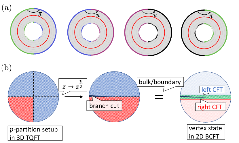
We have to mention that the -vertex state is defined after the conformal map (see Fig. 5),
| (26) |
The reason is as follows. On the one hand, the multipartite entanglement measures are computed on the two-dimensional spatial sphere with a -partition setup. On the other hand, by definition, the density matrix of -vertex state is defined on the spacetime manifold with four excess angles, each takes the value as shown in Fig. 5 (a) (and after taking the trace of , the spacetime path integral becomes a genus). Thus, the conformal transformation in Eq. (26) is required to bridge them, as shown in Fig. 5 (b). If this is not included, the final results for all entanglement measures would carry an extra factor of .
III.2 Entanglement entropy with corner contribution
We are now ready to calculate the entanglement entropies , , and associated to the regions , , and . in Fig. 4(b). The multipartition can be done by using the -vertex state. The corresponding replica path integral for computing -th Rényi entropy is defined on a Riemann surface. For example, when , the path integral is on a Riemann surface with genus . The path integral on the higher genus surface is not readily obtained. However, in the limit of , it can be evaluated by using the path integral decomposition described in Sec. II.3. Here, we factorize the partition function (with closed boundary condition) into two with open boundary condition by inserting a complete set of states. In the limit , the open partition function can be approximated by taking the leading twisted operator or vacuum. Thus, the replica partition function can be approximated by . The constant is a combination of the normalization factor and the coefficient , which contributes to the entanglement entropy as the topological entropy, as discussed in Eq. (20). This strip partition function can be illustrated as in Fig. 6 for the case of , where the width and length of each strip are and , respectively. We take two intervals and as shown in the figure, namely, the two bulk regions are adjacent. The intervals and denote the -th fold branch cut when evaluating -th Rényi entropy.
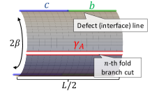
The entanglement entropy and can be computed by the open partition function . To evaluate the partition function , we consider the following conformal maps (the following figures are illustrated for ):
-
(i)
Mapping from cylinder to hemisphere: .
-
(ii)
Rotating : .
(insertion points of twist operators mapped to )
-
(iii)
Unwrapping: and gluing copies.
![[Uncaptioned image]](/html/2301.07130/assets/x10.png)
-
(iv)
Rotating : .
(insertion points of twist operators mapped to )
-
(v)
Mapping from sphere to cylinder .
![[Uncaptioned image]](/html/2301.07130/assets/x11.png)
In Step (iv), the interval is mapped to and the interval is mapped to . The cutoff at the end of the intervals () transforms as
| (27) | ||||
The interval is mapped to . By using Eq. (22) with the modified cutoffs in Eq. (27) (), and the normalization factor from Eq. (16) and the coefficient from Eq. (17), the entanglement entropy including the corner contribution is given by
| (28) | ||||
The topological term comes from the anyons insertion and , where unique fusion channel is assumed (as commented in the last paragraph of Sec. II.1). We set as the trivial interface from now on. In this expression the factor is removed by Eq. (26). Similarly, to find the entanglement entropy for interval , we can perform an additional shift such that the interval is mapped to and apply Eq. (23):
| (29) | ||||
And similarly, for ,
| (30) |
Combining these results, we can also obtain the mutual information:
| (31) | ||||
The above results, presented for , can be readily generalized to . I.e., subregion has a cusp with angle . The entanglement entropy in this case is given by
| (32) |
This is the central result of this section. The second term can be identified as the corner contribution to the entanglement entropy. Recalling that we have two corners with equal angles in our setup, we may introduce that represents contribution from each corner (with the minus sign to be consistent with the convention in [12, 13, 14]. We note that takes the same form as the entanglement entropy of the ground state of (1+1)d CFT on a finite periodic chain (of length ) associated with an interval (of length ). It is known that the same contribution arises when the subregion of our interest includes a physical edge [17], although there is no physical edge in our setup.
In Sec. V, we will compute the corner contribution for the case of the free Majorana fermion CFT () and . There, we will construct the vertex states explicitly, and calculate the bipartite entanglement entropy numerically. We will confirm, within numerical errors, the above result (32).
We also note that the corner contribution was previously discussed in the literature for the integer quantum Hall ground states [12, 13, 14]. In [13], it was numerically observed that the corner contribution (from one corner) behaves as for small while for , where numerical constants and were determined numerically. While the latter behavior of the corner contribution near is consistent with ours, the small behavior disagrees with . We also note that in [13], the constant is estimated for the integer quantum Hall state as , that should be contrasted with with for . The source of the discrepancy is not entirely clear. We nevertheless recall that the (single-particle) bipartite entanglement spectrum for the integer quantum Hall state in the lowest Landau level is linear only for small momentum along the entangling boundary [32], while in our ansatz state (5) a perfectly relativistic spectrum is assumed. It is also possible that for small enough , the representation of the topological ground state near the cusp by using the vertex state, , is not entirely accurate. Our numerics in Sec. V, where we verify the formula (32) for relatively large by using the explicit form of , is in favor of these speculations. Finally, we should also note that not all bulk geometrical properties of topological liquid may be captured by using the edge states and the bulk-boundary correspondence [33].
IV Reflected entropy and Markov gap
In this section, we consider the multipartition setup as in Fig. 4(b) and compute the reflected entropy as well as the Markov gap for the -vertex state for the case where and are adjacent and . We will show that the Markov gap is analytically.
Let us first define the reflected entropy and its replica path integral. The reflected entropy is a correlation measure that captures the tripartite entanglement. Given a reduced density matrix supported on , one can obtain its canonical purification state which is supported on , and , are identical copies of (up to complex conjugation). The reflected entropy is defined as the von Neumann entanglement entropy of the state after tracing out :
| (33) |
In the following, we will use the replica trick to compute the reflected entropy.
To compute the reflected entropy, two replica indices shall be introduced and the open partition function to be evaluated is:
| (34) |
Here is the index for Rényi replicas, and is the index for handling the square root of the reduced density matrix, where we take at the end of the calculation. The -th Rényi reflected entropy is computed using:
| (35) |
and the reflected entropy is .
Similar to the previous discussion, the path integral for evaluating is performed on a higher genus surface and is hard to compute. Using the path-integral decomposition as in Sec. II.3, we again focus on the open partition function. For reflected entropy, the normalization factor and the density of the lowest energy states become highly complicated. Therefore, we first focus on the special case where the topological term can be neglected and give a few comments later.
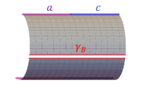
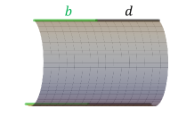
To evaluate the partition function , we consider the following conformal maps. The steps (i)-(iv) are the same as in Sec. III.2, and the conformal maps from step (v) are:
-
(v)
Unwrapping: .
![[Uncaptioned image]](/html/2301.07130/assets/x12.png)
-
(vi)
Rotating : .
(insertion points of twist operators mapped to )
-
(vii)
Unwrapping: .
-
(viii)
Map from sphere to cylinder: .
![[Uncaptioned image]](/html/2301.07130/assets/x13.png)
After the above conformal transformations, is brought to a partition function on a cylinder with interfaces, and with a new cutoff:
| (36) |
This conformal factor is the OPE coefficient of twist operators [7]. Since we assume the interfaces to be topological, we can freely move junction fields so that the net of the interfaces is simplified as shown in step (viii), where .
Using the new cutoff , the reflected entropy can be evaluated by Eq. (22):
| (37) | ||||
where we use the assumption that the topological contribution is zero. Taking into account the effect of the conformal map (26), we obtain the reflected entropy for the -partition setup,
| (38) |
The first term corresponds to the area law term. The second term comes from the conformal transformation (27). This term can be understood as a corner contribution. The third term comes from the factor in (36). This is the universal contribution related to the OPE coefficient .
With the above results on mutual information and reflected entropy, let us now evaluate the Markov gap. Combining the results from the previous two subsections and assuming the topological contribution can be neglected, we find the Markov gap is:
| (39) |
In summary, the corner contribution from mutual information and reflected entropy cancel out exactly, and the Markov gap does not receive the corner contribution. This is verified numerically in the Majorana fermion CFT in Sec. V.
Now, to reiterate, we restricted our computation to the case in which the reflected entropy does not receive additional topological contributions from anyon insertions. In previous sections, we considered configurations in which a single pair of anyons pierces each interface, with the anyon label being determined by the corresponding interface operator, as depicted in Fig. 4(b). While we have been unable to compute the Markov gap in this more general case, we suspect that it should still vanish. Indeed, as noted in the Introduction, Ref. [9] proved that the Markov gap vanishes for so-called “sum-of-triangle” states. For a tripartition of a Hilbert space and further bipartitions of each subspace, a sum of triangle states takes the form
where and has support in . Qualitatively, the anyon configuration Fig. 4(b) takes this triangle state form, with each anyon pair entangling two of the three subregions. Based on this heuristic, we suspect that this particular configuration of anyons will not lead to a non-zero Markov gap. It is possible that other, non-trivial anyon configurations could lead to a non-vanishing Markov gap.
V Four-vertex states in the Majorana fermion CFT and correlation measures
In this section, we consider the free real fermion CFT with , and construct four-vertex states explicitly. From the explicit form of the vertex states, various correlations measures (entanglement entropy, reflected entropy, entanglement negativity, etc.) can be calculated numerically. We will see that the numerics is consistent with the analytical results in the preceding sections. In addition, we can calculate the correlation measures in the setups that are not amendable in the analytical treatment. For example, we will discuss the correlation measures when subregions and are not adjacent.
In the following, we will present two approaches to construct vertex states; the direct method and the Neumann function method [34, 35, 36, 37, 3]. We will also note that there are at least two vertex states, which satisfy what we call “usual” and “kink” boundary conditions. We will show that the Neumann function method, when applied naively, gives rise to the vertex state with the kink boundary condition, and the kink boundary condition reproduces the correlation measures as predicted in the previous sections.
V.1 Usual and kink boundary conditions
Let us consider four copies of the Majorana fermion CFT and construct the vertex state. We denote the Majorana fermion fields by where denotes the copy index, and coordinatizes the spatial circle. For simplicity in this section we set the circumference of the circle to be . They satisfy the canonical anticommutation relation . We will work with the Neveu-Schwartz (antiperiodic) boundary condition in . Under the antiperiodic boundary condition, the fermion field can be expended in the Fourier modes labeled by half-integers as . Using the Fourier modes, the canonical anticommutation relation reads .
As discussed in Sec. III.1, we define a vertex state in terms of the boundary condition it satisfies. First, we introduce the usual boundary condition by
| (40) |
where , and the periodic boundary condition is understood. On the other hand, we introduce the kink boundary condition by
| (41) | ||||
where again . Here, we observe that the boundary state – which can be regarded as the two-vertex state – satisfies a similar kink boundary condition: (). The kink boundary condition is “natural” from this perspective. We will also see that the Neumann function method applied -vertex states with even naturally gives rise to the kind boundary condition. We will see below that the kink boundary condition yields the predicted entanglement behaviors in Secs. III and IV.
V.2 Direct method
We first present the Dirac method, which is able to solve for the vertex state for both usual and kink boundary conditions. Since there is no interaction, the solution to Eq. (40) or (41) can be explicitly constructed as a coherent state (Gaussian state). For simplicity, we will focus below the usual boundary condition and delegate the details for the case of the kink boundary condition to Appendix C. It can be numerically verified that for the kink boundary, direct calculation method gives the same result as the Neumann coefficient method.
The boundary condition (40) can be diagonalized by a unitary transformation. Explicitly, we introduce the “rotated” fields as where the unitary matrix is given by
| (46) |
The transformed fields obey the anticommutation relation . We note that the matrix diagonalizes the “shift” matrix as
| (47) |
The original boundary condition is translated into the boundary condition of the transformed fields :
| (48) | ||||
We note that the boundary conditions for and are decoupled and take the form () where or . The solution to this boundary condition is derived in [3] and given by
| (49) |
where is the ground state of the -fermion field. Given , the explicit form of is summarized in Appendix B. As for the boundary conditions for and , they can be written in terms of the Fourier modes as
| (50) |
The modes with different decouple, which allows a simple boundary state solution.
To summarize, the vertex state in the basis can be constructed as where the matrix is given by
| (51) |
in the basis . Finally, can be written in the original basis by “rotating back”,
| (52) |
where the matrix is obtained from as .
V.3 Neumann function method
In the Neumann function method, we start from the Gaussian ansatz solution of the form (52) and find the matrix such that the vertex state reproduces the two-point correlation function (Neumann function) on the plane. (The latter condition can be thought of as the definition of vertex states – see Ref. [3].) Specifically, we consider the two-point correlation function of the fermion field on the complex plane and consider
| (53) |
Here, is the conformal transformation from copies of half cylinders to the full complex plane:
| (54) |
with the constant term satisfies . From the Fourier transform of the Neumann function we read off as
| (55) |
From the given Neumann function (53) one can check explicitly the presence of the second term (“singular term”) – see Appendix D for details.
In order to see the boundary condition satisfied by the so-constructed vertex state, we need to check the behavior of the Neumann function under the reflection . This amounts to and leads to:
| (56) | ||||
On the other hand, the derivative is transformed as
| (57) |
where we noted
| (58) |
To satisfy the usual boundary condition (), we need to choose to branch cut of such that:
| (59) |
For , this leads to , which cannot be satisfied no matter how the branch cut is chosen. On the other hand, the kink boundary condition is
| (60) | ||||
which can be satisfied by choosing and .
To summarize, from the Neumann function (53), we can construct the vertex state obeying the kink boundary condition explicitly as a fermionic Gaussian state with the coefficient in (55). More details and the explicit form of the matrix are given in Appendix D.
| Partition | 1 | 2 | 3 | |
![[Uncaptioned image]](/html/2301.07130/assets/x14.png) |
![[Uncaptioned image]](/html/2301.07130/assets/x15.png) |
![[Uncaptioned image]](/html/2301.07130/assets/x16.png) |
||
| (p) | 41.2389 | 41.1811 | 82.2467 | |
| (k) | 41.2389 | 41.1811 | 82.2467 | |
| (u) | 41.2389 | 41.1811 | 82.2467 | |
| (p) | 41.1234 | 41.2389 | 0.1155 | |
| (k) | 41.1233 | 41.2389 | 0.1155 | |
| (u) | 41.1233 | 41.2389 | 0.1155 | |
| (p) | 41.2389 | 41.3544 | 0.2471 | |
| (k) | 41.2389 | 41.3544 | 0.2471 | |
| (u) | 41.2276 | 41.3481 | 0.2471 | |
| (p) | 0.1316 | |||
| (k) | 0.1155 | 0.1155 | 0.1316 | |
| (u) | 0.1043 | 0.1093 | 0.1316 | |
| (p) | 30.8425 | 30.9292 | - | |
| (k) | 30.8185 | 30.9054 | 0.0708 | |
| (u) | 30.8191 | 30.9054 | 0.0708 | |
V.4 Correlation measures
With the explicit forms of the vertex states and , we are ready to calculate the correlation measures, i.e., entanglement entropy, mutual information, reflected entropy, and entanglement negativity. As the constructed vertex states are Gaussian, we can calculate these quantities numerically and efficiently [38, 39, 40, 41]. Specifically, we partition the 4 copies of the CFTs (edge states) into three parties, , , and the compliment of . The particular partitions we consider are listed in Table 1. The first two partitions correspond to the case where subregions and are adjacent which can be directly compared with the analytical results in the previous sections, as we will discuss in details below. We set the regulator (cutoff) in this subsection. We also recall that the circumference is set to .
First, for the entanglement entropy of bipartition , the two boundary conditions give the same result. For Partitions 1 and 2, we can also check that the numerics agrees with the prediction Eq. (32). Here, we note that we need to restore the extra contribution discussed in Eq. (26) and that the topological piece is zero, , in the free fermion model,
| (61) |
where for Partition 1 and 2, respectively.
For Partition 3 where the region consists of two disconnected parts ( and ), the calculation in Sec. III does not apply since the subregion was assumed to be simply connected there. Nevertheless, recall that we observed below Eq. (32) the corner contribution is identical to the bipartite entanglement entropy of the ground state of (1+1)-dimensional CFT. Motivated by this, it is then tempting to compare the numerical result for Partition 3 with the entanglement entropy of the ground state of (1+1)-dimensional CFT with disjoint intervals. For the free fermion CFT, it is given by [42]
| (62) | ||||
where the end points of the two disjoint intervals and using the cord coordinate are given by , and . Thus, we compare our numerics with
| (63) |
Here, the factor of 2 in the first term comes from doubling the number of twist operators in this case. The mutual information can be obtained from . As demonstrated in Table 1, the numerics agrees well with Eq. (63).
Unlike the entanglement entropy and mutual information , we found that the reflected entropy and Markov gap depend on the boundary conditions. For Partitions 1 and 2, we checked that the numerical results with the kind boundary condition agree with the CFT prediction (38), and reproduce the Markov gap . For Partition 3, the usual and kink boundary conditions seem to give the same result. Once again, the CFT prediction (38) is not directly applicable here since region and are not adjacent. Nevertheless, the numerical calculation on the 1d free fermion model shows (when extrapolating to ), which again agrees with the above prediction.
We can also discuss logarithmic negativity for the same configurations 1,2 and 3. For the case of integer quantum Hall states, logarithmic negativity in these configurations was studied in Ref. [19]. While we do not have the corresponding CFT calculations along the line of Sec. III and Sec. IV, we once again borrow the corresponding one-dimensional result [43], leading to the following prediction:
| (64) |
when region and are adjacent. For Partition 2, the predicted value is , which does not match perfectly with 30.8185 from numerics. Nevertheless, the difference between the negativities for Partition 1 and 2 is , and close to the predicted value .
There is a potential ambiguity in the term in the one-dimensional result for logarithmic negativity due to the OPE coefficient between twist operators. Unlike the reflected entropy, where the OPE coefficient is universal, depending only on the central charge, the OPE for negativity depends on the full operator content of the theory because the replica manifold is a Riemann surface with genus growing with replica number (see Appendix E for details). We have set the OPE coefficient to one by hand and have found good agreement with numerics.
VI Discussion
In this work, we developed an analytical approach to calculate the corner contribution to bipartite entanglement entropy and multipartite entanglement quantities (reflected entropy and Markov gap in particular) for generic (2+1)-dimensional topologically-ordered ground states. Some of our central results are presented in Eqs. (32), (38) and (39). This then supports the conjecture on the Markov gap made in the previous works by looking at examples, . We hope this analytical approach helps us better understand the conjecture that relates the Markov gap and gappable boundaries. It is of fundamental importance to understand this better.
An important future work is to compute purely from the bulk-perspective, using TQFT. This was done for many entanglement quantities in various configurations by using surgery method in TQFT. If this were possible, the entanglement quantity would be written in terms of the data of the TQFT. However, TQFT knows the central charge only mod 8 (by the Gauss-Milgram formula). One would then speculate that it would then be necessary to have, perhaps, fully-extended TQFT.
At a technical level, another challenge is to understand the contribution from the topological interface in the reflected entropy calculation in the general cases. In the above calculation, we focus on the Ishibashi vacuum interface which corresponds to the d ground state of topological order on the sphere. For higher genus systems, the anyon insertions in the non-contractible loops will lead to degenerate ground states , where in general . Whether would receive topological contribution in this general case is an open question. It would be also desirable to extend our calculations to incorporate the presence of non-Abelian anyons.
Acknowledgement
This work is supported by the National Science Foundation under Award No. DMR-2001181, a Simons Investigator Grant fromthe Simons Foundation (Award No. 566116), and the Gordon and Betty Moore Foundation through Grant GBMF8685 toward the Princeton theory program. This work was performed in part at Aspen Center for Physics, which is supported by National Science Foundation grant PHY-1607611. YL was supported in part by the National Science Foundation under Grant No. NSF PHY-1748958, the Heising-Simons Foundation, and the Simons Foundation (216179, LB) at the Kavli Institute for Theoretical Physics. JKF is supported by the Institute for Advanced Study and the National Science Foundation under Grant No. PHY-2207584. YK is supported by the Brinson Prize Fellowship at Caltech and the U.S. Department of Energy, Office of Science, Office of High Energy Physics, under Award Number DE-SC0011632.
Appendix A Reflected entropy for pure state
In this appendix we use conformal interface approach to reproduce a well-known result: If is a density matrix for a pure state, then . This serves as another consistency check for the validity of the conformal interface method.
Recall that Rényi reflected entropy is computed using the replica trick:
| (65) |
where was defined in Eq. (34). Here, is the Rényi replica index, and is the replica index for handling square root of the density matrix. In left hand side of Fig. 7(a), we take as an example and draw the path integral representation for each Rényi replica in . The black dashed lines indicates the gluing within the same Rényi replica, while the cuts with blue and orange annotations are glued to the next (or previous) Rényi replica. After taking Rényi replicas, we obtain two cylinder path integral with circumference , and cylinder path integral with circumference . Note all the cylinders have length and periodic boundary condition is taken implicitly (which makes them torus).
Similarly, the path integral representation for will yield cylinder path integral with circumference . Combining the result of and , we find is equal to the square of from the calculation, as shown in Fig. 7(b). After taking the logarithmic, we come to the conclusion that , thus after taking the Rényi replica limit .
Appendix B Solution to single fermion boundary condition
In this section, we give the solution of a single fermion boundary condition, which is useful in the direct method for obtaining the vertex state. Here, the solution is stated without proof and we refer to [3] for the detailed derivation.
The single fermion boundary condition is formulated as:
| (66) |
with the consistency relation . To write down the solution, let’s first expand in terms of the Fourier modes: . If we define matrix with components , the boundary condition in terms of the Fourier mode is , where runs through both positive and negative half integers. To separate the creation operators ( with negative ) and annihilation operators ( with positive ), we then introduce a block structure:
| (67) | ||||
In the above blocks only take positive values, namely, . We state without proof that the solution of boundary condition (66) is:
| (68) |
where matrix is given in terms of the four blocks of matrix:
| (69) |
In the discussion of the vertex state, the function takes the form of , which carries a parameter . The corresponding matrices and are denoted as and .
Appendix C Direction method: kink boundary condition
In this appendix, we solve the vertex state with kink boundary condition by the direct method. As a consistency check, we have numerically verified that this solution is the same as obtained from the Neumann coefficient method.
Consider the kink boundary condition on ,
| (70) | ||||
We would like to find a matrix that diagonalizes the “shift” matrix and use it to rotate the basis. The boundary condition thus decouples in the rotated basis. To start, we notice the “shift” matrix can be diagonalized by:
| (71) |
with unitary matrix :
| (72) |
The rotated real fermions are thus . By
| (73) |
the anticommutation relation of the rotated basis is .
Let’s first consider the pair. For , the boundary condition is:
| (74) | ||||
This amounts to choosing in the boundary condition (). Similarly, for , the corresponding angle is . Now in terms of the Fourier modes, the boundary condition can be rewritten as:
| (75) |
We can separate the creation and annihilation parts explicitly, where :
| (76) |
from which we read out:
| (77) | ||||
Using the four block matrices, the vertex state solution for pair is:
| (78) | ||||
Similarly, for the pair, the corresponding angles are and , and can be obtained in a similar way. Finally, we need to rotate back to the original basis. The vertex state solution in the basis is thus:
| (79) | ||||
Although the vertex state solution for kink boundary condition can be obtained from either the direct method or the Neumann coefficient method, the Neumann coefficient method is more desirable for numerical calculation, because it does not involve the matrix inverse which would lead to numerical inaccuracy.
Appendix D Neumann coefficient method: Explicit form of solution
In this appendix, we write down the explicit form of vertex state solution with kink boundary condition by finding the mode expansion of in Eq. (53):
| (80) |
Here is the conformal transformation that brings copies of half cylinders to a complex plane:
| (81) |
with the constant terms satisfy . In the following we aim to write in terms of mode expansion :
| (82) |
To do so, we will write down the mode expansion of and .
Let us start from the mode expansion of . Using:
| (83) |
and we denote
| (84) |
the factor can be rewritten as:
| (85) |
We thus need to obtain the mode expansion of .
For , the coefficients satisfy the recursion relation:
| (86) |
and the first two coefficients are . This with the recursion relation allows us to obtain all the .
Next, we would need to rewrite . By using we can obtain:
| (87) | ||||
For the four-vertex state, take values from . Since only depends on the difference between and , there are four difference circumstances. For :
| (89) |
For :
| (90) |
For :
| (91) |
For :
| (92) |
To evaluate the expansion coefficients of , we need to use the following two relations:
| (93) | ||||
where denotes the singular term ; and
| (94) | ||||
The above two relations can be derived using:
and
By plugging (93) and (94) into (89) - (92), we obtain the mode expansion coefficients of . We summarize the explicit expressions below.
D.1 Summary
To summarize, the mode expansions for are:
| (95) | ||||
One nice feature is that the singular terms in take the form:
| (96) |
which is what we desired in order to satisfy the boundary condition (as discussed near Eq. (55)).
Let’s denote , , and . The whole matrix is:
| (97) |
As a consistency check, let us verify is antisymmetric. Note that by definition is antisymmetric and is symmetric. Using our previous choice of branch cut ( and ), the factors are , , so the blocks associated with has the desired property under tranposition. For the blocks associated with and , for example:
| (98) |
Using our previous choice, . One can check:
which shows this block is indeed antisymmetric. Note that the antisymmetric property is dependent on the choice of . If we make another choice of branch cut , this block would not be antisymmetric.
Appendix E One-dimensional CFT
In 1+1D CFT, one may use the twist operator formalism to compute various quantum information inequalities. In this appendix, we review how to evaluate the mutual information, reflected entropy, and logarithmic negativity for adjacent intervals in the vacuum.
The moments of the reduced density matrix are given by the two-point function of twist operators located at the entangling surfaces [42]
| (99) |
which is fixed by conformal symmetry
| (100) |
Taking the replica limit, we find
| (101) |
Because the union of adjacent intervals is again an interval, we immediately find
| (102) |
The reflected entropy for adjacent intervals may also be computed using the twist operator formalism as a three-point function [7]
| (103) |
This is also completely fixed by conformal symmetry, up to a nontrivial OPE coefficient
| (104) |
The evaluation of this OPE coefficient is crucial because it is precisely what leads to a nontrivial Markov gap. It is useful to consult the Riemann-Hurwitz formula to compute the genus of the replica manifold
| (105) |
where is the total number of replicas and is the number of sheets that meet at the branch point. From the definition of the twist fields, one concludes that the genus for all and is zero, so the OPE coefficient is universal, only dependent on the central charge of the theory. Explicitly, it is given by [7]
| (106) |
which precisely leads to the universal Markov gap.
We proceed to the negativity, which is computed by a different three-point correlation function of twist operators [43]
| (107) |
where the middle twist operator applies a double cyclic permutation. The limit is taken from the even integers to one. Of course, this is still fixed by conformal symmetry, up to the OPE coefficient
| (108) |
with the same scaling as mutual information and reflected entropy. A significant different arises however when considering the OPE coefficient. The replica manifold for even can be seen to have genus . Partitiln functions on non-zero genus surfaces depend on the full operator content of the theory so the OPE coefficient is nonuniversal. We therefore cannot expect a simple analytic function in analogous to the reflected entropy. In the main text, we have set by hand, finding good agreement with numerics.
References
- Kitaev and Preskill [2006] A. Kitaev and J. Preskill, Topological Entanglement Entropy, Phys. Rev. Lett. 96, 110404 (2006), arXiv:hep-th/0510092 [hep-th] .
- Levin and Wen [2006] M. Levin and X.-G. Wen, Detecting Topological Order in a Ground State Wave Function, Phys. Rev. Lett. 96, 110405 (2006), arXiv:cond-mat/0510613 [cond-mat.str-el] .
- Liu et al. [2022] Y. Liu, R. Sohal, J. Kudler-Flam, and S. Ryu, Multipartitioning topological phases by vertex states and quantum entanglement, Phys. Rev. B 105, 115107 (2022), arXiv:2110.11980 [cond-mat.str-el] .
- Siva et al. [2022] K. Siva, Y. Zou, T. Soejima, R. S. K. Mong, and M. P. Zaletel, Universal tripartite entanglement signature of ungappable edge states, Phys. Rev. B 106, L041107 (2022).
- Kim et al. [2022a] I. H. Kim, B. Shi, K. Kato, and V. V. Albert, Chiral Central Charge from a Single Bulk Wave Function, Phys. Rev. Lett. 128, 176402 (2022a), arXiv:2110.06932 [quant-ph] .
- Kim et al. [2022b] I. H. Kim, B. Shi, K. Kato, and V. V. Albert, Modular commutator in gapped quantum many-body systems, Phys. Rev. B 106, 075147 (2022b), arXiv:2110.10400 [quant-ph] .
- Dutta and Faulkner [2021] S. Dutta and T. Faulkner, A canonical purification for the entanglement wedge cross-section, Journal of High Energy Physics 2021, 178 (2021).
- Akers and Rath [2020] C. Akers and P. Rath, Entanglement wedge cross sections require tripartite entanglement, Journal of High Energy Physics 2020, 10.1007/jhep04(2020)208 (2020).
- Zou et al. [2021] Y. Zou, K. Siva, T. Soejima, R. S. K. Mong, and M. P. Zaletel, Universal Tripartite Entanglement in One-Dimensional Many-Body Systems, Phys. Rev. Lett. 126, 120501 (2021), arXiv:2011.11864 [quant-ph] .
- Note [1] See Ref. [44] for further discussion that gave the Markov gap its name.
- [11] R. Sohal, and S. Ryu (in preparation).
- Rodríguez and Sierra [2010] I. D. Rodríguez and G. Sierra, Entanglement entropy of integer quantum hall states in polygonal domains, Journal of Statistical Mechanics: Theory and Experiment 2010, P12033 (2010).
- Sirois et al. [2021] B. Sirois, L. M. Fournier, J. Leduc, and W. Witczak-Krempa, Geometric entanglement in integer quantum Hall states, Phys. Rev. B 103, 115115 (2021).
- Ye et al. [2022a] D. Ye, Y. Yang, Q. Li, and Z.-X. Hu, Entanglement entropy of the quantum hall edge and its geometric contribution, Frontiers in Physics 10, 10.3389/fphy.2022.971423 (2022a).
- Estienne et al. [2022] B. Estienne, J.-M. Stéphan, and W. Witczak-Krempa, Cornering the universal shape of fluctuations, Nature Communications 13, 10.1038/s41467-021-27727-1 (2022).
- Berthiere et al. [2022] C. Berthiere, B. Estienne, J.-M. Stéphan, and W. Witczak-Krempa, Full-counting statistics of charge fluctuations in quantum hall states (2022).
- Estienne and Stéphan [2020] B. Estienne and J.-M. Stéphan, Entanglement spectroscopy of chiral edge modes in the quantum hall effect, Physical Review B 101, 10.1103/physrevb.101.115136 (2020).
- Ye et al. [2022b] D. Ye, Y. Yang, Q. Li, and Z.-X. Hu, Entanglement entropy of the quantum hall edge and its geometric contribution, Frontiers in Physics 10, 10.3389/fphy.2022.971423 (2022b).
- Liu et al. [2022] C.-C. Liu, J. Geoffrion, and W. Witczak-Krempa, Entanglement negativity versus mutual information in the quantum hall effect and beyond (2022).
- Avron et al. [1992] J. E. Avron, M. Klein, A. Pnueli, and L. Sadun, Hall conductance and adiabatic charge transport of leaky tori, Phys. Rev. Lett. 69, 128 (1992).
- Can [2017] T. Can, Central charge from adiabatic transport of cusp singularities in the quantum hall effect, Journal of Physics A: Mathematical and Theoretical 50, 174004 (2017).
- Can and Wiegmann [2017] T. Can and P. Wiegmann, Quantum Hall states and conformal field theory on a singular surface, Journal of Physics A Mathematical General 50, 494003 (2017), arXiv:1709.04397 [hep-th] .
- Ishibashi [1989] N. Ishibashi, The Boundary and Crosscap States in Conformal Field Theories, Mod. Phys. Lett. A 4, 251 (1989).
- Qi et al. [2012] X.-L. Qi, H. Katsura, and A. W. W. Ludwig, General relationship between the entanglement spectrum and the edge state spectrum of topological quantum states, Phys. Rev. Lett. 108, 196402 (2012).
- Wen et al. [2016] X. Wen, S. Matsuura, and S. Ryu, Edge theory approach to topological entanglement entropy, mutual information, and entanglement negativity in Chern-Simons theories, Phys. Rev. B 93, 245140 (2016), arXiv:1603.08534 [cond-mat.mes-hall] .
- Cardy [2004] J. Cardy, Boundary conformal field theory 10.48550/ARXIV.HEP-TH/0411189 (2004).
- Sakai and Satoh [2008] K. Sakai and Y. Satoh, Entanglement through conformal interfaces, Journal of High Energy Physics 2008, 001 (2008), arXiv:0809.4548 [hep-th] .
- Brehm et al. [2016] E. Brehm, I. Brunner, D. Jaud, and C. Schmidt-Colinet, Entanglement and topological interfaces, Fortschritte der Physik 64, 516 (2016), arXiv:1512.05945 [hep-th] .
- Note [2] We treat our BCFT as an interface CFT (ICFT) by the unfolding. Then, the ICFT corresponds to a chiral part of the BCFT.
- Note [3] While the first line appears to indicate that we have a single path-integral representation for , due to the normalization of the Ishibashi states, we need separate path integrals for the numerators and denominators. If we were to interpret as a single path integral, the normalization factors would contribute to the spectrum as states with negative dimension. This subtlety, however, does not matter in the limit where we only keep the vacuum block as in the last line.
- Kusuki [2022] Y. Kusuki, Reflected Entropy in Boundary/Interface Conformal Field Theory, arXiv e-prints , arXiv:2206.04630 (2022), arXiv:2206.04630 [hep-th] .
- Rodríguez and Sierra [2009] I. D. Rodríguez and G. Sierra, Entanglement entropy of integer quantum hall states, Physical Review B 80, 10.1103/physrevb.80.153303 (2009).
- Gromov et al. [2016] A. Gromov, K. Jensen, and A. G. Abanov, Boundary effective action for quantum hall states, Physical Review Letters 116, 10.1103/physrevlett.116.126802 (2016).
- Gross and Jevicki [1987] D. J. Gross and A. Jevicki, Operator formulation of interacting string field theory (III). NSR superstring, Nuclear Physics B 293, 29 (1987).
- Leclair et al. [1989] A. Leclair, M. E. Peskin, and C. R. Preitschopf, String field theory on the conformal plane (I).. Kinematical Principles, Nuclear Physics B 317, 411 (1989).
- Imamura et al. [2006] Y. Imamura, H. Isono, and Y. Matsuo, Boundary States in the Open String Channel and CFT near a Corner, Progress of Theoretical Physics 115, 979 (2006), arXiv:hep-th/0512098 [hep-th] .
- Imamura et al. [2008] Y. Imamura, H. Isono, and Y. Matsuo, Boundary State of Superstring in Open String Channel, Progress of Theoretical Physics 119, 643 (2008).
- Peschel [2003] I. Peschel, Calculation of reduced density matrices from correlation functions, Journal of Physics A: Mathematical and General 36, L205 (2003).
- Bueno and Casini [2020] P. Bueno and H. Casini, Reflected entropy for free scalars, Journal of High Energy Physics 2020, 10.1007/jhep11(2020)148 (2020).
- Shapourian et al. [2017] H. Shapourian, K. Shiozaki, and S. Ryu, Partial time-reversal transformation and entanglement negativity in fermionic systems, Physical Review B 95, 10.1103/physrevb.95.165101 (2017).
- Shapourian and Ryu [2019] H. Shapourian and S. Ryu, Entanglement negativity of fermions: Monotonicity, separability criterion, and classification of few-mode states, Physical Review A 99, 10.1103/physreva.99.022310 (2019).
- Calabrese and Cardy [2009] P. Calabrese and J. Cardy, Entanglement entropy and conformal field theory, Journal of Physics A Mathematical General 42, 504005 (2009), arXiv:0905.4013 [cond-mat.stat-mech] .
- Calabrese et al. [2012] P. Calabrese, J. Cardy, and E. Tonni, Entanglement negativity in quantum field theory, Physical Review Letters 109, 10.1103/physrevlett.109.130502 (2012).
- Hayden et al. [2021] P. Hayden, O. Parrikar, and J. Sorce, The Markov gap for geometric reflected entropy, Journal of High Energy Physics 2021, 47 (2021), arXiv:2107.00009 [hep-th] .