Eddington accreting Black Holes in the Epoch of Reionization.

Abstract

The evolution of the luminosity function (LF) of Active Galactic Nuclei (AGNs) at $z\lower 2.15277pt\hbox{$\;\buildrel>\over{\sim}\;$}5$ represents a key constraint to understand their contribution to the ionizing photon budget necessary to trigger the last phase transition in the Universe, i.e. the epoch of Reionization. Recent searches for bright high-z AGNs suggest that the space densities of this population at $z>4$ has to be revised upwards, and sparks new questions about their evolutionary paths. Gas accretion is the key physical mechanism to understand both the distribution of luminous sources and the growth of central Super-Massive Black Holes (SMBHs). In this work, we model the high-z AGN-LF assuming that high-z luminous AGN shine at their Eddington limit: we derive the expected evolution as a function of the “duty-cycle” ($f_{\rm dc}$), i.e. the fraction of life-time that a given SMBH spends accreting at the Eddington rate. Our results show that intermediate values ($f_{\rm dc}\simeq 0.1$) predict the best agreement with the ionizing background and photoionization rate, but do not provide enough ionizing photons to account for the observed evolution of the hydrogen neutral fraction. Smaller values ($f_{\rm dc}\lower 2.15277pt\hbox{$\;\buildrel<\over{\sim}\;$}0.05$) are required for AGNs to be the dominant population responsible for Hydrogen reionization in the Early Universe. We then show that this low-$f_{\rm dc}$ evolution can be reconciled with the current constraints on Helium reionization, although it implies a relatively large number of inactive SMBHs at $z\lower 2.15277pt\hbox{$\;\buildrel>\over{\sim}\;$}5$, in tension with SMBH growth models based on heavy seeding.

1 Introduction

The phase transition in the early Universe called Epoch of Reionization (EoR) marks an epoch of major transformation in baryonic properties, with the large majority of its hydrogen content moving from a neutral to an ionized state at $z\lower 2.15277pt\hbox{$\;\buildrel>\over{\sim}\;$}5.3$ (see e.g. Bosman et al., 2021, and references herein). EoR represents the epoch when the first complex astrophysical structures, i.e. galaxies, start to assemble, producing large amounts of stars in the process. As galaxies grow, Super-Massive Black Holes (SMBH) lying at their very centre also experience gas accretion, giving rise to the first Active Galactic Nuclei (AGN) and Quasar (QSO) phenomena. Both star formation and AGN activity are critical in the production of the ionizing photons required to drive the Universe outside the so-called Dark Ages.

Results from cosmological probes such as Planck (Planck Collaboration XVI, 2014) broadly constrain the redshift span of this transition to lie between $6<z<10$ with peak activity around $z\simeq 7$. The development of the EoR, its overall duration and topology have been the subject of major discussion in recent years, as these properties are directly linked to the astrophysical population responsible for the production of ionizing photons involved in the process. Generally speaking both Star Forming Galaxies (SFGs) and AGNs are likely contributors to the ionizing photon budget (Fontanot et al., 2012b), however their relative contribution is still matter of debate. This is not a secondary issue, as the nature of the dominant sources of ionizing photons are likely to affect the evolution of the process itself.

We expect that an EoR dominated by SFGs will start earlier and proceed for a relatively large redshift range ($6\lower 2.15277pt\hbox{$\;\buildrel<\over{\sim}\;$}z\lower 2.15277pt\hbox{$\;\buildrel<\over{\sim}\;$}15$) (see e.g. Bouwens et al., 2009): this is due to the fact that SFGs are numerous sources, but they produce a limited amount of ionizing photons per each $M_{\odot}/$yr of stellar mass formed. On the other hand, AGNs are a rare population, but they efficiently produce ionizing photons per each $M_{\odot}/$yr of gas accreted onto the SMBH (Telfer et al., 2002; Stevans et al., 2014): this implies that an AGNs-driven scenario favours a late and short EoR, that tends to be in better agreement with recent findings of a fast drop of both the mean free path of ionizing photons (Becker et al., 2021) and the space density of Ly_α emitters (Morales et al., 2021) at $z>6$.

The estimate of the redshift evolution of the space density of the AGN population (i.e. its luminosity function - LF - $\Phi$) at $z>5$ is thus of paramount relevance in order to estimate their relative contribution to the EoR. Such a goal is not an easy one as the robust derivation of completeness levels for different surveys is a complex task with controversial results, even for samples focusing only on the brightest-end of the LF (see e.g. Jiang et al., 2016; Yang et al., 2019, among the others): for example Schindler et al. (2019) show that the efficient selection of high-z QSOs in the SDSS does not correspond to high completeness levels. New efforts have recently allowed us to improve our understanding of this statistical estimator. The QUBRICS (QUasars as BRIght beacons for Cosmology in the Southern Hemisphere) survey (Calderone et al., 2019; Boutsia et al., 2020) is a prime example of a reliable QSOs candidate sample extracted from the combination of several observational databases (covering the wavelength range from the optical to the infrared) using machine learning techniques (Guarneri et al., 2021). Several of these candidates have been spectroscopically confirmed in the last few years (with a success rate close to 70 percent): the confirmed candidates have been then used to provide estimates for the bright-end of the AGN-LF at $z\simeq 3.9$ (Boutsia et al., 2021). Moreover, again using QUBRICS data, Grazian et al. (2022) estimate the space density for $M_{1450}\simeq-28.6$ AGNs at $4.5<z<5$, and find that it is consistent with a scenario of a pure density evolution between $z\simeq 3.9$ and $z\simeq 4.75$ with a parameter $\gamma=-0.25$. This $\gamma$ value is smaller (i.e. the evolution is slower) than the corresponding $\gamma=-0.38$ estimated from the ELQS (Extremely Luminous Quasar Survey, Schindler et al., 2019), and also from the extrapolation of lower-redshift results based on multi-wavelength surveys (Shen et al., 2020). The evolution of the AGN/QSO-LF represents a key aspect for models of the ionizing background, as it critically controls the total number of ionizing photons produced by accretion onto SMBHs events. Giallongo et al. (2015) first suggested (later confirmed in Giallongo et al. 2019) that a relatively high space density of faint AGNs may account for the total photon budget required for EoR (if these objects retain the same properties - e.g. spectral slope and escape fraction distribution - of their brighter counterparts). While finalising our study, preliminary results for AGN candidates in the JWST Cosmic Evolution Early Release Science Survey seem to strengthen the case for a high space density of faint AGNs at $z\simeq 5$ (Onoue et al., 2022). Moreover, comparing AGN-LFs with LFs for the total (inactive) galaxy population holds critical constraints for models of AGN feedback and their impact on galaxy evolution (see e.g. Fontanot et al., 2020, and reference herein).

While the search for reliable candidates and their spectroscopic confirmation is routinely performed by several groups both in the Northern and Southern skies, the finding of very bright QSOs at the edge of the EoR poses a number of theoretical challenges. Quasars like J031343.84-180636.4 (Wang et al., 2021, z=7.642), HSC J124353.93+010038.5 (Matsuoka et al., 2019, z=7.07), ULAS J134208.10+092838.61 (Bañados et al., 2018, z=7.54) or ULAS J112001.48+064124.3 (Mortlock et al., 2011, z=7.085) are all powered by SMBHs with estimated masses within 10⁸-10${}^{9}M_{\odot}$. The mere existence of such massive structures when the Universe is approximately 750 Myrs old is usually interpreted as an evidence for very efficient accretion onto SMBHs at early epochs (see e.g. Di Matteo et al., 2012).

Prompted by these considerations, in this work we will explore a simplified model based on the assumption that all SMBHs at $z>5$ (the redshift range where estimates for the AGN/QSO has been recently revised upwards) accrete at their Eddington limit for a fraction of their lifetime (i.e. the so-called “duty cycle”). We will then rescale this assumption into predictions for the evolution of the AGN/QSO-LF, and, consequently, on predictions for the contribution of the AGN population to the observed ionizing background. The overall exercise will give us hints on the number of ionizing photon associated with the early build-up of the more massive SMBHs that are available for EoR. Throughout the paper we assume a standard $\Lambda$ cold dark matter concordance cosmological model (i.e. $\Omega_{\Lambda}=0.7$, $\Omega_{m}=0.3$, $H_{0}=70\,{\rm km/s/Mpc}$) and we refer the absolute magnitude at 1450 Å ($M_{1450}$) to the AB system.

2 Modelling high-z SMBHs evolution

In order to estimate the redshift evolution of the QSO-LF we start from considering different scenarios for the growth of SMBH powering these luminous sources. For the purpose of the present work we have tried to adopt the simplest hypotheses allowing us to explore the general trends, well aware that some of the conclusions can be circumvented by more complex schemes. In particular, we assume that whenever a SMBH accretes material at $z\lower 2.15277pt\hbox{$\;\buildrel>\over{\sim}\;$}5$ it is doing so at the Eddington rate. We thus write its mass evolution using the following equation:

$$M_{\rm SMBH}(t)=M_{0}\,e^{\big{[}\frac{(1-\epsilon)}{\epsilon}\frac{f_{\rm dc}}{t_{\rm edd}}t\big{]}}$$ (1)

which includes three free parameters, namely the radiative efficiency $\epsilon$, the Eddington timescale $t_{\rm edd}=4.5\times 10^{8}$ yr and the fraction of time the SMBH is accreting $f_{\rm dc}$ (i.e. its “duty cycle”). Eq. 1 clearly shows that the growth at Eddington rate depends on both parameters $\epsilon$ and $f_{\rm dc}$. Nonetheless, in this study we prefer to fix $\epsilon=0.1$ as reference value, in order to maintain a physical understanding of our conclusions as a function of $f_{\rm dc}$. We briefly discuss the impact of a different choices for $\epsilon$ in the following sections: although the exact $f_{\rm dc}$ values quoted in the discussion may change, our conclusions are robust against reasonable combinations of parameters.

In this work, we will consider a backward approach: we start from observed AGN-LFs at the highest redshifts accessible with present-day surveys and we then try to assess the expected evolution to even higher redshift. In particular, we use as a benchmark the analytical form for the $z\simeq 5$ AGN-LF, as proposed by Grazian et al. (2022). In detail, we adopt a fairly standard double power-law approximation for the LF ($\phi$):

$$\phi(M)=\frac{\phi_{\star}}{10^{0.4(M-M_{\star})(\alpha+1)}+10^{0.4(M-M_{\star})(\beta+1)}}$$

with the following parameters ($\alpha$, $\beta$, $M_{\star}$, $Log(\phi_{\star})$) = (-1.85, -4.065, -26.50, -7.05). First, we use this LF definition to estimate the mass function of active SMBH at $z\simeq 5$ (aBHMF), by assuming that all SMBH powering AGNs at these redshifts shine at their Eddington limit. This simplified assumption implies that the shape of the aBHMF is identical to the shape of the AGN-LF by construction, which is in reasonable agreement with the results from more comprehensive models of AGN synthesis (Merloni & Heinz 2008 - see e.g. their Fig. 5), at least at the bright/high-mass end. We use this estimate of the aBHMF as a starting point to reconstruct the aBHMF at higher redshifts using Eq. 1. We then use these aBHMFs estimates to assess the AGN-LF and the total BH mass function (BHMF) evolution at different redshifts.

The choice of a fixed Eddington accretion rate allows us to treat accretion, luminosities and SMBH masses as equivalent quantities, and to easily move from one to another. It is worth stressing that other options, like super-Eddington or sub-Eddington accretion, are possible for high-z AGNs (and they would have important degeneracies with both $\epsilon$ and $f_{\rm dc}$). However, including them in our framework would introduce additional parameters (e.g the Eddington ratio) and increase the level of degeneracy in our modelling. Moreover, observed AGNs are not characterized by a given Eddington ratio, but rather by a distribution of values. Our assumption corresponds to a scenario where the average value at $z>5$ is close to unity for a wide range of AGN luminosity, with a relatively small spread.

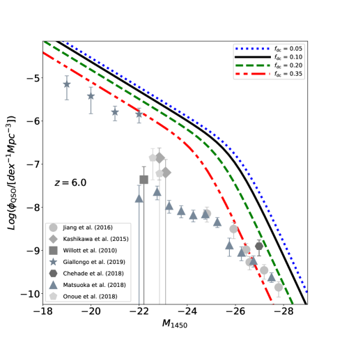
Figure 1: Estimated $z=6$ AGN LF. The predictions from our models are compared with observational constraints. Line types, colours and symbols as indicated in the legends.

Larger $f_{\rm dc}$ values imply a faster LF evolution. Vice-versa, a small duty cycle implies an almost negligible evolution of the space density of luminous sources. Indeed, in our simplified framework and for a given SMBH, a short $f_{\rm dc}$ implies a small probability of being active (and for a short time). Therefore, in order to explain the observed AGN space densities, we need to assume a large number of available SMBHs, most of which are expected to be non-accreting. These “inactive” SMBHs are available for powering AGN of similar luminosities at slightly earlier times. On the other hand, a $f_{\rm dc}\simeq 1$ implies that the observed $z\simeq 5$ AGNs should correspond (almost) to the only available SMBHs of that mass in the Universe.

It is also worth noticing that, for all $f_{\rm dc}$ values, the evolution of the AGN-LF strictly follows the Eddington accretion path: this implies that our estimated evolution qualifies as a pure luminosity evolution, in contrast with the typical pure density evolution scenario often assumed to estimated the LF evolution (see e.g. Kim & Im, 2021). In particular, $f_{\rm dc}>0.2$ scenarios predict a fast drop in the space density of the brightest $M_{1450}<-27.5$ QSOs, which results in a negligible number of these sources at $z\lower 2.15277pt\hbox{$\;\buildrel>\over{\sim}\;$}7$ (assuming that QSOs at $z=5$ and $z=7$ belong to the same parent population and/or the number of detected $z\simeq 7$ QSOs is representative of the total population). On the other hand, if $f_{\rm dc}<0.2$ the space density of bright sources evolves moderately from $z=5$ to $z=7$.

3 Constraining the model with observations

3.1 Luminosity Functions

In order to get a first constraint on our model predictions, in Fig. 1 we compare them with available estimates for $z\simeq 6$ AGN/QSO LF (Willott et al., 2010; Kashikawa et al., 2015; Jiang et al., 2016; Onoue et al., 2017; Chehade et al., 2018; Matsuoka et al., 2018; Giallongo et al., 2019). These data provide us with an estimate for the space densities of active BHs at different luminosities. By focusing at the bright end, we may conclude that $f_{\rm dc}\simeq 0.35$ is a reasonable value that reproduces the available evidence; at the same time, we can exclude larger $f_{\rm dc}$ values that would correspond to a faster than observed $5<z<6$ LF evolution. However, if also $z\simeq 6$ data are subject to relevant incompleteness, as the QUBRICS space densities at $z\simeq 5$ suggest, we can see them as lower limits for the space densities of active BHs, which translates into a $f_{\rm dc}\lower 2.15277pt\hbox{$\;\buildrel<\over{\sim}\;$}0.35$. Therefore, we conclude that the comparison with available constraints on space densities favours $0.35\lower 2.15277pt\hbox{$\;\buildrel<\over{\sim}\;$}f_{\rm dc}\lower 2.15277pt\hbox{$\;\buildrel<\over{\sim}\;$}0.1$.

3.2 Ionizing Backgrounds

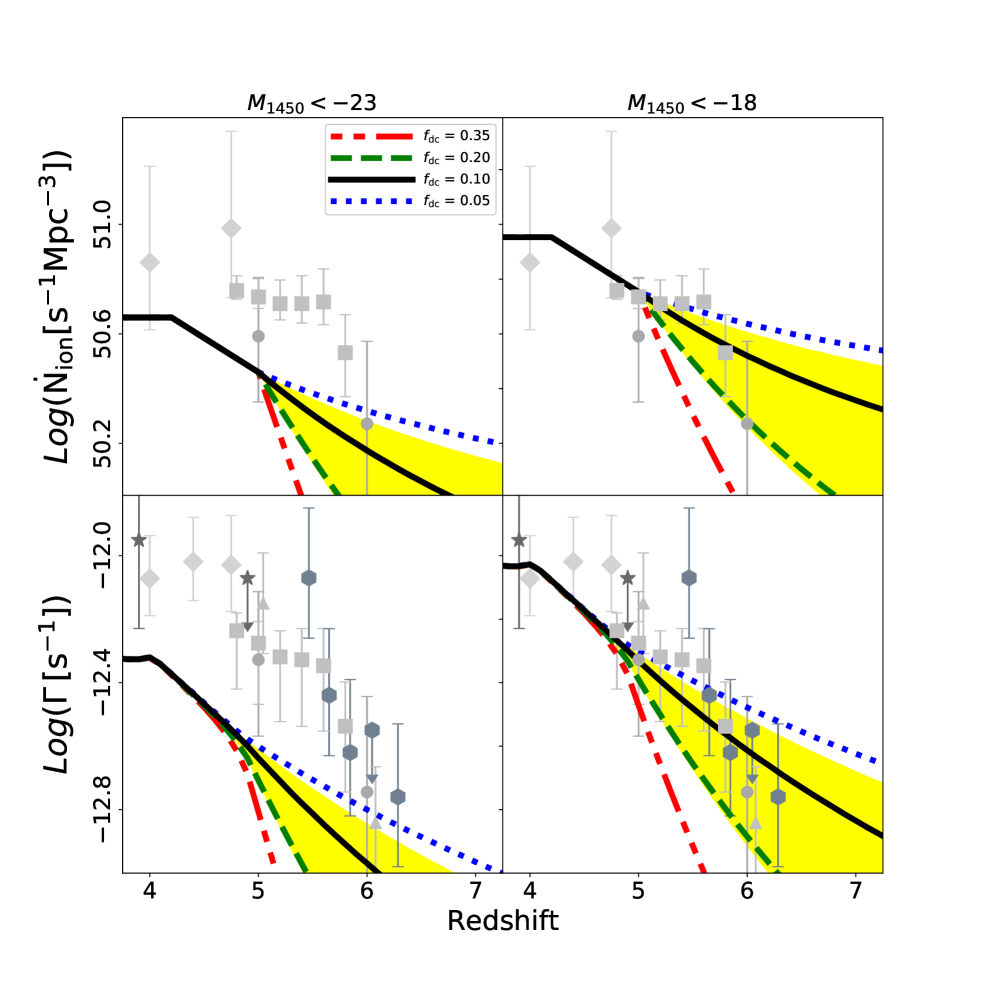
Figure 2: Redshift evolution of the photon volume emissivity ($N_{\rm ion}$ -upper panels) and hydrogen photoionization rate ($\Gamma$ - lower panels). Observed data are from Wyithe & Bolton (2011, circles), Calverley et al. (2011, triangles), Becker & Bolton (2013, diamonds), D’Aloisio et al. (2018, squares), Davies et al. (2018a, hexagons) and Gallego et al. (2021, stars). In all panels, different line-types refer to the predictions of our empirical modelling for different values of the $f_{\rm dc}$ parameter (as indicated in the legend). The yellow shaded area represents the range of predictions for $f_{\rm dc}=0.1$ models with $\epsilon$ ranging from 0.05 to 0.15. Right and left panels refer to different choices of the limiting integration magnitude for the AGN-LF, as indicated in the upper label (see text for a more detailed discussion on our choices for $f_{\rm esc}$ and $M_{\rm lim}$).

Our estimated evolution of the $z>5$ AGN-LF can be translated into a prediction for the AGN contribution to the observed photoionization rate and ionizing photons volume emissivity in the Early Universe (Fig. 2), using the same formalism as described in Cristiani et al. (2016). We summarise the main steps in the following. Following Haardt & Madau (2012), we numerically solved the equations of radiative transfer to get the photoionization rate $\Gamma$:

$$\Gamma(z)=4\pi~{}\int_{\nu_{H}}^{\nu_{\rm up}}\frac{J(\nu,z)}{h_{p}\nu}\sigma_{HI}(\nu)d\nu$$ (2)

In the previous equation, $J(\nu,z)$ is the background intensity computed as:

$$J(\nu,z)=c/4\pi\int_{z}^{\infty}\epsilon_{\nu_{1}}(z_{1})e^{-\tau_{\rm e}}\frac{(1+z)^{3}}{(1+z_{1})^{3}}\,|\frac{dt}{dz_{1}}|\,dz_{1}$$ (3)

where $\tau_{\rm e}(\nu,z,z_{1})$ is the effective opacity between $z$ and $z_{1}$:

$$\tau_{\rm e}(\nu,z,z_{1})=\int_{z}^{z_{1}}dz_{2}\int_{0}^{\infty}dN_{HI}f(N_{HI},z_{2})(1-e^{-\tau_{\rm c}(\nu_{2})})$$ (4)

and $\tau_{\rm c}$ is the continuum optical depth. Moreover we also estimate the comoving density of ionizing photons as:

$$\dot{N}_{\rm ion}(z)=\int_{\nu_{H}}^{\nu_{\rm up}}\frac{\rho_{\nu}}{h_{p}\nu}d\nu$$ (5)

In all previous equations, $\nu_{i}=\nu\frac{1+z_{i}}{1+z}$, $\nu_{H}$ is the frequency corresponding to $912$ Å and $\nu_{\rm up}=4\nu_{H}$; $f(N_{HI},z)$ is the bivariate distribution of absorbers as in Becker & Bolton (2013); $\epsilon_{\nu}(z)$ and $\rho_{\nu}$ represent the proper and comoving volume emissivity (at frequency $\nu$), respectively, that can be computed by integrating the AGN-LF $\Phi(L,z)$, e.g.:

$$\rho_{\nu}=\int_{M_{\rm min}}^{\infty}f^{\rm AGN}_{\rm esc}(L,z)\,\Phi(L,z)\,L_{\nu}(L)\,dL$$ (6)

We assume a universal QSO/AGN broken power-law spectral shape of the form $f_{\nu}\propto\nu^{-\gamma}$: in detail, we use $\gamma=-0.70$ in the wavelength range 500 Å $<\lambda<$ 1000 Å (Shull et al., 2012; Lusso et al., 2015) and $\gamma=-2$ at shorter wavelengths (Telfer et al., 2002). A key parameter is the integration depth, $M_{\rm min}$, which limits the number of sources that are included in the computation. $f_{\rm esc}^{\rm AGN}$ represents the escape fraction (i.e. the fraction of ionizing photons produced by the source that are able to escape the galaxy and ionize the intergalactic medium). In principle, the escape fraction could be a function of both the luminosity of the object and its redshift (as well as of other physical properties). In this paper we consider a fixed $f_{\rm esc}^{\rm AGN}=0.75$ value, based on the Cristiani et al. (2016) estimate for $M_{1450}\lower 2.15277pt\hbox{$\;\buildrel<\over{\sim}\;$}-27.5$ QSOs.

Fig. 2 shows the predicted evolution of the photoionization rate and ionizing photons volume emissivity for different $f_{\rm dc}$ values, ranging from 5 to 35 percent. We present two different scenarios, based on different assumptions for the limiting magnitude. In the left panels, we show a conservative scenario, where we consider only ionizing photons coming from QSOs (i.e. $M_{\rm lim}=M_{1450}<-23$). On the right panel, instead, we discuss the predictions on a more speculative scenario, where we assume that our modelling hold up to $M_{\rm lim}<-18$ and that the derived properties of bright AGNs are representative of objects living on the faint-end of the LF as well. In particular, we consider the same $f_{\rm esc}^{\rm AGN}=0.75$, derived for bright QSOs, over the whole luminosity range, i.e. we imply that fainter AGNs resemble scaled-down versions of the most powerful lighthouses in the Universe. Low-z observations of AGNs around and fainter than the knee of the LF suggest that these sources are not dramatically different from bright counterparts (Stevans et al., 2014; Boutsia et al., 2018; Grazian et al., 2018).

In general, large $f_{\rm dc}\lower 2.15277pt\hbox{$\;\buildrel>\over{\sim}\;$}0.2$ values imply a fast evolution of the AGN-LF and a fast drop of both the photon emissivity and photoionization rate at $z>5$, well below the present available constraints. Similarly, small $f_{\rm dc}<0.1$ correspond to a negligible evolution of the AGN-LF and a flatter evolution for the background. Therefore, intermediate values ($0.05<f_{\rm dc}<0.2$) result in $\dot{N}_{\rm ion}$ and $\Gamma$ predictions that are the most consistent with the observed evolutionary trends. Changing $\epsilon$ within reasonable values (i.e. from 0.05 to 0.15) provides predictions that are qualitatively consistent. The yellow shaded area represents the span of models with fixed $f_{\rm dc}=0.1$ and a variable $\epsilon$ between 0.05 and 0.15 (upper and lower envelope respectively), and it is representative for other $f_{\rm dc}$ choices.

As already shown in our previous work (Boutsia et al., 2021), the relative normalization of predictions and data is tightly linked to the integration depth assumed on the AGN-LF. Moreover, our modelling neglects completely the contribution of star-forming galaxies at comparable redshifts: those sources, although less efficient in producing ionizing photons, have space densities much larger than the AGN population and may supply a relevant contribution to the total ionizing background (Fontanot et al., 2012a; Cristiani et al., 2016). Nonetheless, our modelling for $f_{\rm dc}=0.1$ shows that, if sources fainter than $M_{1450}=-23$ (and up to $M_{1450}<-18$) are taken into account, Eddington-accreting AGNs at $z>5$ can provide enough ionizing photons to account for the observed background. Such a deep integration limit, tied with the assumption that the high $f_{\rm esc}^{\rm AGN}$ observed in the brightest QSO does not dramatically drop for faint AGNs is crucial in our framework. As an alternative interpretation, $M_{\rm lim}$ can be viewed as the limiting magnitude of the AGN population characterized by a $f_{\rm esc}^{\rm AGN}$ comparable to bright QSOs, that is to say that a luminosity dependent $f_{\rm esc}^{\rm AGN}$ prescription would naturally predict an equivalent $M_{\rm lim}$. However, as clearly shown in Fig. 2, both a deep integration of the AGN-LF and a high $f_{\rm esc}^{\rm AGN}$ are required for the AGN population to provide a ionizing photon space density comparable with the estimated background at $z\simeq 5$, which represents the starting point of our analysis.

3.3 Reionization

3.3.1 Modelling of evolution of the ionized fraction

Additional insight on the photon budget in the EoR is provided by the redshift evolution of the neutral fraction of the dominant baryonic components of the Universe, Helium and Hydrogen ($x_{\rm HeIII}$ and $x_{\rm HII}$, respectively). The evolution of the neutral fraction is linked to the corresponding filling factors ($Q_{\rm HeIII}$ and $Q_{\rm HII}$); we model the $Q$ evolution following two different approaches. The first one represents the standard approach in the literature: following Madau et al. (1999), we assume that reionization is an homogeneous process and that $Q$s obey the equation describing the evolution of the filling factors:

$$\dot{Q}=\frac{\dot{N}_{\rm ion}}{\langle n\rangle}-\frac{Q}{\langle t_{\rm rec}\rangle}$$ (7)

where $\dot{N}_{\rm ion}$ is the comoving density of ionizing photons for each species (i.e. between 1 and 4 Rd for Hydrogen, between 4 and 16 Rd for Helium); $\langle n\rangle$ is the mean comoving density of atoms of the considered species (with $\langle n_{\rm He}\rangle=\langle n_{H}\rangle/12.$) and $\langle t_{\rm rec}\rangle$ is the volume-averaged recombination rate of the species (see e.g. Madau & Haardt, 2015):

$$\langle t^{\rm HII}_{\rm rec}\rangle^{-1}=C(z)\,(1+\chi)\,\langle n_{H}\rangle\,\alpha_{\rm HII}(T)\,(1+z)^{3}$$

$$\langle t^{\rm HeIII}_{\rm rec}\rangle^{-1}=C(z)\,Z\,(1+2\chi)\,\langle n_{H}\rangle\,\alpha_{\rm HeIII}(T/Z^{2})\,(1+z)^{3}$$

where $\chi=Y/[4(1-Y)]$ includes photoelectrons from He_II; $Y$ is the primordial Helium mass fraction, $Z=2$ is the ionic charge; $C(z)=2.9[(1+z)/6]^{-1.1}$ is the redshift dependent clumping factor (that we assume being the same for both species) as in Madau & Haardt (2015) and $\alpha$s represent the case B recombination coefficient for H_II and He_III (Hui & Gnedin, 1997):

$$\langle\alpha_{\rm HII}\rangle=2.753\times 10^{-14}\frac{(315614/T)^{1.5}}{\left[1+(115188/T)^{0.407}\right]^{-2.242}}$$

$$\langle\alpha_{\rm HeIII}\rangle=5.506\times 10^{-14}\frac{(1263030/T)^{1.5}}{\left[1+(460960/T)^{0.407}\right]^{-2.242}}$$

In practice, for the purpose of this work, we assume a fixed value for the temperature $T=10^{4}$K, which is appropriate for ionizing regions around QSOs.

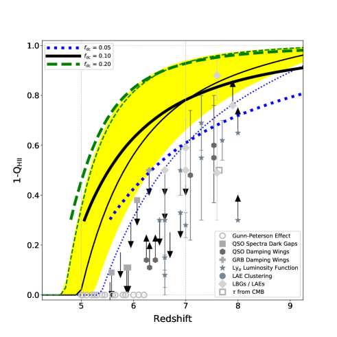
Figure 3: Redshift evolution of the neutral hydrogen fraction. Different line-types and colours refer to the predictions of our empirical modelling for different values of the $f_{\rm dc}$ parameter (as indicated in the legend). Thin and thick line refer to the predictions of the homogeneous and bubble models, respectively (see main text for more details). The yellow shaded area represents the range of predictions for $f_{\rm dc}=0.1$ models with $\epsilon$ ranging from 0.05 to 0.15. Grey symbols show the available observational constraints listed in Table 1.

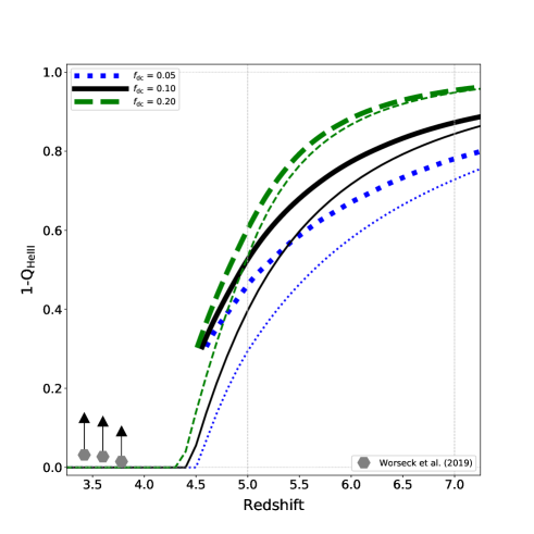
Figure 4: Redshift evolution of the double ionized Helium fraction ($Q_{\rm HeIII}$). Different line-types and colours refer to the predictions of our empirical modelling for different values of the $f_{\rm dc}$ parameter (as indicated in the legend). Thin lines refer to a model assuming homogeneous Helium reionization, while thick lines show the predictions for the bubble model for the evolution of the ionization front of each luminous AGN/QSO (see text for more details). Grey symbols mark the observational determinations by Worseck et al. (2019).

The homogeneous model might not be able to recover some of the details of the reionization process. In particular, the extent of the EoR depends on its topology, i.e. on the spatial distribution of the ionizing sources and their clustering. This is especially important for our hypothesis of an AGN-driven reionization, as AGNs are more sparse and rare sources, with respect, e.g., to star-forming galaxies at comparable redshifts. In order to take these effects into account, while keeping our modelling simple, we develop what we call the “bubble” model. We assume that each AGN develops an (almost) spherical ionized region, and we thus model the evolution of the associated ionization front as a function of its luminosity. Following Khrykin et al. (2016), we assume that an AGN of luminosity $M_{1450}$ is able to affect a spherical volume of radius:

$$R_{\rm IF}(M_{1450})=R_{S}(M_{1450})\left[1-\exp\left(-\frac{t_{\rm lf}}{x_{Q}t_{\rm rec}}\right)\right]^{1/3}$$ (8)

where $R_{S}$ represents the classical Strömgren radius:

$$R_{S}(M_{1450})=\frac{3}{4\pi}\frac{\dot{N}_{\rm ion}(M_{1450})}{\langle n\rangle/t_{\rm rec}}$$ (9)

In the following, we assume that each new QSO episode carves a ionized bubble from a non-ionized medium (i.e. $x_{Q}=1$, which correspond either to a full neutral hydrogen or to a single ionized helium). For the sake of simplicity, we consider a fixed QSO lifetime $t_{\rm lf}$, defined as the $f_{\rm dc}$ fraction of the time interval between $z=5$ and $z=7$. This choice implies that, for $f_{\rm dc}=0.1$, $t_{\rm lf}$ roughly corresponds to a Salpeter time (i.e. 45 Myrs).

At each redshift, we then compute the size of ionized bubbles as a function of $M_{1450}$; by combining the corresponding spherical volumes with the expected space density of sources at that given luminosity, we estimate the volume fraction of the newly ionized medium. We thus change the source term in Eq. 7 with this estimate to test for changes in the $Q$ evolution.

It is worth stressing that the bubble model most likely break down for values of $Q$ approaching unity. Indeed, in our calculations we are implicitly assuming that each new HII (HeIII) bubble starts in an homogeneous neutral (HeII) medium, with no interaction with nearby similar structures. However, for large $Q$ values this is no longer the case, as both physical mechanisms (like bubble percolation) and geometrical considerations (like in the case of AGN clustering, which allows for a QSOs shining in a medium that has been already partially ionized) start to be relevant. As an example, Doussot & Semelin (2022) study the effect of percolation on statistics of ionized bubble size distribution and find that percolation has a relevant effect for $Q>0.7$. It is not easy to assess the effect of these mechanisms on the bubble model. On one hand, both percolation and clustering favour the formation of larger ionization fronts, that should speed up the reionization process (i.e a sharper rise of $Q$ to unity). Nonetheless, if AGN sources are highly clustered, this implies that could exist neutral regions far enough from the closest AGN to be able to survive up to low redshifts. The relative contribution of these two different scenarios is impossible to determine in our simplified approach, so that we prefer to limit the bubble model to $Q<0.7$ in the following analysis.

3.3.2 Hydrogen Reionization

In Fig. 3, we compare the available constraints on $x_{\rm HI}$, coming from different techniques (see Table 1 for detailed references), with the prediction from our homogeneous model (thin lines) for different $f_{\rm dc}$ choices. Fig. 3 clearly shows that in our reference frame only small $f_{\rm dc}$ values are compatible with the data, while larger values require some additional sources of ionizing photons (i.e. star forming galaxies) to close the photon budget. Alternatively, $\epsilon>0.1$ values are required for models with intermediate $f_{\rm dc}\simeq 0.1$ (lower boundary of the yellow region). Wen considering the bubble model, the overall predictions do not change considerably; the largest differences are seen for $f_{\rm dc}<0.2$, with the bubble model predicting slightly more extended EoRs and lower reionization redshifts.

A comparison of Fig. 2 and 3 suggests that, in order to reproduce the $x_{\rm HI}$ evolution, a rather flat and constant $\dot{N}_{\rm ion}$ background is needed (at the level of the observed value at $z\simeq 5$, see also Madau, 2017). In the context of our model that considers only the AGN contribution, such a background can be achieved only with a slowly evolving AGN LF (i.e. $f_{\rm dc}<0.05$ values). Nonetheless, a flat ionizing background seems to be in tension with the available constraints on the photoionization rate at $z\simeq 6$. Such an apparent tension is mainly due to the fact that Eq. 4 holds only for a fully ionized inter-galactic medium. Indeed, Puchwein et al. (2019) show that a more detailed treatment of the effective opacity during the EoR, taking into account the inhomogeneity of the medium (i.e. the presence of regions of neutral hydrogen and helium), leads to a rapid evolution of the mean free path of ionizing photons (Becker et al., 2021). The improved modelling leads naturally to a sharp discontinuity in $\Gamma$ during the EoR, which fits nicely the highest redshift observational determination also in the case of an almost flat background (their Fig. 3).

3.3.3 Helium reionization

A critical test on models for AGN-driven Hydrogen reionization comes from the additional constraints based on the reionization history of the Helium component (see e.g. Furlanetto & Oh, 2008). Helium reionization is believed to be completed by $z\lower 2.15277pt\hbox{$\;\buildrel>\over{\sim}\;$}3$, and sustained by photons above 4 Ry, provided by the growing population of AGNs at $z<4$ (Wyithe & Loeb, 2003). Significant fluctuations of the He_III effective optical depths have been detected at $3<z<4$ (e.g. Worseck et al., 2016, 2019), which cannot be explained by models assuming an uniform mean free path for ionizing photons (Furlanetto & Dixon, 2010) and suggest incomplete Helium reionization at these redshifts (Worseck et al., 2011). Indeed, our homogeneous model predicts relatively early Helium reionization redshifts ($z>4$ - Fig. 4, thin lines), in agreement with, e.g.,Madau & Haardt (2015). On the other hand, the bubble model provides a quite different $Q$ evolution (Fig. 4 - thick lines): with respect to the homogeneous model, for all $f_{\rm dc}$ values, the Helium reionization is more extended and systematically delayed to lower redshifts. These trends decrease for larger $f_{\rm dc}$ due to the fact that they corresponds to larger bubble sizes at fixed luminosity (which thus deviate less from the homogeneous approximation), and the increase in size compensate the smaller space densities associated with the faster LF evolution (Sec. 3.1). It is worth comparing these predictions with recent estimates of QSO lifetimes by Khrykin et al. (2021). They apply Eq. 8 to the analysis of Helium proximity zones in absorption spectra of individual QSOs at $3<z<4$ QSOs, and find that the spectroscopic data are mostly consistent with short lifetimes in the range of $t_{\rm lf}\sim$ 0.5-20 Myr (with a mean value of 1.65 Myr). In the redshift range $5<z<7$, lifetimes $\;\buildrel<\over{\sim}\;$ 20 Myr (i.e. half of a Salpeter time) correspond to $f_{\rm dc}\lower 2.15277pt\hbox{$\;\buildrel<\over{\sim}\;$}0.05$ implying an extended Helium reionization, starting at $z>5$ and being completed at $z<3$.

The most striking difference between the homogeneous and the bubble model for Helium reionization is the systematic drift of $Q$ evolution to lower redshifts at all cosmic epochs, while in the case of Hydrogen reionization the two models provide more similar $Q$ evolutions. It is not easy to understand the origin of this effect, as it is due to a combination of the smaller number of ionizing photons available, the smaller number of HeII atoms and the shorter recombination timescales. We check that our results are robust against reasonable changes in the recombination timescale and clumping factors, which suggests that the smaller comoving density of ionizing photons for Helium with respect to Hydrogen plays the larger role.

3.4 Evolution of high-z BH seeds

Our framework also allows us to explore the predicted distribution of BH masses at $z\lower 2.15277pt\hbox{$\;\buildrel>\over{\sim}\;$}5$ and to check under which conditions it complies with the most recent theoretical expectations for the properties of primordial BH seeds. The Initial Mass Function of BHs (BH-IMF) is expected to have a peak at stellar-like masses (i.e. 10-100 $M_{\odot}$ - light seed BHs) corresponding to the remnants of stellar evolution, including the elusive Population III stars (see e.g. García-Bellido et al., 2021; Sureda et al., 2021). It is important to keep in mind that, in order to reach a $\sim 10^{9}M_{\odot}$ SMBH at $z\simeq 7$, a $\sim$ 100 $M_{\odot}$ Pop III seed BH would need 0.8 Gyrs of Eddington accretion, i.e. $f_{\rm dc}\simeq$1. Nonetheless, the BH-IMF most likely spans the full range of 10-10${}^{6}M_{\odot}$: massive seed BHs may result from the near-isothermal collapse of a chemically pristine massive gas cloud (see e.g. Ferrara et al., 2014), from stellar mergers in ultradense star clusters (Devecchi & Volonteri, 2009), or even being the relic of a primordial BH population (see e.g. Yu & Tremaine, 2002). These very massive seeds may only form in highly biased regions of the Universe, moreover, only a small minority of them are bound to evolve into SMBHs, the others being expected to remain lower-mass BHs at the centre of dwarf satellites (Valiante et al., 2016). Therefore, even these models with such massive seeds seem to require high $f_{\rm dc}$ values to explain the observed $z\simeq 7$ SMBHs (Tanaka & Haiman, 2009). Indeed, the situation is further complicated by the possibility of hyper-Eddington accretion (Inayoshi et al., 2016; Takeo et al., 2018): as a result of a short ($0.2<f_{\rm dc}<0.3$) phase of the order of 500 $\dot{M}_{\rm edd}$ most of the stellar mass remnants would reach masses $\sim$ 2 $\times 10^{5}M_{\odot}$, independently of their initial seed mass, thus providing a larger sample of massive SMBHs available for powering luminous sources at high-z (Inayoshi et al., 2020).

Additional constraints on $f_{\rm dc}$ can be thus derived from considering the predicted evolution for the total BHMF. We derived this quantity from the space density of active SMBHs multiplied by the adequate $f_{\rm dc}$. As a benchmark, we compare our models (Fig. 5) against the BH space densities predicted by the semi-analytic codes like cat (Cosmic Archaeology Tool Trinca et al., 2022, grey squares) and the model proposed by Li et al. (2022). The main differences among the two approaches lies in the assumed starting distribution of light and heavy seeds and in the allowed range of Eddington ratios (most notably Li et al. 2022 require several episodes of Super-Eddington accretion, while the best-fit cat model is Eddington-limited). Despite their differences the two codes provide a consistent prediction for the space density of the more massive BHs in a wide redshift range, while they start to diverge at the low-mass end of the BHMF, with cat predicting sistematically higher space densities.

While the lower space densities at the faint end predicted by the Li et al. (2022) model favour large $f_{\rm dc}\simeq 0.35$ values, our models with $0.1<f_{\rm dc}<0.2$ are mostly consistent with cat over the $6<z<10$ redshift range. Models with larger $f_{\rm dc}$ values start to be in tension with cat already at $z=6$, while models with smaller $f_{\rm dc}$ values tend to overpredict the space density of SMBHs. While interpreting these plots it is also important to keep in mind that we define $f_{\rm dc}$ based on a reference redshift range (that is $5<z<7$); moving outside this range to higher redshifts implies that $f_{\rm dc}$ should be seen as a fixed time interval, more than a time fraction (and in particular $5<z<7$ roughly corresponds to a cosmic time interval ten times the Salpeter time).

4 Conclusions

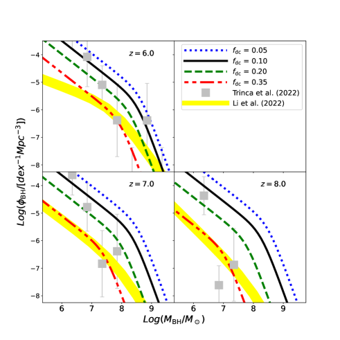
Figure 5: Total (active+inactive) BHMF at $z>5$. Different line-types refer to the predictions of our empirical modelling for different values of the $f_{\rm dc}$ parameter (as indicated in the legend). The grey squares refer to the theoretical predictions for the evolution of direct collapse BHs from Trinca et al. (2022), while the yellow area represents the BHMFs predicted by the model proposed by Li et al. (2022).

We develop an empirical model aimed at studying the redshift evolution of the AGN/QSO-LF under the hypothesis that all SMBHs at $z\lower 2.15277pt\hbox{$\;\buildrel>\over{\sim}\;$}5$ (where we fixed our starting space densities using available estimates) accrete at Eddington rate, which allows us to give redshift estimates also for the BHMF (both for the active and total population). Such a prediction is a fundamental constraint for our approach, since the existence of very massive SMBHs at such high redshift is challenging for current models of early BH “seeding”. The existence of a few $10^{9}M_{\odot}$ SMBHs, powering the observed high-luminosity sources at $z\simeq 7$ (Mortlock et al., 2011; Bañados et al., 2018; Matsuoka et al., 2019; Wang et al., 2021), can be generally reconciled with the expected formation of massive structures at high redshift, by assuming that these are the end product of the rare seeds experiencing very efficient accretion (see e.g. Di Matteo et al., 2012). However, if SMBHs of comparable mass are common also at higher redshifts, their accretion histories are increasingly difficult to reconstruct.

We can roughly divide the predictions of this model into three separate regimes. $f_{\rm dc}\lower 2.15277pt\hbox{$\;\buildrel>\over{\sim}\;$}0.2$ scenarios correspond to fast evolving AGN-LF and negligible space densities of $M_{\rm SMBH}\lower 2.15277pt\hbox{$\;\buildrel>\over{\sim}\;$}10^{8}M_{\odot}$ objects at $z>6$. These models are consistent with conservative estimates for the high-z growth of BH seeds (Tanaka & Haiman, 2009), but they under-predict the space densities implied by more sophisticated models of seed growth (Trinca et al., 2022; Li et al., 2022). Overall, they also predict a vanishing contribution of the AGN population to the observed ionizing background at $z>5$, independently of the integration magnitude $M_{\rm lim}$.

The evolution of the AGN LF for intermediate duty cycles ($f_{\rm dc}\simeq 0.1$) implies BHMFs in good agreement with the expectations of the cat semi-analytic model for the growth of BH seeds in the early Universe. Moreover, they are also able to provide a relevant contribution to the observed ionizing background and photoionization rate, in good agreement with the data, if a deep integration limit ($M_{\rm lim}$) is assumed. Nonetheless, they also predict an important redshift evolution of the AGN space density/ionizing background, which is inconsistent with the observed evolution of the neutral fraction (thus suggesting the need for an additional source of ionizing photons in the EoR).

Finally, $f_{\rm dc}\lower 2.15277pt\hbox{$\;\buildrel<\over{\sim}\;$}0.05$ scenarios feature a slow evolution of the AGN-LF evolution, which correspond to a rather shallow evolution of the ionizing background at high-z. In these models the AGN population alone provides enough ionizing photons to account for the evolution of the Hydrogen neutral fraction. Moreover, such low $f_{\rm dc}$ values imply QSO lifetimes in good agreement with estimates at lower redshift (Khrykin et al., 2021). However, under the hypothesis of homogeneous reionization, such models provide too high redshifts for Helium reionization ($z>4$). We show that a simple model taking into account the topology of reionization (e.g. by following the growth of ionized bubbles around accreting SMBHs) predicts more extended Helium reionization histories, thus easing the tension between AGN-driven Hydrogen reionization scenarios and available data on Helium reionization.

However, the slow evolution of the LF translates into space densities for $M_{\rm SMBH}\sim 10^{8-9}M_{\odot}$ sources relatively high even at $z>6$. Such space densities would be in tension with most models of SMBHs seeding and accretion using Eddington accretion. Nonetheless, these results could be reconciled with theoretical expectations by assuming a relatively short period of super/hyper-Eddington accretion (see also Pezzulli et al., 2016) at $z>7$ that could easily bring a good fraction of the light seed into the $\sim$ 10${}^{5}M_{\odot}$ mass range, thus changing the shape of the highest-z BH-IMF. If such a scenario holds, we may have enough massive SMBH at $5<z<7$ to account for these relatively low duty cycles.

It is extremely difficult to disentangle these scenarios based on the available data, which become sparse at $z\lower 2.15277pt\hbox{$\;\buildrel>\over{\sim}\;$}5$. Our modelling provides a reference frame to investigate the role of AGN/QSO in the EoR, based on a number of assumptions, the most relevant being the idea that the properties of faint sources (most notably their $f_{\rm esc}^{\rm AGN}$) can be derived from their bright QSO counterparts. Starting from this assumption, we could place interesting constraints to the contribution of the AGN population to the photon budget during the EoR: depending on the assumed $M_{\rm lim}$ the AGNs/QSOs move from being a relevant contributor into being the dominant population. This in turn implies that, while waiting for the James Webb Space Telescope to provide unprecedented constraints on the evolution of the high-z AGN-LF, coordinated efforts like QUBRICS represent excellent pathfinders for our understanding of the processes at play in such early epochs.

Data Availability

Predictions for the $z>5$ AGN-LF evolution and/or relative AGN ionizing background for a variety of parameter combinations will be shared on reasonable request to the corresponding author.

Appendix A Neutral fraction estimates

Table 1 collect available estimates for the evolution of the neutral fraction at $z>5$ coming from different techniques (as listed in the title of the different sections).

Table 1: Constraints on $x_{HI}$ from the literature (updated from Bouwens et al. 2015)

Redshift	$x_{HI}$	Reference
Gunn-Peterson Effect (data are in units of $10^{-5}$)
5.03	$5.49^{+1.42}_{-1.65}$	Fan et al. (2006)
5.25	$6.70^{+2.07}_{-2.44}$	”
5.45	$6.77^{+2.47}_{-3.01}$	”
5.65	$8.60^{+3.65}_{-4.60}$	”
5.85	$12.00^{+4.08}_{-4.90}$	”
6.10	$43.^{+30.}_{-30.}$	”
5.40	$5.71^{+0.59}_{-1.21}$	Yang et al. (2020)
5.60	$7.61^{+1.61}_{-0.75}$	”
5.80	$8.8^{+1.8}_{-1.2}$	”
6.00	$11.4^{+5.5}_{-1.9}$	”
6.20	$10.3^{+5.5}_{-1.1}$	”
5	$3.020^{+0.230}_{-0.058}$	Bosman et al. (2021)
5.1	$3.336^{+0.064}_{-0.164}$	”
5.2	$3.636^{+0.131}_{-0.095}$	”
5.3	$3.598^{+0.556}_{-0.145}$	”
Dark Pixel Fraction in Quasar Spectra
5.58	$<0.09$	McGreer et al. (2015)
5.87	$<0.11$	”
6.07	$<0.38^{+0.20}$	”
5.9	$\lower 2.15277pt\hbox{$\;\buildrel<\over{\sim}\;$}0.11$	Greig & Mesinger (2017)
5.55	$<0.05$	Zhu et al. (2022)
5.75	$<0.17$	”
5.95	$<0.29$	”
Ly$\alpha$ Damping Wing (QSOs)
6.247	$\lower 2.15277pt\hbox{$\;\buildrel>\over{\sim}\;$}0.14$	Schroeder et al. (2013)
6.308	$\lower 2.15277pt\hbox{$\;\buildrel>\over{\sim}\;$}0.11$	”
6.419	$\lower 2.15277pt\hbox{$\;\buildrel>\over{\sim}\;$}0.14$	”
7.09	$0.48^{+0.26}_{-0.26}$	Davies et al. (2018b)
7.54	$0.60^{+0.20}_{-0.23}$	”
7.54	$0.55^{+0.21}_{-0.18}$	Bañados et al. (2018)
7.29	$0.49^{+0.11}_{-0.11}$	Greig et al. (2022)

Redshift	$x_{HI}$	Reference
Ly$\alpha$ Damping Wing (GRBs)
6.3	$\leq 0.5$	Totani et al. (2006)
Ly$\alpha$ Luminosity Function
6.5	$\lower 2.15277pt\hbox{$\;\buildrel<\over{\sim}\;$}0.3$	Malhotra & Rhoads (2004)
6.6	$0.08^{+0.08}_{-0.05}$	Morales et al. (2021)
7.0	$0.28^{+0.05}_{-0.05}$	”
7.3	$0.69^{+0.11}_{-0.11}$	”
6.6	$0.3^{+0.2}_{-0.2}$	Konno et al. (2018)
6.6	$0.15^{+0.15}_{-0.15}$	Ouchi et al. (2018)
6.9	$0.4-0.6$	Zheng et al. (2017)
6.9	$<0.33$	Wold et al. (2022)
7.3	$0.55^{+0.25}_{-0.25}$	Konno et al. (2014)
7.7	$0.62^{+0.08}_{-0.08}$	Faisst et al. (2014)
$\sim 8$	$\lower 2.15277pt\hbox{$\;\buildrel>\over{\sim}\;$}0.3$	Tilvi et al. (2014)
8	$>0.65$	Schenker et al. (2014)
6.6	$0.3^{+0.1}_{-0.1}$	Ning et al. (2022)
Ly$\alpha$ Emitting Galaxies / Lyman Break Galaxies
$\sim 7$	$0.59^{+0.11}_{-0.15}$	Mason et al. (2018)
$7.6\pm 0.6$	$0.88^{+0.08}_{-0.10}$	Hoag et al. (2019)
7.6	$0.49^{+0.19}_{-0.19}$	Jung et al. (2020)
$7.9\pm 0.6$	$>0.76$	Mason et al. (2019)
6.6	$<0.4$	Yoshioka et al. (2022)
$6.7\pm 0.2$	$<0.25$	Bolan et al. (2021)
$7.6\pm 0.6$	$0.83^{+0.08}_{-0.11}$	”
Clustering of Ly$\alpha$ Emitting Galaxies
6.6	$<0.5$	Sobacchi & Mesinger (2015)
7.0	$\lower 2.15277pt\hbox{$\;\buildrel<\over{\sim}\;$}0.5$	”
$\tau_{es}$ from CMB
$7.64\pm 0.74$	$0.5$	Planck Collaboration et al. (2020)
9.75	$0.76^{+0.22}_{-0.27}$	Dai et al. (2019)

References

- Bañados et al. (2018) Bañados E., et al., 2018, Nature, 553, 473
- Becker & Bolton (2013) Becker G. D., Bolton J. S., 2013, MNRAS, 436, 1023
- Becker et al. (2021) Becker G. D., D’Aloisio A., Christenson H. M., Zhu Y., Worseck G., Bolton J. S., 2021, MNRAS, 508, 1853
- Bolan et al. (2021) Bolan P., et al., 2021, arXiv e-prints, p. arXiv:2111.14912
- Bosman et al. (2021) Bosman S. E. I., et al., 2021, arXiv e-prints, p. arXiv:2108.03699
- Boutsia et al. (2018) Boutsia K., Grazian A., Giallongo E., Fiore F., Civano F., 2018, ApJ, 869, 20
- Boutsia et al. (2020) Boutsia K., et al., 2020, ApJS, 250, 26
- Boutsia et al. (2021) Boutsia K., et al., 2021, ApJ, 912, 111
- Bouwens et al. (2009) Bouwens R. J., et al., 2009, ApJ, 705, 936
- Bouwens et al. (2015) Bouwens R. J., Illingworth G. D., Oesch P. A., Caruana J., Holwerda B., Smit R., Wilkins S., 2015, ApJ, 811, 140
- Calderone et al. (2019) Calderone G., et al., 2019, ApJ, 887, 268
- Calverley et al. (2011) Calverley A. P., Becker G. D., Haehnelt M. G., Bolton J. S., 2011, MNRAS, 412, 2543
- Chehade et al. (2018) Chehade B., et al., 2018, MNRAS, 478, 1649
- Cristiani et al. (2016) Cristiani S., Serrano L. M., Fontanot F., Vanzella E., Monaco P., 2016, MNRAS, 462, 2478
- D’Aloisio et al. (2018) D’Aloisio A., McQuinn M., Davies F. B., Furlanetto S. R., 2018, MNRAS, 473, 560
- Dai et al. (2019) Dai W.-M., Ma Y.-Z., Guo Z.-K., Cai R.-G., 2019, Phys. Rev. D, 99, 043524
- Davies et al. (2018a) Davies F. B., Hennawi J. F., Eilers A.-C., Lukić Z., 2018a, ApJ, 855, 106
- Davies et al. (2018b) Davies F. B., et al., 2018b, ApJ, 864, 142
- Devecchi & Volonteri (2009) Devecchi B., Volonteri M., 2009, ApJ, 694, 302
- Di Matteo et al. (2012) Di Matteo T., Khandai N., DeGraf C., Feng Y., Croft R. A. C., Lopez J., Springel V., 2012, ApJ, 745, L29
- Doussot & Semelin (2022) Doussot A., Semelin B., 2022, arXiv e-prints, p. arXiv:2208.14044
- Faisst et al. (2014) Faisst A. L., Capak P., Carollo C. M., Scarlata C., Scoville N., 2014, ApJ, 788, 87
- Fan et al. (2006) Fan X., et al., 2006, AJ, 132, 117
- Ferrara et al. (2014) Ferrara A., Salvadori S., Yue B., Schleicher D., 2014, MNRAS, 443, 2410
- Fontanot et al. (2012a) Fontanot F., Cristiani S., Santini P., Fontana A., Grazian A., Somerville R. S., 2012a, MNRAS, 421, 241
- Fontanot et al. (2012b) Fontanot F., Cristiani S., Vanzella E., 2012b, MNRAS, 425, 1413
- Fontanot et al. (2020) Fontanot F., et al., 2020, MNRAS, 496, 3943
- Furlanetto & Dixon (2010) Furlanetto S. R., Dixon K. L., 2010, ApJ, 714, 355
- Furlanetto & Oh (2008) Furlanetto S. R., Oh S. P., 2008, ApJ, 681, 1
- Gallego et al. (2021) Gallego S. G., et al., 2021, MNRAS, 504, 16
- García-Bellido et al. (2021) García-Bellido J., Carr B., Clesse S., 2021, Universe, 8, 12
- Giallongo et al. (2015) Giallongo E., et al., 2015, A&A, 578, A83
- Giallongo et al. (2019) Giallongo E., et al., 2019, ApJ, 884, 19
- Grazian et al. (2018) Grazian A., et al., 2018, A&A, 613, A44
- Grazian et al. (2022) Grazian A., et al., 2022, ApJ, 924, 62
- Greig & Mesinger (2017) Greig B., Mesinger A., 2017, MNRAS, 465, 4838
- Greig et al. (2022) Greig B., Mesinger A., Davies F. B., Wang F., Yang J., Hennawi J. F., 2022, MNRAS, 512, 5390
- Guarneri et al. (2021) Guarneri F., Calderone G., Cristiani S., Fontanot F., Boutsia K., Cupani G., Grazian A., D’Odorico V., 2021, MNRAS, 506, 2471
- Haardt & Madau (2012) Haardt F., Madau P., 2012, ApJ, 746, 125
- Hoag et al. (2019) Hoag A., et al., 2019, ApJ, 878, 12
- Hui & Gnedin (1997) Hui L., Gnedin N. Y., 1997, MNRAS, 292, 27
- Inayoshi et al. (2016) Inayoshi K., Haiman Z., Ostriker J. P., 2016, MNRAS, 459, 3738
- Inayoshi et al. (2020) Inayoshi K., Visbal E., Haiman Z., 2020, ARA&A, 58, 27
- Jiang et al. (2016) Jiang L., et al., 2016, ApJ, 833, 222
- Jung et al. (2020) Jung I., et al., 2020, ApJ, 904, 144
- Kashikawa et al. (2015) Kashikawa N., et al., 2015, ApJ, 798, 28
- Khrykin et al. (2016) Khrykin I. S., Hennawi J. F., McQuinn M., Worseck G., 2016, ApJ, 824, 133
- Khrykin et al. (2021) Khrykin I. S., Hennawi J. F., Worseck G., Davies F. B., 2021, MNRAS, 505, 649
- Kim & Im (2021) Kim Y., Im M., 2021, ApJ, 910, L11
- Konno et al. (2014) Konno A., et al., 2014, ApJ, 797, 16
- Konno et al. (2018) Konno A., et al., 2018, PASJ, 70, S16
- Li et al. (2022) Li W., Inayoshi K., Onoue M., Toyouchi D., 2022, arXiv e-prints, p. arXiv:2210.02308
- Lusso et al. (2015) Lusso E., Worseck G., Hennawi J. F., Prochaska J. X., Vignali C., Stern J., O’Meara J. M., 2015, MNRAS, 449, 4204
- Madau (2017) Madau P., 2017, ApJ, 851, 50
- Madau & Haardt (2015) Madau P., Haardt F., 2015, ApJ, 813, L8
- Madau et al. (1999) Madau P., Haardt F., Rees M. J., 1999, ApJ, 514, 648
- Malhotra & Rhoads (2004) Malhotra S., Rhoads J. E., 2004, ApJ, 617, L5
- Mason et al. (2018) Mason C. A., Treu T., Dijkstra M., Mesinger A., Trenti M., Pentericci L., de Barros S., Vanzella E., 2018, ApJ, 856, 2
- Mason et al. (2019) Mason C. A., et al., 2019, MNRAS, 485, 3947
- Matsuoka et al. (2018) Matsuoka Y., et al., 2018, ApJ, 869, 150
- Matsuoka et al. (2019) Matsuoka Y., et al., 2019, ApJ, 872, L2
- McGreer et al. (2015) McGreer I. D., Mesinger A., D’Odorico V., 2015, MNRAS, 447, 499
- Merloni & Heinz (2008) Merloni A., Heinz S., 2008, MNRAS, 388, 1011
- Morales et al. (2021) Morales A. M., Mason C. A., Bruton S., Gronke M., Haardt F., Scarlata C., 2021, ApJ, 919, 120
- Mortlock et al. (2011) Mortlock D. J., et al., 2011, Nature, 474, 616
- Ning et al. (2022) Ning Y., Jiang L., Zheng Z.-Y., Wu J., 2022, ApJ, 926, 230
- Onoue et al. (2017) Onoue M., et al., 2017, ApJ, 847, L15
- Onoue et al. (2022) Onoue M., et al., 2022, arXiv e-prints, p. arXiv:2209.07325
- Ouchi et al. (2018) Ouchi M., et al., 2018, PASJ, 70, S13
- Pezzulli et al. (2016) Pezzulli E., Valiante R., Schneider R., 2016, MNRAS, 458, 3047
- Planck Collaboration XVI (2014) Planck Collaboration XVI 2014, A&A, 571, A16