MAFUS: a Framework to predict mortality risk in MAFLD subjects

Abstract

Metabolic (dysfunction) associated fatty liver disease (MAFLD) establishes new criteria for diagnosing fatty liver disease independent of alcohol consumption and concurrent viral hepatitis infection. However, the long-term outcome of MAFLD subjects is sparse. Few articles are focused on mortality in MAFLD subjects, and none investigate how to predict a fatal outcome. In this paper, we propose an artificial intelligence-based framework named MAFUS that physicians can use for predicting mortality in MAFLD subjects. The framework uses data from various anthropometric and biochemical sources based on Machine Learning (ML) algorithms. The framework has been tested on a state-of-the-art dataset on which five ML algorithms are trained. Support Vector Machines resulted in being the best model. Furthermore, an Explainable Artificial Intelligence (XAI) analysis has been performed to understand the SVM’s diagnostic reasoning and the contribution of each feature to the prediction. The MAFUS framework is easy to apply, and the required parameters are readily available in the dataset.

1 Introduction

Nonalcoholic Fatty Liver Disease (NAFLD) is the leading cause of chronic liver disease in Western countries, as well as a condition raising the risk for cardiovascular diseases, type $2$ diabetes mellitus and chronic renal disease, and increased mortality  Fazel et al. (2016); Levene and Goldin (2012). The prevalence of NAFLD is estimated at $24\%$ worldwide (from $15\%$ in $2005$ to $25\%$ in $2010$). A meta-analysis published in $2016$ reported an average prevalence of $23.71\%$ in Europe Younossi et al. (2016). Population-based studies conducted in our geographical area (district of Bari, Apulian Region, Italy), are estimated a NAFLD prevalence of around $30\%$, mainly among male subjects and older people Cozzolongo et al. (2009). NAFLD is defined as an accumulation of high triglycerides in the hepatocytes ($>5\%$ of the liver volume), after excluding viral infectious causes or other specific liver diseases Neuschwander-Tetri and Caldwell (2003). NAFLD can manifest as fatty liver disease (hepato-steatosis) or as non-alcoholic steatohepatitis (NASH). An evolution of the former in which steatosis comes with inflammation, hepatocellular injury, and fibrogenic activation may lead to cirrhosis and hepatocarcinogenesis. MAFLD is a novel concept proposed in $2020$ aiming to replace the term NAFLD Eslam et al. (2020a). Unlike NAFLD, MAFLD does not require the exclusion of other etiologies of liver disease, such as excessive alcohol consumption or viral hepatitis Eslam et al. (2020b). MAFLD is diagnosed in subjects who have both hepatic steatosis and one of the following three metabolic diseases: overweight/obesity (Subtype 1), evidence of Metabolic Dysregulation (MD) in lean subjects (Subtype 2), or diabetes mellitus (Subtype 3) Eslam et al. (2020c).

In addition, it is unclear whether the new definition provides better detectability regarding hard clinical endpoints (e.g., mortality). Although ample evidence of the association of MAFLD with Cardiovascular Diseases (CVD), malignancies, and liver-related endpoints, the impact on mortality remains controversial Semmler et al. (2021).

In recent years, due to the increasing prevalence of NAFLD and a new definition of MAFLD, there is a research trend toward identifying low-cost diagnostic methods, and ML is acknowledged as a valuable method. In clinical practice, numerous works have shown how ML or e-health tools are considered various alternatives to standard diagnostic methods Casalino et al. (2021); Castellana et al. (2022); Lella et al. (2021); Casalino et al. (2022) such as Magnetic Resonance Imaging (MRI), ultrasounds, etc. ML approaches are already used for NAFLD diagnosis Sorino et al. (2020, 2021).

According to Curci et al. Curci et al. (2022) who demonstrated the benefits of Physical Activity and Diet intervention in subjects with MAFLD, in this paper, we propose a method to predict the patient’s outcome (Mortality (Yes/No)), in order to allow the physician, to suggest a lifestyle modification (Diet and Physical Activity) to the subjects when Mortality (Yes) is predicted.

The experimental setup is designed on a population-based cohort after $15$ years of follow-up. A dataset containing $25$ variables is used in the experiments. A feature relevance analysis is performed to identify the features correlated to the target variable.

To determine an optimal method for predicting mortality in MAFLD subjects, we compare ML algorithms based on readily available laboratory variables for accuracy, precision, recall, F1 score, and confusion matrix. As a result, we developed a system for accurately predicting mortality based on biochemical and anthropometric parameters in a cohort of MAFLD subjects so that the clinician understood the rationale for the system’s predictions (Mortality (Yes/No).

Explainability analysis is used to highlight the characteristics Mortality (Yes) versus Mortality (No) with relative final prediction to support the physician’s decision.

The remainder of the paper is organized as follows: in Section 2 we overview the most relevant related work;
Section 3 describes the proposed approach and Section 4 reports the metrics used to measure the performance of our model and the explanation obtained from the XAI analysis. FInally, Section 5 tightens the conclusion and future research directions.

2 Related work

In this section, we reviewed the state of the art on the MAFLD condition and clarified the significant differences between this study and existing work by highlighting the innovative contribution of this study. Dan-Qin Sun et al. Sun et al. (2021) investigated the distribution of MAFLD and NAFLD subjects and the majority of these two groups of individuals with Chronic Kidney Disease (CKD). This study aimed to compare CKD prevalence in MAFLD or NAFLD subjects and the association between the presence and severity of MAFLD and CKD and abnormal albuminuria. The authors evidenced that the severity of renal dysfunction and the prevalence of CKD stage $1$ increased progressively with the severity of MAFLD. The results of this study suggest that MAFLD better identifies subjects with CKD than NAFLD and that both MAFLD with elevated liver fibrosis scores are strongly and independently associated with CKD and abnormal albuminuria. Compared to our work, the authors do not consider mortality to train an Artificial intelligence (AI) algorithm and do not perform any explainability analysis to support physician activities.

Su Lin et al. Lin et al. (2020) proposed a comparison of MAFLD and NAFLD diagnostic criteria to validate the diagnostic criteria of MAFLD. This study aims to compare the characteristics of MAFLD and NAFLD. They compared clinical parameters of MAFLD, NAFLD, and non-MD-NAFLD subjects, highlighting statistically significant differences. The main findings are that MAFLD criteria can distinguish more at-risk subjects. The MAFLD population had higher liver enzymes and more glucose and lipid metabolism disorders than NAFLD. Compared to our study, the authors focused only on validating the diagnostic criteria of MAFLD. They did not investigate additional aspects of the disease and explainability, such as those addressed in our study.

Decraecker et al. Decraecker et al. (2022) suggested an evaluation of non-invasive methods in MAFLD subjects. This study aims to develop non-invasive prognostic methods to predict mortality. The authors developed several prognostic models for survival and outcome and compared the prognostic accuracy of all methods considered. The study showed that non-invasive assessment of liver fibrosis at baseline was correlated with all-cause mortality and liver-related mortality in MAFLD subjects. A predictive model (consisting of clinical parameters and measurement of liver stiffness, Fibrosis-4 (FIB-4) or LIVERFASt) was an excellent predictor of all-cause mortality and liver-related mortality (C-index $\approx 0.8-0.9$) and a good predictor of all-cause and liver-related outcomes (AUC $\approx 0.72-0.74$) in MAFLD.

Compared to our study, the authors focused on developing different prognostic models for survival and identifying the best predictive model for mortality in MAFLD subjects. However, the authors did not use variables readily available in healthcare databases to develop these models.

They did not use mortality and readily available variables to train an AI algorithm and explainability analysis that can help physicians in the decision-making process in MAFLD subjects.

Nguyen et al. Nguyen et al. (2021) propose a study examining the baseline characteristics and long-term outcomes of three different groups of participants with ultrasound-defined fatty liver disease. These groups are those who meet the criteria for NAFLD, but not MAFLD (non-MAFLD NAFLD), those who meet the requirements for both NAFLD and MAFLD (NAFLD-MAFLD), and those who meet the criteria for MAFLD but not NAFLD (MAFLD non-NAFLD). The authors highlight that non-NAFLD MAFLD was independently associated with all-cause mortality compared with non-MAFLD NAFLD. In summary, persons meeting diagnostic criteria for MAFLD but not NAFLD are most likely to have advanced fibrosis. They had the highest all-cause, CVD-related, and other-cause mortality compared with those meeting the criteria for NAFLD but not MAFLD or those with both NAFLD and MAFLD. MAFLD subjects without NAFLD have more than twice the risk of mortality compared with those with NAFLD without MAFLD.

They did not investigate the mortality to train an AI algorithm that can assist physicians in predicting mortality in MAFLD subjects. In addition, no explainability analysis is considered.

Kim et al. Kim et al. (2021) developed a Cox proportional hazards model to study all-cause mortality and cause-specific mortality between MAFLD and NAFLD, with adjustments for known risk factors. The study aimed to investigate the independent longitudinal association of NAFLD and MAFLD on all-cause and cause-specific mortality in US adults. The authors highlighted that all-cause mortality risk was higher for subjects with advanced fibrosis and MAFLD than those with advanced fibrosis and NAFLD. There was a strong association between MAFLD and all-cause mortality. MAFLD had a $17\%$ higher risk of all-cause mortality with statistical significance, whereas NAFLD showed no association with all-cause mortality after adjustment for metabolic risk factors. These findings suggest that MAFLD is strongly associated with all-cause mortality, independently of known metabolic risk factors. Compared to our study, the authors focused on analyzing the independent longitudinal association of NAFLD and MAFLD on all-cause and cause-specific mortality.

The authors do not perform any AI algorithm to train readily available variables to predict mortality and do not consider explainability analysis to assist physicians in MAFLD decision-making.

Huanget al. Huang et al. (2021) investigated an evaluation of the closest association with all-cause and cause-specific mortality in MAFLD and NAFLD subjects and that drug development for MAFLD should consider ethnic differences. The authors divided the participants into four groups for survival analysis: without NAFLD or MAFLD, with NAFLD only, and MAFLD only. MAFLD increased the overall risk of all-cause mortality more than NAFLD. The risks of cardiovascular, neoplastic, and diabetes-related mortality are similar between MAFLD and NAFLD. Compared with individuals without NAFLD and MAFLD, individuals with NAFLD alone showed a reduction in total mortality and neoplasm mortality in crude. However, individuals with only MAFLD independently increased the risk of total mortality and neoplasm mortality. The risk of all-cause mortality in MAFLD was consistent among subgroups, except for race-ethnicity and whether secondary to viral hepatitis. MAFLD showed a higher risk of all-cause mortality and equal risk of cause-specific mortality than NAFLD.

Compared to our study, the authors focused on investigating the association between all-cause and cause-specific mortality in MAFLD and NAFLD subjects. They also suggest that development for MAFLD should consider ethnic differences. They did not investigate mortality using variables readily available in the health dataset to train AI algorithms, and they did not perform any explainability analysis to support physicians.

To sum up, the discussion above confirms that despite several contributions to state-of-the-art, none of them analyze and evaluate the proposed techniques for predicting mortality in MAFLD subjects and driving the physician in the decision-making process. The present work represents an advancement of state of the art by introducing a novel approach to predict mortality in MAFLD subjects and using explainability techniques.

3 The proposed approach

This section describes the framework, the data used, and the proposed method to perform and explain the mortality prediction in MAFLD subjects.

3.1 Developing a Framework for mortality prediction in MAFLD subjects

In this work, a framework is proposed to classify MAFLD subjects. Then explainability techniques are applied to justify the algorithmic reasoning. The following considerations drive the choice of experimental set in contributions: (i) to intervene early with treatment, physicians need to identify which subjects are at high mortality risk, and (ii) physicians must understand how the algorithm predicts the target variable.

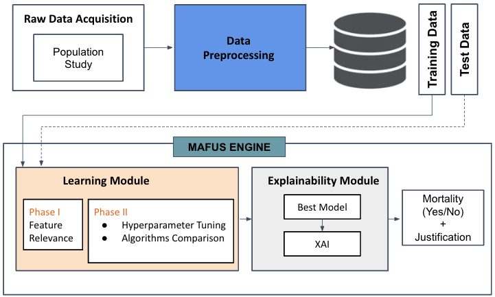
The framework is depicted in Figure 1. The data preparation consists of the following steps: (i) acquisition of data from a population study (Section 3.2) and, (ii) preprocessing operation concerning data cleaning and standardization.

To classify the data, the framework works as follows. For each sample, there are $24$ features and the mortality status. An attribute selection tool is used to select relevant and informative attributes.

Following the data preprocessing, a ready-to-use dataset is obtained. Subsequently, the dataset is divided into training and test sets using the standard 80/20 method.

Our framework is developed around the MAFUS engine composed of two macro-components: (i) the Learning Module that learns and takes care of the prediction part through the use of ML techniques and (ii) Explainability Module that interprets the previous model results to justify and better explain the final result. A hyperparameter tuning is performed using a grid search technique. The output of the explainability module is the result of the best model classification, with the addition of an explanation based on the post-hoc approach.

Figure 1: MAFUS classification framework.

According to Algorithm  1, missing values are removed before starting the training step. A complete subset of the data is obtained and then split into train and test sets. An iterative process follows, in which the algorithm is trained, and then predictions are made. A description of the operations performed by the algorithm is also provided. In the second part of the pseudocode we have two conditions: (i) if the predicted outcome is equal to $0$ (Mortality (No)), the sample is added to set $\mathcal{A}$; (ii) if it is equal to $1$ (Mortality (Yes)), the sample is added to set $\mathcal{B}$. In both cases, the SHAP-based explanation is computed.

By the end of the process, the framework is able to predict whether the patient will be Mortality (no) or Mortality (Yes). In addition, MAFUS  highlights the algorithmic reasoning and the contribution of each feature to the prediction. Pseudocode 1 summarizes the different steps of MAFUS  framework.

Function: • $Clean\text{ }$ removes the missing values contained in $D_{train}$ and $D_{test}$; • $\phi_{i}(f,x)$ shapley values related for each feature;

Input:

• $N$ number of dataset observations;

• $N_{train}$ number of observation in training set

• train and test datasets $D_{train}$ and $D_{test}$, where $D_{train}=\{\mathcal{X}_{train},\mathcal{Y}_{train}\}$, and $D_{test}=\{\mathcal{X}_{test},\mathcal{Y}_{test}\}$;

• target label Classifier = $f(\cdot)$;

• SHAP value generator $\phi(f,x_{i})$ = $<$$S_{1},$…$,S_{z}$$>$, where $z$ is the number of features;

Result:

• $\hat{y}$ represents the prediction;

• set $\mathcal{A}$ composed of tuples of subjects related to the samples associated with a Mortality (No) (i.e., $f(\mathbf{x})=0$);

• set $\mathcal{B}$ composed of tuples of subjects related to the samples associated with a Mortality (Yes) (i.e., $f(\mathbf{x})=1$);

• $Shapley_{values}$ = $\bigcup_{i=1}^{D_{test}}\phi(f,x_{i})$;

$Preprocessing$

for $n\leftarrow 1$ to $N$ do

       $Clean\text{ }D_{train}$ and $D_{test}$;

      

endfor

$\mathcal{X}_{train},\mathcal{Y}_{train}\leftarrow D_{train}$;

for $n\leftarrow 1$ to $N_{train}$ do

       $\mathcal{\hat{Y}}_{train}\leftarrow f(\mathcal{X}_{train})$;

endfor

for $d^{(i)}\in D_{test}$ do

       $\mathbf{x}^{(i)},y^{(i)}\leftarrow d^{(i)}$;

       $\hat{y}^{(i)}\leftarrow f(\mathbf{x}^{(i)})$;

       $Shapley_{values}\leftarrow Shapley_{values}\cup\phi(f,x_{i})$;

endfor

if $\hat{y}^{(i)}=0$ then

      $\mathcal{A}\cup\{\langle\mathbf{x}^{(i)},\phi_{i}(f,x),\hat{y}^{(i)}\rangle\}$ ;

      

end if

else

       $\mathcal{B}\cup\{\langle\mathbf{x}^{(i)},\phi_{i}(f,x),\hat{y}^{(i)}\rangle\}$;

      

end if

Algorithm 1 Algorithm for model training and SHAP evaluation of MAFUS.,

3.2 Population study and clinical data collection

The population cohort consisted of $1,674$ subjects aged $>30$ years ($543$ women and $1131$ men) affected by MAFLD at recruitment from participants in the second follow-up of the MICOL cohort and the NUTRIHEP cohort Mirizzi et al. (2021), recruited from January 2005 and followed until December $31$, $2020$. The baseline characteristics of the subjects are detailed in supplementary Table LABEL:tab:baseline_tab.

The studies have been performed at the National Institute of Gastroenterology, and the ”S. De Bellis” Research Hospital in Castellana Grotte (Italy), and each participant signed an informed consent form. All procedures are performed according to the ethical standards of the institutional research committee (MICOL study: DDG-CE-$589$/$2004$, DDG-CE-$782$/$2013$; NUTRIHEP study, DDG-CE-$502$/$2005$, and DDG-CE-$792$/$2014$) and with the $1964$ Helsinki declaration.

Participants are interviewed to collect information on sociodemographic characteristics, health status, personal history, tobacco use, dietary intake, education level, employment, and marital status. Weight is measured with an electronic scale, SECA mechanical balance, and height with a wall-mounted stadiometer, SECA. Blood pressure and BMI are measured according to international guidelines  Sever (2006). The central hospital’s laboratory collected and processed fasting venous blood according to standard procedures Organization et al. (2010). All subjects underwent standardized ultrasonography performed by two radiologists using a Hitachi H21 Vision machine (Hitachi Medical Corporation, Tokyo, Japan) and a 3.5 MHz transducer. Steatosis is dichotomously classified as absent or present.

3.3 The dataset

Subjects under study had $25$ features containing continuous or categorical values of biochemical, anthropometric, and sociodemographic variables. Specifically, the $25$ columns contained the values of: Aspartate aminotransferase (AST), Weight, Hypertension, Blood lipids, Systolic blood pressure (SBP), Diastolic Blood Pressure (DBP), Total Cholesterol (TC), Triglycerides, Blood Glucose, Alkaline Phosphatase, High-Density Lipoprotein Cholesterol (HDL-C), Low-Density Lipoprotein Cholesterol (LDL-C), Alanine aminotransferase (ALT), Glutamyltransferase (GGT), Age, HOMA-IR Index (HOMA), Residual Cholesterol, Body Mass Index (BMI) as continuous variables, and Status (Mortality (No), Mortality (Yes)), Education, Job, Marital Status, Diabetes condition, Smoke, Gender as categorical variables. The dataset is represented by tabular data composed of $1,674$ observations and $25$ features, including the target variable. The Supplementary Table 1 in Appendix described the characteristics of the population under study.

3.4 Data pre-processing and features relevance analysis

We parsed the dataset using a well-known Python framework, pandas and removed all missing values.

After the missing-values removal, the number of subjects is $1,561$. These observations are standardized according to the StandardScaler technique, known in the ML literature Gadekallu et al. (2020) for reducing variance within datasets. Therefore, they are used to perform a feature selection analysis exploiting Extreme Gradient Boosting (XGBoost) classifier.

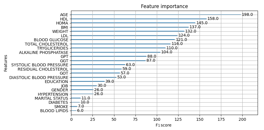
As a result of adopting the XGBoost classifier for feature selection, we evaluated each feature’s F1 score value to determine which contributed most to the prediction. After this selection, the features described in the previous Section are considered. The target variable considered is Status, reported as a binary variable ($0$ = Mortality (No), $1$ = Mortality (Yes)). All biochemical markers are introduced into the models as continuous variables to better reflect their natural scale.

The following nine features are identified according to their contribution, and we selected those with F1 score $>$105: Age, HDL-C, HOMA, BMI, Weight, LDL-C, Blood Glucose, Total Cholesterol, Triglycerides. Furthermore, Gender feature is added for biological importance. Let us consider that, even if gender gets an F1 score $<$105, we added it to the feature set since in the medical domain it is considered a characteristic variable particular in liver disease Lonardo et al. (2019); Hashimoto and Tokushige (2011).

Figure 2 shows the ranking of the features according to their relevance. F1 score is used to describe how each feature contributes to predicting the target variable.

Figure 2: Contribution of each feature measured in terms of F1 score.

3.5 Classification models

In order to determine the best classifier to predict the mortality in MAFLD subjects, we used the following models: Multilayer Perceptron (MLP) Baxt (1995); Random Forest (RF) Pal (2005); Support Vector Machine (SVM) Noble (2006); Extreme Gradient Boosting (XGBoost) Chen et al. (2015); Light Gradient Boosting Machine (LGBM) Fan et al. (2019);

The models are developed with Python, using Scikit-learn v$1.1.2$ library.The following metrics are detailed in the next Section: percentage accuracy, Receiver Operating Characteristics (ROC), precision, recall, and F1 score. All these five algorithms are compared to determine the best suited to predict mortality in MAFLD subjects (Section 4).

3.6 Explainability techniques

A post-hoc XAI approach Došilović et al. (2018) is used to explain how the features contribute to predicting the target variable. When prediction and explanation models are combined, there is an unavoidable trade-off between accuracy and simplicity of interpretation. This difficulty is solved by the notion of XAI. XAI tools like Local Interpretable Model-Agnostic Explanations (LIME) Ribeiro et al. (2016) and Shapley Additive exPlanations (SHAP) Lundberg and Lee (2017) are able to explain independently from the predictive model. This study uses SHAP to interpret the feature contribution to the prediction. As reported by Lombardi et al. Lombardi et al. (2022), we suppose that $D$ is a dataset of samples $D=\left[\left(x_{1},y_{1}\right),\left(x_{2},y_{2}\right),\ldots,\left(x_{z},y_{z}\right)\right]$, where $x_{i}$ represents the feature vector for sample $i$ and $y_{i}$ represents the label for sample $i$. Assume that $f$ is a classifier, and $f_{x_{i}}$ is the prediction for the test instance $i$, which corresponds to the predicted label. The goal is to explain the contribution of each feature $j$ among the $S$ features as the average marginal contribution of the feature value across all possible coalitions, i.e., , all possible sets of feature values with and without the feature $j$. Specifically, a coalition, $F$, is defined as a subset of $S,F\subseteq S$. Assuming $f_{x_{i}}(F)$ is the prediction for $f_{x_{i}}$ given $F$, the following equation represents the marginal contribution from adding $j$-th feature value to $F$:

$$\left[f_{x_{i}}(F\cup j)-f_{x_{i}}(F)\right]$$ (1)

To compute the exact Shapley value, all possible subsets of feature values excluding the $j$-th feature value $F\subseteq S-\{j\}$ have to be considered:

$$\phi(f,x)=\sum_{F\subseteq S-\{j\}}\frac{\lvert F\rvert!(\lvert S\rvert-\lvert F\rvert-1)!}{\lvert S\rvert!}\left[f_{x_{i}}(F\cup j)-f_{x_{i}}(F)\right]$$ (2)

where $\lvert F\rvert!$ represents the number of permutations of feature values positioned before the $\mathrm{j}$-th feature, $(\lvert S\rvert-\lvert F\rvert-1)!$ represents the number of permutations of feature values that appear after the $\mathrm{j}$-th feature value, and $\lvert S\rvert!$ is the total number of permutations Lundberg and Lee (2017). The value of $\phi(f,x)$, is called SHAP value of a single feature and, is equivalent to the Shapley value in game theory Lundberg and Lee (2017). The Shapley value is a value that indicates each player’s participation in a cooperative game with numerous players. SHAP calculates the Shapley value of each feature as a player in the learned model. SHAP values are computed for all feature combinations, which requires exponential time. The results of post-hoc explanation analysis applied in this paper are shown in Section 4.3.

4 Experimental results

This section presents and discusses our model’s experimental evaluation results for mortality prediction in MAFLD subjects.

Dataset Splitting. The dataset is split into train and test sets by the standard $80/20$ method. For reproducibility purposes, we used Scikit-learn implementation to split with a random seed set to 1.

Decision-Maker Hyperparameter Tuning and optimization. The adopted classifiers, i.e. MLP, RF, SVM, XGBoost and, LGBM described in Section 3.5, are tuned using a grid search exploration strategy with a $5$-fold cross-validation strategy. Due to the imbalanced nature of the datasets concerning the sensitive classes, the models optimizing the F1 score are chosen (Equation 6). The list of explored hyperparameter values, for reproducibility, is reported in Table 1.

Table 1: Hyperparameter list, values, and type for the classification models reported in this work.

Algorithm	Hyperparameter	Values	Type
Multilayer Perceptron	seed	{1}	Integer
	hidden_layer_sizes	{(sp_randint.rvs(100, 600, 1),	Intger
		sp_randint.rvs(100, 600, 1),
		sp_randint.rvs(100, 600, 1))}
	activation	{tanh, relu, lbfgs}	String
	solver	{sgd, adam, lbfgs}	String
	alpha	{0.0001, 0.001, 0.01, 0.1, 0.9}	Float
	learning_rate	{constant, adaptive}	String
Random Forest	seed	{1}	Integer
	n_estimators	{100, 200, 300, 400, 500}	String
	max_features	{auto, sqrt, log2}	String
	max_depth	{80, 90, 100, 110, 120, 130, 140, 150, None}	String
	criterion	{gini, entropy}	String
	class_weight	{balanced}	String
Support Vector Machines	seed	{1}	Integer
	class_weight	{balanced}	String
	kernel	{rbf, linear}	String
	gamma	{1, 0.1, 0.001, 0.0001}	Float
eXtreme Gradient Boosting	seed	{1}	Integer
	gamma	{1, 0.1, 0.01, 0.001, 0.0001}	Float
	learning_rate	{0.0001, 0.001, 0.01, 0.1, 1}	Float
	max_depth	{3, 21, 3}	Integer
	colsample_bytree	{1/10.0 for i in range(3,10)}	Float
	reg_alpha	{1e-5, 1e-2, 0.1, 1, 10, 100}	Float
Light Gradient Boosting	seed	{1}	Integer
	learning_rate	{0.1, 0.05}	Float
	num_leaves	{3, 10, 31, 50, 100, 200}	Integer
	reg_alpha	{None, 0.01, 0.05, 0.1}	Float
	colsample_bytree	{0.6, 0.8, 1}	Float
	max_depth	{-1, 3, 5, 8, 10}	Integer
	reg_lambda	{None, 0.01, 0.02, 0.03}	Float
	n_estimators	{50, 100, 300}	Integer

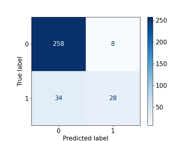
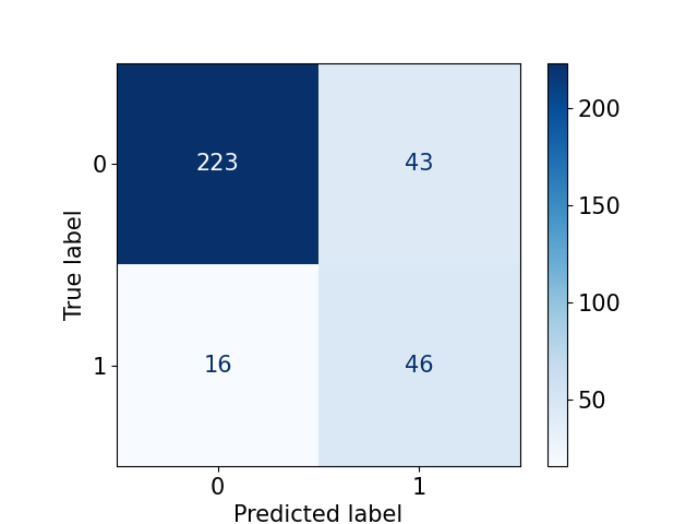
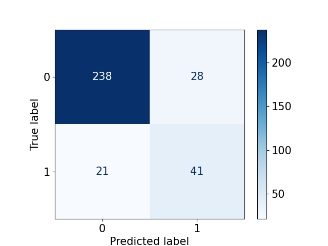
In order to identify the best predictive model, we compared the different algorithms in terms of the metrics reported in Section 4.1. Table 2 shows the performance of each algorithm in predicting mortality. In addition, the Confusion Matrix (CM) is evaluated in Figure 3, to highlight the number of subjects misclassified during the testing phase.

Table 2: Results for the mortality prediction of the compared algorithms.
No/Yes indicate mortality condition.

		Classifier
		RF	XGB	MLP	LGBM	SVM
Precision	No	0.88	0.92	0.88	0.90	0.93
	Yes	0.78	0.59	0.69	0.74	0.52
Recall	No	0.97	0.89	0.95	0.95	0.84
	Yes	0.45	0.66	0.47	0.56	0.74
F1 score	No	0.92	0.91	0.92	0.93	0.88
	Yes	0.57	0.63	0.56	0.64	0,61
Accuracy		0.87	0.85	0.86	0.88	0.82
AUC		0.88	0.85	0.90	0.89	0.90

(a) Confusion Matrix of MLP Classifier.

(b) Confusion Matrix of RF Classifier.

(c) Confusion Matrix of SVM Classifier.

(d) Confusion Matrix of XGB Classifier.

(e) Confusion Matrix of LGBM Classifier.

Figure 3: Representation of confusion matrix values when testing LGBM, MLP, RF, SVM and XGB classifiers. $0$ = Mortality (No), $1$ = Mortality (Yes).

4.1 Evaluation metrics

In this Section, accuracy-based metrics are introduced. They are mainly based on the CM. The first metric is Accuracy, which quantifies the overall ratio of correct classifications for the whole dataset:

$$Accuracy=\frac{TP+TN}{TP+TN+FP+FN}$$ (3)

where $TP$, $TN$, $FP$, and $FN$ represent the number of true positive, true negative, false positive, and false negative predictions, respectively. The Recall metric measures the ratio of correct positive classifications among the total number of positive samples:

$$Recall=\frac{TP}{TP+FN}$$ (4)

The Precision measures the ratio of correct positive classifications among the total positive classifications:

$$Precision=\frac{TP}{TP+FP}$$ (5)

The F1 score is the harmonic mean between recall and accuracy:

$$F1=\frac{2}{\frac{1}{\text{ Precision }}+\frac{1}{\text{ Recall }}}=2\cdot\frac{\text{ Precision }\cdot\text{ Recall }}{\text{ Precision }+\text{ Recall }}$$ (6)

The F1 score combines precision and recall into a single metric. This metric is useful when dealing with imbalanced data. The Area Under the Receiver Operating Characteristic Curve (AUC) is a metric that measures the capability of a classifier to separate the positive class from the negative one. It is formulated as follows: where $X^{+}$ is the set of positive samples, $X^{-}$ is the set of negative samples, $f(\cdot)$ is the result of model prediction, and $\mathbbm{1}(\cdot)$ an indicator function Calders and Jaroszewicz (2007).

4.2 Best model performance evaluation

In this experimental session, we compared the performances of the classifiers. As we can observe in Figure 3(b) and Table 2, RF obtains the highest value of recall ($0.97$), the least number of misclassified in the prediction of class Mortality(No), and the best value of precision, in the prediction of Mortality(Yes)($0.78$). However, the algorithm is not able to correctly discriminate subjects in the Mortality (Yes) class, resulting the worst for this task. LGBM obtains the best value of F1 score in predicting both classes Mortality(No)($0.93$); Mortality(Yes) ($0.64$), the best value of accuracy on the test set ($0.88$) and good discriminative power in predicting Mortality (Yes). MLP, on the other hand, obtains the best AUC value ($0.90$) with the SVM algorithm. However, MLP as RF cannot correctly discriminate subjects belonging to Mortality (Yes). XGB, while performing well on average, does not provide any preponderant metrics compared to the other algorithms. However, it is very balanced and has good discriminative power in predicting Mortality (Yes). SVM instead obtains the best recall values in predicting Mortality (Yes) ($0.74$), the best precision value in predicting Mortality (No) ($0.93$), and is the algorithm with the best discriminative power in predicting Mortality (Yes) as well as having the highest AUC (along with MLP). The goal was to maximize the F1 score in predicting Mortality (Yes) class as the dataset was unbalanced, and we wanted to minimize the number of misclassified in Mortality (Yes). However, as discussed earlier, although LGBM provided the highest F1 score (in the prediction Mortality (Yes)) of $0.64$ (Table 2), we found that SVM is better in predicting Mortality (Yes) than other algorithms, despite having a $0.61$ lower F1 value than LGBM. Since the main goal of this work is to be accurate in identifying subjects with the highest mortality risk in order to allow the physician to intervene early with the lifestyle-change recommendations, the model with the smallest number of errors in predicting Mortality (Yes) is the best. Accordingly, SVM that shows 16 samples misclassified (cfr. Figure 3(c)) is our best choice.

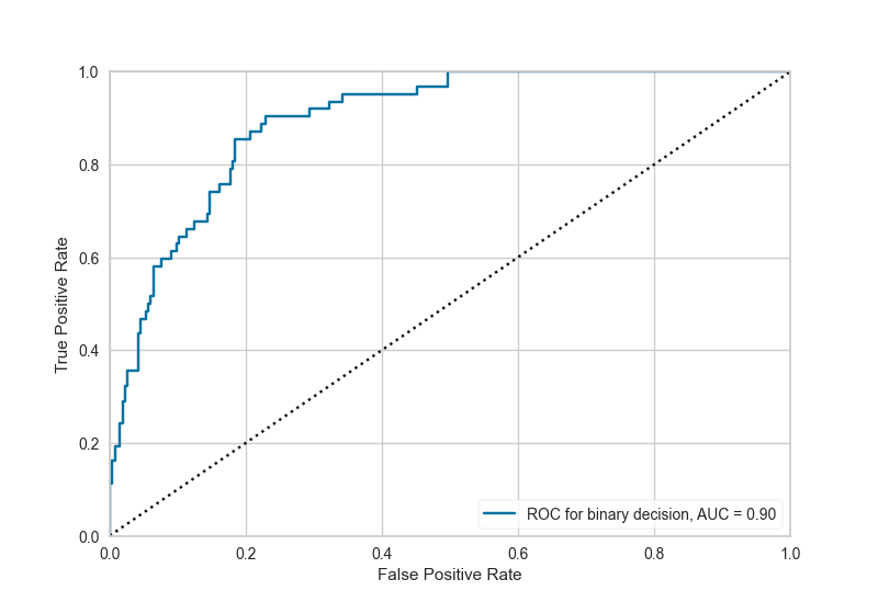
Figure 4 shows the ROC curve with an AUC of $0.90$ obtained from SVM testing. As a measure of accuracy, the area under the ROC (AUC) is used to estimate the test’s discriminant power.

In particular, SVM has a high AUC, which indicates that Mortality (No) and Mortality (Yes) are correctly classified.

Figure 4: Representation of ROC curve and AUC SVM during the test.

4.3 Explainability results

We perform an XAI analysis on the best model results to summarize what we briefly described above. XAI analysis aims to analyze and compare the model’s detection (or decision) strategy to increase trust and understand algorithmic reasoning and contributions of each feature to prediction. XAI analysis is carried out using Python’s SHAP library, after checking the behavior of the SVM (Section 4.2).

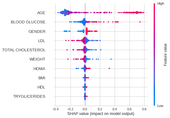
Figure 5 shows the synthesis global diagram using Shapley values of anthropometric and biochemical parameters. There is a relationship between the importance of features and their effects.

The position on the $y$-axis is determined by the feature while on the $x$-axis by the Shapley value, as detailed in Section 3.6. From low to high, from blue to red respectively, the color represents the value of the feature. By jittering overlapping points along the y-axis, we obtained a sense of the distribution of Shapley values across features. In particular, the synthesis global diagram illustrates the following:

• Feature Selection: variables ranked in descending order of importance;

• Impact: horizontal position shows whether the effect of that value is associated with a higher or lower prediction;

• Value: color shows whether that variable is high or low for that observation. The red color means high values and the blue low values. The change in color of the dot shows the value of the feature;

• Correlation: shows the relationship of each characteristic with the target variable.

We assume the direction of Shapley to be independent of XGboost ranking. Shapley values are required to provide the prediction direction from the clinical perspective.

As shown in Figure 5, in our experiments the $Age$ feature is the most important, while the $Triglyceride$ feature is the least important.

Figure 5: Representation of shaply values of anthropometric and biochemical parameters considered.

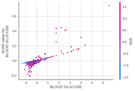
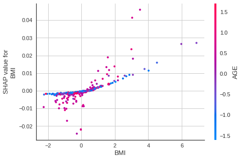
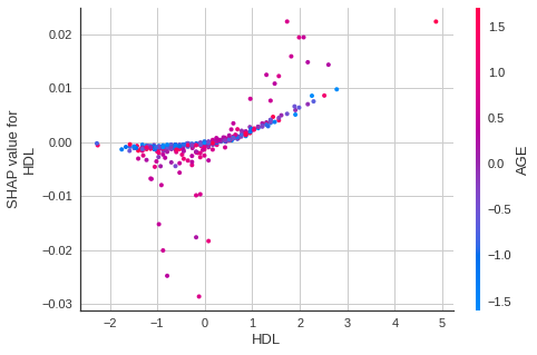
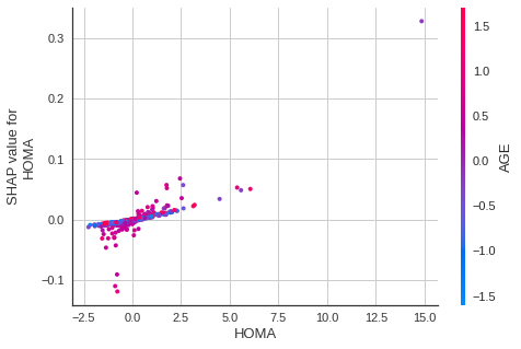
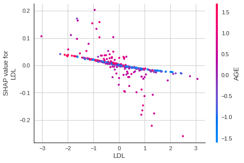
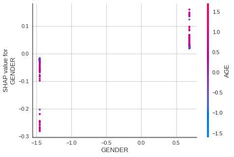
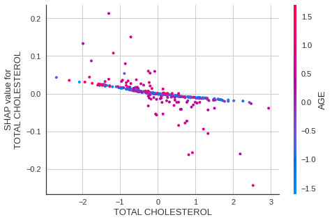
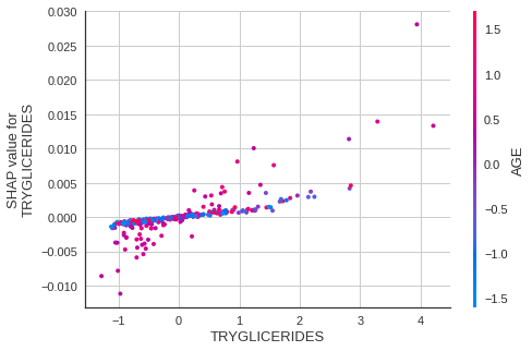
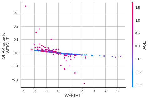
After identifying $Age$ as the most significant feature in the prediction, a study of the dependence of SHAP features is conducted, analyzing the dependencies between all other features and $Age$. SHAP dependence graphs show the expected results of a method. In this way, you can show how a feature affects model output, thus demonstrating the model’s dependence on it. More specifically in a SHAP dependence graph:

• Each dot is a single prediction (row) from the dataset;

• x-axis is the value of the feature (from the $X$ matrix);

• y-axis is the SHAP value for that feature, which represents how much knowing that feature’s value changes the output of the model for that sample’s prediction.

• By default, the color corresponds to a second feature that may interact with the feature we are plotting. If an interaction effect is present between this other feature and the feature we are plotting it will show up as a distinct vertical pattern of coloring.

Figures 6 and 7 show the dependence of each feature. Specifically, we evaluated the most indicative features. They are illustrated below.

According to Figure 7(c), similar features on the x-axis have different impacts on prediction. As the age of the male increases (Value on the x-axis $>$ $0.5$), the prediction shifts toward Mortality (Yes).

In Figures 6(a), 6(b),  6(c),  7(a),  7(b),  7(d), 7(e),  7(f) it is shown that low values of features on the x-axis and high values of features on y-axis contribute to predicting Mortality (No). As the x and y-axes of the feature increase, Mortality (Yes) becomes more of a contributor to the prediction. The x-axis also shows a similar value for features with different impacts on prediction.

(a) Dependence plot of Blood Glucose vs. Age SHAP value in MAFUS.

(b) Dependence plot of BMI vs. Age SHAP value in in MAFUS.

(c) Dependence plot of HDL vs. Age SHAP value in in MAFUS.

Figure 6: Representation of dependence plot for AGE vs. BLOOD GLUCOSE, BLOOD GLUCOSE vs. AGE and, BMI and HDL vs. AGE (the feature with largest contribution in the prediction).

(a) Dependence plot of HOMA vs. Age SHAP value in in MAFUS.

(b) Dependence plot of LDL vs. Age SHAP value in in MAFUS.

(c) Dependence plot of Gender vs. Age SHAP value in MAFUS.

(d) Dependence plot of Total Cholesterol vs. Age SHAP value in in MAFUS.

(e) Dependence plot of Tryglicerides vs. Age SHAP value in MAFUS.

(f) Dependence plot of Weight vs. Age SHAP value in MAFUS.

Figure 7: Representation of dependence plot for HDMA, LDL, GENDER and TOTAL CHOLESTEROL, TRYGLICERIDES and, WEIGHT vs. AGE (the feature with largest contribution in the prediction).

In addition, we observe how the SVM algorithm worked by randomly selecting two subjects from the Mortality (No) and Mortality (Yes) classes, and obtaining a prediction that verifies $No$ and $Yes$ respectively.

Figure 8 displayed the positive and negative SHAP values on the left and right sides as if competing against each other. In particular, it shows which characteristics had a greater impact on a prediction of Mortality (Yes).

Figure 8: Application of SHAP for prediction of Mortality (Yes) during the test.

As shown in Figure 8, the characteristics $Gender$ and $Age$ are both positive predictors, whereas $Blood$ $Glucose$ is negative.

Figure 9 shows which characteristics had a greater on a prediction of Mortality (No).

Figure 9: Application of SHAP for prediction of Mortality (No) during the test.

As shown in Figure 9, the feature $Gender$, the set of features $Age$, $Blood$ $Glucose$, $LDL$, $Weight$ and, $Total$ $Cholesterol$ have a positive and negative impact on the prediction, respectively.

5 Conclusion and further directions

This research proposes a framework to classify mortality in MAFLD subjects. The framework consists of two main components: an $AIAnalysis$ module and a $XAIAnalysis$, both based on machine learning techniques (MLTs). As part of this work, we compared various machine learning algorithms to determine which is best at predicting mortality among MAFLD subjects.

In all cases, the algorithms under study performed well in terms of accuracy. A good F1 score and the lowest number of misclassifications for the Mortality (Yes) class are considered when choosing the best algorithm. XGboost, LGBM, and SVM had the best F1 scores with $0.62$, $0.64$, and $0.61$ respectively.

According to the results (Section 4), SVM produced the fewest prediction errors in the testing phase, despite having a lower accuracy and F1 score than XGboost and LGBM.

To determine the mortality risk in MAFLD subjects, an SVM is trained and explained so that the clinician can understand how the algorithm came to the prediction. Identifying subjects with target variable $1$ (Mortality (Yes)) is the goal to allow the physician to intervene early with lifestyle-change recommendations (suggesting Diet and Physical Activity) according to Curci et al. Curci et al. (2022).

It is important to note that the dataset used for training and testing ML algorithms is unbalanced and contains a few subjects classified as Mortality (Yes). This unbalanced dataset does not allow the algorithm to predict this class well. Another limitation is that no MAFLD mortality classifier has been developed in other studies, so we cannot compare our results to other baselines.

The novelty of the proposal, as well as its remarkable properties and flexibility, has the potential to pave the way for further research.

In future work, Deep Learning (DL) algorithms will be assessed and analyzed in relation to the prediction of mortality in MAFLD subjects. In addition, other approaches based on feature relevance can be studied. Other datasets will be studied to predict mortality in MAFLD subjects, especially local ones, where the proposed method can be applied. The number of observations in the dataset used in the study will be increased, and a DL algorithm will be developed to increase predictive performance. Subsequently, a web-based application based on ML/DL algorithm may be developed in order to provide an easy-to-use tool for the physician.

Acknowledgments This work was partial support of the projects: Italian P.O. Puglia FESR 2014 – 2020 (project code $6$ESURE$5$) ‘SECURE SAFE APULIA’, Fincons CdP3, PASSPARTOUT, Servizi Locali 2.0, ERP4.0. We thanks to Micol and Nutriep group. We thank Dr. Alberto Rubén Osella for authorizing the use of the data.

References

- Fazel et al. (2016) Y. Fazel, A. B. Koenig, M. Sayiner, Z. D. Goodman, Z. M. Younossi, Epidemiology and natural history of non-alcoholic fatty liver disease, Metabolism 65 (2016) 1017–1025.
- Levene and Goldin (2012) A. P. Levene, R. D. Goldin, The epidemiology, pathogenesis and histopathology of fatty liver disease, Histopathology 61 (2012) 141–152.
- Younossi et al. (2016) Z. M. Younossi, A. B. Koenig, D. Abdelatif, Y. Fazel, L. Henry, M. Wymer, Global epidemiology of nonalcoholic fatty liver disease—meta-analytic assessment of prevalence, incidence, and outcomes, Hepatology 64 (2016) 73–84.
- Cozzolongo et al. (2009) R. Cozzolongo, A. R. Osella, S. Elba, J. Petruzzi, G. Buongiorno, V. Giannuzzi, G. Leone, C. Bonfiglio, E. Lanzilotta, O. G. Manghisi, et al., Epidemiology of hcv infection in the general population: a survey in a southern italian town, Official journal of the American College of Gastroenterology ACG 104 (2009) 2740–2746.
- Neuschwander-Tetri and Caldwell (2003) B. A. Neuschwander-Tetri, S. H. Caldwell, Nonalcoholic steatohepatitis: summary of an aasld single topic conference, Hepatology 37 (2003) 1202–1219.
- Eslam et al. (2020a) M. Eslam, A. J. Sanyal, J. George, A. Sanyal, B. Neuschwander-Tetri, C. Tiribelli, D. E. Kleiner, E. Brunt, E. Bugianesi, H. Yki-Järvinen, et al., Mafld: a consensus-driven proposed nomenclature for metabolic associated fatty liver disease, Gastroenterology 158 (2020a) 1999–2014.
- Eslam et al. (2020b) M. Eslam, S. K. Sarin, V. W.-S. Wong, J.-G. Fan, T. Kawaguchi, S. H. Ahn, M.-H. Zheng, G. Shiha, Y. Yilmaz, R. Gani, et al., The asian pacific association for the study of the liver clinical practice guidelines for the diagnosis and management of metabolic associated fatty liver disease, Hepatology international 14 (2020b) 889–919.
- Eslam et al. (2020c) M. Eslam, P. N. Newsome, S. K. Sarin, Q. M. Anstee, G. Targher, M. Romero-Gomez, S. Zelber-Sagi, V. W.-S. Wong, J.-F. Dufour, J. M. Schattenberg, et al., A new definition for metabolic dysfunction-associated fatty liver disease: An international expert consensus statement, Journal of hepatology 73 (2020c) 202–209.
- Semmler et al. (2021) G. Semmler, S. Wernly, S. Bachmayer, I. Leitner, B. Wernly, M. Egger, L. Schwenoha, L. Datz, L. Balcar, M. Semmler, et al., Metabolic dysfunction-associated fatty liver disease (mafld)—rather a bystander than a driver of mortality, The Journal of Clinical Endocrinology & Metabolism 106 (2021) 2670–2677.
- Casalino et al. (2021) G. Casalino, G. Castellano, A. Consiglio, N. Nuzziello, G. Vessio, Microrna expression classification for pediatric multiple sclerosis identification, Journal of Ambient Intelligence and Humanized Computing (2021) 1–10.
- Castellana et al. (2022) F. Castellana, S. Aresta, P. Sorino, I. Bortone, D. Lofù, F. Narducci, T. Di Noia, E. Di Sciascio, R. Sardone, An artificial neural network model to assess nutritional factors associated with frailty in the aging population from southern italy, in: 2022 IEEE International Conference on Systems, Man, and Cybernetics (SMC), 2022, pp. 3228–3233.
- Lella et al. (2021) E. Lella, A. Pazienza, D. Lofù, R. Anglani, F. Vitulano, An ensemble learning approach based on diffusion tensor imaging measures for alzheimer’s disease classification, Electronics 10 (2021) 249.
- Casalino et al. (2022) G. Casalino, G. Castellano, G. Zaza, Evaluating the robustness of a contact-less mhealth solution for personal and remote monitoring of blood oxygen saturation, Journal of Ambient Intelligence and Humanized Computing (2022) 1–10.
- Sorino et al. (2020) P. Sorino, M. G. Caruso, G. Misciagna, C. Bonfiglio, A. Campanella, A. Mirizzi, I. Franco, A. Bianco, C. Buongiorno, R. Liuzzi, et al., Selecting the best machine learning algorithm to support the diagnosis of non-alcoholic fatty liver disease: A meta learner study, PLoS One 15 (2020) e0240867.
- Sorino et al. (2021) P. Sorino, A. Campanella, C. Bonfiglio, A. Mirizzi, I. Franco, A. Bianco, M. G. Caruso, G. Misciagna, L. R. Aballay, C. Buongiorno, et al., Development and validation of a neural network for nafld diagnosis, Scientific Reports 11 (2021) 1–13.
- Curci et al. (2022) R. Curci, A. Bianco, I. Franco, A. Campanella, A. Mirizzi, C. Bonfiglio, P. Sorino, F. Fucilli, G. Di Giovanni, N. Giampaolo, et al., The effect of low glycemic index mediterranean diet and combined exercise program on metabolic-associated fatty liver disease: A joint modeling approach, Journal of Clinical Medicine 11 (2022) 4339.
- Sun et al. (2021) D.-Q. Sun, Y. Jin, T.-Y. Wang, K. I. Zheng, R. S. Rios, H.-Y. Zhang, G. Targher, C. D. Byrne, W.-J. Yuan, M.-H. Zheng, Mafld and risk of ckd, Metabolism 115 (2021) 154433.
- Lin et al. (2020) S. Lin, J. Huang, M. Wang, R. Kumar, Y. Liu, S. Liu, Y. Wu, X. Wang, Y. Zhu, Comparison of mafld and nafld diagnostic criteria in real world, Liver international 40 (2020) 2082–2089.
- Decraecker et al. (2022) M. Decraecker, D. Dutartre, J.-B. Hiriart, M. Irles-Depé, F. Chermak, J. Foucher, V. de Lédinghen, Long-term prognosis of patients with metabolic (dysfunction)-associated fatty liver disease by non-invasive methods, Alimentary Pharmacology & Therapeutics 55 (2022) 580–592.
- Nguyen et al. (2021) V. H. Nguyen, M. H. Le, R. C. Cheung, M. H. Nguyen, Differential clinical characteristics and mortality outcomes in persons with nafld and/or mafld, Clinical Gastroenterology and Hepatology 19 (2021) 2172–2181.
- Kim et al. (2021) D. Kim, P. Konyn, K. K. Sandhu, B. B. Dennis, A. C. Cheung, A. Ahmed, Metabolic dysfunction-associated fatty liver disease is associated with increased all-cause mortality in the united states, Journal of hepatology 75 (2021) 1284–1291.
- Huang et al. (2021) Q. Huang, X. Zou, X. Wen, X. Zhou, L. Ji, Nafld or mafld: which has closer association with all-cause and cause-specific mortality?—results from nhanes iii, Frontiers in medicine 8 (2021).
- Mirizzi et al. (2021) A. Mirizzi, L. R. Aballay, G. Misciagna, M. G. Caruso, C. Bonfiglio, P. Sorino, A. Bianco, A. Campanella, I. Franco, R. Curci, et al., Modified wcrf/aicr score and all-cause, digestive system, cardiovascular, cancer and other-cause-related mortality: A competing risk analysis of two cohort studies conducted in southern italy, Nutrients 13 (2021) 4002.
- Sever (2006) P. Sever, New hypertension guidelines from the national institute for health and clinical excellence and the british hypertension society, Journal of the Renin-Angiotensin-Aldosterone System 7 (2006) 61–63.
- Organization et al. (2010) W. H. Organization, et al., WHO guidelines on drawing blood: best practices in phlebotomy, World Health Organization, 2010.
- Gadekallu et al. (2020) T. R. Gadekallu, N. Khare, S. Bhattacharya, S. Singh, P. K. R. Maddikunta, G. Srivastava, Deep neural networks to predict diabetic retinopathy, Journal of Ambient Intelligence and Humanized Computing (2020) 1–14.
- Lonardo et al. (2019) A. Lonardo, F. Nascimbeni, S. Ballestri, D. Fairweather, S. Win, T. A. Than, M. F. Abdelmalek, A. Suzuki, Sex differences in nonalcoholic fatty liver disease: state of the art and identification of research gaps, Hepatology 70 (2019) 1457–1469.
- Hashimoto and Tokushige (2011) E. Hashimoto, K. Tokushige, Prevalence, gender, ethnic variations, and prognosis of nash, Journal of gastroenterology 46 (2011) 63–69.
- Baxt (1995) W. G. Baxt, Application of artificial neural networks to clinical medicine, The lancet 346 (1995) 1135–1138.
- Pal (2005) M. Pal, Random forest classifier for remote sensing classification, International journal of remote sensing 26 (2005) 217–222.
- Noble (2006) W. S. Noble, What is a support vector machine?, Nature biotechnology 24 (2006) 1565–1567.
- Chen et al. (2015) T. Chen, T. He, M. Benesty, V. Khotilovich, Y. Tang, H. Cho, K. Chen, et al., Xgboost: extreme gradient boosting, R package version 0.4-2 1 (2015) 1–4.
- Fan et al. (2019) J. Fan, X. Ma, L. Wu, F. Zhang, X. Yu, W. Zeng, Light gradient boosting machine: An efficient soft computing model for estimating daily reference evapotranspiration with local and external meteorological data, Agricultural water management 225 (2019) 105758.
- Došilović et al. (2018) F. K. Došilović, M. Brčić, N. Hlupić, Explainable artificial intelligence: A survey, in: 2018 41st International convention on information and communication technology, electronics and microelectronics (MIPRO), IEEE, 2018, pp. 0210–0215.
- Ribeiro et al. (2016) M. T. Ribeiro, S. Singh, C. Guestrin, ” why should i trust you?” explaining the predictions of any classifier, in: Proceedings of the 22nd ACM SIGKDD international conference on knowledge discovery and data mining, 2016, pp. 1135–1144.
- Lundberg and Lee (2017) S. M. Lundberg, S.-I. Lee, A unified approach to interpreting model predictions, Advances in neural information processing systems 30 (2017).
- Lombardi et al. (2022) A. Lombardi, D. Diacono, N. Amoroso, P. Biecek, A. Monaco, L. Bellantuono, E. Pantaleo, G. Logroscino, R. De Blasi, S. Tangaro, et al., A robust framework to investigate the reliability and stability of explainable artificial intelligence markers of mild cognitive impairment and alzheimer’s disease, Brain informatics 9 (2022) 1–17.
- Calders and Jaroszewicz (2007) T. Calders, S. Jaroszewicz, Efficient auc optimization for classification, in: European conference on principles of data mining and knowledge discovery, Springer, 2007, pp. 42–53.