Deep Conditional Measure Quantization

Abstract

Quantization of a probability measure means representing it with a finite set of Dirac masses that approximates the input distribution well enough (in some metric space of probability measures). Various methods exists to do so, but the situation of quantizing a conditional law has been less explored. We propose a method, called DCMQ, involving a Huber-energy kernel-based approach coupled with a deep neural network architecture. The method is tested on several examples and obtains promising results.

1 Introduction

1.1 Conditional measure quantization : motivation

In general terms, quantization is the process of replacing a set of values (possibly an infinity of them) with a finite number chosen to be the most representative according to some metric. This is related to vector quantization (?; ?) that operate on objects in a high dimensional space. Applications range from signal processing (?; ?; ?) to finance (?; ?; ?), statistics (?; ?), which makes it an important area of research in statistics, knowledge representation and machine learning. We will be concerned with a particular instance of this question, namely the quantization of probability measures; in this case we want to represent the knowledge encoded into a probability measure $\mu$ with support in $\mathcal{Y}$ by a sum of $Q$ Dirac masses $\delta^{\beta}_{\mathbf{y}}=\sum_{q=1}^{Q}\beta_{q}\delta_{y_{q}}$, where $y_{q}\in\mathcal{Y}$ are chosen such that the distance between $\mu$ and $\delta^{\beta}_{\mathbf{y}}$ is as small as possible (we will come back later to the definition of the distance); here $\beta$ are some weight parameters (see section  2).

But, there are times when $\mu$ is depending itself on another parameter $\mu=\mu_{x}$ or $\mu$ can be a conditional law. The main question treated in this paper is how to compute efficiently the quantization $\mu_{x}$ of the law $\mu$ conditional to $x$. Our proposal is to involve a deep neural network that minimizes the Huber-energy statistical distance (see (?) for a definition) and outputs the quantized version of the conditional law.

The outline of the paper is the following: in the rest of this section we recall some related works from the literature; we present some theoretical information in section 2; the practical implementation of the method is described in sections 3 and 4 together with numerical results. Concluding remarks are the object of section 5.

1.2 Brief literature review on measure quantization, conditional sampling and conditional quantization

In the general area of (non-conditional) measure quantization, a related proposal (?) investigates the Nystrom mean embeddings, that constructs the quantization based on the exploitation of a small random subset of the dataset.

The literature on general conditional quantization is very scarce, but some works have been done in connection to the so called ’conditional $L^{1}$ median . Several works such as (?; ?) ask the question of the conditional $L^{1}$ median; our approach is similar to that one, with the difference that we look for a general quantization, not only a quantization with a single ($Q=1$) point and we are not attached to the first order moment. See also (?) for a proposal involving neural network computations of conditional quantiles.

In a related work, Zhou et al. (?) propose a generative approach to sample from a conditional distribution by learning a conditional generator. They exploit a Kullbak-Liebler (KL) divergence formulation (in (?) a ’energy’ kernel is used instead) but the generator itself is not quantized.

On the contrary, Vuong et al. (?) learn a deep discrete representation using the Wasserstein distance but their approach is not targeted towards conditional distribution representation.

In signal processing, conditional quantization goes often by the name of conditional vector quantization and has been used e.g. for speech encoding in (?), see also (?; ?; ?) for other references in the signal processing area. Our approach differs by choosing to treat the question in a general, not application dependent way which materializes into the choice of the Huber-energy statistical distance and the use of deep neural networks (hereafter called ’DNN’) for interpolation.

Natural language processing is also an application domain; for instance, even if neither GPT-3 (?; ?)  nor its follow-up ChatGPT (?) are designed explicitly as quantizers, in practice ChatGPT will answer based on a user question or previous conversation. Put it otherwise, it selects a small set of possible answers from the conditional probability of any text given previous contents. This is indeed a conditional quantization.

Interpolation by deep neural networks

The conditional quantization, or quantization depending on some parameter, can also be viewed as some kind of interpolation. Given a set of parameters $x_{1},...,x_{L}$ we can pre-compute the quantized conditional distribution for these parameters and then, for any new choice of the parameter, interpolate using the precomputed data.

Several works explored the use of DNNs for interpolation, for instance in (?) a DNN is trained to learn a mapping from input data points to output data points; then, at the prediction time the DNN can generate an interpolated value for any intermediate input value; the applications range from image processing (?) to audio interpolation (?); in (?) data interpolation was used in scientific simulations such as weather forecasting and fluid dynamics simulations.

Other approaches to using DNNs for interpolation involve using the DNN to learn a probabilistic model of the data (?), and generate the interpolated values using the learned data distribution (with applications to natural language processing and time series analysis). In NLP the possibility of language models to learn to infill (missing parts of) text (?) can also be considered close to a extrapolation method.

2 The deep neural network conditional quantization method

2.1 Setting and notations

We follow the usual notation with lowercase letter for values, upper case for random variables and bold face for vectors. Let $\mathcal{X}=\mathbb{R}^{n_{x}}$, $\mathcal{Y}=\mathbb{R}^{n_{y}}$ (with $n_{x}$, $n_{y}$ non-null integers)  and $\mu$ a joint law with support in $\mathcal{X}\times\mathcal{Y}$. Denote $\mu^{X}$ and $\mu^{Y}$ the marginals of the law $\mu$; for instance, if $X$ and $Y$ are two random variable with support in $\mathcal{X}$ and $\mathcal{Y}$ respectively, and if $(X,Y)$ follows the law $\mu$ then $\mu^{X}$ is the law of $X$ and $\mu^{Y}$ is the law of $Y$. We look for a method to quantize the distribution

$$\mu_{x}=\mu(dy|X=x),$$ (1)

of $Y$ conditional to $X=x$. Fixing an integer $Q>0$, and some weights $\beta\in\mathbb{R}^{Q}$ (that sum up to one) we look for $\mathbf{y}(x)\in\mathcal{Y}^{Q}$ such that $\delta_{\beta,\mathbf{y}(x)}=\sum_{q=1}^{Q}\beta_{q}\delta_{\mathbf{y}_{q}(x)}$ is as close as possible to $\mu_{x}$.

To describe what ’close’ means, we need to use a distance $d$ defined on the set of probability measures; the distance we use will be the Huber-energy distance that we define below (?; ?; ?); given $a\geq 0$ the Huber-energy (negative definite) kernel is defined by $h_{a,r}(z,\tilde{z})=(a^{2}+|z-\tilde{z}|^{2})^{r/2}-a^{r}$ ( $a\geq 0$, $r\in]0,2[$) ; it is known (see (?; ?) and related works) that $h$ induces a distance $d$ : for any two probability laws $\eta$, $\tilde{\eta}$ on some space $\mathcal{Z}$  with $\int_{\mathcal{Z}}|z|^{r}\eta(dz)<\infty$, $\int_{\mathcal{Z}}|z|^{r}\tilde{\eta}(dz)<\infty$, we can write :

$$d(\eta,\tilde{\eta})^{2}=-\frac{1}{2}\int_{\mathcal{Z}}\int_{\mathcal{Z}}h_{a,r}(z,\tilde{z})(\eta-\tilde{\eta})(dz)(\eta-\tilde{\eta})(d\tilde{z}).$$ (2)

Note that in particular $h_{a,r}(z,\tilde{z})=d(\delta_{z},\delta_{\tilde{z}})^{2}$ and moreover we have for $\mathbf{z}\in\mathcal{Z}^{L},\beta\in\mathbb{R}^{L}$, $\tilde{\mathbf{z}}\in\mathcal{Z}^{M},\tilde{\beta}\in\mathbb{R}^{M}$,

$$\!\!\!\!\!\!\!\!\!\!\!\!\!\!\!\!\!\!\!\!\!d(\delta^{\beta}_{\mathbf{z}},\delta^{\tilde{\beta}}_{\tilde{\mathbf{z}}})^{2}=\sum_{i=1}^{L}\sum_{j=1}^{M}\beta_{i}\tilde{\beta}_{j}h_{a,r}(z_{i},\tilde{z}_{j})$$ (3)

$$\!\!\!\!\!\!\!\!\!\!\!\!\!\!\!\!\!\!\!\!\!\!\!\!\!\!\!\!\!\!-\frac{1}{2}\sum_{i,j=1}^{L}\beta_{i}\beta_{j}h_{a,r}(z_{i},z_{j})-\frac{1}{2}\sum_{i,j=1}^{M}\tilde{\beta}_{i}\tilde{\beta}_{j}h_{a,r}(\tilde{z}_{i},\tilde{z}_{j}).$$

In this paper we will only be concerned with uniform weights (but what is said here can be extended to arbitrary, but fixed, weights, see (?) for related considerations); in this case we write simply :

$$\delta_{\mathbf{z}}=\frac{1}{L}\sum_{\ell=1}^{L}\delta_{z_{\ell}}.$$ (4)

The conditional quantization of the law $\mu$ is defined as follows: for any $x\in\mathcal{X}$ we look for the minimizer of the distance to $\mu_{x}$ i.e., any $\mathbf{y}^{opt}(x)\in\mathcal{Y}^{Q}$ such that :

$$d(\delta_{\mathbf{y}^{opt}(x)},\mu_{x})^{2}\leq d(\delta_{\mathbf{y}},\mu_{x})^{2},\leavevmode\nobreak\ \leavevmode\nobreak\ \forall\mathbf{y}\in\mathcal{Y}^{Q}.$$ (5)

Note that in general the minimum is not unique so $\mathbf{y}^{opt}(x)$ is a set-valued function. Accordingly a first theoretical important question is whether one can find a selection  of $\mathbf{y}^{opt}(x)$ with good properties such as measurability, continuity etc. These questions are answered in the rest of this section. Then a practical question is how to find convenient conditional quantizations; this is described in sections 3 and 4.

2.2 Existence of a measurable conditional quantization

We answer here the question of whether there exists a proper measurable function (i.e. not a set valued function) that represents the conditional quantization. The answer is given in the following :

Proposition 1.

Suppose that the bi-variate distribution $\mu$ is such that for any $x\in\mathcal{X}$ the distribution $\mu_{x}$ has finite $r$-th order moment. Then there exists a measurable function $\mathbf{y}^{opt}:\mathcal{X}\to\mathcal{Y}^{Q}$ such that $\mathbf{y}^{opt}(x)$ satisfies equation (5) for any $x\in\mathcal{X}$.

Remark 2.

The existence of the $r$-th order moment condition is only required because of our choice of kernel and in general can be weakened.

Proof.

A general proof can be obtained using the Kuratowski and Ryll-Nardzewski measurable selection theorem (?) (see also (?)) but we will follow the faster route that employs the Corollary 1 in (?, page 904). Denote the function $f(x,\mathbf{y}):\mathcal{X}\times\mathcal{Y}^{Q}$ defined by $f(x,\mathbf{y})=d(\delta_{\mathbf{y}},\mu_{x})^{2}$. Then, with the notations of the Corollary, $D=\mathcal{X}\times\mathcal{Y}^{Q}$ and :

- $f$ is Borel measurable because of our choice of distance $d$ and the definition of conditional probability distribution;

- both $\mathcal{X}$ and $\mathcal{Y}^{Q}$ are $\sigma$-compact and $f(x,\cdot)$ is continuous thus lower semi-continuous;

- using the Proposition 13 and Remark 14 in (?) the set $I=\{x\in\mathcal{X}:\text{ for some }y\in\mathcal{Y}^{Q}:f(x,y)=\inf f(x,\cdot)\}$ is equal to $\mathcal{X}$;

Then, it follows by the Corollary 1 in (?, page 904) that there exists a measurable function $\mathbf{y}^{opt}:\mathcal{X}\to\mathcal{Y}^{Q}$ such that $f(x,\mathbf{y}^{opt}(x))=\inf_{\mathbf{y}\in\mathcal{Y}^{Q}}f(x,\mathbf{y})$ i.e. the conclusion. ∎

Remark 3.

The procedure described in (?, pages 906-907) allows even to obtain a selection which is compatible with some order relation.

2.3 Existence of a continuous conditional quantization in 1D

We now analyze the continuity of the conditional quantization. We do not have general results but will consider a particular case.

Proposition 4.

Let us take $\mathcal{Y}=\mathbb{R}$, $a=0$, $r=1$ (i.e. the kernel is the so-called ’energy’ kernel). We work under the assumptions of proposition 1 and suppose in addition that the distribution $\mu(dx,dy)$ is absolutely continuous with respect to the Lebesgue measure and admits a continuous density $\rho(x,y)$ which is strictly positive on $\mathcal{X}\times\mathcal{Y}$. Then the conditional quantization $\mathbf{y}^{opt}(x)$ is unique for any $x\in\mathcal{X}$ and continuous as a function of $x$.

Proof.

Note first that for any fixed but arbitrary $\alpha\in]0,1[$, the continuity of the density $\rho(x,y)$ implies by standard arguments, the continuity, with respect to $x$, of the quantile $\alpha$ of the law $\mu_{x}$. Using  (?, Proposition 21), for any $x$ the optimal quantization $\mathbf{y}^{opt}(x)$ is unique and corresponds to the set of quantiles $\frac{q+1/2}{Q}$, $q=0,...,Q-1$ of the law $\mu_{x}$. Put together, these facts allow to reach the conclusion. ∎

Remark 5.

The hypothesis of absolute continuity of $\mu$ and the hypothesis on the density $\rho(x,y)$ can be weaken (see also (?; ?) for alternative hypothesis used in this context).

On the other hand similar results can be proven under more general assumptions; for instance one could check (proof not given here) that under the assumption that $\sup_{x\neq y,x,y\in\mathcal{X}}\frac{d(\mu_{x},\mu_{y})}{\|x-y\|^{\alpha}}<\infty$ then a Holder-$\alpha$ continuous selection of quantiles can be performed and therefore a Holder-$\alpha$ continuous conditional quantization too.

Remark 6.

Another approach could use interpolation: if a quantization is performed for each member of the set of values $x_{j}$ resulting in vectors $\mathbf{y}_{j}$ then interpolation can be used e.g., for $\mathcal{X}=\mathbb{R}$ and supposing $x_{j}$ ordered increasingly, for $x=vx_{i}+(1-v)x_{j}$ one could combine the vectors $\mathbf{y}_{j}$ with corresponding weights. For higher dimensional $\mathcal{X}$ trilinear interpolation could be invoked.

3 The Deep Conditional Quantization algorithm (DCMQ) : conditional sampling version

Being now comforted by the theoretical results of the previous section, we look for a practical way to compute the conditional quantization. In particular we will use deep neural networks and will check numerically that such methods can indeed provide good results.

The deep conditional quantization algorithm (abbreviated DCMQ) that we introduce here uses a network that transforms an input $x\in\mathcal{X}$ into a vector $\mathbf{y}^{dcmq}(x)\in\mathcal{Y}^{Q}$ with the goal to have $\mathbf{y}^{dcmq}(x)$ as close as possible to the optimal conditional quantizer $\mathbf{y}^{opt}(x)$ of the law $\mu_{x}$ as in equation (5). The procedure is described in algorithm DCMQ below. We describe first the default version which assumes that a conditional sampling is possible, i.e., given $x\in\mathcal{X}$ one can sample from $\mu_{x}$. This algorithm will be tested in sections  3.1, 3.2 and 3.3 ; then in section 4 we present the variant that samples directly from the joint distribution and use it for the restauration of MNIST images.

Algorithm A1 Deep Conditional Measure Quantization algorithm : DCMQ

1:procedure DCMQ

2:     $\bullet$ set batch size $B$, sampling size $J$, parameters $a$ (default $10^{-6}$), and $r$ (default $1.$), minimization algorithm (default = Adam (?)); max iterations (default $1000$)

3:     $\bullet$ choose a network architecture and initialize layers (default : $5$ sequential fully connected layers of size $n_{y}\times Q$, first input is of size $n_{x}$);

4:     while (max iteration not reached) do

5:         $\bullet$ sample i.i.d $x_{1},...,x_{B}$ according to the marginal law $\mu^{X}$ of $X$;

6:         $\bullet$ for each $b\leq B$ sample i.i.d $J$ times from $\mu_{x_{b}}$ and denote $\tilde{\mathbf{y}}_{b}$ the sample as a vector in $\mathcal{Y}^{J}$;

7:         $\bullet$ propagate $x_{1},...,x_{B}$ through the network to obtain $\mathbf{y}^{dcmq}(x_{b})\in\mathcal{Y}^{Q}$, $b\leq B$

8:         $\bullet$ compute the loss $\mathcal{L}=\frac{1}{B}\sum_{b=1}^{B}d\left(\delta_{\tilde{\mathbf{y}}_{b}},\delta_{\mathbf{y}^{dcmq}(x_{b})}\right)^{2}$;

9:         $\bullet$ update the network as specified by the stochastic optimization algorithm (using backpropagation) to minimize the loss $\mathcal{L}$.

10:     end while

11:end procedure

The numerical performance of the algorithm is tested below; in all cases when no precision is given the default parameters of the DCMQ algorithm are used.

3.1 Quantization of 2D Gaussian conditioned on its mean

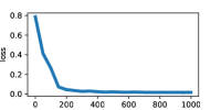
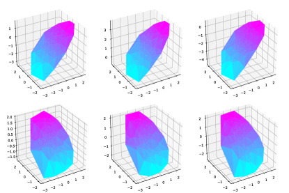
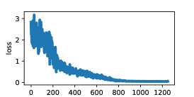
The first test will be a 2D Gaussian that has its mean given by another variable: let $X$ and $Y$ be 2D independent standard Gaussian variables and consider $\mu$ to be the distribution of $X+Y$. The implementation of the DCMQ algorithm is available at (?) and the results are presented in figures 1 and 2. The DCMQ algorithm is shown to converge well (cf. figure 1). Moreover the quantization seems to have desirable properties i.e., it follows the conditional information (the mean). See legend of the figures for additional information.

Figure 1: Conditional quantization with $Q=10$ points for the test in section 3.1. Left image: Convergence of the loss function. Right images : Five points $x_{1},...,x_{5}\in\mathcal{X}=\mathbb{R}^{2}$ are sampled from $\mu^{X}$ (plotted as blue triangles); the DNN (after training) is asked to quantize the conditional distribution $\mu_{x_{b}}$ for each $b\leq 5$ (red stars). Recall that $\mu_{x_{b}}$ is a Gaussian shifted by $x_{b}$. The quantization points follow precisely the indicated mean.

Figure 2: Conditional quantization with $Q=10$ points for the test in section 3.1. The conditional quantization points $x\in\mathbb{R}^{2}\mapsto\mathbf{y}^{dcmq}(x)=(\mathbf{y}_{1}^{dcmq}(x),...,\mathbf{y}_{10}^{dcmq}(x))\in(\mathbb{R}^{2})^{10}$ are plotted as functions of $x$; each column is a dimension of $\mathbf{y}^{dcmq}(x)$ (each row a dimension of the value itself); for graphical convenience we only plot the first $3$ quantized functions i.e. $\mathbf{y}_{1}^{dcmq}(x)$ (first column), $\mathbf{y}_{2}^{dcmq}(x)$ (second column), $\mathbf{y}_{3}^{dcmq}(x)$ (third column). The functions appear smooth and move synchronously, which is a suitable property of the conditional quantization, see section 2.

3.2 Quantization of 2D Gaussian : the multiplicative case

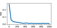
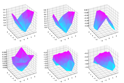
We move now to another test case where the condition enters multiplicatively; with the notations above ($X$ and $Y$ 2D independent standard Gaussian variables) $\mu$ is taken to be the distribution of $X\cdot Y$. The results are presented in figures 3 and 4. The DCMQ algorithms converges well and the quantization follows the conditional information.

Figure 3: Conditional quantization with $Q=10$ points for the test in section 3.2. Left image: Convergence of the loss function. Right images : Five points $x_{1},...,x_{5}\in\mathcal{X}=\mathbb{R}^{2}$ are sampled from $\mu^{X}$(blue triangles); the DNN (after training) is asked to quantize $\mu_{x_{b}}$ for each $b\leq 5$ (red stars). Here $\mu_{x_{b}}$ is a Gaussian multiplied in each direction by $x_{b}$. So, for instance when a point $x_{b}$ has both component values large, the corresponding quantization will look like the quantization of a bi-variate normal. But when $x_{b}$ is close to some axis, the quantization will act on a very elliptical form distribution because one of the Gaussian is multiplied by a small constant. This expected behavior is reproduced well by the converged DNN.

Figure 4: Conditional quantization with $Q=10$ points for the test in section 3.2. We plot the conditional quantization functions $\mathbf{y}_{1}^{dcmq}(x),\mathbf{y}_{2}^{dcmq}(x),\mathbf{y}_{3}^{dcmq}(x)$ as in figure 2.

3.3 Quantization of a 1D Gaussian mixture crossing

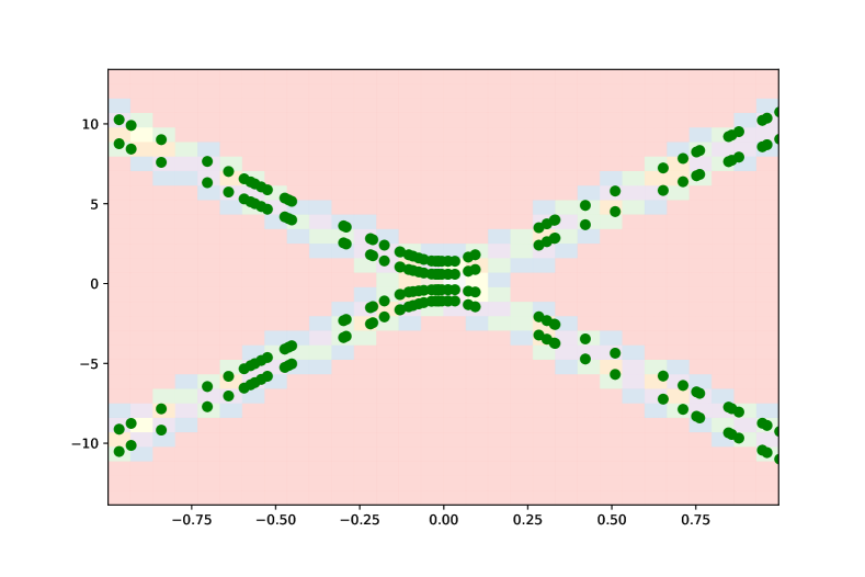
We consider now the situation of a parameter $X$ uniform in $[-1,1]$ and the dependent variable $Y$ will be a even mixture of two 1D Gaussians, centered at $\pm 10X$; the joint density of $(X,Y)$ is plotted in figure 5 (background). The DCMQ algorithm converges well and the quantization follows the expected laws.

Figure 5: Conditional quantization with $Q=4$ points for the test described in section 3.3. Top image: Convergence of the loss function. Bottom image : The joint density of $(X,Y)$ is plotted in background (red are low values, blue are high values). The green dots indicate the quantized values. Note that each of the two parts of the mixture is assigned two quantization points that move along the mean.

4 The Deep Conditional Quantization through joint sampling : MNIST restauration

Conditional sampling from $\mu_{x}$ as in section 3 is not always possible and data presentation can indicate joint sampling as the only way to obtain a couple $(X,Y)$ ; this arrives especially when $X$ is continuous and it is impossible to ensure that $X$ has a desired value $x$. We adapt in this section the previous algorithm and test on a image reconstruction task.

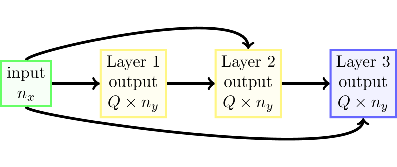
The default neural network architecture is as follows : all layers are fully-connected and have as output a tensor of shape $B\times n_{y}\times Q$ ($B$ is the batch size) ; the first (input) layer takes data of size $B\times n_{x}$. All layers act on the output of the previous layer concatenated with the condition (input of the first layer of shape $B\times n_{x}$). This architecture is akin to a ”constant attention” (?; ?) U-net(?). In our tests the default is to use $3$ such dense layers with ReLU activations. A graphical description is given in figure 6.

Figure 6: Default network architecture used in section 4 (batch size $B=1$).

The algorithm minimizes (by sampling) the following loss functional (with obvious notations)

$$\mathbb{E}_{x\sim\mu^{X}}\left[d\left(\mu_{x},\frac{1}{Q}\sum_{q=1}^{Q}\delta_{x,\mathbf{y}_{q}^{dcmq}(\mu_{x})}\right)^{2}\right].$$ (6)

Algorithm A2 Deep Conditional Measure Quantization algorithm through joint sampling : DCMQ-J

1:procedure DCMQ-J

2:     $\bullet$ set batch size $B$, sampling size $J$, parameters $a$ (default $10^{-6}$), and $r$ (default $1.$), minimization algorithm (default = Adam (?)); max iterations (default $1000$)

3:     $\bullet$ choose a network architecture and initialize layers (default : cf. fig. 6);

4:     while (max iteration not reached) do

5:         $\bullet$ sample i.i.d $(x_{1},y_{1}),...,(x_{B},y_{B})$ from the dataset ;

6:         $\bullet$ propagate $x_{1},...,x_{B}$ through the network to obtain $\mathbf{y}^{dcmq}(x_{b})\in\mathcal{Y}^{Q}$, $b\leq B$ ;

7:         $\bullet$ compute the loss $\mathcal{L}=\frac{1}{B}\sum_{b=1}^{B}d\left(\delta_{x_{b},y_{b}},\frac{\sum_{q=1}^{Q}\delta_{x_{b},\mathbf{y}_{q}^{dcmq}(x_{b})}}{Q}\right)^{2}$ ;

8:         $\bullet$ update the network as specified by the stochastic optimization algorithm (using backpropagation) to minimize the loss $\mathcal{L}$.

9:     end while

10:end procedure

Figure 7: MNIST reconstruction results as described in section 4.

Remark 7.

Note that an alternative formulation can be proposed that employs the following loss functional instead of (6) :

$$d\left(\mu,\frac{1}{Q}\sum_{q=1}^{Q}\delta_{x,\mathbf{y}_{q}^{dcmq}(\mu_{x})}\right)^{2}.$$ (7)

This loss has lower variance (gain of order $O(\frac{1}{B})$) but requires more computations per iteration : $O(B^{2}(1+Q)^{2}n_{y}+B^{2}n_{x})$ instead of $O(BQ^{2}n_{y})$. The sampled version used by the algorithm is in this case : $d\left(\frac{\sum_{b=1}^{B}\delta_{x_{b},y_{b}}}{B},\frac{\sum_{b=1}^{B}\sum_{q=1}^{Q}\delta_{x_{b},\mathbf{y}_{q}^{dcmq}(x_{b})}}{B\cdot Q}\right)^{2}$.

The algorithm was tested on the MNIST dataset for an inpainting (image restoration) task i.e., it was requested to restore the whole image using only a part of it as input ; in all cases we considered a part of the image as known corresponding to the condition i.e., the $X$ component (of dimension $n_{x}$), and another part as unknown, corresponding to the $Y$ component (of dimension $n_{y}$) ; the $Q=1$ quantization was learned using the train dataset and, at test time, we asked the algorithm to output the quantization for images in the test MNIST dataset. Several situations were considered for the unknown part $Y$ depicted in gray in figure 7 (the description is consistent with the order of results there) : right half, left half, upper half, lower half, lower right $2/3\times 2/3$ corner, random pixels covering $90\%$ of all $28\times 28$ pixels. The known part, plotted in the first row, was given as input ; the true images are in the second row and the guess of the algorithm is in the third row. Good agreement is observed in all test situations as the algorithm manages to reconstruct well the missing parts.

5 Concluding remarks

In this paper we discuss the quantization of conditional probability laws. We first prove that in general the quantization can be represented as measurable function and then, in a particular case, we give a theoretical result that ensures the quantization points depend continuously on the condition. Then, a deep learning algorithm is introduced using Huber-energy kernels to find numerically the solution of the quantization problem. The procedure is tested on some standard cases and shows promising results.

References

- Agiomyrgiannakis and Stylianou 2007 Agiomyrgiannakis, Y., and Stylianou, Y. 2007. Conditional Vector Quantization for Speech Coding. IEEE Transactions on Audio, Speech, and Language Processing 15(2):377–386. Conference Name: IEEE Transactions on Audio, Speech, and Language Processing.
- Bahdanau, Cho, and Bengio 2014 Bahdanau, D.; Cho, K.; and Bengio, Y. 2014. Neural machine translation by jointly learning to align and translate.
- Bavarian et al. 2022 Bavarian, M.; Jun, H.; Tezak, N.; Schulman, J.; McLeavey, C.; Tworek, J.; and Chen, M. 2022. Efficient Training of Language Models to Fill in the Middle. arXiv:2207.14255 [cs].
- Berlinet, Cadre, and Gannoun 2001a Berlinet, A.; Cadre, B.; and Gannoun, A. 2001a. Estimation of conditional L1-median from dependent observations. Statistics & Probability Letters 55(4):353–358.
- Berlinet, Cadre, and Gannoun 2001b Berlinet, A.; Cadre, B.; and Gannoun, A. 2001b. On The Conditional L 1-median and its estimation. Journal of Nonparametric Statistics 13(5):631–645. Publisher: Taylor & Francis.
- Bishop 1994 Bishop, C. M. 1994. Mixture density networks. Technical Report, Aston University.
- Brown and Purves 1973 Brown, L. D., and Purves, R. 1973. Measurable Selections of Extrema. The Annals of Statistics 1(5):902–912. Publisher: Institute of Mathematical Statistics.
- Brown et al. 2020 Brown, T. B.; Mann, B.; Ryder, N.; Subbiah, M.; Kaplan, J.; Dhariwal, P.; Neelakantan, A.; Shyam, P.; Sastry, G.; Askell, A.; Agarwal, S.; Herbert-Voss, A.; Krueger, G.; Henighan, T.; Child, R.; Ramesh, A.; Ziegler, D. M.; Wu, J.; Winter, C.; Hesse, C.; Chen, M.; Sigler, E.; Litwin, M.; Gray, S.; Chess, B.; Clark, J.; Berner, C.; McCandlish, S.; Radford, A.; Sutskever, I.; and Amodei, D. 2020. Language models are few-shot learners.
- Cascales, Kadets, and Rodríguez 2010 Cascales, B.; Kadets, V.; and Rodríguez, J. 2010. Measurability and selections of multi-functions in Banach spaces. Journal of Convex Analysis 17(1):229–240.
- Chatalic et al. 2022 Chatalic, A.; Schreuder, N.; Rosasco, L.; and Rudi, A. 2022. Nyström Kernel Mean Embeddings. In Chaudhuri, K.; Jegelka, S.; Song, L.; Szepesvari, C.; Niu, G.; and Sabato, S., eds., Proceedings of the 39th International Conference on Machine Learning, volume 162 of Proceedings of Machine Learning Research, 3006–3024. PMLR.
- Chazal, Levrard, and Royer 2021 Chazal, F.; Levrard, C.; and Royer, M. 2021. Optimal quantization of the mean measure and applications to statistical learning.
- Constantinides and Lim 1984 Constantinides, A., and Lim, J. 1984. Quantization noise in data conversion systems. IEEE Transactions on Communications 32(10):1218–1225.
- Crochiere and Rabiner 1989 Crochiere, R., and Rabiner, L. 1989. Multirate digital signal processing. Proceedings of the IEEE 77(4):463–481.
- et al. 2020 et al., T. B. 2020. Language models are few-shot learners. In Larochelle, H.; Ranzato, M.; Hadsell, R.; Balcan, M.; and Lin, H., eds., Advances in Neural Information Processing Systems, volume 33, 1877–1901. Curran Associates, Inc.
- Gannoun, Saracco, and Yu 2003 Gannoun, A.; Saracco, J.; and Yu, K. 2003. Nonparametric prediction by conditional median and quantiles. Journal of statistical Planning and inference 117(2):207–223.
- Graf and Luschgy 2007 Graf, S., and Luschgy, H. 2007. Foundations of quantization for probability distributions. Springer.
- Graham 1972 Graham, R. 1972. An efficient algorithm for determining the convex hull of a finite planar set. Information Processing Letters 1(4):132–133.
- Kingma and Ba 2017 Kingma, D. P., and Ba, J. 2017. Adam: A Method for Stochastic Optimization. arXiv:1412.6980 [cs].
- Kreitmeier 2011 Kreitmeier, W. 2011. Optimal vector quantization in terms of Wasserstein distance. Journal of Multivariate Analysis 102(8):1225–1239.
- Kuratowski and Ryll-Nardzewski 1965 Kuratowski, K., and Ryll-Nardzewski, C. 1965. A general theorem on selectors. Bulletin de l’Académie Polonaise des Sciences, Série des Sciences Mathématiques, Astronomiques et Physiques 13:397–403.
- Lyons 1995 Lyons, T. J. 1995. Cubature on Wiener space. Journal of Functional Analysis 129(2):483–509.
- Mehra, Rao, and Upadrasta 1991 Mehra, K.; Rao, M. S.; and Upadrasta, S. 1991. A smooth conditional quantile estimator and related applications of conditional empirical processes. Journal of Multivariate Analysis 37(2):151–179.
- OpenAI 2022 OpenAI. 2022. ChatGPT: Optimizing Language Models for Dialogue. https://openai.com/blog/chatgpt/, at 2023-01-16.
- Pages 2015 Pages, G. 2015. Cubature formulae and gaussian quadrature rules. Journal of Complexity 31:1–29.
- Pagès 2018 Pagès, G. 2018. Optimal Quantization Methods I: Cubatures. In Pagès, G., ed., Numerical Probability: An Introduction with Applications to Finance. Cham: Springer International Publishing. 133–173.
- Parks and Burrus 1985 Parks, T., and Burrus, C. 1985. Chebyshev-hermite and chebyshev-legendre orthonormal expansions of signals. IEEE Transactions on Circuits and Systems CAS-32(8):851–856.
- Proakis 1995 Proakis, J. G. 1995. Digital Communications. McGraw-Hill New York.
- Sculley and Hinton 2010 Sculley, D., and Hinton, G. 2010. Web-scale k-means clustering. In Proceedings of the 19th international conference on World wide web, 1177–1178. ACM.
- Shelhamer, Long, and Darrell 2017 Shelhamer, E.; Long, J.; and Darrell, T. 2017. Fully Convolutional Networks for Semantic Segmentation. IEEE Transactions on Pattern Analysis and Machine Intelligence 39(4):640–651. arxiv:1411.4038.
- Sriperumbudur et al. 2010 Sriperumbudur, B. K.; Gretton, A.; Fukumizu, K.; Schölkopf, B.; and Lanckriet, G. R. 2010. Hilbert space embeddings and metrics on probability measures. The Journal of Machine Learning Research 11:1517–1561.
- Strauss and Oliva 2021 Strauss, R. R., and Oliva, J. B. 2021. Arbitrary conditional distributions with energy.
- Suefusa et al. 2020 Suefusa, K.; Nishida, T.; Purohit, H.; Tanabe, R.; Endo, T.; and Kawaguchi, Y. 2020. Anomalous Sound Detection Based on Interpolation Deep Neural Network. In ICASSP 2020 - 2020 IEEE International Conference on Acoustics, Speech and Signal Processing (ICASSP), 271–275.
- Szekely, Rizzo, and others 2005 Szekely, G. J.; Rizzo, M. L.; et al. 2005. Hierarchical clustering via joint between-within distances: Extending ward’s minimum variance method. Journal of classification 22(2):151–184.
- Székely and Rizzo 2013 Székely, G. J., and Rizzo, M. L. 2013. Energy statistics: A class of statistics based on distances. Journal of Statistical Planning and Inference 143(8):1249–1272.
- Turinici 2022 Turinici, G. 2022. Huber-energy measure quantization. Arxiv : 2212.08162.
- Turinici 2023 Turinici, G. 2023. Huber energy measure quantization repository. GitHub repository https://github.com/gabriel-turinici/Huber-energy-measure-quantization.
- Vaidyanathan 1993 Vaidyanathan, P. P. 1993. Multirate systems and filterbanks. Prentice Hall Englewood Cliffs, NJ.
- Vaswani et al. 2017 Vaswani, A.; Shazeer, N.; Parmar, N.; Uszkoreit, J.; Jones, L.; Gomez, A. N.; Kaiser, L.; and Polosukhin, I. 2017. Attention Is All You Need.
- Vuong et al. 2023 Vuong, T.-L.; Le, T.; Zhao, H.; Zheng, C.; Harandi, M.; Cai, J.; and Phung, D. 2023. Vector Quantized Wasserstein Auto-Encoder.
- Wang et al. 2019 Wang, X.; Yu, K.; Dong, C.; Tang, X.; and Loy, C. C. 2019. Deep network interpolation for continuous imagery effect transition. In Proceedings of the IEEE/CVF Conference on Computer Vision and Pattern Recognition (CVPR).
- White 1992 White, H. 1992. Nonparametric Estimation of Conditional Quantiles Using Neural Networks. In Page, C., and LePage, R., eds., Computing Science and Statistics, 190–199. New York, NY: Springer New York.
- Zhou and Ooka 2020 Zhou, Q., and Ooka, R. 2020. Comparison of different deep neural network architectures for isothermal indoor airflow prediction. In Building Simulation, volume 13(6), 1409–1423. Springer.
- Zhou et al. 2021 Zhou, X.; Jiao, Y.; Liu, J.; and Huang, J. 2021. A Deep Generative Approach to Conditional Sampling.