Power Utility Maximization with Expert Opinions at Fixed Arrival Times in a Market with Hidden Gaussian Drift

Abstract

In this paper we study optimal trading strategies in a financial market in which stock returns depend on a hidden Gaussian mean reverting drift process. Investors obtain information on that drift by observing stock returns. Moreover, expert opinions in the form of signals about the current state of the drift arriving at fixed and known dates are included in the analysis. Drift estimates are based on Kalman filter techniques. They are used to transform a power utility maximization problem under partial information into an optimization problem under full information where the state variable is the filter of the drift. The dynamic programming equation for this problem is studied and closed-form solutions for the value function and the optimal trading strategy of an investor are derived. They allow to quantify the monetary value of information delivered by the expert opinions. We illustrate our theoretical findings by results of extensive numerical experiments.

MSC Classification]91G10 93E20 93E11 60G35

1 Introduction

In dynamic portfolio selection problems optimal trading strategies depend crucially on the drift of the underlying asset return processes. That drift describes the expected asset returns, varies over time and is driven by certain stochastic factors such as dividend yields, the firm’s return on equity, interest rates and macroeconomic indicators. This was already addressed in the seminal paper of Merton (Merton (1971), , Sec. 9). We also refer to other early articles by Bielecki and Pliska Bielecki_Pilska (1999) , Brennan, Schwartz, Lagnado Brennan et al (1997) and Xia Xia (2001) . The dependence of the drift process on these factors is usually not perfectly known and some of the factors may be not directly observable. Therefore, it is reasonable to model the drift as an unobservable stochastic process for which only statistical estimates are available. Then solving the associated portfolio problems has to be based on such estimates of the drift process.

For the one-period Markowitz model the surprisingly large impact of statistical errors in the estimation of model parameters on mean-variance optimal portfolios is often reported in the literature, e.g. by Broadie Broadie (1993) . Estimating the drift with a reasonable degree of precision based only on historical asset prices is known to be almost impossible. This is nicely shown in Rogers (Rogers (2013), , Chapter 4.2) for a model in which the drift is even constant. For a reliable estimate extremely long time series of data are required which are usually not available. Further, assuming a constant drift over longer periods of time is quite unrealistic. Drifts tend to fluctuate randomly over time and drift effects are often overshadowed by volatility.

For these reasons, portfolio managers and traders try to diversify their observation sources and also rely on external sources of information such as news, company reports, ratings and benchmark values. Further, they increasingly turn to data outside of the traditional sources that companies and financial markets provide. Examples are social media posts, internet search, satellite imagery, sentiment indices, pandemic data, product review trends and are often related to Big Data analytics. Finally, they use views of financial analysts or just their own intuitive views on the future asset performance.

In the literature these outside sources of information are coined expert opinions or more generally alternative data, see Chen and Wong Chen Wong (2022) , Davis and Lleo Davis and Lleo (2022) . In this paper we will use the first term. After an appropriate mathematical modeling as additional noisy observations they are included in the drift estimation and the construction of optimal portfolio strategies. That approach goes back to the celebrated Black-Litterman model which is an extension of the classical one-period Markowitz model, see Black and Litterman Black_Litterman (1992) . The idea is to improve return predictions using expert opinions by means of a Bayesian updating of the drift estimate.

Instead of a static one-period model we consider in this paper a continuous-time model for asset prices. Additional information in the form of expert opinions arrive repeatedly over time. Davis and Lleo Davis and Lleo (2013_1) coined this approach “Black–Litterman in Continuous Time” (BLCT). More precisely, we study a hidden Gaussian model where asset returns are driven by an unobservable mean-reverting Gaussian process. Information on the drift is of mixed type. First investors observe stock prices or equivalently the return process. Moreover, investors may have access to expert opinions arriving at already known discrete time points in a form of unbiased drift estimates. Since the investors’ ability to construct good trading strategies depends on the quality of the hidden drift estimation we study a filtering problem. There the aim is to find the conditional distribution of the drift given the available information drawn from the return observations and expert opinions.

For investors who observe only the return process that filter known as the classical Kalman–Bucy filter, see for example Liptser and Shiryaev Liptser-Shiryaev . Based on this one can derive the filter for investors who also observe expert opinions by a Bayesian update of the current drift estimate at each information date. This constitutes the above mentioned continuous-time version of the static Black–Litterman approach.

Utility maximization problems for partially informed investors have been intensively studied in the last years. For models with Gaussian drift we refer to to Lakner Lakner (1998) and Brendle Brendle2006 . Results for models in which the drift is described by a continuous-time hidden Markov chain are given in Rieder and Bäuerle Rieder_Baeuerle2005 , Sass and Haussmann Sass and Haussmann (2004) and more recently by Chen and Wong Chen Wong (2022) . A good overview with further references and generalization can be found in Björk et al. Bjoerk et al (2010) .

For the literature on BLCT in which expert opinions are included we refer to a series of papers Gabih et al (2014) ; Gabih et al (2019) FullInfo ; Sass et al (2017) ; Sass et al (2021) ; Sass et al (2022) of the present authors and of Sass and Westphal. They investigate utility maximization problems for investors with logarithmic preferences in market models with a hidden Gaussian drift process and discrete-time expert opinions. The case of continuous-time expert opinions and power utility maximization is treated in a series of papers by Davis and Lleo, see Davis and Lleo (2013_1) ; Davis and Lleo (2020) ; Davis and Lleo (2022) and the references therein. Power utility maximization problems for drift processes described by continuous-time hidden Markov chains have been studied in Frey et al. Frey et al. (2012) ; Frey-Wunderlich-2014 . Finally, we refer to our companion paper Gabih et al (2022) Nirvana where we investigate the well posedness of power utility maximization problems which are addressed in the present paper.

In the present paper we study in detail the case of power utility maximization for market models with a hidden Gaussian drift. While for continuous-time expert opinions results are available from the work of Davis and Lleo, see Davis and Lleo (2013_1) ; Davis and Lleo (2020) ; Davis and Lleo (2022) , the case of discrete-time expert opinions was only considered in the PhD of Kondakji Kondkaji (2019) on which this paper is based. Recently, a few results of Kondkaji (2019) were briefly mentioned in Sass et al. Sass et al (2022) and applied in numerical experiments. Our main results are presented in Theorems 6.1 and 6.3 where we derive a backward recursion for the value function and the optimal strategy of the partially informed investors observing also discrete-time expert opinions. Further, in Sec. 7 we present results of extensive numerical experiments. There we study in particular the asymptotic properties of filters, value functions and optimal strategies for high-frequency experts and the monetary value of expert opinions.

The paper is organized as follows. In Sec. 2 we introduce the model for our financial market including the expert opinions and define information regimes for investors with different sources of information. Further, we formulate the portfolio optimization problem. Sec. 3 states for the different information regimes the filter equations for the corresponding conditional mean and conditional covariance process. Then it reviews properties of the filter, in particular the asymptotic filter behavior for high-frequency expert opinions. Sec. 4 is devoted to the solution of the power utility maximization problem. That problem is reformulated as an equivalent stochastic optimal control problem which can be solved by dynamic programming techniques. Solutions are presented for the fully informed investor. Sec. 5 presents the solution for partially informed investors combining return observations with diffusion type expert opinions and Sec. 6 studies the case of investors observing discrete-time experts. Sec. 7 illustrates the theoretical findings by numerical results.

Notation

Throughout this paper, we use the notation $I_{d}$ for the identity matrix in $\mathbb{R}^{d\times d}$, $0_{d}$ denotes the null vector in $\mathbb{R}^{d}$, $0_{d\times m}$ the null matrix in $\mathbb{R}^{d\times m}$. For a symmetric and positive-semidefinite matrix $A\in\mathbb{R}^{d\times d}$ we call a symmetric and positive-semidefinite matrix $B\in\mathbb{R}^{d\times d}$ the square root of $A$ if $B^{2}=A$. The square root is unique and will be denoted by $A^{1/2}$. For a vector $X$ we denote by $\left\lVert X\right\rVert$ the Euclidean norm. Unless stated otherwise, whenever $A$ is a matrix, $\lVert A\rVert$ denotes the spectral norm of $A$.

2 Financial Market and Optimization Problem

2.1 Price Dynamics

We model a financial market with one risk-free and multiple risky assets. The setting is based on Gabih et al. Gabih et al (2014) ; Gabih et al (2019) FullInfo and Sass et al. Sass et al (2017) ; Sass et al (2022) ; Sass et al (2021) . For a fixed date $T>0$ representing the investment horizon, we work on a filtered probability space $(\Omega,\pazocal{G},\mathbb{G},\mathbb{P})$, with filtration $\mathbb{G}=(\pazocal{G}_{t})_{t\in[0,T]}$ satisfying the usual conditions. All processes are assumed to be $\mathbb{G}$-adapted.

We consider a market model for one risk-free bond with constant price $S^{0}_{t}=1$ and $d$ risky securities whose return process $R=(R^{1},\ldots,R^{d})$ is defined by

$$dR_{t}=\mu_{t}\,dt+\sigma_{R}\,dW^{R}_{t},$$ (1)

for a given $d_{1}$-dimensional $\mathbb{G}$-adapted Brownian motion $W^{R}$ with $d_{1}\geq d$. The volatility matrix $\sigma_{R}\in\mathbb{R}^{d\times d_{1}}$ is assumed to be constant over time such that $\Sigma_{R}:=\sigma_{R}\sigma_{R}^{\top}$ is positive definite. In this setting the price process $S=(S^{1},\ldots,S^{d})$ of the risky securities reads as

$$dS_{t} =diag(S_{t})\,dR_{t},~{}~{}S_{0}=s_{0},$$ (2)

with some fixed initial value $s_{0}=(s_{0}^{1},\ldots,s_{0}^{d})$. Note that for the solution to the above SDE it holds

$$\log S_{t}^{i}-\log s_{0}^{i} =\int\limits_{0}^{t}\mu_{s}^{i}ds+\sum\limits_{j=1}^{d_{1}}\Big{(}\sigma_{R}^{ij}W_{t}^{R,j}-\frac{1}{2}(\sigma_{R}^{ij})^{2}t\Big{)}=R_{t}^{i}-\frac{1}{2}\sum\limits_{j=1}^{d_{1}}(\sigma_{R}^{ij})^{2}t,\quad i=1,\ldots,d.$$

So we have the equality $\mathbb{G}^{R}=\mathbb{G}^{\log S}=\mathbb{G}^{S}$, where for a generic process $X$ we denote by $\mathbb{G}^{X}$ the filtration generated by $X$. This is useful since it allows to work with $R$ instead of $S$ in the filtering part.

The dynamics of the drift process $\mu=(\mu_{t})_{t\in[0,T]}$ in (1) are given by the stochastic differential equation (SDE)

$$d\mu_{t}=\kappa(\overline{\mu}-\mu_{t})\,dt+\sigma_{\mu}\,dW^{\mu}_{t},$$ (3)

where $\kappa\in\mathbb{R}^{d\times d}$, $\sigma_{\mu}\in\mathbb{R}^{d\times d_{2}}$ and $\overline{\mu}\in\mathbb{R}^{d}$ are constants such that the matrices $\kappa$ and $\Sigma_{\mu}:=\sigma_{\mu}\sigma_{\mu}^{\top}$ are positive definite, and $W^{\mu}$ is a $d_{2}$-dimensional Brownian motion such that $d_{2}\geq d$. For the sake of simplification and shorter notation we assume that the Wiener processes $W^{R}$ and $W^{\mu}$ driving the return and drift process, respectively, are independent. We refer to Brendle Brendle2006 , Colaneri et al. Colaneri et al (2021) and Fouque et al. Fouque et al. (2015) for the general case. Here, $\overline{\mu}$ is the mean-reversion level, $\kappa$ the mean-reversion speed and $\sigma_{\mu}$ describes the volatility of $\mu$. The initial value $\mu_{0}$ is assumed to be a normally distributed random variable independent of $W^{\mu}$ and $W^{R}$ with mean $\overline{m}_{0}\in\mathbb{R}^{d}$ and covariance matrix $\overline{q}_{0}\in\mathbb{R}^{d\times d}$ assumed to be symmetric and positive semi-definite. It is well-known that the solution to SDE (3) is known as Ornstein-Uhlenbeck process which is a Gaussian process given by

$$\mu_{t} =\overline{\mu}+e^{-\kappa t}\Big{[}(\mu_{0}-\overline{\mu})+\int_{0}^{t}e^{\kappa s}\sigma_{\mu}dW^{\mu}_{s}\Big{]},\quad t\geq 0.$$ (4)

2.2 Expert Opinions

We assume that investors observe the return process $R$ but they neither observe the factor process $\mu$ nor the Brownian motion $W^{R}$. They do however know the model parameters such as $\sigma_{R},\kappa,\overline{\mu},\sigma_{\mu}$ and the distribution $\pazocal{N}(\overline{m}_{0},\overline{q}_{0})$ of the initial value $\mu_{0}$. Information about the drift $\mu$ can be drawn from observing the returns $R$. A special feature of our model is that investors may also have access to additional information about the drift in form of expert opinions such as news, company reports, ratings or their own intuitive views on the future asset performance. The expert opinions provide noisy signals about the current state of the drift arriving at known deterministic time points $0=t_{0}<t_{1}<\ldots<t_{N-1}<T$. For the sake of convenience we also write $t_{N}=T$ although no expert opinion arrives at time $t_{N}$. The signals or “the expert views” at time $t_{k}$ are modelled by $\mathbb{R}^{d}$-valued Gaussian random vectors $Z_{k}=(Z_{k}^{1},\ldots,Z_{k}^{d})^{\top}$ with

$$Z_{k}=\mu_{t_{k}}+{\Gamma}^{\frac{1}{2}}\varepsilon_{k},\quad k=0,\ldots,n-1,$$ (5)

where the matrix $\Gamma\in\mathbb{R}^{d\times d}$ is symmetric and positive definite. Further, $(\varepsilon_{k})_{k=0,...,n-1}$ is a sequence of independent standard normally distributed random vectors, i.e., $\varepsilon_{k}\sim~{}\pazocal{N}(0,I_{d})$. It is also independent of both the Brownian motions $W^{R},W^{\mu}$ and the initial value $\mu_{0}$ of the drift process. That means that, given $\mu_{t_{k}}$, the expert opinion $Z_{k}$ is $\pazocal{N}(\mu_{t_{k}},\Gamma)$-distributed. So, $Z_{k}$ can be considered as an unbiased estimate of the unknown state of the drift at time $t_{k}$. The matrix $\Gamma$ is a measure of the expert’s reliability. In a model with $d=1$ risky asset $\Gamma$ is just the variance of the expert’s estimate of the drift at time $t_{k}$: the larger $\Gamma$ the less reliable is the expert.

Modeling expert opinions as normally distributed random variables corresponds well to a variety of additional information on average stock returns available in real-world markets. We refer to Davis and Lleo Davis and Lleo (2020) for more details about an appropriate preprocessing, debiasing and approximation of such extra information by Gaussian models. Let us briefly sketch the mathematical modeling of analyst views in terms of confidence intervals. Inspired by Davis and Lleo (2020) we consider the following example of a view at time $t=t_{k}$: “My research leads me to believe that the average stock return lies within a range of $6\%$ to $10\%$, and I’m $90\%$ confident about this”. This view can be treated as a $90\%$-confidence interval for the unknown mean $\mu_{t_{k}}$ of a Gaussian distribution centered at $0.08$, which is the observed $Z_{k}$. The corresponding variance $\Gamma_{k}$ is chosen such that the boundaries of the interval are $0.06$ and $0.10$. We also want to emphasize that the Gaussian expert opinions allow to work with Kalman filtering techniques. For other distributions, in general no closed-form filters are available.

The above model of discrete-time expert opinions can be modified such that expert opinions arrive not at fixed and known dates but at random times $(T_{k})_{k\in\mathbb{N}}$. That approach together with results for filtering and maximization of log-utility was studied in detail in Sass et al. Sass et al (2021) . There the arrival times are modeled as the jump times of a Poisson process. The maximization of power utility was considered in Kondkaji (2019) and will be addressed in a forthcoming paper.

One may also allow for relative expert views where experts give an estimate for the difference in the drift of two stocks instead of absolute views. This extension can be studied in Schöttle et al. Schoettle et al. (2010) where the authors show how to switch between these two models for expert opinions by means of a pick matrix.

In addition to expert opinions arriving at discrete time points we will also consider expert opinions arriving continuously over time as in Davis and Lleo Davis and Lleo (2013_1) ; Davis and Lleo (2020) who called this approach “Black–Litterman in Continuous Time”. This is motivated by the results of Sass et al. Sass et al (2021) ; Sass et al (2022) who show that asymptotically as the arrival frequency tends to infinity and the expert’s variance $\Gamma$ grows linearly in that frequency the information drawn from these expert opinions is essentially the same as the information one gets from observing yet another diffusion process. This diffusion process can then be interpreted as an expert who gives a continuous-time estimation about the current state of the drift. Another interpretation is that the diffusion process models returns of assets which are not traded in the portfolio but depend on the same stochastic factors and are observable by the investor. Let these continuous-time expert opinions be given by the diffusion process

$$dJ_{t}=\mu_{t}dt+\sigma_{J}dW_{t}^{J}$$ (6)

where $W_{t}^{J}$ is a $d_{3}$-dimensional Brownian motion independent of $W_{t}^{R}$ and $W^{\mu}$ and such that with $d_{3}\geq d$. The volatility matrix $\sigma_{J}\in\mathbb{R}^{d\times d_{3}}$ is assumed to be constant over time such that the matrix $\Sigma_{J}:=\sigma_{J}\sigma_{J}^{\top}$ is positive definite. In Subsecs. 4.1 and 7.4 we show that based on this model and on the diffusion approximations provided in Sass et al (2022) one can find efficient approximative solutions to utility maximization problems for partially informed investors observing high-frequency discrete-time expert opinions.

2.3 Investor Filtration

We consider various types of investors with different levels of information. The information available to an investor is described by the investor filtration $\mathbb{F}^{H}=(\pazocal{F}^{H}_{t})_{t\in[0,T]}$. Here, $H$ denotes the information regime for which we consider the cases $H=R,Z,J,F$ and the investor with filtration $\mathbb{F}^{H}=(\pazocal{F}^{H}_{t})_{t\in[0,T]}$ is called the $H$-investor. The $R$-investor observes only the return process $R$, the $Z$-investor combines return observations with the discrete-time expert opinions $Z_{k}$ while the $J$-investor observes the return process together with the continuous-time expert $J$. Finally, the $F$-investor has full information and can observe the drift process $\mu$ directly and of course the return process. For stochastic drift this case is not realistic, but we use it as a benchmark. It will serve as a limiting case for high-frequency expert opinions with fixed covariance matrix $\Gamma$, see Subsec. 3.3, Thm. 3.9.

The $\sigma$-algebras $\pazocal{F}^{H}_{t}$ representing the $H$-investor’s information at time $t\in[0,T]$ are defined at initial time $t=0$ by $\pazocal{F}^{F}_{0}=\sigma\{\mu_{0}\}$ for the fully informed investor and by $\pazocal{F}^{H}_{0}=\pazocal{F}^{I}_{0}\subset\pazocal F_{0}^{F}$ for $H=R,Z,J$, i.e., for the partially informed investors. Here, $\pazocal{F}_{0}^{I}$ denotes the $\sigma$-algebra representing a priori information about the initial drift $\mu_{0}$. More details on $\pazocal{F}_{0}^{I}$ are given below. For $t\in(0,T]$ we define

$$\begin{array}[]{rl}\pazocal{F}_{t}^{R}&=\sigma(R_{s},~{}s\leq t)\vee\pazocal{F}_{0}^{I},\\[2.15277pt] \pazocal{F}_{t}^{Z}&=\sigma(R_{s},s\leq t,\,~{}(t_{k},Z_{k}),~{}t_{k}\leq t)\vee\pazocal{F}_{0}^{I},\\[2.15277pt] \pazocal{F}_{t}^{J}&=\sigma(R_{s},J_{s},~{}s\leq t)\vee\pazocal{F}_{0}^{I},\\[2.15277pt] \pazocal{F}_{t}^{F}&=\sigma(R_{s},\mu_{s},~{}s\leq t).\end{array}$$

We assume that the above $\sigma$-algebras $\pazocal{F}_{t}^{H}$ are augmented by the null sets of $\mathbb{P}$.

Note that all partially informed investors ($H=R,J,Z$) start at $t=0$ with the same initial information given by $\pazocal{F}_{0}^{I}$. The latter models prior knowledge about the drift process at time $t=0$, e.g., from observing returns or expert opinions in the past, before the trading period $[0,T]$. The expert opinion $Z_{0}$ arriving at time $t=0$ does not belong to this prior information and is therefore excluded from $\pazocal{F}_{0}^{Z}$ and only contained in $\pazocal{F}_{t}^{Z}$ for $t>0$. At first glance this may appear not consistent but it will facilitate below in Subsec. 2.6 the formal definition of the monetary value of the expert opinions.

We assume that the conditional distribution of the initial value drift $\mu_{0}$ given $\pazocal{F}_{0}^{I}$ is the normal distribution $\pazocal{N}(m_{0},q_{0})$ with mean $m_{0}\in\mathbb{R}^{d}$ and covariance matrix $q_{0}\in\mathbb{R}^{d\times d}$ assumed to be symmetric and positive semi-definite. In this setting typical examples are:

1. The investor has no information about the initial value of the drift $\mu_{0}$. However, he knows the model parameters, in particular the distribution $\pazocal{N}(\overline{m}_{0},\overline{q}_{0})$ of $\mu_{0}$ with given parameters $\overline{m}_{0}$ and $\overline{q}_{0}$. This corresponds to $\pazocal{F}_{0}^{I}=\{\varnothing,\Omega\}$ and $m_{0}=\overline{m}_{0}$, $q_{0}=\overline{q}_{0}$.

2. The investor can fully observe the initial value of the drift $\mu_{0}$, which corresponds to $\pazocal{F}_{0}^{I}=\pazocal{F}_{0}^{F}=\sigma\{\mu_{0}\}$ and $m_{0}=\mu_{0}(\omega)$ and $q_{0}=0$.

3. Between the above limiting cases we consider an investor who has some prior but no complete information about $\mu_{0}$ leading to $\{\varnothing,\Omega\}\subset\pazocal{F}_{0}^{I}\subset\pazocal F_{0}^{F}$.

2.4 Portfolio and Optimization Problem

We describe the self-financing trading of an investor by the initial capital $x_{0}>0$ and the $\mathbb{F}^{H}$-adapted trading strategy $\pi=(\pi_{t})_{t\in[0,T]}$ where $\pi_{t}\in\mathbb{R}^{d}$. Here $\pi_{t}^{i}$ represents the proportion of wealth invested in the $i$-th stock at time $t$. The assumption that $\pi$ is $\mathbb{F}^{H}$-adapted models that investment decisions have to be based on information available to the $H$-investor which he obtains from from observing assets prices ($H=R$) combined with expert opinions ($H=Z,J$) or with the drift process ($H=F$). Following the strategy $\pi$ the investor generates a wealth process $(X_{t}^{\pi})_{t\in[0,T]}$ whose dynamics reads as

$$\frac{dX_{t}^{\pi}}{X_{t}^{\pi}}=\pi_{t}^{\top}dR_{t} = \pi_{t}^{\top}\mu_{t}\;dt+\pi_{t}^{\top}\sigma_{R}\;dW_{t}^{R},\quad X_{0}^{\pi}=x_{0}.$$ (7)

We denote by

$$\pazocal{A}_{0}^{H}=\Big{\{}\pi=(\pi_{t})_{t}\colon\pi_{t}\in\mathbb{R}^{d},\text{ $\pi$ is $\mathbb{F}^{H}$-adapted },X^{\pi}_{t}>0,{\mathbb{E}}\Big{[}\int\nolimits_{0}^{T}\|\pi_{t}\|^{2}\,dt\Big{]}<\infty\Big{\}}$$ (8)

the class of admissible trading strategies. We assume that the investor wants to maximize the expected utility of terminal wealth for a given utility function $U:\mathbb{R}_{+}\rightarrow\mathbb{R}$ modelling the risk aversion of the investor. In our approach we will use the function

$$\pazocal U_{\theta}(x):=\frac{x^{\theta}}{\theta},\quad\theta\in(-\infty,0)\cup(0,1).$$ (9)

The limiting case for $\theta\rightarrow 0$ for the power utility function leads to the logarithmic utility $\pazocal U_{0}(x):=\ln x$, since we have $\pazocal U_{\theta}(x)-\frac{1}{\theta}=\frac{x^{\theta}-1}{\theta}\xrightarrow[~{}\theta\rightarrow 0~{}]{\text{}}\log x.$ The optimization problem thus reads as

$$\pazocal V_{0}^{H}(x_{0}):=\sup\limits_{\pi\in\pazocal{A}_{0}^{H}}\pazocal D_{0}^{H}(x_{0}\mathchar 24635\relax\;\pi)\quad\text{where}\quad\pazocal D_{0}^{H}(x_{0}\mathchar 24635\relax\;\pi)={\mathbb{E}}\left[\pazocal U_{\theta}(X_{T}^{\pi})\mid\pazocal{F}^{H}_{0}\right],~{}\pi\in\pazocal A^{H}_{0},$$ (10)

where we call $\pazocal D_{0}^{H}(x_{0}\mathchar 24635\relax\;\pi)$ reward function or performance criterion of the strategy $\pi$ and $\pazocal V_{0}^{H}(x_{0})$ value function to given initial capital $x_{0}$. This is for $H\neq F$ a maximization problem under partial information since we have required that the strategy $\pi$ is adapted to the investor filtration $\mathbb{F}^{H}$ while the drift coefficient of the wealth equation (7) is not $\mathbb{F}^{H}$-adapted, it depends on the non-observable drift $\mu$. Note that for $x_{0}>0$ the solution of the SDE (7) is strictly positive. This guarantees that $X_{T}^{\pi}$ is in the domain of logarithmic and power utility.

2.5 Well Posedness of the Optimization Problem

The analysis of the utility maximization problem (10) requires conditions under which the problem is well posed. Problem (10) is said to be well-posed for the $H$-investor, if there exists a constant $C_{\pazocal V}^{H}<\infty$ such that $\pazocal V_{0}^{H}(x_{0})\leq C_{\pazocal V}^{H}$. Then the maximum expected utility of terminal wealth cannot explode in finite time as it is the case for so-called nirvana strategies described e.g. in Kim and Omberg Kim and Omberg (1996) and Angoshtari Angoshtari2013 . Nirvana strategies generate in finite time a terminal wealth with a distribution leading to infinite expected utility although the realizations of terminal wealth may be finite.

In general, well posedness will depend not only on the initial capital $x_{0}$ but on the complete set of model parameters which are $T,\theta,d,\sigma_{R},\sigma_{\mu},\kappa,\overline{\mu},x_{0},\overline{m}_{0},\overline{q}_{0},m_{0},q_{0},\Gamma,n,\sigma_{J}$.

For the power utility function with parameter $\theta<0$ we have $\pazocal U_{\theta}(x)<0$ for all $x>0$. Hence, in that case we can simply choose $C_{\pazocal V}^{H}=0$ and the optimization problem is well-posed for all model parameters with negative $\theta$. The logarithmic utility function ($\theta=0$) is no longer bounded from above but we show below in Subsec. 4.1 that the value function $\pazocal V_{0}^{H}(x_{0})$ is bounded from above by some positive constant $C_{\pazocal V}^{H}$ for any selection of the remaining model parameters. More delicate is the case of power utility with positive parameter $\theta\in(0,1)$ which is also not bounded from above. That case is investigated in detail in our paper Gabih et al (2022) Nirvana where we find conditions on the model parameters ensuring well posedness. One of the findings is that depending on the chosen parameters well-posedness can be guaranteed only if the trading horizon $T$ is smaller than some certain “explosion time”. In the following we always assume that (10) constitutes a well-posed optimization problem.

2.6 Monetary Value of Information

Utility functions and the derived value function to the utility maximization problems (10) do not carry a meaningful unit and therefore it is difficult to compare results for different utility functions. However they allow the derivation of quantities with a clear economic interpretation. This addressed in this subsection where we want to express the value of information available to the $H$-investors in monetary terms. We follow an utility indifference approach and compare the fully informed $F$-investor with the other partially informed $H$-investors, $H=R,Z,J$. Recall that the fully informed $F$-investor can observe the drift. The $R$-investor can only observe stock returns while the $Z$- and $J$- investors have access to additional information and combine observations of stock return with expert opinions. Now we consider for $H=R,Z,J$ the initial capital $x_{0}^{H/F}$ which the $F$-investor needs to obtain the same maximized expected utility at time $T$ as the partially informed $H$-investor who started at time $0$ with wealth $x_{0}^{H}>0$ which according to (10) is given by $\pazocal V_{0}^{H}(x_{0})$. Following this utility indifference approach $x_{0}^{H/F}$ is obtained as solution of the following equation

$$\pazocal V_{0}^{H}(x_{0}^{H})={\mathbb{E}}\Big{[}\pazocal V_{0}^{F}\big{(}\text{$x$}_{0}^{H/F}\big{)}\mid\pazocal F_{0}^{H}\Big{]}.$$ (11)

The difference $x_{0}^{H}-x_{0}^{H/F}>0$ can be interpreted as loss of information for the (non fully informed) $H$-investor measured in monetary units, while the ratio

$$\varepsilon^{H}:=\frac{x_{0}^{H/F}}{x_{0}^{H}}\in(0,1]$$ (12)

is a measure for the efficiency of the $H$-investor relative to the $F-$investor.

The above utility indifference approach can also be used to quantify the monetary value of the additional information delivered by the experts. We now compare the maximum expected utility of an $R$-investor who only observes returns with that utility of the $H$-investor for $H=Z,J$ who can combine return observations with information from the experts. Given that the $R$-investor is equipped with initial capital $x_{0}^{R}>0$ we determine the initial capital $x_{0}^{R/H}$ for the $H$-investor which leads to the same maximal expected utility, i.e $x_{0}^{R/H}$ is the solution of the equation

$$\pazocal V_{0}^{R}(x_{0}^{R})={\mathbb{E}}\Big{[}\pazocal V_{0}^{H}(x_{0}^{R/H})\mid\pazocal F_{0}^{R}\Big{]}.$$

Since we assume that at time $t=0$ all partially informed investors have access to the same information about the drift, it holds $\pazocal F_{0}^{R}=\pazocal F_{0}^{H}=\pazocal F_{0}^{I}$ (see Subsec. 2.3) the above equation reads as

$$\pazocal V_{0}^{R}(x_{0}^{R})=\pazocal V_{0}^{H}(x_{0}^{R/H}).$$ (13)

From the initial capital $x_{0}^{R}$ the $R$-investor can put aside the amount $P_{Exp}^{H}:=x_{0}^{R}-x_{0}^{R/H}$ to buy the information from the expert. The remaining capital $x_{0}^{R/H}$ can be invested in an $H-$optimal portfolio and leads to the same expected utility of terminal wealth as the $R$-optimal portfolio with initial capital $x_{0}^{R}$. Hence, $P_{Exp}^{H}$ describes the monetary value of the expert opinions for the $R$-investor.

3 Partial Information and Filtering

The trading decisions of investors are based on their knowledge about the drift process $\mu$. While the $F$-investor observes the drift directly, the $H$-investor for $H=R,Z,J$ has to estimate the drift. This leads us to a filtering problem with hidden signal process $\mu$ and observations given by the returns $R$ and the sequence of expert opinions $(t_{k},Z_{k})$. The filter for the drift $\mu_{t}$ is its projection on the $\pazocal{F}_{t}^{H}$-measurable random variables described by the conditional distribution of the drift given $\pazocal{F}_{t}^{H}$. The mean-square optimal estimator for the drift at time $t$, given the available information is the conditional mean

$$M_{t}^{H}:={\mathbb{E}}[\mu_{t}\mid\pazocal{F}_{t}^{H}].$$

The accuracy of that estimator can be described by the conditional covariance matrix

$$Q_{t}^{H}:={\mathbb{E}}[(\mu_{t}-M^{H}_{t})(\mu_{t}-M^{H}_{t})^{\top}\mid\pazocal{F}^{H}_{t}].$$

Since in our filtering problem the signal $\mu$, the observations and the initial value of the filter are jointly Gaussian also the the conditional distribution of the drift is Gaussian and completely characterized by the conditional mean $M_{t}^{H}$ and the conditional covariance $Q_{t}^{H}$.

3.1 Dynamics of the Filter

We now give the dynamics of the filter processes $M^{H}$ and $Q^{H}$ for $H=R,J,Z$.

$R$-Investor

The $R$-investor only observes returns and has no access to additional expert opinions, the information is given by $\mathbb{F}^{R}$. Then, we are in the classical case of the Kalman-Bucy filter, see e.g. Liptser and Shiryaev Liptser-Shiryaev , Theorem $10.3$, leading to the following dynamics of $M^{R}$ and $Q^{R}$.

Lemma 3.1.

The conditional distribution of the drift given the $R$-investor’s observations is Gaussian. The conditional mean $M^{R}$ follows the dynamics

$$dM_{t}^{R} =\kappa(\overline{\mu}-M_{t}^{R})\;dt+Q_{t}^{R}\,\Sigma_{R}^{-1/2}\;d\widetilde{W}_{t}^{R}.$$ (14)

The innovation process  $\widetilde{W}^{R}=(\widetilde{W}_{t}^{R})_{t\in[0,T]}$ given by $d\widetilde{W}_{t}^{R}=\Sigma_{R}^{-1/2}\left(dR_{t}-M_{t}^{R}dt\right)$, $\widetilde{W}_{0}^{R}=0$, is a $d$-dimensional standard Brownian motion adapted to $\mathbb{F}^{R}$.
The dynamics of the conditional covariance $Q^{R}$ is given by the Riccati differential equation

$$dQ_{t}^{R} =(\Sigma_{\mu}-\kappa Q_{t}^{R}-Q_{t}^{R}\kappa^{\top}-Q_{t}^{R}\Sigma_{R}^{-1}Q_{t}^{R})\;dt.$$ (15)

The initial values are $M_{0}^{R}=m_{0}$ and $Q_{0}^{R}=q_{0}$.

Note that the conditional covariance matrix $Q_{t}^{R}$ satisfies an ordinary differential equation and is hence deterministic, whereas the conditional mean $M_{t}^{R}$ is a stochastic process defined by an SDE driven by the innovation process $\widetilde{W}^{R}$.

$J$-Investor

The $J$-investor observes a $2d$-dimensional diffusion process with components $R$ and $J$. That observation process is driven by a $(d_{1}+d_{3})$-dimensional Brownian motion with components $W^{R}$ and $W^{J}$. Again, we can apply classical Kalman-Bucy filter theory as in Liptser and Shiryaev Liptser-Shiryaev to deduce the dynamics of $M^{J}$ and $Q^{J}$. We also refer to Lemma 2.2 in Sass et al. Sass et al (2022) .

Lemma 3.2.

The conditional distribution of the drift given the $J$-investor’s observations is Gaussian. The conditional mean $M^{J}$ follows the dynamics

$$dM_{t}^{J} =\kappa(\overline{\mu}-M_{t}^{J})\;dt+Q_{t}^{J}\,(\Sigma_{R}^{-1/2},\Sigma_{J}^{-1/2})d\widetilde{W}_{t}^{J}.$$ (16)

The innovation process $\widetilde{W}^{J}=(\widetilde{W}_{t}^{J})_{t\in[0,T]}$ given by

$$d\widetilde{W}_{t}^{J}=\begin{pmatrix}\Sigma_{R}^{-1/2}\left(dR_{t}-M_{t}^{J}dt\right)\\ \Sigma_{J}^{-1/2}\left(dJ_{t}-M_{t}^{J}dt\right)\end{pmatrix},~{}~{}~{}\widetilde{W}_{0}^{J}=0,$$

is a $2d$-dimensional standard Brownian motion adapted to $\mathbb{F}^{J}$.
The dynamics of the conditional covariance $Q^{J}$ is given by the Riccati differential equation

$$dQ_{t}^{J} =(\Sigma_{\mu}-\kappa Q_{t}^{J}-Q_{t}^{J}\kappa^{\top}-Q_{t}^{J}(\Sigma_{R}^{-1}+\Sigma_{J}^{-1})Q_{t}^{J})\;dt.$$ (17)

The initial values are $M_{0}^{J}=m_{0}$ and $Q_{0}^{J}=q_{0}$.

$Z$-Investor

The next lemma provides the filter for the $Z$-investor who combines continuous-time observations of stock returns and expert opinions received at discrete points in time. For a detailed proof we refer to Lemma 2.3 in Sass et al (2017) and Lemma 2.3 in Sass et al (2022) .

Lemma 3.3.

The conditional distribution of the drift given the $Z$-investor’s observations is Gaussian. The dynamics of the conditional mean and conditional covariance matrix are given as follows:  

1. Between two information dates $t_{k}$ and $t_{k+1}$, $k=0,\ldots,n-1$, the conditional mean $M_{t}^{Z}$ satisfies SDE (14), i.e.,

   $$dM_{t}^{Z} =\kappa(\overline{\mu}-M_{t}^{Z})\;dt+Q_{t}^{Z}\,\Sigma_{R}^{-1/2}\;d\widetilde{W}_{t}^{Z}\quad\text{for}~{}~{}t\in[t_{k},t_{k+1}).$$

   The innovation process $\widetilde{W}^{Z}=(\widetilde{W}_{t}^{Z})_{t\in[0,T]}$ given by

   $$d\widetilde{W}_{t}^{Z}=\Sigma_{R}^{-1/2}\left(dR_{t}-M_{t}^{Z}dt\right),~{}\widetilde{W}_{0}^{Z}=0,$$

   is a $d$-dimensional standard Brownian motion adapted to $\mathbb{F}^{Z}$.
   The conditional covariance $Q^{Z}$ satisfies the ordinary Riccati differential equation (15), i.e.,

   $$dQ_{t}^{Z} =(\Sigma_{\mu}-\kappa Q_{t}^{Z}-Q_{t}^{Z}\kappa^{\top}-Q_{t}^{Z}\Sigma_{R}^{-1}Q_{t}^{Z})\;dt.$$

   The initial values are $M_{t_{k}}^{Z}$ and $Q^{Z}_{t_{k}}$, respectively, with $M_{0}^{Z}=m_{0}$ and  $Q_{0}^{Z}=q_{0}$.

2. At the information dates $t_{k}$, $k=1,\ldots,n-1$, the conditional mean and covariance $M_{t_{k}}^{Z}$ and $Q_{t_{k}}^{Z}$ are obtained from the corresponding values at time $t_{k^{-}}$ (before the arrival of the view) using the update formulas

   $$M_{t_{k}}^{Z} =\rho_{k}M_{t_{k}-}^{Z}+(I_{d}-\rho_{k})Z_{k},$$ (18)

   $$Q_{t_{k}}^{Z} =\rho_{k}Q_{t_{k}-}^{Z},$$ (19)

   with the update factor $\rho_{k}=\Gamma(Q_{t_{k}-}^{Z}+\Gamma)^{-1}$. At initial time $t=0$ the above update formulas give $M_{0+}^{Z}$ and $Q_{0+}^{Z}$ based on the initial values $M_{0}^{Z}=m_{0}$ and $Q_{0}^{Z}=q_{0}$.

Note that the dynamics of $M^{Z}$ and $Q^{Z}$ between information dates are the same as for the $R$-investor, see Lemma 3.1. The values at an information date $t_{k}$ are obtained from a Bayesian update. Further, we recall that for the $R$- and $J$-investor the conditional mean $M^{H}$ is a diffusion process and the conditional covariance $Q^{H}$ is a continuous and deterministic function. Contrary to that, for the $Z$-investor the conditional mean $M^{Z}$ is a diffusion process between the information dates but shows jumps of random jump size at those dates. The conditional covariance $Q^{Z}$ is piecewise continuous with deterministic jumps at the arrival dates $t_{k}$ of the expert opinions.

3.2 Properties of the Filter

In this and the next subsection we collect some properties of the filter processes. We start with a proposition stating in mathematical terms the intuitive property that additional information from the expert opinions improves drift estimates. Since the accuracy of the filter is measured by the conditional variance it is expected that this quantity for the $Z$- and $J$-investor who combine observations of returns and expert opinions is “smaller” than for the $R$-investor who observes returns only. Mathematically, this can be expressed by the partial ordering of symmetric matrices. For symmetric matrices $A,B\in\mathbb{R}^{d\times d}$ we write $A\preceq B$ if $B-A$ is positive semi-definite. Note that $A\preceq B$ implies that $\left\lVert A\right\rVert\leq\left\lVert B\right\rVert$.

Proposition 3.4 (Sass et al. Sass et al (2021) , Lemma 2.4).

For $H=Z,J$ it holds $Q^{H}_{t}\preceq Q^{R}_{t}$ and there exists a constant $C_{Q}>0$ such that $\left\lVert Q^{H}_{t}\right\rVert\leq\left\lVert Q^{R}_{t}\right\rVert\leq C_{Q}$ for all $t\in[0,T]$.

At the arrival dates $t_{k}$ of the expert opinions the expert’s view $Z_{k}$ lead to an update of the conditional mean $M^{Z}$ given by (18). That update can be considered as a weighted mean of the filter estimate $M^{Z}_{t_{k}-}$ before the arrival and the expert opinion $Z_{k}$. The following proposition shows that the update improves the accuracy both of the estimate $M^{Z}_{t_{k}-}$ before the arrival as well as of the expert’s estimate $Z_{k}$.

Proposition 3.5 (Sass et al. Sass et al (2017) , Proposition 2.2).

For $k=0,\ldots,n-1$ it holds  $Q^{Z}_{t_{k}}\preceq\Gamma$   and   $Q^{Z}_{t_{k}}\preceq Q^{Z}_{t_{k}-}$.

The following lemma provides the conditional distribution of the expert opinions $Z_{k}$ given the available information of the $Z$-investor before the arrival of the expert’s view.

Lemma 3.6 (Kondkaji Kondkaji (2019) , Lemma 3.1.6).

The conditional distribution of the expert opinions $Z_{k}$ given $\pazocal F_{t_{k}-}^{Z}$ is the multivariate normal distribution $\pazocal N\left(M_{t_{k}-}^{Z},\;\Gamma+Q_{t_{k}-}^{Z}\;\right)$, $k=0,\ldots,n-1$.

According to this lemma we can choose a sequence of i.i.d. $\pazocal F_{t_{k}-}^{Z}$-measurable random vectors $U_{k}\sim\pazocal{N}(0,I_{d})$, $k=0,\ldots,n-1$ such that under $\mathbb{F}^{Z}$ it holds $Z_{k}-M_{t_{k}-}^{Z}=\left(\Gamma+Q_{t_{k}-}^{Z}\right)^{\frac{1}{2}}U_{k}$. From the update formula (18) we deduce that the increments of the filter process $M^{Z}$ at the information dates $t_{k}$ can be expressed as

$$M_{t_{k}}^{Z}-M_{t_{k}-}^{Z}=Q_{t_{k}-}^{Z}\left(\Gamma+Q_{t_{k}-}^{Z}\right)^{-\frac{1}{2}}U_{k}.$$ (20)

Further the update-formula (19) implies that the (deterministic) increments of the filter process $Q^{Z}$ at the information dates $t_{k}$ can be expressed as

$$\Delta Q_{t_{k}}^{Z}=~{}Q_{t_{k}}^{Z}-Q_{t_{k}-}^{Z}=-Q_{t_{k}-}^{Z}\left(\Gamma+Q_{t_{k}-}^{Z}\right)^{-1}Q_{t_{k}-}^{Z}.$$ (21)

Remark 3.7.

We mention briefly asymptotic properties of the conditional variances $Q^{H}_{t}$ for $t\to\infty$. Sass et al. (Sass et al (2017), , Theorem 4.1.) show that the conditional variances $Q^{R}$ and $Q^{J}$ for diffusion type observations stabilize for increasing $t$ and tend to a finite limit. For the $Z$-investor receiving expert opinions at equidistant time points they show in Prop. 4.1 that the conditional variances $Q^{Z}_{t_{k}-}$ and $Q^{Z}_{t_{k}}$ before and after the arrival, respectively, stabilize and tend to (different) finite limits. We also refer to our numerical results presented in Subsec. 7.2.

3.3 Asymptotic Filter Behavior for High-Frequency Expert Opinions

In this subsection we provide results for the asymptotic behavior of the filters for a $Z$-investor when the number of expert opinions goes to infinity. This will be helpful for deriving approximations not only of the filters but also of solutions to the utility maximization problem (10) in case of high-frequency expert opinions. We will denote the arrival times of the expert’s views by $t_{k}=t_{k}^{(n)}$ to emphasize the dependence on $n$. Then we have for all $n$ that $0=t_{0}^{(n)}<t_{1}^{(n)}<\ldots<t_{n-1}^{(n)}<T$. Again we set $t_{n}^{(n)}=T$. We also use an additional superscript $n$ and write $(M^{Z,n})_{t\in[0,T]}$ and $(Q^{Z,n})_{t\in[0,T]}$ for the conditional mean and the conditional covariance matrix of the filter, respectively, in order to emphasize dependence of the filter processes on the number of expert opinions.

We distinguish two different asymptotic regimes. First the expert’s variance $\Gamma$ stays constant, second that variance grows linearly with the number $n$ of expert opinions.

3.3.1 High-frequency expert opinions with fixed variance

For an increasing number of expert opinions with fixed variance $\Gamma$ the investor receives more and more noisy signals about the current state of the drift $\mu$ of the same precision. Then it can be expected that in the limit the filter process $M^{Z}_{t}$ constitutes a perfectly accurate estimate which is equal to the actual drift $\mu_{t}$, i.e., the investor has full information about the drift. This intuitive statistical consistency result has been rigorously proven in Sass et al (2017) under the following

Assumption 3.8.

1. The expert’s covariance matrix $\Gamma$ is (strictly) positive definite and does not depend on $n$.

2. For the mesh size $\delta_{n}=\max\limits_{k=0,\ldots,n-1}|t_{k+1}^{n)}-t_{k}^{(n)}|$  it holds  $\lim\limits_{n\to\infty}\delta_{n}=0$.

Theorem 3.9 (Sass et al. Sass et al (2017) , Theorem 3.4.).

Under Assumption 3.8 it holds for all $t\in(0,T]$ for
$\begin{array}[]{rll}1.&\text{the conditional covariance matrix}&\lim\limits_{n\rightarrow\infty}\|Q_{t}^{Z,n}\|=0,\\[2.15277pt] 2.&\text{the conditional mean}&\lim\limits_{n\rightarrow\infty}{\mathbb{E}}\Big{[}\big{\|}M_{t}^{Z,n}-\mu_{t}\big{\|}^{2}\Big{]}=0.\end{array}$

3.3.2 High-frequency expert opinions with linearly growing variance

Now we consider another asymptotic regime arising in models in which a higher arrival frequency of expert opinions is only available at the cost of accuracy. We assume that the expert views arrive at equidistant time points and the variance $\Gamma$ of the views $Z_{k}$ grows linearly with $n$. This reflects that contrary to the above setting with constant variance now investors are not able to gain arbitrarily much information in a fixed time interval.

We recall the dynamics of the continuous expert opinions $J=(J_{t})_{t\in[0,T]}$ given in (6) by the SDE   $dJ_{t}=\mu_{t}\;dt+\sigma_{J}\;dW_{t}^{J},~{}J_{0}=0$, and make the following

Assumption 3.10.

1. The expert arrival dates are equidistant , i.e., $t_{k}=t_{k}^{(n)}=k\Delta_{n}$ for $k=0,\ldots,n-1$ with $\Delta_{n}=\frac{T}{n}$.

2. The experts covariance matrix is given by $\Gamma=\Gamma^{(n)}=\frac{1}{\Delta_{n}}\sigma_{J}\sigma_{J}^{\top}.$

3. The normally distributed random vectors $(\varepsilon_{k}^{n})$ in (5) are linked with the Brownian motion $W^{J}$ from (6) via $\varepsilon_{k}^{n}=\frac{1}{\sqrt{\Delta_{n}}}\int_{[t_{k}^{(n)},t_{k+1}^{(n)}]}dW_{s}^{J}$.

In view of the representation of expert opinions in (5) the above third assumption implies that

$$Z_{k}^{(n)}=\mu_{t_{k}^{(n)}}+\frac{1}{\Delta_{n}}\sigma_{J}\int_{[t_{k}^{(n)},t_{k+1}^{(n)}]}dW_{s}^{J},\quad k=0,\ldots,n-1.$$ (22)

The following Theorem shows that in the present setting the information obtained from observing the discrete-time expert opinions is asymptotically the same as that from observing the diffusion process $J$ representing the continuous-time expert and defined in (6).

Theorem 3.11 (Sass et al. Sass et al (2022) , Theorems 3.2 and 3.3).

Let $p\in[1,+\infty)$. Under Assumption 3.10 it holds:

• There exists a constant $K_{Q}>0$ such that   $\big{\|}Q^{Z,n}_{t}-Q_{t}^{J}\big{\|}\leq K_{Q}\Delta_{n}~{}~{}\text{for all }~{}t\in[0,T].$
  In particular, it holds    $~{}\lim\limits_{n\rightarrow\infty}\sup\limits_{t\in[0,T]}\big{\|}Q_{t}^{Z,n}-Q_{t}^{J}\big{\|}=0.$
  

• There exists a constant $K_{m,p}>0$ such that ${\mathbb{E}}\left[\big{\|}M_{t}^{Z,n}-M_{t}^{J}\big{\|}^{p}\right]\leq K_{m,p}\Delta_{n}~{}~{}\text{for all }~{}t\in[0,T].$
  In particular, it holds    $~{}\lim\limits_{n\rightarrow\infty}\sup\limits_{t\in[0,T]}{\mathbb{E}}\left[\big{\|}M_{t}^{Z,n}-M_{t}^{J}\big{\|}^{p}\right]=0.$

4 Utility Maximization

This section is devoted to the solution of the utility maximization problem (10). We briefly review in Subsec. 4.1 the solution for logarithmic utility. For the more demanding case of power utility we reformulate problem (10) in Subsec. 4.2 as an equivalent stochastic optimal control problem which can be solved by dynamic programming techniques. We present the solutions for the fully informed investor ($H=F$) in Subsec. 4.3. Results for partially informed investors with diffusion type observations ($H=R,J$) and for the $Z$-investor observing discrete-time expert opinions will follow in Secs. 5 and 6.

4.1 Logarithmic Utility

For an investor who wants to maximize expected logarithmic utility of terminal wealth optimization problem (10) reads as

$$\pazocal V_{0}^{H}(x_{0}):=\sup\limits_{\pi\in\pazocal A_{0}^{H}}{\mathbb{E}}\left[\log(X_{T}^{\pi})\mid\pazocal{F}^{H}_{0}\right].$$ (23)

This optimization problem has been solved in Gabih et al. Gabih et al (2014) and generalized in Sass et al. Sass et al (2017) and Kondakji Kondkaji (2019) in the context of the different information regimes addressed in this paper. In the sequel we state the obtained results.

Proposition 4.1.

The optimal strategy $(\pi^{H}_{t})_{t\in[0,T]})$ for the optimization problem (23) is given in feedback form by $\pi^{H}_{t}=\Pi^{H}(t,M_{t}^{H})$ where the optimal decision rule is given by

$$\Pi^{H}(t,m)=\Sigma_{R}^{-1}m\quad\text{for }m\in\mathbb{R}^{d},$$

and the optimal value is

$$\pazocal V_{0}^{H}(x_{0}) =\log(x_{0})+\frac{1}{2}\int\nolimits_{0}^{T}tr\big{(}\Sigma_{R}^{-1}{\mathbb{E}}[M^{H}_{t}(M^{H}_{t})^{\top}]\big{)}dt$$

$$=\log(x_{0})+\frac{1}{2}\int\nolimits_{0}^{T}tr\big{(}\Sigma_{R}^{-1}\big{(}Var[\mu_{t}]+{\mathbb{E}}[\mu_{t}]{\mathbb{E}}[\mu_{t}^{\top}]-Q_{t}^{H}\big{)}\big{)}dt.$$ (24)

We assumed in our model for the drift process $\mu$ in (3) that the matrix $\kappa$ is positive definite. Using the closed-form solution of the SDE (3) given in (4) it can be deduced that the mean ${\mathbb{E}}[\mu_{t}]$ and covariance matrix $Var[\mu_{t}]$ are bounded. Further, it is known from Prop. 3.4 that also the conditional covariance matrix $Q_{t}^{H}$ is bounded. Thus from representation (24) it can be derived that the value function $\pazocal V_{0}^{H}(x_{0})$ is bounded. As already mentioned in Subsec. 2.5 there exists some constant $C_{\pazocal V}^{H}>0$ such that $\pazocal V_{0}^{H}(x_{0})\leq C_{\pazocal V}^{H}$.

Representation (24) also shows that the value function depends on the information regime $H$ only via an integral functional of the conditional covariance $(Q^{H}_{t})_{t\in[0,T]}$. This allows to carry over the convergence results for the conditional covariance matrices $Q^{Z,n}$ for $n\to\infty$ given in Theorems 3.11 and 3.9 to the value functions. We refer to Sass et al. (Sass et al (2017), , Corollary 5.2.) for the convergence $\pazocal V_{0}^{Z,n}(x_{0})\to\pazocal V_{0}^{F}(x_{0})$ for the case of a fixed expert’s variance $\Gamma$ and to Sass et al. (Sass et al (2022), , Corollary 5.2.) for the convergence $\pazocal V_{0}^{Z,n}(x_{0})\to\pazocal V_{0}^{J}(x_{0})$ for linearly growing variance.

4.2 Power Utility

In this section we focus on the maximization of expected power utility as given in (9). That problem can be treated as a stochastic optimal control problem and solved using dynamic programming methods. We will apply a change of measure technique which was already used among others by Nagai and Runggaldier Nagai and Peng (2002) and Davis and Lleo Davis and Lleo (2013_1) . This allows to study simplified control problems in which the state variables are reduced to the (slightly modified) filter processes of conditional mean whereas the wealth process is no longer contained.

Performance criterion

Recall equation (7) for the wealth process $X^{\pi}$ saying that ${dX_{t}^{\pi}}/{X_{t}^{\pi}}=\pi_{t}^{\top}dR_{t}$. Rewriting SDE (1) for the return process $R$ in terms of the innovations processes $\widetilde{W}^{H}$ given in Lemmas 3.1, 3.2 and 3.3 we obtain for $H=R,J,Z$ the $\mathbb{F}^{H}$-semimartingale decomposition of $X^{\pi}$ (see also Lakner Lakner (1998) , Sass Haussmann Sass and Haussmann (2004) )

$$\frac{dX_{t}^{\pi}}{X_{t}^{\pi}}=\pi^{\top}_{t}M_{t}^{H}+\pi_{t}\sigma_{X}^{H}\;d\widetilde{W}_{t}^{H},\quad X_{0}^{\pi}=x_{0},$$ (25)

where $\sigma_{X}^{R}=\sigma_{X}^{Z}=\Sigma_{R}^{1/2}$ and $\sigma_{X}^{J}=(\Sigma_{R}^{1/2},~{}0_{d\times d})$. From the above wealth equation we obtain that for a given admissible strategy $\pi$ the power utility of terminal wealth $X_{T}^{\pi}$ is given by

$$\pazocal U_{\theta}(X_{T}^{\pi}) =\frac{1}{\theta}(X_{T}^{\pi})^{\theta}=\frac{x_{0}^{\theta}}{\theta}\Lambda_{T}^{H}\exp\Big{\{}\int\nolimits_{0}^{T}{b}(M_{s}^{H},\pi_{s})ds\Big{\}}$$ (26)

where for $m,p\in\mathbb{R}^{d}$

$${b}(m,p) =\theta\Big{(}p^{\top}m-\frac{1-\theta}{2}\|p^{\top}\sigma_{X}\|^{2}\Big{)}\quad\text{and}$$ (27)

$$\Lambda_{T}^{H} =\exp\Big{\{}\theta\int\nolimits_{0}^{T}\pi_{s}^{\top}\sigma_{X}\;d\widetilde{W}_{s}^{H}-\frac{1}{2}\theta^{2}\int\nolimits_{0}^{T}\|\pi_{s}^{\top}\sigma_{X}\|^{2}\;ds\Big{\}}.$$ (28)

If the admissible strategy $\pi$ satisfies ${\mathbb{E}}[\Lambda_{T}^{H}]=1$ then we can define an equivalent probability measure $\overline{\mathbb{P}}^{H}$ by $\Lambda_{T}^{H}=\frac{d\overline{\mathbb{P}}^{H}}{d\mathbb{P}~{}}$ for which Girsanov’s theorem guarantees that the process $\overline{W}^{H}=(\overline{W}_{t}^{H})_{t\in[0,T]}$ with

$$\overline{W}_{t}^{H}=\widetilde{W}_{t}^{H}-\theta\int_{0}^{t}\sigma_{X}^{\top}\pi_{s}\;ds,\quad t\in[0,T],$$ (29)

is a $(\mathbb{F}^{H},\overline{\mathbb{P}}^{H})-$standard Brownian motion. This change of measure allows to rewrite the performance criterion $\pazocal D_{0}^{H}(x_{0}\mathchar 24635\relax\;\pi)={\mathbb{E}}\left[\pazocal U_{\theta}(X_{T}^{\pi})~{}\mid~{}\pazocal{F}^{H}_{0}\right]$ of the utility maximization problem (10) for $\pi\in\pazocal A^{H}_{0}$ as

$$\pazocal D_{0}^{H}(x_{0}\mathchar 24635\relax\;\pi) =\frac{x_{0}^{\theta}}{\theta}{\mathbb{E}}\Big{[}\Lambda_{T}^{H}\exp\Big{\{}\int\nolimits_{0}^{T}{b}(M_{s}^{H,m_{0},q_{0}},\pi_{s})ds\Big{\}}\Big{]}$$

$$=\frac{x_{0}^{\theta}}{\theta}{\mathbb{E}}^{\overline{\mathbb{P}}^{H}}\Big{[}\exp\Big{\{}\int\nolimits_{0}^{T}{b}(M_{s}^{H,m_{0},q_{0}},\pi_{s})ds\Big{\}}\Big{]}.$$ (30)

The above used notation $M^{H,m_{0},q_{0}}$ emphasizes the dependence of the filter processes $M^{H},Q^{H}$ on the initial values $m_{0},q_{0}$ at time $t=0$ and reflects the conditioning in ${\mathbb{E}}\left[\pazocal U_{\theta}(X_{T}^{\pi})~{}\mid~{}\pazocal{F}^{H}_{0}\right]$ on the initial information given by the $\sigma$-algebra $\pazocal{F}^{H}_{0}$. It turns out that the utility maximization problem (10) is equivalent to the maximization of

$$\overline{\pazocal}D_{0}^{H}(m_{0},q_{0}\mathchar 24635\relax\;\pi)={\mathbb{E}}^{\overline{\mathbb{P}}^{H}}\Big{[}\exp\Big{\{}\int\nolimits_{0}^{T}{b}(M_{s}^{H,m_{0},q_{0}},\pi_{s})ds\Big{\}}\Big{]}$$ (31)

over all admissible strategies for $\theta\in(0,1)$ while for $\theta<0$ the above expectation has to be minimized. Note that it holds $\pazocal D_{0}^{H}(x_{0}\mathchar 24635\relax\;\pi)=\frac{x_{0}^{\theta}}{\theta}\,\overline{\pazocal}D_{0}^{H}(m_{0},q_{0}\mathchar 24635\relax\;\pi)$. This allows us to remove the wealth process $X$ from the state of the control problem which we formulate next.

State process Recall the $\mathbb{P}$-dynamics of the conditional mean $M^{H}$ given in Lemma 3.1 through 3.3. Using (29) the dynamics under $\overline{\mathbb{P}}^{H}$ for $H=R,Z,J$ are obtained by expressing $\widetilde{W}^{H}$ in terms of $\overline{W}^{H}$ and leads to the SDE for $M^{H}=M^{H,m_{0},q_{0}}$

$$dM_{t}^{H} =\alpha(M_{t}^{H},Q_{t}^{H}\mathchar 24635\relax\;\pi_{t})\,dt+\beta^{H}(Q_{t}^{H})\,d\overline{W}_{t}^{H},\quad M_{0}^{H}=m_{0},$$ (32)

where for $m,p\in\mathbb{R}^{d}$ and $q\in\mathbb{R}^{d\times d}$

$$\alpha(m,q\mathchar 24635\relax\;p)=\kappa(\overline{\mu}-m)+\theta qp\quad\text{and}\quad\beta^{H}(q)=\left\{\begin{array}[]{cl}q\Sigma_{R}^{-1/2},&H=R,Z,\\[4.30554pt] q(\Sigma_{R}^{-1/2},\Sigma_{J}^{-1/2}),&H=J.\end{array}\right.$$ (35)

Note that for $H=Z$ the above SDE describes the dynamics only between two arrival dates $t_{k-1}$ and $t_{k},k=1,\ldots,n,$ whereas at the arrival dates $t_{k}$ according to the updating formula (18) there are jumps of size $M_{t_{k}}^{Z}-M_{t_{k}-}^{Z}=(I_{d}-\rho_{k})(Z_{k}-M_{t_{k}-}^{Z})$. Further, note that the drift coefficient $\alpha$ in the SDE (32) for $M^{H}$ now depends also on the conditional variance $Q^{H}$ as well as on the strategey $\pi$. Since the conditional covariance $Q^{H}$ is deterministic it is not affected by the change of measure.

If we replace in (32) the $(\mathbb{F}^{H},\overline{\mathbb{P}}^{H})$-Brownian motion by a generic $(\mathbb{F}^{H},\mathbb{P})$- Brownian motion $W$ then the performance criterion $\overline{\pazocal}D_{0}^{H}(m_{0},q_{0}\mathchar 24635\relax\;\pi)$ for a some control process $\pi$ given in (31) can be expressed by an expectation under $\mathbb{P}$, i.e., for $\theta\in(0,1)$ we want to maximize (resp. minimize for $\theta<0$)

$$\overline{\pazocal}D_{0}^{H}(m_{0},q_{0}\mathchar 24635\relax\;\pi):={\mathbb{E}}^{\mathbb{P}}\Big{[}\exp\Big{\{}\int\nolimits_{0}^{T}{b}(L_{s}^{H,m_{0},q_{0}},\pi_{s})ds\Big{\}}\Big{]}$$ (36)

over all admissible strategies. The process $L^{H}=L^{H,m_{0},q_{0}}$ satisfies following SDE driven by the generic Brownian motion $W$

$$dL_{t}^{H} =\alpha(L_{t}^{H},Q_{t}^{H},\pi_{t})\,dt+\beta^{H}(Q_{t}^{H})\,d{W}_{t},\quad L_{0}^{H}=m_{0}.$$ (37)

As already described above, in the regime $H=Z$ the dynamics of $L^{Z}$ is defined by the above SDE between the information dates while there are jumps at the information dates. The process $L^{H}$ will serve as state process of a stochastic optimal control problem defined below in (42) and (43). The case of full information can formally be incorporated in our model with the settings $L^{F}=\mu$ and a state equation (37) with the coefficients $\alpha(m,q,p)=\kappa(\overline{\mu}-m)$, $\beta^{F}(q)=\sigma_{\mu}$ which are independent of $q$.

Markov Strategies

For applying the dynamic programming approach to the optimization problem (36) the state process $L^{H}$ needs to be a Markov process adapted to $\mathbb{F}^{H}$. To allow for this situation we restrict the set of admissible strategies to those of Markov type which are defined in terms of time and the state process $L^{H}$ according to a given specified decision rule $\Pi$, i.e, $\pi_{t}=\Pi(t,L^{H}_{t})$ for a some given measurable function $\Pi:[0,T]\times\mathbb{R}^{d}\rightarrow\mathbb{R}^{d}$. Below we will need some technical conditions on $\Pi$ which we collect in the following

Assumption 4.2.

• Lipschitz condition
  There exists a constant $C_{L}>0$ such that for all $m_{1},m_{2}\in\mathbb{R}^{d}$ and all $t\in[0,T]$ it holds

  $$\|\Pi(t,m_{1})-\Pi(t,m_{2})\|\leq C_{L}\|m_{1}-m_{2}\|.$$ (38)

• Linear growth condition
  There exists a constant $C_{G}>0$ such that for all $m\in\mathbb{R}^{d}$ and all $t\in[0,T]$ it holds

  $$\|\Pi(t,m)\|\leq C_{G}(1+\|m\|).$$ (39)

• Integrability condition (Novikov)
  For the information regimes $H=R,J,Z$ it holds

  $${\mathbb{E}}\Big{[}\exp\Big{\{}\frac{1}{2}\int\nolimits_{0}^{T}\|\theta\Pi(s,L^{H}_{s})^{\top}{\sigma_{X}^{H}}\|^{2}ds\Big{\}}\Big{]}<+\infty.$$ (40)

We denote by

$$\pazocal{A}:=\Big{\{}\Pi:[0,T]\times\mathbb{R}^{d}\to\mathbb{R}^{d}:~{}\Pi\text{ is a measurable function satisfying Assumption \ref{admi_stra_rule}}\Big{\}}.$$ (41)

the set of admissible decision rules.

Remark 4.3.

The Novikov condition (40) guarantees that the Radon-Nikodym density process $\Lambda^{H}$ given in (27) is for all $H=R,J,Z$ a martingale. Hence ${\mathbb{E}}[\Lambda_{T}^{H}]=1$ and the equivalent measure $\overline{\mathbb{P}}^{H}$ is well-defined. A Markov strategy $\pi=(\pi_{t})_{t\in[0,T]}$ with $\pi_{t}=\Pi(t,L_{t}^{H})$ defined by an admissible decision rule $\Pi$ is contained in the set of admissible strategies $\pazocal{A}^{H}_{0}$ given in (8) since by construction it is $\mathbb{F}^{H}$-adapted, the positivity of the wealth process $X^{\pi}$ follows from (26). Novikov’s condition implies the square-integrability of $\pi$. Finally, the Lipschitz and linear growth condition ensure that SDE (37) for the dynamics for the controlled state process enjoys for all admissible strategies a unique strong solution.

Control problem. We are now ready to formulate the stochastic optimal control problem with the state process $L^{H}$ and a Markov control defined by the decision rule $\Pi$. The dynamics of the state process $L^{H}$ are given in (37). We write $L^{H,\Pi,t,m}_{s}$ for the state process at time $s\in[t,T]$ controlled by the decision rule $\Pi$ and starting at time $t\in[0,T]$ with initial value $L^{H}_{0}=m\in\mathbb{R}^{d}$. Note that $L^{H,\Pi,t,m}_{s}$ depends on the conditional covariance $Q^{H}$ which is deterministic and can be computed offline. Therefore $Q^{H}$ needs not to be included as state process of the control problem. Further, we remove the initial value $q_{0}=Q^{H}_{t}$ from the notation but keep in mind the dependence of $L^{H,\Pi,t,m}_{s}$ on $Q^{H}$.

For solving the control problem (36) we will apply the dynamic programming approach which requires the introduction of the following reward and value functions. For all $t\in[0,T]$ and $\Pi\in\pazocal{A}$ the associated reward function or performance criterion of the control problem (36) reads as

$$D^{H}(t,m\mathchar 24635\relax\;\Pi): ={\mathbb{E}}\Big{[}\exp\Big{\{}\int\nolimits_{t}^{T}b(L^{H,\Pi,t,m}_{s},\Pi(s,L^{H,\Pi,t,m}_{s}))ds\Big{\}}\Big{]},\quad\text{for}~{}~{}\Pi\in\pazocal{A},$$ (42)

while the associated value function reads as

$$V^{H}(t,m): =\begin{cases}\sup\limits_{\Pi\in\pazocal A}D^{H}(t,m\mathchar 24635\relax\;\Pi),&\quad\theta\in(0,1),\\[8.61108pt] \inf\limits_{\Pi\in\pazocal A}D^{H}(t,m\mathchar 24635\relax\;\Pi),&\quad\theta\in(-\infty,0),\end{cases}$$ (43)

and it holds $V^{H}(T,m)=D^{H}(T,m\mathchar 24635\relax\;\Pi)=1$. In the sequel we will concentrate on the case $0<\theta<1$, the necessary changes for $\theta<0$ will be indicated where appropriate.

In view of relation (30) and the above transformations the value function of the original utility maximization problem (10) can be obtained from the value function of control problem (43) by

$$\pazocal{V}_{0}^{H}(x_{0})=\frac{x_{0}^{\theta}}{\theta}V^{H}(0,m_{0}).$$ (44)

4.3 Full Information

The utility maximization problem for the case of full information $H=F$ is already investigated in Kim und Omberg Kim and Omberg (1996) and Brendle Brendle2006 . In our analysis it will serve as a reference case for the comparison with results for partial information. Recall that for $H=F$ the state process is set to be the drift, i.e., $L^{F}=\mu$ whereas for the partially informed investors the state $L^{H}$ is the conditional mean process under the measure $\overline{\mathbb{P}}^{H}$. In the state equation (37) for $H=F$ the coefficients read as $\alpha(m,q,p)=\kappa(\overline{\mu}-m)$, $\beta^{F}(q)=\sigma_{\mu}$. Below we only present the results for the associated control problem (43) as it will be needed as a reference when we investigate the other information regimes of partial information. For details we refer to Kondakji (Kondkaji (2019), , Sec. 4.1, 5.1).

Theorem 4.4.

For the control problem (43) under full information ($H=F$) the optimal decision rule is for $t\in[0,T),m\in\mathbb{R}^{d}$ given by

$$\Pi^{F}=\Pi^{F}(t,m)=\frac{1}{(1-\theta)}\Sigma_{R}^{-1}m.$$ (45)

The value function for $t\in[0,T],m\in\mathbb{R}^{d}$ is given by

$$V^{F}(t,m)=\exp\Big{\{}m^{\top}A^{F}(t)m+m^{\top}B^{F}(t)+C^{F}(t)\Big{\}},$$ (46)

where $A^{F}$, $B^{F}$ and $C^{F}$ are functions on $[0,T]$ taking values in $\mathbb{R}^{{d}\times{d}}$, $\mathbb{R}^{d}$ and $\mathbb{R}$, respectively, satisfying a terminal value problem for the following system of ODEs

$$\frac{dA^{F}(t)}{dt} =-2A^{F}(t)\Sigma_{\mu}A^{F}(t)+\kappa^{\top}A^{F}(t)+A^{F}(t)\kappa-\frac{1}{2}\frac{\theta}{1-\theta}\Sigma_{R}^{-1}, A^{F}(T)=0_{d\times d},$$ (47)

$$\frac{dB^{F}(t)}{dt} =-2A^{F}(t)\kappa\overline{\mu}+\left[\kappa^{\top}-2A^{F}(t)\Sigma_{\mu}\right]B^{F}(t), B^{F}(T)=0_{d},$$ (48)

$$\frac{dC^{F}(t)}{dt} =-\frac{1}{2}(B^{F}(t))^{\top}\Sigma_{\mu}B^{F}(t)-(B^{F}(t))^{\top}\kappa\overline{\mu}-\operatorname{tr}\{\Sigma_{\mu}A^{F}(t)\}, C^{F}(T)=0.$$ (49)

The differential equations for $A^{F},B^{F},C^{F}$ are coupled. The ODE for $A^{F}$ is an autonomous matrix Riccati ODE which can be solved first. Given the solution to $A^{F}$, one can solve the linear ODE for $B^{F}$, and then one can find $C^{F}$ by integrating the r.h.s. of the last ODE.

Monetary value of information

In order to quantify the monetary value of information we have introduced in Subsection 2.6 the quantity $x_{0}^{H/F}$ for which we have to evaluate an expectation given in (11). The latter can be given in terms of the functions $A^{F}$, $B^{F}$, $C^{F}$ appearing in the above theorem. Using (44) we find for $H=R,J,Z$

$${\mathbb{E}}\Big{[}\pazocal V_{0}^{F}\big{(}x_{0}^{H/F}\big{)}\mid\pazocal F_{0}^{H}\Big{]}={\mathbb{E}}\Big{[}\frac{\big{(}x_{0}^{H/F}\big{)}^{\theta}}{\theta}V^{F}(0,\mu_{0})\mid\pazocal F_{0}^{H}\Big{]}=\frac{\big{(}x_{0}^{H/F}\big{)}^{\theta}}{\theta}{\mathbb{E}}\Big{[}V^{F}(0,\mu_{0})\mid M_{0}^{H},Q_{0}^{H}\Big{]}.$$

For $M_{0}^{H}=m$ and $Q_{0}^{H}=q$ the conditional distribution of $\mu_{0}$ given $\pazocal F_{0}^{H}$ is the normal distribution $\pazocal N(m,q)$, i.e. $\mu_{0}=m+q^{\frac{1}{2}}\varepsilon$ with $\varepsilon\sim\pazocal N(0,I_{d})$. Hence we have

$${\mathbb{E}}\Big{[}V^{F}(0,\mu_{0})\mid M_{0}^{H}=m,Q_{0}^{H}=q\Big{]}={\mathbb{E}}\Big{[}V^{F}\big{(}0,m+q^{1/2}\varepsilon\big{)}\Big{]}.$$

This approach can be extended to the case of arbitrary time points $t\in[0,T]$ with $L_{t}^{H}=m$ and $Q_{t}^{H}=q$ by means of the following function

$$\overline{V}^{F}(t,m,q):={\mathbb{E}}\Big{[}V^{F}\big{(}t,m+q^{\frac{1}{2}}\varepsilon\big{)}\Big{]},\qquad\forall t\in[0,T].$$ (50)

The following Lemma gives an explicit form for computing $\overline{V}^{F}(t,m,q)$.

Lemma 4.5 (Kondakji Kondkaji (2019) , Lemma 5.1.2).

Under the assumption that the matrix $(I_{d}-2A^{F}(t)q)$ is positive definite it holds

$$\overline{V}^{F}(t,m,q)=\exp\Big{\{}m^{\top}\,\overline{A}^{F}(t,q)\,m+m^{\top}\overline{B}^{F}(t,q)m+\overline{C}^{F}(t,q)\Big{\}},$$ (51)

for $t\in[0,T],m\in\mathbb{R}^{d},q\in\mathbb{R}^{d\times d}$, where

$$\overline{A}^{F}(t,q) =(I_{d}-2A^{F}(t)q)^{-1}A^{F}(t),$$

$$\overline{B}^{F}(t,q) =(I_{d}-2A^{F}(t)q)^{-1}B^{F}(t),$$

$$\overline{C}^{F}(t,q) =C^{F}(t)+\frac{1}{2}\big{(}B^{F}(t)\big{)}^{\top}(I_{d}-2qA^{F}(t))^{-1}qB^{F}(t)-\frac{1}{2}\log\rm{det}(I_{d}-2qA^{F}(t))$$

with $A^{F}$, $B^{F}$ and $C^{F}$ given in Theorem 4.4.

5 Partially Informed Investors Observing Diffusion Processes

In this section we start to solve to the control problem (43) for partially informed investors. We consider investors observing the diffusion processes $R$ and/or $J$, i.e., the information regimes $H=R,J$. The case of the information regime $H=Z$ with discrete-time expert opinions follows in Sec. 6.

For solving control problem (43) we apply dynamic programming techniques. Starting point is the dynamic programming principle given in the following lemma. For the proof we refer to Frey et al. (Gabih et al (2014), , Prop. 6.2) and Pham (Pham (1998), , Prop. 3.1).

Lemma 5.1.

(Dynamic Programming Principle). For every $t\in[0,T]$, $m\in\mathbb{R}^{d}$ and for every stopping time $\tau$ with values in $[t,T]$ it holds

$$V^{H}(t,m)=\sup\limits_{\Pi\in\pazocal A}{\mathbb{E}}\bigg{[}\exp\Big{\{}\int_{t}^{\tau}b(L_{s}^{H,\Pi,t,m},\Pi(s,L_{s}^{H,\Pi,t,m}))ds\Big{\}}V^{H}(\tau,L_{\tau}^{H,\Pi,t,m})\bigg{]}.$$ (52)

From the dynamic programming principle the dynamic programming equation (DPE) for the value function presented in Theorem 5.2 can be deduced. That equation constitutes a necessary optimality condition and allows to derive the optimal decision rule. We recall that we focus on the solution for $\theta\in(0,1)$, the case $\theta<0$ follows analogously by changing $\sup$ into $\inf$ in (52). For convenience we introduce the shorthand notation

$$\overline{\Sigma}_{H}^{-1}=\begin{cases}\Sigma_{R}^{-1},&H=R,Z\\ \Sigma_{R}^{-1}+\Sigma_{J}^{-1},&H=J.\end{cases}$$ (53)

Theorem 5.2 (Dynamic programming equation).

1. In the case of diffusion type observations. i.e., $H=R,J$, the value function $V^{H}$ satisfies for $t\in[0,T)$ and $m\in\mathbb{R}^{d}$ the PDE

   $$0 =\frac{\partial}{\partial t}V^{H}(t,m)+D_{m}^{\top}V^{H}(t,m)\Big{(}\kappa(\overline{\mu}-m)+\frac{\theta}{(1-\theta)}Q_{t}^{H}\Sigma_{R}^{-1}m\Big{)}$$

   $$\quad+\frac{1}{2}\operatorname{tr}\Big{\{}D_{mm}V^{H}(t,m)\Big{(}Q_{t}^{H}\overline{\Sigma}_{H}^{-1}Q_{t}^{H}\Big{)}\Big{\}}+\frac{\theta}{2(1-\theta)}m^{\top}\Sigma_{R}^{-1}mV^{H}(t,m)$$

   $$\quad+\frac{\theta}{2(1-\theta)}\frac{1}{V^{H}(t,m)}D_{m}^{\top}V^{H}(t,m)\Big{(}Q_{t}^{H}\Sigma_{R}^{-1}Q_{t}^{H}\Big{)}D_{m}V^{H}(t,m),$$ (54)

   with the terminal condition $V^{H}(T,m)=1$ and $D_{m}V^{H}$, $D_{mm}V^{H}$ denoting the gradient and Hessian matrix of $V^{H}$, respectively.

2. The optimal decision rule is for $t\in[0,T)$ and $m\in\mathbb{R}^{d}$ given by

   $$\Pi^{H}=\Pi^{H}(t,m) =\frac{1}{1-\theta}\Sigma_{R}^{-1}\left(m+\frac{1}{V^{H}(t,m)}Q_{t}^{H}D_{m}V^{H}(t,m)\right).$$ (55)

Proof: Let $t,\tau\in[0,T)$ with $\tau>t$ for some for a fixed time point $t$. Then the dynamic programming principle (52) and the continuity of $L_{s}^{H,\Pi,t,m}$ on $[0,T)$ imply

$$V^{H}(t,m) =\lim\limits_{\tau\searrow t}V^{H}(\tau,m)$$

$$=\lim\limits_{\tau\searrow t}\;\sup\limits_{\Pi\in\pazocal A}{\mathbb{E}}\Big{[}\exp\Big{\{}\int_{t}^{\tau}b(L_{s}^{H,\Pi,t,m},\Pi(s,L_{s}^{H,\Pi,t,m}))ds\Big{\}}V^{H}(\tau,L_{\tau}^{H,\Pi,t,m})\Big{]}.$$ (56)

For the state process $L=L^{H,\Pi,t,m}$ given in (37) the associated generator $\pazocal L=\pazocal L^{p}$ applied to a function $g\in C^{2}(\mathbb{R}^{d})$ for fixed $p=\Pi(t,m)$ reads as

$$\pazocal{L}g(m) =D_{m}^{\top}g(m)\alpha(m,q,p)+\frac{1}{2}\operatorname{tr}\Big{\{}D_{mm}g(m)\beta^{H}(q)\big{(}\beta^{H}(q)\big{)}^{\top}\Big{\}}.$$

From (56) we obtain using Dynkin’s formula for $V^{H}(\tau,L_{\tau}^{H,\Pi,t,m})$ and standard arguments of the dynamic programming approach the following PDE

$$0= \frac{\partial}{\partial t}V_{k}(t,m)+D_{m}^{\top}V^{H}(t,m)\kappa(\overline{\mu}-m)+\frac{1}{2}\operatorname{tr}\Big{\{}D_{mm}V^{H}(t,m)Q_{t}^{H}\overline{\Sigma}_{H}^{-1}Q_{t}^{H}\Big{\}}$$

$$+\sup\limits_{p\in\mathbb{R}^{d}}\Big{\{}D_{m}^{\top}V^{H}(t,m)\theta Q_{t}^{H}p+\theta\Big{(}p^{\top}m-\frac{1-\theta}{2}p^{\top}\Sigma_{R}p\Big{)}V^{H}(t,m)\Big{\}}.$$ (57)

The maximizer for the supremum appearing in (57) yields the optimal decision rule $\Pi^{H}=\Pi^{H}(t,m)$ which is given in (65). Plugging the expression for the maximizer $\Pi^{Z}$ back into the HJB equation (57) we obtain the PDE (54). The above dynamic programming equation can be solved using an ansatz as in (58) below and leads to closed-form expressions for the value function $V^{H}$ and the optimal decision rule $\Pi^{H}$ in terms of solutions of some ODEs. The results are given in the next theorem and are known for $H=R$ already from Brendle Brendle2006 . For the case for the case $H=J$ and details of the proof we refer Kondakji (Kondkaji (2019), , Sec. 5.2).

Theorem 5.3.

1. In the case of diffusion type observations, i.e., $H=R,J$, the value function for $t\in[0,T],m\in\mathbb{R}^{d}$ is given by

   $$V^{H}(t,m)=\exp\left\{m^{\top}A^{H}(t)m+m^{\top}B^{H}(t)+C^{H}(t)\right\}.$$ (58)

   For the functions $A^{H}(t)$, $B^{H}(t)$ and $C^{H}(t)$ it holds for all $t\;\in[0,T]$

   $$A^{H}(t)=\overline{A}^{F}\big{(}t,Q_{t}^{H}\big{)},\quad B^{H}(t)=\overline{B}^{F}\big{(}t,Q_{t}^{H}\big{)}\quad\text{and}\quad C^{H}(t)=\overline{C}^{F}\big{(}t,Q_{t}^{H}\big{)}-\theta\Delta_{X}^{H}(t),$$

   where the functions $\overline{A}^{F},\overline{B}^{F}$ and $\overline{A}^{F}$ are given in Lemma (4.5) and

   $$\Delta_{X}^{H}(t):=\frac{1}{2}\log\frac{det(I_{d}-2Q_{t}^{H}\xi^{H}(t))}{det(I_{d}-2Q_{t}^{H}A^{F}(t))}+\underline{K}^{H}(t)-\overline{K}^{H}(t),\quad t\in[0,T].$$ (59)

   The function $\xi^{H}(t)$ satisfies on $[0,T]$ the Riccati equation

   $$\frac{d\xi^{H}(t)}{dt}=-2\xi^{H}(t)\Sigma_{\mu}\xi^{H}(t)+\kappa^{\top}\xi^{H}(t)+\xi^{H}(t)\kappa+\frac{1}{2}\overline{\Sigma}_{H},\quad\xi^{H}(T)=0,$$

   where $\overline{\Sigma}_{H}$ is given in (53). The functions $\underline{K}^{H}(t),\overline{K}^{H}(t)$ are given by

   $$\underline{K}^{H}(t) =\int\nolimits_{t}^{T}\operatorname{tr}\{\Sigma_{\mu}\big{(}A^{F}(u)-\xi^{H}(u)\big{)}\}du,$$

   $$\overline{K}^{J}(t) =\frac{1}{2}\int\nolimits_{t}^{T}\operatorname{tr}\{Q_{u}^{J}\Sigma_{J}^{-1}(I_{d}-2Q_{u}^{J}A^{F}(u))\}du\quad\text{and}\quad\overline{K}^{R}(t)=0.$$

2. The optimal decision rule $\Pi^{H}$ for $t\in[0,T),m\in\mathbb{R}^{d}$, is given by

   $$\Pi^{H}(t,m) =\frac{1}{1-\theta}\Sigma_{R}^{-1}\,\big{(}m+Q^{H}_{t}(2A^{H}(t)m+B^{H}(t))\big{)}.$$ (60)

Remark 5.4.

We derived the above candidate solution to the control problem (43) using the classical stochastic control approach. To ensure that the candidates are indeed the value function and the optimal decision rule one would still need to apply a suitable verification theorem. Such a rigorous verification analysis goes beyond the scope of this work, but we want to refer to Benth and Karlsen benth_karlsen_2005 for a verification in a setting with a similar form of the value function.

Remark 5.5.

The optimal decision rules given in (55) and (60) can be rewritten as

$$\Pi^{H}(t,m) =\Pi^{F}(t,m)+\frac{1}{(1-\theta)V^{H}(t,m)}\Sigma_{R}^{-1}Q_{t}^{H}D_{y}V^{H}(t,m),$$ (61)

$$=\Pi^{F}(t,m)+\frac{1}{1-\theta}\Sigma_{R}^{-1}\,Q^{H}_{t}(2A^{H}(t)m+B^{H}(t)).$$ (62)

where $\Pi^{F}$ is the optimal decision rule of the fully informed investor given in (45). Hence, $\Pi^{H}$ can be decomposed into $\Pi^{F}$, which in the literature is known as myopic strategy, and the “correction” $\Pi^{H}-\Pi^{F}$ which is also called hedging demand of the partially informed $H$-investor.

By comparing the optimal decision rules for the $R,J$ and $F$-investor for identical values $m$ of the conditional mean and $q$ for the conditional covariance, some interesting properties result, which are are formulated in the following lemma. For the proof we refer to (Kondkaji (2019), , Lemma 5.2.4 and 5.2.5).

Lemma 5.6.

1. If  $L_{t}^{R}=L_{t}^{J}=m$  and $Q_{t}^{R}=Q_{t}^{J}=q$  then it holds $\Pi^{R}(t,m)=\Pi^{J}(t,m).$

2. If  $L_{t}^{H}=\,\mu_{t}=m$ and $Q_{t}^{H}=0$  then it holds $\Pi^{F}(t,m)=\Pi^{H}(t,m)$ for $H=R,J$.

Monetary value of information

Theorem 5.3 allows to derive explicit expressions for the initial investment $x_{0}^{R/H}$ and $x_{0}^{H/F}$ introduced in Subsection 2.6 and needed to evaluate the efficiency of the $R$- and $J$-investor and the monetary value of expert opinions.

Lemma 5.7 (Kondkaji (2019), Lemma 5.3.1).

For the initial capital $x_{0}^{H/F}$ and the efficiency $\varepsilon^{H}$ defined in (11) and (12), respectively, it holds for $H=R,J$

$$x_{0}^{H/F}=x_{0}^{H}\exp\{-\Delta_{X}^{H}(0)\}\quad\text{and}\quad\varepsilon^{H}=\exp\{-\Delta_{X}^{H}(0)\}.$$

For the initial capital $x_{0}^{R/J}$ defined in (13) and the monetary value of expert opinions $P_{Exp}^{J}$ it holds

$$P_{Exp}^{J}=x_{0}^{R}-x_{0}^{R/J}~{}~{}~{}\text{with}~{}~{}~{}x_{0}^{R/J}=\exp\{-\Delta_{X}^{J}(0)+\Delta_{X}^{R}(0)\},$$

where $\Delta_{X}^{J}(0)$ and $\Delta_{X}^{R}(0)$ are given in (59).

6 Partially Informed Investors Observing Discrete-Time Expert Opinions

After solving to the control problem (43) for partially informed investors observing the diffusion processes this section presents the solution for investors observing returns and discrete-time expert opinions, i.e., the information regime $H=Z$. We again apply the dynamic programming principle to derive the DPE for the value function and introduce the notation

$$V_{k}(t,m)=\left\{\begin{array}[]{cl}V^{Z}(t,m)&\text{for }t\in[t_{k-1},t_{k})\\ v_{k}(y)=V^{Z}(t_{k}-,m)=\lim\limits_{t\nearrow t_{k}}V^{Z}(t,m)&\text{for }t=t_{k}\end{array}\right.$$

for $k=1,\ldots,n$, i.e., $V_{k}:[t_{k-1},t_{k}]\to\mathbb{R}$ denotes the value function on the $k$-th interval between two subsequent information dates and $v_{k}(y)$ its left-hand limit at $t_{k}$. Note that for $t_{n}=T$ we have $v_{n}(m)=V(T,m)=1$.

Theorem 6.1 (Dynamic programming equation).

1. The value function is for $t\in(0,t_{1})$ and $t\in[t_{k-1},t_{k}),~{}k=2,\ldots n,$ and $m\in\mathbb{R}^{d}$ given by $V^{Z}(t,m)=V_{k}(t,m)$ where the functions $V_{k}$ satisfy on $(t_{0},t_{1})$ and $[t_{k-1},t_{k}),~{}k=2,\ldots,n$, the PDE (54) with the terminal conditions

   $$V_{k}(t_{k},m)=v_{k}(m) ={\mathbb{E}}\Big{[}V_{k+1}\big{(}t_{k},L_{t_{k}}^{\Pi,t_{k}-,m}\big{)}\Big{]},\quad k=1,\ldots,n-1.$$ (63)

   For $t=t_{n}=T$ it holds $V_{n}(T,m)=1$ and for $t=t_{0}=0$

   $$V^{Z}(0,m)=V_{1}(0,m)=v_{0}(m) ={\mathbb{E}}\Big{[}V_{1}\big{(}0,L_{0+}^{\Pi,0,m}\big{)}\Big{]},\quad m\in\mathbb{R}^{d}.$$ (64)

2. The optimal decision rule is for $t\in[t_{k-1},t_{k}),~{}k=1,\ldots n$, given by

   $$\Pi^{Z}=\Pi^{Z}(t,m) =\Pi^{F}(t,m)+\frac{1}{1-\theta}\Sigma_{R}^{-1}Q_{t}^{Z}\frac{D_{m}V_{k}(t,m)}{V_{k}(t,m)},$$ (65)

   where $\Pi^{F}$ is given in (45).

Proof: Let $t,\tau\in(0,t_{1})$ or $t,\tau\in[t_{k-1},t_{k}),~{}k=2,\ldots n,$ with $\tau>t$ for a fixed time point $t$. Analogously to the proof of Theorem 5.2 the dynamic programming principle (52) and the continuity of $L_{s}^{H,\Pi,t,m}$ on $(0,t_{1})$ and $[t_{k-1},t_{k}),~{}k=2,\ldots n$, imply that $V_{k}$ satisfies the PDE (54) and that the optimal decision rule is given as in (65).

It remains to prove the terminal conditions in (63) and relation (64) for the initial time $t=0$. We fix an information date $t_{k}$, $k=1,\ldots,n-1$ and apply again the dynamic programming principle (52) where we set $\tau=t_{k}$ and consider the following limit

$$v_{k}(m) =V_{k}(t_{k}-,m)=V^{Z}(t_{k}-,m)$$ (66)

$$=\lim\limits_{t\nearrow t_{k}}\;\sup\limits_{\Pi\in\pazocal A}{\mathbb{E}}\bigg{[}\exp\Big{\{}\int_{t}^{t_{k}}+b(L_{s}^{Z,\Pi,t,m},\Pi(s,L_{s}^{Z,\Pi,t,m}))ds\Big{\}}V^{Z}(t_{k},L_{t_{k}}^{Z,\Pi,t,m})\bigg{]}$$

$$=\sup\limits_{\Pi\in\pazocal A}{\mathbb{E}}\Big{[}V_{k+1}\big{(}t_{k},L_{t_{k}}^{Z,\Pi,t_{k}-,m}\big{)}\Big{]}.$$

The above expectation depends only on the distribution of the jump size $L_{t_{k}}-L_{t_{k}-}$ of the state process which is identical to the jump size $M^{Z}_{t_{k}}-M^{Z}_{t_{k}-}$ of the conditional distribution. In particular it is independent of the decision rule $\Pi$ thus we can omit the supremum in the last equation and get $v_{k}(m)={\mathbb{E}}\Big{[}V_{k+1}\big{(}t_{k},L_{t_{k}}^{Z,\Pi,t_{k}-,m}\big{)}\Big{]}.$

For time $t=0$ we have $\pazocal{F}_{0}^{Z}=\pazocal{F}_{0}^{I}$ which represents the prior information on the initial drift $\mu_{0}$ but does not yet contain the first expert opinion $Z_{0}$. As above the dynamic programming principle yields for $t=0$ and $\tau\in(0,t_{1})$

$$V^{Z}(0,m) =V_{1}(0,m)$$ (67)

$$=\lim\limits_{\tau\searrow 0}\;\sup\limits_{\Pi\in\pazocal A}{\mathbb{E}}\bigg{[}\exp\Big{\{}\int_{0}^{\tau}+b(L_{s}^{Z,\Pi,0,m},\Pi(s,L_{s}^{Z,\Pi,0,m}))ds\Big{\}}V^{Z}(\tau,L_{\tau}^{Z,\Pi,0,m})\bigg{]}$$

$$=\sup\limits_{\Pi\in\pazocal A}{\mathbb{E}}\Big{[}V_{1}\big{(}0+,L_{0+}^{Z,\Pi,0,m}\big{)}\Big{]}=v_{0}(m).$$

Remark 6.2.

The above theorem shows that at the information dates $t_{k},k=1,\ldots,n-1$, the value function exhibits jumps of size $V^{Z}(t_{k},m)-V^{Z}(t_{k}-,m)=V_{k+1}(t_{k},m)-v_{k}(m)$. Since the first expert opinion was assumed to be not contained in $\pazocal{F}_{0}^{Z}$ at time $t=0$ there is a jump of size $V^{Z}(0+,m)-V^{Z}(0,m)=V_{1}(0,m)-v_{0}(m)$.

For $H=Z$ the DPE appears as a system of coupled terminal value problems for the PDE (54) for $V_{k}$ which are tied together by the terminal conditions (63). The latter appear as pasting conditions for the value function described by $V_{k}$ and $V_{k+1}$ on two subsequent intervals divided by the information date $t_{k}$. Therefore that system can be solved recursively for $k=n,\ldots,1$ starting with $V_{n}(t_{n},m)=V_{n}(T,m)=1$. From Sec. 5 it is already known that the DPEs for the control problems for the information regimes $H=R,J$ can be solved explicitly using an exponential ansatz leading to the results given in Theorem 5.3. We apply this idea to our problem and make for $t\in[t_{k-1},t_{k}),~{}k=1,\ldots n$, the ansatz

$$V_{k}(t,m)=\exp\{m^{\top}A_{k}(t)m+B_{k}^{\top}(t)m+C_{k}(t)\}$$ (68)

where $A_{k},B_{k}$ and $C_{k}$ are some functions on $[t_{k-1},t_{k}]$ with values in $\mathbb{R}^{d\times d}$, $\mathbb{R}^{d}$ and $\mathbb{R}$, respectively, which have to determined.

Theorem 6.3 (Value function and optimal decision rule).

1. The value function is for $[t_{k-1},t_{k}),~{}k=1,\ldots n$ and $m\in\mathbb{R}^{d}$ given by

   $$V^{Z}(t,m)=V_{k}(t,m)=\exp\{m^{\top}A_{k}(t)m+B_{k}^{\top}(t)m+C_{k}(t)\}$$

   where the functions $A_{k},B_{k}$ and $C_{k}$ satisfy on $t\in(t_{0},t_{1})$ and $t\in[t_{k-1},t_{k}),~{}k=2,\ldots n$, the system of ODEs

   $$\frac{dA_{k}(t)}{dt} =-2A_{k}(t)Q_{t}^{Z}\frac{1}{1-\theta}\Sigma_{R}^{-1}Q_{t}^{Z}A_{k}(t)+\kappa^{\top}A_{k}(t)+A_{k}(t)\kappa-\frac{\theta}{2(1-\theta)}\Sigma_{R}^{-1}$$

   $$\quad-2\frac{\theta}{1-\theta}A_{k}(t)Q_{t}^{Z}\Sigma_{R}^{-1}$$ (69)

   $$\frac{dB_{k}(t)}{dt} =\left[\kappa^{\top}-2A_{k}(t)Q_{t}^{Z}\frac{1}{1-\theta}\Sigma_{R}^{-1}Q_{t}^{Z}-\frac{\theta}{1-\theta}\Sigma_{R}^{-1}Q_{t}^{Z}\right]B_{k}(t)-2A_{k}(t)\kappa\overline{\mu}$$ (70)

   $$\frac{dC_{k}(t)}{dt} =-B_{k}^{\top}(t)\Big{[}\kappa\overline{\mu}+\frac{1}{2}Q_{t}^{Z}\frac{1}{1-\theta}\Sigma_{R}^{-1}Q_{t}^{Z}B_{k}(t)\Big{]}-\operatorname{tr}\{Q_{t}^{Z}\Sigma_{R}^{-1}Q_{t}^{R}A_{k}(t)\}$$ (71)

   with terminal values for $t=t_{k}$

   $$A_{k}(t_{k}) =\Lambda_{k}A_{k+1}(t_{k})$$ (72)

   $$B_{k}(t_{k}) =\Lambda_{k}B_{k+1}(t_{k})$$ (73)

   $$C_{k}(t_{k}) =C_{k+1}(t_{k}){-}\frac{1}{2}B_{k+1}^{\top}(t_{k})\Lambda_{k}\Delta Q_{t_{k}}^{Z}B_{k+1}(t_{k})+\frac{1}{2}\log\rm{det}\Lambda_{k}$$ (74)

   where $\Delta Q_{t_{k}}^{Z}$ is the increment of the conditional variance at $t_{k}$ and given in (21). Further

   $$\Lambda_{k}:=\big{(}{I}_{d}{+}2A_{k+1}(t_{k})\Delta Q_{t_{k}}^{Z}\big{)}^{-1}\quad\text{for }k=1,\ldots,n-1.$$ (75)

   For $k=n$ it holds $A_{n}(t_{n})=0_{d\times d}$, $B_{n}(t_{n})=0_{d\times 1}$, $C_{n}(t_{n})=0$.
   For $t_{0}=0$ the values of $A_{1},B_{1},C_{1}$ are obtained from the formulas (72), (73), (74) replacing $A_{k+1}(t_{k})$, $B_{k+1}(t_{k})$, $C_{k+1}(t_{k})$ by $A_{1}(0+),B_{1}(0+),C_{1}(0+)$, respectively.

2. The optimal decision rule is for $t\in[t_{k-1},t_{k}),~{}k=1,\ldots n$, $m\in\mathbb{R}^{d}$, given by

   $$\Pi^{Z}=\Pi^{Z}(t,m) =\Pi^{F}(t,m)+\frac{1}{1-\theta}\Sigma_{R}^{-1}Q^{Z}_{t}\big{(}2A_{k}(t)m+B_{k}(t)\big{)},$$ (76)

   where $\Pi^{F}$ is given in (45).

Proof: Plugging ansatz (68) for $V_{k}$ into PDE (54) with $\overline{\Sigma}^{Z}=\Sigma_{R}$ and equate coefficients in front of $m$ yields the ODEs (1), (70) and (71). The terminal value $V(T,m)=V_{n}(t_{n},m)=1$ implies the given terminal values for $A_{n},B_{n},C_{n}$ at the terminal time $t_{n}=T$. The other terminal values follow from the evaluation of the expectation on the right side of (63). Using the shorthand notation ${\widetilde{A}}=A_{k+1}(t_{k}),{\widetilde{B}}=B_{k+1}(t_{k}),{\widetilde{C}}=C_{k+1}(t_{k})$ and ansatz (68) for $V_{k+1}(t_{k})$ we obtain

$$v_{k}(m) ={\mathbb{E}}\Big{[}V_{k+1}\big{(}t_{k},L_{t_{k}}^{\Pi,t_{k}-,m}\big{)}\Big{]}={\mathbb{E}}\Big{[}\exp\Big{\{}\big{(}L_{t_{k}}^{\Pi,t_{k}-,m}\big{)}^{\top}{\widetilde{A}}\,L_{t_{k}}^{\Pi,t_{k}-,m}+{\widetilde{B}}^{\top}L_{t_{k}}^{\Pi,t_{k}-,m}+{\widetilde{C}}\Big{\}}\Big{]}.$$

Completing the square with respect to $L_{t_{k}}^{\Pi,t_{k}-,m}$ yields

$$h_{k}(m) ={\mathbb{E}}\Big{[}\exp\Big{\{}\big{(}L_{t_{k}}^{\Pi,t_{k}-,m}+\frac{1}{2}{\widetilde{A}}^{-1}{\widetilde{B}}\big{)}^{\top}{\widetilde{A}}\,\big{(}L_{t_{k}}^{\Pi,t_{k}-,m}+\frac{1}{2}{\widetilde{A}}^{-1}{\widetilde{B}}\big{)}\Big{\}}\cdot\exp\Big{\{}-\frac{1}{4}{\widetilde{B}}^{\top}{\widetilde{A}}^{-1}{\widetilde{B}}+{\widetilde{C}}\Big{\}}\Big{]}.$$

The above expectation can be evaluated using (Gabih et al (2022) Nirvana, , Lemma 3.4) saying that for a $d$-dimensional Gaussian random vector $Y\sim\pazocal N(\mu_{Y},\Sigma_{Y})$, $b\in\mathbb{R}^{d}$ and a symmetric and invertible matrix ${U}\in\mathbb{R}^{d\times d}$ such that ${I}_{d}-2{U}\Sigma_{Y}$ is positive definite it holds

$${\mathbb{E}}\big{[}\exp\{(Y+b)^{\top}{U}(Y+b)\}\big{]}= \big{(}\rm{det}({I}_{d}-2{U}\Sigma_{Y})\big{)}^{-1/2}\times$$

$$\exp\big{\{}(\mu_{Y}+b)^{\top}\;({I}_{d}-2{U}\Sigma_{Y})^{-1}{U}\,(\mu_{Y}+b)\big{\}}.$$

We set $U={\widetilde{A}}$ and $b=\frac{1}{2}{\widetilde{A}}^{-1}{\widetilde{B}}$ and $Y=L_{t_{k}}^{\Pi,t_{k}-,m}\sim\pazocal N(\mu_{Y},\Sigma_{Y})$. For mean and covariance of $Y$ update-formula (20) and relation (21) imply $\mu_{Y}=m$ and $\Sigma_{Y}=Q_{t_{k}-}^{Z}(\Gamma+Q_{t_{k}-}^{Z})^{-1}Q_{t_{k}-}^{Z}=-\Delta Q_{t_{k}}^{Z}$. We obtain

$$v_{k}(m) =\exp\Big{\{}\big{(}m+\frac{1}{2}{\widetilde{A}}^{-1}{\widetilde{B}}\big{)}^{\top}\;\Lambda_{k}{\widetilde{A}}\big{(}m+\frac{1}{2}{\widetilde{A}}^{-1}{\widetilde{B}}\big{)}-\frac{1}{4}{\widetilde{B}}^{\top}{\widetilde{A}}^{-1}{\widetilde{B}}+{\widetilde{C}}+\frac{1}{2}\log\det\Lambda_{k}\Big{\}}.$$

and rearranging terms yields

$$v_{k}(m) =\exp\Big{\{}m^{\top}\Lambda_{k}{\widetilde{A}}\,m~{}+{\widetilde{B}}^{\top}\Lambda_{k}m~{}+{\widetilde{C}}{-}\frac{1}{2}{\widetilde{B}}^{\top}\Lambda_{k}\Delta Q_{t_{k}}^{Z}{\widetilde{B}}+\frac{1}{2}\log\rm{det}\Lambda_{k}\Big{\}},$$

On the other hand we have from ansatz (68) $v_{k}(m)=V_{k}(t_{k},m)=\exp\big{\{}m^{\top}A_{k}(t_{k})m+B_{k}^{\top}(t_{k})m+C_{k}(t_{k})\big{\}}.$By comparing the coefficients in in front of $m$ in the last two expressions for $v_{k}$ and substituting back the expressions for ${\widetilde{A}},{\widetilde{B}},{\widetilde{C}}$ we obtain the desired result.

The proof for $t=t_{0}=0$ is analogous. Finally, the expression for the optimal decision rule follows if ansatz (68) for the value function $V^{Z}$ is substituted into (65).

Remark 6.4.

Analysing the update-formulas (72) through (74) for expert opinions which become less and less reliable in the sense that $\left\lVert\Gamma^{-1}\right\rVert\to 0$ it can be seen that $\Delta Q_{t_{k}}^{Z}$ tend to $0_{d}$ and the update-factors $\Lambda_{k}$ given in (75) tend to $I_{d}$. As a consequence the functions $A_{k}$, $B_{k}$ and $C_{k}$ define a smooth value function $V^{H}C$ on $[0,T]$ which equals the value function $V^{R}$ of the $R$-investor. This is as expected since in the considered limiting case for the $Z$-investors expert opinions do not provide any additional information about the drift.

Monetary value of information

For the initial investments $x_{0}^{R/Z}$ and $x_{0}^{Z/F}$ introduced in Subsection 2.6 and needed to evaluate the efficiency of the $Z$-investor and the monetary value of expert opinions one can derive the following expressions.

Lemma 6.5 (Kondkaji (2019), Lemma 6.3.1).

For the initial capital $x_{0}^{Z/F}$ and the efficiency $\varepsilon^{Z}$ defined in (11) and (12), respectively, it holds

$$x_{0}^{Z/F}=x_{0}^{Z}\exp\{-\Delta_{X}^{Z}(0)\}\quad\text{and}\quad\varepsilon^{Z}=\exp\{-\Delta_{X}^{Z}(0)\}.$$

For the initial capital $x_{0}^{R/Z}$ defined in (13) and the monetary value of expert opinions $P_{Exp}^{Z}$ it holds

$$P_{Exp}^{Z}=x_{0}^{R}-x_{0}^{R/Z}~{}\text{with}~{}x_{0}^{R/Z}=\exp\{-\Delta_{X}^{Z}(0)+\Delta_{X}^{R}(0)\},$$

where $\Delta_{X}^{Z}(0)$ and $\Delta_{X}^{R}(0)$ are given in (59) where for $H=Z$ the settings $Q^{H}=Q^{Z},\overline{\Sigma}^{Z}=\Sigma_{R}$ and $\overline{K}^{Z}(t)=0$ apply.

7 Numerical Results

In this section we illustrate the theoretical findings of the previous sections by results of some numerical experiments.

7.1 Model Parameters

Our experiments are based on a stock market model where the unobservable drift $(\mu_{t})_{t\in[0,T]}$ follows an Ornstein-Uhlenbeck process as given in (3) whereas the volatility is known and constant. For simplicity, we assume that there is only one risky asset in the market, i.e. $d=1$.

If not stated otherwise our numerical experiments are based on model parameters as given in Table 1. We note that in our paper Gabih et al (2022) Nirvana we show that for these model parameters the optimization problem is well-posed and also provide more numerical results about well posedness.

Drift	mean reversion level	$\overline{\mu}$	$0$		Investment horizon	$T$	$1~{}$ year
	mean reversion speed	$\kappa$	$3$		Power utility parameter	$\theta$	$0.3$
	volatility	$\sigma_{\mu}$	$1$		Volatility of stock	$\sigma_{R}$	$0.25$
	mean of $\mu_{0}$	$\overline{m}_{0}$	$\overline{\mu}=0$		Volatility of cont.-time experts	$\sigma_{J}$	$0.1$
	variance of $\mu_{0}$	$\overline{q}_{0}$	$\frac{\sigma_{\mu}^{2}}{2\kappa}=0.1\overline{6}$		Variance of discr.-time experts	$\Gamma$	$0.1$
Filter	initial value $M_{0}^{H}=L^{H}_{0}$	$m_{0}$	$\overline{m}_{0}=0$		Number of expert opinions	$n$	$10$
	initial value $Q_{0}^{H}$	$q_{0}$	$\overline{q}_{0}=0.1\overline{6}$

Table 1: Model parameters for the numerical experiments

The mean and variance of the initial value $\mu_{0}$ of the drift are the parameters of the stationary distribution of the drift process which is known to be Gaussian with mean $\overline{\mu}$ and variance ${\sigma_{\mu}^{2}}/{(2\kappa)}$. Hence the drift process $\mu$ is stationary on $[0,\infty)$ and for the chosen parameters there is a $90\%$ probability for values in the interval $(-0.80,0.80)$ centered at $\overline{\mu}=0$. The filter processes $M^{H}$ and $Q^{H}$ are also initialized with the stationary mean and variance modeling partially informed investors which only know the model parameters but have no additional prior knowledge about the drift. The volatility $\sigma_{J}$ of the continuous-time expert opinions $J$ is chosen as $0.1$ and smaller than the volatility $\sigma_{R}=0.25$ of the return process $R$. Hence the observations of $J$ are more informative than those of the returns $R$.

7.2 Filter

In this subsection we want to illustrate our theoretical findings on filtering based on different information regimes by results on a simulation study. Figure 7.1 shows in the top panel simulated paths of the two diffusion type observation processes which are the return process $R$ and the continuous-time expert opinion process $J$ associated to the drift process $\mu$. The drift process which is not observable by the investors is plotted in the middle panel. The top panel also presents for comparison the cumulated drift process representing the drift component in the dynamics of both $R$ and $J$, see (1) and (6). Expert’s views $Z_{k}$ which are noisy observations of the drift process $\mu$ at the information dates and forming the additional information of the $Z$-investor are shown as red crosses in the middle panel. From the observed quantities the filter of the $R$-, $J$- and $Z$-investor are computed in terms of the pair $(M^{H},Q^{H})$. For $H=R,Z,J$ the conditional expectations $M^{H}$ are plotted against time in the middle panel while the conditional variances $Q^{H}$ are shown in the bottom panel.

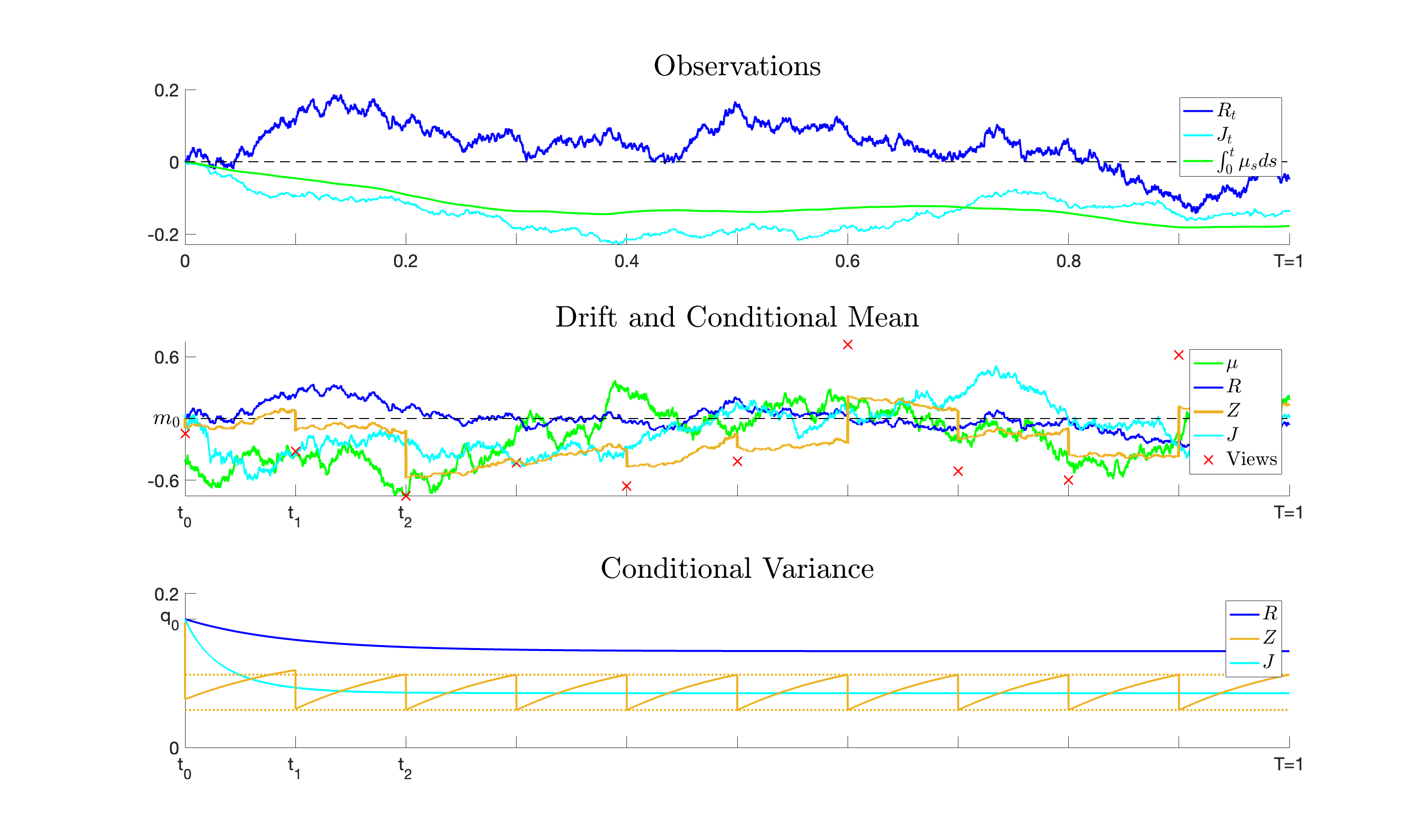
Figure 7.1: Observation and filter processes.   

Top:	Diffusion-type observation processes $\mathbb{R}$ and $J$.
Middle:	Drift $\mu$, expert views $Z_{k}$ and conditional mean $M^{H}$ for $H=R,Z,J$.
Bottom:	Conditional variance $Q^{H}$.

Recall that $Q^{R}$ and $Q^{J}$ as well as $Q^{Z}$ for any $n\in\mathbb{N}$ are deterministic. In the bottom panel one sees that for any fixed $t\in[0,T]$, the value of $Q^{J}_{t}$ as well as the value of $Q^{Z}_{t}$ is less or equal than the value of $Q^{R}_{t}$. This shows that additional information by the expert opinions improves the accuracy of the filter estimate. It confirms the underlying theoretical result on the partial ordering of the conditional covariance matrices as stated in Proposition 3.4. The updates in the filter of the $Z$-investor at the information dates of the expert’s views decrease the conditional variance and lead to a jump of the conditional mean $M^{Z}$. These are typically jumps towards the hidden drift $\mu$, of course this depends on the actual value of the expert’s view. Note that the drift estimate $M^{R}$ of the $R$-investor is quite poor and mostly fluctuates just around the mean-reversion level $\overline{\mu}$. However, the expert opinions visibly improve the drift estimate.

For increasing $t$ the conditional variances $Q_{t}^{R}$ and $Q_{t}^{J}$ approach a finite value. An associated convergence result for $t\to\infty$ has been proven in Proposition 4.6 of Gabih et al. Gabih et al (2014) for markets with $d=1$ stock and generalized in Theorem 4.1 of Sass et al. Sass et al (2017) for markets with an arbitrary number of stocks. For the $Z$-investor we observe an almost periodic behavior of the conditional variance $(Q^{Z}_{t})_{t\geq 0}$. The asymptotic behavior for $t\to\infty$ and the derivation of upper and lower bounds have been studied in detail in Gabih et al. (Gabih et al (2014), , Prop. 4.6) for $d=1$ and in Sass et al. (Sass et al (2017), , Sec. 4.2) for the general case. These bounds are shown as dashed lines in the bottom panel.

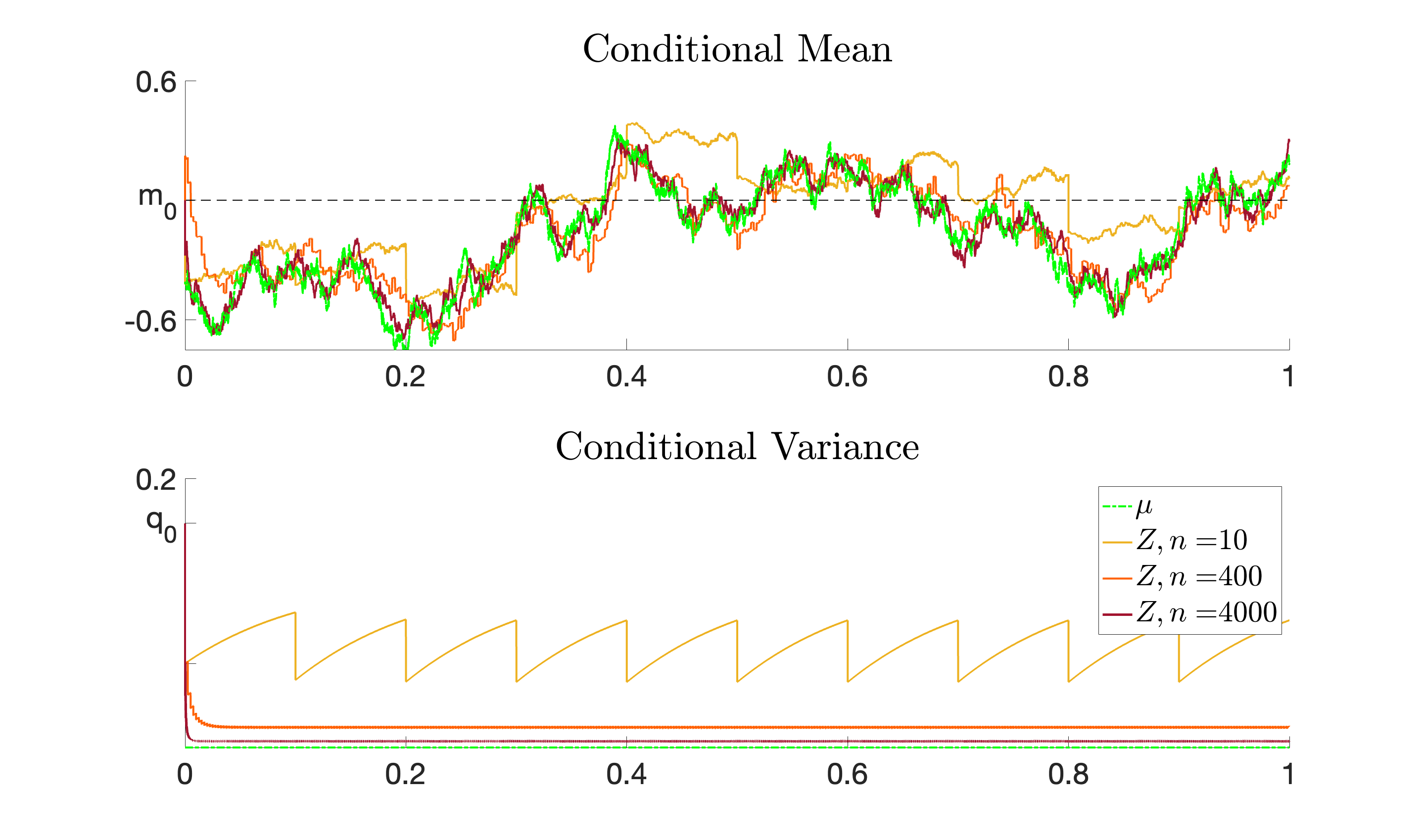
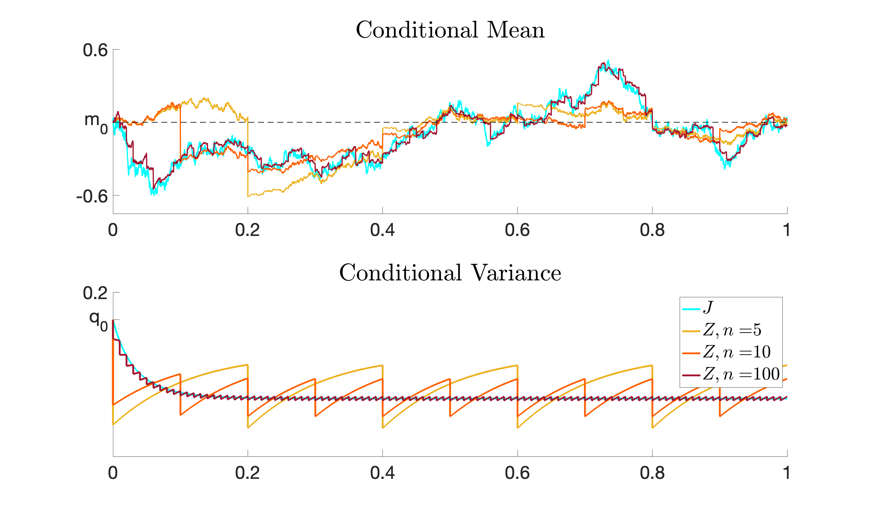
Figure 7.2: Asymptotic behavior of the filter for $n\to\infty$
Left:   Constant expert’s variance $\Gamma=0.1$, convergence to full information
Right: Linearly growing expert’s variance $\Gamma^{(n)}=\frac{n}{T}\sigma_{J}^{2}$, diffusion approximation

Next we perform some experiments illustrating the theoretical results from Subsec. 3.2 on the asymptotic filter behavior for increasing number $n$ of expert opinions. We distinguish two cases. First, the expert’s variance $\Gamma$ stays constant leading to convergence to full information, i.e., mean square convergence of $M^{Z,n}$ to $\mu$ and $Q^{Z,n}\to 0$ on $(0,T]$, see Theorem 3.9. Second, that variance grows linearly with $n$ leading to convergence to the filter processes of the $Z$-invester to those of the $J$-investor, see Theorem 3.11. For that experiment the expert’s views are generated as in (22), i.e., the Gaussian random variables $\varepsilon_{k}$ in (5) are linked with the Brownian motion $W^{J}$ from (6) driving the continuous-time expert opinion process $J$.

Fig. 7.2 shows on the left side for the experiment with constant variance $\Gamma$ the conditional mean $M^{Z,n}$ and the drift $\mu$ (top) and the conditional variance $Q^{Z,n}$ (bottom) for $n=10,400,4000$. It can be nicely seen that for increasing $n$ the conditional variance tends to zero while the conditional mean approaches the drift process for any $t\in(0,T]$. In the limit for $n\to\infty$ the $Z$-investor has full information about the drift process. The panels on the right side show the results for the experiment with linearly growing variance for which we consider the cases $n=5,10,100$. It can be seen that the both filter processes $M^{Z,n}$ and $Q^{Z,n}$ approach the corresponding processes of the $J$-investor for any $t\in[0,T]$ in accordance with Theorem 3.11. Contrary to the first experiment we observe that this convergence is much faster.

Note that for the chosen parameters from Table 1 we have for $n=10$ expert opinions that $\Gamma=\Gamma^{(n)}=\frac{n}{T}\sigma_{J}^{2}=0.1$, i.e., the same expert’s variances for both experiments. This yields for $n=10$ identical conditional variances as it can be seen in the two bottom panels. However, the paths of the conditional mean are different since the expert’s views $Z_{k}$ in the experiment with linearly growing expert’s variance are linked to the Brownian motion $W^{J}$, see (22), whereas in the left panels they are not.

7.3 Value function

In this subsection we present for the case of power utility solutions to the control problem (43). In particular we analyze the value functions $V^{H}(t,m)$ and the associated optimal decision rules $\Pi^{H}(t,m)$ for the different information regimes $H$. They are given in Theorems 4.4, 5.3 and 6.3 for $H=F$, $R,J$ and $Z$, respectively. We recall relation (44) saying that the solution of the original problem of maximizing expected power utility can be obtained from $V^{H}$ by the relation $\pazocal{V}_{0}^{H}(x_{0})=\frac{x_{0}^{\theta}}{\theta}V^{H}(0,m_{0})$. For $H=F$ the relation also holds true if the initial value $m_{0}$ of the conditional mean is replaced by the initial value $\mu_{0}$ of the drift.

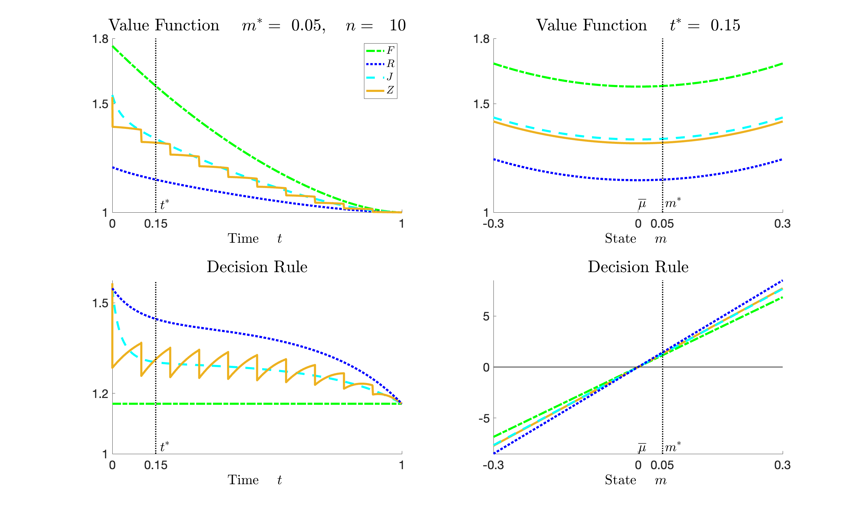
Figure 7.3: Value functions and optimal decision rules.
Top:      Value functions $V^{H}(t,m)$ for $H=F,R,J,Z~{}(n=10)$ depending on $t/m$ (left/right).
Bottom: Optimal decision rule ${\Pi}^{H}(t,m)$ depending on $t/m$ (left/right).

Figure 7.3 shows in the upper part the value functions $V^{H}(t,m)$ for $H=R,Z,J,F$ plotted against time $t$ (left) for a fixed value for the state $m=m^{\ast}=0.05$ and plotted against state $m$ (right) for fixed time $t=t^{\ast}=0.15$. The lower panels show the corresponding decision rules $\Pi^{H}(t,m)$ for the partially informed investors.

For the value functions we can observe that they decay for increasing time $t$ reaching the value $1$ at terminal time $T$ which follows from the definition of the performance criterion in (42). The value function of the $Z$-investor exhibits jumps at the information dates. The upper right panel illustrates that the value functions are exponentials of a quadratic function of the state $m$. For almost all $(t,m)$ the value function of the fully informed investor $V^{F}(t,m)$ dominates those of the partially observed investors. Further, the value functions of the $Z$- and $J$-investor with access to additional information from the expert opinions dominate the value function of $R$-investor observing returns only. We note, that these relations do not hold in general except for $t=0$.

The lower plots show the optimal decision rules $\Pi^{H}(t,m)$ which are given in (45), (60) and (65). They are all of the form, see Remark 5.5 and (55),

$$\Pi^{H}(t,m)=\Pi^{F}(t,m)+\frac{1}{1-\theta}\Sigma_{R}^{-1}Q_{t}^{H}\big{(}2A^{H}(t)m+B^{H}(t)\big{)}~{}~{}\text{with}~{}~{}\Pi^{F}(m)=\frac{1}{1-\theta}\Sigma_{R}^{-1}m.$$

Here, $\Pi^{F}$ constitutes the myopic strategy whereas the correction term $\Pi^{H}-\Pi^{F}$ describes the hedging demand of the partially informed $H$-investor. All decision rules are linear in the state $m$ as it can be seen from the lower right panel. For states $m$ larger (smaller) than the mean reversion level of the drift $\overline{\mu}$ the investors holds a long (short) position in the stock which are smaller (in absolute terms) for the fully informed investor than for partially informed ones. The figures further show that the hedging demand decreases over time (in absolute terms) and vanishes at terminal time $T$. For $H=Z,J$ it is smaller than for $H=R$ indicating that more information about the hidden drift leads to strategies closer to the myopic strategy. This effect is also supported by the observation that the decision rule of the $Z$-investor exhibits jumps at the information dates towards the myopic strategy. The arrival of an additional information improves the filter estimate of the hidden drift and decreases the correction term.

We refer to Kondakji (Kondkaji (2019), , Sec. 8.3) for results for a negative parameter $\theta$, i.e., a relative risk aversion $1-\theta$ larger than for log-utility. Contrary to the present case with $\theta=0.3$ in which the control problem (43) is a maximization problem we face a minimization problem for $\theta<0$. There are similar results but the monotonicity properties w.r.t. time $t$ and the ordering of the value function and optimal decision rules for the different information regimes $H$ are reversed.

7.4 High-Frequency Experts

In this subsection we want to study the asymptotic behavior of the value functions and optimal decision rules of the $Z$-investor for growing number $n$ of expert opinions. For the case of log-utility it is known that the convergence results for the filters as given in Theorems 3.9 and 3.11 carry over directly to the convergence of value functions. The proof is straightforward and relies on representations of the value function as in (24) in terms of an integral functional of the (deterministic) conditional variance $Q^{Z}$.

However, in case of power utility that approach can no longer be adopted since the performance criterion in (42) and consequently the value functions $V^{H}(t,m)$ are now given in terms of expectations of the exponential of quite involved integral functionals of the state processes $L^{H}$. Note that $L^{H}$ is related to the filter process $M^{H}$ of conditional mean under the equivalent measure $\overline{\mathbb{P}}^{H}$ introduced in Subsec. 4.2. Hence, the value functions $V^{H}(t,m)$ depend on the complete filter distribution, not only on its second-order moments. Further, for power utility the optimal strategies do not depend only on the current drift estimate but contain correction terms depending on the distribution of future drift estimates. A formal and rigorous proof of convergence of value functions is ongoing work and deferred to a forthcoming publication. It is based on the $\mathrm{L}^{p}$-convergence of conditional mean processes for arbitrary $p\geq 2$ as it can be deduced from Theorems 3.9 and 3.11.

Our numerical results presented below provide a strong support of the convergence of value functions also for power utility. As in Subsec. 3.2 we consider two different asymptotic regimes which are obtained if the expert’s variance $\Gamma$ is either fixed or grows linear in $n$. In order to emphasize the dependence of the value function and optimal decision rule of the $Z$-investor on $n$ we use the notation ${V}^{Z,n}$ and ${\Pi}^{Z,n}$.

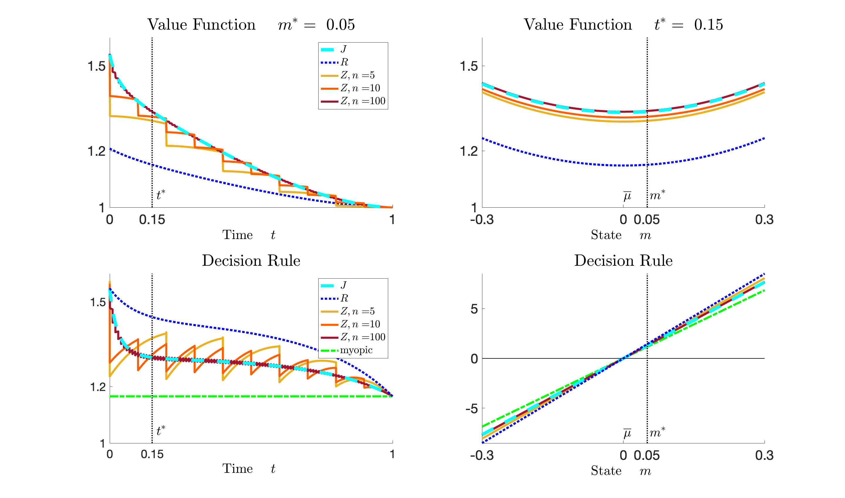
Figure 7.4: Asymptotic behavior of value functions and optimal decisions rules for growing $n$ and $~{}\Gamma^{(n)}=\frac{n}{T}\sigma_{J}^{2}$.
Top:      Value functions $V^{H}(t,m)$ depending on $t/m$ (left/right) for $H=R,J,Z$
Bottom: Optimal decision rules ${\Pi}^{H}(t,m)$ for $H=F,R,J,Z$ depending on $t/m$ (left/right).

Figure 7.4 presents results of experiments for linearly growing variance $\Gamma^{(n)}=\frac{n}{T}\sigma_{J}^{2}$ for which we have convergence of the filter processes $M^{Z,n},Q^{Z,n}$ to the diffusion limit given by filter processes of the $J$-investor observing a continuous-time expert opinion process. The top panels show the value function ${V}^{Z,n}(t,m)$ while the bottom panels present the optimal decision rule ${\Pi}^{Z,n}(t,m)$ of the $Z$-investor observing $n=5,10,100$ expert opinions. For comparison we also show the results for the $R$- and $J$-investor. For increasing $n$ both ${V}^{Z,n}$ and ${\Pi}^{Z,n}$ quickly approach the corresponding quantities of the $J$-investor. This shows that for the chosen parameters quite accurate diffusion approximations of solutions to the control problem for the $Z$-investor are available already for moderate numbers $n$ of expert opinions. Since the latter require less computational effort this is very helpful for deriving approximations not only for the value functions but also for related quantities such as efficiencies and prices of expert opinions introduced in Subsec. 2.6 and considered in the next subsection.

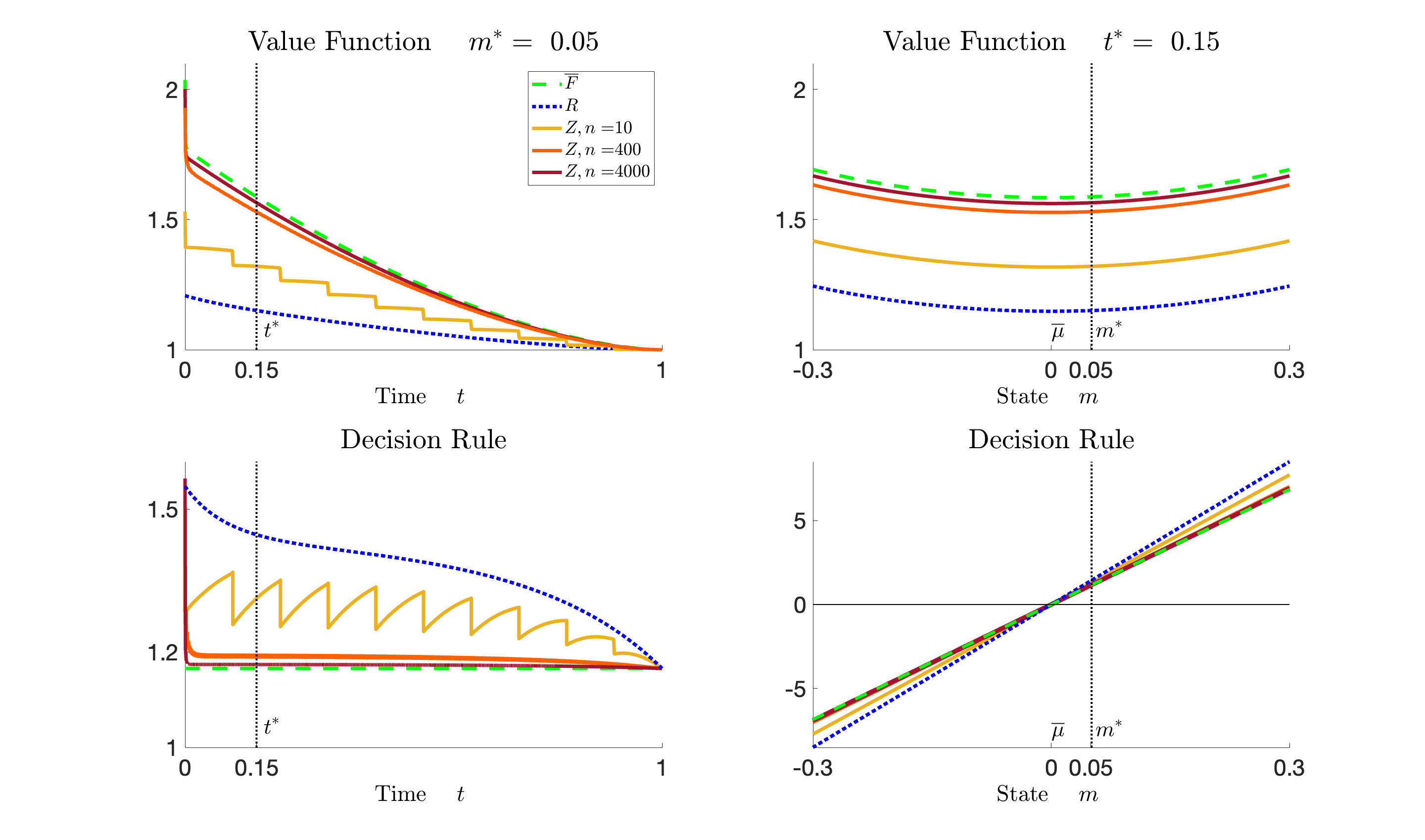
Figure 7.5: Asymptotic behavior of value functions and optimal decision rules for growing $n$ and $~{}\Gamma=0.1$ (fixed).
Top:     Value function $\overline{V}^{F}(t,m,Q_{t}^{{Z},{4000}})$ and ${V}^{H}(t,m)$ depending on $t/m$ (left/right) for $H=R,Z$.
Bottom: Optimal decision rules ${\Pi}^{H}(t,m)$ for $H=F,R,Z$ depending on $t/m$ (left/rights).

Fig. 7.5 shows results of the experiment with fixed variance $\Gamma=0.1$ for which we have convergence to full information, i.e., mean-square convergence of $M^{Z,n}$ to $\mu$ and $Q^{Z,n}\to 0$ on $(0,T]$. As in Fig. 7.4 we plot ${V}^{Z,n}$ and ${\Pi}^{Z,n}$ against time $t$ and state $m$, but now for $n=10,400,4000$. We expect that $|{V}^{Z,n}(t,m)-\overline{V}^{F}(t,m,Q_{t}^{Z,n})|$ converges to zero where $\overline{V}^{F}$ is the conditional expectation of the value function $V^{F}(t,\mu_{t})$ of the fully informed investor given $\pazocal{F}_{t}^{Z,n}$. That function is introduced in (50) and Lemma 51 provides a closed-form expression. The upper panels show for comparison $\overline{V}^{F}(t,m,Q_{t}^{Z,4000})$ and also the value function of the $R$-investor while the bottom panels also show the decision rules of the $R$- and $F$-investor. The latter is independent of time $t$ and defines the myopic strategy. We observe that for increasing $n$ the value function and the optimal decision rule of the $Z$-investor approach $\overline{V}^{F}$ and the myopic decision rule, respectively. However, compared to the case of linearly growing expert’s variance (see Fig. 7.4) the convergence is much slower. This was already observed in Subsec. 7.2 for the convergence of filter processes.

We note again that for the chosen parameters we have for $n=10$ expert opinions that $\Gamma=\Gamma^{(n)}=\frac{n}{T}\sigma_{J}^{2}=0.1$. This yields that for $n=10$ the value function and decision rule for the experiment with linear growing expert’s variance $\Gamma^{(n)}$ coincide with those for the experiment with constant variance $\Gamma$.

7.5 Monetary Value of Information

We conclude this section with some results of experiments illustrating the concepts of efficiency and price of expert opinions introduced in Subsec. 2.6 for the description of the monetary value of information.

Efficency

Recall that we followed an utility indifference approach and considered the initial capital $x_{0}^{H/F}$ which the fully informed $F$-investor needs to obtain the same maximized expected utility at time $T$ as the partially informed $H$-investor who started at time $0$ with wealth $x_{0}^{H}>0$. That wealth is given in Eq. (11) as the solution of the equation $\pazocal V_{0}^{H}(x_{0}^{H})={\mathbb{E}}\big{[}\pazocal V_{0}^{F}\big{(}\text{$x$}_{0}^{H/F}\big{)}\mid\pazocal F_{0}^{H}\big{]}$ for $H=R,Z,J$. The difference $x_{0}^{H}-x_{0}^{H/F}>0$ describes the loss of information for the partially informed $H$-investor relative to the $F-$investor measured in monetary units. The ratio $\varepsilon^{H}={x_{0}^{H/F}}/{x_{0}^{H}}\in(0,1]$ introduced in (12) is a measure for the efficiency of the $H$-investor. We refer to Lemma 5.7 and 6.5 where we give explicit expressions for the above quantities for $H=R,J$ and $H=Z$, respectively.

In Fig. 7.6 we compare the efficiencies of the $Z$-investor for increasing $n$ and parameter of the utility function $\theta=\pm 0.3$. In the left panel the expert’s variance is kept constant and equal to $\Gamma=0.1$. Then the $Z$-investor asymptotically for $n\to\infty$ has full information about the hidden drift. The figure shows that the $Z$-investor’s efficiency increases with $n$ starting with the efficiency of the $R$-investor (blue) and approaching $1$ which is the efficiency of the fully informed investor (green). Note that the investment horizon is $T=1$ year such that arrival of the expert opinions once per year, month, week, day, hour or minute corresponds to $n=1,12,52,365,8.760$ or $525.600$, respectively. Comparing the efficiencies for different parameter $\theta$ it can be seen that an investor with the positive parameter $\theta=0.3$, i.e., more risk averse than the log-utility investor ($\theta=0$), achieves smaller efficiencies than an investor with the negative parameter $\theta=-0.3$. Note that the latter is less risk averse than the log-utility investor. Additional experiments have shown that the efficiency increases with increasing risk aversion $1-\theta$.

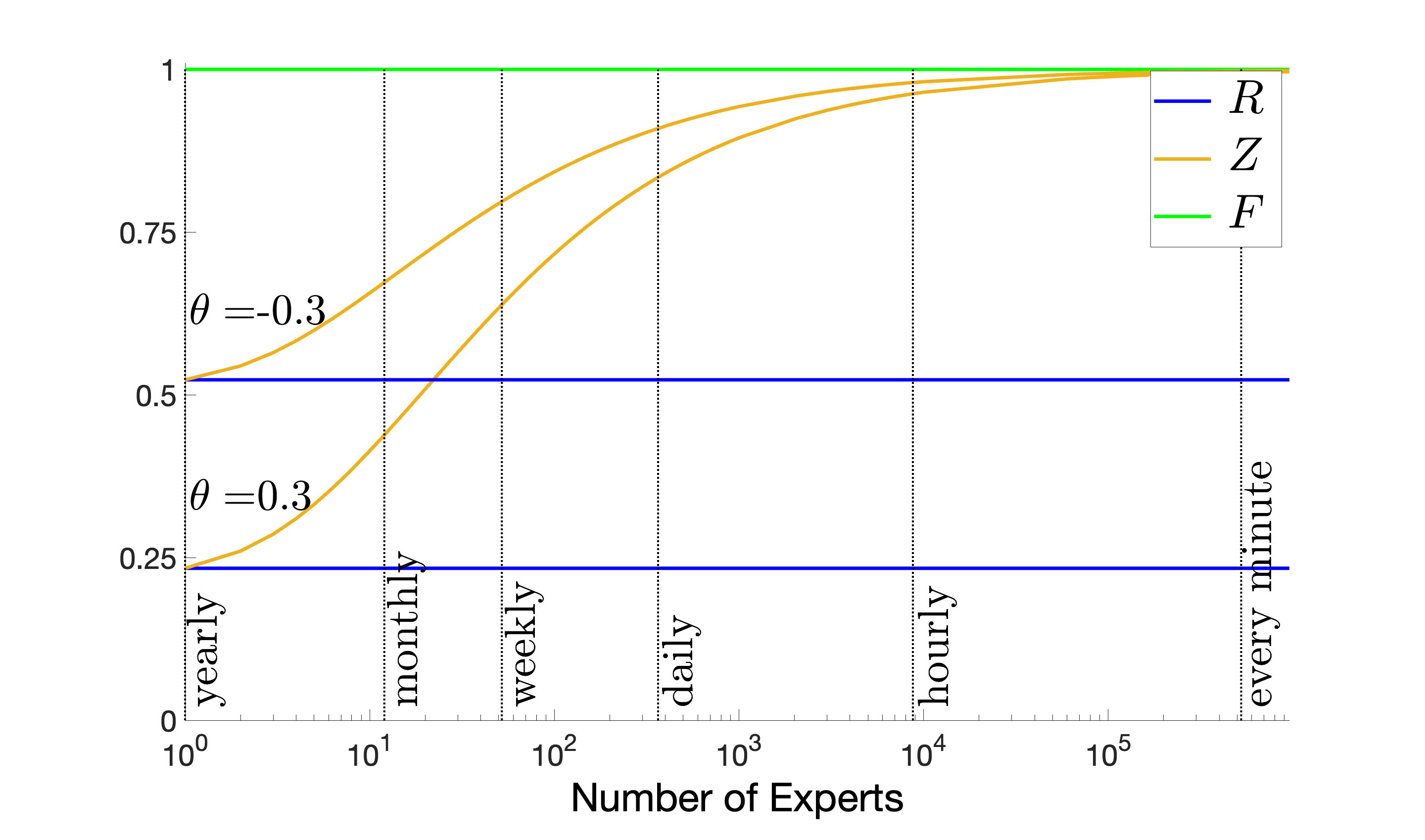
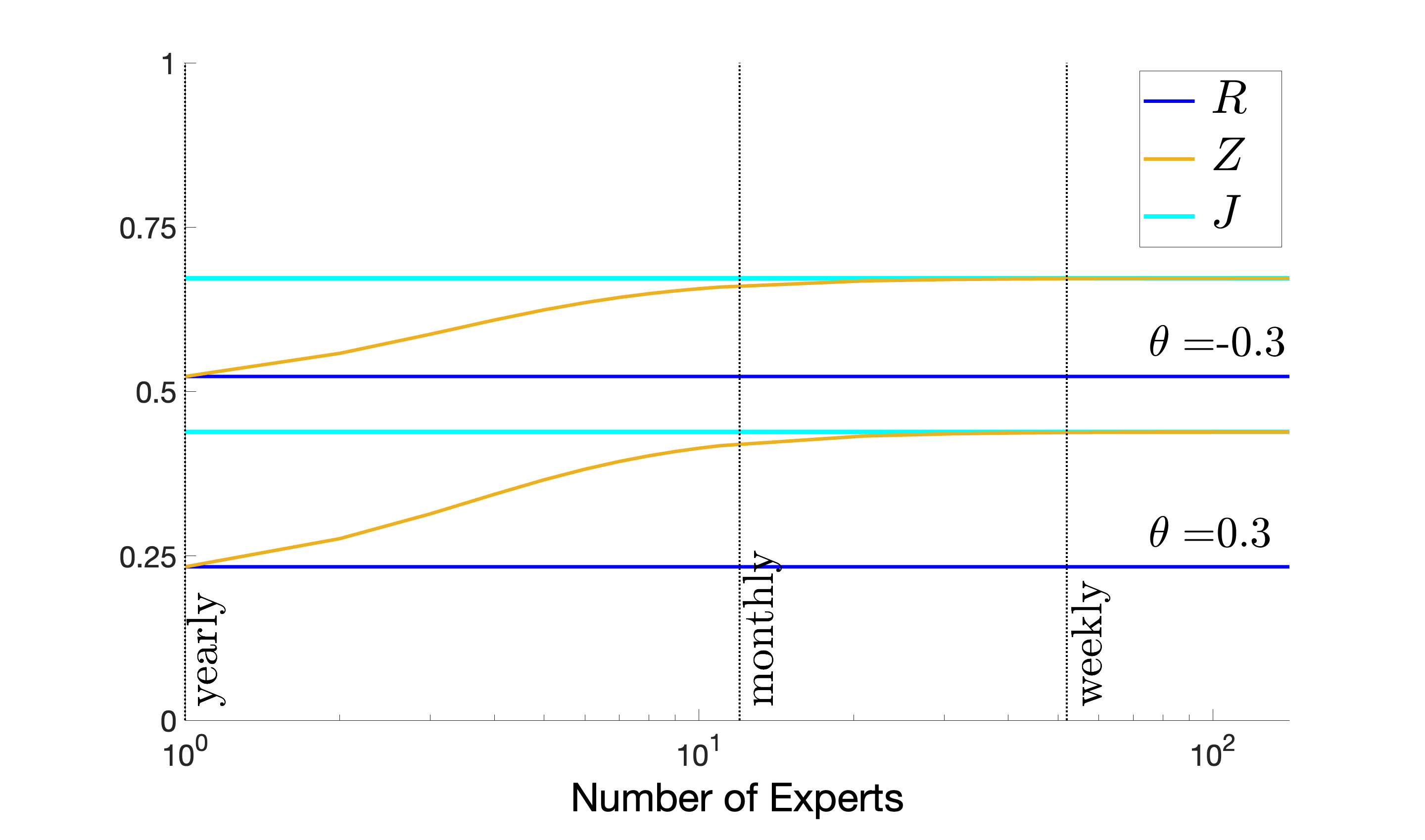
Figure 7.6: Efficiency of the $Z$-investor for increasing $n$ and power utility function with $\theta=\pm 0.3$:
Left:   Expert’s variance $\Gamma=0.1$ fixed;
Right: Expert’s variance $\Gamma^{(n)}=\frac{n}{T}\sigma_{J}^{2}$ linearly growing.

In the right panel in Fig. 7.6 we show results of experiments in which the expert’s variance $\Gamma$ grows linearly with $n$. In that setting we expect convergence to the diffusion limit represented by the $J$-investor. Here, the $Z$-investor’s efficiency again increases with $n$ starting with the efficiency of the $R$-investor (blue) but now approaches the efficiency $\varepsilon^{J}$ of the $J$-investor (light blue) which is less than $1$. As already observed for the value functions in Subsec. 7.4 that convergence is much faster than the convergence to full information for fixed $\Gamma$. The diffusion limit $\varepsilon^{J}$ provides quite accurate approximations for $\varepsilon^{Z,n}$ already for $n\approx 50$, i.e., weekly expert’s views.

Price of the experts

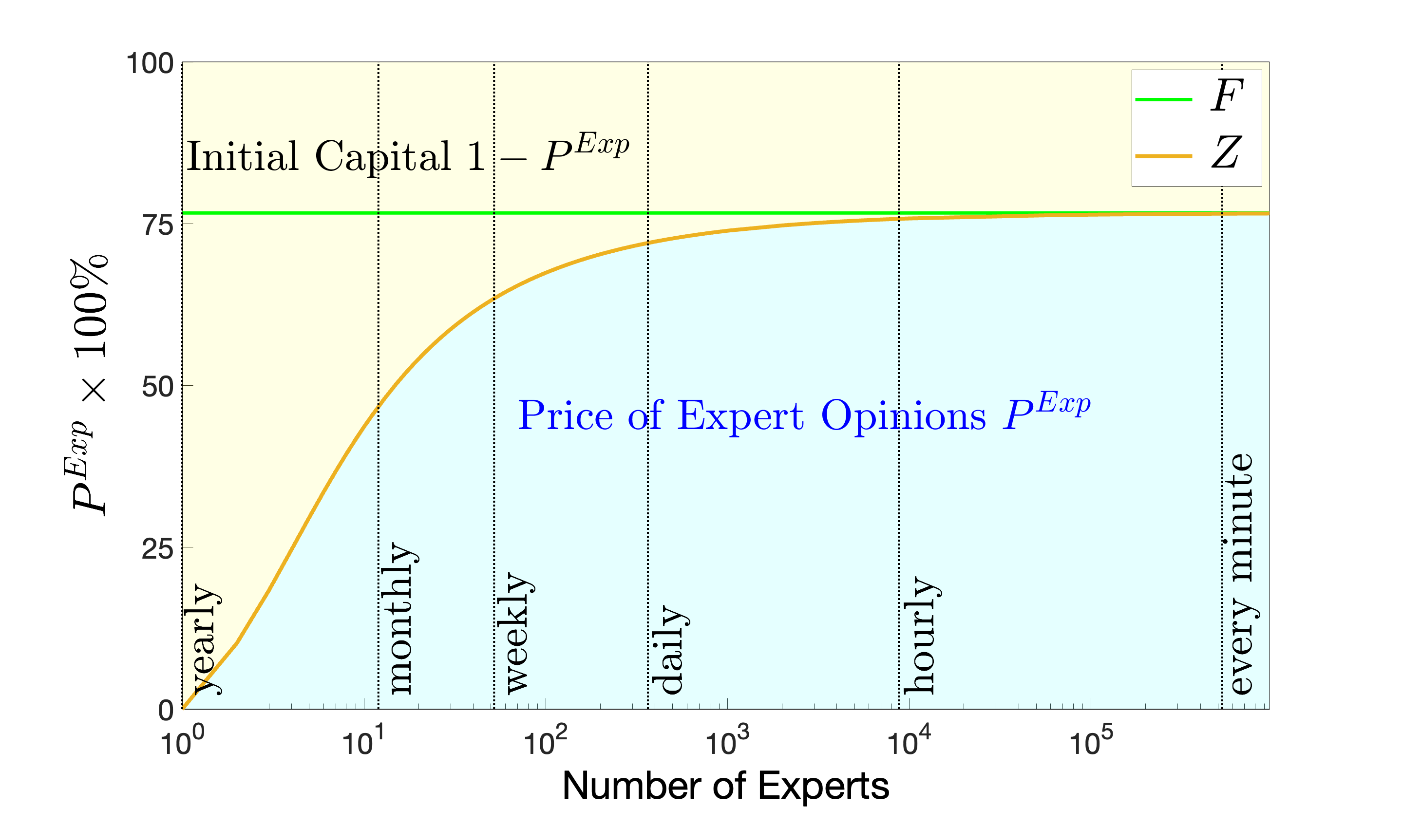
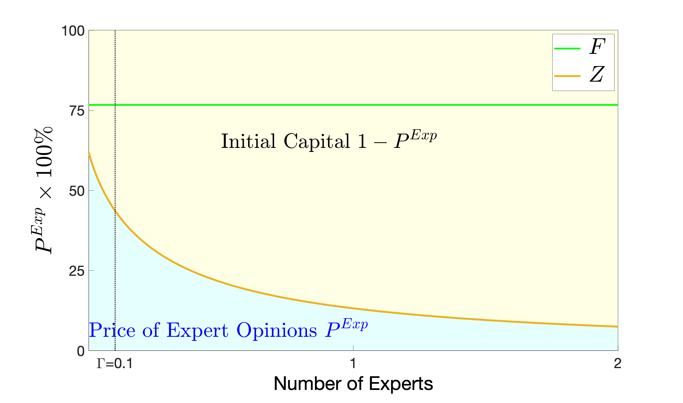
Figure 7.7: Price of the experts for power utility with $\theta=0.3$:
Left:   Increasing number $n$ of expert opinions and expert’s variance $\Gamma=0.1$ fixed;
Right: Increasing expert’s variance $\Gamma$ and $n=10$ fixed.

In Subsec. 2.6 we also used the utility indifference approach to derive a measure for the monetary value of the additional information delivered by the experts. The idea was to equate the maximum expected utilities of an $R$-investor who only observes returns of the $H$-investor for $H=Z,J$. The latter combines return observations with information from the experts. Given the $R$-investor is equipped with initial capital $x_{0}^{R}>0$ one computes the initial capital $x_{0}^{R/H}\leq x_{0}^{R}$ for the $H$-investor which leads to the same maximum expected utility, we refer to Eq. (13). Then the $R$-investor could put aside from its initial capital $x_{0}^{R}$ the amount $P_{Exp}^{H}:=x_{0}^{R}-x_{0}^{R/H}\geq 0$ to buy the information from the expert. The remaining capital $x_{0}^{R/H}$ is invested in an $H-$optimal portfolio and providing the same expected utility of terminal wealth as the $R$-optimal portfolio starting with initial capital $x_{0}^{R}$. We refer to Lemma 5.7 and 6.5 where we give explicit expressions for $P_{Exp}^{H}$ for $H=J$ and $H=Z$, respectively.

Fig. 7.7 shows the above decomposition of the initial capital of the $R$-investor for $x_{0}^{R}=1$. In the left panel we fix the expert’s variance $\Gamma=0.1$ and plot $P_{Exp}^{Z,n}$ against $n$. As expected that price increases with the number of expert opinions but for $n\to\infty$, i.e., in the full information limit, the price reaches a saturation level which is given by $x_{0}^{R}-x_{0}^{R/F}=1-\varepsilon^{R}$.

The right panel shows results for fixed $n=10$ but growing variance $\Gamma$. Then the expert’s views provide less and less information about the hidden drift leading to a decreasing price $P_{Exp}^{Z}$ approaching zero for $\Gamma\to\infty$, i.e., for fully non-informative expert’s views. On the other hand in the limiting case for $\Gamma\to 0$ at each of the $n=10$ information dates the $Z$-investor has full information about the drift process. Note that full information is not available for all for all $t\in(0,T]$ but only at finitely many information dates and thus $P_{Exp}^{Z}$ is for $\Gamma\to 0$ moving towards but not reaching the full information limit $1-\varepsilon^{R}$.

Acknowledgments The authors thank Dorothee Westphal and Jörn Sass (TU Kaiserslautern) and Benjamin Auer (BTU Cottbus-Senftenberg) for valuable discussions that improved this paper

Conflict of interest The authors have no competing interests to declare that are relevant to the content of this article. No funding was received to assist with the preparation of this manuscript.

References

- (1) Angoshtari, B.: Stochastic Modeling and Methods for Portfolio Managment in Cointegrated Markets. PhD thesis, University of Oxford, https://ora.ox.ac.uk/objects/uuid:1ae9236c-4bf0-4d9b-a694-f08e1b8713c0 (2014).
- (2) Benth, F. E., and Karlsen, K. H.: A note on Merton’s portfolio selection problem for the Schwartz mean-reversion model, Stochastic Analysis and Applications 23(4), 687–704 (2005).
- (3) Bielecki, T.R, and Pliska, S.R: Risk-sensitive dynamic asset management. Applied Mathematics and Optimization 39 , 337–360 (1999).
- (4) Björk, T., Davis, M. H. A. and Landén, C.: Optimal investment with partial information, Mathematical Methods of Operations Research 71 , 371–399 (2010).
- (5) Black, F. and Litterman, R.: Global portfolio optimization. Financial Analysts Journal 48(5), 28-43 (1992).
- (6) Brendle, S.: Portfolio selection under incomplete information. Stochastic Processes and their Applications, 116(5), 701-723 (2006).
- (7) Brennan, M.J., Schwartz, E.S., Lagnado, R.: Strategic asset allocation. Journal of Economic Dynamics and Control 21 (8), 1377–1403 (1997).
- (8) Broadie, M.: Computing efficient frontiers using estimated parameters. Annals of Operations Research 45, 21–58 (1993).
- (9) Chen, K. and Wong, Y.: Duality in optimal consumption–investment problems with alternative data. arXiv:2210.08422 [q-fin.MF] (2022).
- (10) Colaneri, K., Herzel, S. and Nicolosi, M.: The Value of knowing the market price of risk. Annals of Operations Research 299, 101–131 (2021).
- (11) Davis, M. and Lleo, S.: Black-Litterman in continous time: the case for filtering. Quantitative Finance Letters, 1,30-35 (2013).
- (12) Davis, M. and Lleo, S.: Debiased expert opinions in continuous-time asset allocation. Journal of Banking & Finance, Vol. 113, 105759 (2020).
- (13) Davis, M. and Lleo, S.: Jump-diffusion risk-sensitive benchmarked asset management with traditional and alternative data. Annals of Operations Research (2022). DOI:10.1007/s10479-022-05130-3
- (14) Elliott, R.J., Aggoun, L. and Moore, J.B.: Hidden Markov Models, Springer, New York, (1994).
- (15) Fouque, J. P, Papanicolaou, A. and Sircar, R.: Filtering and portfolio optimization with stochastic unobserved drift in asset returns. SSRN Electronic Journal,13(4):935-953, (2015).
- (16) Frey, R., Gabih, A. and Wunderlich, R.: Portfolio optimization under partial information with expert opinions. International Journal of Theoretical and Applied Finance, 15, No. 1, (2012).
- (17) Frey, R., Gabih, A. and Wunderlich, R.: Portfolio optimization under partial information with expert opinions: Dynamic programming approach. Communications on Stochastic Analysis Vol. 8, No. 1, 49-71 (2014).
- (18) Gabih, A., Kondakji, H. Sass, J. and Wunderlich, R.: Expert opinions and logarithmic utility maximization in a market with Gaussian drift. Communications on Stochastic Analysis Vol. 8, No. 1,27-47 (2014).
- (19) Gabih, A., Kondakji, H. and Wunderlich, R.: Asymptotic filter behavior for high-frequency expert opinions in a market with Gaussian drift. Stochastic Models 36(4), 519-547 (2020).
- (20) Gabih, A., Kondakji, H. and Wunderlich, R.: Well posedness of utility maximization problems under partial information in a market with Gaussian drift. submitted, arXiv:2205.08614 [q-fin.PM] (2022).
- (21) Kim, T. S. and Omberg, E.: Dynamic non myopic portfolio behavior, The Review of Financial Studies 9(1), 141-16 (1996).
- (22) Kondakji, H.: Optimal Portfolios for Partially Informed Investors in a Financial Market with Gaussian Drift and Expert Opinions (in German). PhD Thesis BTU Cottbus-Senftenberg. Available at https://opus4.kobv.de/opus4-btu/frontdoor/deliver/index/docId/4736/file/Kondakji_Hakam.pdf, (2019).
- (23) Lakner, P.: Optimal trading strategy for an investor: the case of partial information. Stochastic Processes and their Applications 76, 77-97 (1998).
- (24) Liptser, R.S. and Shiryaev A.N.: Statistics of Random Processes: General Theory, 2nd edn, Springer, New York, (2001).
- (25) Merton, R.: Optimal consumption and portfolio rules in a continuous time model. Journal of Economic Theory 3, 373-413 (1971).
- (26) Nagai, H. and Peng, S.: Risk-sensitive dynamic portfolio optimization with partial information on infinite time horizon. The Annals of Applied Probability 12, 173-195 (2002).
- (27) Pham, H.: Optimal stopping of controlled jump diffusion processes: A viscosity solution approach. Journal of Mathematical Systems, estimations, and Control Vol.8, No.1, 1-27 (1998).
- (28) Putschögl, W. and Sass, J.: Optimal consumption and investment under partial information, Decisions in Economics and Finance (31), 131–170 (2008).
- (29) Rieder, U. and Bäuerle, N.: Portfolio optimization with unobservable Markov-modulated drift process. Journal of Applied Probability 43, 362-378 (2005).
- (30) Rogers, L.C.G.: Optimal Investment. Briefs in Quantitative Finance. Springer, Berlin-Heidelberg, (2013).
- (31) Sass, J. and Haussmann, U.G.: Optimizing the terminal wealth under partial information: The drift process as a continuous time Markov chain. Finance and Stochastics (8), 553-577 (2004).
- (32) Sass, J., Westphal, D. and Wunderlich, R.: Expert opinions and logarithmic utility maximization for multivariate stock returns with Gaussian drift. International Journal of Theoretical and Applied Finance Vol. 20, No. 4, 1-41 (2017).
- (33) Sass, J., Westphal, D. and Wunderlich, R.: Diffusion approximations for randomly arriving expert opinions in a financial market with Gaussian drift. Journal of Applied Probability, 58(1), 197 - 216 (2021).
- (34) Sass, J., Westphal, D. and Wunderlich, R.: Diffusion approximations for periodically arriving expert opinions in a financial market with Gaussian drift. Stochastic Models (2022), DOI:10.1080/15326349.2022.2100423
- (35) Schöttle, K., Werner, R. and Zagst, R.: Comparison and robustification of Bayes and Black-Litterman models. Mathematical Methods of Operations Research 71, 453–475 (2010).
- (36) Xia, Y.: Learning about Predictability: The Effects of parameter uncertainty on dynamic asset allocation. Journal of Finance, Vol. 56, No. 1, 205-246.